Embed Size (px)
Citation preview
INTERNATIONAL JOURNAL OF RESEARCH AND INNOVATION
™©all copyrights reserved [email protected] | [email protected]
572
Subject: Thermal Engineering IJRITE
ANALYSIS OF CONJUGATE HEAT TRANSFER IN MICRO FIBERS
B. Srikanth1, Medapati Sreenivasa Reddy2.
1 Research Scholar, Department of Mechanical Engineering, Aditya Engineering College, Surampalem, Andhra Pradesh, India.
2 Professor, Department of Mechanical Engineering, Aditya Engineering College, Surampalem, Andhra Pradesh, India.
Abstract
The present work on ANALYSIS OF CONJUGATE HEAT TRANSFER IN MICROFIBERS an extensive study is conducted
for convective flow in a microfiber subjected to partial heating situation. The effect AXIAL BACK HEAT is explained in
a microfiber, which is developed when a developing laminar flow and heat exchange are simultaneously seen on a heat
transfer surface. The present thesis takes in to consideration that the outer surface is maintained at a unvarying wall
temperature and other boundary conditions are: (i) The total span of the microfiber will be subjected to unvarying
temperature. (ii) Ten percentage of span of inlet and outlet of the microfiber are insulated and remaining span will be
subjected to unvarying temperature. (iii) Ten percentage of span of inlet of the microfiber is insulated remaining span
will be subjected to unvarying temperature. (iv) Ten percentage of span of outlet of the microfiber is insulated
remaining span will be subjected to unvarying temperature. An investigation on Computational fluid dynamic analysis
is conducted for the above mentioned situations at wide range of conductivity ratios, Reynolds numbers, and
thickness to diameter ratios. The result variations and inferences are discussed in detail.
*Corresponding Author:
B. Srikanth, Research Scholar,
Department of Mechanical Engineering,
Aditya Engineering College, Surampalem, Andhra Pradesh, India.
Email: [email protected].
Year of publication: 2017
Paper Type: Review paper
Review Type: peer reviewed
Volume: IV, Issue: I
*Citation: B. Srikanth, Research Scholar “Analysis of
Conjugate Heat Transfer In Micro Fibers” International
Journal of Research and Innovation (IJRI) 4.1 (2017) 572-580.
Introduction
About Axial Back Conduction:
Let us consider the two situation one is constant heat
flux and another is constant wall temperature. For the
first situation microfiber is subjected to constant heat
flux on its outer surface. Whenever the heat applied on
the outer surface, flows along the solid wall of the
microfiber by means of conduction. it reaches the
fluid–solid interface, the heat flows in to the water and
get carried along with the fluid flow. The heat is added
continuously to the fluid in the direction of the flow.
The bulk fluid temperature is increasing linearly
because of surface area is increasing linearly in the
direction of flow. So, the wall temperature of microfiber
is also increase linearly in the direction of fluid flow.
We can find the wall temperature of microfiber is given
by:

INTERNATIONAL JOURNAL OF RESEARCH AND INNOVATION
™©all copyrights reserved [email protected] | [email protected]
573
We can find the wall temperature of microfiber by
using the above equation.
(
)
Graph between local wall, bulk fluid temperature and
length of the microfiber (a) constant wall heat flux (b)
constant wall temperature.
Figure.1.1 (a) we can observe that graph between local
wall, bulk fluid temperature and length of the
microfiber at constant wall heat flux. In the second
situation the microfiber is subjected to constant wall
temperature on its outer surface, the local wall, bulk
fluid temperature is nonlinear. We can observe the
graph between local wall, bulk fluid temperature and
length of the microfiber at constant wall temperature
on its outer surface of microfiber form figure 1.1 (b).
The bulk fluid temperature approaches equal to
surface temperature at the outlet of the microfiber. By
the consider these two situation, let us take any two
points on axial direction (both solid and liquid) there is
a maximum temperature between outlet and inlet of
the This axial high temperature distinction leads to
potential for thermal conduction axially along the
strong, furthermore along the fluid towards bay of the
fibre i.e. in a bearing inverse to the heading of fluid
stream. Such a circumstance is known as "axial back
conduction" and prompts conjugate temperature
exchange. Starting currently it is normal that beneath
such ailment there won't be any heat conduction, yet
needs to affirm this from the present work.
LITERATURE REVIEW
The concept of axial back conduction is not another
idea, somewhat an entrenched idea at this point.
Furthermore this idea is not constrained to micro
channels as it were. A point by point audit on early
advancements on axial wall conduction in customary
size heat exchangers is exhibited by Peterson (1999).
Numerous studies do exist in open writing that
arrangement with axial wall conduction in customary
size channels.
For a 3D rectangular moulded micro channel
numerical reproduction was completed by Moharana
and et al, (2012). In this investigation a substrate of
altered size (0.5 mm x 0.4 mm x 50 mm) was chosen
and the channel tallness and width were shifted
autonomously such that the micro channel angle
proportion shifts from 1.0 to 4.0. And Moharana et al,
(2012) found the impact of micro channel angle
proportion on axial back conduction. The Continuous
heat flux limit condition was connected at the base of
the substrate while all its different surfaces have been
kept protected. After the reproduction it was found
that the normal Nu was least relating to channel
perspective proportion of 3.0, regardless of the
conductivity proportion of the working fluid and the
solid substrate
Rahimi and et al. (2012) concentrated on the axial heat
conduction impact on the local Nu. at the passage and
completion district of roundabout small scale funnel.
He suggested the outcome for steady heat flux limit
condition
Moharana et al. (2012) contemplated the impact of
axial conduction in a microfiber for extensive variety of
Re, proportion of wall thickness to internal width and
thermal conductivity proportion. A two dimensional
numerical recreation has been completed for both,
consistent wall heat flux and steady wall temperature,
at the external surface of the fibre, while stream of
fluid through the microfiber is laminar, all the while
creating in nature. After the re-enactment it has been
demonstrated that ksf assumes an overwhelming part
in the conjugate heat exchange process. At the point
when the steady heat flux limit condition is connected
on the external surface of the microfiber, there exists
an ideal estimation of ksf for which the normal Nusselt
number (Nuavg.)
SIMULATION
This is the two dimensional analysis is carried by
Ansys Fluent to understand the effect of axial back
heat of microfiber will be exposed to the unvarying
temperature for four different situations. These
situations are discussed below.

INTERNATIONAL JOURNAL OF RESEARCH AND INNOVATION
™©all copyrights reserved [email protected] | [email protected]
574
Situation 1: The total span of the microfiber will be
subjected to unvarying temperature. see
Fig.
Situation 2: Ten percentage of span of inlet and outlet
of the microfiber are insulated and
remaining span will be subjected to
unvarying temperature; see Fig.
(a) Total span of the microfiber is heating.
(b) Ten percentage of span of inlet and outlet of the microfiber are insulated
Assumptions:
The fluid flow inside in the microfiber is done on
the following assumptions.
1. Steady-state condition.
2. Laminar flow.
3. Incompressible flow.
4. Single phase.
5. Constant thermos physical properties.
3.2 Dimensions of the Microfiber:
Inner radius of microfiber δf
= 0.2 mm
Length of the microfiber L =60 mm
The ratio of thickness to internal radius of microfiber δsf =1 to 10
The ratio of thermal conductivity of solid to fluid Ksf =2.26 to 646.21
3.3 2d Modelling:
We have done modelling and solved the above
problem using Ansys-Fluent. We have drawn the two
dimensional diagram for microfiber using ansys 16
version. The below figure is 2d model of microfiber of
δsf =10.
2d modelling of microfiber
3.3 Grid independence test:
After the modelling the grid independence test is very
important for simulation. In this area we have
considered three different grid sizes of 3600*30,
4200*35 and, 4800*40. The below graph 3.3.(a) shows
between Nu number for zero wall thickness of
microfiber is heated at outer surface constantly. This
figure incorporates both creating and completely
created zone for three diverse cross section sizes of
3600x30, 4200x35 and 4800x40 (for half of the
transverse area), for Re = 100. The local Nu number at
the completely created stream administration (close to
the fibre outlet) changed by 0.8% from the cross
section size of 3600x30 to 4200x35, and changed by
under 0.4% on further refinement to work size of
4800x40. Changing from first to the third work, no

INTERNATIONAL JOURNAL OF RESEARCH AND INNOVATION
™©all copyrights reserved [email protected] | [email protected]
575
obvious change is watched. In this way, the last
framework (4800x40) was chosen.
(a) Meshing of microfiber (size of 3600x30)
(b) Meshing of microfiber (size of 4200x35)
(c) Meshing of microfiber (size of 4800x40)
Boundary Conditions:
Boundary conditions of microfiber for different
situation are:
At, Z=0 to Z =L and r =0, symmetric axis
(3.5)
At, Z=0 and r=0 to r =δf, u =ū
(3.6)
At, Z=L and r=0 to r =δf gauge pressure
(3.7)
At, z=0 & r =δf to r=δs +δf,∂T/∂z = 0
(3.8)
At, z=L & r=δf to r=δs +δf,∂T/∂z = 0
(3.9)
z=0 to L, r=δs +δf,
(3.10)
Ansys fluent trademark is helpful in comprehending be
needed differential equations. For weight data
distribution, standard plan was made use of. The
calculation of speed weight coupling in the multi
Framework arrangement system was given using
SIMPLE calculation. Second arrange upwind when was
the reason behind the comprehension of momentum
and energy equations.The value of 10 -6 is utilised as a
datum for coherence and energy questions while for
vitality equations data is in the order of 10 -9. Water
enters the microfiber with a slug speed profile.
RESULTS AND DISCUSSION
As earlier discussed in simulation, the microfiber inner
radius is constant. The wall thickness of the microfiber
will be varied from 1 to 10, to know the impact of wall
thickness on the behaviour of the heat transfer. Let us
consider a laminar flow of fluid through a microfiber
subjected to either steady wall high temperature or
steady heat flux, we can find the highest transfer
coefficient, when the solid fluid interface experienced
by steady heat flux. Under perfect situations (where
wall thickness is equal to zero), we can find the value
of the Nusselt number will be 4.36,if solid fluid
interface experienced by steady heat flux. And nusselts
number will be 3.66 for steady wall temperature. For
all intents and purposes each waterway will devour
some limited barricade thickness and in light of
conjugate high temperature exchange conditions not
ensured to take the same limit situation at the solid-
fluid boundary which connected on the external
surface of the fibre. The target of this work is to locate
the genuine limit condition experienced at the rock-
hard-fluid crossing point of a microfiber endangered to

INTERNATIONAL JOURNAL OF RESEARCH AND INNOVATION
™©all copyrights reserved [email protected] | [email protected]
576
fractional heating by consistent barricade temperature
at external surface.
Constraints at concentration were axial variety of wall high temperature, greater part liquefied temperature, and home-grown(Nu) . In the 1st place, "Case-1" the total length of the microfiber is heated . Fig. 1.1. Shows the variation of wall temperature and fluid temperature under perfect situation. Figure 4.1 demonstrates dimensionless wall and best part fluid temperature as a component of δsf and Re. The wiped contour speaks to straight variety of main part fluid temperature between the bay and the outlet of the micro duct; its restricting qualities in dimensionless structure are 0 and 1. Under perfect conditions, the bulk fluid high temperature changes directly among the bay and the exit if the fibre is imperilled to steady heat flux limit condition. At lower stream Reynolds number 100 and less estimation for δsf (=1), axial variety of major fluid temperature can be seen to be far from straight variety and near the illustrative variety which is the situation when the fibre is subjected to
consistent wall temperature situation. The outcomes in above graph are autonomous of ksf with the exception of at low estimation of ksf = 2.26. Besides, the wall temperature is verging on steady all through the length of the fibre aside from close to the channel; because of creating stream. An examination of prompts the supposition that the concrete watery boundary for this case encountering consistent wall malaise;which is precisely equivalent to the genuine limit state connected at external surface of the fibre. This implies for this case there is not at all axial stream at heat to mutilate limit complaint at rock-hard-liquid crossing point.
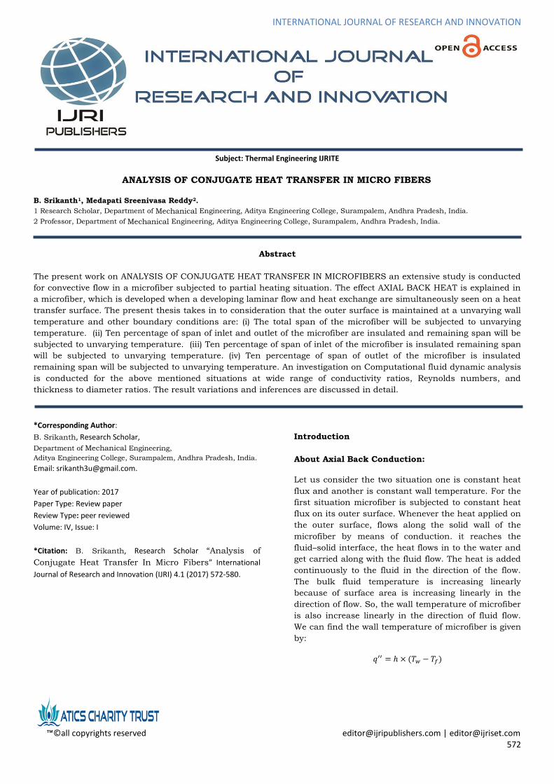
Graph between wall, fluid temperature and length of
microfiber for situation-1
Next, the estimation of δsf expanded from 1 to 10, while
every single other parameter continuing as before as in
graph (a). Presently, it seen in 4.1(b) that the outcomes
not any high autonomous of ksf. Furthermore, the
mainstream fluid temperatures are similarly nearer to
specked contour, showing that the genuine limit
condition next to the solid-fluid crossing point is
floating missing from the isothermalization. Which
likewise be affirmed at the estimations of fence
temperatures; which were not any more consistent for
low estimations of ksf. This demonstrates lower
conductive wall material and upper wall thickness
floats as of real limit condition first.
Temperature variation of microfiber with variation of
δsf =1 and 10 for situation 1
In Case-2, the length of inlet and outlet of 6mm of the microfiber is protected. Actually the fluid temperature
and wall temperature of the microfiber must be equal to the initial temperature of the fluid.. The two vertical specked lines speak to the heating measurement of the microfiber. As a result of inadequate conductivity of the hedge material, there will be conduction of heat in the wall close to the gulf in a course inverse to the bearing of stream of fluid. This will be seen where bulk liquid temperature begins transcending zero in the middle of z = 0 to 6 mm (i.e. z* = 0 to 0.0215). For most minimal ksf the estimation of bulk fluid temperature and in addition wall high temperature are verging on equivalent to zero and consistent in the extent z = 0 to 6 mm (i.e. z* = 0 to 0.0215). With expanding ksf, the estimation of both the wall and the bulk temperature begins ascending in the protected region close to the bay. Because of axial back conduction in the wall of the microfiber. Greater the estimation about f, less the obduracy to stream of heat by conduction; consequently more the ascent in both
the wall and the bulk fluid temperature.
Graphs above relates to δsf = 1 while graph 4.2 (b) relates to δsf = 10. Higher region of fractious-area of solid prompts low updraft imperviousness to axial conduction under same conditions. This can be seen by direct examination amongst the incline of wall temperature in the locale z < 6 mm (or z* < 0.0215) is higher contrasted with its partner in Fig.
INTERNATIONAL JOURNAL OF RESEARCH AND INNOVATION
™©all copyrights reserved [email protected] | [email protected]
577
Graph between wall, fluid temperature and length of microfiber for situation-2.
Next, for higher stream Re, the bulk fluid temperature
floats from illustrative towards straight variety in the
middle of the two dabbed vertical lines, which
compares to the heated zone. This demonstrates
higher stream Re prompts the condition at the solid-
fluid interface more towards dependable wall heat
mutability than secure wall temperature
Microfiber protected on external surface in locale z > 54 mm . In this area the majority fluid temperature rests practically steady the instance of δsf = 1. This because on account of as there is not any heat expansion in this locale. Besides, the partition temperature is marginally greater than the majority of fluid temperature, along these lines there is not at all any heat exchange from the wall to fluid with the exception of at the least ksf. For (ksf = 2.26) , the contrast amongst the fluid and wall temperature is most extreme contrasted with other ksf values toward the begin of end protection. In this way for ksf = 2.26,
the wall temperature begins to diminish at last protected locale toward stream of liquid. For greater stream the Re, the distinction amongst bulk liquefied and the fortification temperature is high at z = 54 mm and z* = 0.194 contrasted with less stream Regarding (contrast at graph. 4.2(e) and Fig. 4.2(a)). Consequently this situation temperature begins diminishing toward stream of liquid because of exchange of heat across the wall to the fluid.
Temperature variation of microfiber with variation of
δsf =1 and 10 for situation 2
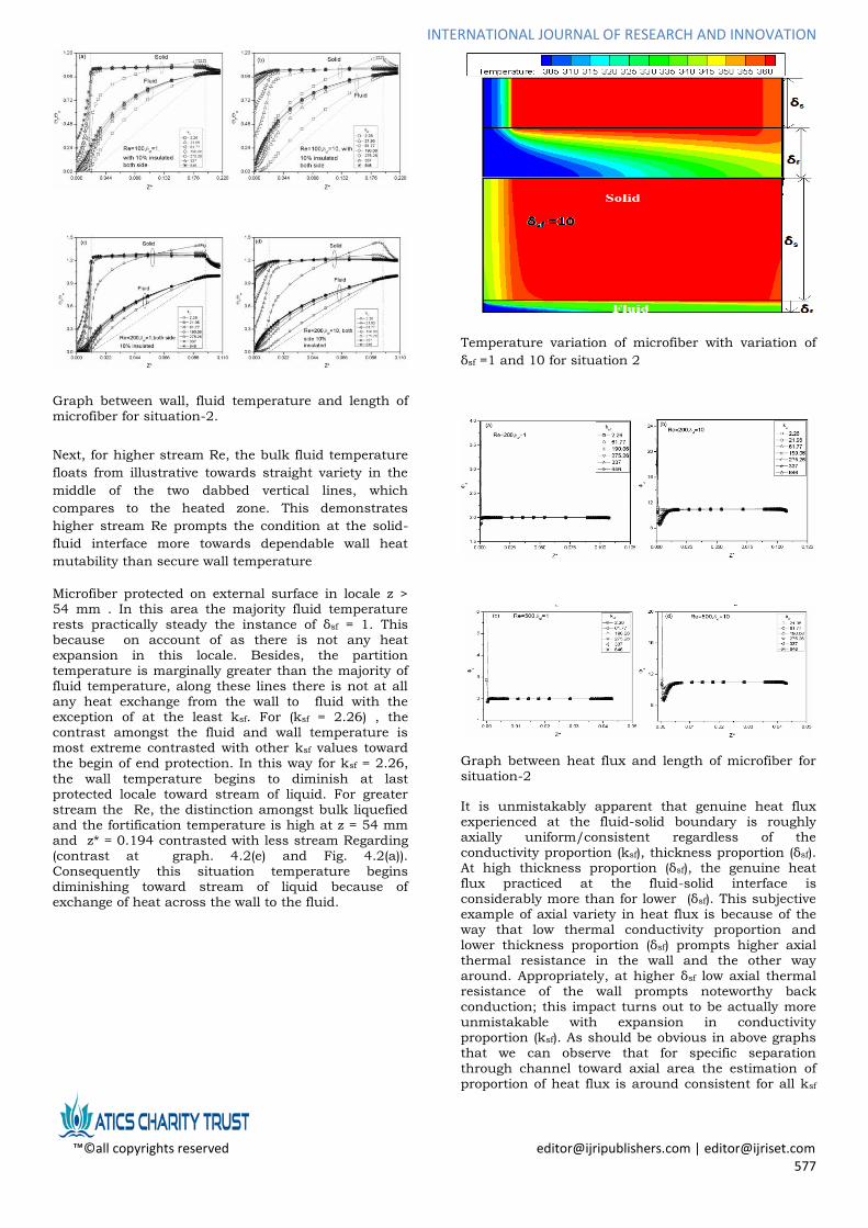
Graph between heat flux and length of microfiber for situation-2
It is unmistakably apparent that genuine heat flux experienced at the fluid-solid boundary is roughly axially uniform/consistent regardless of the conductivity proportion (ksf), thickness proportion (δsf). At high thickness proportion (δsf), the genuine heat flux practiced at the fluid-solid interface is considerably more than for lower (δsf). This subjective example of axial variety in heat flux is because of the way that low thermal conductivity proportion and
lower thickness proportion (δsf) prompts higher axial thermal resistance in the wall and the other way around. Appropriately, at higher δsf low axial thermal resistance of the wall prompts noteworthy back conduction; this impact turns out to be actually more unmistakable with expansion in conductivity proportion (ksf). As should be obvious in above graphs that we can observe that for specific separation through channel toward axial area the estimation of proportion of heat flux is around consistent for all ksf

INTERNATIONAL JOURNAL OF RESEARCH AND INNOVATION
™©all copyrights reserved [email protected] | [email protected]
578
with worth about equivalent to 2 and 10 for the instance of δsf = 1
and 10 separately. And additionally this outcome is
likewise similar at high Re as appeared in Fig. 4.5(c)
and Fig. 4.5(d). Heat flux at solid-fluid interface is
mostly rely on upon wall thickness when external
fringe steady wall temperature is connected which can
be observed by these plots.
Graph between heat flux and length of microfiber for
situation-2
From fig. 4.5-4.6 it is clear that for all condition as
illustrated earlier as four cases and shown
inFig.3.2,theheatflux( )is strong function of δsf. But
it is a week function of Re and ksf due to axial back
condition
Immediate ramifications the axial variety of bulk fluid
temperature and dimensionless wall, and
dimensionless wall heat chooses estimation native Nu,
which have been displayed next in graphs.
Graph between Nusselts number and length of
microfiber for situation-1
The above graph speaks to axial variety of local Nu for
the microfiber exposed to Case-1 heating, which were
comparing outlines of first and fifth As talked about
before, in the event that the limit state knowledgeable
at the rock-solid-watery interface is near steady
fortification heat flux, then the local Nu at completely
created region merge near Nuq = 4.36. And if the limit
condition experienced at the solid-fluid interface is
near steady hedge temperature, then the native(Nu)* in
the completely created sector will meet near 3.66. The
two constraining estimations of Nusselt number were
spoken .
For less stream Re and low wall thickness, the
completely created (Nufd) are somewhat greater than
NuT and estimation for Nufd) increments diminishing
estimation for ksf, which is seen in above figure .
Besides the wall thickness expanded to δsf = 10,
keeping every single other parameter unaltered, the
local Nusselt esteem increments at every axial area
and for estimation of ksf. Be that as it may, this
increment is touchy to ksf, and the low the ksf, the high
the expansion in local Nu. This can be shown in above
figure.
For case 2appeared in 3.2(b) the graph of narrow Nu is
appeared in above Fig. 4.10. It is clear from here the
conduct of local Nu plot toward axial area is diverse at
protected position on both sides at bay and outlet.
Butt at the channel the estimation of local Nu is steady
up to span of protection and it then diminishes up to
the quality for completely created stream and again it
diminishes all of a sudden at the exit and again
increments in the protected region.
It is watched that for high ksf and δsf the limit state at
the solid-fluid interface progressively attitude the
pattern more like a consistent heat flux limit
condition, albeit isothermal limit ailment is connected
at the external piece of microfiber. The axial varieties
of local Nu are introduced in above graph i.e.for a
inclusive variety of thermal conductivity proportion
(ksf), Flow (Re) and the thickness proportion (δsf)

INTERNATIONAL JOURNAL OF RESEARCH AND INNOVATION
™©all copyrights reserved [email protected] | [email protected]
579
Graph between Nusselts number and length of
microfiber for situation-2
CONCLUSION
The following conclusions are understood from the
present investigations:
For completely heated microfiber (in situation
1), it is found that the estimation of Nuavg is
expanding with diminishing estimation of ksf
and the rate of expansion of Nuavg is higher for
littler estimations of (ksf < 50). Besides, while
different parameters staying same, for lower
δsf, Nuavg is higher contrasted with higher δsf.
The distinction between the Nuavg values
(relating to δsf = 1, 10) at lower ksf is higher
contrasted with at higher ksf values. At long
last, the estimation of Nuavg increments with
expanding stream Re while different
parameters are consistent.
Pattern watched at instance for fractional
heating system where (i.e. 10% of aggregate
duration) is protected from the outlet end is
subjectively like that saw if there should be an
occurrence of full heating yet with a few
deviations as sketched out underneath. The
estimation of Nuavg begins diminishing with
diminishing estimation of ksf up to around ksf
equivalent to 40. On further diminishing
estimation of Ksf, estimation of Nuavg begins
expanding quickly. Consequently, there occurs
an ideal ksf at which Nuavg is lowfor this case.
Furthermore, contrast at Nuavg values for ksf is
high contrasted with the instance of full
heating.
For purpose of heating situation 2 (i.e. 10 % of
aggregate span is protected close to channel
and the outlet each) the normal Nuavg for high
wall thickness (i.e. δsf = 10) increments
through diminishing estimation to ksf at low
increments strongly at estimation of ksf also
additionally diminished past fifty . Precisely
similar pattern likewise taken after for low wall
span (that is δsf =1), yet at slightly bring down
estimation for ksf, and estimation about Nuavg
begins diminishing. By this there is not at all
axial conduction at compacted wall because of
greater axial thermal confrontation. Axial
thermal resistance is low by the side of high
wall thickness. Precisely comparable pattern
also watched for which the exit end is
protected at theSituation-3 space heating.
Generally, great axial conduction pointers to
limit state practised at fluid -solid interface is
high near steady heat fluidity state contrasted
with really connected consistent wall
temperature condition on its external surface.
REFERENCES
1. Petukhov B.S., 1967, .Heat transfer and drag
of laminar flow of liquid in pipes. Energiya,
Moscow.
2. Mori S., Kawamura Y., Tanimoto A., 1979,
Conjugated heat transfer to laminar flow with
internal heat source in a parallel plate
channel, Canadian J. Chem. Eng. 57(6), pp.
698 - 703.
3. Barozzi G.S., Pagliarini G., 1985, A method to
solve conjugate heat transfer problems: The
case of fully developed laminar flow in a pipe,
Journal Heat Mass Transfer 107(1), pp. 77-83.
4. Gamrat G., Marinet M. F., Asendrych D.,
2005, Conduction and entrance effects on
laminar liquid flow and heat transfer in
rectangular microchannels, International
Journal Heat Mass Transfer, 48(14), pp. 2943–
2954.
5. Tiselj I., Hetsroni G., Mavko B., Mosyak A.,
Pogrebnyak E., Segal Z., 2004, Effect of axial
conduction on the heat transfer in micro-

INTERNATIONAL JOURNAL OF RESEARCH AND INNOVATION
™©all copyrights reserved [email protected] | [email protected]
580
channels., International journal heat mass
transfer 47, pp. 2551–2565
6. Lelea D., 2009, The heat transfer and fluid
flow of a partially heated microchannel heat
sink, International Community Heat Mass
Transfer, 36(8), pp. 794–798
7. Moharana M.K., Singh P.K., Khandekar S.,
2012, Optimum Nusselt number for
simultaneously developing internal flow under
conjugate conditions in a square
microchannel, Journal Heat Mass Transfer,
(134) 071703, pp. 01-10.
8. Rahimi M., Mehryar R., 2012, Numerical study
of axial heat conduction effects on the local
Nusselt number at the entrance and ending
regions of a circular microchannel,
International Journal Thermal Sciences, 59,
pp. 87-94
AUTHORS
B. Srikanth,
Research Scholar,
Department of Mechanical Engineering,
Aditya Engineering College, Surampalem,
Andhra Pradesh, India.
Medapati Sreenivasa Reddy,
Professor,
Department of Mechanical Engineering,
Aditya Engineering College, Surampalem,
Andhra Pradesh, India.