International Journal of Renewable Energy Research

Enter Journal Title, ISSN or Publisher Name

International Journal of Renewable Energy Research http://www.scimagojr.com/journalsearch.php?q=21100258747&tip=s...

1 of 2 01/04/2017 10:17

←

<a href="http://www.scima

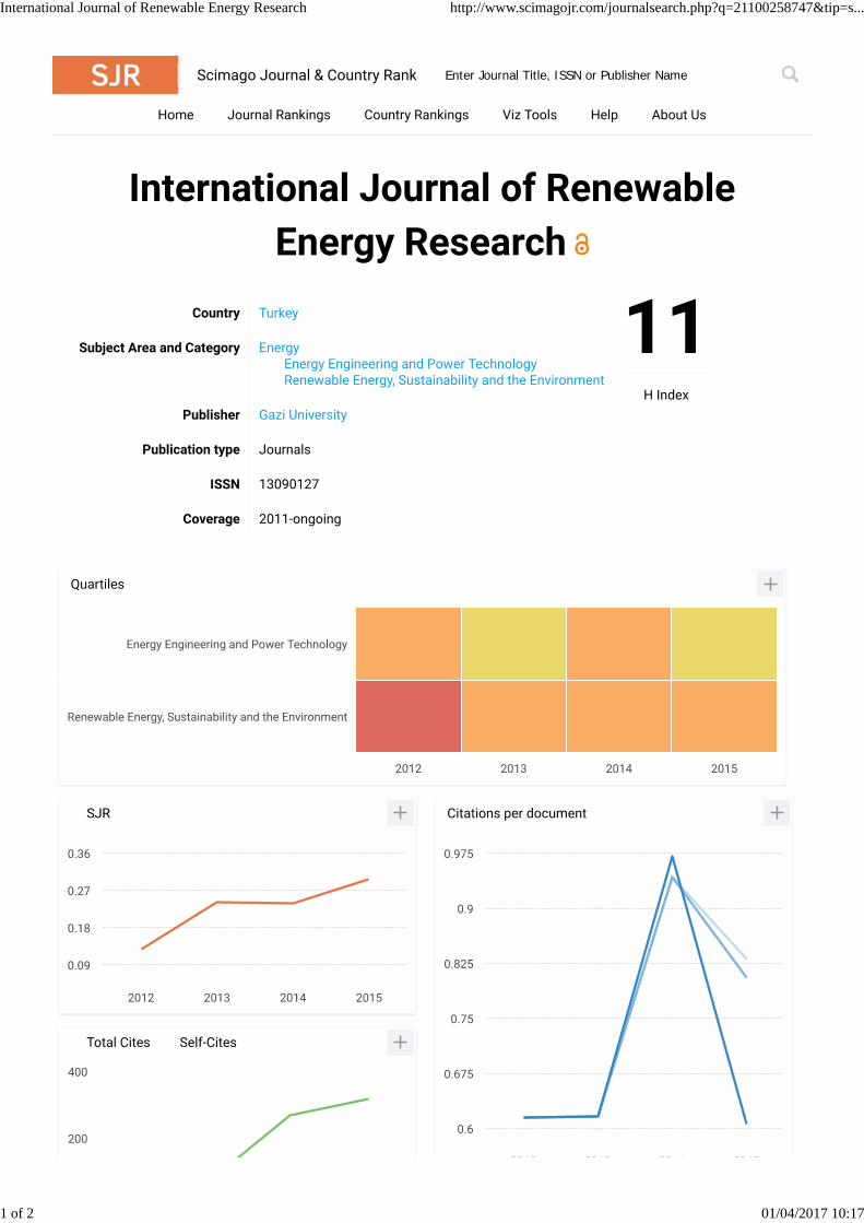
International Journal of Renewable Energy Research http://www.scimagojr.com/journalsearch.php?q=21100258747&tip=s...

2 of 2 01/04/2017 10:17

USER

Username

Password

Remember me

Login

NOTIFICATIONS

ViewSubscribe

JOURNALCONTENT

Search

Search ScopeAll

Search

BrowseBy IssueBy AuthorBy Title

FONT SIZE

INFORMATION

For ReadersFor AuthorsFor Librarians

Journal Help

HOME ABOUT LOGIN REGISTER SEARCH CURRENT

ARCHIVES ANNOUNCEMENTS

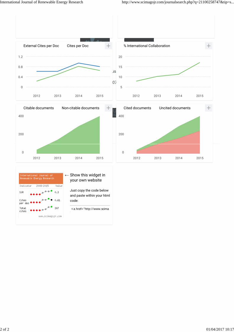
Home > Archives > Vol 7, No 1 (2017)

Vol7

DOI: http://dx.doi.org/10.1234/ijrer.v7i1

Table of Contents

Articles

Study of Integrated Rural Electrification System UsingWind-Biogas Based Hybrid System and Limited Grid SupplySystem

Dinesh Kumar Yadav, T. S. Bhatti, Ashu Verma

PDF1-11

Optimum Design and Evaluation of Solar Water Pumping Systemfor Rural Areas

Miqdam Tariq Chaichan, Ali Hussein A Kazem, Moanis M KEl-Din, Atma H. K. Al-Kabi, Asma M Al-Mamari, Hussein AKazem

PDF12-20

Effect of Rotor Speed on the Thermal Model of AFIR PermanentMagnet Synchronous Motor

Said Abd El-monem Wahsh, Jehan Hassan Shazly, Amir YassinHassan

PDF21-25

Experimental Investigation of metals and Antioxidants onOxidation Stability and Cold flow properties of PongamiaBiodiesel and its blends

Gaurav Dwivedi, Puneet Verma, mahendra pal sharma

PDF26-33

Design of Fuzzy and HBCC based Adaptive PI Control Strategy ofan Islanded Microgrid System with Solid-Oxide Fuel Cell

Subhashree Choudhury, Pravat Kumar Rout

PDF34-48

Renewable energy from the seaweed Chlorella pyrenoidosacultivated in developed systems

Souad Zighmi, Segni LADJEL, Mohamed Bilal GOUDJIL, SalahEddine BENCHEIKH

PDF49-57

Optimization of The Fins Dimensions for The Absorber with Finson a Compact Thermal Solar Collector by Entropy GenerationCriterion.

Coffi Wilfrid ADIHOU, Malahimi ANJORIN, C. AristideHOUNGAN, Christophe AWANTO, Gerard DEGAN

PDF58-67

Novel Hybrid Evolutionary Game Theory and DifferentialEvolution Solution to Generator Bidding Strategies with UnitCommitment Constraints in Energy and Ancillary ServiceMarkets

B.Durga Hari Kiran, Sailaja Kumari Matam

PDF68-79

Vol 7, No 1 (2017) http://www.ijrer.org/ijrer/index.php/ijrer/issue/view/4785074604081177

1 of 4 01/04/2017 10:14

Multi Level Inverter Based STATCOM for Grid Connected WindEnergy Conversion System

Gundala Munireddy

PDF80-87

A comparative Study And Evaluation of Improved MAF- PLLAlgorithms

mohamed mellouli, Mahmoud Hamouda, Jaleleddine Ben HadjSlama

PDF88-95

Design and Analysis of an Integrated Cuk-SEPIC Converter withMPPT for Standalone Wind/PV Hybrid System

K. Kumar, N. Ramesh Babu, K. R. Prabhu

PDF96-106

Photo-Voltaic Array Fed Transformer-Less Inverter with EnergyStorage System for Non-isolated Micro Inverter Applications

K. Mohanasundaram, P. ANANDHRAJ, V. Vimalraj Ambeth

PDF107-110

Wind-hybrid Power Generation Systems Using Renewable EnergySources- A Review

Muhammad Shahzad Aziz, Gussan Maaz Mufti, Sohaib Ahmad

PDF111-127

Performance and Cost Assessment of Three Different CrystallineSilicon PV Modules in Kuwait Environments

Adel Aldihani

PDF128-136

Dual-Axis Solar Tracker for Using in Photovoltaic SystemsCarlos Arturo Robles, Adalberto Ospino Castro, Jose CasasNaranjo

PDF137-145

Frequency Control of Micro Grid with wind Perturbations UsingLevy walks with Spider Monkey Optimization Algorithm

Kayalvizhi Selvam, D.M. Vinod Kumar

PDF146-156

High Step-Down Dual Output Light Emitting Diode DriverU. Ramanjaneya Reddy, B. L. Narasimharaju

PDF157-169

Investigate Curvature Angle of the Blade of Banki's WaterTurbine Model for Improving Efficiency by Means Particle SwarmOptimization

Lie Jasa, I Putu Ardana, Ardyono Priyadi, Mauridhi HeryPurnomo

PDF170-177

Modeling of Wind Energy Conversion System usingPSCAD/EMTDC

Asad Ashfaq

PDF178-187

Assessment of Simulation Modelling and Real-TimeMeasurements for 3.15 and 17.28 kWp Solar Photovoltaic (PV)Systems in Malaysia

Banupriya Balasubramanian, Azrul Mohd Ariffin, Samer HusamAl-Zubaidi

PDF188-199

Assessment of Effect of Load and Injection Timing on thePerformance of Diesel Engine Running on Diesel-Biodiesel Blends

Rajesh Kumar Saluja

PDF200-213

Solar Manager: Acquisition, Treatment and Isolated PhotovoltaicSystem Information Visualization Cloud Platform

David Omar Guevara, Jesús Israel Guamán, Carlos LuisVargas, Alverto Ríos Villacorta, Rubén Nogales Portero

PDF214-223

Photovoltaic Lighting System with Intelligent Control based onZigBee and Arduino

Ruben Nogales Portero, Alberto Rios

PDF224-233

Design, Dimensioning, and Installation of Isolated PhotovoltaicSolar Charging Station in Tungurahua, Ecuador

Alverto Rios Villacorta, Jesús Israel Guamán, Carlos LuisVargas, Mario Garcia Carrillo

PDF234-242

Solar photovoltaic farms suitability analysis: a Portuguesecase-study

Mário Baptista Coelho, Pedro Cabral, Sara Rodrigues

PDF243-254

An Experimental Implementation and Testing of GA basedMaximum Power Point Tracking for PV System under VaryingAmbient Conditions Using dSPACE DS 1104 Controller

Neeraj Priyadarshi, Arvind Anand, Amarjeet Sharma, Farooque

PDF255-265


2 of 4 01/04/2017 10:14

Azam, Vipin Singh, Ravi Sinha

Comparison Study of Solar Flat Plate Collector with Single andDouble Glazing Systems

H. Vettrivel, P. Mathiazhagan

PDF266-274

Simulation of Integrated Biomass Gasification-Gas Turbine-AirBottoming Cycle as an Energy Efficient System

Hassan Ali Ozgoli

PDF275-284

Remedy of Chronic Darkness & Environmental effects in YemenElectrification System using Sunny Design Web

Adel Rawea, Shabana Urooj

PDF285-291

Performance Evaluation of a Mono-Crystalline PhotovoltaicModule Under Different Weather and Sky Conditions

Nouar Aoun, Kada Bouchouicha, Rachid Chenni

PDF292-297

Performance of Zn-Cu and Al-Cu Electrodes in Seawater Batteryat Different Distance and Surface Area

Adi Susanto, Mulyono Sumotro Baskoro, Sugeng Hari Wisudo,Mochammad Riyanto, Fis Purwangka

PDF298-303

Behaviour of Biogas Containing Nitrogen on Flammability limitsand Laminar Burning Velocities

willyanto anggono

PDF304-310

Fuzzy Logic Controller based PV System Connected inStandalone and Grid Connected Mode of Operation withVariation of Load

BHUKYA KRISHNA NAICK

PDF311-322

Analysing Wind Turbine States and SCADA Data for FaultDiagnosis

Lorenzo Scappaticci, Nicola Bartolini, Alberto Garinei, MatteoBecchetti, Ludovico Terzi

PDF323-329

Improvement of Temperature Dependence of CarrierCharacteristics of Quantum Dot Solar Cell Using InN QuantumDot

Md. Abdullah Al Humayun, Sheroz Khan, A. H. M. ZahirulAlam, Mashkuri bin Yaacob, MohamedFareq AbdulMalek, MohdAbdur Rashid

PDF330-335

Technoeconomic Analysis of an Integrated GasificationCombined Cycle System as a Way to Utilise Bagasse

Stavros Michailos, David Parker, Colin Webb

PDF336-343

A Dynamic Penalty Cost Allocation Based Uncertain Wind EnergyScheduling in Smart Grid

Srikanth Konda, Lokesh Panwar, B K Panigrahi, Rajesh Kumar,Sai Goutham

PDF344-352

Modelling of Optimal Tilt Angle for Solar Collectors Across EightIndian Cities

Jims John Wessley, R Starbell Narciss, S. Singaraj Sandhya

PDF353-358

The Potential of Dark Fermentative Bio-hydrogen Productionfrom Biowaste Effluents in South Africa

Patrick Sekoai, Michael Olawale Daramola

PDF359-378

Rapid In Situ Transesterification of Papaya Seeds to Biodieselwith The Aid of Co-solvent

Elvianto Dwi Daryono

PDF379-385

Development of Customized Formulae for Feasibility andBreak-Even Analysis of Domestic Solar Water Heater

Auroshis Rout, Sudhansu S Sahoo, Sanju Thomas, Shinu MVarghese

PDF386-398

Modelling and Simulation of Natural Gas Generator and EVCharging Station: A Step to Microgrid Technology

Jakir Hossain, Nazmus Sakib, Eklas Hossain, Ramazan Bayindir

PDF399-410

Numerical evaluation of the extinction coefficient of honeycombsolar receivers

Rami Elnoumeir, Raffaele Capuano, Thomas Fend

PDF411-421


3 of 4 01/04/2017 10:14

Designing of Small Scale Fixed Dome Biogas Digester for PaddyStraw

vipan sohpal, Harmanjot Kaur, Dr Sachin Kumar

PDF422-431

A Comparative Study of Voltage Gain Tolerance in Conventionaland Three-Level LLC Converters Against Circuit Variation

Hiroyuki Haga, Hidenori Maruta, Fujio Kurokawa

PDF432-438

Output Power Loss of Photovoltaic Panel Due to Dust andTemperature

Abhishek Kumar Tripathi, M. Aruna, Ch. S. N. Murthy

PDF439-442

Modelling and Simulation of Permanent Magnet SynchronousGenerator Wind Turbine: A Step to Microgrid Technology

Jakir Hossain, Eklas Hossain, Nazmus Sakib, Ramazan Bayindir

PDF443-450

Power flow analysis incorporating renewable energy sources andFACTS devices

Suresh Velamuri, S. Sreejith

PDF451-458

Methane Hydrate Gas Storage Systems For AutomobilesSwapnil Tanaji Khot, Sanjay dnyanu Yadav

PDF459-466

Online ISSN: 1309-0127

www.ijrer.org

[email protected]; [email protected];

IJRER is cited in SCOPUS, EBSCO, WEB of SCIENCE (Thomson Reuters)


4 of 4 01/04/2017 10:14

INTERNATIONAL JOURNAL of RENEWABLE ENERGY RESEARCH L.Jasa et al., Vol.7, No.1, 2017

Investigate Curvature Angle of the Blade of Banki's

Water Turbine Model for Improving Efficiency by

Means Particle Swarm Optimization

Lie Jasa*‡, I Putu Ardana**, Ardyono Priyadi***, Mauridhi Hery Purnomo****

*Department of Electrical Engineering, Udayana University, Denpasar, Bali, Indonesia

**Department of Electrical Engineering, Udayana University, Denpasar, Bali, Indonesia

***Department of Electrical Engineering, Sepuluh Nopember Institute of Technology, Surabaya, Indonesia

****Department of Electrical Engineering, Sepuluh Nopember Institute of Technology, Surabaya, Indonesia

([email protected], [email protected], [email protected], [email protected])

‡ Corresponding Author; Lie Jasa, Department of Electrical Engineering, Kampus Unud Bukit Jimbaran Badung, Bali 80623,

Indonesia, Tel: +62 0361 703315, Fax: +62 361 703315, [email protected]

Received: 16.09.2016 Accepted:09.12.2016

Abstract-Turbines are used to convert potential energy into kinetic energy. Turbine blades are designed expertly with specific

curvature angles. The output power, speed, and efficiency of a water turbine are affected by the curvature angle of the blade

because water energy is absorbed by the blade in contact with the water flow. The particle swarm optimization (PSO)

algorithm can be used to design and optimize micro hydro turbines. In this study, the blade curvature angle in a Banki’s water

turbine model is investigated using the particle swarm optimization algorithm to obtain the highest output power, speed, and

efficiency in the water turbine. Mathematical and experimental models are employed to investigate the blade curvature angle.

The result shows that a curvature angle of 15o provides higher output power, speed, and efficiency than angles of 16o and 17o,

despite the fact that 16o is commonly used in commercial production.

Keywords blades, turbine, PSO, hydropower.

1. Introduction

Today, energy resources play an important role in

economics, politics, social life, and the sciences. This is

especially so in Indonesia where conventional energy

resources are decreasing and prices are tending to rise[1].

Renewable energy [2] sources can potentially substitute for

conventional energy resources and to smoothly solve these

problems [3]. Indonesia has many renewable energy

resources, including river water, sea water flow, tides, wind,

and geothermal and solar energies, however hydropower

plants are predominantly used for renewable energy supply

as compared with the other alternatives [4], [5], [6]. One type

of hydropower is micro-hydro power, which has become

popular since it is simpler in its design, easier and cheaper to

operate, faster to install, and has lower environmental

impacts than the others [7].

The water turbine is a simple machine usually made of

wood or steel with a fixed blade attached to a surrounding

wheel [8], [9]. This blade is driven by a stream of water

flowing around the wheel. Water pressure on the blade

produces torque on the shaft to make the wheel spin [10].

The potential energy in the accumulated water continuously

applied to the blade attached to the turbine wheel generates

kinetic energy on the turbine shaft [11]. Sometimes the water

flows vertically at the top, the middle, or the bottom of the

turbine wheel. The curvature angle of the blade is a key issue

in the energy conversion process.

One type of water turbine model is called the Banki’s

model. The theory behind the Banki’s model, written by

Mockmore and Merryfield in 1949, can be found in reference

In the Banki’s water turbine, the nozzle[12], whose cross-

sectional area is rectangular, discharges a jet into the full

width of the wheel, and is oriented at an angle of 16 degrees

to the tangent of the wheel’s periphery. More simply stated,


171

the curvature angle of the blade is 16 degrees. Based on

reference[12], the authors argued that the curvature angle is

the key for obtaining the highest possible output power,

speed, and efficiency of the water turbine.

This study explores mathematical and experimental

design models of the Banki’s water turbine to investigate the

performances resulting from 15o, 16o, and 17o blade

curvature angles. Our goal is to determine the optimal turbine

parameters for achieving the highest possible power output,

efficiency, and speed. The mathematical models explored in

our research are governed by principles of conservation of

mass, momentum, and energy, and are described in detail in

section 2. From the mathematical model we use, optimum

parameter characteristics are simulated by the particle swarm

optimization (PSO) [13], method to obtain the optimal blade

curvature angle. Then, experimental design models are used

to clarify the blade’s curvature angle obtained by PSO to

assess whether or not it yields maximum values for all of the

parameters. In order to validate the performance of the each

experimental turbine model, it was necessary to utilize the

same turbine model parameters, including wheel diameter,

thickness, material, number of blades, water discharge, and

load generators.

2. The Banki Formula

2.1 Theoretical Background

The Banki’s turbine, as described in[12], consists of a

nozzle and a turbine runner. The runner is built of two

parallel circular disks joined at their rims with a series of

curved blades. The nozzle, whose cross-sectional area is

rectangular, discharges a jet of water the full width of the

wheel, which enters the wheel at an angle of 16 degrees to

the tangent of the wheel’s periphery. The shape of the jet is

rectangular, wide, and fairly shallow. The water strikes the

blades on the rim of the wheel, as shown in Figure 1, flows

over the blade, then leaves it, passing through the empty

space between the inner rims, enters a blade on the inner side

of the rim, and is then discharged at the outer rim. The wheel

is an inward jet wheel. Since the flow is essentially radial,

the diameter of the wheel does not practically depend on the

amount of water impact, and neither does the desired wheel

breadth depend on the quantity of water.

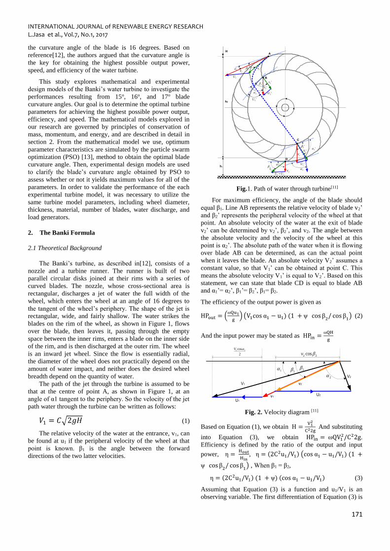
The path of the jet through the turbine is assumed to be

that at the centre of point A, as shown in Figure 1, at an

angle of α1 tangent to the periphery. So the velocity of the jet

path water through the turbine can be written as follows:

𝑉1 = 𝐶√2𝑔𝐻 (1)

The relative velocity of the water at the entrance, v1, can

be found at u1 if the peripheral velocity of the wheel at that

point is known. β1 is the angle between the forward

directions of the two latter velocities.

A

B

H

h2

h1

1 1

1U

1v1V

'2v

'2U

'2V

'2

2

'2U

C

D

'1'1V

'1U

2

1V

'1

22

21 UU 2V2v

Fig.1. Path of water through turbine[11]

For maximum efficiency, the angle of the blade should

equal β1. Line AB represents the relative velocity of blade v2’

and β2’ represents the peripheral velocity of the wheel at that

point. An absolute velocity of the water at the exit of blade

v2’ can be determined by v2’, β2’, and v2. The angle between

the absolute velocity and the velocity of the wheel at this

point is α2’. The absolute path of the water when it is flowing

over blade AB can be determined, as can the actual point

when it leaves the blade. An absolute velocity V2’ assumes a

constant value, so that V1’ can be obtained at point C. This

means the absolute velocity V1’ is equal to V2’. Based on this

statement, we can state that blade CD is equal to blade AB

and α1’= α2’, β1’= β2’, β1= β2.

The efficiency of the output power is given as

HPout = (ωQu1

g) (V1cos α1 − u1) (1 + ψ cos β

2/ cos β

1) (2)

And the input power may be stated as HPin =ωQH

g

V1 v2

V2

U2

U1

v1

1 1

2

2

2

cos 11 V

22 cosv

Fig. 2. Velocity diagram [11]

Based on Equation (1), we obtain H =V1

2

C22g And substituting

into Equation (3), we obtain HPin = ωQV12/C22g.

Efficiency is defined by the ratio of the output and input

power, η = Hout

Hin, η = (2C2u1/V1) (cos α1 − u1/V1) (1 +

ψ cos β2

/ cos β1

) , When β1 = β2,

η = (2C2u1/V1) (1 + ψ) (cos α1 − u1/V1) (3)

Assuming that Equation (3) is a function and u1/V1 is an

observing variable. The first differentiation of Equation (3) is


172

equal to zero, and is given by, u1/V1 = cos α1/2, Maximum

efficiency is given by ηmax

= (½C2) (1 + ψ)( cos 2α1 ) Based on Figure 2, the direction of V2 is not radial when u1 =

½V1α1. The water flow of the outer of rim should be radial.

Therefore, the value of u1 is given by

u1 = [C

(1+ψ)] (V1cos2α1) (4)

When there are no losses on the head due to friction in the

nozzle or the blades, ψ and C have unity values.

Variations in the nozzle roughness coefficient C is a

quadratic function, as stated at Equation (4). There are two

types of hydraulic losses from this nozzle aspect that occur

when water is striking the outer and inner peripheries. These

losses are relatively small when the blade thickness is

sufficiently thin and should not exceed the jet so, as shown in

Figure 3. Therefore, the water energy will strike the outer

and inner peripheries of the blade. The blade system can

provide the optimal blade roughness coefficient ψ, 0.98,

when the number and thickness of the blades is accurately

obtained.

r1

r2

r1

r2

a

o90'2

S2

S1

S0'1

v2'

v2'

v1'

1

2

11 sin

r

rv

t

a =r1-r

2

Fig. 3. Blade Spacing [11]

2.2 Design Construction Formula

Fig. 4. Composite velocity diagram [11]

2.2.1 Blade Angle

As stated in Figures 1 and 3, the blade angle β1 can be

calculated by u1 =1

2V1 cos α1 and tan β

1= 2 tan α1. Based

on Figures 4 and 5, the velocity of V1 ' can be obtained as

V1′ = [2gh2 + (V2

′ )2]1

2

Fig. 5. Velocity Diagram [11]

2.2.2. Width of the Radial Rim

The thickness of the entrance jet s1 for a distance of

blade t can be calculated by

s1 = t sin β1 (5)

The inner exit blade spacing s2 for a = r1 − r2 can be

obtained by s2 = t (r1/r2) where s2 = v1s1/v2′ to find the

value of β1 requires a velocity v2' influenced by the

centrifugal force, and is given by

(v1)2 − (v2′ )2 = (u1)2 − (u2

′ )2

(v2′ ) = v1 (

s1

s2) = v1 (

r1

r2) sin β

1

x2 − [1 − (v1

u1)

2

] x − (v1

u1)2sin2β

1= 0

v1

u1=

1

cos β1

where x = (r2 / r1)2

Based on Figure 6, the central angle BOC can be calculated

by

(v1)2 − (v2′ )2 = (u1)2 − (u2

′ )2

(v2′ )2 = v1 (

s1

s2) = v1 (

r1

r2) sin β

1

tan α2′ =

v2′

u2′

boC = 2 α2’ (6)

2.2.3 Wheel diameter and axial wheel breadth

The wheel diameter can be determined from Equations.

u1 = πD1N/(12)(60) and D1 = 360C(2gH)1

2 cos α1/ πN

To find the breadth of the wheel (L), where so = kD1,

Equations (26), (27) and (28) may be used.

Q = (CsoL

144) (2gH)

1

2 (7)

L = 144 Q N/862H1

2Ck(2gH)1

2 (8)

where k = 0.075 and 0.10, respectively.


173

r2

r1

a

Y2

s0

v’2

V’2

u’2

V1

v1

u1

V’1

u’1

v’1

A

B

C

D

1

'2

'2

'1'1

V2

u2=u

1

v2

22

h

h2

h1

Y1

Y

ds

BOC

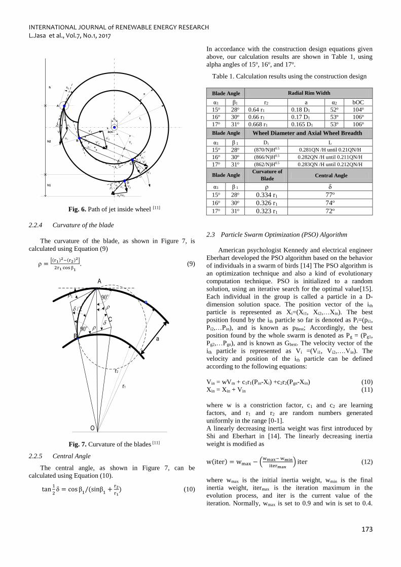
Fig. 6. Path of jet inside wheel [11]

2.2.4 Curvature of the blade

The curvature of the blade, as shown in Figure 7, is

calculated using Equation (9)

ρ =[(r1)2−(r2)2]

2r1 cos β1

. (9)

r1

r2

a

1

C

A

B

O

o90

o90

2/

Fig. 7. Curvature of the blades [11]

2.2.5 Central Angle

The central angle, as shown in Figure 7, can be

calculated using Equation (10).

tan1

2δ = cos β

1/(sinβ

1+

r2

r1) (10)

In accordance with the construction design equations given

above, our calculation results are shown in Table 1, using

alpha angles of 15o, 16o, and 17o.

Table 1. Calculation results using the construction design

Blade Angle Radial Rim Width

α1 β1 r2 a α2 bOC

15o 28o 0.64 r1 0.18 D1 52o 104o

16o 30o 0.66 r1 0.17 D1 53o 106o

17o 31o 0.668 r1 0.165 D1 53o 106o

Blade Angle Wheel Diameter and Axial Wheel Breadth

α1 β 1 D1 L

15o 28o (870/N)H0.5 0.281QN /H until 0.21QN/H



Blade Angle Curvature of

Blade Central Angle

α1 β 1 ρ δ

15o 28o 0.334 r1 77o

16o 30o 0.326 r1 74o

17o 31o 0.323 r1 72o

2.3 Particle Swarm Optimization (PSO) Algorithm

American psychologist Kennedy and electrical engineer

Eberhart developed the PSO algorithm based on the behavior

of individuals in a swarm of birds [14] The PSO algorithm is

an optimization technique and also a kind of evolutionary

computation technique. PSO is initialized to a random

solution, using an iterative search for the optimal value[15].

Each individual in the group is called a particle in a D-

dimension solution space. The position vector of the ith

particle is represented as Xi=(Xi1, Xi2,…Xin). The best

position found by the ith particle so far is denoted as Pi=(pi1,

Pi2,…Pin), and is known as pBest; Accordingly, the best

position found by the whole swarm is denoted as Pg = (Pg1,

Pg2,…Pgn), and is known as Gbest. The velocity vector of the

ith particle is represented as Vi =(Vi1, Vi2,….Vin). The

velocity and position of the ith particle can be defined

according to the following equations:

Vin = wVm + c1r1(Pin-Xi) +c2r2(Pgn-Xin) (10)

Xin = Xin + Vin (11)

where w is a constriction factor, c1 and c2 are learning

factors, and r1 and r2 are random numbers generated

uniformly in the range [0-1].

A linearly decreasing inertia weight was first introduced by

Shi and Eberhart in [14]. The linearly decreasing inertia

weight is modified as

w(iter) = wmax − (wmax− wmin

itermax) iter (12)

where wmax is the initial inertia weight, wmin is the final

inertia weight, itermax is the iteration maximum in the

evolution process, and iter is the current value of the

iteration. Normally, wmax is set to 0.9 and win is set to 0.4.


174

The following gives the design step for the improved version

of the PSO algorithm [15],[16]

3. Problem Formulation

3.1 Optimization Formula

The input power and output power equations of the

Banki turbine are affected by the value of the parameters H,

g, C, ω, ψ, α1, β1, and β2. Constant parameters, such as H, C,

and g do not change their values when optimization is

performed. The values we can optimize are the values of α1,

β1, and β2 with the goal of changing the angle of the corner to

affect the efficiency of the turbine. The equation to optimize

these parameters is as follows, by maximizing the overall

value of equations (3), (1), (4), (2) The values of influence

are the equality constraints:

V1=C(2gH)1/2

H

g

C

Hpin=WQ(V

1)2/

C22g

V1

Q

C

W

g

u1=(C/

(1+psi) V1

cos(alfa1)

C

Hpout

=((WQu1)/

g) x (V1 cos α

1-

u1).(1+ψ x ( cos

β2 / cos β

1)

W

g

Q

V1V

1

u1

Eff

Eff=

Hp

ou

t / Hp

in

V1

1

1

1

2

Fig. 8. Proposed Optimization Strategy

The inequality constraints are

cos α1 min ≤ cos α1 ≤ cos α1 max

cos β1 min ≤ cos β1 ≤ cos β1 max

cos β2 min ≤ cos β2 ≤ cos β2 max.

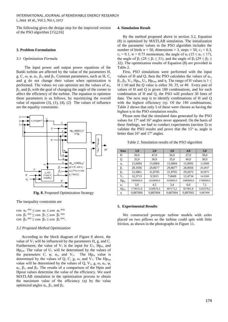
3.2 Proposed Method Optimization

According to the block diagram of Figure 8 above, the

value of V1 will be influenced by the parameters H, g, and C.

Furthermore, the value of V1 is the input for U1, Hpin, and

Hpout. The value of U1 will be determined by the values of

the parameters C, ψ, α1, and V1. The Hpin value is

determined by the values of Q, C, g, ω, and V1. The Hpout

value will be determined by the values of Q, V1, g, ω, u1, ψ,

α1, β1, and β2. The results of a comparison of the Hpin and

Hpout values determine the value of the efficiency. We used

MATLAB simulation in the optimization process to obtain

the maximum value of the efficiency (η) by the value

optimized angles α1, β1, and β2.

4. Simulation Result

By the method proposed above in section 3.2, Equation

(8) is optimized by MATLAB simulation. The initialization

of the parameter values in the PSO algorithm includes the

number of birds n = 50, dimensions = 3, steps = 50, c2 = 0.3,

c1 = 0.1, w = 0.75 momentum, the angle of α1 (15 ≤ α1 ≤ 17),

the angle of β1 (28 ≤ β1 ≤ 31), and the angle of β2 (29 ≤ β2 ≤

32). The optimization results of Equation (8) are provided in

Table 2.

First, PSO simulations were performed with the input

values of H and Q, then the PSO calculates the values of α1,

β1, β2, V1, Hpin, U1, Hpout, and η. The range of H values is 1 ≤

H ≤ 60 and the Q value is either 30, 35, or 40. Every pair of

values of H and Q is given 180 combinations, and for each

combination of H and Q, the PSO will produce 30 lines of

data. The next step is to identify combinations of H and Q

with the highest efficiency (η). Of the 180 combinations,

Table 2 shows that only 5 of these were chosen as having the

highest η in the PSO simulation results.

Please note that the simulated data generated by the PSO

values for 17o and 16o angles never appeared. On the basis of

these findings, we had to conduct experiments (section 5) to

validate the PSO results and prove that the 15o α1 angle is

better than 16o and 17o angles.

Table 2. Simulation results of the PSO algorithm

Data 1,0 2,0 3,0 4,0 5,0

H 56,0 47,0 26,0 27,0 58,0

Q 35,0 30,0 35,0 40,0 30,0

α1 15,0004 15,0004 15,0004 15,0002 15,0008

β1 28,1936 29,8677 29,8677 28,8056 29,2837

β2 31,6861 31,8705 31,8705 29,2072 30,0975

V1 10,3713 9,5015 7,0669 12,4734 14,9269

Hpin 1960000,0 1410000,0 910000,0 1080000,0 1740000,0

u1 5,0 4,5 3,4 6,0 7,1

Hpout 1738531,6 1250676,3 807173,2 957961,8 1543379,2

η 0,887006 0,887004 0,887004 0,887002 0,887000

5. Experimental Results

We constructed prototype turbine models with axles

placed on two pillows so the turbine could spin with little

friction, as shown in the photographs in Figure 11.


175

6 Cm 3 Cm 20 Cm 3 Cm 4 Cm

2 Cm 2 Cm

2,7 Cm

2 Cm

6 Cm 3 Cm 20 Cm3 Cm 4 Cm

2 Cm

2 Cm2,7 Cm

2 Cm

4 Cm 4 Cm

2 Cm

2,5 Cm

7 Cm

2.8 Cm

2.8 Cm

7 Cm

3,2 Cm

2.2 Cm

2 Cm 11 Cm2,5 Cm 2,5 Cm

2,5 Cm

16 Cm

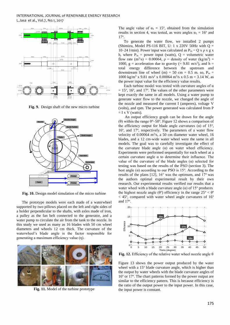
Fig. 9. Design shaft of the new micro turbine

Generator

Banki Turbin

Pully

Van Belt

Nozzle

Pump

PumpTank

Nozzle Angle

Shaft Angle

Fig. 10. Design model simulation of the micro turbine

The prototype models were each made of a waterwheel

supported by two pillows placed on the left and right sides of

a holder perpendicular to the shafts, with axles made of iron,

a pulley as the fan belt connected to the generator, and a

water pump to circulate the air from the tank to the nozzle. In

this study we used as many as 16 blades with 50 cm wheel

diameters and wheels 12 cm thick. The curvature of the

waterwheel’s blade angle is the factor responsible for

generating a maximum efficiency value (η).

Fig. 11. Model of the turbine prototype

The angle value of α1 = 15o, obtained from the simulation

results in section 4, was tested, as were angles α1 = 16o and

17o.

To generate the water flow, we installed 2 pumps

(Shimizu, Model PS-116 BIT, U: 1 x 220V 50Hz with Q =

10–24 l/min). Power input was calculated as Pin = Q x ρ x g x

h, where Pin = power input (watts), Q = volumetric water

flow rate (m3/s) = 0.00064, ρ = density of water (kg/m3) =

1000, g = acceleration due to gravity (= 9.81 m/s2), and h =

total energy difference between the upstream and

downstream line of wheel (m) = 50 cm = 0.5 m. so, Pin =

1000 kg/m3 x 9.81 m/s2 x 0.00064 m3/s x 0.5 m = 3.14 W, as

the power input value for the efficiency value results.

Each turbine model was tested with curvature angles of α

= 15o, 16o, and 17o. The values of the other parameters were

kept exactly the same in all models. Using a water pump to

generate water flow to the nozzle, we changed the angle of

the nozzle and measured the current I (amperes), voltage V

(volts), and rpm. The power generated was calculated from P

= I x V (watts).

An output efficiency graph can be drawn for the angle

(θ) within the range 0o–50o. Figure 12 shows a comparison of

the efficiency output for blade angle curvatures (α) of 15o,

16o, and 17o, respectively. The parameters of a water flow

velocity of 0.00064 m3/s, a 50 cm diameter water wheel, 16

blades, and a 12 cm-wide water wheel were the same in all

models. The goal was to carefully investigate the effect of

the curvature blade angle (α) on water wheel efficiency.

Experiments were performed sequentially for each wheel at a

certain curvature angle α to determine their influence. The

value of the curvature of the blade angles (α) selected for

testing was based on the results of the PSO (section 3). The

best angle (α) according to our PSO is 15o. According to the

results of the plans [12], 16° was the optimum, and 17o was

the authors optimal experimental result by their own

research. Our experimental results verified our results that a

water wheel with a blade curvature angle (α) of 15o produces

the highest nozzle angle (θo) efficiency in the range 25o < θo

< 45o, compared with water wheel angle curvatures of 16o

and 17o.

Fig. 12. Efficiency of the relative water wheel nozzle angle θ

Figure 13 shows the power output produced by the water

wheel with a 15o blade curvature angle, which is higher than

the output by water wheels with the blade curvature angles of

16o or 17o. The chart patterns formed by the power output are

similar to the efficiency pattern. This is because efficiency is

the ratio of the output power to the input power. In this case,

the input power is constant.

0 5 10 15 20 25 30 35 40 45 500

5

10

15

20

Theta (degree)

Eff

icie

nce

16o

17o

15o


176

Fig. 13. Power output of the water wheel vs nozzle angle θ

The RPM output can be ascribed to the nozzle angle θ.

In Figure 14 we can see that the RPM output value increases

with an increasing nozzle angle from 10o to 30o. These

results show that a 15o blade curvature angle (α) yields a

higher RPM than the water wheels with 16o and 17o blade

curvature angles (α). Other parameters were held constant in

the three experiments.

Fig. 14. RPM of the water wheel vs the nozzle angle θ

The improved results obtained with a 15o blade

curvature angle α compared with 16o and 17o blade curvature

angles α include (1) RPM value, (2) output power, (3) output

current, and (4) voltage output. We can conclude that water

wheels with a 15o blade curvature angle have higher

efficiency compared with those with 16o and 17o blade

curvature angles. Thus this study contradicts the research

results of[12], which concluded that a 16o blade curvature

angle was optimal.

6. Conclusion

The angle of the blade greatly affects water wheel

efficiency where the blade is in direct contact, such that the

thrust of water causes the wheel to spin. A 15o blade

curvature angle is shown to produce higher efficiency values

when compared with curvature angles of 16o [12]and 17o. By

utilizing the PSO algorithm to find the optimal blade

curvature angle, the water wheel is proven to generate higher

output power and higher RPM with its nozzle set at this

angle (θ) value.

The energy generated by the water wheel with a 15o

blade curvature angle proved to be higher than those with

curvature angles of 16o [12] and 17o. These results were

obtained from a mini-generator operating with a water

wheel-mounted fixed load, for which the output current and

voltage were measured. The output power of each model

were calculated, and the calculation results provide the

evidence that the 15o blade curvature angle (α) produces the

highest energy, when compared with angles of 16o and 17o.

Acknowledgements

The authors wish to convey their gratitude to the

Ministry of Ristekdikti, Indonesia, which providing financial

research Hibah Bersaing via LPPM Udayana University

2015-2016 contract No. 311-19/UN14.2/PNL.01.03/2015.

References

[1] T. H. Ching, T. Ibrahim, F. I. A. Aziz, and N. M. Nor,

“Renewable energy from UTP water supply,” in 2011

International Conference on Electrical, Control and

Computer Engineering (INECCE), 2011, pp. 142 –147.

[2] I. Ushiyama, “Renewable energy strategy in Japan,”

Renew. Energy, vol. 16, no. 1–4, pp. 1174–1179, Jan.

1999.

[3] S. Paudel, N. Linton, U. C. E. Zanke, and N. Saenger,

“Experimental investigation on the effect of channel

width on flexible rubber blade water wheel

performance,” Renew. Energy, vol. 52, pp. 1–7, Apr.

2013.

[4] A. Zaman and T. Khan, “Design of a Water Wheel For a

Low Head Micro Hydropower System,” Journal Basic

Science And Technology, vol. 1(3), pp. 1–6, 2012.

[5] L. Jasa, P. Ardana, and I. N. Setiawan, “Usaha

Mengatasi Krisis Energi Dengan Memanfaatkan Aliran

Pangkung Sebagai Sumber Pembangkit Listrik

Alternatif Bagi Masyarakat Dusun Gambuk –Pupuan-

Tabanan,” in Proceding Seminar Nasional Teknologi

Industri XV, ITS, Surabaya, 2011, pp. B0377–B0384.

[6] L. Jasa, A. Priyadi, and M. H. Purnomo, “An

Alternative Model of Overshot Waterwheel Based on a

Tracking Nozzle Angle Technique for Hydropower

Converter | Jasa | International Journal of Renewable

Energy Research (IJRER),” Ilhami Colak, vol. 4, no.

No. 4, pp. 1013–1019, Dec. 2014.

[7] T. Sakurai, H. Funato, and S. Ogasawara, “Fundamental

characteristics of test facility for micro hydroelectric

power generation system,” presented at the International

Conference on Electrical Machines and Systems, 2009.

ICEMS 2009, 2009, pp. 1 –6.

[8] G. Muller, Water Wheels as a Power Source. 1899.

[9] L. A. HAIMERL, “The Cross-Flow Turbine.”

[10] I. Vojtko, V. Fecova, M. Kocisko, and J. Novak-

Marcincin, “Proposal of construction and analysis of

turbine blades,” in 2012 4th IEEE International

Symposium on Logistics and Industrial Informatics

(LINDI), 2012, pp. 75 –80.

[11] L. Jasa, A. Priyadi, and M. H. Purnomo, “Designing

angle bowl of turbine for Micro-hydro at tropical area,”

in 2012 International Conference on Condition

Monitoring and Diagnosis (CMD), Sept., pp. 882–885.

[12] C. A. Mockmore and F. Merryfield, “The Banki Water

Turbine,” Bull. Ser. No25, Feb. 1949.

[13] M. Geethanjali, S. M. Raja Slochanal, and R. Bhavani,

“PSO trained ANN-based differential protection scheme

0 5 10 15 20 25 30 35 40 45 500

0.1

0.2

0.3

0.4

0.5

Theta(degrees)

Watt

15o

16o

17o

0 5 10 15 20 25 30 35 40 45 5070

80

90

100

110

120

130

140

Theta(degrees)

RP

M

15o

16o

17o


177

for power transformers,” Neurocomputing, vol. 71, no.

4–6, pp. 904–918, Jan. 2008.

[14] W. Dongsheng, Y. Qing, and W. Dazhi, “A novel PSO-

PID controller application to bar rolling process,” in

Control Conference (CCC), 2011 30th Chinese, 2011,

pp. 2036–2039.

[15] W. Cai, L. Jia, Y. Zhang, and N. Ni, “Design and

Simulation of Intelligent PID Controller Based on

Particle Swarm Optimization,” in 2010 International

Conference on E-Product E-Service and E-

Entertainment (ICEEE), 2010, pp. 1–4.

[16] L. Jasa, Ika Putri, A. Priyadi, and M. H. Purnomo,

“Design Optimization of Micro Hydro Turbin Using

Artifical Particel Swarm Optimization and Artificial

Neural Network,” Kursor, vol. 7, no. 3, pp. 135–144,

oktober 2014.

Documents

International Journal of Renewable Energy Research