Embed Size (px)
Citation preview

International Journal of Physical SciencesVolume 9 Number 5 16 March, 2014ISSN 1992-1950

ABOUT IJPS The International Journal of Physical Sciences (IJPS) is published weekly (one volume per year) by Academic Journals. International Journal of Physical Sciences (IJPS) is an open access journal that publishes high-quality solicited and unsolicited articles, in English, in all Physics and chemistry including artificial intelligence, neural processing, nuclear and particle physics, geophysics, physics in medicine and biology, plasma physics, semiconductor science and technology, wireless and optical communications, materials science, energy and fuels, environmental science and technology, combinatorial chemistry, natural products, molecular therapeutics, geochemistry, cement and concrete research, metallurgy, crystallography and computer-aided materials design. All articles published in IJPS are peer-reviewed.
Contact Us
Editorial Office: [email protected]
Help Desk: [email protected]
Website: http://www.academicjournals.org/journal/IJPS
Submit manuscript online http://ms.academicjournals.me/.

Editors Prof. Sanjay Misra Prof. Geoffrey Mitchell Department of Computer Engineering, School of School of Mathematics, Information and Communication Technology Meteorology and Physics Federal University of Technology, Minna, Centre for Advanced Microscopy Nigeria. University of Reading Whiteknights,
Reading RG6 6AF Prof. Songjun Li United Kingdom. School of Materials Science and Engineering, Jiangsu University, Prof. Xiao-Li Yang Zhenjiang, School of Civil Engineering, China Central South University, Hunan 410075, Dr. G. Suresh Kumar China Senior Scientist and Head Biophysical Chemistry Division Indian Institute of Chemical Biology (IICB)(CSIR, Govt. of India), Kolkata 700 032, Dr. Sushil Kumar INDIA. Geophysics Group,
Wadia Institute of Himalayan Geology,
Dr. 'Remi Adewumi Oluyinka P.B. No. 74 Dehra Dun - 248001(UC) Senior Lecturer, India. School of Computer Science Westville Campus Prof. Suleyman KORKUT University of KwaZulu-Natal Duzce University Private Bag X54001 Faculty of Forestry Durban 4000 Department of Forest Industrial Engineeering South Africa. Beciyorukler Campus 81620
Duzce-Turkey Prof. Hyo Choi Graduate School Prof. Nazmul Islam Gangneung-Wonju National University Department of Basic Sciences & Gangneung, Humanities/Chemistry, Gangwondo 210-702, Korea Techno Global-Balurghat, Mangalpur, Near District
Jail P.O: Beltalapark, P.S: Balurghat, Dist.: South Prof. Kui Yu Zhang Dinajpur, Laboratoire de Microscopies et d'Etude de Pin: 733103,India. Nanostructures (LMEN) Département de Physique, Université de Reims, Prof. Dr. Ismail Musirin B.P. 1039. 51687, Centre for Electrical Power Engineering Studies Reims cedex, (CEPES), Faculty of Electrical Engineering, Universiti France. Teknologi Mara,
40450 Shah Alam, Prof. R. Vittal Selangor, Malaysia Research Professor, Department of Chemistry and Molecular Prof. Mohamed A. Amr Engineering Nuclear Physic Department, Atomic Energy Authority Korea University, Seoul 136-701, Cairo 13759, Korea. Egypt. Prof Mohamed Bououdina Dr. Armin Shams Director of the Nanotechnology Centre Artificial Intelligence Group, University of Bahrain Computer Science Department, PO Box 32038, The University of Manchester. Kingdom of Bahrain

Editorial Board Prof. Salah M. El-Sayed Prof. Mohammed H. T. Qari Mathematics. Department of Scientific Computing. Department of Structural geology and remote sensing Faculty of Computers and Informatics, Faculty of Earth Sciences Benha University. Benha , King Abdulaziz UniversityJeddah, Egypt. Saudi Arabia Dr. Rowdra Ghatak Dr. Jyhwen Wang, Associate Professor Department of Engineering Technology and Industrial Electronics and Communication Engineering Dept., Distribution National Institute of Technology Durgapur Department of Mechanical Engineering Durgapur West Bengal Texas A&M University
College Station,
Prof. Fong-Gong Wu College of Planning and Design, National Cheng Kung Prof. N. V. Sastry University Department of Chemistry Taiwan Sardar Patel University
Vallabh Vidyanagar Dr. Abha Mishra. Gujarat, India Senior Research Specialist & Affiliated Faculty. Thailand Dr. Edilson Ferneda
Graduate Program on Knowledge Management and IT, Dr. Madad Khan Catholic University of Brasilia, Head Brazil Department of Mathematics COMSATS University of Science and Technology Dr. F. H. Chang Abbottabad, Pakistan Department of Leisure, Recreation and Tourism
Management, Prof. Yuan-Shyi Peter Chiu Tzu Hui Institute of Technology, Pingtung 926, Department of Industrial Engineering & Management Taiwan (R.O.C.) Chaoyang University of Technology Taichung, Taiwan Prof. Annapurna P.Patil,
Department of Computer Science and Engineering, Dr. M. R. Pahlavani, M.S. Ramaiah Institute of Technology, Bangalore-54, Head, Department of Nuclear physics, India. Mazandaran University, Babolsar-Iran Dr. Ricardo Martinho
Department of Informatics Engineering, School of Dr. Subir Das, Technology and Management, Polytechnic Institute of Department of Applied Mathematics, Leiria, Rua General Norton de Matos, Apartado 4133, 2411- Institute of Technology, Banaras Hindu University, 901 Leiria, Varanasi Portugal. Dr. Anna Oleksy Dr Driss Miloud Department of Chemistry University of mascara / Algeria University of Gothenburg Laboratory of Sciences and Technology of Water Gothenburg, Faculty of Sciences and the Technology Sweden Department of Science and Technology
Algeria
Prof. Gin-Rong Liu, Center for Space and Remote Sensing Research National Central University, Chung-Li, Taiwan 32001

International Journal of Physical Sciences Table of Contents: Volume 9 Number 5, 16 March, 2014
ARTICLES Numerical modeling of transients in gas pipeline 82 Mohand KESSAL, Rachid BOUCETTA, Mohammed ZAMOUM and Mourad TIKOBAINI Application of the erbium-doped fiber amplifier (EDFA) in wavelength division multiplexing (WDM) transmission systems 91 G. Ivanovs, V. Bobrovs, S. Olonkins, A. Alsevska, L. Gegere, R. Parts, P. Gavars and G. Lauks Investigation of Kenyan bentonite in adsorption of some heavy metals in aqueous systems using cyclic voltammetric techniques 102 Damaris Mbui, Duke Omondi Orata, Graham Jackson and David Kariuki

Vol. 9(5), pp. 82-90, 16 March, 2014
DOI: 10.5897/IJPS2013.3977
Article Number: 9E9923A46834
ISSN 1992 - 1950
Copyright © 2014
Author(s) retain the copyright of this article
http://www.academicjournals.org/IJPS
International Journal of Physical
Sciences
Full Length Research Paper
Numerical modeling of transients in gas pipeline
Mohand KESSAL1*, Rachid BOUCETTA2, Mohammed ZAMOUM2 and Mourad TIKOBAINI1
1Laboratoire Génie Physique des Hydrocarbures, Faculté des hydrocarbures et de la chimie, Université M’Hamed
Bougara de Boumerdés-35000- Algérie. 2Laboratoire Génie Physique des Hydrocarbures, Faculté des Sciences, Université M’Hamed Bougara de Boumerdés-
35000-Algérie.
Received 2 July 2013; Accepted 17 February, 2014
A set of equations governing an isothermal compressible fluid flow is analytically and numerically analyzed. The obtained equations are written in characteristic form and resolved by a predictor-corrector lambda scheme for the interior mesh points. The method of characteristics (MOC) is used for the boundaries. Advantages of explicit form of these schemes and the flexibility of the MOC are used for an isothermal fast transient gas flow in short pipeline. The results, obtained for a simple practical application agree with those of other methods. Key words: Gas transients, gas pipeline, lambda scheme, method of characteristics.
INTRODUCTION Gas transients equations in pipelines can be linear or generally non linear. They also may be parabolic or hyperbolic of the first or second order. As a rule, simple models are an alternative which presents a reasonable compromise between the description accuracy and the cost of solution. These models are obtained by neglecting some terms in the basic set of equations, as a result of a quantitative estimation of the particular elements of the equations for given operating conditions of the pipeline.
Several relatively new numerical schemes were tested to integrate equations of conservation. These include Godunov and TVD schemes (Leveque and Yee, 1990). These second order schemes have the advantage that shock waves problems and other discontinuities can be treated with relatively good accuracy.
In their studies, many authors have considered fast gas transients employing numerical techniques as method of characteristics (MOC) (Kameswara and Eswaran, 1993; Greyvenstein, 2001) and finite differences (Greyvenstein,
2001; Gato and Henriques, 2005), with a relatively good agreement each other. In the last decades Behbahani-Nejad and Bagheri (2010a) have used transfer functions of a single pipeline in order to develop a mathematical Simulik library. Obtained results are satisfactory with the classical methods.
With a reduced order modeling approach, Behbahani-Nejad and Shekari (2010b) have compared their results with the conventional numerical techniques for a simple gas transient example. A good agreement was observed. By the use of time space least square spectral method with a technique based on hierarchical interpolations in space and time, on numerical examples, including fast gas transients, particularly in the case of severe conditions flowing, Dorao and Fernandino (2011) have successfully handled the problem of strong shock wave.
Simulating gas transients in pipes, Ebrahimzadeha et al. (2012) have used an orthogonal collocated method technique to solve the corresponding governing equations.
*Corresponding author. E-mail: [email protected], Fax: 213 24 81 70 45.
Author(s) agree that this article remain permanently open access under the terms of the Creative Commons
Attribution License 4.0 International License
Its performances are verified and tested for two practical examples corresponding to isothermal and non isothermal cases.
In this work an, old idea, relative to a physically meaningful simples schema, have been developed by Moretti (1979), Zannetti and Colasurdo (1981) and Gabutti (1983). They are known as the lambda schemes. An important advantage of these schemes is related to
the concept of non reflecting boundary condition :a characteristics form of the boundary conditions equations is applied in order to avoid the use of the improperly reflecting technique. An explicit form of them is adapted and applied to an isothermal fast transient gas flow in short pipeline. THEORETICAL MODELING
If we consider an isothermal flow in pipeline with variable cross-
sectional area in which one dimensional continuity equation is:
0)( V
xt
(1) and momentum equation is given by :
x
zgS
D
VVfPV
xV
t
g
2)()( 2
(2) Writing equation of state for natural gas as:
ZRTP (3)
and taking into account the isothermal conditions, the acoustic wave speed becomes:
5.0ZRT
a
(4)
In the absence of field data, steady state variable distributions constitute the initial conditions. These steady state initial conditions are obtained by the use of an appropriate analytical equation (Zhou and Adewumi (1996) for Z=1:
1lln
gf
D
2
i
2D
2i
mg
f
a
(5)
Where
2
i
and Vm . This equation, which
is implicit in , is well suited for iterative method to determine
density or pressure distribution.
Kessal et al. 83
In earlier work, considering above equation set, two applications of fast and slow fluid flows have been developed by using two explicit finite-difference schemes (Kessal, 2000). Then, in the same way, a one-dimensional lambda scheme is proposed to study the first case.
NUMERICAL SCHEME
In order to analyze the gas transients phenomena in short pipelines the characteristic method is used to convert the initial partial differential equation set (1) and (2) into ordinary differential equations (Lister, 1960). The physical interpretation is that the waves travel with the speed “a”, given by the relation (4), propagating in this way the effect of the initial boundary conditions. Then the transformation of Equations (1) and (2) yields:
02
1
dx
dzgVV
D
f
dt
dV
dt
dP
a
g
(6)
02
1
dx
dzgVV
D
f
dt
dV
dt
dP
a
g
(7)
These equations are associated respectively with the following characteristics directions:
aVdt
dx (8)
aVdt
dx (9)
Using Equations (8) and (9), Equations (6) and (7) can be written as:
02
VV
D
fa
x
V
t
Va
x
P
t
P
(10)
and
0
2
VV
D
fa
x
V
t
Va
x
P
t
P
(11)
Adding Equations (10) and (11) and simplifying yields to:
0
x
V
x
Va5.0
x
P
x
P5.0
t
P
(12) Subtracting Equation (10) from Equation (11) and simplifying,
yields to: Application of an explicit lambda scheme for the above equation set needs the following transformations.
0
2
5.05.0
VVD
f
x
P
x
P
ax
V
x
V
t
V
(13)
Equations (12) and (13) are in so-called lambda form. Note that the spatial derivatives are marked with subscripts + and – to indicate the characteristic directions along which these derivatives are
84 Int. J. Phys. Sci.
approximated. Predicted values of *iV and *
iP can be obtained by
substitution of finite-difference approximations for the time derivatives into Equations (12) and (13):
x
V
x
Vta
x
P
x
PtPP j
ii 5.05.0*
(14)
j
i
j
i
j
ii VRVx
P
x
P
a
t
x
V
x
VtVV
5.0
5.0* (15)
where: D2
tfR
g
Then, the predictor–corrector scheme applied to our equation set yields to the following procedure (Gabutti, 1983). The spatial derivatives in Equations (14) and (15) are approximated as follow:
Predictor:
Part 1
x
FF
x
Fj
1i
j
i
(16)
x
FF
x
Fj
i
j
1i
(17)
Replacing the above finite-difference approximations in Equations
(14) and (15) yields the predicted values of *iV and *
iP .
Part 2
The predicted values of the time derivatives
t
P*
and
t
V*
of
Equations (12) and (13) are calculated by using the following finite difference approximations:
x
FF3F2
x
Fj
2ij1i
ji
(18)
x
FF3F2
x
Fj
2ij
1ij
i
(19)
Corrector part
By considering the following finite difference approximations and using V
* and P
* instead of V and P in Equations (12) and (13), the
corrected values of time derivatives
t
P
andt
V
can be
obtained.
x
FF
x
F*
1i*i
(20)
x
FF
x
F*i
*1i
(21)
Finally, the values of P and V at the unknown time level are
determined from the following equations:
t
P
t
Pt5.0PP
*j
i1j
i
(22)
t
V
t
Vt5.0VV
*j
i1j
i (23)
It can be noticed that above discretization is possible only at nodes 3, 4,…, N-1 as it is shown by part 2 of the predictor scheme. Then, a special treatment is needed at points near the boundaries. For this, a one sided finite-difference approximation can be used at nodes 2 and N-1.
Note that in Gabutti (1983) paper, two points finite-difference approximations was used at the nodes adjacent to the boundaries if three points were not available in the desired directions. In this study computational time interval was selected so that the Courant
stability condition was satisfied at all nodes of the mesh (Streeter and Wylie, 1969). If necessary, the time interval can be reduced in some cases.
INITIAL AND BOUNDARY CONDITIONS Initial and boundary conditions to the previous Equations (1) and (2)
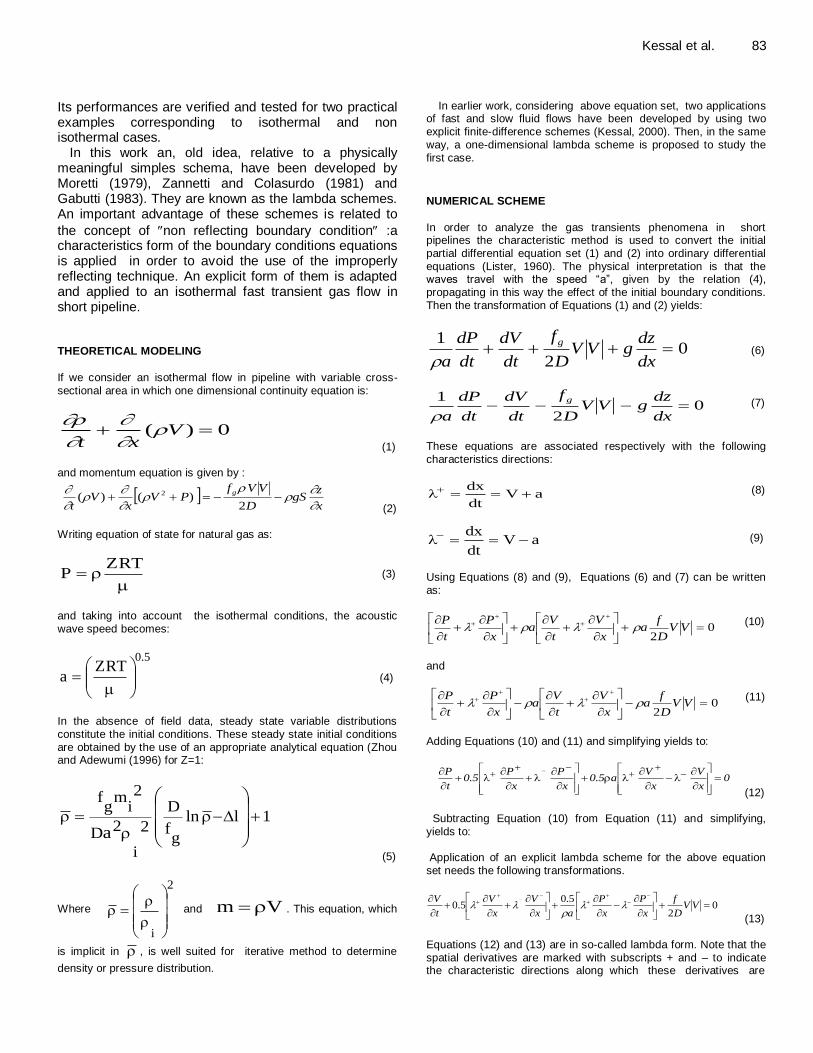
must be specified in order to obtain the appreciable solution for this differential equation set. Initial conditions of these systems are required to resolve initial pressure and velocity as a function of the position x along the pipeline. In this study they are given by the relation (8) for the pressure distribution. Boundary conditions must also be specified to obtain a unique solution. They depend on the considered cases. It is proposed in this work to treat numerically the two boundary conditions by the characteristics method. Then, integrating Equations (6) and (7) along the negative and the positive characteristics lines Equations (8) and (9) (Figure 1) yields to the following finite-difference equations:
0VRV)PP()a/1(VVj1i
j1i
j1i
1ji
j1i
j1i
1ji
(24)
0VRV)PP()a/1(VVj1i
j1i
j1i
1ji
j1i
j1i
1ji
(25)
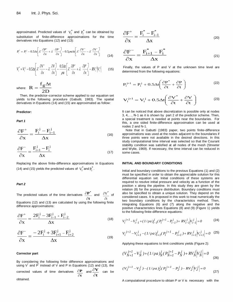
Applying these equations to limit conditions yields (Figure 2):
0VRV)PP()a/1()VV(j
Nj
Nj
N1j1N
jN
jN
1j1N
(26)
0VRV)PP()a/1()VV(j
2j
2j
21j
1j2
j2
1j1
(27)
A computational procedure to obtain P or V is necessary with the
Kessal et al. 85
Figure 1. x, t Grid for method of characteristics.
Figure 2. Characteristics at boundaries.
increments t , and equal space x. Values of fluid properties at the previous time are calculated flow from mesh i-1, i and i+1. The aforementioned stability criteria is required for:
Va
1
x
t
(28)
RESULTS AND DISCUSSION
An example concerning a gas transient in a relatively short pipeline with an impulse supply of gas mass flux at the inlet, has been simulated using the previous predictor-corrector scheme. This example is taken from Zhou and Adewumi (1996) in which solutions have been obtained, respectively, by using the method of characteristics (MOC), and, a first-order three-point
explicit Godunov scheme and a source free second-order five-point TVD scheme. A pipeline 91.44 m long, 0.609 m interior diameter and having initially a static pressure of 4136.8 kPa (with initial velocity Vi=0) with a shut downstream extremity. At time zero, upstream inflow begins to increase linearly and reaches 196 Kg/s at 0.145 s, then decreases linearly to zero again at 0.29 s, and then remains constant. The downstream end is closed. For the simulation of the above fast transient problem, the predictor-corrector lambda scheme adopts with the
characteristics method, at the boundaries, the same t imposed by the stability Criteria (28).
For numerical simulation of this example, the previous
predictor-corrector scheme adopts a grid size x=0.9144
m, t=0.811 x 10⁻³
s and C.F.L=0.312. These values can be compared with those used in the Godunov and TVD

86 Int. J. Phys. Sci.
Time (s)
Flo
w r
ate
(K
g/s
)
Fig 3. Flow rate variation at the midpoint of the pipeline
0,0 0,1 0,2 0,3 0,4 0,5 0,6 0,7 0,8
-250
-200
-150
-100
-50
0
50
100
150
200
250
TVD
MOC
Godunov
Our Model
0.0 0.1 0.2 0.3 0.4 0.5 0.6 0.7 0.8
Time (s)
Figure 3. Flow rate variation at the midpoint of the pipeline.
0,0 0,2 0,4 0,6 0,8
4,1e+6
4,2e+6
4,2e+6
4,3e+6
4,3e+6
4,4e+6
4,4e+6
4,5e+6
4,5e+6
Time (s)
Pre
ssure
(P
a)
Fig 4. Pressure response at the inlet of the pipe.
TVD
MOC
Goudunov
Our model
4.5e+6
4.5e+6
4.4e+6 4.4e+6 4.3e+6
4.3e+6
4.2e+6 4.2e+6 4.1e+6 0.0 0.2 0.4 0.6 0.8
Time (s)
Figure 4. Pressure response at the inlet of the pipe.
Schemes (19) respectively: x=0.9144 m, t=0.09144 x
10-3
s and C.F.L=0.0348; x=0.9144 m, t=0.9 x 10⁻³
s and C.F.L=0.348. Some numerical results are illustrated by the following figures. It shown a time evolution rate of the gas (Figure 3) at midpoint of the gas line (x=0.5*L), where our results are compared with those obtained by Zhou and Adewumi
(1996). Good agreement between
them can be observed. The gas flow rate fronts are
completely solved within the first 0.8 s. The behaviour of gas flow rate evolution at the midpoint of the pipeline is the result of reflected pressure impulse at the upstream end of the pipe.
A comparison of the predicted pressure (by the present model) at the inlet of the pipeline (x/L=0) with the reported data as shown in Figure 4. Again, relatively good agreement between the predicted results and the

Kessal et al. 87
0.0 0.1 0.2 0.3 0.4 0.5 0.6 0.7 0.8
Time (s)
Time (s)
Pre
ssu
re (
Pa)
Figure 5. Pressure response at the inlet of the pipeline.
0,0 0,4 0,8 1,2 1,6 2,0 2,4
4,0e+6
4,2e+6
4,4e+6
4,6e+6
4,8e+6
TVD scheme
Godunov scheme
Our Model
4.8e+6
4.6e+6
4.4e+6
4.2e+6
4.0e+6
0.0 0.4 0.8 1.2 1.6 2.0 2.4
Time (s) Figure 5. Pressure response at the inlet of the pipeline.
0.0 0.1 0.2 0.3 0.4 0.5 0.6 0.7 0.8
Time (s)
4.60e+6 4.50e+6 4.40e+6 4.30e+6
4.20e+6 4.10e+6
0.0 0.2 0.4 0.6 0.8
Time (s)
Figure 6. Pressure response at the outlet of the pipe.
reported data is obtained. It can be noticed that duration of the pressure pulse of the peak is the same. Pressure wave is maintained and captured during the first 0.80 s. The pressure wave fronts are reproduced during 2.4 s, without any loss of accuracy (Figure 5). Slight differences with an other methods can be due to some simplifications introduced by Zhou and Adewumi (1996), that is, the value of the friction losses coefficient. A comparison, as regards the pressure at the outlet point of the pipeline
(x/L=1), between obtained numerical results and the reported data is shown in Figure 6. Good agreement can be noticed. At the outlet of the pipeline, the pressure wave fronts are completely resolved within the first 0.8 s.
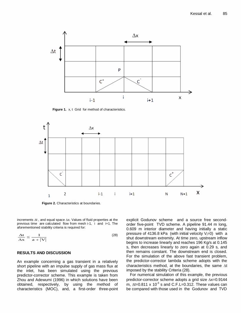
In order to check the numerical method described herein, the pressure evolution has been calculated for time close to the end of the transient phenomenon. It is shown in Figure 7 that agreement is satisfactory. This indicates that the method described in the previous
88 Int. J. Phys. Sci.
0.0 0.1 0.2 0.3 0.4 0.5 0.6 0.7 0.8
Time (s)
4.6e+6
4.5e+6
4.4e+6
4.3e+6 4.2e+6
4.2e+6
4.1e+6
4.0e+6
20.0 20.5 21.0 21.5 22.0 22.5 23.0
Time (s)
Figure 7. Pressure response at the inlet of the pipe.
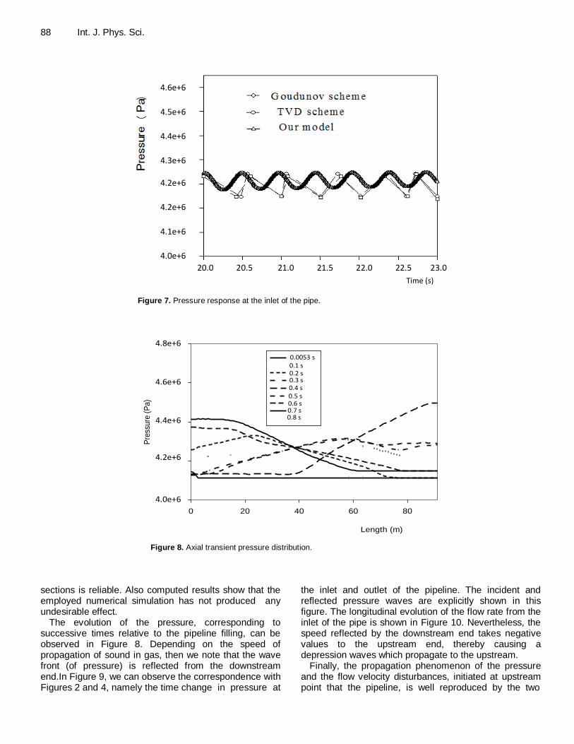
Figure 8. Axial transient pressure distribution
Length (m)
0 20 40 60 80
Pre
ssure
(P
a)
4,0e+6
4,2e+6
4,4e+6
4,6e+6
4,8e+6
0,0053 s
0,1 s
0,2 s
0,3 s
0,4 s
0,5 s
0,6 s
0,7 s
0,8 s
0.0 0.1 0.2 0.3 0.4 0.5 0.6 0.7 0.8
Time (s)
4.8e+6
4.6e+6
4.4e+6
4.2e+6
4.0e+6
20.0 20.5 21.0 21.5 22.0 22.5 23.0
Time (s)
0.0 0.1 0.2 0.3 0.4 0.5 0.6 0.7 0.8
Time (s)
0.2 s 0.1 s 0.0053 s
0.3 s 0.4 s 0.5 s 0.6 s 0.7 s 0.8 s
Figure 8. Axial transient pressure distribution.
sections is reliable. Also computed results show that the employed numerical simulation has not produced any undesirable effect.
The evolution of the pressure, corresponding to successive times relative to the pipeline filling, can be observed in Figure 8. Depending on the speed of propagation of sound in gas, then we note that the wave front (of pressure) is reflected from the downstream end.In Figure 9, we can observe the correspondence with Figures 2 and 4, namely the time change in pressure at
the inlet and outlet of the pipeline. The incident and reflected pressure waves are explicitly shown in this figure. The longitudinal evolution of the flow rate from the inlet of the pipe is shown in Figure 10. Nevertheless, the speed reflected by the downstream end takes negative values to the upstream end, thereby causing a depression waves which propagate to the upstream.
Finally, the propagation phenomenon of the pressure and the flow velocity disturbances, initiated at upstream point that the pipeline, is well reproduced by the two

Kessal et al. 89
4,0e+6
4,1e+6
4,2e+6
4,3e+6
4,4e+6
4,5e+6
4,6e+6
0,0
0,2
0,4
0,6
0,8
020
4060
80
Pre
ssu
re (
Pa
)
Tim
e (s
)
Length (m)
Figure 9. 3D Gas transients between the inlet and outlet
4.6e+6 4.5e+6
4.4e+6
4.3e+6
4.2e+6
4.1e+6
4.0e+6
0.0
0.2
0.4
0.6
0.8
Figure 9. 3D Gas transients between the inlet and outlet.
Figure 10. Axial transient velocity
Length (m)
0 20 40 60 80
Velo
city
(m/s
)
-20
0
20
40
60
0,005 s
0,1 s
0,2 s
0,3 s
0,4 s
0,5 s
0,6 s
0,7 s
0,8 s
Time (s)
0.2 s 0.1 s 0.005 s
0.3 s 0.4 s 0.5 s
0.6 s 0.7 s 0.8 s
Figure 10. Axial transient velocity.
forms of difference schemes, that is, a second order scheme for the interior points and a method of
characteristics for the extremities. The gas transients are contained in a very comprehensive and convenient.

90 Int. J. Phys. Sci. CONCLUSION The numerical methods presented in this study allow to calculate the propagation of pressure or velocity disturbances from one boundary of a gas pipeline. We have shown that the explicit lambda type of finite difference scheme presents an acceptable computational time. Also, the obtained results have shown that the accuracy of the previous scheme is comparable to the one of high resolution scheme for the considered examples. Nomenclature S: cross-sectional area of pipeline, vector; a :isothermal speed of sound; D: pipeline diameter; fg: gas friction factor; g: gravitational acceleration; N: number of space
intervals; : molecular gas weight; p: pressure; R:
universal gas constant or D
tfR
g
2
; T: time; l, L: length;
T: absolute gas temperature; V: gas velocity; X: axial
co-ordinate , L; Z: compressibility factor or elevation; :
gas density;i: inlet gas density; t: uniform time step;
x: uniform grid size. Subscripts g: gas; i: inlet, node. Conflict of Interests
The author(s) have not declared any conflict of interests. REFERENCES Behbahani-Nejad M, Bagheri A (2010a). The Accuracy and Efficiency of
a MATLABSimulink Library for Transient Flow Simulation of Gas Pipelines and Networks. J. Pet. Sci. Eng. 70:256–265. http://dx.doi.org/10.1016/j.petrol.2009.11.018
Behbahani-Nejad M, Shekari Y (2010b). The accuracy and efficiency of a reduced-order model for transient flow analysis in gas pipelines. J. Pet. Sci. Eng. 73:13-19. http://dx.doi.org/10.1016/j.petrol.2010.05.001
Dorao CA, Fernandino M (2011).Simulation of transients in natural gas pipelines. J. Nat. Gas Sci. Eng. 3(1):319-364. http://dx.doi.org/10.1016/j.jngse.2011.01.004
Edris E, Mahdi NS, Bahamin B (2012). Simulation of transient gas flow using the orthogonal collocation method. Chem. Eng. Res. Des. P. 90.
Gabutti B (1983). On two Upwind Finite-Difference Schemes for Hyperbolic Equations in Non-Conservative Form. Comput. Fluids. 11(3):207-230. http://dx.doi.org/10.1016/0045-7930(83)90031-2
Gato LMC, Henriques JCC (2005). Dynamic behavior of high pressure natural gas flow in pipelines. Int. J. Heat Mass Transf. 26:817-825.
Greyvenstein GP (2001). An implicit method for the analysis of transient flows in pipe networks. Int. J. Numer. Methods Eng. 53(5):1127-1143.
http://dx.doi.org/10.1002/nme.323 Kameswara R, Eswaran K (1993). On the Analysis of Pressure
Transients in Pipelines., Int. J. Pres. Ves. Piping. 56:107-129.
http://dx.doi.org/10.1016/0308-0161(93)90120-I
Kessal M (2000). Simplified Numerical Simulation of Transients in Gas
Networks, Chemical. Eng. Res. Design, Vol. 78, Part A. http://dx.doi.org/10.1205/026387600528003
Leveque RJ, Yee HC (1990). A study of Numerical Methods for Hyperbolic conservation laws with stiff source terms. J. Comp. Phys. 86:187-210. http://dx.doi.org/10.1016/0021-9991(90)90097-K
Lister M (1960). The Numerical Solution of Hyperbolic Partial Differential Equations By the Method of Characteristics, in Ralston, A., and Wilf, H.S., Eds, Mathematical Methods for Digital Computers,
Wiley, New York, pp.165-179.
Moretti G (1979). The -Schemes, Computers & Fluids. 7(4):191-205.
http://dx.doi.org/10.1016/0045-7930(79)90036-7 Streeter VL, Wylie EB (1969). Natural gas pipeline transients, SPEJ. pp.
357-364.
Zannetti L, Colasurdo G (1981). Unsteady Compressible Flow: A Computational Method Consistent with the physical Phenomenon. AIAA J. 19:951-956.
Zhou JJ, Adewumi MA (1996). Simulation of Transients in Natural Gas pipelines, SPEJ. pp. 202-208.
Vol. 9(5), pp. 91-101, 16 March, 2014
DOI: 10.5897/IJPS2013.4066
Article Number: 770DF9D46836
ISSN 1992 - 1950 © 2014
Copyright © 2014
Author(s) retain the copyright of this article
http://www.academicjournals.org/IJPS
International Journal of Physical
Sciences
Full Length Research Paper
Application of the erbium-doped fiber amplifier (EDFA) in wavelength division multiplexing (WDM)
transmission systems
G. Ivanovs, V. Bobrovs, S. Olonkins, A. Alsevska, L. Gegere, R. Parts, P. Gavars and G. Lauks
Institute of Telecommunications, Riga Technical University, Azenes Str. 12, Rīga, LV-1048, Latvia.
Received 7 November, 2013; Accepted 19 February, 2014
In the work, characteristics of the erbium-doped fiber amplifier (EDFA) are investigated. The amplification and noise figure dependences on different EDFA parameters in a 2.5 Gbit/s one-channel WDM transmission system are simulated and measured. Additionally, simulation of a four-channel 2.5 Gbit/s WDM system containing in-line amplifiers of the type was done in order to investigate the EDFA performance in multichannel systems. Almost identical results obtained for both the simulation model and the experimental system are indicative of high accuracy of the simulation. It is shown that the EDFA amplification depends on such parameters as the signal power, wavelength, EDF length, and configuration of the pump laser. Key words: Wavelength division multiplexing (WDM), erbium-doped fiber amplifier (EDFA).
INTRODUCTION
The capacity of fiber optical communication systems has undergone enormous growth during the last few years in response to huge capacity demand for data transmission (Cisco Systems, 2010). With the available WDM components, commercial systems transport more than 100 channels over a single fiber (Bobrovs et al., 2009). Hence, the installed systems of the type can be upgraded many times without adding a new fiber, which makes it possible to build inexpensive WDM systems with much greater capacity (Azadeh, 2009). Increasing the number of channels in such systems will eventually result in the usage of optical signal demultiplexing components with greater values of optical attenuation. Additionally to this, when transmitted over long distances, the optical signal is highly attenuated, and, therefore, to restore the optical power budget it is necessary to implement optical signal
amplification. At the choice of signal amplification method for the wavelength division multiplexing (WDM) systems the preference is given to the class of erbium-doped fiber amplifiers (EDFAs). These amplifiers are low-noise, almost insensitive to polarization of the signal and can be relatively simply realized (Dutta et al., 2003). Besides providing gain at 1550 nm, in the low-loss window of a silica fiber such amplifier allows achieving such gain in a band wider than 4000 GHz. To ensure the required level of amplification over the frequency band used for transmission it is highly important to choose the optimal configuration of the EDFAs, as the flatness and the level of the obtained amplification, and the amount of EDFA produced noise are highly dependent on each of the many parameters of the amplifier. In this article the authors investigate the behavior of EDFAs depending on
*Corresponding author. E-mail: [email protected]. Tel: +371 26757946.
Author(s) agree that this article remain permanently open access under the terms of the Creative Commons
Attribution License 4.0 International License

92 Int. J. Phys. Sci.
Figure 1. Scheme of the erbium-doped fiber amplifier (Dutta et al., 2003).
Figure 2. Schematic diagram of erbium ion energy levels and the
spontaneous lifetimes of excited levels.
such amplifier parameters as input optical power, power and wavelength of the pumping radiation, length of the EDF and the achieved level of erbium population inversion. MAIN COMPONENTS OF ERBIUM-DOPED FIBER AMPLIFIER
The amplifier under consideration consists of a fiber having a silica glass host core doped with active Er ions as the gain medium (Becker et al., 1999). The erbium-doped fiber is usually pumped by semiconductor lasers at 980 nm or 1480 nm. The signal is amplified while propagating along a short span of such a fiber (Agrawal, 2002). A simplified scheme of the EDFA is displayed in Figure 1.
In the scheme, the amplifier is pumped by a semiconductor laser, which is complemented with a wavelength selective coupler (also known as the WDM coupler) which combines the pump laser light with the signal light. The pump light propagates either in the same direction as the signal (co-propagation) or in the opposite direction (counter-propagation). Optical isolators are used to prevent oscillations and excessive noise due to unwanted reflections (Mukherjee, 2006).
The main condition that should be fulfilled to ensure the optical power transfer to the signal is that the
erbium atoms are to be in the excited state. The excitation is performed by a powerful pumping laser with a corresponding radiation wavelength of 980 nm or 1480 nm. The pump laser diode, as shown in Figure 1, generates a high-power beam of light at such a wavelength that the erbium ions absorb it and reach the excited state. When the photons belonging to the signal meet the excited erbium atoms, these atoms give up a portion of their energy to the signal and return to a lower-energy state (Figure 2). Erbium gives up its energy in the form of additional photons which have exactly the same phase and direction as the signal being amplified. So the signal is amplified along its direction of travel only. The pumping laser power is usually controlled via feedback (Trifonovs et al., 2011).
The gain spectrum of EDFAs is determined by the molecular structure of the doped fiber, and is strictly wavelength-dependent. The main disadvantage of EDFAs is that even though their gain spectrum bandwidth can reach 4000 GHz, it is highly wavelength dependent, and obtaining relatively flat gain spectrum over a wide wavelength band can become complicated. This problem can be solved by supplementing the EDFA with an another type of amplifier, that is, distributed Raman amplifier, the gain spectrum of which can be varied in a way to obtain flat overall gain over the desired wavelength band. Such solution will also increase the achievable level of amplification, but one must always
Ivanovs et al. 93
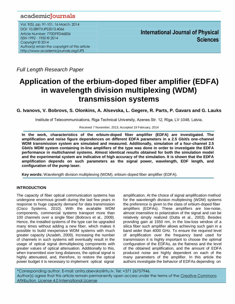
Figure 3. Simplified optical network for studying EDFA parameters.
take into account the accumulating impact of fiber nonlinearity (Bobrovs et al., 2013).
Due to the wavelength dependency of the gain, EDFAs can ensure amplification of individual channels and, therefore, no cross-gain saturation will occur during the process of amplification. Due to a relatively long spontaneous carrier lifetime in silica fibers, this allows achieving high gain for a weak signal with low noise figure, which represents the difference in signal-noise ratio at the input and output of the device under consideration (Bobrovs et al., 2013).
REALIZATION OF EDFA AND EXPERIMENTAL MEASUREMENT SCHEME
Experimental results for investigation of EDFA performance dependence on the parameters of the amplifier were obtained by introducing a simulation model of a single channel optical transmission system, and comparing the obtained results with results obtained in a real-life experiment. Afterwards a simulation model of a 4 channel WDM transmission system was introduced to assess the performance of the EDFA, when it is used as an in-line optical amplifier in a multichannel WDM system.
Simulation of the EDFA amplifier was done with the help of RSoft Design Group OptSim™ software. This software offers two simulation modes: The sample mode and the block mode. The latter was used since it allows observing and studying the EDFA intrinsic processes: The pump power and amplification propagation as well as appearance of ASE (amplified spontaneous emission) noise and its evolution along the fiber (OptSim User Guide, 2008).
For studying the EDFA parameters and their impact on the total signal amplification and the ASE noise increase, a one-channel optical link scheme was developed. As shown in Figure 3, the scheme contains three main sections: transmitter, amplifier, and receiver sections.
The transmitter section consists of a binary data source and a non-return-to-zero (NRZ) on-off keying optical
signal source. The data source generates 2.5 Gbit/s data flow. The NRZ version was chosen because it is the most popular code method used in optical transmission systems and due to its comparatively simple realization (Bobrovs et al., 2011). The signal wavelength λ = 1535 nm corresponds to the C optical band (Mukherjee, 2006). The power of optical signal was set to -30 dBm (a typical value for a weak signal to reach the amplifier).
The amplifier section consists of a physical model of the EDFA which, in turn, includes an optical multiplexer and a 980 nm co-propagating continuous wave pumping laser. To simplify the simulation process and to focus on the EDFA performance, transmission fiber was not included in this simulation scheme. Other EDFA parameters: the erbium-doped fiber (EDF) length l was 14 m, and the pumping laser power was P = 40 mW.
The receiver section consists of a PIN photodiode, a preamplifier and a Bessel’s filter, grouped together in one receiver (Bobrovs et al., 2010). The measuring elements were placed before and after the amplifier in order to detect changes of parameters of the amplified signal that occur in the EDF (Udalcovs et al., 2011).
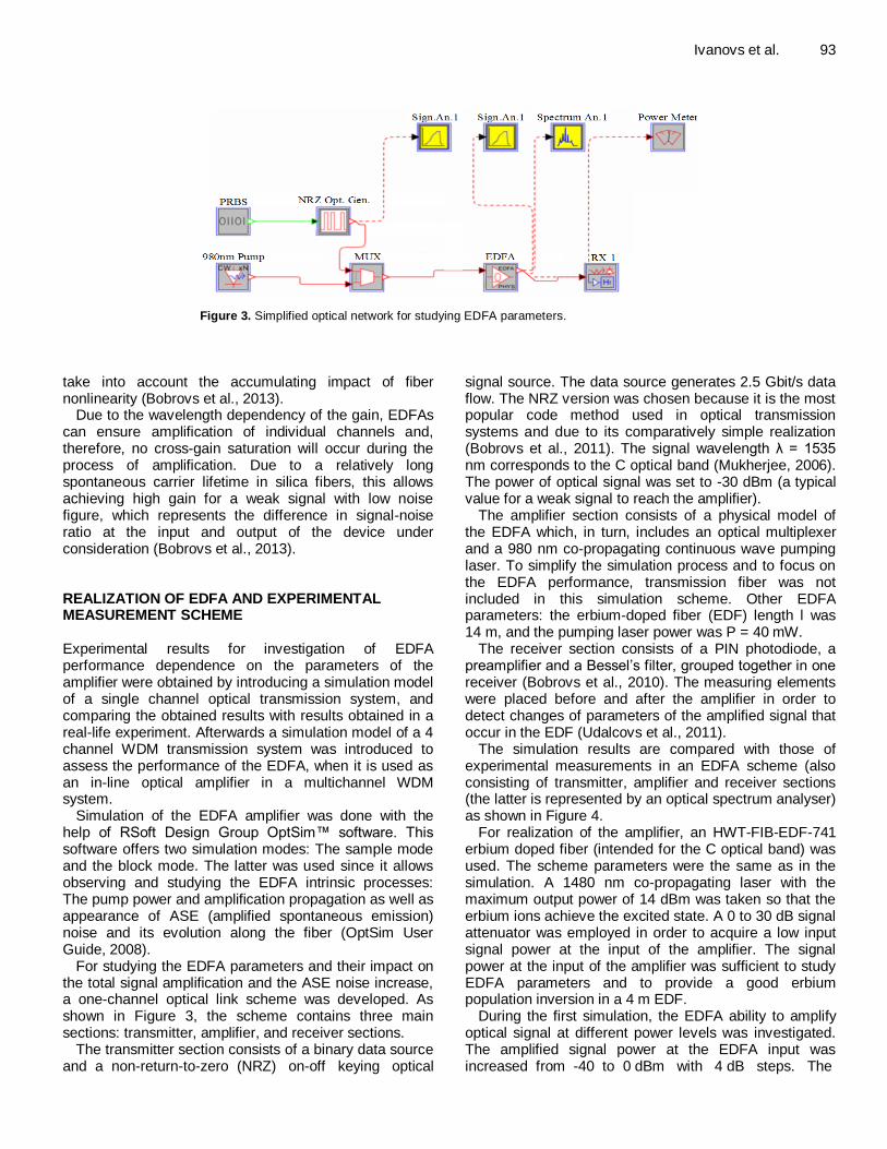
The simulation results are compared with those of experimental measurements in an EDFA scheme (also consisting of transmitter, amplifier and receiver sections (the latter is represented by an optical spectrum analyser) as shown in Figure 4.
For realization of the amplifier, an HWT-FIB-EDF-741 erbium doped fiber (intended for the C optical band) was used. The scheme parameters were the same as in the simulation. A 1480 nm co-propagating laser with the maximum output power of 14 dBm was taken so that the erbium ions achieve the excited state. A 0 to 30 dB signal attenuator was employed in order to acquire a low input signal power at the input of the amplifier. The signal power at the input of the amplifier was sufficient to study EDFA parameters and to provide a good erbium population inversion in a 4 m EDF.
During the first simulation, the EDFA ability to amplify optical signal at different power levels was investigated. The amplified signal power at the EDFA input was increased from -40 to 0 dBm with 4 dB steps. The
94 Int. J. Phys. Sci.
Figure 4. Experimental scheme of EDFA measurements.
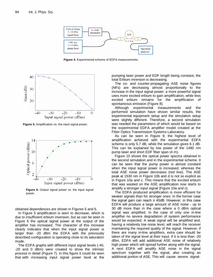
Figure 5. Amplification vs. the input signal power.
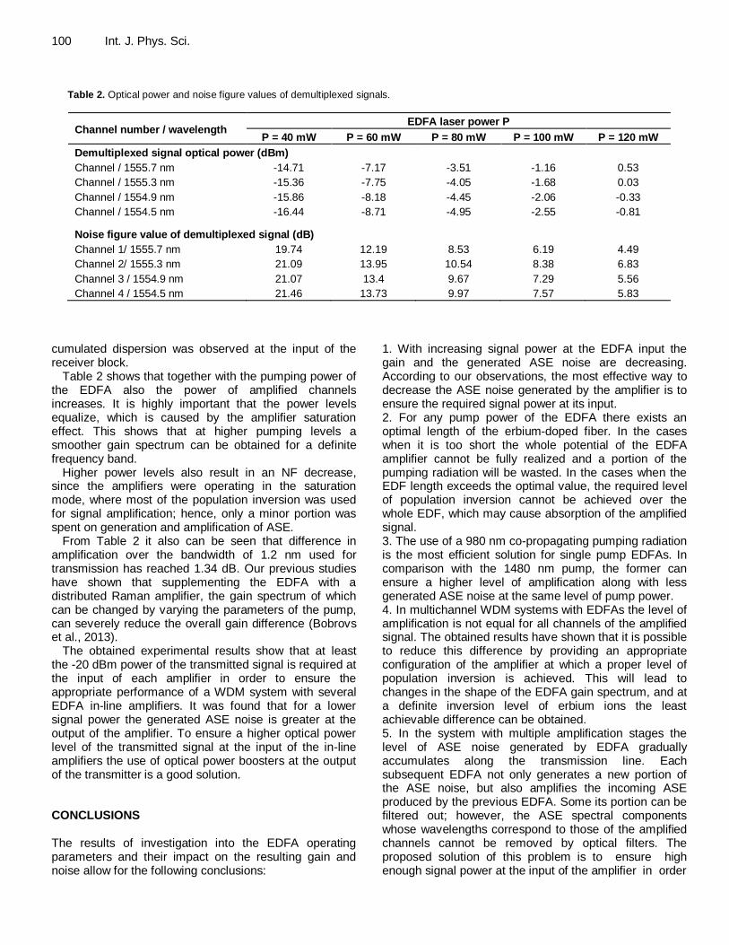
Figure 6. Output signal power vs. the input signal
power.
obtained dependences are shown in Figures 5 and 6.
In Figure 5 amplification is seen to decrease, which is due to insufficient erbium inversion, but as can be seen in Figure 6 the optical signal power at the output of the amplifier has increased. The character of this increase clearly indicates that when the input signal power is larger than -20 dBm the EDFA with the previously described configuration is operating close to its saturation mode.
The EDFA graphs with different input signal levels (-40, -20 and 0 dBm) were created to show the intrinsic process in detail (Figure 7). In this figure it could be seen that with increasing input signal power level at the
pumping laser power and EDF length being constant, the total Erbium inversion is decreasing.
The co- and counter-propagating ASE noise figures (NFs) are decreasing almost proportionally to the increase in the input signal power: a more powerful signal uses more excited erbium to gain amplification, while less excited erbium remains for the amplification of spontaneous emission (Figure 8).
Although experimental measurements and the performed simulation have shown similar results, the experimental equipment setup and the simulation setup were slightly different. Therefore, a second simulation was needed the parameters of which would be based on the experimental EDFA amplifier model created at the Fiber Optics Transmission Systems Laboratory.
As can be seen in Figure 9, the highest level of amplification achieved with the experimental EDFA scheme is only 5.7 dB, while the simulation gives 6.1 dB. This can be explained by low power of the 1480 nm pump laser and short EDF fiber span (4 m).
Figure 10 shows the optical power spectra obtained in the second simulation and in the experimental scheme. It can be seen that the pump power is almost constant when the input signal power is increased, whereas the total ASE noise power decreases (red line). The ASE peak at 1530 nm in Figure 10b and d is not so explicit as in Figure 10a and c. This means that the excited erbium that was wasted on the ASE amplification now starts to amplify a stronger input signal (Figure 10a and c).
The EDFA produced amplification is more efficient for weaker signals than for stronger ones: In the former case the signal gain can reach ≥ 40dB. However, in this case EDFA will produce a large amount of ASE noise - up to 30 dB more than in the case where a 0 dBm optical signal was amplified. In the case of only one in-line amplifier no severe degradation of system performance would be expected. A weak signal will be amplified and, having a relatively low noise level, will reach the receiver maintaining the required quality of the signal. However, if there are many in-line amplifiers, extra care should be taken of the signal level at their input. If it is less than -20 dBm, EDFA will add additional ASE noise of relatively high power which will spread further along with the signal. A next EDFA will amplify ASE noise in the signal spectrum together with the signal, also creating an additional portion of ASE. This will cause severe signal-

Ivanovs et al. 95
Figure 7. Excited erbium state densities at different input signal levels: -40 dBm (a), -20 dBm (b) and 0 dBm (c). N2 – excited state, N1 – ground state.
Figure 8. Co-propagating ASE generation at different input signal levels: -40 dBm (a), -20 dBm (b) and 0 dBm (c).
to-noise ratio degradation.
In the second experiment, the dependences of amplification and noise on the EDF length (varied from 5 to 30 m with a 5 m step) were investigated. Other parameters were kept constant. The obtained results are shown in Figure 10a and b.
The maximum amplification with chosen parameters was achieved for the 15 m long EDF. In turn, the noise
figure (the relation of signal-to-noise ratio before and after amplification) increased with the EDF length.
To analyze the dependences shown in Figure 11, EDFA internal erbium density state graphs were obtained (Figure 12). At the EDF length of 5m (Figure 12a) all erbium is in excited state. The signal obtains only half of the achievable gain in such a short fiber span; in turn, the ASE noise level is quite low. This shows that the EDFA is

96 Int. J. Phys. Sci.
Figure 9. EDFA amplification vs. the input signal power: simulation (a), and measurements (b).
Figure 10. Power spectra at the EDFA output. Simulation – input signal power -22
dBm (a), 6 dBm (b),measurement – input signal power -21.66 dBm (c), 6 dBm (d).
operating in the saturation mode, with almost 100% inversion and the amplification being homogeneous throughout the EDF.
When the length of the EDF was increased to 20 m (Figure 12b) at the 15th meter of the EDF signal amplification achieves its maximum, while the amount of excited erbium ions is approaching that of the base state erbium − from this point on the EDFA does not amplify the signal. Counter-propagating ASE also leads to the inversion decrease at the beginning (first 0-5 m) of the EDF fiber. In the case of a 30 m long EDF (Figure 12c) starting from 15 m and to the end of the fiber, erbium inversion was lower than 50% and signal absorption took
place. In this case the EDF absorbs the signal together with ASE noise.
During the third simulation, different pumping laser configurations were analyzed. The optical power, direction and wavelength of the pump were changed, while other simulation parameters were kept constant. Aggregated information is placed in Table 1. To provide the same amplification, a 1480 nm laser requires longer erbium-doped fiber than a 980 nm one. In the case of 980 nm laser, exciting erbium to a higher energy state requires less energy than in the case of 1480 nm laser at the same laser power, so the use of 980 nm wavelength will ensure a higher level of amplification. At the same

Ivanovs et al. 97
Figure 11. Amplification vs. EDF length (a), noise figure vs. EDF length (b).
Figure 12. Densities of erbium ion states. EDF length: 5 m (a), 20 m (b) and 30 m
(c). N2 – excited state, N1 – ground state.
time, using 1480 nm lasers a higher laser power can be applied and even greater output signal level can be achieved. Combined laser pumping, as was expected, gave the largest signal amplification since it provided larger erbium inversion along the erbium-doped fiber length.
The lowest NF was achieved in the case of 980 nm co-propagation laser. The highest NF was observed in the case of 1480 nm counter-propagating pumping radiation. Combined pumping showed the best results because it provides high erbium inversion along EDF fiber, and, therefore, the highest gain of all observed pumping configurations and a good noise ratio. The 1480 nm laser allowed achieving a high level of amplification, however produced more noise. Therefore, in a two-laser setup the 1480 nm laser is better to connect in the counter-
propagating direction. REALIZATION OF A 2.5 GBIT/S WDM SYSTEM WITH IN-LINE EDFA
The WDM transmission system under attention was composed of four 2.5 Gbit/s WDM channels with 50 GHz channel spacing. The line length was 400 km. The impact of dispersion was compensated with the help of a dispersion compensating fiber (DCF). The simplified (does not include all the measurement components) simulation scheme of the 4 channel DWDM transmission system under attention is displayed in Figure 13. Each channel has its own corresponding transmitter and receiver. In the transmitter block the logical signal was

98 Int. J. Phys. Sci. Table 1. Simulation results for -30 dBm 1535 nm signal at the input of EDFA.
Pumping laser Laser power,
mW
Output signal,
dBm
Co-prop. ASE, dBm
Counter-prop. ASE, dBm
Co-prop. ASE at 1535 nm dBm
Noise figure,
dB
Co-prop. 980 nm laser
10 -0.65 -3 2 -15 3.779
40 9.1 6 10 -6 3.776
80 12.7 10 13 -2 3.733
Counter-prop 980 nm laser
10 -0.65 -2 2.5 -10 8.9
40 9.4 9.4 7 -4 6.2
80 13 12 11 0 5.6
Co-prop. 1480 nm laser
10 -7.2 0 4 -18 6.79
40 6.8 9 11 -5 6.72
80 11 12 15 -1 6.57
Counter-prop 1480 nm laser
10 -7.3 4 0 -12 13.5
40 6.9 11 10 -2 9.1
80 11.1 14 12.5 1 8.3
Co-prop. 980 nm and Counter-prop 1480 nm
10 1.68 5 7 -11 5.235
40 11.1 11 15 -2 5.300
80 14.7 14.5 18 2 5.205
Co-prop. 1480 nm and
Counter-prop 1480 nm laser
10 1.74 7 5 -8 7.57
40 11.2 14 12.5 0 7.24
80 14.9 15.5 15 4 7.06
Figure 13. A simplified simulation model of the 400km 4-channel WDM system with EDFA amplifiers.
sent to the electrical signal generator, that produced the NRZ coded electrical signal to be sent to the input of a Mach-Zehnder modulator, which modulates the output light of a continuous wave (CW) laser. Each laser is
operating at its own wavelength: 1555.7, 1555.3, 1554.9 and 1554.5 nm. At the output of modulator a ready for transmission optical signal is produced.
The four generated optical signals are combined into

Ivanovs et al. 99
Figure 14. WDM channel optical power changes in the transmission process. EDFA P=40 mw (a), EDFA P=120 mw (b).
Figure 15. Channel chromatic dispersion changes in transmission
process.
one via a WDM multiplexer which transmits signals of only definite wavelengths and filters out the laser-produced noise. Combined signals with the optical power level around -6.5 dBm are sent to a 200 mW optical power EDF amplifier, where a 20 dB optical signal gain is obtained. This was required to reduce ASE noise that occurs in the amplification process. Then the amplified signal propagates over 80 km of a single-mode optical fiber (SMF).
A 20 km long dispersion compensating fiber was placed after 80 km of the standard SMF to compensate the cumulated dispersion. Although the usage of DCF has negative impact on the optical power budget of the transmission system under attention, the negative dispersion of such specific fibers compensates the cumulated positive dispersion of the standard SMF. After 100 km (80 km + 20 km) of the optical line, signals are amplified by an EDFA with variable power and constant other parameters. A 980 nm co-propagating pump laser and a 25 m long erbium-doped fiber were used in this simulation. In the scheme, the SMF-DCF-EDFA section is
repeated four times. After processing through the respective four loops the
signal is demultiplexed. The ASE noise that has accumulated while the signal was propagating through the four sections is filtered out outside the spectra of the transmitted signals. Each optical signal is directed to the corresponding receiver and converted into electrical current. Different measuring elements are located throughout the WDM system for monitoring of noise and signal power levels and the signal quality, as well as tracking all changes in the optical line.
By increasing simultaneously the laser power of all four EDFAs from 40mW to 120 mW with steps of 20 mW, signal amplification and noise figures were obtained for each EDFA amplifier in the scheme. It was found that both signal and noise amplification had increased; however, the power level of signal gradually decreased, while the noise power increased with each following stage of amplification. In all simulation cases, even at the maximum EDFA pumping power, the power levels of all 4 WDM channels decreased while propagating along the system (Figure 14a and b). This evidences that ASE noise gradually took over most of EDF provided erbium population inversion and left little of it for signal amplification. Therefore, the experiment has proved the necessity of filtering ASE after each amplification stage. Figure 14a and b show the evolution of signal power along a 400 km transmission line. The SMF and DCF optical attenuation was 0.25 and 0.5 dB/km, respectively. The EDFA provided gain was almost identical for all four channels of the transmitted signal, but at the end of line a slight variation in the power level between the channels was observed.
The evolution of the cumulated chromatic dispersion along the transmission line under test is shown in Figure 15. It can be seen that the EDFA had no strong influence on the signal dispersion, which increased up to 1380 ps/ nm while the signal was propagating through 80 km SMF spans, and then decreased rapidly at signal’s propagation through the DCF. Only 15 ps/nm of the
100 Int. J. Phys. Sci.
Table 2. Optical power and noise figure values of demultiplexed signals.
Channel number / wavelength EDFA laser power P
P = 40 mW P = 60 mW P = 80 mW P = 100 mW P = 120 mW
Demultiplexed signal optical power (dBm)
Channel / 1555.7 nm -14.71 -7.17 -3.51 -1.16 0.53
Channel / 1555.3 nm -15.36 -7.75 -4.05 -1.68 0.03
Channel / 1554.9 nm -15.86 -8.18 -4.45 -2.06 -0.33
Channel / 1554.5 nm -16.44 -8.71 -4.95 -2.55 -0.81
Noise figure value of demultiplexed signal (dB)
Channel 1/ 1555.7 nm 19.74 12.19 8.53 6.19 4.49
Channel 2/ 1555.3 nm 21.09 13.95 10.54 8.38 6.83
Channel 3 / 1554.9 nm 21.07 13.4 9.67 7.29 5.56
Channel 4 / 1554.5 nm 21.46 13.73 9.97 7.57 5.83
cumulated dispersion was observed at the input of the receiver block.
Table 2 shows that together with the pumping power of the EDFA also the power of amplified channels increases. It is highly important that the power levels equalize, which is caused by the amplifier saturation effect. This shows that at higher pumping levels a smoother gain spectrum can be obtained for a definite frequency band.
Higher power levels also result in an NF decrease, since the amplifiers were operating in the saturation mode, where most of the population inversion was used for signal amplification; hence, only a minor portion was spent on generation and amplification of ASE.
From Table 2 it also can be seen that difference in amplification over the bandwidth of 1.2 nm used for transmission has reached 1.34 dB. Our previous studies have shown that supplementing the EDFA with a distributed Raman amplifier, the gain spectrum of which can be changed by varying the parameters of the pump, can severely reduce the overall gain difference (Bobrovs et al., 2013).
The obtained experimental results show that at least the -20 dBm power of the transmitted signal is required at the input of each amplifier in order to ensure the appropriate performance of a WDM system with several EDFA in-line amplifiers. It was found that for a lower signal power the generated ASE noise is greater at the output of the amplifier. To ensure a higher optical power level of the transmitted signal at the input of the in-line amplifiers the use of optical power boosters at the output of the transmitter is a good solution. CONCLUSIONS The results of investigation into the EDFA operating parameters and their impact on the resulting gain and noise allow for the following conclusions:
1. With increasing signal power at the EDFA input the gain and the generated ASE noise are decreasing. According to our observations, the most effective way to decrease the ASE noise generated by the amplifier is to ensure the required signal power at its input. 2. For any pump power of the EDFA there exists an optimal length of the erbium-doped fiber. In the cases when it is too short the whole potential of the EDFA amplifier cannot be fully realized and a portion of the pumping radiation will be wasted. In the cases when the EDF length exceeds the optimal value, the required level of population inversion cannot be achieved over the whole EDF, which may cause absorption of the amplified signal. 3. The use of a 980 nm co-propagating pumping radiation is the most efficient solution for single pump EDFAs. In comparison with the 1480 nm pump, the former can ensure a higher level of amplification along with less generated ASE noise at the same level of pump power. 4. In multichannel WDM systems with EDFAs the level of amplification is not equal for all channels of the amplified signal. The obtained results have shown that it is possible to reduce this difference by providing an appropriate configuration of the amplifier at which a proper level of population inversion is achieved. This will lead to changes in the shape of the EDFA gain spectrum, and at a definite inversion level of erbium ions the least achievable difference can be obtained. 5. In the system with multiple amplification stages the level of ASE noise generated by EDFA gradually accumulates along the transmission line. Each subsequent EDFA not only generates a new portion of the ASE noise, but also amplifies the incoming ASE produced by the previous EDFA. Some its portion can be filtered out; however, the ASE spectral components whose wavelengths correspond to those of the amplified channels cannot be removed by optical filters. The proposed solution of this problem is to ensure high enough signal power at the input of the amplifier in order

to keep the total ASE level low and to place optical filters after each stage of amplification. ACKNOWLEDGMENT This work was supported by the European Regional Development Fund in Latvia within the project Nr. 2010/0270/2DP/2.1.1.1.0/10/APIA/VIAA/002. Conflict of Interests The author(s) have not declared any conflict of interests. REFERENCES
Agrawal GP (2002). Fiber-optic communication systems. New Jersey:
John Wiley and Sons, P. 567. http://dx.doi.org/10.1002/0471221147
Azadeh M (2009). Fiber Optics Engineering. New York: Springer, 374:3 Becker PC, Olsson NA, Simpson JR (1999). Erbium-Doped Fiber
Amplifiers. Academic Press, P. 481. PMCid:PMC2726259
Bobrovs V, Jelinskis J, Ivanovs G, Lauks G (2009). Research of traffic management in FTTx optical communication systems. Latvian J. Phys. Technical Sci. 2(46):41-55.
Bobrovs V, Olonkins S, Ivanovs G, Poriņš J (2013). Comparitive performance of Raman-SOA and Raman-EDFA hybrid optical amplifiers in DWDM transmission systems. Int. J. Phys. Sci.
8(39):1898-1906. Bobrovs V, Ozoliņš O, Ivanovs Ģ, Poriņš J (2010). Realization of
HDWDM transmission system. Int. J. Phys. Sci. 5(5):452-458.
Bobrovs V, Ivanovs Ģ, Spolitis S (2011). Realization of combined chromatic dispersion compensation methods in high speed WDM optical transmission systems. Electr. Electr. Eng. 10:33-38.
Ivanovs et al. 101 Cisco Systems (2010). Cisco Visual Networking Index – Forecast and
Methodology 2009–2014. White, pp. 1-17. Dutta AK, Dutta NK, Fujiwara M (2003). WDM technologies: Passive
optical components. USA: Academic Press, 551(4). Mukherjee B (2006). Optical WDM networks. Springer, P. 973.
PMid:16214352
OptSim User Guide (2008). USA: RSoft design group Inc., P. 404. Trifonovs I, Bobrovs V, Ivanovs G (2011). Optimization of a Standard Bidirectional DWDM Solution. Electr. Electr. Eng. 9:37-40.
Udalcovs A, Bobrovs V, Ivanovs G (2011). Investigation of differently modulated optical signals transmission in HDWDM systems. Computer technology and applications by David Publishing
Company, USA. 2(10):801-812.

Vol. 9(5), pp. 102-108, 16 March, 2014
DOI: 10.5897/IJPS2013.4095
Article Number: 6E2620246840
ISSN 1992 - 1950
Copyright © 2014
Author(s) retain the copyright of this article
http://www.academicjournals.org/IJPS
International Journal of Physical
Sciences
Full Length Research Paper
Investigation of Kenyan bentonite in adsorption of some heavy metals in aqueous systems using cyclic
voltammetric techniques
Damaris Mbui1*, Duke Omondi Orata1, Graham Jackson2 and David Kariuki1
1Department of Chemistry, College of Biological and Physical Sciences P. O. Box 00100-30197, University of Nairobi,
Kenya. 2University of Cape Town P. O. Private Bag Rondebosch 7701, South Africa.
Received 18 December, 2013; Accepted 19 February, 2014
Potential application of Kenyan bentonite for adsorption of iron, cobalt, copper, nickel and zinc and for analysis of electroactive species in water from a polluted water course using a 3-electrode potentiostat and cyclic voltammetry was studied. Polished carbon graphite electrodes were used either bare or modified with Kenyan bentonite using an electrochemically inert adhesive to a thickness of about 0.8 mm. These were used to prepare calibration curves of iron, cobalt, copper, nickel and zinc by plotting cyclic voltammograms of the ions at different concentrations and using 0.1 M sulphuric acid as supporting electrolyte. The slopes of the curves from bentonite-modified electrodes were observed to be higher than those obtained from bare carbon electrodes by a factor of between 1.7 and 24, implying that bentonite enhanced electron transfer kinetics of the metal ions. It was also observed that the magnitude of the ratio depended on the proximity of the element to either filled or half-filled 3d orbitals, which implied that a chemical reaction may have taken place between the bentonite and the ions (chemisorption). Carbon graphite electrodes were modified with bentonite that had been soaked in water samples from a polluted water course at a ratio of 1:1 w/w. The cyclic voltammograms showed clear oxidative and reductive peaks indicating that electroactive species that previously could not be detected on the potentiostat were pre-concentrated on the bentonite and could thus be detected. Thus Kenyan bentonite is observed to chemically adsorb zinc, cobalt, copper, nickel and iron species in aqueous solution and can be used to monitor electroactive pollutants in aqueous systems using electroanalytical techniques. Key words: Bentonite, heavy metals, surface modified electrodes, cyclic voltammetry, preconcentration, adsorption.
INTRODUCTION According to the Global Environment Assessment Report (UNEP/GEMS, 1991) in developing countries, untreated water is the most commonly-encountered health threat and causes about 25,000 deaths per day due to water-
borne diseases. Some of the pollutants that should be monitored regularly are heavy metals, as they have been known to be toxic especially when present in high levels (Normandin, 2004; Elbetieba and Al-Hammod, 1997;
*Corresponding Author. E-mail: [email protected]
Author(s) agree that this article remain permanently open access under the terms of the Creative Commons
Attribution License 4.0 International License
Tvrda et al., 2013; Lloyd, 1960; Pearce, 2007). Since water resources development and management contribute significantly to socio-economic development in Africa in general and to agricultural development in particular, there is an urgent need to monitor the level of these species in water.
Cyclic voltammetry is a versatile electro-analytical technique for the study of electro-active species, and has been labeled ‘electrochemical spectroscopy’ (Orata and Segor, 1999). Modified electrodes, that is, electrodes on whose surfaces that chemical species has been deliberately immobilized have been used to facilitate electron transfer from bacteria to electrodes (Heinze and Muller, 1998)., as sensors (Guo et al., 2013; Rezaei et al., 2013), catalysts (Rahul et al., 2007) and to provide new methods of analysis (Nada et al., 2007; Kuralay et al., 2013; Oukil et al., 2007). Modified electrode surfaces can act as preconcentrating surfaces in which the analyte species is collected and concentrated on the electrode. The collected analyte is subsequently measured by the electrochemical response to a potential step or sweep.
Bentonite is a clay where the principal exchangeable cation is sodium. It has been used together with pure Bottom Ash (BA) as a land fill cover (Puma et al., 2013). It has also been used in modification of electrodes for various purposes, for example catalysis and photocatalysis (Li et al., 2013; Boz et al., 2013).
It has also been used to remove pollutants from waste waters (Jovic-Jovicic et al., 2013; Zhang et al., 2013; Shi et al., 2013; Reitzel et al., 2013). Kenyan bentonite has been used, with good results, to modify electrodes for electrodeposition of polyaniline (Orata and Segor, 1999). However, the same has not been used to monitor other species like cations in aqueous systems. In this project, electrodes modified using Kenyan bentonite were used to monitor adsorption and preconcentration of iron, nickel, copper, cobalt and zinc in aqueous systems. It was used to analyze electroactive species from a polluted water course could through electrochemical means. Cyclic voltammetry was used to monitor heavy metals in aqueous systems using Kenyan bentonite - modified electrodes. EXPERIMENTAL All reagents used in the experiments were of analytical grade and
were used without further purification. The water used to prepare the solutions was triply distilled and the experiments were performed in triplicate. The instruments used included a Princeton Applied Research (PAR) model 173 potentiostat/galvanostat, a logarithmic current converter model 396 that controlled the current, a PAR model 175 universal programmer and a PAR RE 0089 X-Y recorder. For the super dry conditions, a PAR model 362 scanning potentiostat/galvanostat and a Fluke and Philips PM 8271XYt recorder were used for electrochemical control and data recording respectively. Bentonite was obtained from Athi River Mining Co. Ltd., (Kenya) with a mesh size of 150 to 200 µm; a Cationic Exchange Capacity, CEC of 1.118 to 1.22 mM/g, a pH of 8.4 to 9.6
Mbui et al. 103
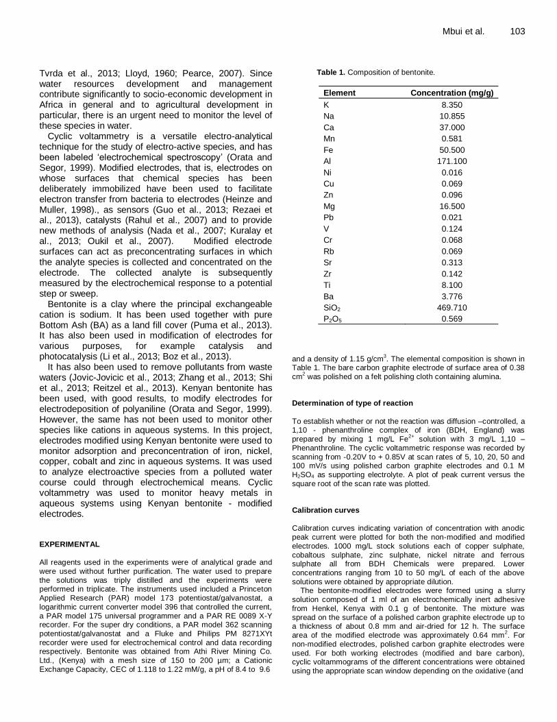
Table 1. Composition of bentonite.
Element Concentration (mg/g)
K 8.350
Na 10.855
Ca 37.000
Mn 0.581
Fe 50.500
Al 171.100
Ni 0.016
Cu 0.069
Zn 0.096
Mg 16.500
Pb 0.021
V 0.124
Cr 0.068
Rb 0.069
Sr 0.313
Zr 0.142
Ti 8.100
Ba 3.776
SiO2 469.710
P2O5 0.569
and a density of 1.15 g/cm
3. The elemental composition is shown in
Table 1. The bare carbon graphite electrode of surface area of 0.38 cm
2 was polished on a felt polishing cloth containing alumina.
Determination of type of reaction
To establish whether or not the reaction was diffusion –controlled, a 1,10 - phenanthroline complex of iron (BDH, England) was prepared by mixing 1 mg/L Fe
2+ solution with 3 mg/L 1,10 –
Phenanthroline. The cyclic voltammetric response was recorded by scanning from -0.20V to + 0.85V at scan rates of 5, 10, 20, 50 and 100 mV/s using polished carbon graphite electrodes and 0.1 M H2SO4 as supporting electrolyte. A plot of peak current versus the square root of the scan rate was plotted.
Calibration curves
Calibration curves indicating variation of concentration with anodic peak current were plotted for both the non-modified and modified electrodes. 1000 mg/L stock solutions each of copper sulphate, cobaltous sulphate, zinc sulphate, nickel nitrate and ferrous sulphate all from BDH Chemicals were prepared. Lower
concentrations ranging from 10 to 50 mg/L of each of the above solutions were obtained by appropriate dilution.
The bentonite-modified electrodes were formed using a slurry solution composed of 1 ml of an electrochemically inert adhesive from Henkel, Kenya with 0.1 g of bentonite. The mixture was spread on the surface of a polished carbon graphite electrode up to a thickness of about 0.8 mm and air-dried for 12 h. The surface area of the modified electrode was approximately 0.64 mm
2. For
non-modified electrodes, polished carbon graphite electrodes were
used. For both working electrodes (modified and bare carbon), cyclic voltammograms of the different concentrations were obtained using the appropriate scan window depending on the oxidative (and
104 Int. J. Phys. Sci.
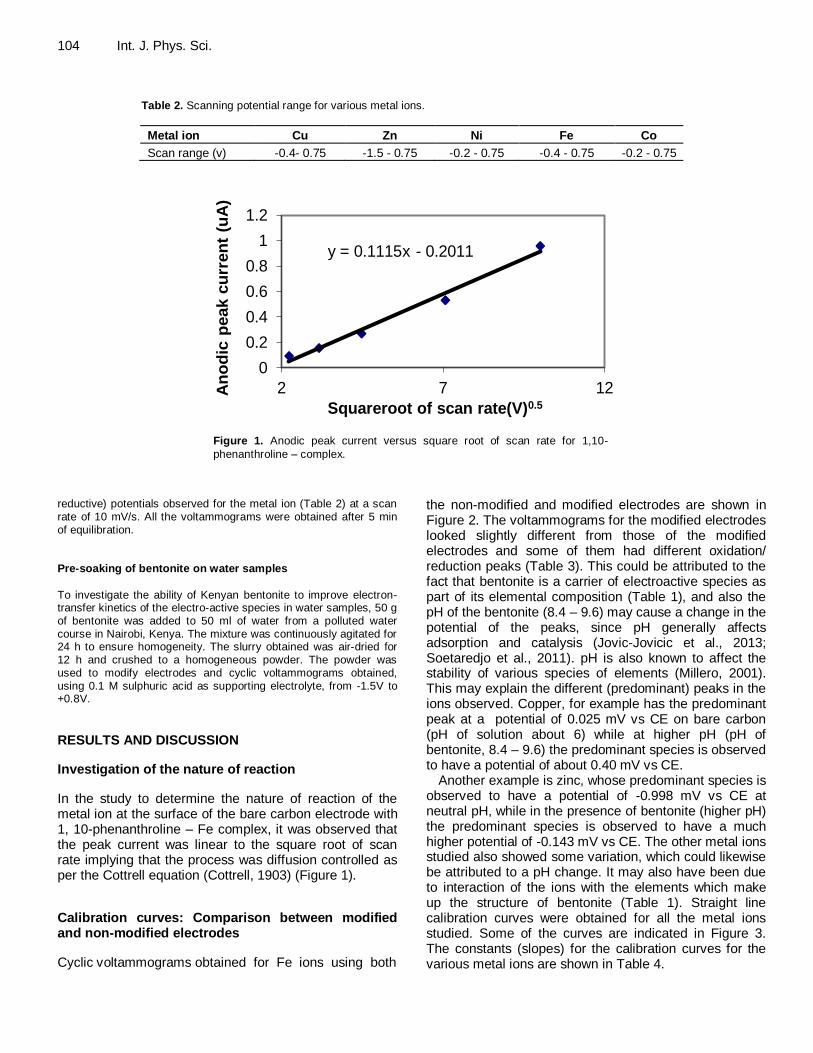
Table 2. Scanning potential range for various metal ions.
Metal ion Cu Zn Ni Fe Co
Scan range (v) -0.4- 0.75 -1.5 - 0.75 -0.2 - 0.75 -0.4 - 0.75 -0.2 - 0.75
y = 0.1115x - 0.2011
0
0.2
0.4
0.6
0.8
1
1.2
2 7 12An
od
ic p
eak c
urr
en
t (u
A)
Squareroot of scan rate(V)0.5
Figure 1. Anodic peak current versus square root of scan rate for 1,10-
phenanthroline – complex.
reductive) potentials observed for the metal ion (Table 2) at a scan rate of 10 mV/s. All the voltammograms were obtained after 5 min of equilibration. Pre-soaking of bentonite on water samples
To investigate the ability of Kenyan bentonite to improve electron-transfer kinetics of the electro-active species in water samples, 50 g
of bentonite was added to 50 ml of water from a polluted water course in Nairobi, Kenya. The mixture was continuously agitated for 24 h to ensure homogeneity. The slurry obtained was air-dried for 12 h and crushed to a homogeneous powder. The powder was used to modify electrodes and cyclic voltammograms obtained, using 0.1 M sulphuric acid as supporting electrolyte, from -1.5V to +0.8V.
RESULTS AND DISCUSSION
Investigation of the nature of reaction
In the study to determine the nature of reaction of the metal ion at the surface of the bare carbon electrode with 1, 10-phenanthroline – Fe complex, it was observed that the peak current was linear to the square root of scan rate implying that the process was diffusion controlled as per the Cottrell equation (Cottrell, 1903) (Figure 1).
Calibration curves: Comparison between modified and non-modified electrodes
Cyclic voltammograms obtained for Fe ions using both
the non-modified and modified electrodes are shown in Figure 2. The voltammograms for the modified electrodes looked slightly different from those of the modified electrodes and some of them had different oxidation/ reduction peaks (Table 3). This could be attributed to the fact that bentonite is a carrier of electroactive species as part of its elemental composition (Table 1), and also the pH of the bentonite (8.4 – 9.6) may cause a change in the potential of the peaks, since pH generally affects adsorption and catalysis (Jovic-Jovicic et al., 2013; Soetaredjo et al., 2011). pH is also known to affect the stability of various species of elements (Millero, 2001). This may explain the different (predominant) peaks in the ions observed. Copper, for example has the predominant peak at a potential of 0.025 mV vs CE on bare carbon (pH of solution about 6) while at higher pH (pH of bentonite, 8.4 – 9.6) the predominant species is observed to have a potential of about 0.40 mV vs CE.
Another example is zinc, whose predominant species is observed to have a potential of -0.998 mV vs CE at neutral pH, while in the presence of bentonite (higher pH) the predominant species is observed to have a much higher potential of -0.143 mV vs CE. The other metal ions studied also showed some variation, which could likewise be attributed to a pH change. It may also have been due to interaction of the ions with the elements which make up the structure of bentonite (Table 1). Straight line calibration curves were obtained for all the metal ions studied. Some of the curves are indicated in Figure 3. The constants (slopes) for the calibration curves for the various metal ions are shown in Table 4.

Mbui et al. 105
(i) (ii)
Figure 2. Cyclic voltammogram for Fe for unmodified (i) and modified (ii) electrodes.
Table 3. Anodic peak potentials of the metal ions Ep = of the non-modified electrode; Ep (CME) = of the modified
electrode.
Metal ion Cu Zn Ni Fe Co
Ep (V) (0.025±0.001)* -0.998±0.020 0.450±0.025 0.420±0.032 0.590±0.071
Ep(CME)(V) (0.462±0.010)* -0.143±0.035 0.464±0.040 0.414±0.089 0.386±0.009
* A number of peaks were observed. The largest peak was used to obtain the calibration curve.
(i) (ii)
y = 0.4022x - 35.909
0
20
40
60
80
70 170 270
An
od
ic p
ea
k c
urr
en
t (u
A)
Cu (II) Concentration (mg/L)
y = 2.8785x - 13.4
0
2
4
6
8
10
12
5 7 9
An
od
ic p
eak c
urr
en
t (u
A)
Copper concentration (mg/L)
Figure 3a. Peak current vs copper concentration for (i) unmodified and (ii) unmodified electrodes.
(i) (ii)
y = 0.124x - 3.1584
0
2
4
6
8
10
12
14
50 100 150Peak c
urr
en
t (u
A)
Zinc concentration (mg/L)
y = 2.9863x - 9.4014
4
6
8
10
12
14
16
18
4.5 6.5 8.5 10.5An
od
ic p
eak c
urr
en
t (u
A)
Zinc concentration (mg/L)
Figure 3b. Peak current versus zinc concentration for (i) unmodified and (ii) modified electrodes.
106 Int. J. Phys. Sci.
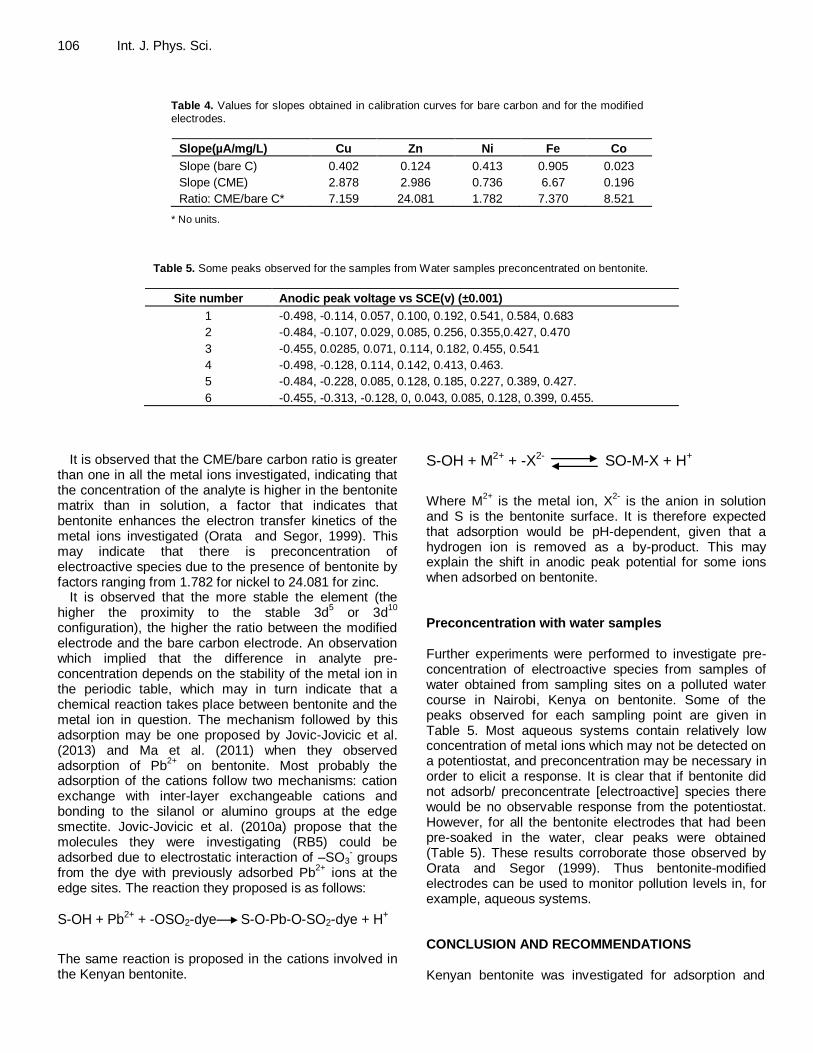
Table 4. Values for slopes obtained in calibration curves for bare carbon and for the modified electrodes.
Slope(µA/mg/L) Cu Zn Ni Fe Co
Slope (bare C) 0.402 0.124 0.413 0.905 0.023
Slope (CME) 2.878 2.986 0.736 6.67 0.196
Ratio: CME/bare C* 7.159 24.081 1.782 7.370 8.521
* No units.
Table 5. Some peaks observed for the samples from Water samples preconcentrated on bentonite.
Site number Anodic peak voltage vs SCE(v) (±0.001)
1 -0.498, -0.114, 0.057, 0.100, 0.192, 0.541, 0.584, 0.683
2 -0.484, -0.107, 0.029, 0.085, 0.256, 0.355,0.427, 0.470
3 -0.455, 0.0285, 0.071, 0.114, 0.182, 0.455, 0.541
4 -0.498, -0.128, 0.114, 0.142, 0.413, 0.463.
5 -0.484, -0.228, 0.085, 0.128, 0.185, 0.227, 0.389, 0.427.
6 -0.455, -0.313, -0.128, 0, 0.043, 0.085, 0.128, 0.399, 0.455.
It is observed that the CME/bare carbon ratio is greater than one in all the metal ions investigated, indicating that the concentration of the analyte is higher in the bentonite matrix than in solution, a factor that indicates that bentonite enhances the electron transfer kinetics of the metal ions investigated (Orata and Segor, 1999). This may indicate that there is preconcentration of electroactive species due to the presence of bentonite by factors ranging from 1.782 for nickel to 24.081 for zinc.
It is observed that the more stable the element (the higher the proximity to the stable 3d
5 or 3d
10
configuration), the higher the ratio between the modified electrode and the bare carbon electrode. An observation which implied that the difference in analyte pre-concentration depends on the stability of the metal ion in the periodic table, which may in turn indicate that a chemical reaction takes place between bentonite and the metal ion in question. The mechanism followed by this adsorption may be one proposed by Jovic-Jovicic et al. (2013) and Ma et al. (2011) when they observed adsorption of Pb
2+ on bentonite. Most probably the
adsorption of the cations follow two mechanisms: cation exchange with inter-layer exchangeable cations and bonding to the silanol or alumino groups at the edge smectite. Jovic-Jovicic et al. (2010a) propose that the molecules they were investigating (RB5) could be adsorbed due to electrostatic interaction of –SO3
- groups
from the dye with previously adsorbed Pb2+
ions at the edge sites. The reaction they proposed is as follows:
S-OH + Pb2+ + -OSO2-dye S-O-Pb-O-SO2-dye + H+
The same reaction is proposed in the cations involved in the Kenyan bentonite.
S-OH + M2+ + -X2- SO-M-X + H+
Where M
2+ is the metal ion, X
2- is the anion in solution
and S is the bentonite surface. It is therefore expected that adsorption would be pH-dependent, given that a hydrogen ion is removed as a by-product. This may explain the shift in anodic peak potential for some ions when adsorbed on bentonite. Preconcentration with water samples Further experiments were performed to investigate pre-concentration of electroactive species from samples of water obtained from sampling sites on a polluted water course in Nairobi, Kenya on bentonite. Some of the peaks observed for each sampling point are given in Table 5. Most aqueous systems contain relatively low concentration of metal ions which may not be detected on a potentiostat, and preconcentration may be necessary in order to elicit a response. It is clear that if bentonite did not adsorb/ preconcentrate [electroactive] species there would be no observable response from the potentiostat. However, for all the bentonite electrodes that had been pre-soaked in the water, clear peaks were obtained (Table 5). These results corroborate those observed by Orata and Segor (1999). Thus bentonite-modified electrodes can be used to monitor pollution levels in, for example, aqueous systems. CONCLUSION AND RECOMMENDATIONS Kenyan bentonite was investigated for adsorption and

preconcentration of metal ions. Straight line calibration curves were obtained with bentonite-modified electrodes with slopes of between 0.196 and 2.986 µA/mg/L. The slopes of the curves of modified electrodes were higher than those of non-modified electrodes by a factor of between 1.7 and 24 which means that bentonite adsorbed and preconcentrated the metal ions. It was also observed that the magnitude of the ratio depended on the proximity of the ion being investigated to the stable 3d configuration (either filled or half-filled 3d orbitals). This may mean that chemical rather than physical adsorption took place. When electrodes were modified with bentonite that had been soaked with water samples from a polluted water course, the reponse indicated that the electroactive species in the water could be detected on a potentiostat. Thus Kenyan bentonite can be used in analysis of species in aqueous solution through preconcentrating the species on the bentonite. Spiking can be used to identify the species observed on preconcentration on water samples on bentonite. It is also recommended that other methods (eg. computational speciation programs) be used to compare the species observed electrochemically with those suggested by such programs.
ACKNOWLEDGEMENT
Author would like to acknowledge The German Academic Exchange Service (DAAD) for providing funds to carry out the project and also acknowledge the Eric Abraham Academic Visitorship (EAAV) for funds at the University of Cape Town.
Conflict of Interest
The author(s) have not declared any conflict of interests.
REFERENCES
Boz N, Degirmenbasi NK, Dihan M (2013). Transesterification reaction
of canola oil to biodiesel using calcium bentonite functionalized with K compounds. Appl. Catalysis B-Environ. 138:236–242. http://dx.doi.org/10.1016/j.apcatb.2013.02.043
Cottrell FG (1903). Der Reststrom bein galvanischer Polarisation betrachtet als ein Diffusions problem. Inaugural Dissertation, University of Leipsig. Also published in Zeit. Phys. Chem. 42:385-
431. Elbetieba A, Al-Hammod MH (1997). Long term Exposure of Male and
Female Mice to trivalent and hexavalent chromium compounds:
Effect of Fertility. Toxicology. 116:19–47. Guo K, Chen X, Freguia S, Donose B, Dan C (2013). Spontaneous
modification of carbon surfaces with neutral red from its diazonium
salts for bioelectrochemical systems. Biosensors and bioelectronics. 47:184–189. http://dx.doi.org/10.1016/j.bios.2013.02.051 PMid:23578972
Heinze J, Muller R (1998). Direct Electrochemical Detection of C60 in Solution by steady-state voltammetry at microelectrodes. J.
Mbui et al. 107
Electrochem. Soc. 145:1227–1232. http://dx.doi.org/10.1149/1.1838443
Jovic-Jovicic N, Milutinovic-Nikolic A, Bankovic P, Mojovic Z, Zunic M,
Grzetic I, Jovanovic D (2010a). Organo-inorganic Bentonite for simultaneous adsorption of acid orange 10 and lead ions. Appl. Clay Sci. 47(3-4):452–456. http://dx.doi.org/10.1016/j.clay.2009.11.005
Jovic–Jovivic NP, Milutinovic-Nikolic AD, Zunic MJ, Mojovic ZD, Bankovic PT, Grzetic IA, Jovanovic DM (2013). Synergic Adsorption of Pb2+ and reactive dye – RB5 on organo-modified bentonites. J.
Contaminant Hydrol. 50:1–11. http://dx.doi.org/10.1016/j.jconhyd.2013.03.004 PMid:23624568
Kuralay F, Erkut Y, Lokman U, Adil D (2013). Cibacron Blue F3GA
modified disposable pencil graphite electrode for the investigation of affinity binding to bovine serum albumin. Colloids surfaces. B: biointerfaces. 110:270–274.
http://dx.doi.org/10.1016/j.colsurfb.2013.04.024 PMid:23732804 Li YM, Zhang Y, Li J, Sheng G, Zheng X (2013). Enhanced reduction of
chlorophenols by nanoscale zerovalent iron supported on bentonite.
Chemosphere. 92(4). http://dx.doi.org/10.1016/j.chemosphere.2013.01.030
Lloyd R (1960). Great Britain department of scientific and industrial
research. Water Pollution Res. P. 83. Ma J, Cui B, Dai J, Li D (2011). Mechanism of adsorption of anionic dye
from aqueous solution onto organo bentonite. J. Hazardous mater.
86(2-3):1758–1765. http://dx.doi.org/10.1016/j.jhazmat.2010.12.073 PMid:21227582
Millero F (2001). Speciation of metals in natural waters. Geochemical
Translations. 8. (article) http://dx.doi.org/10.1186/1467-4866-2-57 Nada FA, Soher AD, Sayed EK, Gala A (2007). Effect of Surfactants on
the voltammetric response and determination of an antihypersentive
drug. J. talanta 72(4):1438–1445. Normandin L (2004). Manganese distribution in the brain and
neurobehavioral changes following inhalation exposure of rats to
three chemical forms of manganese. Neurotoxicology. 25(3):433-441. http://dx.doi.org/10.1016/j.neuro.2003.10.001 PMid:15019306
Orata D, Segor F (1999) Bentonite (Clay montmorillonite) as a template
for electrosynthesis of thyroxine, Catalysis Lett. 58:157-162. http://dx.doi.org/10.1023/A:1019038219556
Oukil D, Makhloufi L, Saidani B (2007). Preparation of polypyrolle films
containing ferrocyanide ions deposited onto thermally pretreated and untreated iron substrate. Application in the electroanalytical determination of ascorbic acid. J. Sensors Actuators B: Chemical.
123(2)1083–1089. http://dx.doi.org/10.1016/j.snb.2006.11.014 Pearce JMS (2007). "Burton's line in lead poisoning". European neurol.
57(2):118–119. http://dx.doi.org/10.1159/000098100 PMid:17179719
Puma S, Marchese F, Dominijanni A, Manassero M (2013). Reuse of MSWI bottom Ash mixed with natural sodium bentonite as landfill cover material. Waste Manage. Res. 31(6):577–584. http://dx.doi.org/10.1177/0734242X13477722 PMid:23478909
Rahul MK, Purvi BD, Ashwini KS (2007). Behaviour of riboflavin on plain carbon paste and aza macrocycles based chemically modified electrodes. J. Sensors Actuators B: Chemical. 124(1):90–98.
http://dx.doi.org/10.1016/j.snb.2006.12.004 Reitzel K, Andersen FO, Egemose S, Jensen HS (2013). Phosphate
adsorption by Lanthanum modified bentonite clay in Fresh and
brakish water. Water Res. 47(8):2787–2796. http://dx.doi.org/10.1016/j.watres.2013.02.051 PMid:23521977
Rezaei B, Elaheh H, Ensafi AA (2013). Stainless Steel modified with an
aminosilane layer and gold nanoparticles as a novel disposable substrate for impedimetric immunosensors. Biosensors and Electronics. 58:61–66.
Shi LN, Zhou Y, Chen Z, Megharey M, Naidu R (2013). Simultaneous adsorption and degradation of Zn2+ and Cu2+ from Waste waters using nanoscale zero—valent iron impregnated with clays. Environ.
Sci. Pollution Res. 20(6):3639–3648. http://dx.doi.org/10.1007/s11356-012-1272-7 PMid:23114838
Soetaredjo FE, Ayucitra A, Ismadji S, Mankar AL (2011). KOH/bentonite
catalysts for transesterification of palm oil to biodiesel. 53:341–346. Tvrda E, Zuzana K, Jana L, Monika S, Zofia G, Agniezka G, Csaba S,
Peter M, Norbert L (2013). The impact of lead and cadmium on
selected motility, proxidant and antioxidant parameters of bovine seminal plasma and spermatozoa. J. Environ. Sci. Health part A –

108 Int. J. Phys. Sci.
Toxic/Hazardous Substances Environ. Eng. 48(10):1292–1300. UNEP/GEMS (1991). Fresh water Pollution. UNEP/GEMS
Environmental Library No. 6. UNEP.
Zhang YJ, Liu LC, Chen DP (2013). Synthesis of Cd/S bentonite nanocomposite powders for H – 2 production by photocatalytic decomposition of water. Powder Technol. 241:7–11.
http://dx.doi.org/10.1016/j.powtec.2013.02.031

International Journal of Physical Sciences
Related Journals Published by Academic Journals
■African Journal of Pure and Applied Chemistry■Journal of Internet and Information Systems■Journal of Geology and Mining Research■Journal of Oceanography and Marine Science■Journal of Environmental Chemistry and Ecotoxicology■Journal of Petroleum Technology and Alternative Fuels