International Journal of Heat and Mass Transfer 73 (2014) 716–730

Contents lists available at ScienceDirect

International Journal of Heat and Mass Transfer

journal homepage: www.elsevier .com/locate / i jhmt

Statistical analysis of measured and computed thickness and interfacialtemperature of free-falling turbulent liquid films

http://dx.doi.org/10.1016/j.ijheatmasstransfer.2014.02.0540017-9310/� 2014 Elsevier Ltd. All rights reserved.

⇑ Corresponding author. Tel.: +1 765 494 5705; fax: +1 765 494 0539.E-mail address: mudawar@ecn.purdue.edu (I. Mudawar).URL: https://engineering.purdue.edu/BTPFL (I. Mudawar).

Nikhin Mascarenhas, Issam Mudawar ⇑Purdue University Boiling and Two-Phase Flow Laboratory (PU-BTPFL), School of Mechanical Engineering, 585 Purdue Mall, West Lafayette, IN 47907, USA

a r t i c l e i n f o a b s t r a c t

Article history:Received 10 October 2013Received in revised form 18 February 2014Accepted 19 February 2014Available online 19 March 2014

Keywords:Falling filmsWavinessTurbulenceProbability densityCovarianceSpectral analysis

This study examines the evolution of film thickness and interfacial temperature in turbulent, free-fallingwater films that are subjected to sensible heating. Measured temporal records of film thickness and inter-facial temperature are subjected to thorough statistical analysis to understand the influence of interfacialwaves on the distribution, periodicity and interdependence of these two parameters. A computationalmodel of the film is constructed and its predictions subjected to similar statistical analysis. The statisticaltools employed in this study include probability density, auto-covariance, cross-covariance, auto-spec-trum and cross-spectrum. Probability density of film thickness shows an increase in substrate thicknessand amplitude with increasing Reynolds number, while auto-covariance of thickness captures dominantfrequencies corresponding to the large waves. Cross-covariance of film thickness and interfacial temper-ature difference captures a clear phase shift between the two parameters, with the temperature reachinga maximum in the relatively thin film region between the substrate and wave peak. Statistical results forboth parameters exhibit clear dependence on axial location in the thermal entrance region, and point tofully developed wave structure downstream. The statistical results based on computed film thickness andinterfacial temperature difference agree well with the results based on the measured, which demon-strates the effectiveness of the adopted computational tools at predicting the complex transport phenom-ena associated with wavy liquid–vapor interfaces.

� 2014 Elsevier Ltd. All rights reserved.

1. Introduction

Gravity-driven two-phase systems are very popular in manyindustries because of their ability to achieve very high heat transfercoefficients while avoiding the penalty of high pressure drop.These systems include pool boiling thermosyphons [1,2] andpumpless gravity driven loops [3,4].

Free-falling liquid films are found in another type of gravity-driven systems that feature high heat transfer coefficients, whichinclude condensers, evaporators, spray-type refrigerators, distilla-tion columns, chemical reactors, and nuclear reactors. The attrac-tive thermal attributes of free-falling liquid films are realized byminimizing conduction resistance for thin laminar films and capi-talizing upon both turbulent fluctuations (for high film flow rates)and added mixing provided by interfacial waves. But despite manydecades of efforts to model the transport characteristics of free-falling films, uncertainty remains concerning the dampening ofturbulent eddies at the film interface due to surface tension, tran-

sition from laminar to turbulent flow, and, most importantly, theinfluence of interfacial waves.

1.1. Interfacial characteristics of falling films

Liquid films found in thermal devices are typically thin, exhibitturbulent flow and rely on gravity to achieve fluid motion. Theafore-mentioned attributes of films are highly complicated by theprevalence of interfacial waves spanning a broad range of speedsand length scales. At a first glance, time records appear to showlarge waves that have a profound influence on temperaturedistribution across the film as shown in Fig. 1(a) and (b). However,there are appreciable variations in shape, speed and frequency ofoccurrence of these large waves, in addition to seemingly highlystochastic smaller waves, some of which are superimposed onthe large waves.

In a recent study by the authors of the present study [7], timerecords of film thickness were inspected and repeatable wave pat-terns identified for different film Reynolds numbers in pursuit oftime-averaged values for film thickness, heat transfer coefficient,and both temperature and eddy diffusivity profiles across the film.

Nomenclature

C cross-covarianceCl turbulence model constantDH hydraulic diameterf frequencyg gravitational accelerationk thermal conductivity; turbulent kinetic energyL total number of lags in auto-spectra and cross-spectraN number of discrete data pointsn number of samples in subset of data recordP pressure; probabilityp probability densityPr Prandtl numberPrt turbulent Prandtl numberq00w wall heat fluxr radial coordinateR auto-covarianceRe Reynolds number, Re = 4C/lS auto-spectrumsij fluctuating component of strain rate tensorT temperaturet timeu velocityU inlet streamwise velocityur r-direction velocity componentux x-direction velocity componentV inlet normal velocityW cross-spectrumw window function in auto-spectra and cross-spectra

x axial coordinatey coordinate perpendicular to the wall

Greek Symbolsa thermal diffusivityU mass flow rate per unit film widthd film thicknessD difference between adjacent covariance valuese dissipation rate of turbulent kinetic energyl dynamic viscositym kinematic viscosityq densityr2 variances time lag

Subscriptsi film interfacein inletmin minimums solidt turbulentw wall

Superscripts� average+ non-dimensionalized0 fluctuating component

N. Mascarenhas, I. Mudawar / International Journal of Heat and Mass Transfer 73 (2014) 716–730 717

A closer examination of the time records for large waves in a sub-sequent study [5] revealed (i) both periodic and non-periodic inter-facial features, and (ii) a strong correlation between film thicknessand liquid temperature with an identifiable phase shift as shown inFig. 1(a). These findings clearly point to the need to further explorethe interfacial behavior of films using statistical tools. Such toolscan be quite effective at identifying any salient and/or repeatableaspects of interfacial behavior.

1.2. Statistical description of interfacial behavior

Phillips [8] studied the structure of waves generated by windblowing over a large area of the ocean for a long duration anddetermined statistics for small-scale components of the wave. Astatistical equilibrium range in the wave height spectrum wasidentified and subjected to dimensional analysis to assess theinfluence of gravity and wavelength of small waves on the magni-tude of the spectrum. Telles and Dukler [9] inspected the interfa-cial structure of a liquid film that is shear-driven by a gas flowby tracking film thickness fluctuations using electrical conductivitymethods. A significant portion of the film was comprised of largestable liquid humps – large waves - marred by smaller waves thatlost their identity over small distances. Statistical methods wereimplemented to calculate wave speed, separation distance be-tween humps, amplitude, frequency, and wave shape, for Reynoldsnumbers as high as Re = 60,000. Chu and Dukler [10] further re-fined these methods and compared them to predictions of a theorythey developed for mean substrate thickness and substrate flowrate. This enabled them to demonstrate the importance of the sub-strate in controlling the film’s transport processes. Using probabil-ity density distribution of film thickness for high Re, Chu andDukler [11] showed that the film possessed bimodal characteristics

consisting of large and small waves. They also concluded that largewaves dominate transport characteristics in the film, while smallwaves control transport characteristics in the gas.

Use of statistical methods to decipher salient flow characteris-tics is well recognized in two-phase research. Aside from temporalfluctuations in key flow parameters, two-phase flow measure-ments are complicated by intermittence between the two phases.Jones and Delhaye [12] reviewed the experimental techniques usedto measure two-phase flow parameters, and emphasized theimportance of employing statistical tools to tackle the complextemporal characteristics of the measured parameters. Takahamaand Kato [13] used needle contact and electrical capacitanceprobes to measure the thickness of falling films, and showed thatinterfacial waves can be effectively characterized over broad flowrate ranges using normal, logarithmic normal and gamma proba-bility distributions of film thickness. Nencini and Andreussi [14]employed statistical methods to analyze experimental data forannular two-phase downflow. Statistical analysis of the largewaves and substrate yielded flow rates that agreed well with theactual flow rates. Karapantsios et al. [15] performed a comprehen-sive experimental and statistical study of falling films. Film thick-ness data measured for Re = 509–13,090 with a wire conductancetechnique were subjected to statistical analysis using probabilitydensity, spectral density, skewness and kurtosis. Lyu and Mudawar[6] performed experiments to investigate the relationship betweenfilm thickness and water film temperature for various film Rey-nolds numbers. Using statistical tools, the relationship betweenthe two variables was shown to be stronger at high compared tolow heat fluxes. A cross-spectrum analysis showed a distinct bandof dominant frequencies in the relationship between the two vari-ables. Ambrosini et al. [16] used capacitance probes to measure thethickness of water films falling freely down vertical and inclined

Fig. 1. Measurements at x = 278 mm for free-falling water film subjected to sensible heating with Re = 5700, Pr = 5.86 and q00w = 50,000 W/m2: (a) temporal records of liquidtemperature and film thickness (adapted from [5]), and (b) three-dimensional plot of liquid temperature variations with distance from the wall and time (adapted from [6]).

718 N. Mascarenhas, I. Mudawar / International Journal of Heat and Mass Transfer 73 (2014) 716–730

surfaces for a range of Reynolds numbers encompassing both tran-sition and turbulent flows. They collected film thickness time ser-ies and used statistical tools to determine mean, minimum andmaximum film thickness and wave velocity, and presented powerspectra as functions of film flow rate, plate inclination and filmtemperature.

The present study employs statistical tools to explore the trans-port behavior of turbulent free-falling liquid films that are sub-jected to sensible heating. Given the aforementioned importanceof interfacial waves on the film’s mass, momentum and heat trans-fer characteristics, these statistical tools are used to investigatetemporal records of both film thickness and interfacial tempera-ture, as well as the relationship between the interfacial wave char-acteristics and those of liquid temperature. The same statisticaltools are also applied to temporal records of the film computedusing FLUENT. The statistical results based on the measured andcomputed records are used to validate the effectiveness of compu-tational methods at capturing the correct interfacial profile andinfluence of waves on the film’s transport characteristics. A varietyof statistical tools are employed for this purpose. Probability den-sity is used to capture dominant ranges of film thickness and liquidtemperature. Auto-covariance and cross-covariance are employedto describe the interdependence between waves and liquid tem-perature, and auto-spectra and cross-spectra to segregate wavefrequencies in pursuit of identifying large and small waves.

2. Experimental methods

The data utilized in this study were obtained from measure-ments made using the Purdue University Boiling and Two-PhaseFlow Laboratory (PU-BTPFL) falling film facility. This facility hasyielded data for liquid films subjected to sensible heating [5–7,17–19], evaporation [20] and boiling [21]. Two distinct sets offilm thickness instrumentation tools are used in this facility. Thefirst, which is described in [7], provide time-averaged measure-ments of wall and mean film temperatures. The second, whichare used to measure simultaneous instantaneous film thicknessand temperature profile, are detailed in [5] and described briefly

below, are employed in measuring the data discussed in the pres-ent study. The data for turbulent free-falling water films subjectedto sensible heating are examined with the aid of several statisticaltools and compared to computational predictions.

Fig. 2(a) shows the central component of the falling film facility,a test chamber where the falling film is generated on the outsidewall of a vertical 25.4-mm diameter test section. The test sectionis comprised of three portions. The film is formed by passing waterthrough the porous wall of a 300-mm long polyethylene tube. Thefilm is formed gradually on the outside wall of the porous tube,which is followed by a 757-mm long adiabatic G-10 plastic tube,over which the film is allowed to develop hydrodynamically. Thefilm is heated along the lower 781-mm long stainless steel tube,which is electrically heated by a d.c. power source to supply a uni-form wall heat flux to the film.

As shown in Fig. 2(a), 17 pairs of type-T thermocouples are in-serted along the length of the stainless steel tube to measure theinside wall temperature. Axial distance between thermocouplesis smaller near the top of the stainless steel tube compared todownstream in order to capture thermal entrance effects. At eachaxial location, the thermocouples pairs at each axial location areplaced diametrically opposite to one another to capture and correctany asymmetry resulting from vertical misalignment. Fig. 2(b) de-tails the construction of the wall thermocouples. Each thermocou-ple bead is embedded in a small mass of thermally conductingboron nitride epoxy that is deposited into the head of a 6–32 nylonsocket head cap screw. The outer surface of the boron nitride iscarefully machined to match the curvature of the inner wall ofthe stainless steel tube. The screw is inserted radially into an innerthermally insulating tube made from Delrin plastic. A small springmaintains positive pressure between the boron nitride epoxy andstainless steel tube.

Fig. 2(c) shows the flow loop that supplies deionized water tothe test chamber at carefully regulated flow rate, temperatureand pressure. The water is deaerated in a stainless steel reservoirfitted with immersion heaters and a reflux condenser before beingcharging into the flow loop.

Instantaneous film thickness, film temperature profile and wavevelocity measurements are made with the aid of several delicate

Fig. 2. (a) Cut-away view of test chamber. (b) Cross-sectional view of inner thermocouples. (c) Schematic diagram of flow loop.

N. Mascarenhas, I. Mudawar / International Journal of Heat and Mass Transfer 73 (2014) 716–730 719

probes that are mounted on an assembly block as shown inFig. 3(a). The block itself is centered around the stainless steel tubeby means of six alignment screws that are situated downstream ofthe probes to preclude any influence to the film measurements.Axial movement of the block is aided by a vertical guide rail, whichis connected to two external micrometer translation stages thatcontrol the assembly block’s horizontal position. The probes con-sist of a thermocouple array, thickness probe and a thickness cali-bration probe, all mounted in the same horizontal plane. A secondthickness probe used for wave velocity measurements is situated29.7 mm downstream with a 41� azimuthal offset to avoid theinfluence of wakes created by the upstream probes.

The thermocouple array is further detailed in Fig. 3(b), whichshows twelve type-E 0.0762-mm diameter thermocouple beadsmade from 0.0508 mm wire that are distributed over a 5-mm spanfrom the heated wall, supported on a G-10 fiberglass plastic knife-edge. Thermocouple locations are denser near the stainless steelwall to capture the near-wall thermal boundary layer. A protrusionon the downstream edge of the plastic knife–edge plate preventsthe instrumented portion from making direct contact with thewall. The maximum standard deviation of temperature fluctuationfor each thermocouple is 0.17 �C, which is dictated by the highspeed data acquisition system. The thermocouples are calibratedin a constant temperature bath at several temperatures. This isachieved by filling the lower portion of the test chamber withwater with the probe assembly block completely submerged. Elec-trical current is then supplied across the stainless steel tube to the

same heat flux levels applied during the subsequent falling filmexperiments to calibrate the thermocouples for offset resultingfrom the d.c. current. The calibration procedure is repeated severaltimes after using each batch of deionized water in the falling filmconfiguration to maintain thermocouple offset below 0.2 �C.

The primary thickness probe used for instantaneous film thick-ness measurement is based on the principle of hot-wire anemom-etry. Shown in Fig. 3(c), this probe is made from 0.0254-mmdiameter platinum-10% rhodium wire that is extended across theliquid–vapor interface. A constant d.c. current is supplied throughthe wire, and film thickness inferred from variations in the probe’svoltage drop. This technique takes into account the large ratio ofheat transfer coefficient along the portion of probe wire submergedin liquid compared to that in vapor, as well as the relationship be-tween electrical resistance and temperature. Once calibrated, pas-sage of a constant current through the probe wire yields a voltagedrop that is a function of the length of wire submerged in liquidalone.

Extensive calibration is required to ensure accurate film thick-ness measurement. This includes first submerging the probe verti-cally downward in a small test cell containing a stagnant layer ofwater to generate the linear dependence of voltage drop on waterlayer thickness. This is followed by in situ calibration that is per-formed prior to each test at heating conditions identical to thoseof the test itself using the calibration probe shown in Fig. 3(c).The measurement resolution and response time of the thicknessprobe are 0.05 mm and 0.14 ms, respectively [19].

Fig. 3. Construction of (a) probe assembly, (b) thermocouple knife-edge, and (c) thickness probe and thickness calibration probe.

720 N. Mascarenhas, I. Mudawar / International Journal of Heat and Mass Transfer 73 (2014) 716–730

N. Mascarenhas, I. Mudawar / International Journal of Heat and Mass Transfer 73 (2014) 716–730 721

Instantaneous temperature measurements across the film aremade simultaneously with the film thickness measurements overa sampling period of 1 s at a frequency of 500 Hz. The temperaturedata are low-pass filtered using a fourth order 0.1 dB Chebyshevdigital filter code written by Walraven [22].

3. Numerical methods

Falling film tests performed using the experimental methodsdescribed in the previous section are simulated using the FLUENTAnalysis System in the Toolbox of ANSYS Workbench 14.0.0 [23].In recent years, the flow modeling capability of FLUENT has beenexpanded by researchers to enhance turbulence prediction and in-clude two-phase flows and phase change [24–30]. In the presentstudy, the Project Schematic of Workbench in ANSYS FLUENT14.5 is utilized to construct and mesh the thermally active flow do-main, as well as to generate and extract instantaneous data thatcan be compared to the measurements.

Fig. 4 shows the computational domain, a 2-dimensional axi-symmetric system, which is justified by the small film thickness.The key components of the domain are the inlet reservoir, porousfilm distributor, and 1835-mm long annulus formed between theouter wall of the 25.4-mm test section and inner walls of the testchamber. An annulus thickness is assigned to yield a flow areaequal to the actual flow area between the test section and testchamber walls.

The computation utilizes conservation equations for unsteady,turbulent and incompressible flow with constant properties. Usingthe Reynolds’ decomposition [31], ux ¼ ux þ u0x, ur ¼ ur þ u0r andT ¼ T þ T 0. The corresponding equations for time-averaged conti-nuity, axial and radial momentum, and energy, respectively, areexpressed for the fluid region as [32]

@ux

@xþ 1

r@ðrurÞ@r

¼ 0; ð1Þ

q@ux

@tþ ux

@ux

@xþ ur

@ux

@r

� �¼ � @P

@xþ 2

@

@xl @ux

@x

� �þ 1

r

� @

@rrl @ux

@rþ @ur

@x

� �� �

� q@u02x@xþ @ðu

0xu0rÞ@r

þ u0xu0rr

� �þ qg; ð2Þ

q@ur

@tþ ux

@ur

@xþ ur

@ur

@r

� �¼ � @P

@rþ @

@xl @ux

@rþ @ur

@x

� �� �

þ 21r@

@rrl @ur

@r

� �� 2lur

r2

� q@ðu0xu0rÞ@x

þ @u02r@rþ u02r

r

� �; ð3Þ

and

@T@tþux

@T@xþur

@T@r¼ @

@xa@T@x�hu0xT 0i

!þ1

r@

@rar@T@r� rhu0rT

0i !

: ð4Þ

The standard two-equation k � e turbulent model, as prescribedin the ANSYS Guide [23], is used to provide closure to the unre-solved Reynolds stress terms. The fluctuating terms are expressedin terms of the gradients of the mean quantities in accordance withthe eddy viscosity hypothesis, where the eddy viscosity, lt, is ex-pressed as

lt ¼Clqk2

e: ð5Þ

The kinetic energy and dissipation energy equations are given,respectively, by

2r:l ~rsij

D E¼ @

@xl @k

@xþ @hu

02x i

@xþ 1

r@rhu0xu0ri

@r

� �

þ 1r@

@rlr

@k@rþ @hu

0xu0ri@x

þ 1r@rhu02r i@r

� �ð6Þ

and

e ¼ 2q

lhhsijsijii; ð7Þ

where

sij ¼@u0r@xþ @u0x@r

: ð8Þ

The boundary conditions are specified as follows. Velocity andliquid temperature in the reservoir inlet are assumed uniformand adjusted according to values of the film’s Reynolds and Prandtlnumber: U = mRe/DH, V = 0, and T = Tin(Pr) for x = �1060 mm and�12.7 mm 6 r 6 �6.6 mm. The outlet condition at the bottom ofthe domain is assumed to be uniform pressure equal to atmo-sphere to conform to experimental conditions. Also to conform tothe data, a constant heat flux is applied along the lower stainlesssteel portion of the test section that results in a temperature riseequal to that produced experimentally across the thermally-devel-oping span of the film, �ks@T=@r ¼ q00w for 0 6 x 6 781 mm.

The interfacial treatment considers the influences of surfacetension and molecular viscosity, and neglects the vapor shear atthe film interface. The tangential and normal force balance equa-tions at the film surface are always satisfied. The curvature termsin these equations are calculated in each cell by FLUENT from thevolume fraction gradients, as per the continuum surface forcemodel proposed by Brackbill et al. [33]. These tangential and nor-mal forces perturb the interface, and instabilities are amplified bythe turbulent nature of the flow.

At the wall, surface tension effects are considered by prescrib-ing wall adhesion in terms of contact angle. The viscosity-influenced near-wall region is completely resolved all the way tothe viscous sublayer, and both e and turbulent viscosity are speci-fied. This region is further subdivided into a viscosity-influencedregion and a fully turbulent region, whose separation is deter-mined by a wall-distance-based turbulent Reynolds number. Inthe fully turbulent region, the k � e model is employed to defineturbulent viscosity, while the one-equation model of Wolfstein[34] is applied in the viscosity-influenced near-wall region. In thelatter model, the momentum and k equations are retained, andthe length scale for turbulent viscosity is derived according to Chenand Patel [35]. Jongen [36] derived a technique for smoothly blend-ing this two-layer definition for turbulent viscosity with the highReynolds number definition from the outer region. FLUENT utilizesthis two-layer model with a modified single function formulationof the law of the wall for the entire wall region by blending laminarand turbulent law of the wall relations as per Kader [37]. This for-mulation guarantees correct asymptotic behavior for large andsmall values of y+ and reasonable representation of velocity pro-files where y+ falls inside the buffer region. This method involvesmodification of the fully turbulent relation and takes into accountother effects such as pressure gradients or variable properties. Thewalls are governed by continuities of both temperature and heatflux, and the wall heat flux is applied by conduction normal tothe fluid body.

Two-phase treatment follows the Volume of Fluid (VOF) model[38]. From an examination of turbulence models presented in [7],and following numerical turbulence studies by Kays [39], aconstant turbulent Prandtl number value of Prt = 1 is used. Theconstant Cl in Eq. (5) is set equal to 0.09. The porous film distrib-utor has a porosity of 0.002 and a viscous resistance of3.846 � 07 m�2. In order to conserve computation time, the

722 N. Mascarenhas, I. Mudawar / International Journal of Heat and Mass Transfer 73 (2014) 716–730

fractional step version of the non-iterative time advancement(NITA) scheme is used with first-order implicit discretization atevery time-step [40,41] to obtain pressure–velocity coupling. Gra-dient generation during spatial discretization is accomplishedusing the least-squares cell-based scheme [42], while PRESTO,QUICK, Geo-reconstruct and first-order upwind schemes [43] areused for pressure, momentum, volume fraction and turbulent ki-netic energy resolution, respectively.

The grid system consists of 401,426 nodes and 397,111 cells,which is arrived at after careful assessment in pursuit of optimumdegree of mesh refinement. This process involves evaluating theinfluence of mesh size on computational effort and quality of re-sults. The grid system used is non-uniform, with a larger numberof grid points near the wall, film interface, porous zone and heatedportion of the test section to achieve superior accuracy in resolvingkey flow parameters. Although the bulk flow region of the fallingfilm is modeled using a mesh size estimated to capture turbulencequite well, an order of magnitude refinement in the mesh isadopted beginning well outside the narrow viscous layer at theinterface to ensure high resolution in capturing turbulence at theinterface. It is important to note that the transition in refinementis gradual to avoid influencing the flow.

4. Statistical results

4.1. Statistical approach

The method adopted in this study to explore the statisticalparameters of the falling liquid film consists of (i) applying statis-tical functions directly to the measured temporal records of bothfilm thickness and liquid temperature, (ii) applying identical statis-tical functions to the computed thickness and temperature, and(iii) comparing statistical results from the measured and computedtime records as a means of validating the effectiveness of compu-

rx

q”

760(AdiabaticSection)

781(HeatedSection)

300(PorousSection) 12.7

6.1

All dimensions in mm

Inlet

Outlet

28.6

w

Fig. 4. Computational domain.

tational methods at capturing the interfacial profile and influenceof waves on liquid temperature for free-falling turbulent liquidfilms.

The statistical functions are applied to temporal records similarto those shown in Fig. 1(a) and (b). These records are treated astime series and examined with the aid of statistical tools. The vari-ables that are examined here are assumed stationary (i.e., theirmean and variance do not change over time) in order to apply timeinvariant statistical functions. It is also assumed that the variablesare ergodic (i.e., their average value over a long time period can beequated to the average of values obtained at different times). Pre-sented below are probability density, covariance and spectral plotsof both film thickness and interfacial temperature.

4.2. Probability density and variance results

Probability density of a variable is the representation of expec-tation of occurrence of all possible values of that variable. Theprobability distribution, P(d), and probability density, p(d), of filmthickness, d, are given, respectively by Anderson [44]

PðdÞ ¼ ProbfdðtÞ < dg ¼ nfdðtÞ < dgN

ð9Þ

and

pðdÞ ¼ limDd!0

Probfd < dðtÞ < dþ DdgDd

¼ dPðdÞdd

; ð10Þ

where N and n are the total number of samples and number of sam-ples in a subset of the time record, respectively. Fig. 5 shows theprobability density of film thickness at x = 278 mm based on mea-sured and numerically predicted time records for three narrowranges of film Reynolds number between 3000 and 11,700 and fourwall heat fluxes. Each of the curves based on measured records isthe mean for eight data sets, each spanning 5 s, at identical operat-ing conditions, while the curves based on computed records includeevery instantaneous thickness value in a 6-s interval. Unlike themean values of film thickness and temperature presented in [7],the probability density curves provide valuable information aboutthe manner in which these variables are distributed about themean.

Fig. 5 clearly shows that increasing Reynolds number shifts filmthickness to higher values. However, the distribution is asymmet-ric, with dense thickness data in the low thickness range comparedto a sparser distribution in the high thickness range. Fig. 5 revealsthat there is a high likelihood that the film assume a narrow rangeof low thickness values, and a moderate likelihood a larger range ofhigh thickness values. The highest probability for the low, mid andhigh Re correspond to d = 0.5, 0.7, and 0.9 mm, respectively, andthe peak probability decreases by 37.5% for every increase in Re.From these distributions, one can identify the substrate thicknessand wave amplitude, and therefore surmise the interfacial charac-ter of the film. The peak probability corresponds to the mostfrequent thickness, which is close to the substrate thickness. Theshift in the peak to the right with increasing Re indicates an in-crease in substrate thickness. The increase in width of distributionwith increasing Re is indicative of increasing wave amplitude.Karapantsios et al. [15] obtained probability density curves for adi-abatic films that are similar to those in Fig. 5, and suggested thatprobability density of film thickness follows the Weibull distribu-tion for 509 6 Re 6 9000 and log-normal distribution for9000 6 Re 6 13,090.

Fig. 5 shows the effects of heat flux on probability density areinsignificant, with discernable decreases in peak probability den-sity with increasing heat flux observed only for the low Re. Thesechanges can be attributed to property variations, especially thoseof surface tension and viscosity. Fig. 5 also shows the probability

N. Mascarenhas, I. Mudawar / International Journal of Heat and Mass Transfer 73 (2014) 716–730 723

density based on computed thickness agrees well with that basedon measured thickness. At the high Re, the distribution based oncomputed results is smoother, indicating more repeatable largeamplitude waves. There are also slight differences in peak proba-bility density between measured and computed results.

Another statistical parameter that is used to examine bothmeasured and computed results is variance. Variance of a dataset measures the spread of data about mean value, which, for filmthickness, is defined as

r2d ¼

1N

XN

j¼1

dj � �d� 2

; ð11Þ

where �d is the mean, which is given by

�d ¼ 1N

XN

j¼1

dj: ð12Þ

Fig. 6 shows the effect of heat flux on film thickness variance, non-dimensionalized with respect to the variance for zero heat flux,based on measured and computed results. The variances of mea-sured results for the mid and high Re peak at q00w = 25,000 W/m2

but increase monotonically for the low Re, a trend that is attributed

Fig. 5. Probability density of film thickness at x = 278 m

to the effects of thermocapillary forces on fluid motion [6]. Thecomputed values increase appreciably for low heat fluxes beforereaching a fairly constant value, and variance deviations for differ-ent Re values are much smaller than for the experimental values.Absent from the computed values are the distinct variance peaksachieved with the measured values for mid and high Re. The insen-sitivity of computed results to heat flux might be attributed to thelimited extent to which they factor the influence of heat flux onfluid properties, specifically surface tension and viscosity.

Fig. 7 shows probability density for measured and computedthickness for the mid Re and seven longitudinal locations. Themeasured results display measurable, albeit small sensitivity tolocation for x < 200 mm, with peak probability increasing and cor-responding thickness decreasing with increasing x. The measuredresults are relatively insensitive to distance for x > 200 mm. Thesetrends point to substrate thinning for x < 200 mm and fully devel-oped waviness for x > 200 mm. Overall, the computed results inFig. 7 agree well with the measured, excepting less pronouncedaxial variations for x < 200 mm for the computed results.

Fig. 8 shows fairly similar film thickness variance trends with xfor the measured and computed results, but with the computedvariance slightly smaller than the measured. Both show apprecia-ble increases in variance upstream, reflecting the influence of

m for different Reynolds numbers and heat fluxes.

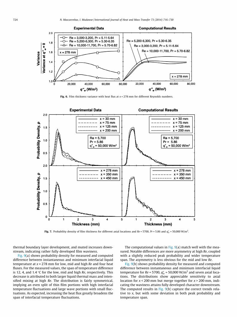
Fig. 6. Film thickness variance with heat flux at x = 278 mm for different Reynolds numbers.

Fig. 7. Probability density of film thickness for different axial locations and Re = 5700, Pr = 5.86 and q00w = 50,000 W/m2.

724 N. Mascarenhas, I. Mudawar / International Journal of Heat and Mass Transfer 73 (2014) 716–730

thermal boundary layer development, and muted increases down-stream, indicating rather fully developed film waviness.

Fig. 9(a) shows probability density for measured and computeddifference between instantaneous and minimum interfacial liquidtemperature at x = 278 mm for low, mid and high Re and four heatfluxes. For the measured values, the span of temperature differenceis 12, 4, and 1.4 �C for the low, mid and high Re, respectively. Thisdecrease is attributed to both larger liquid thermal mass and inten-sified mixing at high Re. The distribution is fairly symmetrical,implying an even split of thin film portions with high interfacialtemperature fluctuations and large wave portions with small fluc-tuations. As expected, increasing the heat flux greatly broadens thespan of interfacial temperature fluctuations.

The computational values in Fig. 9(a) match well with the mea-sured. Notable differences are more asymmetry at high Re, coupledwith a slightly reduced peak probability and wider temperaturespan. The asymmetry is less obvious for the mid and low Re.

Fig. 9(b) shows probability density for measured and computeddifference between instantaneous and minimum interfacial liquidtemperature for Re = 5700, q00w = 50,000 W/m2 and seven axial loca-tions. The distributions show appreciable sensitivity to axiallocation for x < 200 mm but merge together for x > 200 mm, indi-cating the waviness attains fully developed character downstream.The computed results in Fig. 9(b) capture the correct trends rela-tive to x, but with some deviation in both peak probability andtemperature span.

Fig. 8. Variance of film thickness with axial distance for Re = 5700, Pr = 5.86 and q00w = 50,000 W/m2.

Fig. 9. Probability density of difference between instantaneous and minimum interfacial liquid temperature for (a) x = 278 mm and different Reynolds numbers and heatfluxes, and (b) Re = 5700, Pr = 5.86, q00w = 50,000 W/m2 and different axial locations.

N. Mascarenhas, I. Mudawar / International Journal of Heat and Mass Transfer 73 (2014) 716–730 725

4.3. Auto-covariance and cross covariance results

Covariance is a measure of the tendency of two variables toco-vary or ‘‘move’’ together. Following [44], covariance of filmthickness, d, and difference between instantaneous and minimuminterfacial temperature, Ti � Ti,min, is given by

covfd; Ti � Ti;ming ¼1

Nffiffiffiffiffiffir2

d

p ffiffiffiffiffiffiffiffiffiffiffiffiffiffiffiffiffir2

Ti�Ti;min

q XN

j

ðdj � dÞ ðTi � Ti;minÞj�

�ðTi � Ti;minÞ�; ð13Þ

where

r2Ti�Ti;min

¼ 1N

XN

j

ðTi � Ti;minÞj � ðTi � Ti;minÞh i2

ð14Þ

and

Ti � Ti;min ¼1N

XN

j¼1

ðTi � Ti;minÞj: ð15Þ

A positive covariance implies larger values of d are associated withlarger values of Ti � Ti,min, and smaller values of d with smaller

726 N. Mascarenhas, I. Mudawar / International Journal of Heat and Mass Transfer 73 (2014) 716–730

values of Ti � Ti,min. A negative covariance implies smaller values ofd are associated with larger values of Ti � Ti,min, and larger values ofd with smaller values of Ti � Ti,min.

When a process has instantaneous values that are interdepen-dent, the interdependency can be characterized with the aid ofauto-covariance. For a time series, auto-covariance is the covari-ance between values at time t with values at other times. Theauto-covariances of film thickness, d, and difference betweeninstantaneous and minimum interfacial temperature, Ti � Ti,min,for times t and t + s are given, respectively, by Anderson [44]

Rd;dðsÞ ¼ covfdðtÞdðt þ sÞg ð16Þ

and

RTi�Ti;min ; Ti�Ti;minðsÞ ¼ cov Ti � Ti;minðtÞ; Ti � Ti;minðt þ sÞ

� ; ð17Þ

where s is the time ‘‘lag’’. High auto-covariance indicates that theseries changes slowly, or, equivalently, that the present value is pre-dictable from previous values. For example, white noise has a veryflat auto-covariance because it is random, while nature images typ-ically possess broad spatial auto-covariance because nearby pixelsare often of similar color and brightness.

Cross-covariance compares two time series by shifting one intime relative to the other. Cross-covariance between film thicknessand difference between instantaneous and minimum interfacialtemperature is defined as

Cd;Ti�Ti;minðsÞ ¼ covfdðtÞ; Ti � Ti;minðt þ sÞg: ð18Þ

If d and Ti � Ti,min are delayed copies of one another, they will have across-correlation with a peak value of unity at some time lag. Thus,the cross-covariance is useful at capturing how interfacial temper-ature is influenced by interfacial waviness after some time delay.

Both the measured and computational covariance results pre-sented here are means of discrete distributions corresponding tofour data sets of identical operating conditions. The total durationfor each set is 0.4 s.

Fig. 10(a) and (b) show, for the mid and high Re, respectively,both experimental and computational auto-covariance results forfilm thickness, d, and difference between instantaneous and mini-mum interfacial temperature, Ti � Ti,min, and cross-covariance be-tween the two parameters. The experimental auto-covariance ford follows the pattern of a time series with periodic elements[44], starting with a value of unity for s = 0, where the thicknessduplicates itself. A second relatively high positive auto-covariancevalue is achieved for a time lag that corresponds to the dominantwave period. Subsequent time lags that are integral multiples ofthe period are manifest as local maxima that gradually decline inmagnitude. Consequently, local minima occur at time lags corre-sponding to integral multiples of the maximum out of phase value.The auto-covariance plots point to time records of film thicknessthat are periodic, and the phase shift at larger time lags can beattributed to the gradual influence of non-periodic elements. No-tice that the periodicity is strong for both mid and high Re, andthe influence of heat flux is relatively weak. However, non-period-icities for high Re are introduced much earlier, evidenced by the re-duced amplitude for the larger time lags, which can be explainedby the increased turbulence at high Re intensifying stochasticbehavior. Fig. 10(a) and (b) show the computational results agreewell with the measured, however, the maxima and minima areslightly more pronounced for the computed results.

The cross-covariance plots in Fig. 10(a) and (b) show a singlesignificant time lag of positive covariance, followed by a somewhatneutral covariance. But most notable is a pronounced negativecross-covariance between film thickness and interfacial liquidtemperature at about one quarter the wave period from the thick-ness auto-covariance plot. This implies that the liquid temperature

peaks in the relatively thin film region between the film substrateand wave peak, and has a minimum in the relatively thick film re-gion between the wave peak and substrate; both behaviors arecaptured very well in the streamline plot in Fig. 11. Overall,cross-covariance exhibits relatively weak dependence on heat fluxand the computational results show good agreement with themeasured.

Fig. 12(a) and (b) show experimental and computational auto-covariance results for film thickness and difference betweeninstantaneous and minimum interfacial liquid temperature,respectively, for Re = 5,700, Pr = 5.86 and q00w = 50,000 W/m2 at se-ven longitudinal locations. For the most part, the auto-covarianceresults appear to be weakly influenced by x. However, the auto-covariance of film thickness shows stronger correlation forx > 200 mm, which proves that the film attains fully developedwave structure downstream. This trend is not captured in the tem-perature auto-covariance plots. The computed results show stron-ger auto-covariance for both thickness and interfacial temperatureand, like the measured results, exhibit weak sensitivity to x.

4.4. Auto-spectrum and cross-spectrum results

A spectral plot is a graphical data analysis technique that is usedto examine frequency domain models for single or multiple timeseries, and provides an alternate means to assessing covarianceand periodicity. The key approach in spectral analysis is to super-impose sine and cosine profiles with different amplitudes to gener-ate an artificial time series that resembles the actual time series.An examination of the terms that constitute the artificial series al-lows for easier interpretation of the actual time series.

The auto-spectrum function for a given frequency f is obtainedby applying smoothed Fast Fourier Transforms (FFTs) to auto-covariance data [45], which, for film thickness, is given by

Sd;dðf Þ ¼D Rd;dð0Þ½ � þ

PL�1j¼1 Rd;dðjÞwðjÞ cosð2pfjDÞPL�1

j¼1 Rd;dð0Þ cosð2pfjDÞ; ð19Þ

where D, Rd,d, L and w(j) are, respectively, the difference betweenadjacent covariance values, auto-covariance at time lag j, total num-ber of discrete time lags used, and window function that aids in thesmoothing.

The cross-spectrum for film thickness and difference betweeninstantaneous and minimum interfacial liquid temperature is sim-ilarly obtained by applying smoothed FFTs to the cross-covariancedata [45],

STi�Ti;min ;Ti�Ti;minðf Þ¼

D RTi�Ti;min ;Ti�Ti;minð0Þ

h iþPL�1

j¼1 RTi�Ti;min ;Ti�Ti;minðjÞwðjÞcosð2pfjDÞPL�1

j¼1 RTi�Ti;min ;Ti�Ti;minð0Þcosð2pfjDÞ

:

ð20Þ

For the experimental data, the thickness and temperature spec-tra are calculated in the present study following a method previ-ously employed by Karapantsios et al. [15] in analyzing adiabaticfilm thickness data. A Hanning window function is applied to re-duce side-lobe leakage (i.e., filter out noise in the time records)[46]. Spectral results are calculated for each of three segments ofa database using an FFT code written by Newland [47], which arethen averaged. Representative spectra are finally obtained by aver-aging results from four data bases obtained at identical operatingconditions. The computational results are processed by consideringeight covariance sets of 0.4 s intervals and converted to spectralplots using DATAPLOT [48], a statistical analysis tool developedby the National Institute of Standards and Technology (NIST), whichis used in this study to perform the FFT, smoothing and averaging.The Tukey window function used for smoothing and to reduce leak-age is given by [49]

Fig. 10. Auto-covariances of film thickness and difference between instantaneous and minimum interfacial liquid temperature, and corresponding cross-covariance atx = 278 mm for (a) Re = 5300–6300 and Pr = 5.30–6.35, and (b) Re = 10,000–11,700 and Pr = 5.70–6.82.

Fig. 11. Computed liquid flow streamlines and liquid temperature measured at x = 278 mm and y = 0.58 mm for Re = 10,800, Pr = 6.22 and q00w = 50,000 W/m2 (adapted from[5]).

N. Mascarenhas, I. Mudawar / International Journal of Heat and Mass Transfer 73 (2014) 716–730 727

wðuÞ ¼ 12

1þ cospuL

� h i; ð21Þ

and the number of time lags, L, which correlates the width N, insamples, of a discrete-time symmetrical window function w(j), iscalculated as [49]

L ¼ N4� 1: ð22Þ

Fig. 13(a) and (b) show experimental and computational auto-spectra of film thickness and difference between instantaneousand minimum interfacial liquid temperature, normalized by theFFT of their respective variance at zero time lag, and cross-spectrabetween the two parameters, normalized by the product of theFFTs of their respective variance at zero time lag, at x = 278 mmfor different heat fluxes at mid and high Re, respectively. The thick-ness auto-spectra display peak values over a narrow frequency

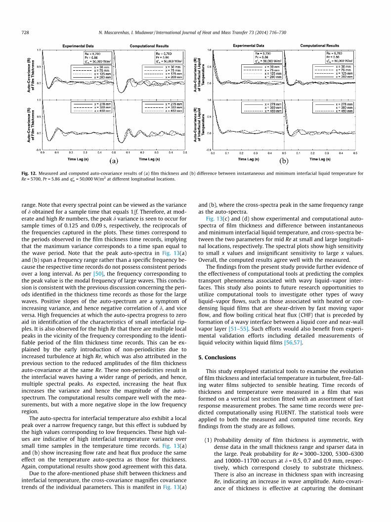
Fig. 12. Measured and computed auto-covariance results of (a) film thickness and (b) difference between instantaneous and minimum interfacial liquid temperature forRe = 5700, Pr = 5.86 and q00w = 50,000 W/m2 at different longitudinal locations.

728 N. Mascarenhas, I. Mudawar / International Journal of Heat and Mass Transfer 73 (2014) 716–730

range. Note that every spectral point can be viewed as the varianceof d obtained for a sample time that equals 1/f. Therefore, at mod-erate and high Re numbers, the peak d variance is seen to occur forsample times of 0.125 and 0.09 s, respectively, the reciprocals ofthe frequencies captured in the plots. These times correspond tothe periods observed in the film thickness time records, implyingthat the maximum variance corresponds to a time span equal tothe wave period. Note that the peak auto-spectra in Fig. 13(a)and (b) span a frequency range rather than a specific frequency be-cause the respective time records do not possess consistent periodsover a long interval. As per [50], the frequency corresponding tothe peak value is the modal frequency of large waves. This conclu-sion is consistent with the previous discussion concerning the peri-ods identified in the thickness time records as those for the largewaves. Positive slopes of the auto-spectrum are a symptom ofincreasing variance, and hence negative correlation of d, and viceversa. High frequencies at which the auto-spectra progress to zeroaid in identification of the characteristics of small interfacial rip-ples. It is also observed for the high Re that there are multiple localpeaks in the vicinity of the frequency corresponding to the identi-fiable period of the film thickness time records. This can be ex-plained by the early introduction of non-periodicities due toincreased turbulence at high Re, which was also attributed in theprevious section to the reduced amplitudes of the film thicknessauto-covariance at the same Re. These non-periodicities result inthe interfacial waves having a wider range of periods, and hence,multiple spectral peaks. As expected, increasing the heat fluxincreases the variance and hence the magnitude of the auto-spectrum. The computational results compare well with the mea-surements, but with a more negative slope in the low frequencyregion.

The auto-spectra for interfacial temperature also exhibit a localpeak over a narrow frequency range, but this effect is subdued bythe high values corresponding to low frequencies. These high val-ues are indicative of high interfacial temperature variance oversmall time samples in the temperature time records. Fig. 13(a)and (b) show increasing flow rate and heat flux produce the sameeffect on the temperature auto-spectra as those for thickness.Again, computational results show good agreement with this data.

Due to the afore-mentioned phase shift between thickness andinterfacial temperature, the cross-covariance magnifies covariancetrends of the individual parameters. This is manifest in Fig. 13(a)

and (b), where the cross-spectra peak in the same frequency rangeas the auto-spectra.

Fig. 13(c) and (d) show experimental and computational auto-spectra of film thickness and difference between instantaneousand minimum interfacial liquid temperature, and cross-spectra be-tween the two parameters for mid Re at small and large longitudi-nal locations, respectively. The spectral plots show high sensitivityto small x values and insignificant sensitivity to large x values.Overall, the computed results agree well with the measured.

The findings from the present study provide further evidence ofthe effectiveness of computational tools at predicting the complextransport phenomena associated with wavy liquid–vapor inter-faces. This study also points to future research opportunities toutilize computational tools to investigate other types of wavyliquid–vapor flows, such as those associated with heated or con-densing liquid films that are shear-driven by fast moving vaporflow, and flow boiling critical heat flux (CHF) that is preceded byformation of a wavy interface between a liquid core and near-wallvapor layer [51–55]. Such efforts would also benefit from experi-mental validation efforts including detailed measurements ofliquid velocity within liquid films [56,57].

5. Conclusions

This study employed statistical tools to examine the evolutionof film thickness and interfacial temperature in turbulent, free-fall-ing water films subjected to sensible heating. Time records ofthickness and temperature were measured in a film that wasformed on a vertical test section fitted with an assortment of fastresponse measurement probes. The same time records were pre-dicted computationally using FLUENT. The statistical tools wereapplied to both the measured and computed time records. Keyfindings from the study are as follows.

(1) Probability density of film thickness is asymmetric, withdense data in the small thickness range and sparser data inthe large. Peak probability for Re = 3000–3200, 5300–6300and 10000–11700 occurs at d = 0.5, 0.7 and 0.9 mm, respec-tively, which correspond closely to substrate thickness.There is also an increase in thickness span with increasingRe, indicating an increase in wave amplitude. Auto-covari-ance of thickness is effective at capturing the dominant

Fig. 13. Auto-spectra of film thickness and difference between instantaneous and minimum interfacial temperature, and corresponding cross-spectra for (a) x = 278 mm,Re = 5300–6,300, Pr = 5.30–6.3 and different heat fluxes, (b) x = 278 mm, Re = 10,000–11,700, Pr = 5.70–6.82 and different heat fluxes, (c) Re = 5300–5500, Pr = 6.08–6.35,q00w = 50,000 W/m2 and different upstream axial locations, and (d) Re = 5300–5500, Pr = 6.08–6.35, q00w = 50,000 W/m2 and different downstream axial locations.

N. Mascarenhas, I. Mudawar / International Journal of Heat and Mass Transfer 73 (2014) 716–730 729

wave period, and proves the film thickness time record isperiodic. The auto-spectrum of film thickness is effective atcapturing the range of dominant frequencies correspondingto the large waves.

(2) Probability density of interfacial temperature is fairly sym-metrical, suggesting nearly equal number of thin substratedata with high interfacial temperature fluctuations and thickwave data with small fluctuations. Increasing Re decreasesthe interfacial temperature difference, a trend attributed to

both larger liquid thermal mass and intensified mixing athigh Re. Increasing the wall heat flux greatly broadens thespan of interfacial temperature fluctuations.

(3) Cross-covariance of film thickness and interfacial tempera-ture difference captures a pronounced negative minimumat about one quarter the dominant wave period. This impliesa clear phase shift between the two parameters, with theliquid temperature reaching a maximum in the relativelythin film region between the substrate and wave peak.

730 N. Mascarenhas, I. Mudawar / International Journal of Heat and Mass Transfer 73 (2014) 716–730

(4) The probability density, covariance and spectra of both thefilm thickness and interfacial temperature difference exhibitclear dependence on axial distance for x < 200 mm, com-pared to insignificant dependence for larger distances. Thesetrends point to a wave structure gradually developing in thethermal entrance region, and a fully developed structuredownstream.

(5) Overall, the statistical results based on computed film thick-ness and interfacial temperature difference agree well withthe results based on the measured. This proves the effective-ness of the adopted computational tools at predicting thecomplex transport phenomena associated with wavyliquid–vapor interfaces.

Acknowledgement

The authors are grateful for the partial support for this projectfrom the National Aeronautics and Space Administration (NASA)under grant no. NNX13AB01G.

References

[1] L.-T. Yeh, R.C. Chu, Thermal Management of Microelectronic Equipment: HeatTransfer Theory, Analysis Methods, and Design Practices, ASME, New York,2002.

[2] T.M. Anderson, I. Mudawar, Microelectronic cooling by enhanced pool boilingof a dielectric fluorocarbon liquid, J. Heat Transfer – Trans. ASME 111 (1989)752–759.

[3] S. Mukherjee, I. Mudawar, Smart pumpless loop for micro-channel electroniccooling using flat and enhanced surfaces, IEEE Trans. Compon. Packag. Technol.26 (2003) 99–109.

[4] S. Mukherjee, I. Mudawar, Pumpless loop for narrow channel and micro-channel boiling from vertical surfaces, J. Electron. Packag. Trans. ASME 125(2003) 431–441.

[5] N. Mascarenhas, I. Mudawar, Study of the influence of interfacial waves onheat transfer in turbulent falling films, Int. J. Heat Mass Transfer 67 (2013)1106–1121.

[6] T.H. Lyu, I. Mudawar, Statistical investigation of the relationship betweeninterfacial waviness and sensible heat transfer to a falling liquid film, Int. J.Heat Mass Transfer 34 (1991) 1451–1464.

[7] N. Mascarenhas, I. Mudawar, Investigation of eddy diffusivity and heat transfercoefficient for free-falling turbulent liquid films subjected to sensible heating,Int. J. Heat Mass Transfer 64 (2013) 647–660.

[8] O.M. Phillips, The equilibrium range in the spectrum of wind-generated waves,J. Fluid Mech. 4 (1958) 426–434.

[9] A.S. Telles, A.E. Dukler, Statistical characteristics of thin, vertical, wavy, liquidfilms, Ind. Eng. Chem. Fundam. 9 (1970) 99–109.

[10] K.J. Chu, A.E. Dukler, Statistical characteristics of thin wavy films: part IIstudies of the substrate and its wave structure, AIChE J. 20 (1974) 695–706.

[11] K.J. Chu, A.E. Dukler, Statistical characteristics of thin wavy films: part IIIstructure of the large waves and their resistance to gas flow, AIChE J. 21 (1975)583–593.

[12] O.C. Jones, J.M. Delhaye, Transient and statistical measurement techniques fortwo-phase flows: a critical review, Int. J. Multiphase Flow 3 (1976) 89–116.

[13] H. Takahama, S. Kato, Longitudinal flow characteristics of vertically fallingliquid films without concurrent gas flow, Int. J. Multiphase Flow 6 (1980) 203–215.

[14] F. Nencini, P. Andreussi, Studies of the behavior of disturbance waves inannular two-phase flow, Can. J. Chem. Eng. 60 (1982) 459–465.

[15] T.D. Karapantsios, S.V. Paras, A.J. Karabelas, Statistical characteristics of freefalling films at high Reynolds numbers, Int. J. Multiphase Flow 15 (1989) 1–21.

[16] W. Ambrosini, N. Forgione, F. Oriolo, Statistical characteristics of a water filmfalling down a flat plate at different inclinations and temperatures, Int. J.Multiphase Flow 28 (2002) 1521–1540.

[17] J.A. Shmerler, I. Mudawar, Local heat transfer coefficient in wavy free-fallingturbulent liquid films undergoing uniform sensible heating, Int. J. Heat MassTransfer 31 (1988) 67–77.

[18] T.H. Lyu, I. Mudawar, Determination of wave-induced fluctuations of walltemperature and convection heat transfer coefficient in the heating of aturbulent falling liquid film, Int. J. Heat Mass Transfer 34 (1991) 2521–2534.

[19] T.H. Lyu, I. Mudawar, Simultaneous measurement of thickness andtemperature profile in a wavy liquid film falling freely on a heating wall,Exp. Heat Transfer 4 (1991) 217–233.

[20] J.A. Shmerler, I. Mudawar, Local evaporative heat transfer coefficient inturbulent free-falling liquid films, Int. J. Heat Mass Transfer 31 (1988) 731–742.

[21] W.J. Marsh, I. Mudawar, Predicting the onset of nucleate boiling in wavy free-falling turbulent liquid films, Int. J. Heat Mass Transfer 32 (1989) 361–378.

[22] R. Walraven, Digital filters, in: Proceedings Digital Equipment Computer UsersSociety, San Diego, CA, 1980, pp. 827–834.

[23] ANSYS FLUENT 12.1 in Workbench User’s Guide. ANSYS Inc., Canonsburg, PA,2009.

[24] F. Gu, C.J. Liu, X.G. Yuan, G.C. Yu, CFD simulation of liquid film flow on inclinedplates, Chem. Eng. Technol. 27 (2004) 1099–1104.

[25] F. Jafar, G. Thorpe, O.F. Turan, Liquid film falling on horizontal circularcylinders, in: Proceedings 16th Australasian Fluid Mech. Conf., Brisbane,Australia, 2007, pp. 1193–1199.

[26] J.F. Xu, B.C. Khoo, N.E. Wijeysundera, Mass transfer across the falling film:simulations and experiments, Chem. Eng. Sci. 63 (2008) 2559–2575.

[27] S. Bo, X. Ma, Z. Lan, J. Chen, H. Chen, Numerical simulation on the falling filmabsorption process in a counter-flow absorber, Chem. Eng. J. 156 (2010) 607–612.

[28] C.-D. Ho, H. Chang, H.-J. Chen, C.-L. Chang, H.-H. Li, Y.-Y. Chang, CFD simulationof the two-phase flow for a falling film microreactor, Int. J. Heat Mass Transfer54 (2011) 3740–3748.

[29] F. Sun, S. Xu, Y. Gao, Numerical simulation of liquid falling film on horizontalcircular tubes, Front. Chem. Sci. Eng. 6 (2012) 322–328.

[30] H. Ganapathy, A. Shooshtari, K. Choo, S. Dessiatoun, M. Alshehhi, M. Ohadi,Volume of fluid-based numerical modeling of condensation heat transfer andfluid flow characteristics in microchannels, Int. J. Heat Mass Transfer 65 (2013)62–72.

[31] O. Reynolds, Study of fluid motion by means of coloured bands, Nature 50(1894) 161–164.

[32] J.O. Hinze, Turbulence, McGraw-Hill, New York, NY, 1975.[33] J.U. Brackbill, D.B. Kothe, C. Zemach, A continuum method for modeling

surface tension, J. Comput. Phys. 100 (1992) 335–354.[34] M. Wolfstein, The velocity and temperature distribution of one-dimensional

flow with turbulence augmentation and pressure gradient, Int. J. Heat MassTransfer 12 (1969) 301–318.

[35] H.C. Chen, V.C. Patel, Near-wall turbulence models for complex flows includingseparation, AIAA J. 26 (1988) 641–648.

[36] T. Jongen, Simulation and modeling of turbulent incompressible flows (Ph.D.Thesis), EPF Lausanne, Lausanne, Switzerland, 1992.

[37] B. Kader, Temperature and concentration profiles in fully turbulent boundarylayers, Int. J. Heat Mass Transfer 24 (1981) 1541–1544.

[38] C.W. Hirt, B.D. Nicholls, Volume of fluid (VOF) method for dynamics of freeboundaries, J. Comput. Phys. 39 (1981) 201–225.

[39] W.M. Kays, Turbulent Prandtl number where are we?, J Heat Transfer Trans.ASME 116 (1994) 284–295.

[40] S. Armsfield, R. Street, The fractional-step method for the Navier–Stokesequations on staggered grids: accuracy of three variations, J. Comput. Phys.153 (1999) 660–665.

[41] H.M. Glaz, J.B. Bell, P. Colella, An analysis of the fractional-step method, J.Comput. Phys. 108 (1993) 51–58.

[42] W. Anderson, D.L. Bonhus, An implicit algorithm for computing turbulentflows on unstructured grids, Comput. Fluids 23 (1994) 1–21.

[43] S.V. Patankar, Numerical Heat Transfer and Fluid Flow, Hemisphere,Washington, DC, 1980.

[44] T.W. Anderson, The Statistical Analysis of Time Series, Wiley, New York, NY,1958.

[45] G.M. Jenkins, D. Watts, Spectral Analysis and its Applications, Holden-Day, SanFrancisco, CA, 1968.

[46] D.E. Newland, An Introduction to Random Vibrations and Spectral Analysis,second ed., Longman, New York, NY, 1984.

[47] J.E. Koskie, I. Mudawar, W.G. Tiederman, Parallel-wire probes formeasurement of thick liquid films, Int. J. Multiphase Flow 15 (1989) 521–530.

[48] J. Filliben, Dataplot—an interactive high level, language for graphics non-linearfitting, data analysis, and mathematics, in: Proceeding Third Annual Conf.National Computer Graphics Assoc., Anaheim, CA, 1982.

[49] J. Tukey, Exploratory Data Analysis, Addison-Wesley, New York, NY, 1979.[50] H.T. Davis, Statistical Mechanics of Phases, Interfaces, and Thin Films, Wiley,

New York, NY, 1996.[51] C.O. Cersey, I. Mudawar, Effects of heater length and orientation on the trigger

mechanism for near-saturated flow boiling critical heat flux – I. Photographicstudy and statistical characterization of the near-wall interfacial features, Int.J. Heat Mass Transfer 38 (1995) 629–641.

[52] C.O. Cersey, I. Mudawar, Effects of heater length and orientation on the triggermechanism for near-saturated flow boiling critical heat flux – II. Critical heatflux model, Int. J. Heat Mass Transfer 38 (1995) 643–654.

[53] J.C. Sturgis, I. Mudawar, Critical heat flux in a long, rectangular channelsubjected to onesided heating – I. Flow visualization, Int. J. Heat Mass Transfer42 (1999) 1835–1847.

[54] J.C. Sturgis, I. Mudawar, Critical heat flux in a long, rectangular channelsubjected to onesided heating – II. Analysis of critical heat flux data, Int. J. HeatMass Transfer 42 (1999) 1849–1862.

[55] H. Zhang, I. Mudawar, M.M. Hasan, Flow boiling CHF in microgravity, Int. J.Heat Mass Transfer 48 (2005) 3107–3118.

[56] I. Mudawar, R.A. Houpt, Mass and momentum transport in smooth fallingliquid films laminarized at relatively high Reynolds numbers, Int. J. Heat MassTransfer 36 (1993) 3437–3448.

[57] I. Mudawar, R.A. Houpt, Measurement of mass and momentum transport inwavy-laminar falling liquid films, Int. J. Heat Mass Transfer 36 (1993) 4151–4162.