International Journal of Heat and Mass Transfer 54 (2011) 4560–4569

Contents lists available at ScienceDirect

International Journal of Heat and Mass Transfer

journal homepage: www.elsevier .com/locate / i jhmt

Assessment of an active-cooling micro-channel heat sink device, usingelectro-osmotic flow

Marwan F. Al-Rjoub a, Ajit K. Roy b, Sabyasachi Ganguli b,c, Rupak K. Banerjee a,⇑a School of Dynamic Systems, University of Cincinnati, Cincinnati, OH, USAb Thermal Sciences and Materials Branch (AFRL/RXBT), Air Force Research Laboratory, WPAFB, OH, USAc University of Dayton Research Institute, Dayton, OH, USA

a r t i c l e i n f o a b s t r a c t

Article history:Received 7 February 2011Received in revised form 10 June 2011Accepted 10 June 2011Available online 6 July 2011

Keywords:Electro-osmotic flowMicro-scale heat exchangerHot spot coolingZeta-potentialEOF

0017-9310/$ - see front matter Published by Elsevierdoi:10.1016/j.ijheatmasstransfer.2011.06.022

⇑ Corresponding author. Address: 593 Rhodes HallUniversity of Cincinnati, Cincinnati, OH 45221, USA. Te(513) 556 3390.

E-mail address: rupak.banerjee@uc.edu (R.K. Bane

Non-uniform heat flux generated by microchips causes ‘‘hot spots’’ in very small areas on the microchipsurface. These hot spots are generated by the logic blocks in the microchip bay; however, memory blocksgenerate lower heat flux on contrast. The goal of this research is to design, fabricate, and test an activecooling micro-channel heat sink device that can operate under atmospheric pressure while achievinghigh-heat dissipation rate with a reduced chip-backside volume, particularly for spot cooling applica-tions. An experimental setup was assembled and electro-osmotic flow (EOF) was used thus eliminatinghigh pressure pumping system. A flow rate of 82 lL/min was achieved at 400 V of applied EOF voltage.An increase in the cooling fluid (buffer) temperature of 9.6 �C, 29.9 �C, 54.3 �C, and 80.1 �C was achievedfor 0.4 W, 1.2 W, 2.1 W, and 4 W of heating powers, respectively. The substrate temperature at the middleof the microchannel was below 80.5 �C for all input power values. The maximum increase in the coolingfluid temperature due to the joule heating was 4.5 �C for 400 V of applied EOF voltage. Numerical calcu-lations of temperatures and flow were conducted and the results were compared to experimental data.Nusselt number (Nu) for the 4 W case reached a maximum of 5.48 at the channel entrance and decreasedto reach 4.56 for the rest of the channel. Nu number for EOF was about 10% higher when compared to thepressure driven flow. It was found that using a shorter channel length and an EOF voltage in the range of400–600 V allows application of a heat flux in the order of 104 W/m2, applicable to spot cooling. For ele-vated voltages, the velocity due to EOF increased, leading to an increase in total heat transfer for a fixedduration of time; however, the joule heating also got elevated with increase in voltage.

Published by Elsevier Ltd.

1. Introduction

Intensive computing devices are projected to generate heat fluxvalues that can exceed 2.5 � 106 W/m2 [1]. With these high-heatgeneration rates the conventional cooling techniques have beenfound to be inadequate. Instead of forcing air to flow over fins, li-quid can be forced to flow through channels that are in contactwith the devices’ surface. Various methods are being used to drivea liquid through micro-channels, which include pressure driventechniques that use mechanical pumps or pressurized gases. An-other approach is to use electro-osmotic flow pumping technique;this technique has no moving parts and needs less maintenancecompared to mechanical pumps.

Ltd.

, School of Dynamic Systems,l.: +1 (513) 556 2124; fax: +1

rjee).

1.1. Electro-osmotic flow (EOF)

Solid surfaces develop a charge when brought into contact withan aqueous solution [2]. Due to the formation of surface charge,counter ions in the solution will be attracted toward the surface.The concentration of counter ions in the vicinity of the surface willbe higher than in the fluid bulk, whereas co-ions concentration inthe fluid bulk is higher than its concentration in the vicinity of thesurface. The charged surface and the thin layer of counter ions thatbalances its charge are defined as the electric double layer (EDL)[2].

Ions in the vicinity of the charged surface are attracted to itand this restricts their motion (immobile ions). Ions away fromthe charged surface are not strongly affected by the charged sur-face. This leads to a higher mobility (mobile ions). When an elec-tric field is applied between two points of the aqueous solution,the mobile ions start to move under the influence of the electricfield. The ions motion drags other fluid particles due to viscousforces. This leads to a bulk fluid motion known as electro-osmoticflow.

Nomenclature

Across cross sectional area of the channel, m2

B bias errorDAQ data acquisition systemDI de-ionizedE electric field, V/mEDL electric double layerEOF electro-osmotic flowh heat transfer coefficient, W/m2 Khi Cooling fluid (buffer enthalpy) at the channel inlet, J/kgho cooling fluid (buffer enthalpy) at the channel outlet, J/kgm mass, kgp pressure, PaP precision errorPDMS polydimethyl siloxaneT temperature

u internal energy, J/kg~u velocity, m/sU total uncertainty

Greek symbolsaf cooling fluid (buffer) diffusivitye permittivity, C/V mU applied voltage, Vw wall surface charge, C/m2

l water viscosity, Pa sk bulk conductivity, S/mq energy loss from the reservoir, Jq density, kg/m3

qe bulk charge density, C/m3

f zeta potential, V

M.F. Al-Rjoub et al. / International Journal of Heat and Mass Transfer 54 (2011) 4560–4569 4561

Jiang et al. [3] designed a closed-loop two-phase micro-channelcooling system with an external EOF pump and a heat rejecter, amaximum of 7 ml/min coolant flow rate was achieved, with a chiptemperature maintained less than 120 �C. Laser et al. [4] used theEOF through narrow deep micro-channels to reduce the tempera-ture of the high-power density spots of microchips, 170 lL/minof coolant flow was achieved at 400 V of applied EOF voltage.Zhang et al. [5] tested a single micro-channel for the pressure dis-tribution along the heating length and measured the temperaturevariations during the phase change, the flow was pressure drivenusing a syringe pump. Jung et al. [6] used a single micro-channelto study the heat transfer to nanofluids, and investigated the differ-ences between nanofluids and pure water for convection heattransfer coefficient and friction factor. Eng et al. [7] designed anelectro-osmotic flow silicon-based heat spreader that generated acoolant flow rate of 0.2 lL/min at 2 V/mm electric field; a 4 �Creduction in device temperature was achieved.

Tiselj et al. [8] studied the effect of axial conduction on heattransfer in micro-channels, where experimental and numerical ap-proaches were adopted. It was shown that the bulk fluid and thechannel walls’ temperatures do not vary lineally along the channel.The most significant changes in the temperature gradient were re-ported in the axial flow direction. In the flow direction the effect ofaxial heat flux was maximum at the channel inlet and minimum atoutlet. Yin and Bau [9] studied the performance of micro-heatexchangers theoretically. The micro-heat exchanger was optimizedto achieve a minimum heat resistance. Gillot et al. [10] designed amicro-heat sink to handle the heat generated by a module of insu-lated gate bipolar transistor (IGBT); a thermal resistance of 0.08–0.12 K/W was achieved for the module of IGBT chips.

Sze et al. [11] measured the zeta-potential for an electro-osmo-tic flow in a parallel plate micro-channel. Using Smoluchowskiequation and current time relationship, zeta potentials for glassand PDMS were evaluated. Husain and Kim [12] numerically stud-ied the performance of an EOF driven flow and a pressure drivenflow in a microchannel heat sink with wavy channels. The studyshowed an increase in heat transfer to the cooling fluid for thepressure driven flow due to recirculation. They found that applyingEOF flow increased the flow rate but eliminated the effect of chan-nel waviness due to its uniform flow profile. Dasgupta et al. [13] ofour group studied the effects of the applied-electric field and mi-cro-channel wetted-perimeter on electro-osmotic velocity. Thesenumerical and experimental studies found that, as the wettedperimeter increases, the electro-osmotic velocity decreases, andthe electro-osmotic velocity increases as the applied electric fieldincreases.

Studies of heat removal techniques using fluid flow through mi-cro-channels, reported in recent literature, can be classified intothree main pumping categories, which are pressure driven pump,external EOF pump, and integrated EOF pump. These are identifiedby the type of technique used to drive the fluid flow through themicro-channels. In the case of pressure driven flow, fluid is forcedthrough the channels by an external mechanical pump or com-pressed gas. An external EOF pump can also be used to drive thefluid flow through electrically charged micro-channels. The mi-cro-channels of the heat removal device can itself be used as anintegrated EOF pump. For devices that fall in the first two catego-ries, there is the need for an external pump that occupies largervolume and needs higher power for its operation. For devices thatfall in the third category, the electrically charged microchannelsserve both as a heat exchanger and an integrated pump. Hencethe volume and power requirement are reduced. The maximumheat flux removal capacity and the cooling fluid flow rate for thethree categories vary. A brief comparison between the coolingcapacities of the three categories is presented in the followingparagraphs.

1.2. Pressure driven flow

A recent study by Chiu et al. [14] used a pressure driven flowwhich removed a maximum heat flux of 1.57 � 105 W/m2. Themaximum flow rate of the cooling fluid was 300 ml/min. In anotherstudy by Ornatskii and Viyarskii [15] the maximum heat flux re-moved using micro-channel fluid flow was 4 � 107 W/m2. Due tothe higher flow rates of the cooling fluid, pressure driven flowsare typically capable of removing higher heat flux values. The con-vective heat transfer due to pressure driven flow is typically limitedby the parabolic nature of the velocity profile in the developed re-gion. Due to the size and power limitations of modern electronic de-vices, such pressure driven pump has major challenges because ofthe high operating pressure needing better sealing mechanism, lar-ger pump size, and higher pumping power. The reliability of such asystem with moving parts is a major operational issue.

1.3. External EOF pump

Using an external EOF pump Jiang et al. [3] removed a3.8 � 105 W/m2 of heat flux and achieved a maximum cooling fluidflow rate of 4 ml/min. This system eliminated the need of highpressure mechanical pump and replaced it with an EOF pump.While such external EOF pumping system can be more reliable

4562 M.F. Al-Rjoub et al. / International Journal of Heat and Mass Transfer 54 (2011) 4560–4569

than mechanical pumps, it could not adequately reduce the size ofthe system.

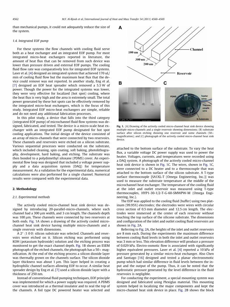
Fig. 1. (A) Drawing of the actively cooled micro-channel heat sink device showingmultiple micro-channels and a single reservoir showing dimensions; (B) substratesurface after silicon etching showing one reservoir and some channels (50�magnification); and (C) photograph of the actively cooled micro-channel heat sinkdevice.

1.4. Integrated EOF pump

For these systems the flow channels with cooling fluid serveboth as a heat exchanger and an integrated EOF pump. For mostintegrated micro-heat exchangers reported in literature, theamount of heat flux that can be removed from such device waslower than pressure driven and external EOF pumps. The coolingfluid flow rate was comparatively less for integrated EOF systems.Laser et al. [4] designed an integrated system that achieved 170 uL/min of cooling fluid flow but the maximum heat flux that the de-vice could remove was not reported. In another study, Eng et al.[7] designed an EOF heat spreader which removed a 5.5 W ofpower. Though the power for the integrated systems was lower,they were very effective for localized (hot spot) cooling, wherethe heat flux is very high and the area is extremely small. The totalpower generated by these hot spots can be effectively removed bythe integrated micro-heat exchangers, which is the focus of thisstudy. Integrated EOF micro-heat exchangers are simple, reliableand do not need any additional fabrication processes.

In this pilot study, a device that falls into the third category(integrated EOF pump) of microchannel fluid flow systems was de-signed, fabricated, and tested. The device is a micro-scale heat ex-changer with an integrated EOF pump designated for hot spotcooling applications. The initial design of the device consisted ofan array of micro-channels that were connected by two reservoirs.These channels and reservoirs were etched on a silicon substrate.Various sequential processes were conducted on the substrate,which included cleaning, spin coating, soft baking, photolithogra-phy, development, hard baking, and etching. The substrate wasthen bonded to a polydimethyl siloxane (PDMS) cover. An experi-mental flow loop was designed that included a voltage power sup-ply and a data acquisition system (DAQ) for temperaturemeasurement. As a validation for the experimental data, numericalcalculations were also performed for a single channel. Numericalresults were compared with the experimental data.

2. Methodology

2.1. Experimental methods

The actively cooled micro-channel heat sink device was de-signed by introducing 20-parallel-micro-channels, where eachchannel had a 300 lm width, and 3 cm length. The channels depthwas 100 lm. These channels were connected by two reservoirs atboth ends. Fig. 1A shows a drawing of the actively cooled micro-channel heat sink device having multiple micro-channels and asingle reservoir with dimensions.

A 200 h1 0 0i silicon substrate was selected. Channels and reser-voirs were etched on it. Silicon etching was performed usingKOH (potassium hydroxide) solution and the etching process wasmonitored to get the exact channel depth. Fig. 1B shows an ESEMphotograph of the etched channels, the photograph has a 50�mag-nification. At the end of the etching process a silicon dioxide layerwas thermally grown on the channels surface. The silicon dioxidelayer thickness was about 1 lm. This layer helped in creating ahydrophilic channel surfaces allowing EOF to occur. A similar heatspreader design by Eng et al. [7] used a silicon dioxide layer with athickness of 250 nm.

Instead of conventional fluid pumping techniques, EOF principlewas implemented for which a power supply was required. A PDMScover was introduced as a thermal insulator and to seal the top ofthe channels. A foil type DC powered heater was selected and

attached to the bottom surface of the substrate. To vary the heatflux, a variable voltage DC power supply was used to power theheater. Voltages, currents, and temperatures were recorded usinga DAQ system. A photograph of the actively cooled micro-channelheat sink device is shown in Fig. 1C. The wires, shown in Fig. 1C,were connected to a DC heater and to a thermocouple that wasattached to the bottom surface of the silicon substrate. A T-typesurface thermocouple [SA1XL-T (Omega Engineering, Inc.)] wasused to measure the substrate temperature at the middle of themicrochannel heat exchanger. The temperature of the cooling fluidat the inlet and outlet reservoir was measured using T-typethermocouples, HYP1-30-1/2-T-G-60-SMWPW-M (Omega Engi-neering, Inc.).

The EOF was applied to the cooling fluid (buffer) using two plat-inum (99.95%) electrodes; the electrodes were wires with circularcross section of 0.5 mm diameter and 12.5 cm length. The elec-trodes were immersed at the center of each reservoir withouttouching the top surface of the silicone substrate. The dimensionsand configuration of the inlet and outlet cooling fluid reservoirs areshown in Fig. 2A.

Referring to Fig. 2A, the heights of the inlet and outlet reservoirsare 8 mm each. During the experiments the maximum differencebetween cooling fluid levels in both the inlet and outlet reservoirswas 3 mm or less. This elevation difference will produce a pressureof 0.029 kPa. Electro-osmotic flow is associated with significantlyhigher equivalent pressures. Laser et al. [4] reported a 10 kPa ofpressure generated by a similar micro-heat exchanger. Also Chenand Santiago [16] designed and tested a planar electroosmoticpump which had similar difference in fluid levels between the in-put and the output of the pump. Thus, it can be noted that thehydrostatic pressure generated by the level difference in the fluidreservoirs is negligible.

For conducting the experiment, a special mounting system wasdesigned and fabricated using Plexiglas material. This mountingsystem helped in localizing the major components and kept themicro-channel heat sink device in place. Fig. 2B shows the block

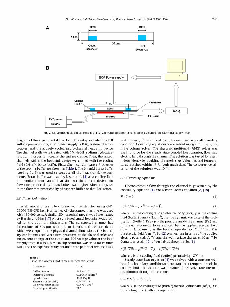
Fig. 2. (A) Configuration and dimensions of inlet and outlet reservoirs and (B) block diagram of the experimental flow loop.

M.F. Al-Rjoub et al. / International Journal of Heat and Mass Transfer 54 (2011) 4560–4569 4563

diagram of the experimental flow loop. The setup included the EOFvoltage power supply, a DC power supply, a DAQ system, thermo-couples, and the actively cooled micro-channel heat sink device.The channel walls were treated with 1M NaOH (sodium hydroxide)solution in order to increase the surface charge. Then, the micro-channels within the heat sink device were filled with the coolingfluid (0.4 mM borax buffer, Ricca Chemical Company). Propertiesof the cooling buffer are shown in Table 1. The 0.4 mM borax buffer(cooling fluid) was used to conduct all the heat transfer experi-ments. Borax buffer was used by Laser et al. [4] as a cooling fluidin a similar microchannel heat sink. For the current design, theflow rate produced by borax buffer was higher when comparedto the flow rate produced by phosphate buffer or distilled water.

2.2. Numerical methods

A 3D model of a single channel was constructed using CFD-GEOM (ESI-CFD Inc., Huntsville, AL). Structured meshing was usedwith 180,000 cells. A similar 3D numerical model was investigatedby Husain and Kim [17] where a microchannel heat sink was stud-ied for the optimum dimensions. The constructed channel haddimensions of 300 lm width, 3 cm length, and 100 lm depthwhich were equal to the physical channel dimensions. The bound-ary conditions used were zero pressures at the channel inlet andoutlet, zero voltage at the outlet and EOF voltage value at the inletranging from 100 to 400 V. No slip condition was used for channelwalls and the experimentally obtained zeta potential was used as a

Table 1List of the properties used in the numerical calculations.

Parameter Value

Buffer density 997 kg m-3

Dynamic viscosity 0.000855 N s m�2

Specific heat 4181 J/kg KThermal conductivity 0.58 W/m KElectrical conductivity 0.00766 S m�1

Relative permittivity 78.5

wall property. Constant wall heat flux was used as a wall boundarycondition. Governing equations were solved using a multi-physicsfinite volume solver. The algebraic multi-grid (AMG) solver wasused to solve for the steady state coupled heat transfer, flow, andelectric field through the channel. The solution was tested for meshindependency by doubling the mesh size. Velocities and tempera-tures matched within 1% for both mesh sizes. The convergence cri-terion of the solutions was 10�6.

2.3. Governing equations

Electro-osmotic flow through the channel is governed by thecontinuity equation (1) and Navier–Stokes equation (2) [18]

r �~u ¼ 0 ð1Þ

qð~u � r~uÞ ¼ lr2~u�rpþ~f e ð2Þ

where ~u is the cooling fluid (buffer) velocity (m/s), q is the coolingfluid (buffer) density (kg/m3), l is the dynamic viscosity of the cool-ing fluid (buffer) (Pa s), p is the pressure inside the channel (Pa), and~f e is electro-osmotic force induced by the applied electric field(~f e ¼ qe �~E, where qe is the bulk charge density, C m�3 and E isthe electric field, V m�1). Eq. (2) was written in terms of the appliedelectric potential, U, (V) and the wall surface charge, w, (C m�2) byComandur et al. [19] of our lab as shown in Eq. (3)

qð~u � r~uÞ ¼ lr2~u�rpþ �ðr2wþrUÞ ð3Þ

where e is the cooling fluid (buffer) permittivity (C/V m).Steady state heat equation (4) was solved with a constant wall

heat flux boundary condition at a constant inlet temperature of thecooling fluid. The solution was obtained for steady state thermaldistribution through the channel

0 ¼ afr2T �~u � rðTÞ ð4Þ

where af is the cooling fluid (buffer) thermal diffusivity (m2/s), T isthe cooling fluid (buffer) temperature.

4564 M.F. Al-Rjoub et al. / International Journal of Heat and Mass Transfer 54 (2011) 4560–4569

3. Results

The results are presented in three major subsections. First, usingexperimental data, calculation of zeta potential is presented forsubsequent assessment of the EOF characteristics using numericaltechnique. Second, the cooling fluid (buffer) flow rate and velocityare presented and discussed. Third, the outlet cooling fluid temper-ature with change in power is discussed. While presenting thecooling fluid temperature data, the influence of voltage differenceand associated joule heating on EOF and heat transfer is discussed.Subsequently, Nusselt number was calculated and plotted versusthe non-dimensional channel length.

3.1. Calculation of zeta potential (f) and bulk conductivity (k)

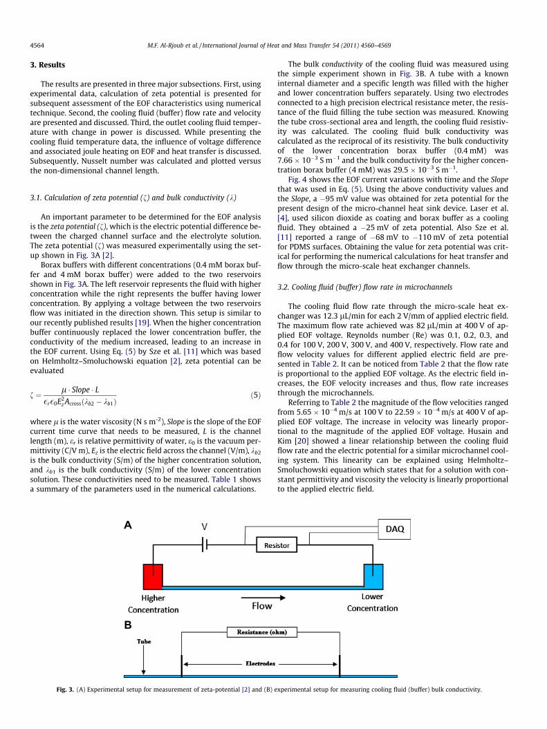
An important parameter to be determined for the EOF analysisis the zeta potential (f), which is the electric potential difference be-tween the charged channel surface and the electrolyte solution.The zeta potential (f) was measured experimentally using the set-up shown in Fig. 3A [2].

Borax buffers with different concentrations (0.4 mM borax buf-fer and 4 mM borax buffer) were added to the two reservoirsshown in Fig. 3A. The left reservoir represents the fluid with higherconcentration while the right represents the buffer having lowerconcentration. By applying a voltage between the two reservoirsflow was initiated in the direction shown. This setup is similar toour recently published results [19]. When the higher concentrationbuffer continuously replaced the lower concentration buffer, theconductivity of the medium increased, leading to an increase inthe EOF current. Using Eq. (5) by Sze et al. [11] which was basedon Helmholtz–Smoluchowski equation [2], zeta potential can beevaluated

f ¼ l � Slope � L�r�0E2

z Acrossðkb2 � kb1Þð5Þ

where l is the water viscosity (N s m-2), Slope is the slope of the EOFcurrent time curve that needs to be measured, L is the channellength (m), er is relative permittivity of water, e0 is the vacuum per-mittivity (C/V m), Ez is the electric field across the channel (V/m), kb2

is the bulk conductivity (S/m) of the higher concentration solution,and kb1 is the bulk conductivity (S/m) of the lower concentrationsolution. These conductivities need to be measured. Table 1 showsa summary of the parameters used in the numerical calculations.

Fig. 3. (A) Experimental setup for measurement of zeta-potential [2] and (B) e

The bulk conductivity of the cooling fluid was measured usingthe simple experiment shown in Fig. 3B. A tube with a knowninternal diameter and a specific length was filled with the higherand lower concentration buffers separately. Using two electrodesconnected to a high precision electrical resistance meter, the resis-tance of the fluid filling the tube section was measured. Knowingthe tube cross-sectional area and length, the cooling fluid resistiv-ity was calculated. The cooling fluid bulk conductivity wascalculated as the reciprocal of its resistivity. The bulk conductivityof the lower concentration borax buffer (0.4 mM) was7.66 � 10�3 S m�1 and the bulk conductivity for the higher concen-tration borax buffer (4 mM) was 29.5 � 10�3 S m�1.

Fig. 4 shows the EOF current variations with time and the Slopethat was used in Eq. (5). Using the above conductivity values andthe Slope, a �95 mV value was obtained for zeta potential for thepresent design of the micro-channel heat sink device. Laser et al.[4], used silicon dioxide as coating and borax buffer as a coolingfluid. They obtained a �25 mV of zeta potential. Also Sze et al.[11] reported a range of �68 mV to �110 mV of zeta potentialfor PDMS surfaces. Obtaining the value for zeta potential was crit-ical for performing the numerical calculations for heat transfer andflow through the micro-scale heat exchanger channels.

3.2. Cooling fluid (buffer) flow rate in microchannels

The cooling fluid flow rate through the micro-scale heat ex-changer was 12.3 lL/min for each 2 V/mm of applied electric field.The maximum flow rate achieved was 82 lL/min at 400 V of ap-plied EOF voltage. Reynolds number (Re) was 0.1, 0.2, 0.3, and0.4 for 100 V, 200 V, 300 V, and 400 V, respectively. Flow rate andflow velocity values for different applied electric field are pre-sented in Table 2. It can be noticed from Table 2 that the flow rateis proportional to the applied EOF voltage. As the electric field in-creases, the EOF velocity increases and thus, flow rate increasesthrough the microchannels.

Referring to Table 2 the magnitude of the flow velocities rangedfrom 5.65 � 10�4 m/s at 100 V to 22.59 � 10�4 m/s at 400 V of ap-plied EOF voltage. The increase in velocity was linearly propor-tional to the magnitude of the applied EOF voltage. Husain andKim [20] showed a linear relationship between the cooling fluidflow rate and the electric potential for a similar microchannel cool-ing system. This linearity can be explained using Helmholtz–Smoluchowski equation which states that for a solution with con-stant permittivity and viscosity the velocity is linearly proportionalto the applied electric field.

xperimental setup for measuring cooling fluid (buffer) bulk conductivity.

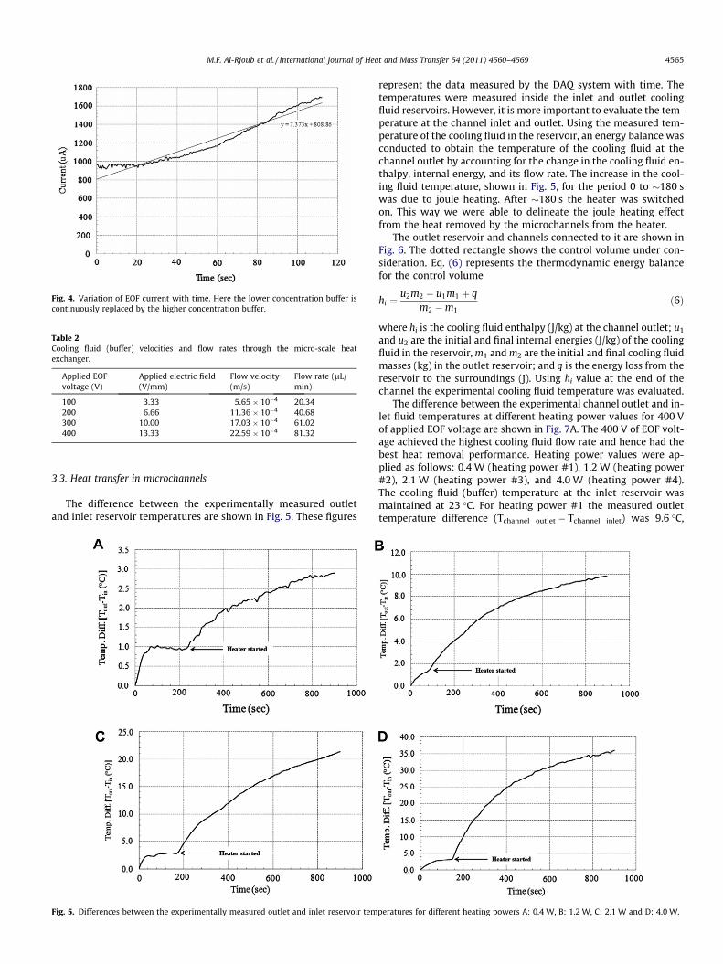
Fig. 4. Variation of EOF current with time. Here the lower concentration buffer iscontinuously replaced by the higher concentration buffer.

Table 2Cooling fluid (buffer) velocities and flow rates through the micro-scale heatexchanger.

Applied EOFvoltage (V)

Applied electric field(V/mm)

Flow velocity(m/s)

Flow rate (lL/min)

100 3.33 5.65 � 10�4 20.34200 6.66 11.36 � 10�4 40.68300 10.00 17.03 � 10�4 61.02400 13.33 22.59 � 10�4 81.32

M.F. Al-Rjoub et al. / International Journal of Heat and Mass Transfer 54 (2011) 4560–4569 4565

3.3. Heat transfer in microchannels

The difference between the experimentally measured outletand inlet reservoir temperatures are shown in Fig. 5. These figures

Fig. 5. Differences between the experimentally measured outlet and inlet reservoir tem

represent the data measured by the DAQ system with time. Thetemperatures were measured inside the inlet and outlet coolingfluid reservoirs. However, it is more important to evaluate the tem-perature at the channel inlet and outlet. Using the measured tem-perature of the cooling fluid in the reservoir, an energy balance wasconducted to obtain the temperature of the cooling fluid at thechannel outlet by accounting for the change in the cooling fluid en-thalpy, internal energy, and its flow rate. The increase in the cool-ing fluid temperature, shown in Fig. 5, for the period 0 to �180 swas due to joule heating. After �180 s the heater was switchedon. This way we were able to delineate the joule heating effectfrom the heat removed by the microchannels from the heater.

The outlet reservoir and channels connected to it are shown inFig. 6. The dotted rectangle shows the control volume under con-sideration. Eq. (6) represents the thermodynamic energy balancefor the control volume

hi ¼u2m2 � u1m1 þ q

m2 �m1ð6Þ

where hi is the cooling fluid enthalpy (J/kg) at the channel outlet; u1

and u2 are the initial and final internal energies (J/kg) of the coolingfluid in the reservoir, m1 and m2 are the initial and final cooling fluidmasses (kg) in the outlet reservoir; and q is the energy loss from thereservoir to the surroundings (J). Using hi value at the end of thechannel the experimental cooling fluid temperature was evaluated.

The difference between the experimental channel outlet and in-let fluid temperatures at different heating power values for 400 Vof applied EOF voltage are shown in Fig. 7A. The 400 V of EOF volt-age achieved the highest cooling fluid flow rate and hence had thebest heat removal performance. Heating power values were ap-plied as follows: 0.4 W (heating power #1), 1.2 W (heating power#2), 2.1 W (heating power #3), and 4.0 W (heating power #4).The cooling fluid (buffer) temperature at the inlet reservoir wasmaintained at 23 �C. For heating power #1 the measured outlettemperature difference (Tchannel outlet � Tchannel inlet) was 9.6 �C,

peratures for different heating powers A: 0.4 W, B: 1.2 W, C: 2.1 W and D: 4.0 W.

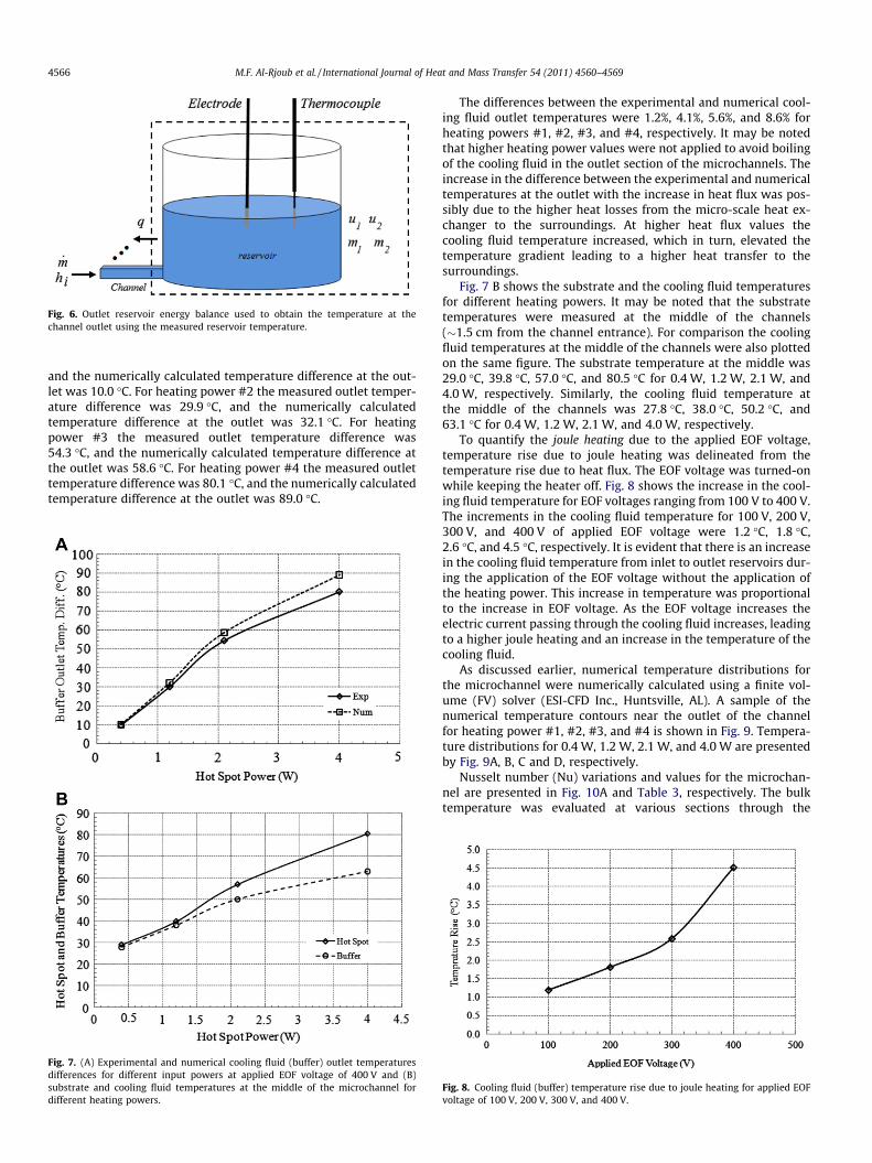
Fig. 6. Outlet reservoir energy balance used to obtain the temperature at thechannel outlet using the measured reservoir temperature.

4566 M.F. Al-Rjoub et al. / International Journal of Heat and Mass Transfer 54 (2011) 4560–4569

and the numerically calculated temperature difference at the out-let was 10.0 �C. For heating power #2 the measured outlet temper-ature difference was 29.9 �C, and the numerically calculatedtemperature difference at the outlet was 32.1 �C. For heatingpower #3 the measured outlet temperature difference was54.3 �C, and the numerically calculated temperature difference atthe outlet was 58.6 �C. For heating power #4 the measured outlettemperature difference was 80.1 �C, and the numerically calculatedtemperature difference at the outlet was 89.0 �C.

Fig. 7. (A) Experimental and numerical cooling fluid (buffer) outlet temperaturesdifferences for different input powers at applied EOF voltage of 400 V and (B)substrate and cooling fluid temperatures at the middle of the microchannel fordifferent heating powers.

The differences between the experimental and numerical cool-ing fluid outlet temperatures were 1.2%, 4.1%, 5.6%, and 8.6% forheating powers #1, #2, #3, and #4, respectively. It may be notedthat higher heating power values were not applied to avoid boilingof the cooling fluid in the outlet section of the microchannels. Theincrease in the difference between the experimental and numericaltemperatures at the outlet with the increase in heat flux was pos-sibly due to the higher heat losses from the micro-scale heat ex-changer to the surroundings. At higher heat flux values thecooling fluid temperature increased, which in turn, elevated thetemperature gradient leading to a higher heat transfer to thesurroundings.

Fig. 7 B shows the substrate and the cooling fluid temperaturesfor different heating powers. It may be noted that the substratetemperatures were measured at the middle of the channels(�1.5 cm from the channel entrance). For comparison the coolingfluid temperatures at the middle of the channels were also plottedon the same figure. The substrate temperature at the middle was29.0 �C, 39.8 �C, 57.0 �C, and 80.5 �C for 0.4 W, 1.2 W, 2.1 W, and4.0 W, respectively. Similarly, the cooling fluid temperature atthe middle of the channels was 27.8 �C, 38.0 �C, 50.2 �C, and63.1 �C for 0.4 W, 1.2 W, 2.1 W, and 4.0 W, respectively.

To quantify the joule heating due to the applied EOF voltage,temperature rise due to joule heating was delineated from thetemperature rise due to heat flux. The EOF voltage was turned-onwhile keeping the heater off. Fig. 8 shows the increase in the cool-ing fluid temperature for EOF voltages ranging from 100 V to 400 V.The increments in the cooling fluid temperature for 100 V, 200 V,300 V, and 400 V of applied EOF voltage were 1.2 �C, 1.8 �C,2.6 �C, and 4.5 �C, respectively. It is evident that there is an increasein the cooling fluid temperature from inlet to outlet reservoirs dur-ing the application of the EOF voltage without the application ofthe heating power. This increase in temperature was proportionalto the increase in EOF voltage. As the EOF voltage increases theelectric current passing through the cooling fluid increases, leadingto a higher joule heating and an increase in the temperature of thecooling fluid.

As discussed earlier, numerical temperature distributions forthe microchannel were numerically calculated using a finite vol-ume (FV) solver (ESI-CFD Inc., Huntsville, AL). A sample of thenumerical temperature contours near the outlet of the channelfor heating power #1, #2, #3, and #4 is shown in Fig. 9. Tempera-ture distributions for 0.4 W, 1.2 W, 2.1 W, and 4.0 W are presentedby Fig. 9A, B, C and D, respectively.

Nusselt number (Nu) variations and values for the microchan-nel are presented in Fig. 10A and Table 3, respectively. The bulktemperature was evaluated at various sections through the

Fig. 8. Cooling fluid (buffer) temperature rise due to joule heating for applied EOFvoltage of 100 V, 200 V, 300 V, and 400 V.

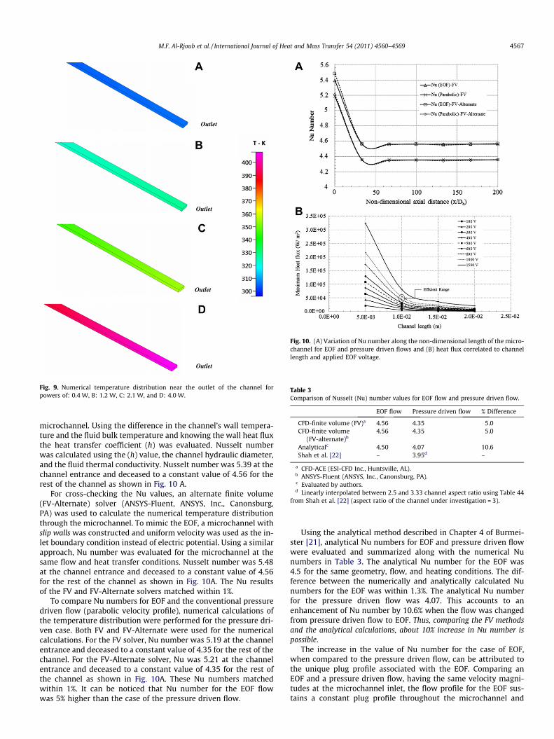
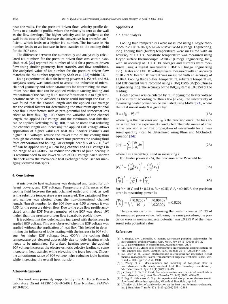
Fig. 10. (A) Variation of Nu number along the non-dimensional length of the micro-channel for EOF and pressure driven flows and (B) heat flux correlated to channellength and applied EOF voltage.

Table 3Comparison of Nusselt (Nu) number values for EOF flow and pressure driven flow.

EOF flow Pressure driven flow % Difference

CFD-finite volume (FV)a 4.56 4.35 5.0CFD-finite volume

(FV-alternate)b4.56 4.35 5.0

Analyticalc 4.50 4.07 10.6Shah et al. [22] – 3.95d –

a CFD-ACE (ESI-CFD Inc., Huntsville, AL).b ANSYS-Fluent (ANSYS, Inc., Canonsburg, PA).c Evaluated by authors.d Linearly interpolated between 2.5 and 3.33 channel aspect ratio using Table 44

from Shah et al. [22] (aspect ratio of the channel under investigation = 3).

Fig. 9. Numerical temperature distribution near the outlet of the channel forpowers of: 0.4 W, B: 1.2 W, C: 2.1 W, and D: 4.0 W.

M.F. Al-Rjoub et al. / International Journal of Heat and Mass Transfer 54 (2011) 4560–4569 4567

microchannel. Using the difference in the channel’s wall tempera-ture and the fluid bulk temperature and knowing the wall heat fluxthe heat transfer coefficient (h) was evaluated. Nusselt numberwas calculated using the (h) value, the channel hydraulic diameter,and the fluid thermal conductivity. Nusselt number was 5.39 at thechannel entrance and deceased to a constant value of 4.56 for therest of the channel as shown in Fig. 10 A.

For cross-checking the Nu values, an alternate finite volume(FV-Alternate) solver (ANSYS-Fluent, ANSYS, Inc., Canonsburg,PA) was used to calculate the numerical temperature distributionthrough the microchannel. To mimic the EOF, a microchannel withslip walls was constructed and uniform velocity was used as the in-let boundary condition instead of electric potential. Using a similarapproach, Nu number was evaluated for the microchannel at thesame flow and heat transfer conditions. Nusselt number was 5.48at the channel entrance and deceased to a constant value of 4.56for the rest of the channel as shown in Fig. 10A. The Nu resultsof the FV and FV-Alternate solvers matched within 1%.

To compare Nu numbers for EOF and the conventional pressuredriven flow (parabolic velocity profile), numerical calculations ofthe temperature distribution were performed for the pressure dri-ven case. Both FV and FV-Alternate were used for the numericalcalculations. For the FV solver, Nu number was 5.19 at the channelentrance and deceased to a constant value of 4.35 for the rest of thechannel. For the FV-Alternate solver, Nu was 5.21 at the channelentrance and deceased to a constant value of 4.35 for the rest ofthe channel as shown in Fig. 10A. These Nu numbers matchedwithin 1%. It can be noticed that Nu number for the EOF flowwas 5% higher than the case of the pressure driven flow.

Using the analytical method described in Chapter 4 of Burmei-ster [21], analytical Nu numbers for EOF and pressure driven flowwere evaluated and summarized along with the numerical Nunumbers in Table 3. The analytical Nu number for the EOF was4.5 for the same geometry, flow, and heating conditions. The dif-ference between the numerically and analytically calculated Nunumbers for the EOF was within 1.3%. The analytical Nu numberfor the pressure driven flow was 4.07. This accounts to anenhancement of Nu number by 10.6% when the flow was changedfrom pressure driven flow to EOF. Thus, comparing the FV methodsand the analytical calculations, about 10% increase in Nu number ispossible.

The increase in the value of Nu number for the case of EOF,when compared to the pressure driven flow, can be attributed tothe unique plug profile associated with the EOF. Comparing anEOF and a pressure driven flow, having the same velocity magni-tudes at the microchannel inlet, the flow profile for the EOF sus-tains a constant plug profile throughout the microchannel and

4568 M.F. Al-Rjoub et al. / International Journal of Heat and Mass Transfer 54 (2011) 4560–4569

near the walls. For the pressure driven flow, velocity profile de-forms to a parabolic profile, where the velocity is zero at the wallas the flow develops. The higher velocity and its gradient at thewall in the case of EOF increase the convective heat transfer coef-ficient, which leads to a higher Nu number. The increase in Nunumber leads to an increase in heat transfer to the cooling fluidfor the EOF case.

The difference between the numerically and analytically calcu-lated Nu numbers for the pressure driven flow was within 6.8%.Shah et al. [22] reported Nu number of 3.95 for a pressure drivenflow using similar geometry, heat transfer, and flow conditions.The analytical value of Nu number for the pressure driven flowmatches the Nu number reported by Shah et al. [22] within 3%.

Using experimental data for heating powers #1, #2, #3, and #4,analytical study was conducted to assess the influence of micro-channel geometry and other parameters for determining the max-imum heat flux that can be applied without causing boiling andevaporation of the cooling fluid. Bubble formation due to high tem-perature needs to be avoided as these could interrupt the EOF. Itwas found that the channel length and the applied EOF voltageare the critical factors for determining the maximum operationalheat flux. Other factors such as zeta-potential had somewhat lesseffect on heat flux. Fig. 10B shows the variation of the channellength, the applied EOF voltage, and the maximum heat flux thatcan be applied. Referring to Fig. 10B, it can be noted that reducingthe channel length and increasing the applied EOF voltage allowsapplication of higher values of heat flux. Shorter channels andhigher EOF voltages reduce the travel time of the cooling fluidthrough the channels. Shorter travel time prevents the cooling fluidfrom evaporation and boiling. For example heat flux of 5 � 104 W/m2 can be applied using a 1 cm long channel and EOF voltages inthe range of 400–600 V. To reduce the effects of joule heating itis recommended to use lower values of EOF voltage. Such shorterchannels allow the micro-scale heat exchanger to be used for man-aging localized hot-spots.

4. Conclusions

A micro-scale heat exchanger was designed and tested for dif-ferent powers, and EOF voltages. Temperature differences of thecooling fluid between the microchannel outlet and inlet, as wellas the substrate temperature were measured. The variation of Nus-selt number was plotted along the non-dimensional channellength. Nusselt number for the EOF flow was 4.56 whereas it was4.35 for the pressure driven flow. Due to the plug flow profile asso-ciated with the EOF Nusselt number of the EOF was about 10%higher than the pressure driven flow (parabolic profile) flow.

It is evident that the joule heating increased with the increase inapplied EOF voltage. This was observed when the EOF voltage wasapplied without the application of heat flux. This helped in deter-mining the influence of joule heating with the increase in EOF volt-age. For higher EOF voltages (e.g., 400 V), the cooling fluidtemperature got elevated appreciably due to joule heating whichneeds to be minimized. For a fixed heating power, the appliedEOF voltage increases the electro-osmotic velocity leading to someincrease in heat transfer while elevating the joule heating. Choos-ing an optimum range of EOF voltage helps reducing joule heatingwhile increasing the overall heat transfer.

Acknowledgments

This work was primarily supported by the Air Force ResearchLaboratory (Grant #F33615-03-D-5408). Case Number: 88ABW-2010-0260.

Appendix A

A.1. Error analysis

Cooling fluid temperatures were measured using a T-type ther-mocouple HYP1-30-1/2-T-G-60-SMWPW-M (Omega Engineering,Inc.). Cooling fluid (buffer) temperatures were measured with anaccuracy of ± 1.1 �C. Substrate temperature was measured usingT-type surface thermocouple SA1XL-T (Omega Engineering, Inc.),with an accuracy of ±1.1 �C. DC voltages and currents were mea-sured using a digital multimeter HHM16 (Omega EngineeringInc.). Heater and EOF DC voltages were measured with an accuracyof ±0.25% V. Heater DC current was measured with an accuracy of±2.0% A. Cooling fluid (buffer) temperature, substrate temperature,and EOF current were recorded using a DAQ OMB-DAQ55 (OmegaEngineering Inc.). The accuracy of the DAQ system is ±0.015% of thereading.

Heater power was calculated by multiplying the heater voltageby the current according to Ohm’s law (P = VI). The uncertainty ofmeasuring heater power can be evaluated using Moffat [23], wherethe total uncertainty U is given by:

U ¼ ðB2U þ P2

UÞ1=2 ð1AÞ

where BU is the bias error and PU is the precision error. The bias er-ror is zero for the experiments conducted. The only source of erroris the precision error. The propagation of uncertainty for a mea-sured quantity r can be determined using Kline and McClintockequation [24]:

ðdrÞ2 ¼Xn

i¼1

@r@ai

dai

� �ð2AÞ

where a is a variable(s) used in measuring r.For heater power P = VI, the precision error PP would be:

Pp� �2 ¼ @Pp

@VPV

� �2

þ @Pp

@IPI

� �2

ð3AÞ

PP

P

� �2

¼ PV

V

� �2

þ PI

I

� �2

ð4AÞ

For V = 10 V and I = 0.23 A, PV = ±2.5% V, PI = ±0.46% A, the precisionerror in measuring power is:

PP

P

� �¼

ffiffiffiffiffiffiffiffiffiffiffiffiffiffiffiffiffiffiffiffiffiffiffiffiffiffiffiffiffiffiffiffiffiffiffiffiffiffiffiffiffiffiffiffiffiffiffiffiffiffiffiffiffiffiffi0:0250

10

� �2

þ 0:00460:2300

� �2s

¼ 0:0202

The precision error in measuring the heater power is ±2.02% ofthe measured power value. Following the same procedure, the pre-cision error in measuring zeta potential was ±0.25% V of the mea-sured zeta potential value.

References

[1] V. Singhal, S.V. Garimella, A. Raman, Microscale pumping technologies formicrochannel cooling systems, Appl. Mech. Rev. 57 (3) (2004) 191–221.

[2] D. Li, Electrokinetics in Microfluidics, Academic Press, 2004.[3] L.N. Jiang et al., Closed-loop electroosmotic microchannel cooling system for

VLSI circuits, IEEE Trans. Compon. Pack. Technol. 25 (3) (2002) 347–355.[4] D.J. Laser et al., Silicon electroosmotic micropumps for integrated circuit

thermal management. Boston Transducers’03: Digest of Technical Papers, vols.1 and 2, 2003, pp. 151–154, 1938.

[5] L. Zhang et al., Measurements and modeling of two-phase flow inmicrochannels with nearly constant heat flux boundary conditions, J.Microelectromech. Syst. 11 (1) (2002) 12–19.

[6] J.Y. Jung, H.S. Oh, H.Y. Kwak, Forced convective heat transfer of nanofluids inmicrochannels, Int. J. Heat Mass Transfer 52 (1–2) (2009) 466–472.

[7] P. Eng, P. Nithiarasu, O. Guy, An experimental study on an electro-osmoticflow-based silicon heat spreader, Microfluid. Nanofluid., pp. 1–9.

[8] I. Tiselj et al., Effect of axial conduction on the heat transfer in micro-channels,Int. J. Heat Mass Transfer 47 (12–13) (2004) 2551–2565.

M.F. Al-Rjoub et al. / International Journal of Heat and Mass Transfer 54 (2011) 4560–4569 4569

[9] X. Yin, H.H. Bau, Uniform channel micro heat exchangers, J. Electron. Pack. 119(2) (1997) 89–94.

[10] C. Gillot, C. Schaeffer, A. Bricard, Integrated micro heat sink for powermultichip module, IEEE Trans. Ind. Appl. 36 (1) (2000) 217–221.

[11] A. Sze et al., Zeta-potential measurement using the Smoluchowski equationand the slope of the current–time relationship in electroosmotic flow, J. ColloidInterf. Sci. 261 (2) (2003) 402–410.

[12] A. Husain, K.Y. Kim, Thermal transport and performance analysis of pressure-and electroosmotically-driven liquid flow microchannel heat sink with wavywall, Heat Mass Transfer (2010) 1–13.

[13] S. Dasgupta et al., Effects of applied electric field and microchannel wettedperimeter on electroosmotic velocity, Microfluid. Nanofluid. 5 (2) (2008) 185–192.

[14] H. Chiu et al., The heat transfer characteristics of liquid cooling heatsinkcontaining microchannels, Int. J. Heat Mass Transfer (2010).

[15] A.P. Ornatskii, L.S. Viyarskii, Heat transfer crisis in a forced flow of underheated water in small-bore tubes, Teplofizika Vysokikh Temperatur 3 (1965)444–451.

[16] C. Chen, J. Santiago, A planar electroosmotic micropump, J. Microelectromech.Syst. 11 (6) (2002) 672–683.

[17] A. Husain, K.Y. Kim, Analysis and optimization of electrokinetic microchannelheat sink, Int. J. Heat Mass Transfer 52 (21–22) (2009) 5271–5275.

[18] R. Probstein, Physicochemical Hydrodynamics: An Introduction, Wiley-Interscience, 1994.

[19] K. Comandur et al., Transport and reaction of nanoliter samples in amicrofluidic reactor using electro-osmotic flow, J. Micromech. Microeng. 20(2010) 035017.

[20] A. Husain, K.Y. Kim, Electroosmotically enhanced microchannel heat sinks, J.Mech. Sci. Technol. 23 (3) (2009) 814–822.

[21] L. Burmeister, Convective Heat Transfer, Wiley-Interscience, 1993.[22] R. Shah, A. London, F. White, Laminar flow forced convection in ducts, J. Fluids

Eng. 102 (1980) 256.[23] R. Moffat, Describing the uncertainties in experimental results, Exp. Thermal

Fluid Sci. 1 (1) (1988) 3–17.[24] S. Kline, F. McClintock, Describing uncertainties in single-sample experiments,

Mech. Eng. 75 (1) (1953) 3–8.