Embed Size (px)
Citation preview

INTERNATIONAL JOURNAL OF
ENGINEERINGSCIENCES AND MANAGEMENT
ISSN No. 2231-3273
A Bi-annual Research Journal of
GREATER NOIDA, U.P., INDIAGROUP OF INSTITUTIONS
Vol. VIII | Issue I | Jan-Jun 2018

ISSN No. 2231-3273
INTERNATIONAL JOURNAL OFENGINEERING SCIENCES AND MANAGEMENT
Vol. VIII | Issue I | Jan - Jun 2018
Dr. Kripa Shankar
Professor, IIT Kanpur, India
(Former Vice Chancellor, UPTU)
E-mail: [email protected]
Mr. Rajiv Khoshoo
Senior Vice President
Siemens PLM Software,
California, USA
Email: [email protected]
Mr. Mayank Saxena
Director, Advisory Services
Price Water House Coopers
E-mail: [email protected]
Dr. T.S. Srivatsan
Professor,
University of Akron, USA
E-mail: [email protected]
Dr. Kulwant S Pawar
Professor, University of Nottingham, UK
E-mail: [email protected]
Dr. Roop L. Mahajan
Lewis A. Hester Chair Professor in Engineering
Director, Institute for Critical Technology &
Applied Science (ICTAS) Virginia Tech, Blacksburg, USA
E-mail: [email protected]
Dr. A.K. Nath
Professor, IIT Kharagpur, India
Email: [email protected]
Dr. Mrinal Mugdh
Associate Vice President,
(Academic Affairs)
University of Houston,
Clear Lake, Texas, USA
Email: [email protected]
Dr. Shubha Laxmi Kher
Director & Associate Professor,
Arkansas State University, USA
E-mail: [email protected]
PATRON
Dr. SatishYadav
ChairmanDronacharya Group of Institutions, Greater Noida
EDITOR-IN-CHIEF
Dr. Ashish Soti
DirectorDronacharya Group of Institutions, Greater NoidaE-mail: [email protected]
EXECUTIVE EDITOR
Wg Cdr (Prof) TPN Singh
Advisor (Research & Development)Dronacharya Group of Institutions, Greater NoidaE-mail: advisor.r&[email protected]
EDITORIAL BOARD
Dr. Ganesh Natarajan
Founder - 5F WorldChairman - NASSCOM Foundation & Global Talent TrackPresident - HBS Club of IndiaE-mail: [email protected]
Dr. Satya Pilla
Boeing Space Exploration,iGET Enterprises,Embry-Riddle Aeronautical UniversityE-mail: [email protected]
Dr. R.P. Mohanty
Former Vice ChancellorShiksha 'O' Anusandhan UniversityBhubaneswar, IndiaEmail: [email protected]
Mr. Uday Shankar Akella
Chairman & Managing DirectorRSG Information Systems Pvt LtdHyderabad, IndiaEmail: [email protected]
Dr. Sanjay Kumar
Vice ChancellorITM University ChhatishgarhFormer Principal AdvisorDefence Avionics Research Establishment (DARE)E-mail: [email protected]

A Bi-annual Research Journal of
DRONACHARYAGROUP OF INSTITUTIONSGREATER NOIDA, U.P., INDIA
INTERNATIONAL JOURNAL OFENGINEERING SCIENCESAND MANAGEMENT
ISSN No. 2231-3273
Volume VIII | Issue I | Jan - Jun 2018
Impact Factor - 6.54

INTERNATIONAL JOURNAL OF
ENGINEERING, SCIENCES AND MANAGEMENT
All rights reserved: International Journal of Engineering, Sciences and Management,takes no responsibility for accuracy of layouts and diagrams.These are schematic or concept plans..
Editorial Information:For details please write to the Executive Editor, International Journal of Engineering, Sciences and Management, DronacharyaGroup of Institutions, # 27, Knowledge Park-III, Greater Noida – 201308 (U.P.), India.
Telephones:Landline: +91-120-2323854, 2323855, 2323856, 2323857, 2323858
+91-120-2322022Mobile: +91-8826006878
Telefax:+91-120-2323853
E-mail:advisor.r&[email protected]@[email protected]
Website:www.dronacharya.infowww.ijesm.in
Contact Person:RAKESH KUMAR(Senior Assistant)Research & Development Cell
The Institute does not take any responsibility about the authenticity and originality of the material contained in this
journal and the views of the authors although all submitted manuscripts are reviewed by expert.
ISSN No. 2231-3273Int. J. Engg. Sc. & Mgmt. Vol. VIII | Issue I | Jan - Jun 2018

ISSN No. 2231-3273
ADVISORY BOARDMEMBERS
Prof. (Dr.) Raman Menon Unnikrishnan
College of Engineering and Computer Science
Professor of Electrical and Computer Engineering
California State University Fullerton, Fullerton,
CA 92831
Email: [email protected]
Dr. Geeta Srivastava
Director
Kindred Bio Sciences
San Diego, CA
Email: [email protected]
Prof. (Dr.) Prasad K D V Yarlagadda
Queensland University of Technology
South Brisbane Area, Australia.
Email: [email protected]
Prof. (Dr.) Devdas Kakati
Former Vice Chancellor, Dibrugarh University
Former Professor, IIT-Madras
Email: [email protected]
Prof. (Dr.) Pradeep K Khosla
Chancellor, University of California
San Diego
Prof. (Dr.) S G Deshmukh
Director
Indian Institute of Information Technology &
Management (IIITM), Gwalior
Email: [email protected].
Mr. S. K. Lalwani
Head (Projects)
Consultancy Development Centre (CDC)
DSIR, Ministry of Science & Technology
Government of India
Email: [email protected]
Dr. Shailendra Palvia
Professor of Management Information Systems
Long Island University, USA
Email: [email protected], [email protected]
Prof. (Dr.) Vijay Varadharajan
Microsoft Chair in Innovation in Computing
Macquaire University, NSW 2109, Australia
Email: [email protected]
Prof. (Dr.) Surendra S Yadav
Dept. of Management Studies
IIT Delhi, India
Email: [email protected]
Int. J. Engg. Sc. & Mgmt. Vol. VIII | Issue I | Jan - Jun 2018

FROM THE DESK OF
EXECUTIVE EDITOR…
Dear Readers,
It is heartening to inform the response received by our International journal of Engineering, Sciences and Managementfrom the research scholars and student community across the globe. Large numbers of mails are received every other day fromdistinguished authors to be members of the Review Committee for selection of papers for publication. We did select a few from thelot for their domain specialization. The visibility of the journal has exceeded 139 countries which indicate its quality content andsubject matter. The endeavor is to have research papers from diverse technological, scientific and management fields to make thejournal all pervasive and universal. The main objective of the journal is to motivate young researchers and students towardsresearch related activities and advances made in the various scientific fields. The journal is open to suggestions for improvementsand extends best wishes to all its well-wishers who have so assiduously contributed towards its visibility far and wide. TheEditorial and Advisory board members are thanked profusely for their observations and suggestions from time to time. Their richand varied experience has been singularly responsible for the journal's rapid rise.
Like for all previous issues, this time also we received large number of papers for publication. However, as per policy,papers were peer reviewed and selected by the review panel. We thank all the authors individually for submitting their papers forpublication. We have selected nine papers for publication from the field of Engineering, Technology and Management and arecertain that it shall provide meaningful insight in their corresponding areas of research work. The journal is indexed by GoogleScholar, Index Copernicus, JourMatics and DOAJ and has an Impact Factor of 6.54.
We invite all the authors and their professional colleagues to submit their research papers for consideration forpublication in our forthcoming issue i.e. Vol. VIII | Issue II | Jul–Dec 2018 as per the “Scope and Guidelines to Authors” given atthe end of this issue.Any comments and observations for the improvement of the journal are most welcome.
We wish all readers meaningful and quality time while going through the journal.
Wg Cdr (Prof) TPN SinghExecutive Editor
International journal of Engineering, Sciences and Management (IJESM)A bi-annual Research journal of Dronacharya Group of Institutions,
Greater Noida, UP, India.
May 2018
ISSN No. 2231-3273Int. J. Engg. Sc. & Mgmt. Vol. VIII | Issue I | Jan - Jun 2018

DISSEMINATION ALGORITHM FOR SOLVING OPTIMAL REACTIVEPOWER DISPATCH PROBLEMK. Lenin
06
DESIGN & IMPLEMENTATION OF REGENERATIVE BRAKING ANDLOAD EQUALISATION USING PMDC MOTORMahesh K, Lithesh J, Sriguru A Sajjan
25
42 INDIAN AGRICULTURE DURING GLOBALIZATION: ANALYSIS OF IMPORT & EXPORTOF SEEDS AND FERTILISERSSandeep Bhattacharjee
Jayanth. K, Shesha Prakash M N, N. R. Krishnaswamy
ANALYSIS AND DESIGN OF REINFORCED EARTH BED
FOR A GODOWN STRUCTURE55
69 SCOPE AND GUIDELINES FOR AUTHORS
EXPONENTIALLY TAPERED BALUN FOR 3-18 GHZ ARCHIMEDEAN SPIRALANTENNA WITH CAVITYSanjay Kumar, Saurabh Shukla
01
CROP RESIDUE BURNING IMPACTS ON AIR QUALITY, HEALTH AND CLIMATE CHANGEMODELLING USING GEOSPATIAL TECHNOLOGY: A REVIEWHimanshu Kumar, Suraj Kumar Singh, Sudhanshu
48
34 REAL POWER LOSS REDUCTION BY PRECOCIOUS PARTICLE SWARM
OPTIMIZATION ALGORITHMK. Lenin
A STUDY ON BLUE BRAINSaloni Varshney, Pooja Batra Nagpal64
17 PERFORMANCE AND COST ANALYSIS OF BIO- DIESEL PRODUCTION
FROM MILLETIA PINNATTAAdarsh S, Anusha M, Shesha Prakash M N
ISSN No. 2231-3273Int. J. Engg. Sc. & Mgmt. Vol. VIII | Issue I | Jan - Jun 2018

1
ABSTRACT
1. INTRODUCTION
EXPONENTIALLY TAPERED BALUN FOR 3-18 GHZ ARCHIMEDEAN SPIRAL ANTENNA WITH
CAVITY
Sanjay Kumar*
Vice Chancellor, ITM University Raipur
and Former Principal Advisor
Defence Avionics Research Establishment (DARE),DRDO
University Campus Uparwara, Naya Raipur, Dist: Raipur-493661
Tel.No. 0771-6640438
*Corresponding author
Saurabh Shukla Defence Avionics Research Establishment (DARE)
Kaggadasapura Main Road,
C V Raman Nagar, Bangalore-560093
Tel.No. 080-25047699
An exponentially tapered balun is proposed for 3-18 GHz Spiral Antenna. The proposed balun operates over wide
range and hence suitable for feeding a spiral antenna. The axial ratio is better than 1.8 dB over the 3-18 GHz range. The
spiral antenna can be used for Angle of Arrival (AOA) measurement when used as an element in linear array and also for
UWB applications. The simulated results have been presented and discussed in this paper.
Keywords: Balun, Spiral Antenna, Axial Ratio, Angle of Arrival and UWB.
The Archimedean spiral antenna is defined as:
… (1)
The distance from the origin varies linearly with angle φ [1]. The parameter a defines the rate at which spiral flares out. The
second arm of the spiral antenna is same as first except that it is obtained by rotating first arm by 1800. The high frequency
sinusoidal voltage is applied between the two arms and both the arms flare away from the centre. A balun is Balanced line
to Unbalanced transmission line transition which is required to feed spiral antennas with 50Ω standard coaxial line. The
Archimedean spiral also provides bidirectional radiation which is converted into unidirectional pattern by using a lossy
cavity. The use of lossy cavity reduced the antenna directivity by 3 dB because half of the radiated power is in the backside
which is absorbed by the cavity filled with absorbing material. Archimedean spiral antennas are circular polarized antennas

2
(either RHCP or LHCP) with wide bandwidth. The typical bandwidth of planar spiral antennas is 0.5 GHz to 18 GHz with
VSWR of 2.5:1 over the entire band.
The lowest cut-off frequency for spiral antenna is specified based on the length of the arm of spiral antenna. It is defined as:
… (2)
The above suggests that a specific frequency of operation occur when the total arm length (or circumference) becomes
comparable to the corresponding wavelength of that frequency. The lowest frequency of operation occurs for maximum
radius or maximum total arm length. In the same way, the highest cut-off frequency for spiral antenna is specified based on
the length of the arm of spiral antenna. It is defined as:
… (3)
The active region changes relative to the frequency of operation [2] [3]. If the frequency of operation is lower, the active
region is far away from the centre to fulfill wavelength criteria and for higher frequency of operation; it remains near to the
antenna centre. This is shown for a spiral antenna in Fig. 1.
Fig. 1 Active region in Spiral Antenna
A tapered ground plane is used to achieve twin line configuration at the feeding point to antenna. The ground plane is
exponentially tapered by the following equation [4]:
y = C1eRx+C2 … (4)
The tapered ground plane and the microstripline provide unbalanced to balanced line matching. The designed tapered
ground plane and the twin line [5] are shown in Fig. 2.
Fig. 2 Tapered Ground and Twin line
2. BALUN DESIGN
Active Region
TWIN LINE
MICROSTRIP LINE
TAPERED GROUND

3
The balun configuration also acts as an impedance transformer between 50 ohm coaxial line and the input impedance of
spiral. After optimization, the width of twin line comes as 0.3mm. The feed is etched on a 20 mil Rogers RT Duroid 5880
substrate. The taper factor (R) of the tapered ground plane affects the balun performance and it is varied from 0.05 to 0.12.
After optimization, the taper factor comes out as 0.09 and the twin line is connected with two spiral arms to feed the arms
with opposite RF polarity [6] [7]. The width of the designed arms has been cut down at the ends to terminate the currents at
the spiral ends. The simulated structure has been presented in Fig. 3.
Fig. 3 Spiral Antenna with Balun
The spiral antenna design has been simulated for 3-18 GHz and the simulated reflection coefficient is better than 13 dB for
3-18 GHz range. The simulated spiral antenna gives bidirectional radiation pattern and thus a lossy cavity has been designed
and optimized to achieve radiation in front direction only. A cylindrical cavity with ECCOSORB FGM-40 absorber has
been designed and simulated along with the proposed spiral antenna with balun. The length of cavity plays an important role
in absorbing the backward radiation and thus its length is varied from 20 mm to 35mm and optimized for maximum gain.
The final optimized cavity length comes out as 32 mm and the final simulated model has been presented in Fig. 4.
Fig. 4 Simulated Cavity backed Spiral Antenna Model
The parameters used for the simulation and their optimized values are presented in Table 1.
Table -1: Design Parameters
3. PARAMETRIC STUDY
Parameter Name Optimized value
Substrate height 0.508 mm
Cavity Length 32 mm
Spiral Arm width 0.4 mm
Spiral Radius 30 mm
Twin Line width 0.3 mm
Microstrip Width 1.57 mm
Taper Factor 0.08 mm

4
The simulated reflection coefficient and the radiation pattern of antenna have been presented in Fig 5 and 6 respectively.
The reflection coefficient is better than 10 dB for 3-18 GHz frequency range.
Fig. 5 Simulated S11 in dB
It is clear from the simulated result at 12 GHz that the antenna radiates in broadside direction and exhibits unidirectional
pattern. Also, the radiation pattern doesn’t have nulls in the upper hemisphere which is required for widebeam applications.
The minimum 3 dB beamwidth of the simulated antenna is 650 at 17 GHz and maximum beamwidth is 1100 at 4 GHz.
Fig. 6 Simulated radiation pattern
The simulated gain of the antenna over the 3-18 GHz frequency range is ranging from -1.5 dB to 4 dB with respect to
linearly polarized antenna. The axial ratio is better than 1.8 dB over 3-18 GHz frequency range.
The introduction of the exponentially tapered ground instead of the linearly tapered ground improves the impedance
matching and provides a good balance between currents in two arms of spiral antenna. It is also observed that performance
can also be improved by optimizing the cylindrical cavity length. This combination produces wider bandwidth with better
return loss and gain.
Due to circular polarization, broad bandwidth, wide beamwidth and low gain, spiral antennas are generally receiving mode
only. One such application is Radar Warning Receiver (RWR) where these antennas are used to find the Angle of Arrival
(AOA) of the intercepted signals from enemy RADARS.
Other applications of spiral antennas are wideband communication and monitoring of frequency spectrum where spiral
antennas are used as single elements, arrays of elements and feeds for reflectors.
4. CONCLUSION

5
Single elements are ideal for low gain applications such as receive-only mobile systems, broad bandwidth systems like low
data rate satellite communications and global positioning system (GPS). Spiral arrays and reflector systems are typically
used in high gain applications such as high data rate satellite and terrestrial communication networks.
As an extension of this work, the same antenna can be fabricated and kept in array to find out Angle of Arrival. The
proposed design can also be optimized to achieve more bandwidth with lesser axial ratio.
The authors would like to thank Director, DARE for his continuous support and encouragement for this work. All the
designs and simulations were carried out using CST Microwave Studio available at DARE, Bangalore.
1. C.A. Balanis, Antenna Theory: Analysis and Design, Second Edition, John Wiley & Son, Inc., 1997.
2. http://www.antenna-theory.com
3. C. Sun, G. Wan, Z. Han and X. Ma, “Design and simulation of a planar Archimedean spiral antenna,” Progress in
Electromagnetics Research Symposium Proceedings, Xi’an, China, March 22-26, 2010.
4. Kumar S. and Shukla S., Fundamentals of Wave Propagation and Antenna Engineering, 1st edition, PHI, New Delhi,
India, 2016.
5. D. M. Pozar, “Microstrip Antenna,” Proceedings of IEEE, Vol 80, No. 1, pp.79 – 91, January 1992.
6. Q. Liu, C. L. Ruan, L. Peng and W.X. Wu, “A novel compact Archimedean spiral antenna with gap loading,”
Progress in Electromagnetics Research Lett., Vol 3, pp. 169-
7. M. F. Mohd Yusop, K. Ismail, S. Sulaiman and M.A. Haron, “Coaxial feed Archimedean Spiral Antenna for GPS
Application,” Proceedings of 2010 IEEE Asia-Pacific Conference on Applied Electromagnetics (APACE 2010),
Dec.2010.
REFERENCES
5. ACKNOWLEDGEMENTS
6
DISSEMINATION ALGORITHM FOR SOLVING OPTIMAL REACTIVE POWER DISPATCH
PROBLEM
K. Lenin Professor,
Prasad V.Potluri Siddhartha Institute of Technology,
Kanuru, Vijayawada, Andhra Pradesh -520007.
Email: [email protected]
This paper projects Dissemination Algorithm (DA) for Solving Optimal Reactive Power Dispatch Problem.
Proposed Dissemination Algorithm (DA) based on natural phenomenon of lightning and the process based on theory of fast
particles. To distinguish the transition particles that produce the first step frontrunner population, three particle kinds are
established & the space particles that attempt to turn out to be the frontrunner, the key particle that exemplify the particle
excited from most excellent located step frontrunner. The proposed Dissemination Algorithm (DA) has been tested in
standard IEEE 30, bus test system and simulation results show clearly about the improved performance of the projected
Dissemination Algorithm (DA) in reducing the real power loss and static voltage stability margin (SVSM) has been
enhanced.
Keywords: Dissemination algorithm, optimal reactive power, transmission loss.
Optimal reactive power dispatch (ORPD) problem is a multi-objective optimization problem that diminishes the real power
loss and bus voltage deviation. Various mathematical techniques like the gradient method [1-2], Newton method [3] and
linear programming [4-7] have been adopted to solve the optimal reactive power dispatch problem. Both the gradient and
Newton methods has the complexity in managing inequality constraints. If linear programming is applied then the input-
output function has to be uttered as a set of linear functions which mostly lead to loss of accurateness. The problem of
voltage stability and collapse play a major role in power system planning and operation [8]. Global optimization has
received extensive research awareness, and a great number of methods have been applied to solve this problem.
Evolutionary algorithms such as genetic algorithm have been already proposed to solve the reactive power flow problem
[9,10].Evolutionary algorithm is a heuristic approach used for minimization problems by utilizing nonlinear and non-
differentiable continuous space functions. In [11], Genetic algorithm has been used to solve optimal reactive power flow
problem. In [12], Hybrid differential evolution algorithm is proposed to improve the voltage stability index. In [13]
Biogeography Based algorithm is projected to solve the reactive power dispatch problem. In [14], a fuzzy based method is
used to solve the optimal reactive power scheduling method. In [15], an improved evolutionary programming is used to
solve the optimal reactive power dispatch problem. In [16], the optimal reactive power flow problem is solved by
integrating a genetic algorithm with a nonlinear interior point method. In [17], a pattern algorithm is used to solve ac-dc
optimal reactive power flow model with the generator capability limits. In [18], proposes a two-step approach to evaluate
ABSTRACT
1. INTRODUCTION

7
Reactive power reserves with respect to operating constraints and voltage stability. In [19], a programming based proposed
approach used to solve the optimal reactive power dispatch problem. In [20], presents a probabilistic algorithm for optimal
reactive power provision in hybrid electricity markets with uncertain loads. This paper projects Dissemination Algorithm
(DA) for Solving Optimal Reactive Power Dispatch Problem. Proposed Dissemination Algorithm (DA) based on natural
phenomenon of lightning and the process based on theory of fast particles. To distinguish the transition particles that
produce the first step frontrunner population, three particle kinds are established & the space particles that attempt to turn
out to be the frontrunner, the key particle that exemplify the particle excited from most excellent located step frontrunner.
The proposed Dissemination Algorithm (DA) has been tested in standard IEEE 30, bus test system and simulation results
show clearly about the improved performance of the projected Dissemination Algorithm (DA) in reducing the real power
loss and static voltage stability margin (SVSM) has been enhanced.
2.1. Modal analysis for voltage stability evaluation
Modal analysis is one among best methods for voltage stability enhancement in power systems. The steady state system
power flow equations are given by.
(1)
Where
ΔP = Incremental change in bus real power.
ΔQ = Incremental change in bus reactive Power injection
Δθ = incremental change in bus voltage angle.
ΔV = Incremental change in bus voltage Magnitude
Jpθ , JPV , JQθ , JQV jacobian matrix are the sub-matrixes of the System voltage stability is affected by both P and
Q.
To reduce (1), let ΔP = 0 , then.
(2)
(3)
Where
(4)
is called the reduced Jacobian matrix of the system.
2.2. Modes of Voltage instability:
Voltage Stability characteristics of the system have been identified by computing the Eigen values and Eigen vectors.
Let
(5)
Where,
ξ = right eigenvector matrix of JR
η = left eigenvector matrix of JR
∧ = diagonal eigenvalue matrix of JR and
2. VOLTAGE STABILITY EVALUATION

8
(6)
From (5) and (8), we have
(7)
or
(8)
Where ξi is the ith column right eigenvector and η the ith row left eigenvector of JR.
λi is the ith Eigen value of JR.
The ith modal reactive power variation is,
(9)
where,
(10)
Where
ξji is the jth element of ξi
The corresponding ith modal voltage variation is
(11)
If | λi | =0 then the ith modal voltage will collapse .
In (10), let ΔQ = ek where ek has all its elements zero except the kth one being 1. Then,
(12)
k th element of
V –Q sensitivity at bus k
(13)
The objectives of the reactive power dispatch problem is to minimize the system real power loss and maximize the static
voltage stability margins (SVSM).
3. PROBLEM FORMULATION

9
3.1. Minimization of Real Power Loss
Minimization of the real power loss (Ploss) in transmission lines is mathematically stated as follows.
(14)
Where n is the number of transmission lines, gk is the conductance of branch k, Vi and Vj are voltage magnitude at bus i
and bus j, and θij is the voltage angle difference between bus i and bus j.
3.2. Minimization of Voltage Deviation
Minimization of the voltage deviation magnitudes (VD) at load buses is mathematically stated as follows.
Minimize VD = (15)
Where nl is the number of load busses and Vk is the voltage magnitude at bus k.
3.3. System Constraints
Objective functions are subjected to these constraints shown below.
Load flow equality constraints:
(16)
(17)
where, nb is the number of buses, PG and QG are the real and reactive power of the generator, PD and QD are the real and
reactive load of the generator, and Gij and Bij are the mutual conductance and susceptance between bus i and bus j.
Generator bus voltage (VGi) inequality constraint:
(18)
Load bus voltage (VLi) inequality constraint:
(19)
Switchable reactive power compensations (QCi) inequality constraint:
(20)
Reactive power generation (QGi) inequality constraint:
(21)
Transformers tap setting (Ti) inequality constraint:
(22)
Transmission line flow (SLi) inequality constraint:
(23)
Where, nc, ng and nt are numbers of the switchable reactive power sources, generators and transformers.

10
The proposed Dissemination Algorithm (DA) is generalized from the concept presented in as a progression of step
frontrunner propagation. It ponders the movement of fast particles in the development of the binary tree structure of the step
frontrunner [21] and in the concurrent creation of two frontrunner tips at bifurcation points. In the course of the arduous
icing of water molecules within a thundercloud, a share of the water molecules unable to endure in the ice structure are
surged out of the rising ice at strong speeds. The oxygen and hydrogen atoms are separated during the evolution and
expelled in an arbitrary direction as fast particles. Subsequently being emanated from the thunder cell, the particles travel
through the atmosphere and provide a preliminary ionization path through collision and transition to the step frontrunner. In
the planned algorithm, each particle from the thunder cell is presumed to form a step frontrunner and a channel. More
fundamentally, the particles represent the preliminary population size. The notion of particle is highly alike to the term
“agent” used in the gravitational search algorithm.
A fast particle that voyages through the atmosphere under usual conditions loses its kinetic energy in the period of elastic
collisions with molecules and atoms in the air. The velocity of a particle is presumed as,
(24)
Where and are the present velocity and preliminary velocity, correspondingly, of the particle; is the speed
of light; is the continual ionization rate; m is the mass of the particle; and is the length of the path travelled.
Equation (24) perceptibly illustrate that velocity is a function of front runner tip position and particle mass. When the mass
is small or when the path travelled is extensive, the particle has slender potential to ionize or determine a huge space. It can
only ionize the neighboring space. Therefore, the exploration and exploitation capabilities of the method can be controlled
by using the relative energies of the step frontrunners. Extra significant property of a stepped frontrunner is bifurcating, in
which two coexisting and equal branches arise. This incidence seldom occurs because of nuclei collision. Any additional
channel formed during bifurcating upsurges the number of particles by one and the population size. In the projected
technique, bifurcating is acknowledged in two ways. First, equal channels [22] are made because the nuclei collision of the
particles is realized by using the opposite number as in equation (25).
(25)
Where and are the opposite and original particles, correspondingly, in a one-dimensional system; c and d are
the boundary limits. This modification may augment some of the unscrupulous solutions in the population. If bifurcating
does not augment channel propagation, one of the channels at the bifurcating point is detached to uphold the population
size.
In the second type of bifurcating, a channel is presumed to appear at an efficacious step frontrunner tip because of the
energy relocation of the most ineffective frontrunner after frequent propagation trials. The ineffective leader can be
reallocated by defining the extreme allowable number of trials as channel time. In this case, the population size of step
frontrunners does not upsurge.
Three fast particles types are established to describe the transition particles that make the first-step frontrunner population
M, the space particles that attempt to reach the best frontrunner position and the prime particle that signify the best posit ion
among m numbers of step frontrunners.
A frontrunner tip is formed at a primary stage because the transition forms emitted particles from the thunder cell in an
arbitrary direction. Consequently, it can be modelled as an arbitrary number drawn from the standard uniform probability
distribution on the open interval demonstrating the solution space. The probability density function of the standard
uniform distribution can be revealed as
(26)
4. DISSEMINATION ALGORITHM
11
Where is an arbitrary number that may provide a solution or the primary tip energy of the step frontrunner ;
c and d are the lower and upper bounds, correspondingly, of the solution space. For a population of M step frontrunners,
Marbitrary particles that satisfy the solution dimension are required.
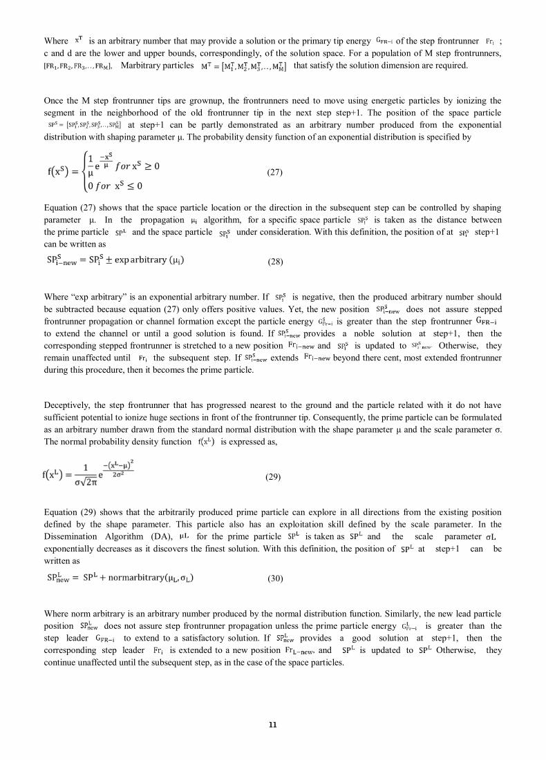
Once the M step frontrunner tips are grownup, the frontrunners need to move using energetic particles by ionizing the
segment in the neighborhood of the old frontrunner tip in the next step step+1. The position of the space particle
at step+1 can be partly demonstrated as an arbitrary number produced from the exponential
distribution with shaping parameter μ. The probability density function of an exponential distribution is specified by
(27)
Equation (27) shows that the space particle location or the direction in the subsequent step can be controlled by shaping
parameter μ. In the propagation algorithm, for a specific space particle is taken as the distance between
the prime particle and the space particle under consideration. With this definition, the position of at step+1
can be written as
(28)
Where “exp arbitrary” is an exponential arbitrary number. If is negative, then the produced arbitrary number should
be subtracted because equation (27) only offers positive values. Yet, the new position does not assure stepped
frontrunner propagation or channel formation except the particle energy is greater than the step frontrunner
to extend the channel or until a good solution is found. If provides a noble solution at step+1, then the
corresponding stepped frontrunner is stretched to a new position and is updated to Otherwise, they
remain unaffected until the subsequent step. If extends beyond there cent, most extended frontrunner
during this procedure, then it becomes the prime particle.
Deceptively, the step frontrunner that has progressed nearest to the ground and the particle related with it do not have
sufficient potential to ionize huge sections in front of the frontrunner tip. Consequently, the prime particle can be formulated
as an arbitrary number drawn from the standard normal distribution with the shape parameter μ and the scale parameter σ.
The normal probability density function is expressed as,
(29)
Equation (29) shows that the arbitrarily produced prime particle can explore in all directions from the existing position
defined by the shape parameter. This particle also has an exploitation skill defined by the scale parameter. In the
Dissemination Algorithm (DA), for the prime particle is taken as and the scale parameter
exponentially decreases as it discovers the finest solution. With this definition, the position of at step+1 can be
written as
(30)
Where norm arbitrary is an arbitrary number produced by the normal distribution function. Similarly, the new lead particle
position does not assure step frontrunner propagation unless the prime particle energy is greater than the
step leader to extend to a satisfactory solution. If provides a good solution at step+1, then the
corresponding step leader is extended to a new position and is updated to Otherwise, they
continue unaffected until the subsequent step, as in the case of the space particles.

12
Dissemination Algorithm (DA) for solving optimal reactive power dispatch problem
a. Algorithm is set by proclaiming the DA parameters such as channel time, reset iteration, frontrunner tip
energies
b. Step frontrunners are produced arbitrarily
c. Fitness is calculated by using cost function.
d. Frontrunner tip energies are modernized.
e. The finest or poorest step frontrunners are determined.
f. Kinetic energy and particle course is modernized.
g. Space and prime particles are evicted.
h. Bifurcating is checked. If bifurcating occurs, two equal channels are produced at bifurcation point and then the
channel which has low energy is eradicated to uphold the population size.
i. Steps (c) to (h) are repetitive until optimization convergence is achieved.
j. Save and print the final solution
The efficiency of the proposed Dissemination Algorithm (DA) for solving the multi-objective optimal reactive power
dispatch problem (OPRD) is demonstrated by testing it on standard IEEE-30 bus system. The IEEE-30 bus system has 6
generator buses, 24 load buses and 41 transmission lines of which four branches are (6-9), (6-10) , (4-12) and (28-27) - are
with the tap setting transformers. The lower voltage magnitude limits at all buses are 0.95 p.u. and the upper limits are 1.1
for all the PV buses and 1.05 p.u. for all the PQ buses and the reference bus. The simulation results have been presented in
Tables 1, 2, 3, 4 &Table 5 shows the proposed algorithm powerfully reduces the real power losses when compared to other
given algorithms. The optimal values of the control variables along with the minimum loss obtained are given in Table 1.
Corresponding to this control variable setting, it was found that there are no limit violations in any of the state variables.
Table 1.Results of DA – ORPD optimal control variables
5. SIMULATION RESULTS
Control variables Variable setting
V1
V2
V5
V8
V11
V13
T11
T12
T15
T36
1.028
1.026
1.022
1.020
1.000
1.024
1.00
1.00
1.00
1.00
Control variables Variable setting
Qc10
Qc12
Qc15
Qc17
Qc20
Qc23
Qc24
Qc29
Real power loss
SVSM
3 2 3 0 2
3 3 2
4.2564
0.2452

13
Optimal Reactive Power Dispatch problem together with voltage stability constraint problem was handled in this case as a
multi-objective optimization problem where both power loss and maximum voltage stability margin of the system were
optimized simultaneously. Table 2 indicates the optimal values of these control variables. Also it is found that there are no
limit violations of the state variables. It indicates the voltage stability index margin (SVSM) has increased from 0.2452 to
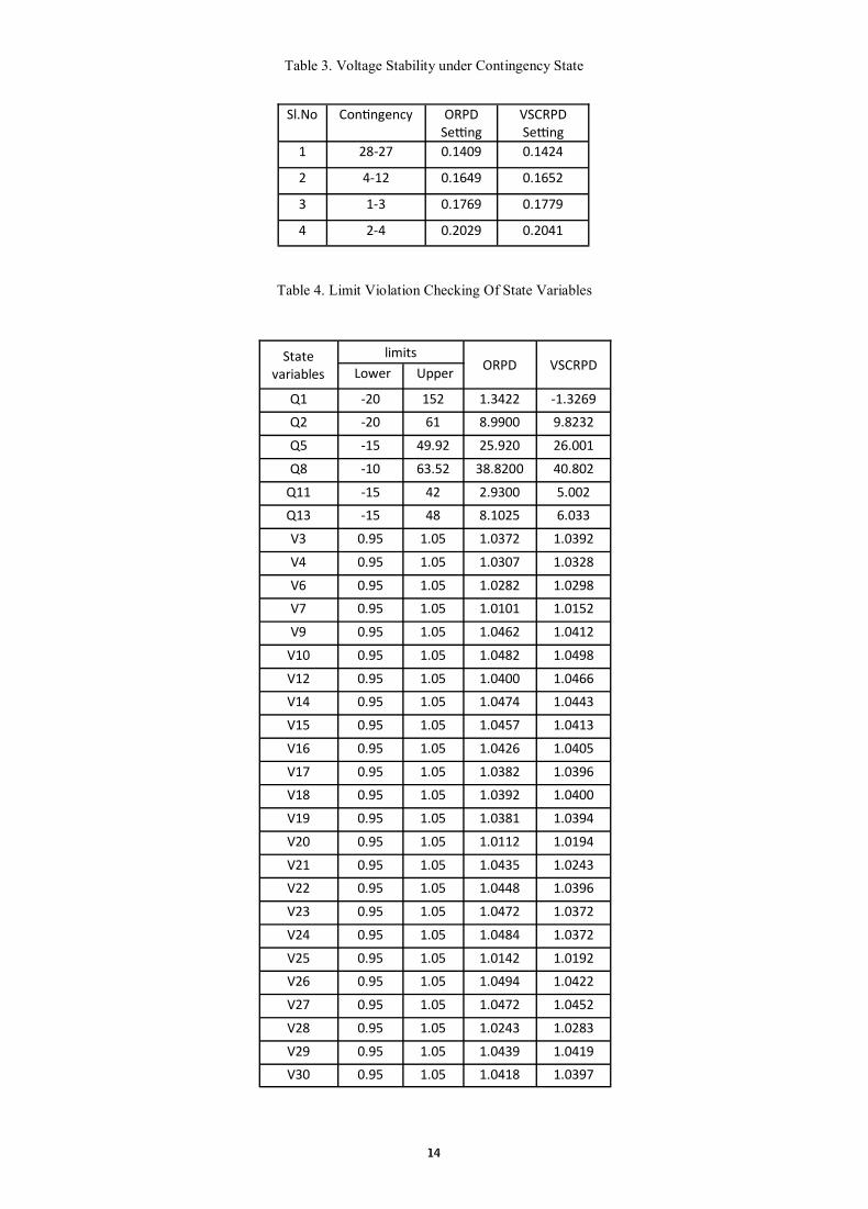
0.2470, an advance in the system voltage stability. To determine the voltage security of the system, contingency analysis
was conducted using the control variable setting obtained in case 1 and case 2. The Eigen values equivalents to the four
critical contingencies are given in Table 3. From this result it is observed that the Eigen value has been improved
considerably for all contingencies in the second case. In Table 4 limit violation checking of State variables is given.
Table 2.Results of DA -Voltage Stability Control Reactive Power Dispatch Optimal Control Variables
Control Variables Variable Setting
V1
V2
V5
V8
V11
V13
T11
T12
T15
T36
Qc10
Qc12
Qc15
Qc17
Qc20
Qc23
Qc24
Qc29
Real power loss
SVSM
1.030
1.032
1.036
1.029
1.000
1.027
0.090
0.090
0.090
0.090 3 3 2 3 0 2 2 3
4.9868
0.2470
14
Table 3. Voltage Stability under Contingency State
Table 4. Limit Violation Checking Of State Variables
Sl.No Contingency ORPD Setting
VSCRPD Setting
1 28-27 0.1409 0.1424
2 4-12 0.1649 0.1652
3 1-3 0.1769 0.1779
4 2-4 0.2029 0.2041
State variables
limits ORPD VSCRPD
Lower Upper
Q1 -20 152 1.3422 -1.3269
Q2 -20 61 8.9900 9.8232
Q5 -15 49.92 25.920 26.001
Q8 -10 63.52 38.8200 40.802
Q11 -15 42 2.9300 5.002
Q13 -15 48 8.1025 6.033
V3 0.95 1.05 1.0372 1.0392
V4 0.95 1.05 1.0307 1.0328
V6 0.95 1.05 1.0282 1.0298
V7 0.95 1.05 1.0101 1.0152
V9 0.95 1.05 1.0462 1.0412
V10 0.95 1.05 1.0482 1.0498
V12 0.95 1.05 1.0400 1.0466
V14 0.95 1.05 1.0474 1.0443
V15 0.95 1.05 1.0457 1.0413
V16 0.95 1.05 1.0426 1.0405
V17 0.95 1.05 1.0382 1.0396
V18 0.95 1.05 1.0392 1.0400
V19 0.95 1.05 1.0381 1.0394
V20 0.95 1.05 1.0112 1.0194
V21 0.95 1.05 1.0435 1.0243
V22 0.95 1.05 1.0448 1.0396
V23 0.95 1.05 1.0472 1.0372
V24 0.95 1.05 1.0484 1.0372
V25 0.95 1.05 1.0142 1.0192
V26 0.95 1.05 1.0494 1.0422
V27 0.95 1.05 1.0472 1.0452
V28 0.95 1.05 1.0243 1.0283
V29 0.95 1.05 1.0439 1.0419
V30 0.95 1.05 1.0418 1.0397

15
Table 5. Comparison of Real Power Loss
In this paper, Dissemination Algorithm (DA) has been successfully solved Optimal Reactive Power Dispatch problem.
Proposed Dissemination Algorithm (DA) based on natural phenomenon of lightning and the process based on theory of fast
particles. To distinguish the transition particles that produce the first step frontrunner population, three particle kinds are
established & the space particles that attempt to turn out to be the frontrunner, the key particle that exemplify the particle
excited from most excellent located step frontrunner. The proposed Dissemination Algorithm (DA) has been tested in
standard IEEE 30, bus test system and simulation results show clearly about the improved performance of the projected
Dissemination Algorithm (DA) in reducing the real power loss and static voltage stability margin (SVSM) has been
enhanced.
1. O.Alsac, and B. Scott, “Optimal load flow with steady state security”,IEEE Transaction. PAS -1973, pp. 745-751.
2. Lee K Y ,Paru Y M , Oritz J L –A united approach to optimal real and reactive power dispatch , IEEE Transactions on power Apparatus and systems 1985: PAS-104 : 1147-1153
3. A.Monticelli , M .V.F Pereira ,and S. Granville , “Security constrained optimal power flow with post contingency corrective rescheduling” , IEEE Transactions on Power Systems :PWRS-2, No. 1, pp.175-182.,1987.
4. Deeb N, Shahidehpur S.M ,Linear reactive power optimization in a large power network using the decomposition approach. IEEE Transactions on power system 1990: 5(2) : 428-435
5. E. Hobson ,’Network consrained reactive power control using linear programming, ‘ IEEE Transactions on power systems PAS -99 (4) ,pp 868=877, 1980
6. K.Y Lee ,Y.M Park , and J.L Oritz, “Fuel –cost optimization for both real and reactive power dispatches” , IEE Proc; 131C,(3), pp.85-93.
7. M.K. Mangoli, and K.Y. Lee, “Optimal real and reactive power control using linear programming” , Electr.Power Syst.Res, Vol.26, pp.1-10,1993.
8. C.A. Canizares , A.C.Z.de Souza and V.H. Quintana , “ Comparison of performance indices for detection of proximity to voltage collapse ,’’ vol. 11. no.3 , pp.1441-1450, Aug 1996 .
9. K.Anburaja, “Optimal power flow using refined genetic algorithm”, Electr.Power Compon.Syst , Vol. 30, 1055-1063,2002.
10. D. Devaraj, and B. Yeganarayana, “Genetic algorithm based optimal power flow for security enhancement”, IEE proc-Generation.Transmission and. Distribution; 152, 6 November 2005.
11. A. Berizzi, C. Bovo, M. Merlo, and M. Delfanti, “A ga approach to compare orpf objective functions including secondary voltage regulation,” Electric Power Systems Research, vol. 84, no. 1, pp. 187 – 194, 2012.
12. C.-F. Yang, G. G. Lai, C.-H. Lee, C.-T. Su, and G. W. Chang, “Optimal setting of reactive compensation devices with an improved voltage stability index for voltage stability enhancement,” International Journal of Electrical Power and Energy Systems, vol. 37, no. 1, pp. 50 – 57, 2012.
Method Minimum loss (MW)
Evolutionary programming [23] 5.0159
Genetic algorithm [24] 4.665
Real coded GA with Lindex as SVSM [25]
4.568
Real coded genetic algorithm [26] 4.5015
Proposed AA method 4.2564
6. CONCLUSION
REFERENCES

16
13. P. Roy, S. Ghoshal, and S. Thakur, “Optimal var control for improvements in voltage profiles and for real power loss minimization using biogeography based optimization,” International Journal of Electrical Power and Energy Systems, vol. 43, no. 1, pp. 830 – 838, 2012.
14. B. Venkatesh, G. Sadasivam, and M. Khan, “A new optimal reactive power scheduling method for loss minimization and voltage stability margin maximization using successive multi-objective fuzzy lp technique,” IEEE Transactions on Power Systems, vol. 15, no. 2, pp. 844 – 851, may 2000.
15. W. Yan, S. Lu, and D. Yu, “A novel optimal reactive power dispatch method based on an improved hybrid evolutionary programming technique,” IEEE Transactions on Power Systems, vol. 19, no. 2, pp. 913 – 918, may 2004.
16. W. Yan, F. Liu, C. Chung, and K. Wong, “A hybrid genetic algorithminterior point method for optimal reactive power flow,” IEEE Transactions on Power Systems, vol. 21, no. 3, pp. 1163 –1169, aug. 2006.
17. J. Yu, W. Yan, W. Li, C. Chung, and K. Wong, “An unfixed piecewiseoptimal reactive power-flow model and its algorithm for ac-dc systems,” IEEE Transactions on Power Systems, vol. 23, no. 1, pp. 170 –176, feb. 2008.
18. F. Capitanescu, “Assessing reactive power reserves with respect to operating constraints and voltage stability,” IEEE Transactions on Power Systems, vol. 26, no. 4, pp. 2224–2234, nov. 2011.
19. Z. Hu, X. Wang, and G. Taylor, “Stochastic optimal reactive power dispatch: Formulation and solution method,” International Journal of Electrical Power and Energy Systems, vol. 32, no. 6, pp. 615 – 621, 2010.
20. A. Kargarian, M. Raoofat, and M. Mohammadi, “Probabilistic reactive power procurement in hybrid electricity markets with uncertain loads,” Electric Power Systems Research, vol. 82, no. 1, pp. 68 – 80, 2012.
21. Berkopec .A (2012), “Fast Particles as Initiators of Stepped Leaders in CG and IC Lightnings,” Journal of Electrostat, vol.70, pp. 462–467.
22. Tizhoosh.H.R (2005) “Opposition-Based Learning: A New Scheme for Machine Intelligence,” CIMCA/IAWTIC. pp. 695–701.
23. Wu Q H, Ma J T. “Power system optimal reactive power dispatch using evolutionary programming”, IEEE Transactions on power systems 1995; 10(3): 1243-1248 .
24. S.Durairaj, D.Devaraj, P.S.Kannan, “Genetic algorithm applications to optimal reactive power dispatch with voltage stability enhancement”, IE(I) Journal-EL Vol 87,September 2006.
25. D.Devaraj, “Improved genetic algorithm for multi – objective reactive power dispatch problem”, European Transactions on electrical power 2007; 17: 569-581.
26. P. Aruna Jeyanthy and Dr. D. Devaraj “Optimal Reactive Power Dispatch for Voltage Stability Enhancement Using Real Coded Genetic Algorithm”, International Journal of Computer and Electrical Engineering, Vol. 2, No. 4, August, 2010 1793-8163.

17
PERFORMANCE AND COST ANALYSIS OF BIO- DIESEL PRODUCTION FROM MILLETIA
PINNATTA
Adarsh S Faculty of Civil Engineering Department
Vidya Vikas Institute of Engineering and Technology
Bannur Road, Alanahally, Mysuru-570028, Karnataka, India
9538438191, [email protected]
Anusha M Faculty of Civil Engineering Department
Vidya Vikas Institute of Engineering and Technology
Bannur Road, Alanahally, Mysuru-570028, Karnataka, India
9986879811, [email protected]
Shesha Prakash M N* Vice Principal, Professor and Head of Civil Engineering Department
Vidya Vikas Institute of Engineering and Technology
Bannur Road, Alanahally, Mysuru-570028, Karnataka, India
9740011400, [email protected]
*Corresponding author
Biodiesel has become a key source as a substitute fuel and is rightly getting its significance as a key future renewable
energy source. As an alternative fuel for diesel engines, it is becoming increasingly important due to diminishing
petroleum reserves and the environmental consequences of exhaust gases from petroleum-fuelled engines. Further it also
helps in countries economy as it depends on reserve financial exchange.
Biodiesel is an alternative to conventional diesel fuel made from renewable resources, such as non-edible vegetable oils.
The oil from seeds (e.g., Jatropha, Milletia Pinnatta etc) can be converted to a fuel commonly referred to as "Biodiesel". In
this research work, the seed Milletia Pinnatta is being used to extract the biodiesel. No engine modifications are required to
use biodiesel in place of petroleum-based diesel. Biodiesel can be mixed with petroleum-based diesel in any proportion. The
use of biodiesel resulted in lower emissions of unburned hydrocarbons, carbon monoxide, and particulate matter. The fuel
consumption in the world particularly in developing countries has been growing at alarming rate. Petroleum prices
approaching record highs and depleting source within few years, it is clear that more focus can be done to utilize domestic
non-edible oils while enhancing our energy security. The economic benefits include support to the agriculture sector,
tremendous employment opportunities in plantation and processing. This paper reviews the Cost and performance analysis
of Bio-Diesel using the seed Millettia Pinnata and estimate Calorific Value and Viscosity of Bio-Diesel.
Key words: Milletia Pinnatta, Bio-Diesel, Transesterification, Blending, Calorific value.
ABSTRACT

18
With the increasing use of diesel fuel, many initiatives have become more attractive to search for alternate fuels to supply or
replace fossil fuels. Biodiesel is synthesized from edible, non-edible and waste cooking oil or animal oil can be regarded as
an alternative diesel fuel. The various alternative fuel options tried in place of hydrocarbon oils are mainly biogas, producer
gas, ethanol, methanol and vegetable oils. Out of all these, biodiesel offers an advantage because of their comparable fuel
properties with that of diesel. The emissions produced from biodiesel are cleaner compared to petroleum-based diesel fuel.
Particulate emissions, soot, and carbon monoxide are lower since biodiesel is an oxygenated fuel. The biodiesel could be
used as pure fuel or as blend with petro diesel, which is stable with all ratios. Alternative new and renewable fuels have the
potential to solve many of the current social problems and concerns, from air pollution and global warming to other
environmental improvements and sustainability issues (Deepak Verma et.al.2016).
Biodiesel is defined as monoalkyl esters of long chain fatty acids originated from natural oils and fats of plants
and animals, is a kind of alternative for fossil fuels. Biodiesel has attracted wide attention in the world due to its
renewability, biodegradability, nontoxicity and environmental friendly benefits (Alemayehu Gashaw et.al. 2015). Fuels
derived from green source for use in diesel engines are known as biodiesel. Biodiesel consists of the methyl ester of the
fatty acid component of the triglyceride. (Md. Atiqur Rahman et.al. 2016).
Biodiesel has higher oxygen content than petroleum diesel and its use in diesel engines have shown great reductions in
emission of particulate matter, carbon monoxide, sulfur, polyaromatics, hydrocarbons, smoke and noise. In addition,
burning of vegetable-oil based fuel relatively contributes lesser towards carbon footprint because such fuel is made from
agricultural materials which are produced via photosynthetic carbon fixation (Tanarkorn Sukjit et.al.2013).
The only advantage of biofuels is their carbon content and the little amount of carbon waste they expel into the air after they
are used when compared with that of fossil fuel. (Ogunwole O.A, 2012).|
For biodiesel to be considered as a sustainable source of energy, the input of energy into the extraction or production of
biodiesel must not exceed the output of the energy that can be extracted from the biodiesel. Sustainable energy can be
achieved through extensive research on energy involved in biodiesel production. That is, improvement on energy efficiency
of biodiesel production will reduce biodiesel production cost and make life more bearable to man. (Ayoola A.A.et.al.2016).
There are various processes which can be applied to synthesize biodiesel such as direct use and blending, micro emulsion
process, thermal cracking process and among this, the most conventional way is transesterification process. This is
because of the fact that this method is relatively easy, carried out at normal conditions, and gives the best conversion
efficiency and quality of the converted fuel (Alemayehu Gashaw et.al. 2015).
2.1 Transesterification (Alcoholysis)
Transesterification, refers to a catalyzed chemical reaction involving vegetable oil and an alcohol to yield fatty acid alky
esters (i.e., biodiesel) and glycerol (M. Thirumarimurugan et.al. 2012).
Transesterification is a chemical reaction used for the conversion of seed oil to bio diesel. In this process seed oil is
chemically reacted with an alcohol like methanol or ethanol in presence of catalyst like KOH or NaOH. Transesterification
of seed oil is the most popular method of producing biodiesel. Transesterification (alternatively alcoholysis) is the reaction
of a fat or oil (trigylceride) with an alcohol to form fatty acid alkyl esters (valuable intermediates in oleo chemistry), methyl
and ethyl esters (which are excellent substitutes for biodiesel) and glycerol as shown:
1. INTRODUCTION
2. PRODUCTION OF BIODIESEL
19
Transesterification as an industrial process is usually carried out by heating an excess of the alcohol with seed oil under
different reaction conditions in the presence of an inorganic catalyst. The reaction is reversible and therefore excess alcohol
is used to shift the equilibrium to the products side. The alcohols that can be used in the transesterification process are
methanol, ethanol, propanol, butanol and amyl alcohol, with methanol and alcohol being frequently used. The reactions are
often catalysed by an acid, a base or enzyme to improve the reaction rate and yield. Thus during this process nothing is
wasted. All the products and by-products are utilized for various purposes. (Wilson Parawira, 2010).
2.2 Direct Use and Blending
The direct use of seed oil in diesel engine is not favorable and problematic because it has many inherent failings. Even
though the seed oil have familiar properties as biodiesel fuel, it required some chemical modification before can be used
into the engine (Alemayehu Gashaw et.al. 2015).
Biodiesel fuel is presently attracting increasing attention worldwide as a blending component or a direct replacement for
diesel fuel in vehicle engines. When blended with diesel fuel the designation BXX indicates the XX% amount of biodiesel
in the blend, for example B30 is 30% biodiesel and 70% diesel. It has been reported that blends up to B20 can be used in
nearly all diesel equipment and are compatible with most storage and distribution equipment. These low-level blends
generally do not require any engine modifications. However, higher blends or B100 can be used in many engines built with
little or no modification (Aransiola EF et.al.2012).
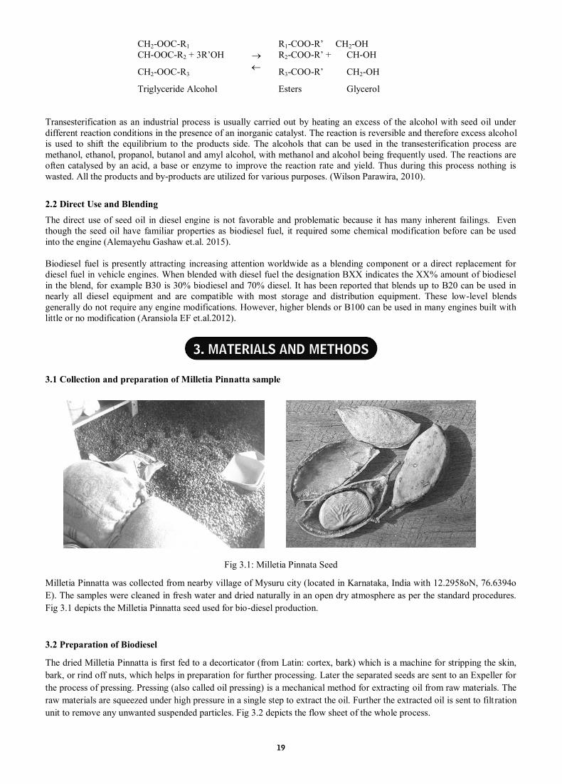
3.1 Collection and preparation of Milletia Pinnatta sample
Fig 3.1: Milletia Pinnata Seed
Milletia Pinnatta was collected from nearby village of Mysuru city (located in Karnataka, India with 12.2958oN, 76.6394o
E). The samples were cleaned in fresh water and dried naturally in an open dry atmosphere as per the standard procedures.
Fig 3.1 depicts the Milletia Pinnatta seed used for bio-diesel production.
3.2 Preparation of Biodiesel
The dried Milletia Pinnatta is first fed to a decorticator (from Latin: cortex, bark) which is a machine for stripping the skin,
bark, or rind off nuts, which helps in preparation for further processing. Later the separated seeds are sent to an Expeller for
the process of pressing. Pressing (also called oil pressing) is a mechanical method for extracting oil from raw materials. The
raw materials are squeezed under high pressure in a single step to extract the oil. Further the extracted oil is sent to filtration
unit to remove any unwanted suspended particles. Fig 3.2 depicts the flow sheet of the whole process.
CH2-OOC-R1 R1-COO-R’ CH2-OH CH-OOC-R2 + 3R’OH
R2-COO-R’ + CH-OH
CH2-OOC-R3 R3-COO-R’ CH2-OH
Triglyceride Alcohol Esters Glycerol
3. MATERIALS AND METHODS

20
3.3 Transesterification of Single Stage Process
Transesterification is a chemical reaction used for the conversion of seed oil to bio diesel. In this process seed oil is
chemically reacted with an alcohol like methanol or ethanol in presence of catalyst like KOH or NaOH. After the chemical
reaction various components of seed oil breaks down to form new compounds. The triglycerides are converted into alkyl
esters, which is the chemical name of bio diesel. If methanol is used in the chemical reaction, methyl esters are formed, but
if ethanol is used, then ethyl esters are formed. Both these compounds are bio diesel fuels with different chemical
combinations. In this chemical reaction alcohol replaces glycerine. Glycerine that has been separated during the
transesterification process is released as a bi product of the chemical reaction. Glycerine will either sink to the bottom of the
reaction vessel or come to the surface depending on its phase. It can be easily separated by centrifuges, and this entire
process is known as transesterification. The by-product of transesterification chemical reaction is the glycerine that
originally formed the bond between the chains of fatty acids. Table 3.1 gives the outlook of the Apparatus, Equipments,
Chemicals and Raw material used in transesterification process.
Fig 3.2:Flow Chart of Bio-diesel preparation Process.
Table 3.1: Requirements for Transesterification Process.
Blending
Extracted biodiesel are mixed with the regular diesel for different blends B30, B35, B40 (shown in Table 3.2) and the
blended biodiesel is checked for different parametric tests like density, viscosity and calorific values.
Table 3.2: Blends Ratio per Litre
Collection of Milletia Pinna-
ta Seed
Decorticator
Expeller
Oil Filter
transesterification
unit
Apparatus Equipments Chemicals Raw material
3 neck flask (2000ml ) Test tube Standard flask (1000ml ) Glass rod Heater with magnetic stirrer Reflux Burette (50ml)
Decorticator Expeller Oil Filter Transesterification unit
Methanol Sodium Hydroxide (NaOH) Isotrophyl alcohol (C3H7OH)
Milletia Pinnatta
seed
Blends B30 B35 B40
Diesel (ml) 700 650 600 Biodiesel (ml) 300 350 400

21
i. Measurement of Density of Biodiesel
Biodiesel of different blends are obtained as per the requirements by blending biodiesel with the normal diesel
of different proportions. Different blends are collected in different measuring jars of about 0.5L each. A
hydrometer is introduced into the measuring jar filled with biodiesel-blends to know the density which starts
floating. The reading obtained in the hydrometer is recorded.
ii. Measurement of Viscosity of Biodiesel
The apparatus is cleaned thoroughly and water jacket is filled with water. The gate orifice is closed using the
iron ball which acts as a valve. The oil cup is filled with 50cc of the given lubricating oil. Two thermometers
for measuring the water and soil temperatures are introduced to the respective slots in the apparatus at the
room temperature. The ball valve is opened and allowed to flow through the standard orifice. The weight of
the oil collected is noted and oil is poured back into the cup. The specific gravity of the oil is calculated. Now
the apparatus is electrically heated. At any particular temperature, the ball valve is opened and oil is allowed to
flow through the standard orifice. Time for the 50cc of oil to flow through orifice is noted. The time in second
is called as Red woods seconds, is noted down.
iii. Measurement of Calorific Value of Biodiesel
Exactly 1cc of the fuel i.e. Biodiesel oil corresponding to 0.8 gins of fuel is taken. The fuel is poured into brass
crucible and the crucible is placed inside the bomb calorimeter. The fuse wire is inserted into the crucible so
that it is completely dipped in the fuel and then the bomb calorimeter is filled with oxygen to a pressure of
2MPa. A sensitive thermometer (sensitivity 0.5ºC) is placed in its slot in the water jacket. The pressurized
bomb calorimeter is placed inside the jacket and the water is stirred (until the experiment concludes) at
intervals of 30 seconds and the corresponding temperature is recorded. The bomb calorimeter is ignited by
switching on and switching off simultaneously. The temperature starts to increase because of combustion and
at intervals of 30 seconds and the corresponding temperatures are recorded until the maximum temperature.
Then the temperature starts to decrease and again the temperatures are recorded at 30 second intervals, the
above measurements are necessary to account for radiation losses if any.
Since biodiesel is produced from Milletia Pinnatta seed, the pure biodiesel must meet before being used as a pure
fuel or being blended with conventional diesel fuels. Various parameters which define the quality of biodiesel are
discussed below.
As discussed earlier in the methodology, Extracted biodiesel are mixed with the regular diesel for different blends B30,
B35, B40 and the blended biodiesel is checked for different parametric tests like density, viscosity, calorific values and
flash point as shown in table 4.1. The viscosity of a liquid is a measure of its resistance to flow due to internal
friction; this is a very important property of a diesel fuel because it affects the engine fuel injection system
predominantly at low temperatures, it can be seen that the viscosity value obtained is 0.38 , 0.39 and 0.41 stokes
respectively for 3 blends which has achieved medium viscosity level which does not generates operational problems like
difficulty in engine starting, unreliable ignition and deterioration in thermal efficiency. The density of diesel fuels is another
important property of the fuels that affects the fuel injection system. Density of biodiesel is the weight of a unit volume of
fluid while the specific gravity is the ratio of the density of a liquid to the density of water. The fuel injection equipment
meters the fuel volumetrically and high densities translate into a high consumption of the fuel. It can be seen that biodiese l
has densities between 835 kg/m3 to 860 kg/m3 which is again within the acceptable range where we can expect low
consumption of fuel with more efficiency. The biodiesel sample has achieved a good calorific value of 8796, 6330 and 3061
kcal/kg for 3 different blends. The biodiesel sample has a higher flash point of about 150oC as compared to the standard
diesel flash point of about 50 0C. This makes the biodiesel sample safe for use and storage. Fuels with lower flash point
which tend to ignite at lower temperatures making them highly dangerous if not stored and used properly.
Table 4.1 Biodiesel properties obtained from Milletia Pinnatta seed
4. RESULTS AND DISCUSSION
Sr. No Blends Kinematic viscosity
(stokes) Density
(kg/m3) CalorificValues
(KCal/Kg) Flash point
(0C)
1 B 30 0.38 835 8796 150
2 B 35 0.39 850 6330 150
3 B 40 0.41 860 3061 150
4 Standard
( ASTM D 6751) 0.02-0.5 800-900 1000-9500 100-170

22
4.1 Emission Analysis
Emission analysis which is considered as one of the major part of the research work was conducted for normal diesel, as
well as for different blended bio-diesel. The vehicle used for emission test was TATA Indica Vista (2005 Model) diesel
engine, Vehicle Registration Number – KA-05 MF-9413 as shown in Fig 4.1, emission analysis results is as shown in table
4.2 and the respective emission analysis comparison graph for normal diesel and different blended bio-diesel is as shown in
Fig 4.2.
Fig 4.1: Vehicle Used for Emission Analysis.
Table 4.2: Emission analysis Values for Regular Diesel
*HSU- Horton’s Smoke unit.
Fig 4.2: Emission Analysis Comparison Graph for Normal Diesel and Different Blended Bio-Diesel.
4.2 Performance Analysis
In order to conduct a performance analysis a total quantity of 5 liters of biodiesel blend was added to the diesel engine and
then the performance was analyzed per liter of biodiesel blends added. The performance analysis is done for blended diesel
and normal diesel which gave a average mileage of 18.6 Kmpl for blended biodiesel and 18 Kmpl for normal diesel which
proves to be biodiesel is more efficient than normal diesel, results are as shown in table 4.3, and the respective performance
analysis comparison between normal diesel and different blended bio-diesel is as shown in table 4.4. The respective
Emission
Analysis
Values for
Regular Diesel B30 B35 B40
Sl.No 1 2 3 Mean 1 2 3 Mean 1 2 3 Mean 1 2 3 Mean
RPM Min 1881 1519 1960 1871 1500 1950 1860 1480 1935 1855 1470 1930
RPM Max 3750 3429 3371 3730 3416 3355 3722 3405 3333 3715 3400 3325
Km 0.28 0.27 0.27 0.27 0.27 0.27 0.26 0.27 0.26 0.26 0.26 0.26 0.26 0.25 0.25 0.25
HSU% 11.4 11.2 11.2 11.2 11.2 11.1 11.1 11.1 11.08 11.07 11.07 11.07 11.07 11.05 11.05 11.05

23
performance analysis comparison graph for normal diesel and different blended bio-diesel is as shown in Fig 4.3.
Table 4.3: Performance analysis Values for B30, B35, B40.
Table 4.4: Performance analysis Comparison between Normal Diesel and Different Blends
Fig 4.3 Performance Analysis Comparison Graph for Normal Diesel and Different Blended Bio-Diesel.
4.3 Cost Analysis
Cost analysis which is the main objective of the research work is done and compared with the normal diesel rate which is
Rs.63.00 dated as on 27/02/2018 which seems to be more than the blended bio-diesel which costs Rs.38.71 for B30,
Rs.38.45 for B35 and Rs.38.20 for B40 respectively. Cost analysis results is as shown in table 4.5 and the respective cost
analysis comparison graph for normal diesel and different blended bio-diesel is as shown in Fig 4.4.
Table 4.5: Cost Analysis between Blended Bio-Diesel and Normal Diesel
Biodiesel blend
Quantity of Biodiesel (Lts)
Initial odometer reading (Kms)
Final odometer reading (Kms)
Total distance travelled (Kms)
Average Mileage (Kmpl)
B30 5 60187 60278 91 18.2
B35 5 60278 60371 93 18.6
B40 5 60371 60464 93 18.6
Blends Efficiency for Biodiesel
Blends (Kmpl)
Normal Diesel 18.0
B30 18.2
B35 18.6
B40 18.6
Blends Cost for Blends
(Rupees)
Normal Diesel 63.00
B30 38.71
B35 38.45
B40 38.20

24
Fig 4.4: Cost Analysis Comparison Graph for Normal Diesel and Different Blended Bio-Diesel.
The biodiesel produced by the process of transesterification has relatively much lower viscosity. The calorific value
decreases as the blends increase. Hence, amount of heat produced by the biodiesel decreases as the blends increase which
ensures the safety of the engine from catching fire. The viscosity and the density of biodiesel increase as the blends
increase.
The cost of the biodiesel extracted by Milletia pinnatta seed is much lower than the cost of the petroleum diesel and hence
the biodiesel is economical fuel to operate diesel engines. The efficiency of the diesel engine run by petroleum diesel is
lesser than the efficiency of the diesel engine that is run by biodiesel fuel. Hence biodiesel is most economical and efficient
fuel to run the diesel engines. This makes it capable of replacing petroleum diesel in diesel engines to make the world more
eco-friendly and sustainable.
1. Alemayehu Gashaw, Tewodros Getachew and AbileTeshita (2015) A Review on Biodiesel Production as
Alternative Fuel, 4(2): 80-85
2. Alemayehu Gashaw and Amanu Lakachew (2014) Production of Biodiesel From Non Edible Oil and its Properties.
International Journal of Science, Environment and Technology, 3(4), 1544 – 1562.
3. Aransiola, E. F, Betiku, E. Ikhuomoregbe, D.I.O., Ojumu T.V. (2012) Production of biodiesel from crude neem oil
feedstock and its emissions from internal combustion engines. African Journal of Biotechnology, 11(22): 6178-
6186.
4. Ayoola A.A., Oresegun O.R., Oladimeji T.E., Eneghalu (2016) Energy Analysis of Biodiesel Production from
Waste Groundnut Oil. International Journal of Research in Engineering and Applied Sciences, PP 2249-3905.
5. Deepak Verma, Janmit Raj, Amit Pal, Manish Jain (2016) A critical review on production of biodiesel from various
feed stocks. Journal of Scientific and Innovative Research, 5(2): 51-58.
6. Md. Atiqur Rahman & Kamrun Nahar (2016) Production and Characterization of Algal Biodiesel from Spirulina
Maxima. Global Journal of Researches in Engineering, PP 2249-4596.
7. Ogunwole, O.A. (2012) Production of Biodiesel from Jatropha Oil (Curcas Oil), Research Journal of Chemical
Sciences, 2(11), 30-33.
8. Parawira, W. (2010) Biodiesel production from Jatrophacurcas: A review. Scientific Research and Essays, 5(14),
1796-1808.
9. Sukjit,T., Punsuvon, V. (2013) Process Optimization of Crude Palm Oil Biodiesel Production by Response Surface
Methodology. European International Journal of Science and Technology, 2(7)49-56.
10. Thirumarimurugan, M., Sivakumar, V. M., Merly Xavier, A., Prabhakaran, D.,Kannadasan, T. (2012) Preparation of
Biodiesel from Sunflower Oil by Transesterification, International Journal of Bioscience, Biochemistry and
Bioinformatics, 2(6), 441-444.
5. CONCLUSION
REFERENCES

25
DESIGN & IMPLEMENTATION OF REGENERATIVE BRAKING AND LOAD EQUALISATION USING
PMDC MOTOR
Mahesh K Professor EEE
New Horizon College of Engineering,
Bangalore-560103
Mobile: 09900119252
Lithesh J* New Horizon College of Engineering,
Bangalore-560103
Mobile: 9164609997
* Corresponding author
Sriguru A Sajjan New Horizon College of Engineering,
Bangalore-560103
Mobile: 8088401964
There are several advantage of using Permanent Magnet DC motor (PMDC), where the drive can work in all four quadrants.
Out of these four quadrants, two quadrants are motoring and other two are braking. During motoring the power is consumed
by the motor and during braking the power is given back to the source. This power which is given back to the source during
braking is regenerative braking. In this paper, the Hardware Implementation of Regenerative Braking and Load
Equalization is carried out using the PMDC Motor. The importance of the PMDC motor is elaborated due to its high
efficiency and wide usage in the market (BEV- Battery Electric Vehicles). The drives take large current when the load
torque is high and hence there will be a dip in voltage of the source due to this load torque. Hence this affects the other
loads connected to the same source. Through Load Equalization, the flywheel is connected to the motor shaft so that the
flywheel can give enough load torque during high torque period. During light load period, the power can be given back to
the source through Regenerative Braking. To gain kinetic energy of the motor in the form of inertia, the supply is cut off so
as to achieve Regenerative Braking with the help of a flywheel.
Keywords: flywheel, load equalization, four quadrant operation, regenerative braking.
ABSTRACT

26
Regenerative braking, load equalization, four quadrant operation are some of the important concepts in Electrical Drives.
There are several loads which has a capability of driving the motor due to the movement of the load due to stored kinetic
energy that is in the form of inertia, this energy can be harnessed and fed back to the source hence saving electricity which
gives rise to regenerative braking. Similarly many loads are fluctuating in nature, where the load needs maximum energy
from the motor for very short time, and the load requires very minimum energy just to compensate the losses. Hence the
motor consumes very high power from the source for short time followed by very less power for some time, and this cycle
repeats. But the motor cannot be chosen according to the maximum load torque demanded by load for short time, as it is not
economical. Moreover the motor will draw very high current due to high load torque, this causes dip in the source voltage
and affects other loads connected to the same source. This problem can be eliminated by attaching a flywheel to the motor
shaft. This process is called Load Equalization.[5]
PMDC MOTOR
PMDC motor is used in the regenerative braking as PMDC motor can also act as generator and operate in the all the four
quadrants of DC drives. An alternator used in present automobiles generate electricity only when the vehicle is moving,
where by the use of PMDC motor, the electricity can be generated even during at the time of braking hence regenerative
braking can be achieved.
REGENERATIVE BRAKING
In Regenerative Braking, the power or energy of the driven machinery which is in kinetic form is returned back to the
power supply mains. Under this condition, the back emf Eb of the motor is greater than the supply voltage V, which
reverses the direction of motor armature current. The machine now begins to operate as a generator and the energy
generated is supplied to the source.[1][4][5]
LOAD EQUALIZATION
Load equalisation is the process of smoothing the fluctuating load. The fluctuate load draws heavy current from the supply
during the peak interval and also cause a large voltage drop in the system due to which the equipment may get damage.
Load equalisation is achieved with the help of flywheel, flywheel stores energy during light load and utilizes it when the
peak load occurs. Thus, the electrical power from the supply remains constant, hence protecting the appliances which are all
connected to the same source.[5]
Fig 1:Block Diagram
1. INTRODUCTION
2. BLOCK DIAGRAM OF THE EXPERIMENT

27
Components of the block diagram are as shown in Fig 1:
1. Source
2. H Bridge (Manual operation)
3. Permanent magnet D.C motor (1HP, 24V, 38A, 1500 rpm)
4. Rotational load (Flywheel 22.9cm diameter, 12kg)
Source The source is for the PMDC motor, the source is nothing but D.C supply. Here the D.C supply (up to 24V) is generated
from the D.C motor-generator set. However, Digital meters used to measure the regenerated voltage and current at the load
side is fed from auxiliary A.C supply (240V)
The supply voltage (up to 24V) to the motor is generated by the motor generated set, Analog voltmeter is connected in
parallel and analogue ammeter is connected in series in the supply side, to measure the supply voltage and current
respectively.
Fig 2:Source ( DC voltage upto 24V is generated from DC motor-generator set)
PMDC MOTOR
Fig 3:PMDC motor (1HP, 24V, 38A, 1500 rpm)
In permanent magnet dc motors, field excitation is obtained by suitably mounting permanent magnets on the stator. Ferrites
or rare earth (cobalt samarium) magnets are employed. Ferrites are commonly used because of lower cost, but the machine
becomes bulky due to low retentivity. Rare earths because of their high retentivity allow a large reduction in weight and
size, but they are very expensive. Use of permanent magnets for excitation eliminates field copper loss and need for field
supply. In a PMDC motor, permanent magnets (located in stator) provide magnetic field, instead of stator winding.
The stator is usually made from steel in cylindrical form. Permanent magnets are usually made from rare earth materials. The rotor is slotted armature which carries armature
winding. Rotor is made from layers of laminated silicon steel to reduce eddy current losses. Ends of armature winding are

28
connected to commutator segments on which the brushes rest. Commutator is made from copper and brushes are usually
made from carbon or graphite. DC supply is applied across these brushes. The commutator is in segmented form to achieve
unidirectional torque. The reversal of direction can be easily achieved by reversing polarity of the applied voltage.
PRINCIPLE OF OPERATION OF PMDC MOTOR
The working principle of PMDC motor is just similar to the general working principle of DC motor. That is when a carrying
conductor comes inside a magnetic field, a mechanical force will be experienced by the conductor and the direction of this
force is governed by Fleming’s left hand rule. As in a permanent magnet DC motor, the armature is placed inside the
magnetic field of permanent magnet; the armature rotates in the direction of the generated force. Here each conductor of the
armature experiences the mechanical force F = B.I.L Newton where, B is the magnetic field strength in Tesla (weber / m2),
I is the current in Ampere flowing through that conductor and L is length of the conductor in metre comes under the
magnetic field. Each conductor of the armature experiences a force and the compilation of those forces produces a torque,
which tends to rotate the armature
ROTATIONAL LOAD – FLYWHEEL
A flywheel is a mechanical device specifically designed to efficiently store rotational energy. Flywheels resist changes in
rotational speed by their moment of inertia. The amount of energy stored in a flywheel is proportional to the square of its
rotational speed. Here we are using a flywheel of 22.9cm diameter, 12kg. In our project the main aim of having the flywheel
as a load is for two purposes, the kinetic energy of vehicle lost during braking can be converted to electricity, i.e the
flywheel stores energy when torque is applied by the energy source, and it releases stored energy when the energy source is
not applying torque to it. In load equalisation, the flywheel stores energy at light load, and this energy is utilized when the
peak load occurs. Thus, the electrical power from the supply remains constant.
Fig 4: Rotational load-Flywheel(22.9cm diameter, 12kg)
H-BRIDGE TO IMPLEMENT QUADRANT OPERATION (MOTORING AND BRAKING) H Bridge is used to implement the motoring and braking modes of PMDC motor. With the help of DPDT switch used as a
H bridge, the manual operation of the H bridge is made possible, the DPDT switch is opened to withdraw the PMDC motor
from the supply, and also to enter the braking mode, and the switch is thrown to the other pole which is connected to digital
meters and hence the regenerated voltage during braking is calculated which is regenerative braking.
Fig 5: DPDT switch used as manual H-BRIDGE

29
1. INTRODUCTION
Fig 6:Four quadrant operation of DC drives
CIRCUIT DIAGRAM
Fig 7:Circuit diagram for regenerative braking and load equalisation
Components used in the figure
Permanent magnet D.C motor (1HP, 24V, 38A, 1500 rpm)
Rotational load ( 22.9cm diameter, 12kg)
Analog and digital ammeters and voltmeters
Tf is closed = motoring (the motor is run as motor itself)
Tr is closed = braking (the motor now acts as a generator)
3. METHODOLOGY
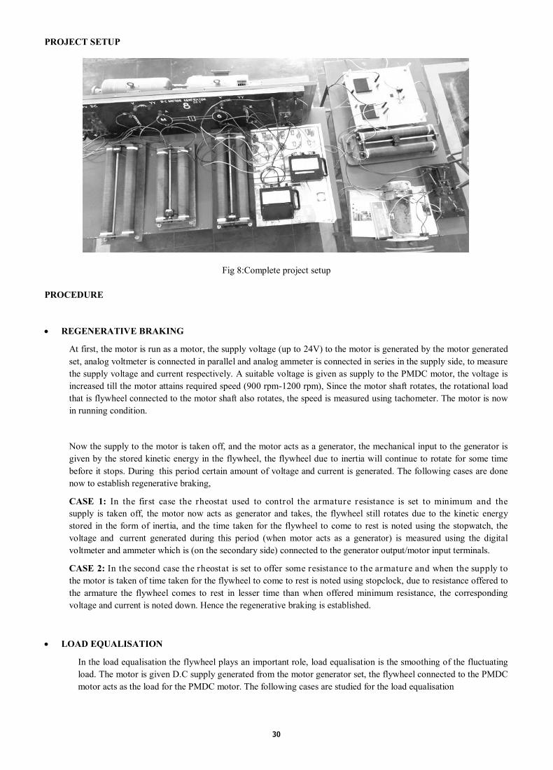
30
PROJECT SETUP
Fig 8:Complete project setup
PROCEDURE
REGENERATIVE BRAKING
At first, the motor is run as a motor, the supply voltage (up to 24V) to the motor is generated by the motor generated
set, analog voltmeter is connected in parallel and analog ammeter is connected in series in the supply side, to measure
the supply voltage and current respectively. A suitable voltage is given as supply to the PMDC motor, the voltage is
increased till the motor attains required speed (900 rpm-1200 rpm), Since the motor shaft rotates, the rotational load
that is flywheel connected to the motor shaft also rotates, the speed is measured using tachometer. The motor is now
in running condition.
Now the supply to the motor is taken off, and the motor acts as a generator, the mechanical input to the generator is
given by the stored kinetic energy in the flywheel, the flywheel due to inertia will continue to rotate for some time
before it stops. During this period certain amount of voltage and current is generated. The following cases are done
now to establish regenerative braking,
CASE 1: In the first case the rheostat used to control the armature resistance is set to minimum and the
supply is taken off, the motor now acts as generator and takes, the flywheel still rotates due to the kinetic energy
stored in the form of inertia, and the time taken for the flywheel to come to rest is noted using the stopwatch, the
voltage and current generated during this period (when motor acts as a generator) is measured using the digital
voltmeter and ammeter which is (on the secondary side) connected to the generator output/motor input terminals.
CASE 2: In the second case the rheostat is set to offer some resistance to the armature and when the supply to
the motor is taken of time taken for the flywheel to come to rest is noted using stopclock, due to resistance offered to
the armature the flywheel comes to rest in lesser time than when offered minimum resistance, the corresponding
voltage and current is noted down. Hence the regenerative braking is established.
LOAD EQUALISATION
In the load equalisation the flywheel plays an important role, load equalisation is the smoothing of the fluctuating
load. The motor is given D.C supply generated from the motor generator set, the flywheel connected to the PMDC
motor acts as the load for the PMDC motor. The following cases are studied for the load equalisation

31
CASE 1: The motor is given D.C supply, the motor starts rotating, the flywheel connected to the motor shaft
rotates, now when the motor is running the supply is taken off, the flywheel continues to rotate due to the kinetic
energy stored in the form of inertia, the flywheel is left to come to rest, when the flywheel comes to rest the supply
is again given back to the motor, now the motor draws high current and there is a large dip in the voltage, the
corresponding current and voltage is noted down from the analog ammeter and voltmeter connect to the supply
side of the motor. (due to this there is a large dip in the voltage, the motor and the equipments connected with the
same supply are affected by voltage fluctuations).
CASE 2: In this case the supply to the motor is taken off during the motor running condition, and the
flywheel continues to rotate due to the kinetic energy stored in it in the form of inertia for a period of time, now
before the flywheel comes to rest the supply is given back to the motor, the motor now draws less current and there
is less dip in the voltage as compared to the first case, the corresponding current and voltage is noted down from
the analog ammeter and voltmeter connected to the supply side of the motor, hence LOAD EQUALISATION is
established.
REGENERATIVE BRAKING
When the motor is given supply of 15V D.C, the motor draws a current of 5 amperes and rotates at a speed of 1100
RPM.
CASE 1. At minimum armature resistance offered through the rheostat(14 ohms), when the supply voltage is taken
off the flywheel continues to rotate due the kinetic energy stored in the form of inertia for a time duration of 12
seconds, the motor is now acting as a generator and produces voltage of 5V and current of 2 amperes.
CASE 2. When certain armature resistance is offered through the rheostat(14 ohms), when the supply voltage is
taken off the flywheel continues to rotate due the kinetic energy stored in the form of inertia for a time duration of
8 seconds, the motor is now acting as a generator and produces voltage of 3V and current of 1 amperes.
LOAD EQUALISATION
CASE 1. When the motor supply is taken off and the motor hence the flywheel comes to rest after some period of
time, now the supply is given back again to the motor and the current drawn and the voltage are seen and the graph
is plotted.
Fig 9:Graph for large current drawn by motor
CASE 2. When the motor is given the D.C supply the motor rotates hence the flywheel, the supply is taken off,
the flywheel rotates due to the kinetic energy stored in it, the flywheel continues to rotate for some period of time,
the supply is given back to the motor before the flywheel comes to rest, now the current drawn by the motor is
observed and the graph is plotted.
4. RESULTS

32
Fig 10:Graph of low current drawn by the motor
Advantages of Permanent magnet DC motor
Permanent these motors do not require external excitation for producing magnetic fields. Thus there is saving in
energy required for creating magnetic fields.
As the windings on the field are absent, the size of such motor is small as compared to equal rating conventional
motor.
The cost of these machines is low, Cheaper and economical for fractional KW rated applications.
The efficiency of these motors is high compared to conventional motors as the field losses are absent.
The motors designed up to 12V or less produce less TV and radio interference.
These motors produce less air noise.
Advantages of Regenerative Braking
The Energy conservation
The flywheel absorbs energy when braking via a clutch system slowing the car down and speeding up the wheel. To
accelerate, another clutch system connects the flywheel to the drive train, speeding up the car and slowing down the
flywheel. Energy is therefore conserved rather than wasted as heat and light which is what normally happens in the
contemporary shoe/disc system.[2][3][4]
Wear reduction
An electric drive train also allows for regenerative breaking which increases efficiency and reduces wear on the
vehicle brakes. In regenerative braking, when the motor is not receiving power from the battery pack, it resists the
turning of the wheels, capturing some of the energy of motion as if it were a generator and returning that energy to
the battery pack. In mechanical brakes, lessening wear and extending brake life is not possible. This reduces the use
of the brake.[4]
Fuel consumption
The fuel consumption of the conventional vehicles and regenerative braking system vehicles was evaluated over a
course of various fixed urban driving schedules. It has been proved the regenerative is very fuel efficient.
Approximately 20-25% saving in fuel consumption.[4]
Braking is not total loss
Conventional brakes apply friction to convert a vehicle’s kinetic energy into heat. In energy terms, therefore, braking
is a total loss, once heat is generated, it is very difficult to reuse. The regenerative braking system, however, slows a
vehicle down in a different way.[4]
Advantages of the Project
With the use of PMDC motor in regenerative braking, the kinetic energy of vehicle lost during braking can be
converted to electricity.
Since we are using PMDC motor, the use of rectifiers in case of alternators can be eliminated.
With load equalisation, the electrical power from the supply remains constant. Which helps in the protection of the
electrical appliances which are connected to the same source from voltage fluctuation.[5]
Eco friendly, pollution free Green energy.
5. ADVANTAGES

33
Regenerative braking system used in the vehicles satisfies the purpose of saving a part of the energy lost during braking.
Also it can be operated at high temperature range and are efficient as compared to conventional braking system. The results
from some of the test conducted show that around 30% of the energy delivered can be recovered by the system.
Regenerative braking system has a wide scope for further development and the energy savings. The use of more efficient
systems could lead to huge savings in the economy of any country. Load equalization is used in the fluctuating loads so that
there is no high voltage fluctuations in the equipment, the life of the equipment is increased and the power loss is reduced.
1. “Regenerative Braking Characteristics of PMDC Motor by Applying Different Armature Voltage”- S.M. Baque
Billah, Dr. Kazi Khairul Islam, 2nd International Conference on Electrical, Computer & Telecommunication
Engineering (ICECTE) 8-10 December 2016, Rajshahi-6204, Bangladesh.
2. “Review on Regenerative Braking Methodology in Electric Vehicle” Yogesh Abhale, Prateek Nigam, International
Journal of Advanced Research in Electrical, Electronics and Instrumentation Engineering, Vol. 4, Issue 7, July 2015.
3. Electricity Generation through Wheel Regenerative Braking System-Pratibha Patel, Upwan Kumar Sahu, Veena,
Rashmi Khutel, Juli Singh Sadhak, International Journal of Engineering Science and Computing, April 2016 Volume
6 Issue No. 4.
4. ”Regenerative braking systems(RBS) (Future of braking systems) – Pulkit Gupta, Anchal Kumar, Sandeepan Deb,
Shayan, International Journal of Mechanical And Production Engineering, ISSN: 2320-2092, Volume- 2, Issue- 5,
May-2014
5. “Fundamentals of Electrical Drives” – Gopal K. Dubey, 2nd Edition.
6. CONCLUSION
REFERENCES

34
REAL POWER LOSS REDUCTION BY PRECOCIOUS PARTICLE SWARM OPTIMIZATION ALGORITHM
K Lenin Professor
Prasad V. Potluri Siddhartha Institute of Technology
Kanuru, Vijayawada, Andhra Pradesh -520007
Email : [email protected]
This paper presents Precocious Particle Swarm Optimization (PPSO) algorithm for solving optimal reactive power problem.
Particle Swarm Optimization algorithm maintains a swarm of particles, where each particle has position vector and velocity
vector which represents the potential solutions of the particles. These vectors are modernized from the information of global
best (Gbest) and personal best (Pbest) of the swarm. All particles move in the search space to obtain optimal solution. In
this paper a new concept is introduced of calculating the velocity of the particles with the help of Euclidian Distance
conception. This new-fangled perception helps in finding whether the particle is closer to Pbest or Gbest and updates the
velocity equation consequently. By this we plan to perk up the performance in terms of the optimal solution within a
rational number of generations. Projected Precocious Particle Swarm Optimization (PPSO) algorithm has been tested on
standard IEEE 57 bus test system and simulation results show clearly about the better performance of the proposed
algorithm in reducing the real power loss with control variables are within the limits.
Keywords: Particle swarm, Precocious, Optimization, Optimal reactive power, Transmission loss.
Optimal reactive power dispatch problem is one of the difficult optimization problems in power systems. The sources of the
reactive power are the generators, synchronous condensers, capacitors, static compensators and tap changing transformers.
The problem that has to be solved in a reactive power optimization is to determine the required reactive generation at
various locations so as to optimize the objective function. Here the reactive power dispatch problem involves best utilization
of the existing generator bus voltage magnitudes, transformer tap setting and the output of reactive power sources so as to
minimize the loss and to maintain voltage stability of the system. It involves a nonlinear optimization problem. Various
mathematical techniques have been adopted to solve this optimal reactive power dispatch problem. These include the
gradient method [1, 2], Newton method [3] and linear programming [4-7].The gradient and Newton methods suffer from the
difficulty in handling inequality constraints. To apply linear programming, the input- output function is to be expressed as a
set of linear functions which may lead to loss of accuracy. Recently many global optimization techniques have been
proposed to solve the reactive power flow problem [8-10]. This paper presents Precocious Particle Swarm Optimization
(PPSO) algorithm for solving optimal reactive power problem. Particle Swarm Optimization algorithm maintains a swarm
of particles, where each particle has position vector and velocity vector which represents the potential solutions [11-14] of
the particles. In this paper a new concept is introduced of calculating the velocity of the particles with the help of Euclidian
Distance conception. This new-fangled perception helps in finding whether the particle is closer to Pbest or Gbest and
updates the velocity equation consequently. Proposed Precocious Particle Swarm Optimization (PPSO) algorithm has been
ABSTRACT
1. INTRODUCTION

35
evaluated on standard IEEE 57 bus test system. The simulation results show that the proposed approach outperforms all
the entitled reported algorithms in minimization of real power loss.
Active power loss
The objective of the reactive power dispatch is to minimize the active power loss in the transmission network, which can be
mathematically described as follows:
(1)
Where gk: is the conductance of branch between nodes i and j, Nbr: is the total number of transmission lines in power
systems.
Voltage profile improvement
For minimizing the voltage deviation in PQ buses, the objective function becomes,
(2)
Where ωv: is a weighting factor of voltage deviation.
VD is the voltage deviation given by,
(3)
Equality Constraint
The equality constraint of the ORPD problem is represented by the power balance equation, where the total power
generation must cover the total power demand and the power losses,
(4)
Inequality Constraints
The inequality constraintsimitate the limits on components in the power system as well as the limits created to ensure
system security. Upper and lower bounds on the active power of slack bus, and reactive power of generators;
(5)
(6)
Upper and lower bounds on the bus voltage magnitudes:
(7)
Upper and lower bounds on the transformers tap ratios:
2. OBJECTIVE FUNCTION

36
(8)
Upper and lower bounds on the compensators reactive powers:
(9)
Where N is the total number of buses, NT is the total number of Transformers; Ncis the total number of shunt reactive
compensators.
Inspired by the social cooperative and competitive behaviour of bird flocking and fish schooling, Kennedy and Eberhart
[11, 12] proposed a new optimization technique called particle swarm optimization (PSO). The motivation behind this
method was based on the simulation of animal social behaviours like fish schooling, bird flocking and many more. PSO has
drawn widespread attention in the last decades. Like other evolutionary algorithms particle swarm algorithm starts with the
random initialization of a population of individuals in the search space. But in PSO there is no direct recombination of
genetic material between individuals during the search. Therefore, it finds the global best solution by simply adjusting the
trajectory of each individual during the search. This algorithm works on the social behaviour of particles in the swarm.
Therefore, it finds the global best solution by simply adjusting the trajectory of each individual toward its own best location
and toward the best particle of entire swarm at each generation (time step). In simple language, the particles are flown
through a multidimensional search space, where the position of each particle is adjusted according to its own experience and
that of its neighbours, following two components are evaluated:
1) Position of the particle (Xid)
2) Velocity of the particle (Vid)
To calculate these two modules of PSO, a swarm of particles having position vector and velocity vector of the ith particle in
the d-dimension search space can be represented as Xi = (xi1, xi2, xi3, . . . , xid) and Vi = (vi1, vi2, vi3, . . . , vid) respectively. By
using fitness function, can be unimodal or multimodal in nature suppose the best position of each particle i.e., best fitness
value obtained by that particle at time t is Pbest = (pi1, pi2, pi3, . . . , pid) , and the fittest particle found till now at time t is
Gbest= (pg1, pg2, pg3, . . . ,pgd) . Then, for calculating the new velocities and the positions of the particles for next fitness
evaluation following equations is used:
(10)
(11)
Where c1 and c2 are positive acceleration constants used to scale the contribution of cognitive and social components
respectively and rand1 and rand2 are two separately generated uniformly distributed random numbers in range [0,1].
The first part of (10) represents the previous velocity, which provides the necessary momentum for particles to roam across
the search space. The second part, known as the cognitive component, represents the personal thinking of each particle. The
cognitive component encourages the particles to move toward their own best positions found so far. The third part is known
as the social component, which represents the collaborative effect of the particles, in finding the global optimal solution.
The social component always pulls the particles toward the global best particle found so far. Initially, a population of
particles is generated with random positions, and then random velocities are assigned to each particle. The fitness of each
particle is then evaluated according to a user defined objective function. At each generation, the velocity of each particle is
calculated according to (10) and the position for the next function evaluation is updated according to (11).Each time if a
particle finds a better position than the previously found best position, its location is stored in memory. Generally, a
maximum velocity (Vmax) for each modulus of the velocity vector of the particles (Vid) is defined in order to Control
excessive roaming of particles outside the user defined search space. Whenever a Vid exceeds the defined limit, its velocity
is set to Vmax.
3. PARTICLE SWARM OPTIMIZATION

37
In this paper we are using a new concept of closeness based evaluation on the swarm. As we know heuristic approaches
have not necessarily been proven to produce the global minimum with every trial or to be applicable in all cases. Rather,
they have been demonstrated to work well in general. Since, PSO is population based heuristic search and the speed of
population based search heuristic can be measured in iterations, function evaluations or real time. Since, each particle
evaluates its function value at each iteration the number of function evaluations conducted per iteration is equal to the
number of search agents. Function evaluation seems to be most popular measure. Real time is not generally used since the
time required to run simulation on one computer might not equal the time required on another computer, making real time
comparison from paper to paper is practically impossible.
The optimization problem is then to find values of the variables that minimizes or maximizes the objective function while
satisfying the constraints.
Generally in population based optimization method, it is desirable to encourage the individuals to wander through the entire
search space without clustering around the local optima, during the early stages of the optimization. On the other side,
during the latter stages, it is very important to enhance convergence toward the global optima, to find optimum solution
efficiently. Considering these concerns, in this paper we propose new concept of calculating the distance among the
particles which helps in determining the closeness towards Gbest or Pbest, named as closeness based method. This concept
is applied with HPSO (Hierarchical Particle Swarm Optimizer) -TVAC (Time-Varying Acceleration Coefficients) which
yields a new algorithm termed as closeness based HPSO with TVAC, which uses TVAC as new parameter strategy for the
PSO concept and on the basis of Euclidian distance between the particle and Pbest and particle and Gbest elements of the
swarm are accelerating towards the optimal solution [13]. This concept depicts the problem of minimization clearly. Firstly,
in TVAC like ratnaweera et al [14] has proposed in his work, we reduce the cognitive component and increase the social
component by changing the acceleration coefficient c1 and c2 with time. This is known as PSO-TVAC method.
Secondly, Kennedy et al [11] proposed a version of PSO without the velocity of previous iteration. Later they concluded
that since this version is very simple, it is ineffective in finding global optimal for complex problems. To overcome this
problem ratnaweera et al [14] proposed HPSO to provide the required momentum for particles to find global optimum
solution in the absence of previous velocity term in (10). Lastly, our new concept is introduced here to enhance the
performance furthermore which yields good results. The closeness is calculated with the help of Euclidian distance among
the particles. If the particle is more closer to Gbest then move that particle toward Gbest by reducing the cognitive factor c1
and increasing the social factor c2 by specific value in velocity update equation (10) else vice-versa. Hence, a significant
improvement of performance is observed with this new closeness based HPSO with TVAC method and also proves its
acceptance for minimization problem of optimization.
Precocious Particle Swarm Optimization (PPSO) algorithm for solving Reactive power problem
a. Generate arbitrary population of particle with random position and velocity in search space.
b. Set the parameters of the algorithm as:
C1_min = 0.50
C1_max = 2.44
C2_min = 0.50
C2_max = 2.50
W_min = 0.40
4. PRECOCIOUS PARTICLE SWARM OPTIMIZATION

38
W_max = 0.90
C1 = 2.50
C2 = 0.50
c. Find initial function values of the swarm by using fitness function.
d. Find the local best (Pbest) position of ith particle.
e. Find the global best (which is best among personal best (Pbest)) position of the swarm, i.e., Gbest.
f. For i=1 to Imax; Calculate the varying coefficient factors i.e., C1_var, C2_var and W_var to upgrade the acceleration coefficients
and inertia weight.
g. Calculate the Euclidian distance for each particle between
aa. Particle’s and Gbest’s position (DXG).
bb. Particle’s and Pbest’s position (DXP).
h. Update the value of inertia weight by W=W-W_var
i. Check if DXG< DXP
Then update C1 = C1 – C1_var
C2 = C2 + C2_var
Else C1 = C1 + C1_var
C2 = C2 – C2_var
j. Update the velocity (Vid) of each particle by the velocity vector equation:
k. Update the position Xid of each particle by position vector equation:
l. Update the velocity and position of Gbest particle.
m. Repeat step c to step l until termination criteria is met (maximum number of iteration).
n. Stop
Proposed Precocious Particle Swarm Optimization (PPSO) algorithm has been tested in standard IEEE-57 bus power
system. The reactive power compensation buses are 18, 25 and 53. Bus 2, 3, 6, 8, 9 and 12 are PV buses and bus 1 is
selected as slack-bus. The system variable limits are given in Table 1.
The preliminary conditions for the IEEE-57 bus power system are given as follows:
Pload = 12.010 p.u. Qload = 3.009 p.u.
The total initial generations and power losses are obtained as follows:
= 12.5032 p.u. = 3.3204 p.u.
Ploss = 0.25612 p.u. Qloss = -1.2008 p.u.
Table 2 shows the various system control variables i.e. generator bus voltages, shunt capacitances and transformer tap
settings obtained after PPSO based optimization which are within the acceptable limits. In Table 3, shows the comparison of
optimum results obtained from proposed PPSO with other optimization techniques. These results indicate the robustness of
proposed PPSO approach for providing better optimal solution in case of IEEE-57 bus system.
5. SIMULATION RESULTS

39
Table 1. Variable Limits
Table 2. Control variables obtained after optimization
Reactive Power Generation Limits
Bus no 1 2 3 6 8 9 12
Qgmin -1.4 -.015 -.02 -0.04 -1.3 -0.03 -0.4
Qgmax 1 0.3 0.4 0.21 1 0.04 1.50
Voltage And Tap Setting Limits
vgmin Vgmax vpqmin Vpqmax tkmin tkmax
0.9 1.0 0.91 1.05 0.9 1.0
Shunt Capacitor Limits
Bus no 18 25 53
Qcmin 0 0 0
Qcmax 10 5.2 6.1
Control Variables PPSO
V1 1.10
V2 1.030
V3 1.045
V6 1.032
V8 1.031
V9 1.011
V12 1.022
Qc18 0.0650
Qc25 0.200
Qc53 0.0451
T4-18 1.010
T21-20 1.052
T24-25 0.870
T24-26 0.812
T7-29 1.050
T34-32 0.880
T11-41 1.020
T15-45 1.040
T14-46 0.910
T10-51 1.020
T13-49 1.060
T11-43 0.910
T40-56 0.900
T39-57 0.950
T9-55 0.950

40
Table 3. Comparison results
In this paper, Precocious Particle Swarm Optimization (PPSO) algorithm has been effectively solved Optimal Reactive
Power problem. This new-fangled perception helps in finding whether the particle is closer to Pbest or Gbest and updates
the velocity equation consequently. Proposed Precocious Particle Swarm Optimization (PPSO) algorithm has been
evaluated on standard IEEE 57 bus test system. The simulation results show that the proposed approach outperforms all
the entitled reported algorithms in minimization of real power loss.
1. O.Alsac,and B. Scott, “Optimal load flow with steady state security”,IEEE Transaction. PAS -1973, pp. 745-751.
2. Lee K Y ,Paru Y M , Oritz J L –A united approach to optimal real and reactive power dispatch , IEEE Transactions
on power Apparatus and systems 1985: PAS-104 : 1147-1153
3. A.Monticelli , M .V.F Pereira ,and S. Granville , “Security constrained optimal power flow with post contingency
corrective rescheduling” , IEEE Transactions on Power Systems :PWRS-2, No. 1, pp.175-182.,1987.
4. Deeb N ,Shahidehpur S.M ,Linear reactive power optimization in a large power network using the decomposition
approach. IEEE Transactions on power system 1990: 5(2) : 428-435
5. E. Hobson ,’Network consrained reactive power control using linear programming, ‘ IEEE Transactions on power
systems PAS -99 (4) ,pp 868-877, 1980
6. K.Y Lee ,Y.M Park , and J.L Oritz, “Fuel –cost optimization for both real and reactive power dispatches” , IEE
Proc; 131C,(3), pp.85-93.
7. M.K. Mangoli, and K.Y. Lee, “Optimal real and reactive power control using linear programming” , Electr.Power
Syst.Res, Vol.26, pp.1-10,1993.
S.No. Optimization Algorithm
Finest Solution Poorest Solution Normal Solution
1 NLP [15] 0.25902 0.30854 0.27858
2 CGA [15] 0.25244 0.27507 0.26293
3 AGA [15] 0.24564 0.26671 0.25127
4 PSO-w [15] 0.24270 0.26152 0.24725
5 PSO-cf [15] 0.24280 0.26032 0.24698
6 CLPSO [15] 0.24515 0.24780 0.24673
7 SPSO-07 [15] 0.24430 0.25457 0.24752
8 L-DE [15] 0.27812 0.41909 0.33177
9 L-SACP-DE [15] 0.27915 0.36978 0.31032
10 L-SaDE [15] 0.24267 0.24391 0.24311
11 SOA [15] 0.24265 0.24280 0.24270
12 LM [16] 0.2484 0.2922 0.2641 13 MBEP1 [16] 0.2474 0.2848 0.2643
14 MBEP2 [16] 0.2482 0.283 0.2592
15 BES100 [16] 0.2438 0.263 0.2541
16 BES200 [16] 0.3417 0.2486 0.2443
17 Proposed PPSO 0.22008 0.23104 0.22106
6. CONCLUSION
REFERENCES

41
8. Berizzi.C.Bovo,M.Merlo,andM.Delfanti,(2012), “A GA approach to compare ORPF objective functions including
secondary voltage regulation,” Electric Power Systems Research, vol. 84, no. 1, pp. 187 – 194.
9. D. Devaraj, and B. Yeganarayana, “Genetic algorithm based optimal power flow for security enhancement”, IEE
proc-Generation.Transmission and. Distribution; 152, 6 November 2005.
10. C.A. Canizares , A.C.Z.de Souza and V.H. Quintana , “ Comparison of performance indices for detection of
proximity to voltage collapse ,’’ vol. 11. no.3 , pp.1441-1450, Aug 1996 .
11. R. Eberhart and J. Kennedy, A new optimizer using particle swarm theory, in proc. 6th Int. Symp. Micro Machine
Human Sci., 1995, pp.39-43.
12. Kennedy, J.; Eberhart, R. (1995). Particle Swarm Optimization. Proceedings of IEEE International Conference on
Neural Networks IV. pp. 1942–1948.
13. S. Yang and C. Li (Dec. 2010), A clustering particle swarm optimizer for locating and tracking multiple optima in
dynamic environments, IEEE Trans. Evol. Comput., vol. 14, no. 6, pp. 959–974.
14. A. Ratnaweera, S. K. Halgamuge, and H. C. Watson (Jun. 2004), Self-organizing hierarchical particle swarm
optimizer with time-varying acceleration coefficients, IEEE Trans. Evol. Comput., vol. 8, no. 3, pp. 240–255.
15. Chaohua Dai, Weirong Chen, Yunfang Zhu, and Xuexia Zhang, “Seeker optimization algorithm for optimal reactive
power dispatch,” IEEE Trans. Power Systems, Vol. 24, No. 3, August 2009, pp. 1218-1231.
16. J. R. Gomes and 0. R. Saavedra, “Optimal reactive power dispatch using evolutionary computation: Extended
algorithms,” IEE Proc.-Gener. Transm. Distrib.. Vol. 146, No. 6. Nov. 1999.

42
INDIAN AGRICULTURE DURING GLOBALIZATION ANALYSIS OF IMPORT & EXPORT OF SEEDS
AND FERTILISERS
Sandeep Bhattacharjee Assistant Professor
Amity University,Kolkata
Major Arterial Road, Action Area II, Kadampukur Village
Rajarhat, Newtown, Kolkata, West Bengal 700156
Mobile: +91-9836648495
E-mail:[email protected]
Agriculture is one of the fundamental occupation which has formed the backbone of India’s economy since ages. Moreover,
globalization has a major impact on all sectors of the Indian economy including agriculture. It forms both input for other
food firms across India, as well as one of the majorly exported commodity to other parts of the world. This sector also
requires imports of seeds and fertilsers to invigorate higher crop yields for domestic consumption and exports also. In this
research article, we have tried to understand the major imports and exports in the agricultural sector. We have also tried to
understand and investigate the merits and demerits of agriculture due to globalization.
Keywords: Agriculture, imports, exports, seeds, fertilizers.
1.1 Globalization in India Globalization has brought speedy changes at the international level. Due to the
modernized and refined means of communication and new technology many areas like production, ideas, working methods
and other traditional things are fast becoming obsolete. The process of globalization is captivating the developing countries
to participate and follow its trends. It tends to strengthen international financial organization so that they can interfere in the
affairs of these countries. The process of globalization influences economy, communication, politics and culture. All these
things have become more interconnected in the whole world and the culture of universalization is grabbing all around us. In
India the growth rate was never more than 6% in 1990 decade. Before that the average growth rate was only 3%. In the
decade of 1990, the situation was stable which was conducive to experiments with policies of liberalization, globalization,
economic reforms and new experiments. At this time our foreign exchange reserves were close to zero. Now we have
almost 120 lakh dollars as foreign exchange reserves. Some states (ELK Asia Pacific Journals – Special Issue ISBN: 978-81
-930411-9-2) benefited from these polices of 1990 but other states like Bihar, Orissa , Chhattisgarh, Jharkhand, etc have not
been able to adjust to these reforms. That is why there is no development in states nor has poverty decreased. The end result
is that globalization has helped multinational companies more than the poor population of India.
1.2 Current Status of Indian Agricultural sector Share of agriculture in the GDP of the country is only 12.6% in
2013-14. The productivity chart of India is still low as compared to some other developed nations, considering the fact that
ABSTRACT
1. INTRODUCTION

43
more than 60% of total land area is under cultivation. It remains the largest contributor towards disguised unemployment in
the country. Despite the agriculture ministry providing a high budget towards development of irrigation facilities, most
farmers still depend on rainfall for their irrigation needs. Agriculture sector is changing the socio-economic environment of
the population due to liberalization and globalization. About 75% people are living in rural areas and are still dependent on
agriculture. Agriculture continues to play a major role in Indian economy.
1. To identify exports of seeds, fertilizers.
2. To identify foreign imports of seeds, fertilizers.
3. To make comparison between domestic and imported seeds, fertilizers.
4. To suggest improvements for higher growth of agro-inputs in Indian agriculture.
Hirstet al. (2008) illustrates that globalization is nothing new, that it refers to an old process that began more than 100 years
ago. The commencement of these processes can be associated to the second half of the nineteenth century, when due to
technical and technological innovation, industrial revolution, the importance of transportation, costs were considerably
reduced. Hill (2009) explained that globalization refers to the move towards a more integrated and interdependent world
economy, due to the decline in barriers of the free flow of goods, services and capital after the end of World War II and the
wave of technological change as key factors. Cerny (2011) explained globalization as a complex set of economic and
political structures and processes created from the changing nature of the goods and assets that made up the base of the
international political economy more in focus, the increasing structural segregation of those goods and assets. Stiglitz
(2012) describes globalization as the faster integration of the countries and citizens of the world as a result of the enormous
reduction of costs of transportation and communication, and the flouting down of artificial barriers to the flows of goods,
services, capital, knowledge, and also people across borders.
The aforesaid study is based on the secondary data. The data were collected, analyzed and disseminated from various
secondary sources such as Economic Survey, Govt. of India, Books, Journals, Articles, Yojana and various websites.
5.1 Indian seed industry
Fig. 1 Area versus Arable land, Year 2014
( Source: Agriculture Statistics at a Glance, 2014;Food and Agriculture Organisation on United States)
2. OBJECTIVES
3. LITERATURE REVIEW
4. METHODOLOGY AND DATA SOURCES
5. DISCUSSION

44
Global seed industry is estimated at USD 45 billion (ISF, 2013) and Indian seed industry is ranked 5th in the world in value
terms accounting USD 2.2 Billion (5%) with major growth from Cotton, Rice and Vegetable seeds. India with 48% of its
land being arable and its population employment under agriculture being 55% clearly reflects the agriculture sector to be
the mainstay of Indian Economy (ICRA,2015).
5.2 Seed exports from India
Fig 2. Vegetarian seeds exports, Year 2013)
(Source: http://news.agropages.com/News/NewsDetail---18551.htm)
India ranks 26th globally with annual seed export of USD 138 Million including field crops around USD 71 million and
vegetable crops around USD 68 million. Vegetable crops seed are mainly exported to Asia-Pacific (about 57%), Europe
(23%) and North America (12%). About 8% of the total vegetable seed export goes to Africa (APEDA,2013).
5.3 Fertilizers in India
Fig 3. Installed capacity of fertilizers in India, Year 2013
(Source: http://www.krishijagran.com/farm-data/indian-fertilizer-sector-at-a-glance/)

45
India has around 30 manufacturing units of Urea with an Installed capacity of 21.6 million tonnes till 2013. There are 12
units of DAP (di-ammonium phosphate) producing plants with a combined capacity of 8.3 million tones ( year 2013).
Complex fertilizers in the country have installed capacity of 6.4 million tonnes from 19 units. Maximum number of
fertilizer units in the country belongs to SSP (single super phosphate). India has 85 SSP units with a combined production
capacity of 7.7 million tones.
5.4 Fertilizers production in India
Fig 4. Production status of different fertilizers, Year 2008 to 2013
(Source: http://www.krishijagran.com/farm-data/indian-fertilizer-sector-at-a-glance/)
India ranks third in the world of fertilizers production. India is meeting 80 per cent of its urea requirement through
indigenous production but is largely import dependent for its requirements of phosphatic and potassic (P & K) fertilizers
either as finished fertilizers or raw materials. Its entire potash requirement, about 90 per cent of phosphatic requirement, and
20 per cent urea requirement is met through imports. ( as seen in figure 4).
5.5 Growth trends:
Table 1. Annual Average Growth Rate in Agriculture & Overall GDP ( in Percent)
Source: Economic Survey,G.O.I.,2007-2008 and 2012-2013. (N.A = Not Available)
Rate in Agriculture & Overall
GDP ( in Percent) Five Year Plan
Overall GDP
Growth Rate
Growth Rate in GDP of
Agriculture & Allied Sectors
7th Plan 1985 – 1990 6.0 3.2
Annual Plan 1990 – 1992 3.4 1.3
8th Plan 1992 – 1997 6.7 4.7
8th Plan 1992 – 1997 5.5 2.1
10th Plan 2002 – 2007 7.6 2.3
2002 – 2003 3.8 7.2
2003 – 2004 8.5 10.0
2004 – 2005 7.5 0.00
2005 – 2006 9.0 6.00
2006 – 2007 9.2 2.7
2010 – 2011 N.A 7.9
2011 – 2012 N.A 3.6

46
As seen in the table 1, The Growth in agriculture GDP which stood at 4.7 per cent per annum during the 8th Plan (1992 –
97) progressively declined to 2.1 per cent per annum during the 7th Plan (1997 – 02) and 1.8 per cent annum during 10th
Plan (2002 – 07) and 3.6 percent annum during the 11th plan. The growth in agriculture and allied sectors has fallen short of
the Eleventh Plan target. The average annual growth in agriculture and allied sector is placed at 3.6 per cent as against a
target of 4.0 per cent in the Eleventh Plan. Given the obvious limitation in coverage of area, long-term growth primarily
depends technology diffusion across regions. An important factor affecting this is the level of gross capital formulation in
agriculture. The proportion of gross capital formation (at constant 2004-05 prices) to the value added in agriculture sector
rose to 19.8 per cent in 2011-12 from a level of 16.1 per cent in 2007-08. However, the share of agriculture and allied
sector’s gross capital formation in overall gross capital formation of the economy has exhibited a mixed trend. Government
has also strived to enhance the flow of credit to the agriculture sector. In recent years actual credit to agriculture sector
exceeded the targets set in this regard. In 2012-13, as against a target of` 575000 crore, the actual credit to agriculture was
placed at ` 239629 crore as of September 2012. on yields in crops. This has been sought to be achieved through incremental
productivity.
5.6 Future Predictions:
Fig 5. India’s GDP predictions based on historical data
(Source: https://tradingeconomics.com/india/gdp-from-agriculture/forecast)
As seen in figure 5, we can see the future estimation of India’s GDP from agriculture which is around 4000 billion INR in
the fourth quarter of 2017-2018 annual financial year.
5.7 Pro’s and cons of Globalization :
The Positive impacts of globalization on Indian agriculture are as under :-
1) Increase National Income – Receiving the international market for the agricultural goods of India, there is an
increase in farmer’s agricultural product, new technology, new seeds etc. helped to grow the agricultural product.
2) Increase in employments – While exporting agricultural products it is necessary to classify the products, its
standardization and processing, packing etc. The industries depending on agriculture are stored and it made on
increase in employments.
3) No need to reduce the grants – According to the condition of agricultural agreement limit for grants is decided 10%
of the production value for the developing countries. But the economical grants we are received less than 10% so there
is no need of reduction.
4) Increase in the share in trade – Because of the conditions of WTO all of the countries get the same opportunities
so there is an increase in the export of agricultural products.
5) Increase in the export of agricultural goods – The prices of agricultural goods are higher in the international
market than Indian markets. If the developed countries reduced grants, they have to increase in the prices. So there will
be increase in the export in Indian market and if the prices grow, there will be profit.

47
The Negative impacts of globalization on Indian agriculture can be as follows:-
1) Grants distributed on large scale by the developed countries – Before the reduction in grants by WTO,
developed countries had distributed grants on large scale. They had grown the amount of the grants on large scales in
agriculture during 1988-1994. So they have not to face many difficulties if there is a reduction in grants.
2) Small production field – In India 60% of population depend on agriculture. The pressure on agriculture is
increasing because of the increasing population. Possession of land is small and so the production cost is higher. There
is also the problem of standard etc. So there are unfavourable impact occur on Indian agriculture.
3) Intellectual property right: - Intellectual property right cause unfavourable impacts on Indian agriculture.
Multinational companies can easily enter in the field of agriculture and it will be bad for the margin farmers.
4) Increasing production expenditure and low cost of goods – farmers are being bankrupt because of growing
production expenditure, costly seeds, on the one side and reducing prices of goods on the other side. He doesn’t let out
of it and so he is committing suicide. This can be one of the impacts of agricultural agreement.
From the above discussions, we can conclude the following :
a. Agriculture still continues to be the main industry in India but India still needs to produce more to meet the demand
requirements for certain crops from different countries around the world.
b. India’s major seeds are exported to asia pacific countries ( as seen in figure 2.).
c. India has a substantial number of fertilizer producing units for urea, DAP, complex fertilsers, SSP ( AS SEEN IN
FIGURE 3) but more units must be installed with very high demand arising in both domestic and international
agriculture markets.
d. Urea requirement is being met by indigenous production although many of the advanced fertilizers are being imported
from global fertilsers companies ( Monsanto).
The current work is restricted to the peripheries of secondary data collected from various internet sources.
We can further include more data from other relevant sources which further improve the quality of the research article.
1. Agriculture Statistics at a Glance, 2014;Food and Agriculture Organization on United States.
2. http://news.agropages.com/News/NewsDetail---18551.htm
3. http://www.krishijagran.com/farm-data/indian-fertilizer-sector-at-a-glance/
4. http://news.agropages.com/News/NewsDetail---18551.htm
5. Economic Survey,G.O.I.,2007-2008 and 2012-2013.
6. https://tradingeconomics.com/india/gdp-from-agriculture/forecast
6. FINDINGS & CONCLUSIONS
7. CONSTRAINTS
REFERENCES
8. FUTURE WORK
48
CROP RESIDUE BURNING IMPACTS ON AIR QUALITY, HEALTH AND CLIMATE CHANGE
MODELLING USING GEOSPATIAL TECHNOLOGY: A REVIEW
Himanshu Kumar Centre for Climate Change and Water Research
Suresh Gyan Vihar University, Jaipur (India)
Suraj Kumar Singh* Centre for sustainable Development
Suresh Gyan Vihar University, Jaipur (India)
*Corresponding author
Sudhanshu
Centre for Climate Change and Water Research
Suresh Gyan Vihar University, Jaipur (India)
Crop residue is a common source of air smog and poor air quality, which has adverse impacts with immediate short-term
and long-term effects on human health at local, regional and global levels. Recently, crop exercises use mechanical
harvesting machines in Indian rice and wheat farming systems. In the field of these methods, leave a large amount of plant
residues. Burning the remains of the crop, there is a general view of destroying garbage after harvesting around the world.
Crop Residue burning (CRB) is an important air pollution cause, with local, regional and global effects on air quality, public
health and climate. Globally a broad range of studies has been conducted on almost all the aspects of CRB, including its
particular types, on quantification of emissions and on calculating its numerous impacts. Hence, the object of this research
is to studies published on related topic, articles, including literature relating to field measurements, laboratory studies and
the impacts of CRB. Further, this review provides visions into the role of CRB and wildfire on air quality and health
worldwide. The MODIS on-board the Terra (EOS AM-1) and Aqua (EOS PM-1) satellites is important tool for
identification of the CRB activities over the globe. The MODIS (Terra +Aqua) retrievals provide daily global aerosol
optical depth (AOD), fine mode fraction (FMF) and Angstrom exponent (AE) over land. Based on comparative study
between AOD vs FMF and AOD vs AE, several researchers have examined the aerosol types for example urban/industrial,
CRB, dust, urban mixed etc. This review emphasis on literature findings concerning CRB emissions, the impacts on air
quality, health and climate change. And its threats to atmospheric environment and climate change.
Keywords: CRB, Geospatial Technology, Crop Residue, MODIS, Air Smog, Air Quality;
ABSTRACT

49
The easiest and most economical option is to manage the crop residue. Due to the lack of awareness or lack of appropriate
technologies, it is usually practiced everywhere. Burning the crop residues not only affects the quality of the atmosphere,
but also affects the climate and ultimately human health. Crop residues and biomass (forest fires) are considered to be the
main source of carbon dioxide, carbon monoxide, methane and nitrogen oxides [1]. Combustion of biomass is a major
source of gaseous contaminants such as carbon monoxide (CO), methane (CH4), nitrogen oxides (NOx) and hydrocarbon
troposphere. It is also an important source of aerosol in the atmosphere, which potentially affects global air quality and
climate. Impact of Rice crop burning on SPM level, SO2 and ambient air study of the effect of combustion residues in and
around Patiala, Punjab (India) [2]. It was mentioned that NO2 to increase SPM level, SO2 and combustion month (October-
November), the effects of weather parameters, especially in the direction of wind, rain, and atmospheric temperature. Most
of the particulates provided by the burning of the crop, at least PM10 and easily enter into the lungs, due to cardiovascular
problems. Generally, farmers' cultivation of crop residues is burning up to clean up their farm, weed control and has pushed
the farm, nutrient uplift agriculture or pastureland, but instead of water, it is like charcoal, liquor, gas in the form, energy
can be used as production-productive, biogas. Greenhouse gas emissions from Asian agriculture fire areas and their
transportation in air, air and vital atmospheres were measured in May-June 2009 [3]. Residues of crops are produced after
harvesting. The main reason for burning crop residues is due to the difficulty of gathering crop residues. If collected, these
residues can be used in various forms in industrial / domestic fuel, food, packaging, bedding, wall construction and green
manure etc. Many gases (SO2, NO2 and CO) etc. from combustion of crop residues also from greenhouse gases [4]. During
combustion, due to the aerosol particles emitted, the global climate has short-term cooling, while many greenhouse gases
can increase temperature (or cancellation of cooling) after several decades. Therefore, reducing combustion of biomass can
cause short-term heat without long-term cooling or temperature change. India is an agricultural country and produces a large
amount of agricultural wastes. This number will increase in the future as there is a growing population, which is necessary
to increase the productivity of agricultural waste. Biomass has been left in the agricultural residues area after grain
production. Every year the crop residues are prepared in large quantities, during harvest, in the form of leaflets and in the
form of leaf / top. Processing of agricultural products through milling also produces many waste. Agriculture is the main
business of three-quarters of the working population. It is estimated that about 500-550 Mt are formed each year in the
country. For domestic use and recycling, they are used for animal husbandry, soil exploration, biomass production, home
stoves and fuel.
2.1 Biofuel Biofuel is produced by live processes. Used for industrial or domestic energy sources, in assessing the
effects of biofuels, they should be reminded that, basically, it can be renewed so that it is "refreshing", unlike burning fat.
Biomass is more dependent on heat as the main source of energy for rural people in developing countries. In the developing
world, the number of bio-fuel in the urban areas is unknown, but it may be significant that more than 50 years from 1950-
2000, [4] estimated a 70% increase in biofuel global use, that it is now savannah After the heat is the second largest biomass
type in the world, but it is difficult to predict in the future
2.2 Agricultural/waste burning Fossil fuel and waste disposal may be common in both rural and urban areas. For
example, in other Brazilian cities, gum is the prime source of the PM. The purpose of the remaining planting is most
biomass species but this release can be very high. [5] had difficulty getting these small, small Firefox. According to the
annual crop season, remaining investment can be consumed three times in a year. Most of the biomass is used for domestic
purpose. Wood, damages and sawdust - 44 percent of biomass energy, but any living organism produces biomass energy. In
some biomass sources, agricultural products like plants and corn fruits can be included. Wood and wood are used to
generate electricity; Electrical energy sources that do waste; is not distributed by the services. Paper mills and saw mills
have used electricity and their uses to make more use of their electricity production. However, when they use more energy,
they need to buy extra power from services. Apart from the Indian part of the Gangetic plains of India mainly in Punjab and
Haryana states, agricultural residues are burnt in the northern states of India for cooking [6-8]. Moderate resolution imaging
Spectroradiometer (MODIS) and Suomi National Polar-orbiting Partnership – Visible Infrared Imaging Radiometer Suite
(Suomi NPP-VIRS) is using for Kharif Crop Season (September– November) 2014 in Punjab and Haryana states of India.
Comparative analysis of active fire detection of MODIS and VIRSS suggested that VIIRS is more sensitive with high
1. INTRODUCTION
2. TYPES OF BIOMASS BURNING

50
identification potential. Because of 15,222 (MODIS) and 15,568 (VIIRS) locations from active fire of MODIS and VIIRS in
the study area during September-November 2014. Nutrients estimate that there will be 3.85 million tonnes of organic
carbon, 59,000 tonnes of nitrogen, 20,000 tonnes of phosphorus and 34,000 tonnes of potassium. It is also an adverse result
of estimated nutrients in the soil, smoking emissions, which have added gas on the air like nitrogen oxide and ammonia,
which can be due to severe air pollution. Indirectly crop residues is also contributing to ozone pollution. These smoky
emissions may be lead to health threats, lungs, chronic bronitis and asthma [9-12].
The impact of air pollution due to the burning of agricultural residues on home cognitive health can be analysed by linking
health information to remote health information along with remote sensing data. It is observed that a significant negative
impact of fire on health is the effect: 5.1% is less in the normal cognition test in the county, with high frequencies of 55%
and above (Ages 55 and above), and 11.8% Less things are remembered [13]. This effect has been found among the
respondents living in the countries below, but not Upwing County. Cognitive impact of agricultural fire means additional
health costs that increase climate risk from climate change. To conduct the analysis, we add many datasets including remote
sensing, air quality, agricultural production, meteorological data and fire data from health data, so that we know the fire
point address: Remote sensing fire point comes from MODIS active fire product in Fire Information for Resource
Management System in NASA [14]. NASA's terra and aqua satellites has provided more than a decade of global fire data by
two Moderate Resolution Imaging Spectroradiometer (MODIS). Here describe the improvements made to recognition
algorithms and taste-level products, which were implemented as part of the collection of land product reprocessing, which
started in May 2015. The updated algorithm intends to address the borders celebrated with the previous archive 5 fire
product, especially due to the fact that false alarms are cleared of small woods, and the lack of large fire hidden from thick
smoke it occurs [15-17]. Processing of ocean and other large water bodies has also been expanded to facilitate the
monitoring of offshore gas pollution. Fire radiation power is using a glow-based approach, usually FRP decreases for all but
relatively small degrees of high intensity fire pixels. We did a Stage-3 verification of Collection 5 and Collection 6 Terra
MODIS Fire Products with a collection of reference of Fire Maps obtained from images of more than 2500 high-resolution
Advanced Space Benefit Thermal Emissions and Reflection radiometer (Aster).
The fast-changing dynamics of satellite-based terrestrial satellites and the Himawari-8 Advanced Himawari Imager (AHI)
provide unmatched views of Asian and Australian lighting at 10 m pitches and heat sinks. Minimum 2 km spatial resolution.
Developed a first-of-its-kind processing system to identify the active fire and repossess their fire radiative power (FRP)
based on AHI data using Fire Thermal Anomaly (FTA) algorithm. (Geostationary Fire Anomaly (FTA)) and FRP retrieval
method developed for use with Meteosat SEVIRI [18]. VIIRS will show you how to detect and use the new Active
Detection (AF) feature for use with the Space Sensor. In order to provide both AF notice and FRP (Fire Radiation Strength)
both to the 375-meter I-Band and the first of 750 m M-band data to provide complete fire and FRP magnitude on fire (fire
radiation power). High-sensitivity I-band VIIRS data 'Sensitive to fire' has the ability to detect small active fire (FRP ≤
1MW), but this sensitivity can cause false alarms, which is often associated with man-made structures. To protect them by
using 30 meters of worldwide coverage and an open road map mask [19-20].
It is important to assess the causes and effects of forest fires in the forest ecosystem. A simple algorithm for burning and
Burned Area Extraction and Dating (BAED) has been developed to automatically date firefighting for the wound and for
each burning cycle. The buried girth was pulled out of a two-phase method, which included determining the primary
burning pixel size and the size of the patches that were continuously burned ingredient Meteorological and Temperament is
controlled by the General Index Index. The expected fire date for each fire is given when the difference between the
observed NDVI and the predicted NDVI is predicted to increase three consecutive times [21]. With the chemical
composition of the particles of smoke emitted by the development of physical and water properties from wheat grains, the
effects of relative humidity (RH) on these properties in the aerosol room have been investigated. Particles of smoke are
made up of carbon dioxide and exotic salts (~ 25%). In the age, the inorganic salts of the inorganic salts are increased by
PM1.0 due to the formation of sulfate and nitrate. Up by the chloride value. The reduction in the density of PM2.5 and PM
1.0 will gradually increase from 1.18 to 1.44 grams per cubic meter and within 4 hours 45% E 55% RH. However,
according to the results obtained from both particle size analyzers of aerosol particle mass analysis (APM) and high density
densities by structure can solve the problem of particle density analysis from the estimation [22]. Density of smoke particles
3. MONITORING OF BIOMASS BURNING

51
depends on relative humidity and aging. Size results will not be noticeable by age. General settings and processes The effect
of relative humidity on the aging of the smoke particles in the dark results in exhaust emissions in the aerosol room from
burning wheat straw.
In many cities in India, air pollution is higher than national and international standards, and effective pollution control
strategies require knowledge of the sources that cause air pollution and suffering variability. In this study, we investigated
the impact of external combustion sources on Knik biomass matter (PM), surface visibility and optical depth (AOD) in 2013
from India's third 2007 year. In most populated cities Are you there we define a space in the atmosphere or "air hues" for
the city using the orbital trajectory behind the HVSPLIT model. As a measure of fire by using the Rediyetiv Power Satellite
(FRP) satellite, observe us monsoon after. The target before the monsoon and the monsoon fire up the national metropolitan
areas of New Delhi and Bangalore and around Pune on the east side are the fire. We found that less important work in
fiberglass air quality for individual works revealed the opposite, before the metric monsoon season, burning with outdoor
light, three different air quality. In addition, we provide a 99% share of FRP since the post-spring monsoon flare to burn
agriculture in the average fresh air of Delhi [23]. Protection does not include a good amount of practice, often soil
preparation, crop residues on the soil surface after harvesting and growing, usually improve soil organic soil (SOC)
composition and reduce soil erosion. Remote-sensing methods have shown great promise in evaluating plant residues and
have resulted in an estimated concentration of tillage. It is expected that the severity of tillage in C soil is greater than 4,200
soil and reflects 80 plant scavengers measuring the spectrum at 350 to 2500 nm wavelength region in the laboratory. Lignin
Cellulose Absorption Index (LCA) Normal Difference Index Tilj (Anditiai) Normal Difference Senesent Plant Index
(Andisviai) The six known remote senses have been used index spectrum Soil and SoC are affected for debris, so the
spectral index, which is higher than the soil classification, is often less effective. Reflection on the spectrum The spectral
index of the soil is similar to that of land resources, and in particular, the critical resource area. CAI shows the best soil and
crop waste, followed by LCA and NDTI [24].
Crop Residue can affect soil quality, global carbon balance and crop yield. This study was designed to evaluate samples of
local and temporal diversity in three areas of northern China and three areas in the northeast. Based on the crop yield data
on provinces and provinces, cereals, maize and wine - the most important source of trade is the mid-105.7 meter house with
92.8 meters and 12.9 million tons. In the average, 2008, 2009 and 2010, the SCCE was 46.4 million 42.4 meters and setting
the NEC 95 MT, which was 49.7 lakh tonnes and 7.4 MT of cheerful and September production. From October to
December, local views have been displayed in July. In September, the rest of the remaining 40.9 and 53.1 metric tons in the
NC and NEC areas [25]. Biomass burns as a major contributor in wind conditions because it has the effect of ozone and
clinical problems. Burning, part of the individual section of the initial crop, the National Inventory Institute summarizes the
summary of new perspectives to assess the outstanding homes for sensitive information and regional information. We will
pay attention to later harvesting and deforestation to distribute thin colors, maize, cotton, rice, soyabean, donkeys and
wheat. Estimates show that 5.8 million residential fire-weather acre and 53,000 smaller tonnes above the PM2.5 compared
to the United States (Conceus). Production estimates for 2007 show that during the season, 6 million acres and PM 2.5 were
being burnt in the rest of the country. To produce the material 58,000 small tones the first summit is being used with the
results of the chemical transport model. The use of CMUE version 5 (beta release) is a complete construction of the
chemical transport model for the October, October and 2006 predictions in September 2006, which is used in November
2006 for the use of survival water. Accept the specifications provided for the device, compared to a chemical transmission
model for a few years, this can easily be a good way to reduce the snow at a lower cost. Finally the results were examined
using the CMAQ5 beta version [26].
More or less all the cities of the world, air pollution in large cities leads to dirty air due to the use of rapidly growing
vehicles. Citizenship is changing the lifestyle of people, as well as serious problems related to health and environmental
harm. Hysplit4 simulation software, which is used to prevent pollution and concentration. The pollution is found in relation
to weather data (air speed, direction, temperature), because pollution runs according to local air patterns and speeds Is.
Meanwhile, the concept of continuity is artificial to assess the quantity of pollution in specific geological area. According to
the presence of pollution, both plots are for special study areas. The production of these plants will help environmental
experts to plan the industrial site, safe fireplace height for road planning. The paper has been estimated that the speed of
4. POLLUTANTS FROM BIOMASS BURNING

52
pollution and the wind direction and the wind velocity. Plot for advanced PMLO in Coablotter has been planted. All
pollution is normal. With these plants, cities planning and other buildings can be done effectively to establish industries. It
will also help in the disaster management caused by air pollution [27]. The crop residues reduce the agrochemicals in the
soil and protect the soil and runoff water. The characteristics of the absorption associated with cellulose and lignin are
different from crop residues and soil. Assess the effects of soil and crop residues on remotely estimated estimates of crop
residues and propose a method for reducing these effects. Various crops and soil reflective spectra have been acquired in the
laboratory and analysts have expanded in the agricultural sector with a wide range of cover and moisture content of various
crop residues. The slope of linear relations with cellulose absorption indicator was very sensitive to the position of moisture,
while the residual index of the short wave infrared general structure has been reduced to a lesser extent. Indicators of water,
which used to provide reliable estimation of water content, can be used to estimate the residual cover of the crop as per
moisture conditions. Water in residues and soil in the soil not only changed the reflective signal but also changed the slopes
of relations between the fraction of the residual cover and the spectral index. For the reliable estimation of the crop residual
cover, the visual water content is necessary for change. According to the previous studies, according to the estimated
estimates of the residual cover in the data set collected under the conditions of the area, using a multivariate linear model
developed from laboratory experiment. Improvement on the basis of RWC enhanced the estimation of the cover of the
residues from the CAI values and to the lesser extent from the CNRR. Changes in visible moisture limits the utility of NDTI
to cover the crop residues. Water indices provide reliable estimates of crop residues and soil water content, can be used to
estimate the residual cover of the right crop from moisture conditions. Thus, there is a need to check water indices using the
available band for many existing satellite sensors, including Landset-8, Sentin-2 and Worldview 3 [28].
Two major application will be present in using near-infrared Hyperspectral imaging (NIR-HSI), which is to coincide with
the Chemo-metrics to organize the components of the soil and to evaluate their limitations of eligibility. For the first time
during the application, the ability to use NIR-HSI to filter the residues of plants such as roots and vegetables are shown in
the soil. It is a method of estimating the levels of collagen storage during the second application of such functional strength
and used bones. The current challenges of agricultural research focus on agricultural research and the consequences of root
losses and soil residues, which are important in monitoring the development of root system and decrease in crop residues. In
this context, a study was done to use NIR-HIS and Chemo-metric tools to separate soil remains and find and measure straws
and roots [29].The temperature of biomass leads to loss of many gases and aerosols, which can damage air, weather and
human health. On the basis of domestic and tropical grasslands, wood burning, animal burning, animal burning and waste,
provincial-level work data, satellite data, and spring-release features in 2012, the heat associated with China's construction.
The review of available literature indications that the burning of waste from open crops causes emissions of air pollutants
such as particles and gases and, ultimately, influences atmospheric quality and climate. Almost all researchers agreed that
open burning of crop residues biomass significantly increases the level of particulate matter, gaseous pollutants in
atmosphere. Various research has been done using MODIS data for the monitoring of crop residue. The average size of an
agricultural burn (plot) is usually much smaller compared to MODIS of 1 km2 or 750 sq.m VIIRS footprint and there may
be more than one active combustion ground fire in the footprint of the respective sensors. The pixel aggregation scheme for
different scanning angles from the VIIRS nadir and the corresponding spatial sampling are different from those of MODIS,
which can also add to the difference in the number of fire pixels detected by each sensor for the same area of interest.
1. Sharma A.R, Kharol S.K., Badarinath K.V.S. and Singh D., Impact of agriculture crop residue burning on
atmospheric aerosol loading – a study over Punjab State, India Ann. Geophys, 28, 2010, p.367–379.
2. Singh N., Mittal S.K., Agarwal R., Awasthi A. and Gupta P.K., Impact of rice crop residue burning on levels of
SPM, SO2 and NO2 in the ambient air of Patiala (India), Intern. J. Environ. Anal. Chem., 90 (10), 2010, p.829–
843.
5. CONCLUSION
REFERENCES

53
3. Tripathi Satyendra,” International Science Congress Association Impact of Crop Residue Burning on Climate
Change: A Scenario of Madhya Pradesh, India.” Res. J. Recent. Sci. Vol. 4, 2015, p. 94-96.
4. Am J Respir Crit Care Med. “Health effects of outdoor air pollution “American Thoracic Society, Jan; 153 (1),
1996, p.3-50.
5. Moris R., Airborne particulates and hospital admissions for cardiovascular disease: a qualitative review of
evidence, Environ Health Prospect, 109, 2001, p.495–500.
6. Tripathi Satyendra, Singh R N and Sharma Shaishav.,”review Paper Emissions from Crop/Biomass Residue
Burning Risk to Atmospheric Quality” Int. Res. Earth Sci. International Science Congress Association. Vol. 1(1),
2013, p. 24-30.
7. Jacobson M.Z., “The short-term cooling but long-term global warming due to biomass burning, Journal of
Climate”, 17, 2004, p.2909-2926.
8. Niveta Jain, Arti Bhatia, Himanshu Pathak, “Emission of air pollutants from crop residue burning in India. Aerosol
and Air Quality Research, 14:, 2014, p. 422–430.
9. A. Agarwal, E. Dintwa, P. Joshi , Analysis Of Agro Residue Burning And Present Scenario In Key Areas Of
Northern Plains In India , International Journal Of Advanced Research, Volume 4, Issue 3, 2016, p. 1499-1509.
10. Thumaty, Kiran Chand; Rodda, Suraj Reddy; Singhal, Jayant; Gopalakrishnan, Rajashekar; Jha, Chandra Shekhar;
Parsi, Gururao Diwakar; Dadhwal, Vinay Kumar, “Spatio-Temporal Characterization of Agriculture Residue
Burning in Punjab and Haryana, India, Using MODIS and Suomi NPP VIIRS Data.” Current Science 109 (10),
2015, p.1850–54.
11. Parmod Kumar, Surender Kumar, Laxmi Joshi, “Socioeconomic and Environmental Implications of Agricultural,
Residue Burning,” Springer Briefs in Environmental Science, DOI 10.1007/978-81-322-2014-5_2.
12. Wangyang Lai, Yanan Li, Xiaohui Tian, Shanjun Li, “Agricultural Fires and Cognitive Function : Evidence from
Crop Production Cycles Agricultural Fires and Cognitive Function : Evidence from Crop Production
Cycles,”2017,p. 1–45. http://dx.doi.org/10.2139/ssrn.3039935
13. Louis Giglio , Wilfrid Schroeder, Christopher O. Justice, “The Collection 6 MODIS Active Fire Detection
Algorithm and Fire Products.” Remote Sensing of Environment 178. British Geological Survey, 2016, p.31–41.
14. Weidong Xu , Martin J. Wooster, Takayuki Kaneko , Jiangping He , Tianran Zhang , Daniel Fisher, “Major
Advances in Geostationary Fire Radiative Power (FRP) Retrieval over Asia and Australia Stemming from Use of
Himarawi-8 AHI.” Remote Sensing of Environment 193, 2017, p.138–49.
15. Zhang, Tianran; Wooster, Martin J.; Xu, Weidong., “Approaches for Synergistically Exploiting VIIRS I- and M-
Band Data in Regional Active Fire Detection and FRP Assessment: A Demonstration with Respect to Agricultural
Residue Burning in Eastern China.” Remote Sensing of Environment., 2017,p.407–24.
16. Zhihua Liu,Jian Yang and Francis Dwomoh, “Mapping Recent Burned Patches in Siberian Larch Forest Using
Landsat and MODIS Data.” European Journal of Remote Sensing. 49, 2016, p.861–87.
17. Chunlin Li, Zhen Ma, Jianmin Chen, Xinming,Wang, Xingnan Ye, LinWang, XinYang, “Evolution of Biomass
Burning Smoke Particles in the Dark.” Atmospheric Environment .120, Elsevier Ltd: 2015, p. 244–52.
18. Tianjia Liu, Miriam E, Marlier, Ruth S, DeFries , Daniel M., Westervelt Karen R. Xia Arlene, M.Fiore, Loretta
J., Mickley Daniel H., Cusworth, George Milly,“Seasonal Impact of Regional Outdoor Biomass Burning on Air
Pollution in Three Indian Cities: Delhi, Bengaluru, and Pune.” Atmospheric Environment (172), 2017, Elsevier: p.
83–92.

54
19. Guy Serbin , Craig S. T. Daughtry , David J. Brown , Gregory W. McCarty , “Effect of Soil Spectral Properties on
Remote Sensing of Crop Residue Cover.” Soil Science Society of America Journal 73 (5), 2009,p.15-45.
20. Lu Yang, Xiao Yu Wang, Li Pu Han, Huub Spiertz, Shu Hua Liao, Mao Gui Wei, Guang Hui Xie, “A
Quantitative Assessment of Crop Residue Feedstocks for Biofuel in North and Northeast China.” GCB Bioenergy
7 (1), 2015, p.100–111.
21. George Pouliot , Jessica McCarty, Amber Soja and Alfreida Torian, “Development of a Crop Residue Burning
Emission Inventory for Air Quality Modeling,”2012, p.1:1–7.
22. Geetha, P, and M Kokila., “Estimation of Air Pollution Using Remote Sensing Technique in Coimbatore-a Case
Study.” International Conference on Communications and Signal Processing (ICCSP), 2015, p. 0794–98.
23. Daughtry, Craig, and Miguel Quemada. 2015. “Assessing Crop Residue Cover When Scene Moisture Conditions
Change.” International Geoscience and Remote Sensing Symposium (IGARSS) 2015, p.4652–55.
24. Vincke, Damien, Eylenbosch, Damien, Fernández Pierna, Juan Antonio, Baeten, Vincent, Bodson, Bernard,
Dardenne, Pierre, “Sorting of Crop Residues and Fossil Bones From Soil By Nir Hyperspectral Imaging.”
Workshop on Hyperspectral Image and Signal Processing: Evovution in Remote Sensing,2014, p. 1–4.
25. Ying Zho, Xiaofan Xing, Jianlei Lang, Dongsheng Chen, Shuiyuan Cheng, Lin Wei, Xiao Wei, and Chao Liu, “A
Comprehensive Biomass Burning Emission Inventory with High Spatial and Temporal Resolution in China.”
Atmospheric Chemistry and Physics 17 (4),2017, p.2839–64.
26. Jianmin Chena, h , Chunlin Lia, Zoran Ristovskib, Andelija Milicb, Yuantong Gub, Mohammad S. Islamb,
Shuxiao Wangc, Jiming Haoc, “A Review of Biomass Burning: Emissions and Impacts on Air Quality, Health and
Climate in China.” Science of the Total Environment. 579, 2016, Elsevier, p.1000–1034.
27. Michael S. Christian, Adela S. Garza, Jerel E. Slaughte., work engagement: a quantitative review and test of its
relations with task and contextual performance. Vol- 68, Issue 3, 2010, p. 717–719.
28. Andreae, M.O. and Merlet, P. “Emission of Trace Gases and Aerosols from Biomass Burning. Global
Biogeochemical Cycles, 15, 2001, p.955-966.
29. Lara M, Gamboa C, Kahramanian MI, Morales LS, Bautista DE., “Acculturation and Latino health in the United
States: a review of the literature and its socio-political context.” Annu Rev Public Health. 26, 2005, p.367-97.

55
ANALYSIS AND DESIGN OF REINFORCED EARTH BED FOR A GODOWN STRUCTURE
Jayanth. K
Assistant Professor
Department of Civil Engineering
Vidya Vikas Institute of Engineering and Technology, Mysuru-570028
Shesha Prakash M N* Professor & Vice Principal
Department of Civil Engineering
Vidya Vikas Institute of Engineering and Technology, Mysuru-570028
*Corresponding author
N. R. Krishnaswamy Professor Emeritus
Indian Institute of
Technology, Chennai
In this project, Analysis and design of reinforced earth bed for a strip footing for a godown structure for storing food grains
has been conducted. Further, we have modeled the situation to arrive at a reinforcement ratio provided by the Geotextile so
that the analysis and design of a foundation on a prototype reinforcement earth bed situation can be simulated in the
laboratory with California Bearing Ratio (CBR) testing facilities. Further, it is a common practice in the design of
geosynthetic reinforced road subgrades to make use of CBR modeling. The U.S. Army corp of engineers have successfully
made use of the CBR design method to be used in the situations where geosynthetic reinforcements can be applied for the
construction of roads on very soft subgrade soils. The CBR testing is being used all over the world for the design of all
types of flexible pavements both reinforced and unreinforced since more than 50 years. The utility of CBR testing has never
diminished inspite of the scaling problems creeping into the modeling of road subgrades. This versatility of CBR testing is
made use of in arriving at an analogous situation in the analysis and design of foundations constructed on reinforced earth
beds. Here, unconfined compressive strength test conducted on the weak cohesive soil and the strength in cohesion obtained
is related to the CBR.
Keywords: Geosynthetic , Geotextile, CBR, Unconfined compressive strength
Bearing capacity is an extremely important subject of study in Geotechnical engineering. Loose sand deposits and low
quality cohesive soils have very low bearing capacities. Different in-situ improvement techniques are being used in various
Civil engineering projects with the purpose of improving the in-situ soil properties to ensure desired performance. The
performance of such soil deposits can be improved substantially by introducing reinforcing elements in it and it reduces the
construction cost by making use of locally available soil.
ABSTRACT
1. INTRODUCTION

56
Reinforced earth bed is an effective alternative to the conventional ground improvement techniques to improve bearing
capacity of weak soils. This is a soil foundation containing horizontal layers of tensile reinforcement. Such an inclusion in
the foundation soil increases the bearing capacity and the load settlement stiffness of the foundation soil system. In general
the construction of reinforced earth bed involves refilling the excavation with good quality frictional soil such as sands,
gravels or crushed stone.
Expansive soils are considered to be unsafe with reference to safety of the structure and serviceability aspects, and needs to
be tackled in a well-engineered manner, if it should be used as a foundation soil. Soil is a particulate material consisting of
soil grains and as a result it cannot withstand tensile stresses. Therefore, soils are unstable below the foundation and
undergo deformations under loads. A variety of reinforcing materials are used for reinforced earth applications. They
include natural materials, metallic strips and geosynthetics.
A reinforced soil mass is a soil mass containing reinforcement layers placed at appropriate locations in proper directions.
The bearing capacity of black cotton soil is increased with the help of geotextile soil reinforcement. The geotextile used for
this test is cement bags. Geotextile is chosen for its load carrying capacity, anti-corrodible nature, easy availability, and
economy. For road base, it is widely applied everywhere. Geotextile increases stiffness and load carrying capacity of soil
which automatically reduces the settlement of foundation.
When subjected to vertical loads, a reinforced soil mass typically exhibits higher load carrying capacity than a soil mass
without reinforcement. The present work involves analysis and design of strip footing with reinforced earth bed for a
godown structure for which raft foundation if used becomes uneconomical. This method can be implied to: Road
construction, railway construction, earth works, pipe & canal construction, examination of foundation fillings. The main
aim is to reduce load bearing problem by reinforcing expansive soil using geotextile.
To achieve the economy and for proper performance of foundation, it is necessary to improve the soil. This study
demonstrates the study of ground improvement techniques. Developmental activities in cities have lead to increased
building construction.
The main objective of this work is to study the behavior of footing on expansive soil bed with and without reinforcement,
and to find out improvement in bearing capacities. Ultimate bearing capacity can be found to increase, even with single
layer reinforcement for the footing. The effectiveness of geosynthetic reinforcement in improving the bearing capacity is
attributed to location and width of the reinforcement in the case of single layer reinforcement whereas in multilayer
reinforcement, spacing of reinforcement play significant role apart from loading applied for reinforcement. Provision of first
layer of reinforcement at a depth beyond the width of footing is not effective in improving the bearing capacity.
In the present study we have used sand as subsoil overlain by the geotextile reinforcement and a clayey base course layer.
The subgrade/base course soil is assumed to be saturated and to have a low permeability.
The unconfined compressive strength test is conducted and the cohesion value obtained is related to the CBR value. From
the unconfined compressive strength obtained, the cohesive strength of the soil is arrived and finally the CBR of the soil is
obtained (Reference: Design with Geosynthetics, Robert M. Koerner, and Fig. 2.35).
Further, referring to the work on Bearing capacity analysis of reinforced earth beds by Jean Binquet and Kenneth L.Lee,
analysis and design of reinforced earth bed for a strip footing for a godown for storing food grains has been made.
2. PROBLEM CONSIDERED

57
2.1 Tests conducted in the laboratory Various index and engineering properties of the silty clay have been
determined as per the guidelines of the Indian standard code such as,
1. Specific gravity
2. Atterberg’s limits
3. Standard proctor compaction test
4. Unconfined compressive strength test
Table 1: Soil Properties investigated.
The soil properties obtained above, suggests that the soil stratum is very weak and hence using geotextile layers as
reinforcement improves the bearing capacity. Further, we are proposing strip footing with geotextile reinforcement instead
of raft foundation.
A reinforced earth bed contains horizontally placed layers of reinforcement, in the form of thin metallic strips or
Geosynthetic mats (Geotextiles in the present case). The reinforced earth bed is an effective ground improvement technique
which enables embankments and footings to be built on very weak soils.
In reinforced earth bed, the horizontally placed reinforcements frictionally interact with the soil mobilizing interfacial shear
stresses opposing the lateral flow of soil. The mobilized interfacial shear stress will induce tension in the reinforcement. In
turn, this tension in the reinforcement opposes the downward movement of the embankment or the footing itself. The
tension in the reinforcement is variable with distance, being zero at the farthest end. The locus of the points of maximum
tension in the reinforcements can be treated as the plane separating the vertical downward and lateral movements.
BINQUET and LEE (1975) have assumed the boundary between the downward and the outward moving soil zones to be
along the plane of maximum shear stress. At shallow depths, the plane of maximum shear stress almost coincides with the
vertical plane through the edge of the footing.
Fig 1: Godown Foundation Fig 2: Footing details
Liquid limit (%) 58.50
Plastic limit (%) 40.16
Maximum dry density (kN/m3) 16.50
Optimum moisture content (%) 25.30
Specific gravity 2.64
Soil classification from plasticity chart CH-MH
Cohesion, Cu (kN/m2) 46.42
CBR of Unreinforced soil (%) 1.547
CBR of Reinforced soil (%) 1.779
BCR 1.149
3. DESIGN OF REINFORCED EARTH BED

58
Design of a strip footing on a weak silty-clay (CH-MH) to carry a line load of 2000, 2500 and 3000 kN/m for an allowable
settlement of 25 mm has been considered.
Unit cohesion, Cu= 46.42 kN/m2
Soil modulus, Es = 34000 kN/m2 for a line load of 2000 kN/m
= 36000 kN/m2 for a line load of 2500 kN/m
= 38000 kN/m2 for a line load of 3000 kN/m
Soil poisson’s ratio, μ = 0.30
Case 1:
Live load = 2000 kN/m
Unit weight of backfilled soil, γ (kN/m3) = 16 kN/m3
Angle of shearing resistance (ϕ) =350
Interfacial friction angle (δ) = 290
Number of layers (N) = 5
Assuming LDR = 1.0 (reinforcement used is geotextile)
Now for =350, Nc=46.4, Nq=33.6, Nγ=37.8
With a Factor of Safety, F.S = 2.0
Settlement criteria:
BCR = 4.76
Tension developed (Td):
The graph below gives the value of the dimensionless forces I, J and M depending upon the depth ratio
The graph below gives the value of the dimensionless lengths Lo/B and Xo/B depending upon the depth ratio.
2
13
0.67 m, 0.4 m, v=0.3m
u B B
u u
2
o,ult
20002000kN/m
1.0
0.5 q
q
q BN DN
1
, v1o
Z Z qT d N J B I
N B B q
ZB
ZB

59
Fig 3: Dimensionless forces for reinforced soil bed bearing capacity calculations
Fig 4: Dimensionless lengths for reinforced soil bed force component calculations
0.4
0.3
0.2
0.1
0.0
0 1 2 3 4 5
Depth ratio,Z
b
JZ
D
MZ
B
IX
B
Dim
ensi
on
less
Fo
rces
(M
.Z)
5
4
3
2
1
0
0 1 2 3 4 5
Depth ratio,Z
B
oL
B
oX
B
Le
ngt
h r
atio
s (L
o/B
, Xo/
B)

60
Frictional resistance mobilized:
Clearly we can see from the table
so design is safe against pullout
F.S1=Installation damage (1.1-2.0)
F.S2 = Creep (2.0 – 4.0)
F.S3 = Chemical elongation (1.0-1.5)
F.S4 = Biological degradation (1.0-1.3)
Accordingly a geotextile has to be choosen.
f
f All
2 tan L.D.R.
And F.S.
o o
o
o
f
L XZ qT M B q
B q Z D
TT
allTable 3: Calculation of an ca :d se 1f fT T
Layer No: 1 2 3 4 5
Z (m) 0.4 0.7 1.0 1.3 1.6
Z
B 0.4 0.7 1.0 1.3 1.6
Z
BI 0.25 0.22 0.18 0.14 0.12
Z
BJ 0.35 0.35 0.34 0.34 0.34
Td (Z, N) kN/m 86.8
6
89.7
0
90.3
3
94.1
2 96.01
from graph oX
B 0.5 0.6 0.7 0.95 1.10
Xo for B = 1m 0.5 0.6 0.7 0.95 1.10
from graph oL
B 1.5 2.0 2.6 3.0 3.3
Lo for B = 1m 1.5 2.0 2.6 3.0 3.3
Z
BM 0.13 0.14 0.14 0.15 0.16
Tf (kN/m) 312.95 352.50 377.69 393.92 411.74
Tf,all (kN/m) 156.48 176.25 188.85 196.96 205.87
f all ;dT T
maxult 1.5 3.0 1.25 1.2 648.07 kN/mdT T

61
Case 2:
Live load = 2500 kN/m
Unit weight of backfilled soil, γ (kN/m3) = 17 kN/m3
Angle of shearing resistance (ϕ) =380
Interfacial friction angle (δ) = 320
For = 380, Nc = 61.4, Nq= 48.9, Nγ = 64.0
Settlement criteria:
S = 34.76mm > 25mm
For satisfying this criteria the value of qo,all should be accordingly chosen
BCR=5.06
Frictional resistance mobilized:
Comparing T f,all and Td, Tf,all> Td
So design is safe against pullout failure.
Tult = 823.97 kN/m
all
all
2o
o
1 1 0.09 20.025 or
360494.5
000 kN/m
Table 4: Calculation case 2f :oZ
MB
Layer No: 1 2 3 4 5
Z (m) 0.4 0.7 1.0 1.3 1.6
Z
B
0.4 0.7 1.0 1.3 1.6
Z
BI
0.25 0.22 0.18 0.14 0.12
Z
BJ
0.35 0.35 0.34 0.34 0.34
Td (Z, N) kN/m 110.42 114.03 114.84 119.68 122.07
from graph 0.5 0.6 0.7 0.95 1.1
Xo for B = 1m 0.5 0.6 0.7 0.95 1.1
from graph 1.5 2.0 2.6 3.0 3.3
Lo for B = 1m 1.5 2.0 2.6 3.0 3.3
Z
BM
0.13 0.14 0.14 0.15 0.16
oX
B
oL
B
Tf (kN/m) 436.26 488.35 518.52 569.23 621.85
Tf,all (kN/m) 218.13 244.18 259.26 284.62 310.93
allTable 5: Calculation of an ca :d se 2f fT T
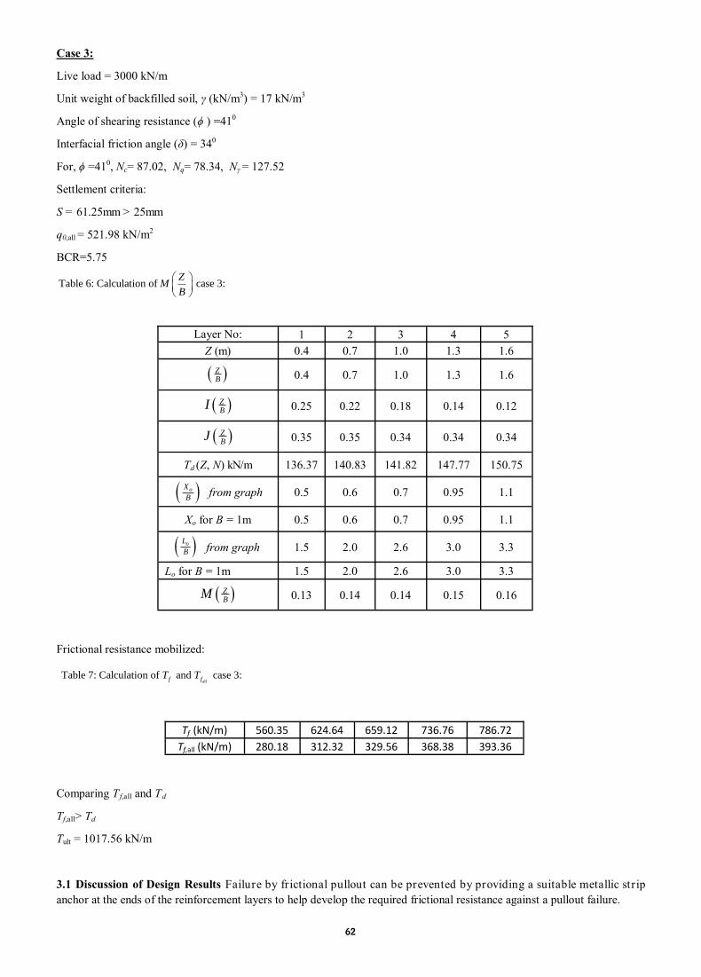
62
Case 3:
Live load = 3000 kN/m
Unit weight of backfilled soil, γ (kN/m3) = 17 kN/m3
Angle of shearing resistance (ϕ ) =410
Interfacial friction angle (δ) = 340
For, ϕ =410, Nc= 87.02, Nq= 78.34, Nγ = 127.52
Settlement criteria:
S = 61.25mm > 25mm
q0,all = 521.98 kN/m2
BCR=5.75
Frictional resistance mobilized:
Comparing T f,all and Td
Tf,all> Td
Tult = 1017.56 kN/m
3.1 Discussion of Design Results Failure by frictional pullout can be prevented by providing a suitable metallic strip
anchor at the ends of the reinforcement layers to help develop the required frictional resistance against a pullout failure.
allTable 7: Calculation of an ca :d se 3f fT T
Table 6: Calculation case 3f :oZ
MB
Layer No: 1 2 3 4 5
Z (m) 0.4 0.7 1.0 1.3 1.6
Z
B 0.4 0.7 1.0 1.3 1.6
Z
BI 0.25 0.22 0.18 0.14 0.12
Z
BJ 0.35 0.35 0.34 0.34 0.34
Td (Z, N) kN/m 136.37 140.83 141.82 147.77 150.75
from graph 0.5 0.6 0.7 0.95 1.1
Xo for B = 1m 0.5 0.6 0.7 0.95 1.1
from graph 1.5 2.0 2.6 3.0 3.3
Lo for B = 1m 1.5 2.0 2.6 3.0 3.3
Z
BM 0.13 0.14 0.14 0.15 0.16
oX
B
oL
B
Tf (kN/m) 560.35 624.64 659.12 736.76 786.72
Tf,all (kN/m) 280.18 312.32 329.56 368.38 393.36

63
By referring to the paper by Krishnaswamy and Mageshnagarajan in proceedings on National symposium on advances in
Geotechnical engineering NSAGE – 2004, it is presented when end anchors are not provided to the reinforcement, slight
increase in bearing capacity ratio was observed depending on the length of reinforcement and the point of maximum shear
stress. When anchors are provided, there is a dramatic increase in the bearing capacity ratio, depending on the passive
resistance developed across the anchor. The passive resistance of a reinforced earth bed can be improved by providing
anchors
There will be considerable saving of cost if we provide strip footing rather than raft foundation.
The worthiness of the recycled polymeric bag fabrics to be used for reinforcement purposes in reinforced earth bed was
confirmed.
The prohibitive cost of commercially available Geotextiles in India can be overcome by the extensive use of discarded
and used polymeric bags. The discarded and used polymeric bags can be joined together either by stitching or by epoxy
bonding and the same can be used as an alternative component instead of commercially available Geotextiles.
If the above mentioned recommendations are effectively implemented, it will significantly bring down the degree of
pollution caused by the indiscriminate discarding of plastic wastes.
1. Binquet, J. and Lee, K.L. (1975), “Bearing Capacity Analysis of Reinforced Earth Slabs”, Geotech. Engg. Divn, ASCE
101.
2. Krishnaswamy N.R.1, Shesha Prakash M.N.2, Deepak R.3, “Use of Poltmeric-Fabric waste in road construction”,
IJETCAS.
3. Raghavendra, H.B., Sitharam, T.G. and Murthy, B.R.S. (1998) Simplified approach to the analysis of a reinforced soil
bed as two-layer soil system. Journal of Ground Improvement.
4. Krishnaswamy, N.R. and Mageshnagarajan, M, (2004a). Circular and Strip footings on reinforced soil with anchors,
Proceedings of National Symposium on Advances in Geotechnical Engineering, Department of Civil Engineering,
Indian Institute of Science, Bangalore (NSAGE – 2004), July 22-23, pp. 163-168
5. Krishnaswamy, N.R. and Mageshnagarajan, M, (2004b). Reinforced soil – Foundation systems with Anchors,
Proceedings of International Conference on Geosynthetics and Geoenvironmental Engineering, Department of Civil
Engineering, Indian Institute of Technology Bombay, Mumbai (ICGGE – 2004), December 8-10, pp. 273-278.
4. CONCLUSION
REFERENCES

64
A STUDY ON BLUE BRAIN
Saloni Varshney* Department of Engineering,
Amity University, Gurgaon, Haryana, India
Email- [email protected]
*Corresponding author
Pooja Batra Nagpal Department of Engineering,
Amity University, Gurgaon, Haryana, India
Email- [email protected]
Human brain plays a pivotal role with the help of which the world is developing and considered intelligent. It is not possible
to model a brain and to upload the information of the natural brain into it. Think about the achievements that would be back
if we will be able to restore the brain of the greatest persons like Einstein or Mahatma Gandhi. Considering this, scientists
mentioned the world’s first virtual brain as “Blue Brain”. The scientists are researching for creating the virtual brain which
can response, take decision, think and can keep every data in the memory. The motive of the project is to preserve the brain
after the death so the data, feelings, memory and intelligence of that person would not lost. This paper presents the complete
research of blue brain including the concepts and functions.
Keywords: Brain; Neurons sensory Blue brain; artificial system.
Human brain is contemplated as the biggest gift that God has given to this world. Man is considered to be the most
intelligent because of his abilities that brain deliver him. The brain enables a person to respond by converting the
information transmitted by impulses. Technology is growing faster and faster. Virtual brain is an artificial brain, which is
able to respond, think and act as a real brain. This possibility can be turned into realization by using a super computer,
having large storage capacity and an interface between the human brain and the virtual brain. This interface helps to upload
the real brain into the virtual one. So the brain of any person along with its intelligence, knowledge and memory can be kept
and used even after death. One can also overcome the problems dealt in memorizing things such as important dates, roads
and routes, birthdays, history, etc. Even It is very difficult to understand the complexity of human brain. But now it is
possible to create a human brain. The project Blue Brain is under process for uploading human brain on supercomputer.
Henry Markram founded the project in May 2005 at the EPFL ( Ecole Polytechnique Federal De Lausanne ) in Lausanne,
Switzerland[2]. The Goal of the project is to achieve a complete understanding of the human brain and to enable faster and
better development of brain diseases. Data is gathered for about many neuron types which is used to build realistic models
of neurons. IBM created a Blue Gene supercomputer named “Blue Brain” to carry the simulations.
ABSTRACT
1. INTRODUCTION

65
The primary step is to gather information about all wide range of neuron types. This information is utilized to completely
study biology practical models of neuron and network of neurons. The simulations are completed by IBM on a Blue Gene
supercomputer [5]. Let us begin with the function of normal brain:-
I. Sensory input:
Initially, when our hands touch a warm surface, the neurons, communicate specific straight to the cerebrum. This activity of
getting data from environment is called sensory input.
II. Integration:
The understanding of things we have tasted, felt and touched which the body perceives into responses through neurons is
called integration.
III. Major output:
Once the brain learn, either by touching or tasting, at that point our mind communicates specific through neurons to effecter
cells, which really work to play out our solicitations with the help of which we see, listen, smell and feel.
I. Collection of Data:
It actually involves understanding the electrical behaviour of neurons by collecting the brain portion and analysing them
under a microscope. The observations obtained are then transformed into algorithm which becomes further ready for the
simulation process.
II. Simulation of Data:
There are two aspects of simulation:
(i). Speed of simulation
(ii). Simulation workflow
Speed of simulation: In 2012 simulation of one cortical column which consist of 10000 neurons run approximately 300
times slower than the real time. Accordingly one second of simulated time took about five minutes to complete. Now the
speed of simulation of one neocortical column is two hundred times slower than the real time. These simulations show
approximately linear scaling, that results in doubling the size of the neural network which doubles the time it takes to
simulate[9]. At present the primary goal is to gain biological validity instead of performance.
Simulation workflow: BBP-SDK (Blue Brain-SDK)is an open source software which uses C++, C, FORTAN. Moore
and Hines developed it in 1990’s. The BBP-SDK is a C++ wrapped in Python and Java[3]. Neural simulation is basically
used for building and using computational models of neurons. For blue brain, the current version of neuron which is in use
is 7.2.
III. Visualization:
RT Neuron is used for the visualisation of neural simulations. This software is generally written in C++ and OpenGL
[3]. This gives the 3D output. The initial phase was completed in December 2006, which included the simulation of the rat
neocortical column which are the small functioning units of neocortex which is usually responsible for conscious thoughts.
It is about 2 mm tall, having a diameter of 0.5 mm and contains 10,000 neurons in rats but in human it contains 60,000
neurons[1].
2. WORKING OF REAL BRAIN
3. FUNCTIONING OF BLUEBRAIN

66
I. Blue Gene Supercomputer:
The primary machine used for the project is a Blue Gene Supercomputer built by IBM.
a) BLUE GENE/L: IBM in June 2005 agreed to supply EPFL a “technology demonstrator” with the help of Blue Gene/L.
b) BLUE GENE/P: This supercomputer was upgraded to a Blue Gene/P in June 2010 in Lausanne with the following
specifications:-
1. Total: 16 terabytes of memory, 56 teraflops
2. GPFS parallel file system
3. Operating system: Linux SUSE SLE10
4. 1 PB of disk space
5. Silicon graphics: A 32-processor Silicon graphics Inc. (SGI) system is used for visualization of results with 300 GB of
shared memory [10].
6. Commodity PC clusters: Clusters of commodity PC’s have been used for visualization tasks with RT Neuron software.
REAL BRAIN BLUE BRAIN 1. SENSING PART
The neurons help in passing the message. The sensory
cell receives the input which produces electric impuls-
es. The impulses are received by neurons then trans-
ferred to the brain.
1. SENSING PART
In the Blue brain these sensory cell have been re-
placed by Silicon chip. It has been tested that these
neurons can produce electric impulse.
2.INTERPRETATION
The electric impulses are illustrated in the brain by
means of certain states of many neurons.
2. INTERPRETATION
The electric impulses are illustrated in the Blue brain
by means of registers. There are different values in the
register which represent the different states of brain.
3. RESULT
The brain sends the electric impulses representing the
responses which are further received by sensory cells
to respond neurons in the brain at that time.
3. RESULT
Based on the different states of register the brain send
the electric impulse representing the responses which
are further received by a particular register to respond
neurons at that time.
4. MEMORY
Certain neurons in the brain represent the states per-
manently. When required, the state is visualized by
our brain and we can easily remember the past things.
4. MEMORY
In the similar way the required state of registers can
be stored permanently and when required the infor-
mation can be received and used. 5.WORKING
Whenever we take decisions or make any computa-
tion, the computation are done in neural circuitry. The
past experiences stored and the inputs received are
used for the output.
5. WORKING
The decisions in virtual brain are taken by some
stored registers and the current inputs received for the
output.
4. COMPARISION OF REAL BRAIN AND BLUE BRAIN
5. BLUEBRAIN COMPONENTS

67
II. Blue Gene/Q:
JUQUEEN is an IBM Blue Gene/Q supercomputer. It was installed in May 2012 at the JULICH Research Centre in
Germany that currently performs at 1.6 pet flops and in June 2012 was ranked the world’s 8th fastest supercomputer. The
goal is to develop a three-dimensional model of the human brain[11].
III. Brain chip:
Brain chip was designed to provide a balance between durability, safety and functionality by Matthew Nagle. The chip had
to be small enough to not halt normal brain functions[3]. The chip recorded brain signals using integrated CMOS circuitry,
which is an array of recording electrodes[1]. The reliability of recorded data was improved by repeating experiments and
using multiple electrodes
i. Interpretation of electric impulse from the brain of animals can be helpful in understanding their thoughts.
ii. Even after the death of person his/her intelligence can be used for development.
iii. Things can be remembered without any effort.
iv. It would be possible to hear deaf people via direct nerve stimulation.
v. The decisions can be conducted without the actual presence of the person.
i. Supercomputers use a large amount of power.
ii. Human will become more dependent on machine.
iii. If the neural schema of person is hacked which will be uploaded on blue brain, it could be misused[7].
iv. There are threats of malware and viruses.
i. To discover Drug for brain disorder.
ii. Gathering and testing of 100 years of data.
iii. Cracking of neural code can be done.
iv. Brain simulation can be studied.
v. It can provide aid in relieving from conditions like depression, anxiety, stress and other genetic disorders[8].
vi. Social issues like various crimes, drug abuse can go eradicated.
Human brain is a pivotal part of human body and in near future we will be able to scan ourselves in the computer. The Blue
brain is the concept of reverse engineering having great benefits for humans. The serious threat is the combination of
biological and digital technologies. Despite all the difficulties, the project is aimed to be completed by 2023.
6. ADVANTAGES
7. DISADVANTAGES
8. APPLICATIONS
9. CONCLUSION

68
1. The Blue brain project, Hil, sean: Markram Henry, International conference of IEEE 2008.
2. Özkural E., What is it like to be a brain simulation?, Artificial General Intelligence. Springer Berlin Heidelberg, 232-
241(2012)
3. Henry Markram, "The Blue Brain Project", Nature Reviews Neuroscience, 7: 153- 160, 2006 February. PMID
16429124.
4. http://www.artificialbrains.com/blue-brain-project.
5. https://bluebrain.epfl.ch/Bluebrain
6. http://artificialbrains.com/blue-brain
7. http://www.neuron.yale.edu/neuron/
8. http://www.ncbi.nlm.nih.gov/pubmed/1642924
9. https://krazytech.com/blue-brain
10. http://www.forbes.com/technology/sciences/2005/06/06/cx_mh_0606ibm.html.
11. Nagal D. and Sharma S., An Overview On Discovery Of Reality-Blue Brain, (2013)
12. Schwartz Jeffrey M. and Sharon Begley, The mind and the brain. Harper Collins (2009)
REFERENCES

69
1. SCOPE OF THE JOURNAL
2. RPOSE OF HE JOURNAL
3. AIM OF THE JOURNAL
4. GUIDELINES FOR AUTHORS
INTERNATIONAL OF SCIENCES AND MANAGEMENT
(ISSN:
International Journal of Engineering, Sciences and Management is a bi-annual
journal of Dronacharya Group of Institutions, Greater Noida, UP, India.
To publish full-length research papers in any one or more of the following disciplines:
Computer Science & Engineering, Information Technology, Electrical, Electronics & Communication Engineering,
Mechanical Engineering, Civil Engineering, Physics, Mathematics, Economics, and Management.
To keep the academic community abreast of the research and technical scenario in the stated disciplines in the world.
The aim of the Journal is to percolate latest information in the fields of Engineering, Technology and Management to
aspiring minds to carryout meaningful research work and thereby benefit mankind in all possible ways. Knowledge shared
on this common platform will immensely help researchers for gainful outputs.
SUBMISSION OF MANUSCRIPTS: Soft copy of the manuscript for consideration of publication should be sent (as MS
Word Windows 2007 attachment) by Email to the Executive Editor at advisor.r&[email protected]
All papers, received for consideration of publication and complying with the below-mentioned format will be sent for
review to at least two referees. In accepting the paper for publication, the Editors and reviewers will give special weight to
readability and interest value for a wide readership besides the originality and the high-standard of its contents. The
Executive Editor’s decision is final in case of non-unanimity of opinion of referees. Under normal circumstances, the
authors will be informed about the status of their papers by the Executive Editor within eight weeks of their submission.
PREPARATION OF MANUSCRIPTS:
Manuscript: Manuscript should be in English, the preferred spelling being that of the Concise Oxford
Dictionary. It should be in ‘Times New Roman’, single-spaced, and typed on 8.5" x 11" or A4-size paper with
margins of 1" (25 mm) on each side. Manuscript should be typed in single column only (and not in double or triple
columns).

70
Title of Paper: Font size 16, ALL CAPITALS, bold, centered, and not underlined. The title must be 12.5 mm
below the top of the page (in addition to the standard 25 mm margin). The Title should adequately describe the
contents of the paper
Full names of all Authors, with * as superscript with corresponding author's name and his/her Email ID
(Font size 12, centered) and also the contact number. A blank line should be left between the title and the author's
name(s).
Full postal address along with affiliations (Font size 10, centered).
Abstract (Font size 10, centered) All papers must have a non-mathematical abstract of not more than 200 words.
The abstract should indicate the general scope of the paper, the important findings and the conclusions drawn.
The abstract should include only text. It should be specific about the methodologies used and the conclusion
drawn of the work reported. Please avoid the use of abbreviations and references. (Text of the Abstract: Font
size 9, single-space, justified).
Keywords: Include up to six keywords that describe your paper for indexing and for web searches. The more
discriminating your keywords are, the greater is the likelihood that your article will be found and cited. (Font size 9,
italics, left-justified).
Text: (Font size 10, Justified). The paper must be divided into sections starting preferably with "Introduction"
and ending with ''Conclusion". The main sections should be numbered 1, 2, 3 etc and subsections as 2.1, 2.2 etc.
Main headings should be typed in capitals, subheadings in lower case. Both types of heading should be underlined
and left-justified. Footnotes should be avoided. Equations should be typewritten and with the equation number
placed in parentheses at the right margin. Reference to the equation should use the form 'Eq. (3)'. Use extra line
spacing between equations, illustrations, figures and tables. The use of SI units is strongly recommended
Tables and Figures: Tables and Figures should be integrated with the text (and not sent separately at the end
of the manuscript) and numbered consecutively in the order in which reference is made to them in the text of
the paper. All captions must be centrally located above a Table and below a Figure (Font size 10). All tables and
figures must be numbered consecutively in Arabic numerals (not Roman) (e.g., Table 3 or Fig. 3) in the order of
appearance in the text. Tables & Figures should be reproduced in the exact format and at the exact place as desired
to appear in the journal.
Conclusion: A conclusion section must be included and should indicate clearly the advantages,
limitations and possible applications of the paper. Authors may also discuss about the scope of future work.
Acknowledgements: An acknowledgement section may be included after the ‘Conclusion’.
References: It is mandatory for references to be quoted in the text and be placed at the end of the text. They should
be numbered consecutively in order of their citation in the text and be indicated by superscripts in the text of the
manuscript. Examples of different citations as References are given below:
(i) In case of referring to an Article in a Journal
Kuebel, D.; Lahiri, M. & Wolf, E. An Inverse Problem in the Theory of Stochastic Electromagnetic Beams, Opt.
Commn., 282, 2009, p.141.
(ii) In case of referring to a Book/Monograph
Rao, C.N.R. & Raveau, B. (Eds.). Transition Metal Oxides, Wiley-VCH, 2nd Edition, 1998, Ch. 2.
(iii) In case of referring to a Conference Paper
Ctvrtnickova, T.; Mateo, M; Yanez, A. & Nicolas, G. Characterization of Coal Fly Ash Components by Laser-
Induced Breakdown Spectroscopy. Presented at the Fifth International Conf. on Laser-Induced Breakdown
Spectroscopy, Berlin, Adlershof, Germany. Sep 22-26, 2008, CP-15, p. 67-68.

71
(iv) In case of referring to a Report
Marine, R.E. & Iliff, K.W. Application of Parameter Estimation to Aircraft Stability and Control. NASA, USA,
1986, Report No. NASA-RP-1168.
Papers quoting the LATEST references from the referred journals will be preferred for publication unless the
original contribution from the author/s is of a very high standard.
Authors must include in the covering e-mail that their paper has not been published/accepted/submitted for publication/
presentation to any other journal/ book/conference in any form and the work submitted by them is their own and original.
The same ‘Undertaking’ should also be attached, on a separate page, along with the manuscript. This ethical policy of the
Journal will be strictly adhered to.
Note: Manuscripts not in conformity with these ‘Guidelines’ will not be forwarded to the experts for review.
UNDERTAKING


BUT WE CAN BUILD OUR YOUTH FOR THE FUTURE
WE CAN NOT ALWAYS BUILD THE FUTURE FOR OUR YOUTH,
GROUP OF INSTITUTIONS
-Franklin D Roosevelt
Here We Build Your Future
B. TECH COURSES| |Computer Science & Engineering Electronics & Communication Engineering Electronics & Computer Engineering
Electrical & Electronics Engineering Mechanical Engineering Computer Science and Information Technology| |
Information Technology Civil Engineering|
POST GRADUATE COURSESMaster of Business Administration (MBA) Master of Computer Application (MCA)|
Campus: #27, Knowledge Park- III, Greater Noida (UP) Phone: 0120-2323851-58, 2322022 | Email: [email protected] India Council for Technical Education, New Delhi (India) Dr. A. P. J. Abdul Kalam Technical University, Lucknow (India)Approved by: | Affiliated To:
DRONACHARYA GROUP OF INSTITUTIONS

Approved by
All India Council for Technical Education, New Delhi (India)
Affiliated To:
Dr. A. P. J. Abdul Kalam Technical University, Lucknow (India)
Campus:
# 27, Knowledge Park-III, Greater Noida (U.P.) – 201308 (India)
Phone: 0120-2323854-58, 2322022, Email: advisor.r&[email protected]
Corporate Office:
76P, Part-III, Sector-5, Gurgaon, 122001, Haryana (India)
Phone: 0124-2251602, 2253144, Email: [email protected]
desi
gn: w
ww
.stu
dio1
-indi
a.co
m
IJESM SIGHTINGS
www.dronacharya.info
J O U R N A L M A S T E R L I S T
Brazil 3.2%2.4%
India 60.0%
United States 13.2%
139 different countries have visited this site. 189 flags collected.
1.9%
1.1%
0.9%
0.8%
0.7%
0.7%
0.7%
0.5%
China
Unknown - A/P
Czech Republic
Malaysia
Nigeria
Pakistan
United Kingdom
Italy
0.9%Iran
1.0%Indonesia
Egypt
Others 11.8%


![Untitled-1 [files.cluster2.hostgator.co.in]files.cluster2.hostgator.co.in/hostgator103813/file/dgi...Processors AM3358 1GHz ARM Cortex-A8 processor TI AM3358 Sitara Processor Pipelining](https://img.pdfslide.us/doc/110x75/5fa46f15d24acd25ea7584f2/untitled-1-files-files-processors-am3358-1ghz-arm-cortex-a8-processor-ti.jpg)