Embed Size (px)
Citation preview

16
Available online at http://ijdea.srbiau.ac.ir
Int. J. Data Envelopment Analysis (ISSN 2345-458X) Vol. 1, No. 2, Year 2013 Article ID IJDEA-00122, 13 pages
Research Article
Finding a suitable benchmark for commercial
bank branches using DEA
M.R.Mozaffari*, F.hosseinzadeh Lotfi b, J.Gerami a
(a) Department of Mathematics, Science and Research Branch,Islamic Azad University,Fars, Iran
(b) Department of Mathematics, Science and Research Branch,Islamic Azad University,Tehran, Iran
Abstract
This paper proposes a suitable benchmark for inefficient commercial bank branches by using Data
Envelopment Analysis (DEA). In order to render an inefficient bank branch efficient, it is necessary to
decrease inputs and increase outputs. As there are priorities for decreasing some certain inputs and
increasing some certain outputs over other inputs and outputs, respectively, it is necessary to consider
and incorporate the managers’ view regarding the priorities in the models which are applied. So, in
this paper, using the enhanced Russell model for an inefficient bank branch, we propose the decrease
in inputs and the increase in outputs, taking the managers’ priorities into account. Finally, in a
numerical example, we apply the proposed procedure to the authentic information from 30
commercial bank branches, to show the application of the procedure.
Keywords: Data Envelopment Analysis, Benchmark, Linear programming.
1 Introduction
Data Envelopment Analysis (DEA), by Charnes, Cooper and Rhodes [3], is a method for evaluating
the relative efficiency of comparable entities referred to as Decision Making Units (DMUs). DEA
forms a production possibility frontier, or an efficient surface. If a DMU lies on the surface, i.e., there
is no other DMU that can either produce the same outputs by consuming less inputs (input-oriented
DEA) or produce more outputs by consuming the same amount of inputs (output-oriented DEA), it is
referred to as an efficient unit, otherwise inefficient. DEA also provides efficiency scores and
reference units for inefficient DMUs. The efficiency score tells the percentage by which a DMU
should decrease its inputs (input-oriented DEA) or increase its outputs (output oriented DEA) in order
to become efficient. Reference units are hypothetical units on the efficient surface, which can be
regarded as target units for inefficient units. In the traditional DEA, they are obtained by projecting an
inefficient DMU radially onto the efficient surface. The production theoretical argument for this
principle is that the DMU preserves its current input-output mix. However, from a managerial point of
* Corresponding author, Email address: [email protected], Tel:(+98728)4692104
International Journal of Data Envelopment Analysis Science and Research Branch (IAU)

62 M.R.Mozaffari, et al /IJDEA Vol. 1, No. 2 (2013) 61-73
view, it is possible that some other solution on the efficient surface might be a more preferable target,
i.e., there exists an input-output mix that is more suitable for the inefficient unit than the one obtained
through radial projection. One line of research in DEA concentrates on finding these targets for
inefficient DMUs (Golany [6], Thanassoulis and Dyson [11] and Zhu [12]). The DMU can use the
targets as goals or benchmarking units when working its way toward efficiency.
In Golany [6], a set of hypothetical reference units is generated and presented to the DMU. The DMU
may choose one of them as a target, or new reference units may be generated. In Thanassoulis and
Dyson [11], the DMU may articulate its preferences as a set of preference weights over improvements
for different input-output levels, or as an ideal target (neither necessarily optimal nor feasible ). The
target corresponding to the preference weights or the ideal target is then calculated. In the model by
Zhu [12], the DMU articulates its preferences as weights reflecting the relative degree of desirability
of the potential adjustments of current input or output levels. One major problem with a radial
measure of technical efficiency is that it does not reflect all identifiable potential for increasing
outputs and reducing inputs.
In economics, the concept of efficiency is intimately related to the idea of Pareto optimality. An input-
output bundle is not Pareto optimal if there remains the possibility of any net increase in outputs or
net reduction in inputs. When positive output and input slacks are present at the optimal solution of a
CCR or BCC linear programming problem in DEA, the corresponding radial projection of an
observed input-output combination does not meet the criterion of Pareto optimality and should not
qualify as an efficient point. The nonradial Russell measure was proposed by Färe and Lovell [5].
Russell [9] pointed out that this measure fails to satisfy a number of desirable properties of an
efficiency measure.For further explanation, notice the following example. Consider the evaluation of
various branches of a commercial bank. We have the following inputs/outputs:
Inputs: number of employees in the branch, area of the branch building, operation costs and
equipment. Outputs: resources, granted loans, total revenue, services and customer satisfaction.
In the classic models CCR, BCC, revised Russell and SBM, in order to make an inefficient branch
efficient, we have to decrease all inputs and increase all outputs to project the DMU onto the efficient
frontier. In evaluating these branches, the management declares that the priority for making inefficient
branches efficient is to decrease costs and the number of employees, and to increase services and
customer satisfaction. To make it clear, as the first priority, they should try to project the branch onto
the strong efficiency frontier by decreasing costs and the number of employees, and increasing
services and customer satisfaction. Otherwise, on the second priority, they should cover the
weaknesses existing in the former stage by decreasing the equipment and the area of the branch
building, and increasing resources, granted loans, and total revenue. The importance of the matter is
that the equipment and the area of the branch building are of vital importance to the management, and
decreasing them may damage the banking process. Considering the fact that there are some
restrictions in collecting resources, granting loans, and earning revenues, the management has decided
to put them in the second priority.
This paper is organized as follows. Section 2 provides a brief overview of DEA methodology and
benchmarking. Section 3 proposes a modified model to incorporate the managers views in the
enhanced Russell model. Section 4 contains an application of the proposed model by a numerical
example for 30 bank branches. Section 5 provides the conclusion.

16 M.R.Mozaffari, et al /IJDEA Vol. 1, No. 2 (2013) 61-73
2 Preliminaries
Consider DMUsn with m inputs and s outputs. The input and output vectors of jDMU
),1,=( nj are t
sjjj
t
mjjj yyYxxX ),,(=,),,(= 11 where 0.0,0,0, jjjj YYXX
By using the variable returns to scale, convexity, and possibility postulates, the non-empty production
possibility set (PPS) is defined as follows:
.,1=0,1,=,,:),(=1=1=1=
njYYXXYXT jj
n
jjj
n
jjj
n
jv
By the above definition, the BCC model proposed by Banker et al. [1] is as follows:
=1 =1
=1
=1
=1
Min [ ]
. = , = 1, ,
= , = 1, ,
= 1
0, = 1, ,
0, = 1, ,
0, = 1, , .
m s
i r
i r
n
j ij i ip
j
n
j rj r rp
j
n
j
j
j
i
r
s s
S t x s x i m
y s y r s
j n
s i m
s r s
(1)
Clearly, the evaluated pDMU is efficient if and only if 1=
* and all slack variables in the optimal
solution are zero in problem (1). Koopmans [3] defined an input-output vector as technically efficient
if and only if increasing any output or decreasing any input is possible only by decreasing some other
output or increasing some other input, respectively. A nonradial Pareto-Koopmans measure of
technical efficiency for pDMU can be computed as follows:

64 M.R.Mozaffari, et al /IJDEA Vol. 1, No. 2 (2013) 61-73
=1
=1
=1
=1
=1
1
Min =1
. , = 1, ,
, = 1, ,
= 1
0, = 1, ,
1, = 1, ,
1, = 1, ,
m
i
i
s
r
r
n
j ij i ip
j
n
j rj r rp
j
n
j
j
j
i
r
m
s
S t x x i m
y y r s
j n
i m
r s
(2)
In model (2) we suppose that all inputs and outputs are of the same importance in determining the
efficiency. That is to say, the priority in increasing or decreasing the outputs or the inputs,
respectively, is the same for all inputs and outputs. If there are different importance for different
inputs/outputs, we can use the following objective function instead of objective function (2).
=1
=1
=1
=1
1
,1
m
i im i
ii
s
r rs r
rr
where i , r show the importance of i , r , respectively.
Definition1. A DMU is called the benchmark for an inefficient unit if the DMU is on the efficiency
frontier and its inputs are not greater than (less than or equal to) and its outputs are not less than those
of that unit.
DMUs can benefit from benchmarking for continuous development and creating appropriate
conditions. Benchmarking cannot generally be used to solve the problems in an organization, but it
can be employed to accept activities prior to introducing novel processes. Benchmarking is, therefore,
beyond comparison, as awareness of conditions increases willingness for change; Measures should be
taken only when an organization is ready for change, and in order for a unit to be a successful
benchmark, the necessary preparations must be carried out and appropriate conditions should be
brought about.
3 A modification to the enhanced Russell model
Suppose that the management wants to give absolute priority to group of inputs over other inputs to
decrease, and also to a group of outputs over others to increase, and reach the frontier. 1I and 2I are
indices of the input set that are of the first and second priority, respectively, for the manager to

16 M.R.Mozaffari, et al /IJDEA Vol. 1, No. 2 (2013) 61-73
decrease the inputs and 1O and 2O are indices of the output set that are of the first and second
priority, respectively, for the manager to increase the outputs. For this propose, suppose inputs and
outputs vectors of jDMU ),1,=( nj are as follows, respectively.
),,(=21
jIjIj XXX where 0,>jX qIpImII |=|,|=|},,{1,2,= 2121
),,(=21
jOjOj YYY where 0,>jY .|=|,|=|},,{1,2,= 2121 lOkOsOO
The model used in this form will be as follows:
1 2
1 2
1 2
=1
1 2
=1
=1
1 2
1( )
Min ( , ) =1
( )
. , (3)
,
= 1
0, = 1, ,
1,
i i
i I i I
e p p
r r
r O r O
n
j ij i ip
j
n
j rj r rp
j
n
j
j
j
i
MMp q
R X Y
MMk l
S t x x i I I
y y r O O
j n
i I I
1 21, .
rr O O
In model (3), M is a large number which is used to show the view of the manager in the objective
function. We can define eR as the ratio of input average efficiency to output average efficiency.
Therefore, we have:
input average efficiency ) (1
=*
2
*
1iIiiIi
MqMp
output average efficiency ) (1
=*
2
*
1rOrrOr
MlMk
Theorem 1. In each optimal solution of model (3) all input and output constraints are binding.
Proof. Let ),,,,(*
2
*
1
*
2
*
1
*
OOII be an optimal solution of the model (3). By contradiction, suppose
that there exists ,21 IIt such that tpttjj
n
jxx
**
1=< , hence, tpttjj
n
jxx =
*
1= and
.<*
tt We put ),,,,(2121
OOII is a feasible solution for model (3) such that
,=,=*
22
*
II ,=*
11OO tipiiiOO ,1,=,=,=
**
22 and
66 M.R.Mozaffari, et al /IJDEA Vol. 1, No. 2 (2013) 61-73
tp
tjj
n
j
tx
x*
1==
. We have
) (1
) (1
<
) (1
) (1
*
2
*
1
*
2
*
1
21
21
rOrrOr
iIiiIi
rOrrOr
iIiiIi
MlMk
MqMp
MlMk
MqMp
,
which is a contradiction. The proof is, therefore, completed.
Theorem 2. 1<0 eR .
Proof. First, to prove 1eR , it is obvious that ),,,,(2121
OOII is a feasible solution of (3) and
the objective function value for this solution is 1 , and regarding minimization we have .1eR Now,
to prove 0>eR , by 00,21 II 11,,
21 OO we have 0eR .
We have to show that 0.eR By contradiction, suppose 0=eR , therefore 0=0,=21
II and
in the input constraints we have 211=0,= IIixx ipiijj
n
j , so, for all 0=, jj .
Also, we have ,,=0 211=OOryy rprrjj
n
j in the output constraints. Regarding
the fact that all21
, OO are strictly positive, we must have for all 0=, rpyr , and this contradicts
the assumption.
Theorem 3. 1=eR if and only if pDMU being evaluated is Koopmans-efficient.
Proof. Suppose 1=eR . To prove that pDMU is Pareto efficient, i.e., it is not dominated by any
member in vT , by contradiction assume there is vTYX ),( such that ).,(),( pp YXYX
Therefore, there exists 0 such that ).,(),(1=1= ppjj
n
jjj
n
jYXYX
Thus, there exists
1 2 =1, <
n
j tj tpjt I I x x or there exists .>,
1=21 qpqjj
n
jyyOOq
Without loss of generality, suppose there exists ,<1=21 tptjj
n
jxxIIt so define
=1= < 1.
n
j tjj
t
tp
x
x
Set tiIIi
x
x
i
tp
tjj
n
j
t
,1,=,= 21
1=
.1,= 21 OOrr
Then ),,,,(2121
OOII is a feasible solution of the model and we have
1,<
) (1
) (1
21
2,
1
rOrrOr
iIiitiIi
MlMk
MqMp
which is contradiction.

16 M.R.Mozaffari, et al /IJDEA Vol. 1, No. 2 (2013) 61-73
Now, suppose that pDMU is Pareto efficient. To prove 1=eR , by contradiction assume .1eR By
Theorem 1, we must have 1<eR . We must have for all 1,, ii and for all 1,, rr there
exists *, < 1
tt or there exists 1.>,
*
Without loss of generality, assume that there exists 1.<,*
tt Thus we have
.1,,1, ,,, 21
*
21
*
21
**
1=21
**
1=OOrIIiOOryyIIixx rirprrjj
n
jipiijj
n
j
Considering 1,<*
t we have
.,, ,,, 21
**
1=
**
1=21
**
1=OOryyyxxxtiIIixxx rprprrjj
n
jtptpttjj
n
jipipiijj
n
j
That is to say, a point in vT has been found such that ),,(),(*
1=
*
1= ppjj
n
jjj
n
jYXYX
which implies that pDMU is not Pareto efficient, and this is a contradiction.
Theorem 4. eR is strongly monotonic in inputs and outputs.
Proof. Suppose that, in the evaluation of pDMU , ),,,,(
*
2
*
1
*
2
*
1
*
OOII is the optimal solution,
then we have .,=,,= 21
**
1=21
**
1=OOryyIIixx rprrjj
n
jipiijj
n
j
Now assume that we increase at least one of the inputs by a constant , say
0).>(= tptp xx
Consider the th
t input constrains ),(= **
1= tpttjj
n
jxx .1It
Suppose .)(
=
**
1,=
kx
xx
tp
tpptjj
n
pjj
t
Regarding ,
=
*
1=*
tp
tjj
n
j
tx
x
note that we
always have 1.*p Therefore, we have
.=
<)(
=*
*
1=
**
1,=
t
tp
tjj
n
j
tp
tpptjj
n
pjj
tx
x
x
xx
Therefore, by defining tiIiii ,,= 1
* , the solution ),,,,(*
2
*
1
*
21
*
OOII is a feasible
solution of DMU under evaluation , and we have
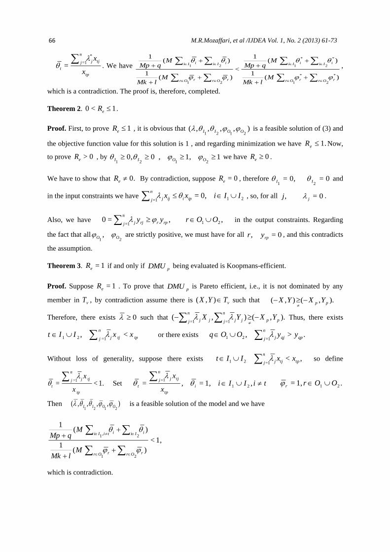
68 M.R.Mozaffari, et al /IJDEA Vol. 1, No. 2 (2013) 61-73
.
) (1
) (1
<
) (1
) (1
*
2
*
1
*
2
*
1
*
2
*
1
*
21
rOrrOr
iIiiIi
rOrrOr
iIiiIi
MlMk
MqMp
MlMk
MqMp
This show that eR is strictly decreasing with respect to the inputs of the DMU under
evaluation. It can be shown, in a similar manner, that eR is strictly increasing with respect to
the outputs of the DMU under evaluation.
Theorem 5. eR satisfies the following conditions:
(i) If (<)1> then )(),( ppe YXR
1).,( ppe YXR
(ii)If (>)1< then )(),( ppe YXR ).,( ppe YXR
Proof. (i) Suppose that ),,,,(*
2
*
1
*
2
*
1
*
OOII is the optimal solution in the evaluation of .pDMU
Then ),,1
,1
,(*
2
*
1
*
2
*
1
*
OOII
is a feasible solution in the evaluation of ),,( pp YX and we have
).,(1
=
) (1
)1
1
(1
),(*
2
*
1
*
2
*
1
ppe
rOrrOr
iIiiIi
ppe YXR
MlMk
MqMp
YXR
(ii) Suppose that ),,,,(*
2
*
1
*
2
*
1
*
OOII is the optimal solution in the evaluation of ),( pp YX . The, by
assuming )1
,1
,,,(*
2
*
1
*
2
*
1
*
OOII
is a feasible solution in the model evaluating pDMU , and we
have ).,(=
)1
1
(1
) (1
),(*
2
*
1
*
2
*
1
ppe
rOrrOr
iIiiIi
ppe YXR
MlMk
MqMp
YXR
Therefore, considering Theorem 1 and the above variable alteration in model (3), the SBM model is
modified to the following model :
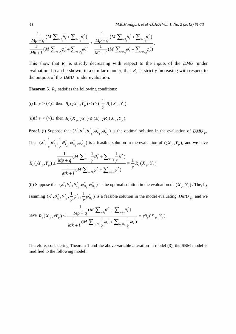
16 M.R.Mozaffari, et al /IJDEA Vol. 1, No. 2 (2013) 61-73
* 1 2
1 2
1 2
=1
1 2
=1
=1
1
11 ( )
11 ( )
. = ,
= ,
= 1
0, = 1, ,
0,
i i
i I i Iip ip
r r
r O r Orp rp
n
j ij i ip
j
n
j rj r rp
j
n
j
j
j
i
s sM
Mp q x xMin
s sM
Mk l y y
S t x s x i I I
y s y r O O
j n
s i I I
2
1 2 0, .
rs r O O
(4)
If Model (4) has multiple optimal solutions, there are several benchmarks for DMUp and more
choices of suitable benchmarks for the management to choose from. Therefore, in order to find the
multiple optimal solutions of Model (4), we solve it again after adding the constraint *
. It is
not, of course, possible to find all the alternative solutions; One can only determine the extreme
DMUs and find their convex combination as the desirable benchmark.
To solve Model (4), we obtain Model (5) by a change of variable, and then we transform the
fractional linear model to a linear programming model. Finally, we put the optimal solution of Model
(5) in *
*
*
*
*
*
*
*
*,,
r
r
i
i
j
j
ts
ts to obtain the optimal solutions and the desirable benchmark for
the DMUs.
70 M.R.Mozaffari, et al /IJDEA Vol. 1, No. 2 (2013) 61-73
1 2
1 2
1 2
=1
1 2
=1
=1
1
1Min ( )
1. ( ) = 1
= ,
= , (5)
=
0, = 1, ,
0,
i i
i I i Iip ip
r r
r O r Orp rp
n
j ij i ip
j
n
j rj r rp
j
n
j
j
j
i
t tM
Mp q x x
t tS t M
Mk l y y
x t x i I I
y t y r O O
j n
t i I
2
1 2 0,
0.
r
I
t r O O
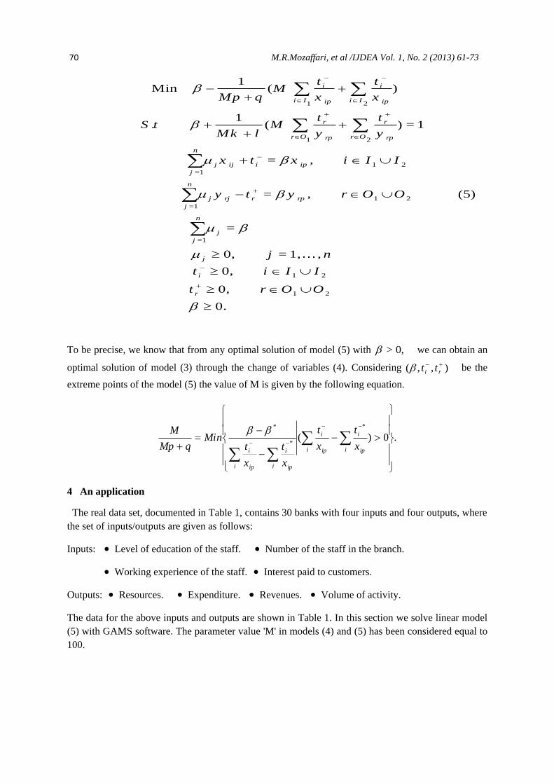
To be precise, we know that from any optimal solution of model (5) with ,0> we can obtain an
optimal solution of model (3) through the change of variables (4). Considering ),,(
ri tt be the
extreme points of the model (5) the value of M is given by the following equation.
.0)(
*
*
*
ip
i
iip
i
i
ip
i
iip
i
i
x
t
x
t
x
t
x
tMin
qMp
M
4 An application
The real data set, documented in Table 1, contains 30 banks with four inputs and four outputs, where
the set of inputs/outputs are given as follows:
Inputs: Level of education of the staff. Number of the staff in the branch.
Working experience of the staff. Interest paid to customers.
Outputs: Resources. Expenditure. Revenues. Volume of activity.
The data for the above inputs and outputs are shown in Table 1. In this section we solve linear model
(5) with GAMS software. The parameter value 'M' in models (4) and (5) has been considered equal to
100.

66 M.R.Mozaffari, et al /IJDEA Vol. 1, No. 2 (2013) 61-73
Table 1
Data contains 30 banks with four inputs and four outputs
DMUs 1i 2i 3i 4i 1o 2o 3o 4o
1 73504.25 86 4000 61196520.56 57029.55 40.88 1269 175
2 36582.75 89.77 2565 66287094.89 36872 18.55 8543.33 313.11
3 25002.25 87 1343 47612874.67 38680 20.22 6594.77 274.88
4 36684.75 94 1500 349278138.6 35933 32.44 10516.55 248.55
5 36834.5 83.44 1680 68356757.22 54457.77 30.11 9684.66 221.66
6 62611.62 97 3750 75508661.33 72277.11 11.77 8022 329
7 41572.77 90.66 3313 114264317.2 36625.44 101.22 14513.33 264.66
8 55949.62 92 1500 74950922.22 46360.33 17.11 1622.55 226.11
9 95522.75 89.55 1600 106720450.6 86063.33 71.44 10645 297.88
10 59080.62 95.22 1725 66010355.44 47242.11 26.22 6824.33 215.77
11 40736.12 78.33 1920 86613046.78 38977.77 184.11 12226 178.33
12 27300.62 89.66 4433 69942333.33 38214.88 21.77 7561.77 157.44
13 63295 106.33 2500 78657408.78 58340.44 45.22 7584 269.55
14 94969.87 93.77 2800 78951533.89 88472.33 40 661.22 136.22
15 50062 93.44 1630 69126959.33 50499 14.33 10264.11 125.11
16 45926.25 85 1127 146206909 47907.22 25 7491.55 188.55
17 82202.5 104 3400 107289969.8 59579.77 19.88 4952.77 157.33
18 88782.5 92.33 1304 165532950.4 83075.11 23.44 4917 141.55
19 87247.25 96.11 4206 68355245.33 51026.55 17.55 1528.33 217.77
20 33196.5 100.44 1340 92342642.33 29658.11 77.33 14766.33 306.22
21 28402.75 89.33 1393 44055007.78 27735 19.22 940.66 165.11
22 122897.87 121.88 2191 94312914.11 102855.11 47.55 2510.44 238
23 32587.75 100 2140 89070348.78 34063.66 23.11 2110.88 349
24 60866.37 92 1231 69549538.56 53731.33 63.33 10219.55 163.55
25 86429.87 90 1960 164581079.9 75776.55 53.88 4480.33 253.44
26 253690 890 13430 694238180 1000 3 650 27
27 1002200 920 16000 1829518580 9000 17 164 29
28 66803.12 93.55 1603 143921177.8 72552.66 75.88 12091.22 184.77
29 40156.12 82.33 2300 65099487.67 38630.77 24.88 1460.55 75.33
30 986780 950 13040 3891855920 1800 7 491 14
Now in Table 1, the suitable index for inefficient branches can be suggested by considering the
priority of decreasing 21, ii and 3i and also priority of increasing 3o and 4o .
( {1,2}={3,4},={4},={1,2,3},= 2121 OOII ). Therefore, we calculate optimal values in order to
evaluate the bank branches by model (5). Then considering the change of variables, the optimal
solution of model (4) will be obtained. We put the optimal value of model (4) in the Table

72 M.R.Mozaffari, et al /IJDEA Vol. 1, No. 2 (2013) 61-73
Table 2
Benchmarks for each branch by using the proposed approach.
The results of Model (4) are provided in Table 2. The set of inefficient units is denoted by IN; For the
data in Table 1, this set is
.,,,,,,,,, 302726251917131284 DMUDMUDMUDMUDMUDMUDMUDMUDMUDMUIN
By Model (4) and the results of Table 2, the desirable benchmark for 4DMU is obtained from the
convex combination of units 5, 7, 9, 11, and 20; and for 8DMU it is obtained from the convex
combination of units 3, 5, 20 and 24. Moreover, 20DMU is a good benchmark for units 26, 27, and
30. Looking more closely at the inputs and outputs of 30DMU , one can observe that the necessary
amount of decrease for inputs 1-3, which have higher priority, is 0.03, 0.11, and 0.10, respectively,
and the decrease required for input 4 to reach 20DMU is 0.2.
DMUs 1i 2i 3i 4i 1o 2o 3o 4o
1 73504.25 86.00 4000.00 6.11965E+7 57029.56 40.89 1269.00 175.00
2 36582.75 89.78 2565.00 6.62871E+7 36872.00 18.56 8543.33 313.11
3 25002.25 87.00 1343.00 4.76129E+7 38680.00 20.22 6594.78 274.89
4 36684.75 94.00 1500.00 8.87670E+7 35933.00 90.82 13564.99 272.14
5 36834.50 83.44 1680.00 6.83568E+7 54457.78 30.11 9684.67 221.67
6 62611.63 97.00 3750.00 7.55087E+7 72277.11 11.78 8022.00 329.00
7 41572.77 90.67 3313.00 1.14264E+8 36625.44 101.22 14513.33 264.67
8 38851.85 89.92 1500.00 7.49509E+7 46360.33 48.76 11170.70 240.34
9 95522.75 89.56 1600.00 1.06720E+8 86063.33 71.44 10645.00 297.89
10 39697.81 91.10 1725.00 6.60104E+7 47242.11 34.57 8676.21 290.85
11 40736.13 78.33 1920.00 8.66130E+7 38977.78 184.11 12226.00 178.33
12 27300.63 89.35 1408.82 5.52739E+7 38214.89 28.79 7893.31 281.21
13 53669.46 93.60 2500.00 7.86574E+7 58340.44 45.22 9632.53 300.76
14 94969.88 93.78 2800.00 7.89515E+7 88472.33 40.00 661.22 136.22
15 50062.00 93.44 1630.00 6.91270E+7 50499.00 14.33 10264.11 125.11
16 45926.25 85.00 1127.00 1.46207E+8 47907.22 25.00 7491.56 188.56
17 66259.14 94.67 1477.92 0.99970E+8 59579.78 74.21 12580.06 301.80
18 88782.50 92.33 1304.00 1.65533E+8 83075.11 23.44 4917.00 141.56
19 35453.47 85.13 1621.83 6.83552E+7 51026.56 32.96 9804.68 233.31
20 33196.50 100.44 1340.00 9.23426E+7 29658.11 77.33 14766.33 306.22
21 8402.75 89.33 1393.00 4.40550E+7 27735.00 19.22 940.67 165.11
22 122897.88 121.89 2191.00 9.43129E+7 102855.11 47.56 2510.44 238.00
23 32587.75 100.00 140.00 8.90703E+7 34063.67 23.11 2110.89 349.00
24 60866.38 92.00 1231.00 6.95495E+7 53731.33 63.33 10219.56 163.56
25 84279.99 90.00 1907.35 1.07781E+8 75776.56 77.02 11443.43 292.00
26 33196.50 100.44 1340.00 9.23426E+7 29658.11 77.33 14766.33 306.22
27 33196.50 100.44 1340.00 9.23426E+7 29658.11 77.33 14766.33 306.22
28 66803.13 93.56 1603.00 1.43921E+8 72552.67 75.89 12091.22 184.78
29 40156.13 82.33 2300.00 6.50995E+7 38630.78 24.89 1460.56 75.33
30 33196.50 100.44 1340.00 9.23426E+7 29658.11 77.33 14766.33 306.22

66 M.R.Mozaffari, et al /IJDEA Vol. 1, No. 2 (2013) 61-73
5 Conclusion
The main nature of benchmarking is an attempt for improvement and its purpose is to provide
performance levels and a quantitative criterion for the results. In internal benchmarking, a DMU is
compared with another DMU within the organization, which leads to easier interactions, more
profound analyses, and clarification of problems. In this paper suggested a model using an modified
Russell to find a suitable index for inefficient commercial banks. The suggest model can introduce a
suitable efficient branch in order to give priority to decrease some inputs also to give priority to
increase some outputs. For practical application, the discretionary and nondiscretionary data can be
determined and also the suggest model can be studied in mentioned in order to eliminate the priorities
which are on the discretionary and nondiscretionary introduce the suitable and practical index.
References
[1] Banker ,R.D , Charnes A and Cooper W.W, 1984. Some models estimating technical and and scale inefficiencies in Data Envelopment Analysis. Management Science 30,1078-1092
[2] Charnes.A, Cooper. W.W. Programming with linear fractional functions, Naval Res. Logist.
Quart. 9, 181–186, 1962.
[3] Charnes, A., Cooper, W.W, Rhodes, E. Measuring the efficiency of decision making units.
European Journal of Operational Research 2, 429-444, 1978.
[4] Cooper W.W, Seiford, L, Tone, K. Data envelopment analysis a comprehensive text with Models
applications references , DEA solved software. Third Printing. By Kluwer academic publishers. 2002.
[5] Färe. R, and Lovell. C. A. K. Measuring the technical efficiency of production, J. Econ. Theory
19, 150-162, 1978.
[6] Golany, B. An Interactive MOLP Procedure for the Extension of DEA to Effectiveness Analysis,
Journal of Operational Research Society 39, 725-734, 1988.
[7] Koopmans, T.C. An analysis of production as an efficient combination of activities. In:
Koopmans, T.C. (Ed.), Activity Analysis of production and Allocation. Wiley ,New York. 1951
[8] Pastor. J.T, Ruiz .J.L, Sirvent. I. An enhanced DEA Russell graph efficiency measure . European
Journal of Operational Research , 115,569-607,1999.
[9] RUSSELL. R. R, Measures of technical efficiency, J. Econ. Theory 35, 109-126, 1985.
[10]Tone, K. A slack based measure of efficiency in data envelopment analysis. Research report,
Institute for Policy Science, Saitama University, August. 1997.
[11] Thanassoulis E. and Dyson R.G, 1992. Estimating preferred target input-output levels using Data
Envelopment Analysis. European Journal of Operational Research, 56, 80-97, 1985.
[12] Zhu, J. Data Envelopment Analysis with Preference Structure, Journal of the Operational
ResearchSociety,47,136-150,199