K.7

International Dollar Flows Banegas, Ayelen, Ruth Judson, Charles Sims, and Viktors Stebunovs

International Finance Discussion Papers Board of Governors of the Federal Reserve System

Number 1144 September 2015

Please cite paper as: Banegas, Ayelen, Ruth Judson, Charles Sims, and Viktors Stebunovs (2015). International Dollar Flows. International Finance Discussion Papers 1144. http://dx.doi.org/10.17016/IFDP.2015.1144

Board of Governors of the Federal Reserve System

International Finance Discussion Papers

Number 1144

September 2015

International Dollar Flows

Ayelen Banegas

Ruth Judson

Charles Sims

Viktors Stebunovs

NOTE: International Finance and Discussion Papers are preliminary materials circulatedto stimulate discussion and critical comment. References in publications to InternationalFinance Discussion Papers (other than an acknowledgment that the writer has had access tounpublished material) should be cleared with the author or authors. Recent IDFPs are avail-able on the Web at www.federalreserve.gov/pubs/ifdp/. This paper can be downloadedwithout charge from Social Science Research Network electronic library at www.ssrn.com.

International Dollar Flows

Ayelen Banegas∗Ruth Judson#

Charles Sims†Viktors Stebunovs‡

Abstract: Using confidential Federal Reserve data, we study the factors driving U.S.banknote flows between the United States and other countries. These flows are a significantcomponent of capital flows in emerging market economies, where physical U.S. currencyfunctions as a safe asset and precautionary demand for U.S. banknotes is a form of flight toquality. Prior to the global financial crisis, country-specific factors, including local economicuncertainty, largely explain the volume and heterogeneity of the flows. Since the crisis, globalfactors, particularly, global economic uncertainty, explain the flows markedly well. Further,precautionary demand for U.S. banknotes is not episodic.

Keywords: capital flows, currency flows, U.S. banknotes, safe asset, emerging marketeconomies, economic uncertainty, flight to quality, capital flight, money demand.

JEL Classifications: F30; E40; E50.

∗ Board of Governors of the Federal Reserve System, 20th Street and Constitution Av-enue, NW, Washington, DC 20551, U.S.A.; maria.a.banegas@frb.gov. URL: http://www.federalreserve.gov/econresdata/ayelen-banegas.htm.# Board of Governors of the Federal Reserve System, 20th Street and Constitution Avenue,NW,Washington, DC 20551, U.S.A.; rjudson@frb.gov. URL: http://www.federalreserve.gov/econresdata/ruth-a-judson.htm.† Federal Reserve Bank of New York, 33 Liberty Street, New York, NY 10045, U.S.A.;charles.sims@ny.frb.org.‡ Board of Governors of the Federal Reserve System, 20th Street and Constitution Av-enue, NW, Washington, DC 20551, U.S.A.; viktors.stebunovs@frb.gov. URL: http://www.federalreserve.gov/econresdata/viktors-stebunovs.htm.The views in this paper are solely the responsibility of the authors and should not be in-terpreted as reflecting the views of the Board of Governors of the Federal Reserve Systemor of any other person associated with the Federal Reserve System. We are grateful forhelpful comments to Carol Bertaut, Nicholas Bloom, Neil Ericsson, Stijn Claessens, RichardPorter, Patrice Robitaille, staff at the Federal Reserve Bank of New York Cash and CustodyFunction, and participants of seminars at the Federal Reserve Board and the 2014 Interna-tional Cash Conference at the Deutsche Bundesbank. We thank Patrick Kennedy and CalebWroblewski for excellent research assistance.

1 Introduction

Demand for U.S. dollars is driven by both domestic and international developments.1

Like the banknotes in other advanced economies, U.S. dollars tend to be used domestically asa medium of exchange. But, unlike the banknotes of most other advanced economies, U.S.dollars are extensively used far beyond the country’s borders as a safe asset, particularlyin emerging market economies, where conventional safe assets are not available. Whilebanknotes are generally a small portion of cross-border financial flows—about 5 percent ofnet foreign private acquisitions of U.S. securities—for some countries in some years they canbe substantial. For example, over the last decade and a half, net shipments of U.S. dollarsto Argentina in some months exceeded a few percent of the country’s annual GDP. Morerecently, in 2014, euros and U.S. dollar banknote shipments to Russia amounted to about$50 billion, or about a third of the country’s net capital outflows that year. In this context,for an emerging market economy, elevated, precautionary demand for U.S. banknotes is aform of flight to quality by its residents, which contributes to a broader capital flight.

Indeed, prior to the global financial crisis, episodes of unusually high demand for U.S.dollars, identified by elevated U.S. currency outflows from the United States, appeared tocorrespond to periods of economic or political crisis in specific countries or regions—forexample, in Argentina or in the former Soviet Union. But, more recently, with the collapseof Lehman Brothers and the beginning of the global financial crisis, currency demand fromabroad turned up sharply and, in contrast to earlier years, became broad-based rather thancountry- or region-specific.

In this paper, we study the factors driving demand for U.S. banknotes from abroad. Weuse a confidential data set of currency shipments by commercial banks between the UnitedStates and other countries, which is complied by the Federal Reserve. Our data set coversmonthly payments and receipts—bilateral U.S. banknote flows between the United Statesand other countries—for a large number of countries from the mid-1990s to the present.2

Specifically, we analyze net shipments, defined as the difference between payments to andreceipts from a country, in aggregate and for various country groupings over the last decadeand a half.3 Net shipments cleanly identify demand for U.S. dollars because the supply of U.S.banknotes is perfectly elastic: The Federal Reserve supplies U.S. banknotes to commercialbanks in a requested amount on a short notice.4

1In this paper, “U.S. dollars” and “dollars” refers to physical banknotes rather than dollar-denominatedassets. The vast majority of U.S. dollar banknotes in circulation (currently, about $1.3 trillion, 11 percentof M2) are Federal Reserve notes.

2For example, net shipments are positive for a country that imports U.S. dollars and negative for acountry that exports U.S. dollars.

3Although this data set begins in the late 1980s, we focus on the period from January 2000 to June 2013because of limitations in data quality and coverage in the early part of the sample.

4Such a transaction also requires a payment of reserve balances to the Federal Reserve in the requestedamount. Effectively, this is an exchange of cash for reserve balances. Conversely, the Federal Reserve also

1

Building on the dollarization and capital flows literature, we explain net shipments withcountry-specific characteristics (past dollar use, local economic uncertainty, and local eco-nomic conditions) and global determinants (common shocks external to the country, suchas global economic uncertainty) over the pre- and post-crisis periods. Because we empha-size the function of the U.S. dollar as a safe asset, we construct measures of local economicuncertainty using financial data and several measures of global economic uncertainty, whichrely on financial market data and on Baker, Bloom, and Davis (2015) uncertainty indexesthat are derived from U.S. and European news sources.

For net shipments in aggregate, our findings are consistent with those in the capital flowsliterature discussing determinants of broader capital flows (for example, Fratzscher (2012),Forbes and Warnock (2012), and Ghosh, Qureshi, Kim, and Zalduendo (2014)). Specifically,our regression analysis of net shipments in aggregate suggests that global factors that captureboth financial risk and economic uncertainty predict U.S. banknote flows. In addition,these common factors have become increasingly important since the global financial crisis.While we rely on economic uncertainty indexes compiled from U.S. and European sources,we note that, by construction, they reflect U.S., European, and international events.5 Tofurther strengthen the point that global uncertainty matters, we use a common component ofeconomic uncertainty indexes for the United States and Europe in some regressions. Otherglobal variables—in particular, typical determinants of money demand—play only a smallrole. We find mixed evidence on the explanatory power of macroeconomic indicators, suchas global GDP growth and inflation.6 Overall, at the aggregate level, our regression analysesindicate that global factors can explain significant amounts of variation in currency flows.

For our analysis of net shipments to countries grouped by the level of economic devel-opment or by the patterns of currency flows, we rely on a Hausman and Taylor (1981)specification that allows for including both country fixed effects and time-invariant countrycharacteristics in a regression model. Our results also show that, since the global financialcrisis, global economic uncertainty has an increasingly important role in explaining dollarflows, particularly to emerging market economies. The results also suggest a greater sensi-tivity of demand from abroad for U.S. banknotes to changes in economic uncertainty relativeto changes in financial market stress. In addition, we find a large degree of heterogeneityacross countries, with local factors such as inflation and global factors such as economic un-certainty having a larger effect on demand for U.S. banknotes in emerging market economiesthan in advanced economies. We show that mostly global factors explain flows to countriesthat do not use U.S. dollars but distribute them to other, less-developed regions and coun-

buys U.S. banknotes from commercial banks and, in exchange, pays them in reserve balances.5Moreover, U.S. financial and economic developments may have international spillovers: For example, the

2013 taper tantrum resulted in substantial capital outflows from emerging market economies.6Our findings show that there is no significant relationship between currency flows and the broad U.S.

dollar index, oil prices, and gold prices.

2

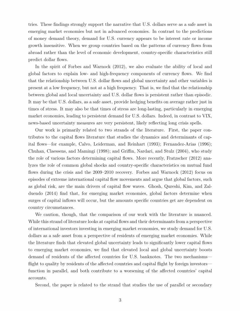
tries. These findings strongly support the narrative that U.S. dollars serve as a safe asset inemerging market economies but not in advanced economies. In contrast to the predictionsof money demand theory, demand for U.S. currency appears to be interest rate or incomegrowth insensitive. When we group countries based on the patterns of currency flows fromabroad rather than the level of economic development, country-specific characteristics stillpredict dollar flows.

In the spirit of Forbes and Warnock (2012), we also evaluate the ability of local andglobal factors to explain low- and high-frequency components of currency flows. We findthat the relationship between U.S. dollar flows and global uncertainty and other variables ispresent at a low frequency, but not at a high frequency. That is, we find that the relationshipbetween global and local uncertainty and U.S. dollar flows is persistent rather than episodic.It may be that U.S. dollars, as a safe asset, provide hedging benefits on average rather just intimes of stress. It may also be that times of stress are long-lasting, particularly in emergingmarket economies, leading to persistent demand for U.S. dollars. Indeed, in contrast to VIX,news-based uncertainty measures are very persistent, likely reflecting long crisis spells.

Our work is primarily related to two strands of the literature. First, the paper con-tributes to the capital flows literature that studies the dynamics and determinants of cap-ital flows—for example, Calvo, Leiderman, and Reinhart (1993); Fernandez-Arias (1996);Chuhan, Claessens, and Mamingi (1998); and Griffin, Nardari, and Stulz (2004), who studythe role of various factors determining capital flows. More recently, Fratzscher (2012) ana-lyzes the role of common global shocks and country-specific characteristics on mutual fundflows during the crisis and the 2009–2010 recovery. Forbes and Warnock (2012) focus onepisodes of extreme international capital flow movements and argue that global factors, suchas global risk, are the main drivers of capital flow waves. Ghosh, Qureshi, Kim, and Zal-duendo (2014) find that, for emerging market economies, global factors determine whensurges of capital inflows will occur, but the amounts specific countries get are dependent oncountry circumstances.

We caution, though, that the comparison of our work with the literature is nuanced.While this strand of literature looks at capital flows and their determinants from a perspectiveof international investors investing in emerging market economies, we study demand for U.S.dollars as a safe asset from a perspective of residents of emerging market economies. Whilethe literature finds that elevated global uncertainty leads to significantly lower capital flowsto emerging market economies, we find that elevated local and global uncertainty boostsdemand of residents of the affected countries for U.S. banknotes. The two mechanisms—flight to quality by residents of the affected countries and capital flight by foreign investors—function in parallel, and both contribute to a worsening of the affected countries’ capitalaccounts.

Second, the paper is related to the strand that studies the use of parallel or secondary

3

currencies and constructs estimates of external U.S. dollar and euro circulation. Kamin andEricsson (2003) is an example of the former and Judson (2012) of the latter.7 This strandof literature, however, does not explicitly recognize that the U.S. dollars functions as a safeasset in emerging market economies.

Our analysis has important implications for policy makers. From the perspective offoreign central banks, particularly those in emerging market economies, elevated demand forU.S. dollars is a form of flight to quality (by residents of these countries) that may result insubstantial loss of official foreign exchange reserves. Hence, understanding and quantifyingthe factors affecting such demand is crucial for foreign central banks’ operations, includingdetermining a desired size of foreign exchange reserves. In this context, our novel findingsis the increasing importance of global factors as determinants of currency flows for a givencountry.8

The remainder of this paper proceeds as follows. In the next section, we place our workin the context of previous studies on international capital flows and external U.S. dollarusage. In Section 3, we review the primary data sources and highlight some challenges ofmeasuring international dollar flows. In Section 4, we present results for our set of aggregateregressions on the links between global factors and global demand for U.S. currency. InSection 5, we present results for our panel regressions and evaluate the ability of both globaland country-specific factors to explain international currency flow dynamics. In Section 6,we present a very brief overview of the significance of currency for Federal Reserve operationsand policy making (and, in Appendix C, we construct a hypothetical estimate the effectsof various trajectories for currency growth on the implementation of U.S. monetary policy).The final section concludes and provides some direction for future research.

2 Place in the literature

Currency flow data are highly confidential and are therefore largely unexplored in theliterature, even though these flows are a significant component of capital flows for somecountries. Hence, we rely mainly on two literature strands—on broader capital flows and oncurrency substitution—that appear related to our topic.

First, the paper contributes to the capital flows literature that studies the dynamics anddeterminants of capital flows. We build on previous work by Calvo, Leiderman, and Reinhart(1993), Fernandez-Arias (1996), Chuhan, Claessens, and Mamingi (1998), Griffin, Nardari,

7Other empirical studies include Doyle (2000), Judson and Porter (1996), Stix (2010), Fischer, Kohler,and Seitz (2004), Bartzsch, Rosl, and Seitz (2013), and Hellerstein and Ryan (2011), who use a portion ofour data over an earlier period.

8Understanding the factors driving demand from abroad for U.S. dollars—a major contributor to U.S.currency growth—is also important for a wide range of Federal Reserve operational considerations and forthe normalization of monetary policy, including potential large-scale liquidity draining operations and salesof securities from the Federal Reserve’s System Open Market Account portfolio.

4

and Stulz (2004) that study the role of various factors determining capital flows.9 Morerecently, Fratzscher (2012) analyzes the role of common global shocks (push factors) andcountry-specific characteristics (pull factors) on global portfolio flows during the crisis andthe 2009–2010 recovery. He finds that push factors such as global risk and liquidity had a sig-nificant effect on mutual fund flow dynamics, and that pull factors, including macroeconomicfundamentals, country risk, and institutional quality, can help explain the heterogeneity ofportfolio flows across countries. Forbes and Warnock (2012) focus on episodes of extremeinternational capital flow movements—surges, stops, flights, and retrenchments—and arguethat global factors, such as global risk, are the main drivers of capital-flow waves. Theyexamine both capital inflows and outflows and find evidence that global risk is positivelyrelated to stops and retrenchments (decreases of gross inflows and outflows) and negativelycorrelated with surges and flights (increases of gross inflows and outflows). Also, they findthat contagion through trade, proximity, and financial channels can be important factors ex-plaining capital flow waves. In turn, Ghosh, Qureshi, Kim, and Zalduendo (2014) find that,for emerging market economies, global factors determine when surges of capital inflows willoccur, but their magnitude and duration depend on country circumstances. Finally, Gou-rio, Siemer, and Verdelhan (2014) find for a large panel of emerging countries over the lastfew decades that aggregate stock market return volatilities—their measure of uncertainty—forecast capital flows. In particular, they find that when the stock market return volatilityincreases, capital inflows decrease and capital outflows increase, and that capital inflowsrespond to both systematic and country-specific shocks to volatility.

We note that the comparison of our work with this literature is nuanced. While thisstrand of literature tends to look at capital flows and their push and pull determinantsfrom a perspective of international investors investing in emerging market economies, westudy demand for U.S. dollars as a safe asset from a perspective of residents of emergingmarket economies. The literature finds that elevated global uncertainty leads to notablylower capital flows to emerging market economies. That is, this push factor discouragesinternational investors from risk taking and curbs the supply of capital to these economies.In our work, elevated local and global uncertainty boosts demand of residents of the affectedcountries for U.S. banknotes. The two mechanisms—flight to quality by residents of theaffected countries and capital flight by foreign investors—function in parallel, and bothcontribute to a worsening of the affected countries’ capital accounts.

Second, the paper contributes to the literature that studies currency substitution, par-ticularly the usage of U.S. currency abroad. Some studies analyze broad dollarization inpost-hyperinflationary countries—for example, Kamin and Ericsson (2003) in Argentina.Other empirical studies estimate dollar circulation outside the United States, including Jud-

9Another strand of the capital flow literature looks at the effects of contagion on global flows—for example,Claessens and Forbes (2004), Forbes (2004), and Blanchard, Das, and Faruqee (2010).

5

son (2012), Doyle (2000), and Judson and Porter (1996).10 Recent estimates—for example,Judson (2012)—show that over a half of the value of U.S. currency in circulation is heldabroad. Our priors, in part, are informed by Judson (2012), who finds that once a country orregion begins using dollars, subsequent crises result in additional inflows, and that economicstabilization and modernization appear to result in reversal of these inflows. Hellerstein andRyan (2011), who use a portion of our data (receipts of U.S. banknotes from commercialbanks rather than net shipments) over an earlier period, find that historical peak inflationrates, international trade and trade barriers, and a degree of competition between the U.S.dollar and the euro as a secondary currency may explain shipments of U.S. banknotes fromabroad to the United States.11

3 Main data sources

In this section, we discuss main sources and definitions of the data—in particular, ofour main explained and explanatory variables.

Cross-border flows of U.S. currency

Data on cross-border flows of U.S. currency are available from two sources: U.S. Customsand the Federal Reserve.12 The source used in this analysis is the Federal Reserve data set,which is the richer, more informative of the two sources. It is a confidential, country-leveldata set that has been largely unexplored.13 The data set begins in the late 1980s and coversvirtually every country in the world. It comprises monthly shipments of U.S. dollar banknotesbetween the United States and other countries. The Federal Reserve provides currencyon demand to all account holders, including those who provide banknotes to internationalcustomers. Many of these institutions, including most of the largest wholesale banknotedealers, report, on a voluntary and confidential basis, the value and ultimate source ordestination country of their receipts and payments of U.S. currency. The quality of thedata varies across time as the set of reporting dealers has evolved; for all practical purposes,the data set begins in the mid-1990s. The level of detail in the reporting has generallyimproved over time as more dealers have begun to report, and reporting dealers account for

10For examples of such estimates for euro usage, see Stix (2010), Fischer, Kohler, and Seitz (2004), andBartzsch, Rosl, and Seitz (2013).

11We consider net flows rather than gross flows to be a better indicator of demand from abroad for U.S.currency. Consider a country for which U.S. dollar receipts are zero but U.S. dollar payments are large.Based on Hellerstein and Ryan (2011)’s approach, this country experiencing flight to quality will be wronglyexcluded from analysis. Separately, note that one may still see some receipts from that country in the data,likely because worn banknotes have to be replaced.

12U.S. currency exports, like other exports, figure in the U.S. balance of payments and internationalinvestment position. The U.S. Customs data are described in Appendix A.

13The aggregate data, however, have been used in previous work; see, for example, Judson and Porter(1996) and Judson (2012). Hellerstein and Ryan (2011) use only a portion of data at the country level.

6

the vast majority of the reporting in this data set in the sample period. While not all banksthat deal in the international shipment of banknotes provide these reports, the banknoteshipping business is highly concentrated, and this data set over our sample period from 2000to 2013 captures the vast majority of banknote shipments that cross U.S. borders throughcommercial banking channels.

Cross-border flows of U.S. currency can take place through nonbank channels as well.U.S. Customs data may capture some of these flows, but these data are unreliable andcannot be used to identify either an ultimate origin or an ultimate destination of currencyflows.14 There is some evidence that, for some countries, these nonbank flows of a certaindirection may be significant. Indeed, observations gathered in the course of the joint U.S.Treasury–Federal Reserve International Currency Awareness Program (ICAP) indicate thatseveral countries receive dollar inflows through nonbank channels such as tourists or migrantsbut return the currency to the United States through banking channels. In part to addresssuch issues, we explain net shipments of U.S. currency in our analysis.

Global and local uncertainty

Because we emphasize the function of the U.S. dollar as a safe asset, we constructseveral measures of local and global economic uncertainty, which rely on financial marketdata and on Baker, Bloom, and Davis (2015) uncertainty indexes that are derived from U.S.and European news sources.

Baker, Bloom, and Davis (2015) develop an index of economic policy uncertainty thatdraws on the frequency of U.S. newspaper references to policy uncertainty and other indi-cators. The index spikes around events both in the United States and abroad, such as theLehman Brothers bankruptcy and the intensification of the European debt crisis in 2011.Baker, Bloom, and Davis (2015) show that a significant dynamic relationship exists betweentheir economic policy uncertainty index and real macroeconomic variables for the UnitedStates. At the macro level, positive innovations in the index foreshadow declines in invest-ment, output, and employment in the following months. At a micro level, in regressions thatstudy uncertainty effects on firm-level investment and employment and that include boththe VIX and the uncertainty index, only the latter has negative and statistically significanteffects.

Baker, Bloom, and Davis (2015) construct their index from three types of underlyingcomponents, with varying degrees of importance for our work. The first component, which isthe most crucial for us, quantifies newspaper coverage of policy-related economic uncertainty.The second component reflects the number of federal tax code provisions set to expire infuture years. The third component uses disagreement among economic forecasters as a proxy

14See Appendix A for details.

7

for uncertainty. While the second and third components are arguably U.S.-centric, the firstcomponent captures uncertainty about events in both the United States and abroad.15

With the first component, Baker, Bloom, and Davis (2015) seek to capture uncertaintyabout who will make economic policy decisions; what economic policy actions will be un-dertaken and when; the economic effects of past, present, and future policy actions; anduncertainty induced by policy inaction. They also want the component to capture economicuncertainty related to national security concerns and other policy matters that are not mainlyeconomic in character. They base this component on search results from 10 leading U.S.newspapers that tend to cover domestic and international developments.16 In particular,they identify articles containing “uncertainty” or “uncertain,” “economic” or “economy,” andone or more of the following terms: “congress,” “deficit,” “Federal Reserve,” “legislation,”“regulation,” or “White House.” In other words, to meet their criteria the article must in-clude terms in all three categories pertaining to uncertainty, the economy, and policy. Notethat many of these terms can capture international developments as well as internationalspillovers from U.S. developments—developments that contribute to economic uncertaintyin the United States and elsewhere. For example, the 2013 taper tantrum surprised financialmarkets with the possibility of an early interest rate hike by the Federal Reserve and led tosignificant capital outflows from emerging market economies, likely worsening their economicprospects.

The uncertainty indexes for other countries are constructed in a similar fashion usingforeign news sources. Out of all available indexes, we focus on the European index, and welater derive principal components of the U.S. and European indexes and other variables tohave a measure of “true” global economic uncertainty.17

Because the indexes of Baker, Bloom, and Davis (2015) are available for only a verylimited number of emerging market economies for a short period of time, we constructproxies for local, country-specific uncertainty based on stock markets’ volatility for tworeasons. First, as Baker, Bloom, and Davis (2015) point out for the United States, since2008, an increasingly large share of large stock-market movements have been caused by

15The second component of their index draws on reports by the Congressional Budget Office that compilelists of temporary federal tax code provisions. The third component of their policy-related uncertainty indexdraws on the Federal Reserve Bank of Philadelphia’s Survey of Professional Forecasters. It is possible thatuncertainty about U.S. economic policy developments feeds uncertainty about global economic developments.Hence, in our work, we use the overall index rather than its components.

16Baker, Bloom, and Davis (2015) base their index on news reported in USA Today, the Miami Herald,the Chicago Tribune, the Washington Post, the Los Angeles Times, the Boston Globe, the San FranciscoChronicle, the Dallas Morning News, the New York Times, and the Wall Street Journal. They revised thechoice of newspapers in 2013, shifting the list toward more domestically oriented publications. In part, thisrevision explains why our sample ends in mid-2013.

17The construction of the European index is similar to that of the U.S. version but does not include acomponent reflecting upcoming tax code expirations. For this index, dispersion is measured with respectto forecasts made for the economies of Britain, France, Germany, Italy, and Spain. Appendix B provides adetailed explanation of these factors.

8

policy-related events. Second, as Gourio, Siemer, and Verdelhan (2014) find for a largepanel of emerging market economies over the last 40 years, aggregate stock market returnvolatilities, their measure of uncertainty, forecast capital flows. That is, when the stockmarket return volatility increases, capital inflows decrease and capital outflows increase.

4 Empirical strategy and results

From the ICAP findings and the literature, we know that U.S. dollars are extensivelyused far beyond the U.S. borders as a safe asset, particularly in emerging market economies,where conventional safe assets are not available. In these countries, U.S. currency might bethe ultimate safe asset for several reasons. First, it is backed by high-quality securities in theFederal Reserve’s System Open Market Account portfolio, such as U.S. Treasury securities.Second, it is highly liquid in many economies where users are familiar with it. Third, it is notconsidered vulnerable to devaluation through either high inflation or substantial exchange-rate depreciation. Finally, it can serve as a store of value and medium of exchange evenin the absence of a well-developed financial system. Indeed, the ICAP interviews foundthat economic and political uncertainty were the most commonly mentioned factors drivinginternational dollar usage. In this context, elevated demand for U.S. banknotes is a formof flight to quality by residents of an affected country, which may contribute to a broadercapital flight. Conversely, subdued demand indicates the opposite of such a phenomenon.

For the identification of demand for U.S. banknotes from abroad or from a given country,we take advantage of the institutional details of the supply of U.S. banknotes: We rely onreports of currency dealers for destinations of currency shipments. Conversely, we rely onreports of origins of currency shipments when the Federal Reserve buys the U.S. dollarsback. We focus on net shipments, which are defined as shipments of currency from theUnited States to other countries (payments) less shipments of currency from other countriesto the United States (receipts). We note that net shipments cleanly identify demand forU.S. dollars because the supply of U.S. banknotes is perfectly elastic: The Federal Reservesupplies (or buys back) U.S. banknotes to (from) commercial banks in a requested amounton a short notice.

In this section, we first model net shipments in aggregate. Second, we model net ship-ments to countries grouped by the level of their economic development or by the patterns ofcurrency flows. In all cases, we keep a consistent set of explanatory variables.

Aggregate regressions

To quantify the link between U.S. currency flows and economic, financial, and politicaldevelopments, we estimate the relationship between net shipments of U.S. currency notesoverseas to all locations and various global and regional measures of risk and uncertainty.

9

Intuitively, since U.S. dollar notes are extensively used abroad as safe assets, we expectinternational demand for U.S. dollars to be stronger during periods of higher economicand political uncertainty. In addition to our analysis of risk and uncertainty measures, weevaluate the contribution of global macroeconomic factors in explaining net U.S. currencyflows. Indeed, as shown in Figure 1, net shipments in aggregate peaked in late 1999, inmid-2001, in late 2008, and most recently in March 2014, coinciding with the Y2K problem,a crisis in Argentina, the collapse of Lehman Brothers, and, most recently, the events inUkraine.18

We first investigate the explanatory power of the most widely used proxies for financialmarket volatility in developed markets and sovereign default risk in developing countries.Our baseline regression can be summarized as follows:

Yt = Xtβ + εt, (1)

where t indexes time; Yt denotes net shipments of U.S. currency overseas to all locationsin billions of U.S. dollars; Xt is a set of global and regional macroeconomic, financial, anduncertainty-related variables; and εt is an error term (in estimation, we use a heteroskedasticity-robust variance estimator). Specifically, we consider the Chicago Board Options ExchangeMarket Volatility Index, or VIX—a measure of the short-term expectation of the U.S. stockmarket volatility—as a measure of risk in the developed world, and the J.P. Morgan GlobalSovereign Spread index, or EMBI, as a proxy for sovereign default risk of developing coun-tries.

Table 1 shows descriptive statistics for the dependent variable, which is not seasonallyadjusted. Over the period from January 2000 to June 2013, net shipments per monthaveraged nearly $800 million with a standard deviation of about $3 billion. The differencesbetween the pre- and post-crisis periods are striking: Net shipments in the latter period werean order of magnitude larger and more volatile.

Table 2 reports the results for our set of baseline regressions using different measures ofrisk and global macro variables. As shown in Column 1 of Table 2, the explanatory power ofthe regression, summarized by the adjusted R2, is quite low, at 9 percent. Furthermore, ourrobustness analysis indicates that this result is driven by the two observations correspondingto the outbreak of the financial crisis, September and October 2008. When we excludethese two observations from the sample, both the VIX and the EMBI lose their statisticalsignificance.

The lack of explanatory power of these standard measures of volatility motivates us toexplore alternative measures of uncertainty. The choice of alternatives is, in part, inspired byBaker, Bloom, and Davis (2015), who find that their uncertainty index is better at explaining

18We have not been able to identify seasonal patterns in the series.

10

economic activity than the VIX. Specifically, we evaluate alternative sources of risk relatedto the real side of the economy such as the uncertainty indexes for the United States andEurope compiled by Baker, Bloom, and Davis (2015).

As shown in Column 2 of Table 2, these indexes prove to be helpful predictors of U.S.currency flows and improve significantly the fit of our regression, with the adjusted R2

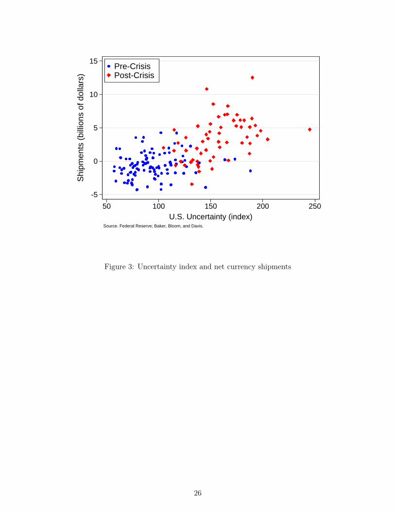
increasing to about 40 percent. In particular, our results suggest that periods of highereconomic uncertainty are associated with higher demand for U.S. banknotes abroad.19 Strongcurrency growth during the financial crisis of 2008 and the subsequent European debt crisisin 2011 support these findings; see Figure 1. This finding is not driven by shipments to aparticular country or a region, as Figure 2 demonstrates. The figure shows annual commercialshipments of currency for two periods (2001-August 2008 and September 2008 to 2013) andfor two sets of countries, Russia and Argentina (the red bars) and all other countries (the graybars). In the most recent period, shipments to Russia and Argentina were higher, but, moreremarkably, shipments to all other countries swung from being negative, on net, to beingstrongly positive and significantly larger than the shipments to Argentina and Russia. Thisfinding is also not driven by an episodic relationship between net shipments and economicuncertainty, as indicated by Figure 3, which shows a scatter plot of the uncertainty indexand net currency shipments, with observations from the pre-crisis and crisis periods clearlymarked. As for the economic significance of the results, note that for the sample period, theuncertainty indexes have a mean of about 100 and standard deviation of about 40. Thus, aone standard deviation move in one index alone is associated with an increase in shipmentsof about $1.2 billion; a simultaneous increase in both indexes is associated with an increaseof about $2.4 billion in monthly shipments.

The last financial crisis provided evidence of stronger co-movements among financialmarkets in advanced economies. For example, episodes centered in the United States wereimmediately discounted in European asset prices, and vice versa.

To allow for these correlations and to further sharpen the focus on economic uncertaintyand financial stress as determinants of U.S. dollar flows, we use principal component analy-sis.20 We extract factors from standardized versions of four inputs: month-average values ofthe VIX and VSTOXX indexes, and the monthly U.S. and European economic policy uncer-tainty indexes.21 These series were chosen as proxy measures of market stress and economicpolicy uncertainty in the United States and advanced Europe. The first principal component(PC), market stress and policy uncertainty, replicates the shared variance of the four inputs,

19The results are robust to the exclusion of U.S. dollar flows to Argentina and Russia from total netshipments as well as to the exclusion of observations for September and October of 2008.

20The factor loadings are elements of eigenvectors obtained from the covariance matrix of the input series.A positive (negative) factor loading for input series i with respect to principal component j indicates positive(negative) correlation between that input series and principal component.

21The VSTOXX index, like the VIX, is not very correlated with shipments on its own, but we include ithere in order to capture European equity volatility.

11

which represents approximately 70 percent of total variance across the four standardizedseries. The second component (policy uncertainty vs. market stress) tracks differences be-tween co-movements of the economic policy uncertainty indices and co-movements of the twomarket stress proxies, and thus can be used to distinguish between the effects on currencydemand of changes in economic policy uncertainty relative to market stress. Analogously,the third PC (U.S. factors vs. European factors) can be used to distinguish between theeffect of changes in U.S. factors relative to changes in European factors.22 Table 3 lists thefactor loadings for the three principal components, the signs and magnitudes of which indi-cate the nature of the correlations between the factors and the four series from which theywere extracted.

As shown in Column 3 of Table 2, the three principal components prove to be helpfulin explaining currency flows. The positive and statistically significant estimate of the firstPC suggests that higher economic and market-related uncertainty in the United States andEurope is related to stronger currency flows. The second PC points to a greater sensitivityof international currency flows to changes in economic policy uncertainty factors relative tochanges in market stress in the United States and Europe. Similarly, estimates for the thirdPC indicate that changes in U.S. economic uncertainty and market stress will have a greaterimpact on international demand for U.S. currency than changes in European uncertaintyfactors. That is, currency flows appear to be more sensitive to U.S. events than to Europeandevelopments. The principal components are constructed to have mean zero and standarddeviation one, so a one standard deviation increase in each principal component is associatedwith an increase of about $1 billion in monthly shipments.

Building on these results, in Column 4 of Table 2 we expand our set of covariates andinclude a group of widely used global macro factors that have been identified in the literatureas potential drivers of demand for U.S. banknotes. Specifically, we evaluate the performanceof global GDP growth, global inflation, the broad U.S. dollar index, oil prices, and goldprices. Whereas estimates for the principal components remain positive and statisticallysignificant, we find no explanatory power of the set of global macroeconomic indicators.These growth rates are expressed in annual percentages (for example, 5 percent annual GDPgrowth would have a value of five).23 Thus, for example, a one percentage point drop inglobal GDP growth is associated with an increase in monthly shipments of $110 million.

As noted previously, and as illustrated in Figures 1 and 2, we conjecture that the factorsdriving international demand for U.S. currency might have changed in 2008. As Baker,Bloom, and Davis (2015) point out, policy uncertainty, as measured by their index, areat extremely elevated levels compared with recent history. Since 2008, economic policyuncertainty has averaged about twice the level of the previous two decades. Based on these

22Appendix B provides an explanation of these factors.23Adding lags did not produce markedly different results.

12

simple observations about aggregate shipment patterns beginning in late 2008, we furtherinvestigate the role of global uncertainty and macro factors by evaluating their explanatorypower in the pre-crisis and crisis periods. To preview the results, we find strong evidencethat suggests that global factors have become important drivers of international currencyflows since the most recent financial crisis.

In Table 4, we begin with the same regression as in the last column of Table 2. InColumn 2, we split the sample into two periods: the “pre-crisis” period (January 2000 toAugust 2008) and the “crisis” period (September 2008 to the end of the sample period).24

The market stress and policy uncertainty PC, our proxy for global economic and marketuncertainty, proves to be economically and statistically significant throughout the differentregression specifications during the crisis period starting in the fourth quarter of 2008. Thesecond PC points in the same direction, with coefficients being positive and statisticallysignificant during the crisis period. Furthermore, whereas the full sample results provide noevidence of the value of global macroeconomic factors as predictors of currency demand, theresults in the third column show that global macro variables such as the broad U.S. dollarindex, oil prices, and global inflation are statistically and economically significant during thecrisis period. Conversely, global GDP growth appears to be a helpful predictor of currencyflows during the pre-crisis period. The negative coefficient indicates that periods of globaleconomic growth are associated with a decrease in total net shipments of U.S. currency notes.

Overall, our aggregate regression analysis provides novel insights into the determinants ofU.S. currency flows. In particular, our results suggest that, over recent years, global uncer-tainty and global macroeconomic factors have become increasingly important determinantsof international demand for U.S. currency.25 To clarify the strength of the uncertainty results,particularly in the crisis period, we consider Baker, Bloom, and Davis (2015)’s measures ofeconomic policy uncertainty, sourced from U.S. and European newspapers. By construction,these measures reflect both domestic and international events that have bearing on economicuncertainty. Moreover, U.S. financial and economic developments tend to have internationalspillovers.

Panel regressions

In this section, we build on our aggregate regression analysis and examine the relation-ship between currency flows and local and global factors using data at the country level.26

24While in some cases it might be necessary to use statistical tests to identify the break between twoperiods, in this case the turning point is clear. It is fairly easily discerned in Figure 1, and it is quite obviousin Figure A1 in Appendix C, where the sharp turn in the red line, for the year 2008, marks the shift.

25The results are robust to the exclusion of U.S. dollar flows to Argentina and Russia from total netshipments as well as to the exclusion of observations for September and October of 2008; these results areavailable on request.

26The data set does not cover U.S. banknote flows between other countries, which may be substantial insome cases—for example, in areas where large volumes of cross-border trade are conducted in cash. The

13

Using a panel data approach, we can examine the effects of country-specific characteristicsand developments on demand for U.S. dollars. As noted earlier, the shipments data set con-tains data for nearly every country in the world. However, as a practical matter, we focus ona subset of about sixty countries for which shipments over time have been non-negligible. Ofthat set of countries, we were able to obtain quarterly or monthly data on income growth,inflation, exchange rates, and equity market volatility for over 40 countries, which are thesubject of our analysis.

Our sample consists of nearly 7,000 country-month observations from January 2000to June 2013 for a group of 42 countries—19 advanced economies, 17 emerging marketeconomies, and 6 currency hubs. In addition to the variables introduced in the aggregate re-gressions, we include country-specific factors that the literature suggests may explain capitalflows: financial market risk; local inflation; foreign exchange reserve growth; and a mea-sure of cumulative net flows, which is defined as cumulative shipments until 2000 scaled byPPP-adjusted GDP in 1999. Our financial market risk factor is a measure of realized equitymarket volatility and is constructed as the monthly variance of the daily growth rates of thelocal equity index. Intuitively, we would expect that higher uncertainty in local financialmarkets will be associated with higher demand for U.S. currency. We include local inflationas a regressor because inflationary episodes have often been associated with increased dollarusage. Also, we consider local foreign exchange reserve growth rates and past cumulative netshipments, which can be interpreted as a measure of the country’s historical experience withU.S. dollar flows. Initially, we also included variables that are often cited as determinants ofmoney demand, such as interest rates and industrial production (a proxy for income), butthese variables had no statistically significant effect and were therefore dropped. Finally, inorder to make the units comparable across countries, we define our dependent variable asthe ratio of net shipments to GDP. More precisely, we annualized monthly net shipmentsand scaled them by annual GDP in U.S. dollars, then expressed the ratio in basis points.

We explore three approaches to estimating a panel model: the random-effects estimator,the fixed-effects estimator, and Hausman and Taylor (1981)’s estimator. The difference be-tween the random-effects model and the fixed-effects model is based on assumptions aboutthe correlation between the individual-specific effects and the set of regressors. In addi-tion, in cases where it is more reasonable to assume that the individual effects are relatedto the regressors, estimation of time-invariant explanatory variables is not possible. Toaddress these issues, Hausman and Taylor (1981) introduced a model where some of theexplanatory variables—observed, time-invariant covariates—are related to the unobserved,individual-specific effects, while others are not. The Hausman-Taylor estimator is consistent

absence of such data does not affect aggregate measurements of commercial bank currency shipment flowsinto and out of the United States. Moreover, worn U.S. banknotes eventually get shipped to the UnitedStates to be replaced, and, hence, will show up in the country-level data.

14

and efficient, does not require any external instruments, and, in contrast to the fixed-effectsestimator, allows estimating coefficients for time-invariant variables.

Based on specification testing (not shown), we settle on a Hausman and Taylor (1981)estimator. Formally, our set up can be summarized as follows:

yi,t = Xi,tβ + Ziη + αi + εi,t, (2)

where i indexes countries, t indexes time, and yi,t is the ratio of net shipments to GDP; Xi,t

is the set of country-specific and global predictors; Zi is the individual past (time-invariant)cumulative shipments; αi is the country fixed effect with mean zero and variance σ2

α; andthe term εi,t stands for i.i.d. errors. Further, Xi,t comprises the set of exogenous covariates,including the principal components uncertainty factors introduced in Table 3, and the set ofcountry-specific covariates, including foreign exchange reserve growth. Zi and the latter setare the endogenous variables in the system due to their correlation with αi.27

Based on the results of the aggregate regressions, we move directly to a specification withseparate coefficients for the pre-crisis and crisis periods, as defined earlier.

Results for countries grouped by the level of economic development

In addition to our observations about the break in the time series in September 2008,country-level shipment patterns and the knowledge gathered through the ICAP suggest thatthe relationship between currency flows and global and local variables might be differentfor different countries. We identify several groups of countries based on the level of theireconomic development (emerging market economies (EMEs) and advanced economies (AEs))and their function in the distribution of U.S. banknotes (currency hubs (hubs) and all othercountries (“AllxHubs”). Table 5 lists of the countries in each group.

Table 6 shows descriptive statistics of the scaled net shipments to countries groupedby the level of economic development and function in the distribution of U.S. currency. Itis immediately clear that net shipments to hubs are very different from those to all othercountries. They are negative, large in absolute magnitude, and very volatile. While averageflows to emerging market economies and advanced economies are comparable in size, theyare an order of magnitude more volatile. As for the economic significance of net shipments,we provide an example for Argentina—a country that discloses such shipments, hence thesedata are not subject to confidentiality. Net shipments to Argentina averaged about $500million a month over the sample period. Hence, the annualized average shipments of $6billion represents about 2 percent of the country’s annual GDP, a substantial percentage.

27We opted not to include country-specific characteristics, such as levels of financial development or mea-sures of capital controls as constructed in Chinn and Ito (2006), because they vary very little over our sampleperiod and cannot be clearly distinguished from country fixed effects. We note, though, that past cumulativeshipments may be correlated with some of the country-specific characteristics.

15

Regression results by country group are reported in Table 8, with the results for the fullpanel in Column 1.28 The results for the full panel are broadly similar to the aggregate resultsand in line with our expectations, though there are a few exceptions. As in the aggregateregressions, the measures of global uncertainty are positive and statistically significant forthe first two factors during the crisis period, but are statistically insignificant in the pre-crisisperiod. Country-specific estimates for equity market volatility and inflation are positive andstatistically significant for both periods in the full panel.29 However, while the economicsignificance of local financial market volatility appears stronger in the pre-crisis period,domestic inflation plays a larger role in explaining currency flows in the crisis period. Also,cumulative net shipments, our measure of the country’s historical experience with U.S. dollarflows, is positive and statistically significant. Conversely, we find a negative relationshipbetween foreign exchange reserve growth and currency flows.30

The full panel regression combines countries whose experiences with, and uses of, dollarsare quite disparate. As a result, some of the effects of the predictors on currency flows mightgo in opposite directions or even cancel out when pooling the data. To account for this issueand to gain a better understanding of currency flows dynamics in the next regressions, weexamine these relationships for groups of countries that we expect to be more homogenous,either because of their level of development, their role in the distribution system for dollars,or their position as a net importer or exporter of dollars. Column 2 in Table 8 reportsregressions estimated just for emerging market economies. For these countries, the isolatedglobal uncertainty component is statistically significant, and only in the crisis period. Asfor the local predictors, the coefficients for equity-market volatility and inflation are positiveand statistically significant in both periods, while foreign exchange reserve growth is negativeand statistically significant during the pre-crisis period. Notably, the R2 for this group ofcountries is considerably higher, at nearly 60 percent. Our robustness checks (not shown)suggest that these results are driven by shipments to either Eastern Europe or the formerSoviet Union.

Column 3 of Table 8 reports results for advanced economies. In general, dollar usage inthese countries appears to be minimal and limited to tourism. Not surprisingly, coefficientestimates are generally small in magnitude; relatively few are statistically significant; andthe R2 is quite low, at about 25 percent. Column 4 reports results for a group of countries

28We exclude hubs—for example, Austria and the United Kingdom—from the full panel regressions, astheir demand for U.S. currency can be expected to be uncorrelated with the country’s fundamentals. Whilethey are home to large banknote retailers and major international airports, there is little evidence of domesticuse of dollars. The full panel results are robust to the inclusion of hub countries in the panel.

29The differences between the coefficient estimates in the two periods are statistically significant at the 10percent level.

30Exclusion of this variable does not affect our results. Recall that elevated demand for U.S. dollars isa form of capital flight (by residents of these countries), and it appears to result in loss of official foreignreserves.

16

that appear to function largely as distribution centers for currency. For these countries,there is little evidence of domestic use of dollars; at the same time, they are home to largebanknote retailers and major international airports. Information gathered during the ICAPproject indicated that most of the dollars shipped to or from these countries had come fromthird countries. Coefficients on local inflation and the second principal component factorthat isolates global uncertainty from market stress are significant for these countries.

Results for countries grouped by the patterns of currency flows

We identify several groups of countries based on the patterns of currency flows: countrieswith large flows of U.S. banknotes in either direction (Big), countries with large positiveinflows (BigNetPos), countries with large negative outflows (BigNetNeg), countries withpersistent inflows (NetPos), and countries with persistent outflows (NetNeg). Table 5 listsof the countries in each group.

Table 7 shows descriptive statistics for net shipments to countries grouped by the patternsof currency flows. Net shipments for “Big” countries average to about zero because roughlyhalf of these countries receive large shipments of U.S. banknotes, while the other half shipU.S. banknotes to the United States in similar quantities. Countries that tend to have largeinflows of U.S. currency received, on average, roughly similar amounts in the pre- and post-crisis periods. However, countries that tend to have large outflows of U.S. currency shippedto the United States, on average, slightly lower amounts in the post-crisis period.

Results for panel regressions based on these criteria are shown in Table 9. Column 1 showsthe results for the full sample, as in Table 8. The following columns group the countries intothose that have shown large shipments relative to GDP and overall (“Big”), those whichshipments are positive overall (“NetPos”), those which shipments are both large and positive(“BigPos”), and the same for negative net shipments (“NetNeg” and “BigNeg”). In theseresults, local equity market volatility is consistently positive and statistically significant inthe pre-crisis period but not in the crisis period. Local inflation is nearly always statisticallysignificant and positive in both periods. Measures of uncertainty are more strongly andconsistently positive and statistically significant during the crisis period.

Economic significance

Figure 4 summarizes the contributions to net currency shipments of local variables (thered bars) and global variables (the blue bars) over the pre- and post-crisis periods based onthe regression results Tables 8 and 9. (Recall that we annualized monthly net shipmentsscaled by annual GDP in U.S. dollars, and expressed the ratio in basis points.) As panel1 shows for all countries excluding hubs (“AllxHubs”), the contributions of global factorswere negative prior to the crisis (about -30 basis points) but slightly positive during the

17

post-crisis (a few basis points); local variables appeared to have about the same contribu-tion in both periods (about 40 basis points). Across countries grouped by their economicdevelopment or function in currency distribution, the contribution of global factors changedsign and increased in magnitude over time, especially in emerging market economies (panel2) and currency hubs that tend to supply U.S. dollars to emerging market economies (panel4). While we observe a similar pattern for advanced economies, we should note that themagnitudes of the contribution of global factors are small. This finding does not indicatethat U.S. dollars function as a safe asset in these countries, but rather suggests that thesecountries may have functioned like currency hubs. Across countries grouped by the patternsof currency flows, for countries where dollar usage is substantial—for example, those in the“BigPos” group, which includes Russia, Ukraine, and Kazakhstan—we observe patterns andmagnitudes similar to those for emerging market economies.

Low- and high-frequency results by country groups

As indicated earlier, economic or political crises in specific regions or countries coincidedwith episodic increases in net currency shipments to destinations such as Argentina and theformer Soviet Union, so it might be reasonable to suppose that the impact of global riskand economic uncertainty is also episodic. In the spirit of Forbes and Warnock (2012), weevaluate the ability of both local and global factors to explain both low- and high-frequencycomponents of currency flows. After all, banknote flows are the physical component offinancial capital flows. Since the demand for U.S. currency abroad stems from its use as asafe asset, net currency shipments may exhibit behavior similar to international capital flowsduring periods of increased global risk. As discussed earlier, elevated precautionary demandfor U.S. banknotes is a form of capital flight out of the affected country.

We test this possibility by isolating low-frequency and high-frequency components of theshipments data using the band pass filter developed by Christiano and Fitzgerald (2003).31

We estimate high-frequency components corresponding to periods of up to 12 months andlow-frequency components corresponding to periods of no less than 12 months.32 Seasonalfluctuations were therefore included in the high-frequency component along with transitoryfluctuations. An examination of the data indicates that seasonal fluctuations are negligiblefor most cross-sections, and the high-frequency components therefore primarily reflect tran-sitory fluctuations that would include episodic increases and decreases lasting up to a year.33

31The band pass filter is “asymmetric,” meaning that the weights applied to observations at times t + qand t− q in the estimation of the filtered component at time t are not necessarily the same. We chose thisfilter because it allowed us to estimate frequency components for our entire data set, whereas the use of asymmetric filter would have resulted in a meaningful loss of data through truncation.

32In Forbes and Warnock (2012), surges of various types last, on average, between three and four quarters.This difference in choice of frequency threshold and the differences in frequency decomposition methodsmake our and their results not directly comparable.

33The use of asymmetric weights produces phase shifts in the filtered components that can cause fluctua-

18

The low-frequency components reflect more persistent phenomena.As shown in Tables 10 and 11, the results of regressions using low-frequency components

were broadly similar to those estimated on unfiltered net shipments. The magnitudes ofthe coefficient estimates for the two global risk principal components were typically smallerwhen low-frequency components were used, likely because of the reduced variances of thedependent variables.34 Although smaller in magnitude, most of the coefficients obtainedfrom the low-frequency regressions had the same signs as those obtained from regressionsusing the unfiltered data, and most of the coefficients that were statistically significant whenthe unfiltered data were used were also significant when the low-frequency components wereused. These results suggest that the relationship between global uncertainty and currencyflows is persistent rather than episodic. It may be that U.S. dollars, as a safe asset, providehedging benefits on average rather just in times of stress. It may also be that times ofstress in emerging market economies are long-lasting, leading to persistent demand for U.S.dollars. Indeed, in contrast to VIX, news-based uncertainty measures are very persistent,likely reflecting long crisis spells.

We omit the results for high-frequency components because of the general absence of theirstatistical significance. Foreign exchange reserves are the only variable that appears to haverobust negative correlation with the flows for emerging market economies and countries withlarge inflows of U.S. banknotes, but their explanatory power is extremely low. In addition,the correlation may be, to some extent, mechanical.

5 Implications of currency demand from abroad for the Federal

Reserve’s operations

Understanding the demand for currency has consistently played an important role inFederal Reserve operations, both in the implementation of monetary policy and in the lo-gistical planning needed to supply banknotes of high quality in adequate quantities.35 Fromthe 1990s until late 2008, the Federal Reserve targeted the federal funds rate by adjustingthe supply of reserve balances, in part to offset changes in demand for currency (which add

tions that are unsynchronized with fluctuations in the raw data. We looked for evidence of significant phaseshifts by calculating cross correlations between the raw data and the low-frequency components at leads andlags of up to 36 months. If filtering had resulted in significant shifts, the misalignment of fluctuations wouldhave resulted in higher correlation of the raw data to leads or lags of the low-frequency components thanto the contemporaneous components. For each cross-section in our data set, the raw data were more highlycorrelated to the contemporaneous low-frequency components than to components at any lead or lag, whichsuggests that phase shifts were negligible.

34By removing the high-frequency components, we left less variance to be explained by the regressors.For most of the countries in our sample, removal of the high-frequency components reduced variance by 25to 40 percent. R2 values for the low-frequency regressions were higher despite the smaller magnitudes ofthe regression coefficients, suggesting that the primary reason for the smaller coefficient estimates was thereduced variances of the dependent variables rather than a deterioration in the quality of the goodness of fit.

35For more details, see Board of Governors of the Federal Reserve System (2006).

19

or drain reserve balances). At that time, currency in circulation was the primary liabilityon the Federal Reserve’s balance sheet (shown in green in Figure 5) and changes in currencydemand were a major consideration in the conduct of daily open market operations as wellas in longer-range planning related to the Federal Reserve’s System Open Market Accountportfolio.36

After late 2008, deposits of depository institutions at the Federal Reserve (that is, re-serve balances in the banking system), shown in gray, increased significantly, and they nowgreatly exceed currency as the largest liability on the Federal Reserve’s balance sheet. Pro-jected currency growth nonetheless remains an important input into planning for the FederalReserve’s exit from its current asset purchase programs and, ultimately, balance-sheet nor-malization. In particular, in the case of normalization, the higher the currency growth, themore reserve balances are drained by this autonomous factor. This increase in currency incirculation reduces the quantity of U.S. Treasury securities that the Federal Reserve needsto sell to reduce the size of its balance sheet. In addition, in the process, the Federal Reservewill spend less on remuneration of reserve balances and, hence, will remit more to the U.S.Treasury. We work out such an example in Appendix C.

6 Conclusions

Across a few dozen countries and nearly a decade and a half, we find that both globaland local factors explain shipments of U.S. dollars abroad. In the aggregate, where onlyglobal factors appear to be relevant, we find that net shipments of dollars from the UnitedStates to other countries are very strongly correlated with measures of financial and eco-nomic uncertainty in the period since 2008 and considerably less so in earlier years. Thesecorrelations reflect a persistent, rather than episodic, relationship between currency flowsand their determinants, such as uncertainty. Two interpretations appear to be consistentwith this finding. First, U.S. dollars, as a safe asset, may provide hedging benefits on aver-age rather just in times of stress. Second, times of stress in emerging market economies maybe long-lasting, leading to persistent demand for U.S. dollars. Indeed, in contrast to VIX,news-based uncertainty measures are very persistent, likely reflecting long crisis spells.

For various country groupings, we evaluate the ability of both local and global factorsto explain currency flows. We show that, since the global financial crisis, global economic

36On the operational side, the Federal Reserve is responsible for overseeing or implementing a wide arrayof tasks related to the production, distribution, use, and destruction of Federal Reserve notes. The FederalReserve works with the Treasury’s Bureau of Engraving and Printing to determine banknote design andproduction schedules. The Federal Reserve is then responsible for the storage, distribution, processing, anddestruction of currency at its offices. The Federal Reserve also determines policies for banknote handling bycommercial banks and, in cooperation with the Treasury, provides public education as necessary. Finally,the Federal Reserve works with the Treasury and the United States Secret Service to monitor and reducecounterfeiting.

20

uncertainty has had an increasingly important role in explaining dollar flows, particularly toemerging market economies. The results also suggest a greater sensitivity of demand fromabroad for U.S. banknotes to changes in economic uncertainty relative to changes in financialmarket stress. While currency flows to currency hubs (advanced countries that do not useU.S. banknotes but supply them to other countries and regions) also tend to respond toglobal economic uncertainty, those to advanced economies do not. These findings supportthe narrative that U.S. banknotes are used as a safe asset in emerging market economies. Inaddition, we show that local factors, such as inflation, also play a role in explaining currencyflows. Similarly, when we group countries based on their flow patterns rather than theireconomic development, country-specific characteristics still predict dollar flows. In contrastto money demand theory, demand for U.S. currency appears to be interest rate insensitive.

In the spirit of the capital flows literature, we examine the ability of local and globalfactors to explain both low- and high-frequency components of currency flows. We find thatthe relationship between global uncertainty and U.S. dollar flows is persistent rather thanepisodic.

Our analysis has important implications for policy makers. From the perspective offoreign central banks, particularly those in emerging market economies, understanding andquantifying factors affecting demand for U.S. banknotes as a safe asset is crucial for theiroperations, including determining a desired size of foreign exchange reserves. In this context,one novel findings is the increased importance of global factors as determinants of currencyflows for a given country. From the domestic perspective, understanding the factors drivinginternational dollar flows—a major component of currency growth—is important for a widerange of Federal Reserve operational considerations and for the normalization of monetarypolicy.

Going forward, we envisage studying the implications of demand for U.S. banknotes fromabroad on the Federal Reserve’s operations and, hence, U.S. financial market functioning inmore detail. In addition, for emerging market economies, we intend to explore the con-struction of risk or uncertainty indexes using our cross-border currency flow data and othercountry- or region-specific variables.37

References

Baker, S. R., N. Bloom, and S. J. Davis (2015): “Measuring economic policy uncer-tainty,” mimeo.

37We can use the data as a measure of demand that relates to risk factors. For example, we can run apush-pull model of broader capital flows (other than currency flows), with currency flows as an explanatoryfactor that captures local risk. This approach may capture local factors that are, otherwise, very hard toproxy.

21

Bartzsch, N., G. Rosl, and F. Seitz (2013): “Currency movements within and outsidea currency union: The case of Germany and the euro area,” The Quarterly Review ofEconomics and Finance, 53(4), 393–401.

Blanchard, O., M. Das, and H. Faruqee (2010): “The initial impact of the crisis onemerging market countries,” Brookings Papers on Economic Activity, Spring, 263–307.

Board of Governors of the Federal Reserve System (2006): Purposes and func-tions. Washington, DC.

Calvo, G. A., L. Leiderman, and C. M. Reinhart (1993): “Capital inflows and realexchange rate appreciation in Latin America: The role of external factors,” InternationalMonetary Fund Staff Papers, 40(1), 108–151.

Chinn, M. D., and H. Ito (2006): “What matters for financial development? Capitalcontrols, institutions, and interactions,” Journal of Development Economics, 81(1), 163–192.

Christiano, L. J., and T. J. Fitzgerald (2003): “The band pass filter,” InternationalEconomic Review, 44(2), 435–465.

Chuhan, P., S. Claessens, and N. Mamingi (1998): “Equity and bond flows to LatinAmerica and Asia: The role of global and country factors,” Journal of Development Eco-nomics, 55(2), 439–463.

Claessens, S., and K. Forbes (2004): “International financial contagion: The theory,evidence and policy implications,” mimeo.

Doyle, B. (2000): “’Here, dollars, dollars...’—estimating currency demand and worldwidecurrency substitution,” International Finance Discussion Paper, 657.

Fernandez-Arias, E. (1996): “The new wave of private capital inflows: Push or pull?,”Journal of Development Economics, 48(2), 389–418.

Fischer, B., P. Kohler, and F. Seitz (2004): “The Demand for euro area currencies:Past, present, and future,” European Central Bank Working Paper, 330.

Forbes, K. (2004): “The Asian flu and Russian virus: The international transmission ofcrises in firm-level data,” Journal of International Economics, 63(1), 59–92.

Forbes, K. J., and F. E. Warnock (2012): “Capital flow waves: Surges, stops, flight,and retrenchment,” Journal of International Economics, 88(2), 235–251.

Fratzscher, M. (2012): “Capital flows, push versus pull factors and the global financialcrisis,” Journal of International Economics, 88(2), 341 – 356.

Ghosh, A. R., M. S. Qureshi, J. I. Kim, and J. Zalduendo (2014): “Surges,” Journalof International Economics, 92(2), 266 – 285.

Gourio, F., M. Siemer, and A. Verdelhan (2014): “Uncertainty and internationalcapital flows,” mimeo.

22

Greenlaw, D., J. D. Hamilton, P. Hooper, and F. S. Mishkin (2013): “Crunch time:Fiscal crises and the role of monetary policy,” NBER Working Paper, No. 19297.

Griffin, J., F. Nardari, and R. Stulz (2004): “Daily cross-border flows: Pushed orpulled?,” Review of Economics and Statistics, 86(3), 641–657.

Hausman, J. A., and W. E. Taylor (1981): “Panel data and unobservable individualeffects,” Econometrica, 49(6), 1377–1398.

Hellerstein, R., and W. Ryan (2011): “Cash dollars abroad,” Federal Reserve Bank ofNew York Reports, (400).

Judson, R. A. (2012): “Crisis and calm: Demand for U.S. currency at home and abroadfrom the fall of the Berlin Wall to 2011,” Federal Reserve International Finance DiscussionPaper, 1058.

Judson, R. A., and R. D. Porter (1996): “The location of U.S. currency: How much isabroad?,” Federal Reserve Bulletin, 82, 883–903.

Kamin, S. B., and N. R. Ericsson (2003): “Dollarization in post-hyperinflationary Ar-gentina,” Journal of International Money and Finance, 22(2), 185 – 211.

Stix, H. (2010): “Euroization: What factors drive its persistence? Household data evidencefor Croatia, Slovenia, and Slovakia,” Applied Economics, 32(21), 2689–2704.

U.S. Census Bureau (2012): Statistical Abstract of the United States. Washington, DC.

U.S. Department of the Treasury (2006): The use and counterfeiting of U.S. currencyabroad, part III. Washington, DC.

23

-5

0

5

10

15

Bill

ions

of d

olla

rs

Jan

2000

Jan

2001

Jan

2002

Jan

2003

Jan

2004

Jan

2005

Jan

2006

Jan

2007

Jan

2008

Jan

2009

Jan

2010

Jan

2011

Jan

2012

Jan

2013

Jan

2014

Figure 1: Monthly net shipments of U.S. dollars, in aggregate

24

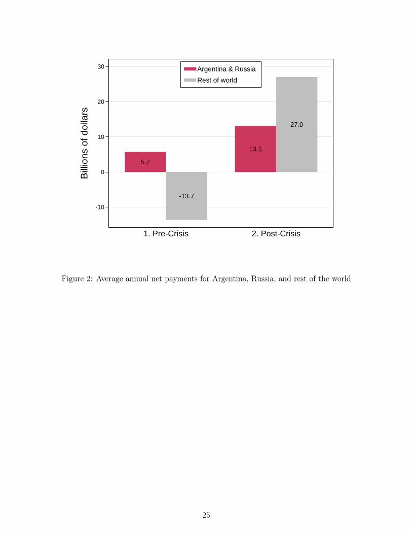
5.7

-13.7

13.1

27.0

-10

0

10

20

30

Bill

ions

of d

olla

rs

1. Pre-Crisis 2. Post-Crisis

Argentina & Russia

Rest of world

Figure 2: Average annual net payments for Argentina, Russia, and rest of the world

25

-5

0

5

10

15

Shi

pmen

ts (

billi

ons

of d

olla

rs)

50 100 150 200 250U.S. Uncertainty (index)

Pre-CrisisPost-Crisis

Source. Federal Reserve; Baker, Bloom, and Davis.

Figure 3: Uncertainty index and net currency shipments

26

-40

-20

0

20

40

-50

0

50

100

-10

-5

0

5

0

100

200

300

400

-20

0

20

40

60

-20

0

20

40

60

80

-20

-10

0

10

20

30

-40

-20

0

20

40

-20

0

20

40

60

Pre Post Pre Post Pre Post Pre Post Pre Post

Pre Post Pre Post Pre Post Pre Post

01_AllxHubs 02_EMEs 03_AEs 04_Hubs 05_Big

06_BigPos 07_BigNeg 08_NetPos 09_NetNeg

Local Global

Figure 4: Factor contributions to net currency shipments for all countries, including hubs(basis points of GDP in U.S. dollars)

27

Assets

Liabilities and Capital

Loans andliquidity

programs

Agency debt and mortgage-backedsecurities

Repurchase agreements and all other assets

¯

Treasuries, >5 years

Treasuries, 1-5 years

Treasuries, <1 year

Federal Reserve notes in circulation

­Reverse RPs, capital,

and all other liabilities

U.S. Treasury accounts

Deposits of depository institutions and other deposits

0

1,000

2,000

3,000

4,000

5,000

5,000

4,000

3,000

2,000

1,000

Bill

ions

of d

olla

rs

Jan 3, 2007 Jan 3, 2008 Jan 2, 2009 Jan 2, 2010 Jan 2, 2011 Jan 2, 2012 Jan 1, 2013 Jan 1, 2014

Source: H.4.1 Statistical Release (http://www.federalreserve.gov/releases/h41/).

Figure 5: Federal Reserve assets and liabilities, 2007–2014

Table 1: Monthly net shipments in aggregate, millions of U.S. dollars

Number of Net shipmentsobservations Mean Stand.dev. Median 5th pct 95th pct

Full sample 162 777 3,079 4 -3,463 6,398Pre-crisis 104 -666 1,869 -810 -3,814 2,658Crisis 58 3,364 3,140 3,322 -1,165 8,557

28

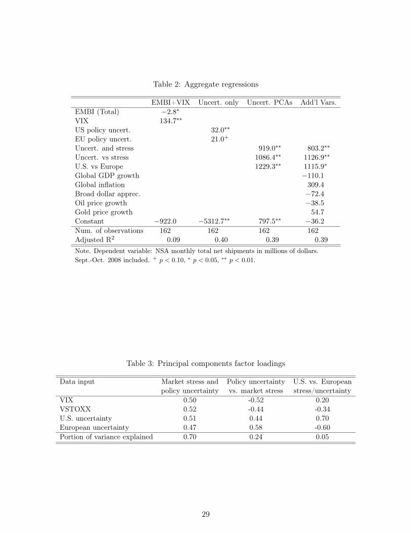
Table 2: Aggregate regressions

EMBI+VIX Uncert. only Uncert. PCAs Add’l Vars.EMBI (Total) −2.8∗

VIX 134.7∗∗

US policy uncert. 32.0∗∗

EU policy uncert. 21.0+

Uncert. and stress 919.0∗∗ 803.2∗∗

Uncert. vs stress 1086.4∗∗ 1126.9∗∗

U.S. vs Europe 1229.3∗∗ 1115.9∗

Global GDP growth −110.1Global inflation 309.4Broad dollar apprec. −72.4Oil price growth −38.5Gold price growth 54.7Constant −922.0 −5312.7∗∗ 797.5∗∗ −36.2

Num. of observations 162 162 162 162Adjusted R2 0.09 0.40 0.39 0.39

Note. Dependent variable: NSA monthly total net shipments in millions of dollars.Sept.-Oct. 2008 included. + p < 0.10, ∗ p < 0.05, ∗∗ p < 0.01.

Table 3: Principal components factor loadings

Data input Market stress and Policy uncertainty U.S. vs. Europeanpolicy uncertainty vs. market stress stress/uncertainty

VIX 0.50 -0.52 0.20VSTOXX 0.52 -0.44 -0.34U.S. uncertainty 0.51 0.44 0.70European uncertainty 0.47 0.58 -0.60Portion of variance explained 0.70 0.24 0.05

29

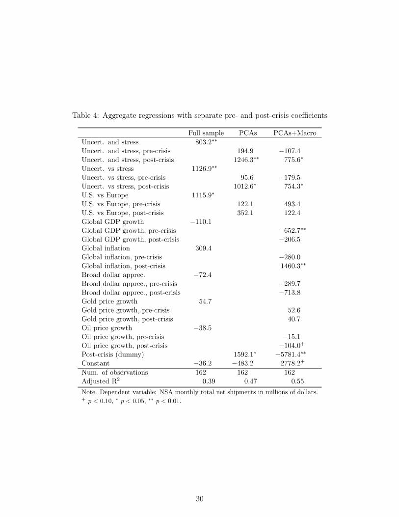
Table 4: Aggregate regressions with separate pre- and post-crisis coefficients

Full sample PCAs PCAs+MacroUncert. and stress 803.2∗∗

Uncert. and stress, pre-crisis 194.9 −107.4Uncert. and stress, post-crisis 1246.3∗∗ 775.6∗

Uncert. vs stress 1126.9∗∗

Uncert. vs stress, pre-crisis 95.6 −179.5Uncert. vs stress, post-crisis 1012.6∗ 754.3∗

U.S. vs Europe 1115.9∗

U.S. vs Europe, pre-crisis 122.1 493.4U.S. vs Europe, post-crisis 352.1 122.4Global GDP growth −110.1Global GDP growth, pre-crisis −652.7∗∗

Global GDP growth, post-crisis −206.5Global inflation 309.4Global inflation, pre-crisis −280.0Global inflation, post-crisis 1460.3∗∗

Broad dollar apprec. −72.4Broad dollar apprec., pre-crisis −289.7Broad dollar apprec., post-crisis −713.8Gold price growth 54.7Gold price growth, pre-crisis 52.6Gold price growth, post-crisis 40.7Oil price growth −38.5Oil price growth, pre-crisis −15.1Oil price growth, post-crisis −104.0+

Post-crisis (dummy) 1592.1∗ −5781.4∗∗

Constant −36.2 −483.2 2778.2+

Num. of observations 162 162 162Adjusted R2 0.39 0.47 0.55

Note. Dependent variable: NSA monthly total net shipments in millions of dollars.+ p < 0.10, ∗ p < 0.05, ∗∗ p < 0.01.

30

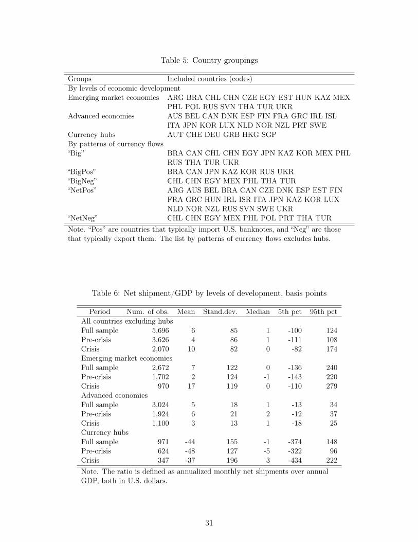
Table 5: Country groupings

Groups Included countries (codes)By levels of economic developmentEmerging market economies ARG BRA CHL CHN CZE EGY EST HUN KAZ MEX

PHL POL RUS SVN THA TUR UKRAdvanced economies AUS BEL CAN DNK ESP FIN FRA GRC IRL ISL

ITA JPN KOR LUX NLD NOR NZL PRT SWECurrency hubs AUT CHE DEU GRB HKG SGPBy patterns of currency flows“Big” BRA CAN CHL CHN EGY JPN KAZ KOR MEX PHL

RUS THA TUR UKR“BigPos” BRA CAN JPN KAZ KOR RUS UKR“BigNeg” CHL CHN EGY MEX PHL THA TUR“NetPos” ARG AUS BEL BRA CAN CZE DNK ESP EST FIN

FRA GRC HUN IRL ISR ITA JPN KAZ KOR LUXNLD NOR NZL RUS SVN SWE UKR

“NetNeg” CHL CHN EGY MEX PHL POL PRT THA TURNote. “Pos” are countries that typically import U.S. banknotes, and “Neg” are thosethat typically export them. The list by patterns of currency flows excludes hubs.

Table 6: Net shipment/GDP by levels of development, basis points

Period Num. of obs. Mean Stand.dev. Median 5th pct 95th pctAll countries excluding hubsFull sample 5,696 6 85 1 -100 124Pre-crisis 3,626 4 86 1 -111 108Crisis 2,070 10 82 0 -82 174Emerging market economiesFull sample 2,672 7 122 0 -136 240Pre-crisis 1,702 2 124 -1 -143 220Crisis 970 17 119 0 -110 279Advanced economiesFull sample 3,024 5 18 1 -13 34Pre-crisis 1,924 6 21 2 -12 37Crisis 1,100 3 13 1 -18 25Currency hubsFull sample 971 -44 155 -1 -374 148Pre-crisis 624 -48 127 -5 -322 96Crisis 347 -37 196 3 -434 222Note. The ratio is defined as annualized monthly net shipments over annualGDP, both in U.S. dollars.

31

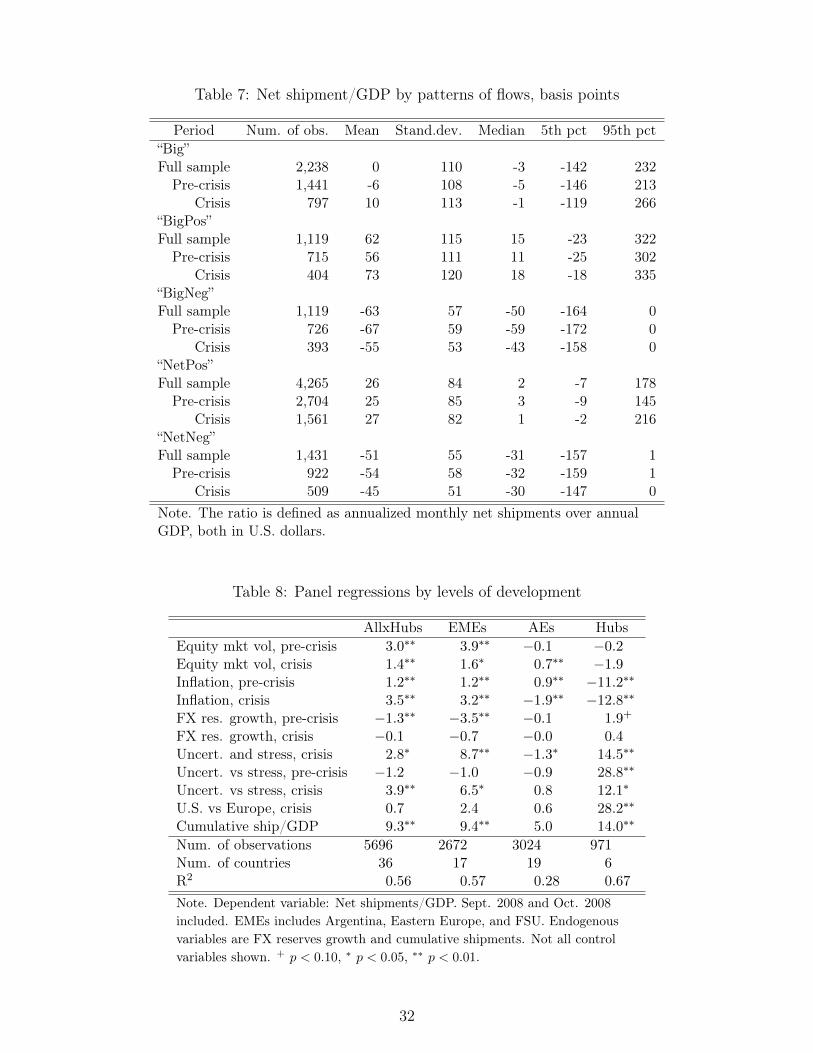
Table 7: Net shipment/GDP by patterns of flows, basis points

Period Num. of obs. Mean Stand.dev. Median 5th pct 95th pct“Big”Full sample 2,238 0 110 -3 -142 232Pre-crisis 1,441 -6 108 -5 -146 213

Crisis 797 10 113 -1 -119 266“BigPos”Full sample 1,119 62 115 15 -23 322Pre-crisis 715 56 111 11 -25 302

Crisis 404 73 120 18 -18 335“BigNeg”Full sample 1,119 -63 57 -50 -164 0Pre-crisis 726 -67 59 -59 -172 0

Crisis 393 -55 53 -43 -158 0“NetPos”Full sample 4,265 26 84 2 -7 178Pre-crisis 2,704 25 85 3 -9 145

Crisis 1,561 27 82 1 -2 216“NetNeg”Full sample 1,431 -51 55 -31 -157 1Pre-crisis 922 -54 58 -32 -159 1

Crisis 509 -45 51 -30 -147 0Note. The ratio is defined as annualized monthly net shipments over annualGDP, both in U.S. dollars.

Table 8: Panel regressions by levels of development

AllxHubs EMEs AEs HubsEquity mkt vol, pre-crisis 3.0∗∗ 3.9∗∗ −0.1 −0.2Equity mkt vol, crisis 1.4∗∗ 1.6∗ 0.7∗∗ −1.9Inflation, pre-crisis 1.2∗∗ 1.2∗∗ 0.9∗∗ −11.2∗∗

Inflation, crisis 3.5∗∗ 3.2∗∗ −1.9∗∗ −12.8∗∗

FX res. growth, pre-crisis −1.3∗∗ −3.5∗∗ −0.1 1.9+

FX res. growth, crisis −0.1 −0.7 −0.0 0.4Uncert. and stress, crisis 2.8∗ 8.7∗∗ −1.3∗ 14.5∗∗

Uncert. vs stress, pre-crisis −1.2 −1.0 −0.9 28.8∗∗

Uncert. vs stress, crisis 3.9∗∗ 6.5∗ 0.8 12.1∗

U.S. vs Europe, crisis 0.7 2.4 0.6 28.2∗∗

Cumulative ship/GDP 9.3∗∗ 9.4∗∗ 5.0 14.0∗∗

Num. of observations 5696 2672 3024 971Num. of countries 36 17 19 6R2 0.56 0.57 0.28 0.67

Note. Dependent variable: Net shipments/GDP. Sept. 2008 and Oct. 2008included. EMEs includes Argentina, Eastern Europe, and FSU. Endogenousvariables are FX reserves growth and cumulative shipments. Not all controlvariables shown. + p < 0.10, ∗ p < 0.05, ∗∗ p < 0.01.

32

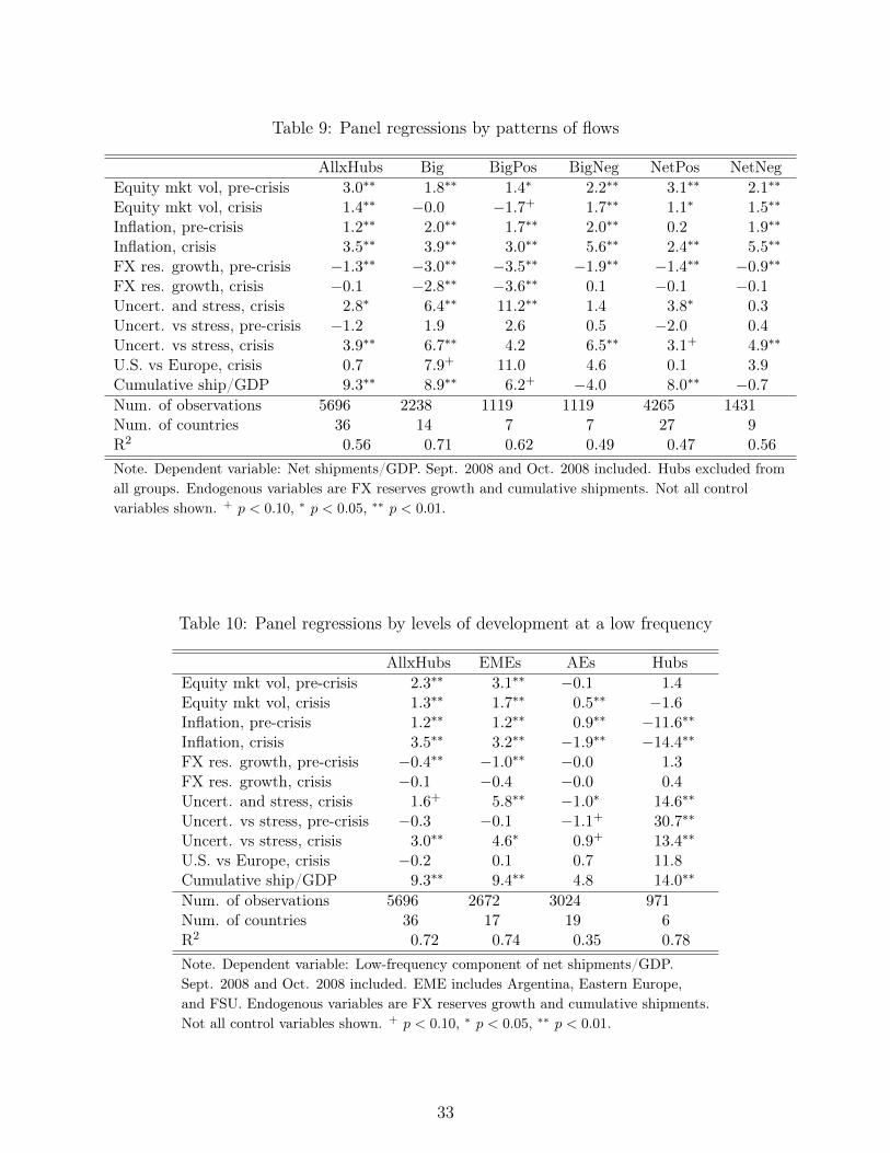
Table 9: Panel regressions by patterns of flows

AllxHubs Big BigPos BigNeg NetPos NetNegEquity mkt vol, pre-crisis 3.0∗∗ 1.8∗∗ 1.4∗ 2.2∗∗ 3.1∗∗ 2.1∗∗

Equity mkt vol, crisis 1.4∗∗ −0.0 −1.7+ 1.7∗∗ 1.1∗ 1.5∗∗

Inflation, pre-crisis 1.2∗∗ 2.0∗∗ 1.7∗∗ 2.0∗∗ 0.2 1.9∗∗

Inflation, crisis 3.5∗∗ 3.9∗∗ 3.0∗∗ 5.6∗∗ 2.4∗∗ 5.5∗∗

FX res. growth, pre-crisis −1.3∗∗ −3.0∗∗ −3.5∗∗ −1.9∗∗ −1.4∗∗ −0.9∗∗

FX res. growth, crisis −0.1 −2.8∗∗ −3.6∗∗ 0.1 −0.1 −0.1Uncert. and stress, crisis 2.8∗ 6.4∗∗ 11.2∗∗ 1.4 3.8∗ 0.3Uncert. vs stress, pre-crisis −1.2 1.9 2.6 0.5 −2.0 0.4Uncert. vs stress, crisis 3.9∗∗ 6.7∗∗ 4.2 6.5∗∗ 3.1+ 4.9∗∗

U.S. vs Europe, crisis 0.7 7.9+ 11.0 4.6 0.1 3.9Cumulative ship/GDP 9.3∗∗ 8.9∗∗ 6.2+ −4.0 8.0∗∗ −0.7

Num. of observations 5696 2238 1119 1119 4265 1431Num. of countries 36 14 7 7 27 9R2 0.56 0.71 0.62 0.49 0.47 0.56

Note. Dependent variable: Net shipments/GDP. Sept. 2008 and Oct. 2008 included. Hubs excluded fromall groups. Endogenous variables are FX reserves growth and cumulative shipments. Not all controlvariables shown. + p < 0.10, ∗ p < 0.05, ∗∗ p < 0.01.

Table 10: Panel regressions by levels of development at a low frequency

AllxHubs EMEs AEs HubsEquity mkt vol, pre-crisis 2.3∗∗ 3.1∗∗ −0.1 1.4Equity mkt vol, crisis 1.3∗∗ 1.7∗∗ 0.5∗∗ −1.6Inflation, pre-crisis 1.2∗∗ 1.2∗∗ 0.9∗∗ −11.6∗∗

Inflation, crisis 3.5∗∗ 3.2∗∗ −1.9∗∗ −14.4∗∗

FX res. growth, pre-crisis −0.4∗∗ −1.0∗∗ −0.0 1.3FX res. growth, crisis −0.1 −0.4 −0.0 0.4Uncert. and stress, crisis 1.6+ 5.8∗∗ −1.0∗ 14.6∗∗

Uncert. vs stress, pre-crisis −0.3 −0.1 −1.1+ 30.7∗∗

Uncert. vs stress, crisis 3.0∗∗ 4.6∗ 0.9+ 13.4∗∗

U.S. vs Europe, crisis −0.2 0.1 0.7 11.8Cumulative ship/GDP 9.3∗∗ 9.4∗∗ 4.8 14.0∗∗

Num. of observations 5696 2672 3024 971Num. of countries 36 17 19 6R2 0.72 0.74 0.35 0.78

Note. Dependent variable: Low-frequency component of net shipments/GDP.Sept. 2008 and Oct. 2008 included. EME includes Argentina, Eastern Europe,and FSU. Endogenous variables are FX reserves growth and cumulative shipments.Not all control variables shown. + p < 0.10, ∗ p < 0.05, ∗∗ p < 0.01.

33

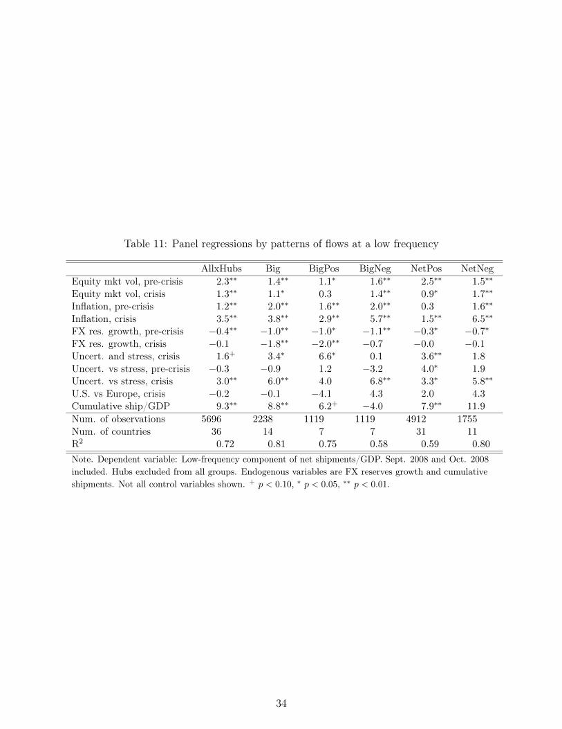
Table 11: Panel regressions by patterns of flows at a low frequency

AllxHubs Big BigPos BigNeg NetPos NetNegEquity mkt vol, pre-crisis 2.3∗∗ 1.4∗∗ 1.1∗ 1.6∗∗ 2.5∗∗ 1.5∗∗

Equity mkt vol, crisis 1.3∗∗ 1.1∗ 0.3 1.4∗∗ 0.9∗ 1.7∗∗

Inflation, pre-crisis 1.2∗∗ 2.0∗∗ 1.6∗∗ 2.0∗∗ 0.3 1.6∗∗

Inflation, crisis 3.5∗∗ 3.8∗∗ 2.9∗∗ 5.7∗∗ 1.5∗∗ 6.5∗∗

FX res. growth, pre-crisis −0.4∗∗ −1.0∗∗ −1.0∗ −1.1∗∗ −0.3∗ −0.7∗

FX res. growth, crisis −0.1 −1.8∗∗ −2.0∗∗ −0.7 −0.0 −0.1Uncert. and stress, crisis 1.6+ 3.4∗ 6.6∗ 0.1 3.6∗∗ 1.8Uncert. vs stress, pre-crisis −0.3 −0.9 1.2 −3.2 4.0∗ 1.9Uncert. vs stress, crisis 3.0∗∗ 6.0∗∗ 4.0 6.8∗∗ 3.3∗ 5.8∗∗

U.S. vs Europe, crisis −0.2 −0.1 −4.1 4.3 2.0 4.3Cumulative ship/GDP 9.3∗∗ 8.8∗∗ 6.2+ −4.0 7.9∗∗ 11.9

Num. of observations 5696 2238 1119 1119 4912 1755Num. of countries 36 14 7 7 31 11R2 0.72 0.81 0.75 0.58 0.59 0.80

Note. Dependent variable: Low-frequency component of net shipments/GDP. Sept. 2008 and Oct. 2008included. Hubs excluded from all groups. Endogenous variables are FX reserves growth and cumulativeshipments. Not all control variables shown. + p < 0.10, ∗ p < 0.05, ∗∗ p < 0.01.

34

Appendix A. Currency data sources and definitions

Several agencies and publications carry data on U.S. currency in circulation, and severaladditional sources are available internally in the Federal Reserve. The publications and thelevel of detail provided by each source are summarized in the table. None of these sourcesprovides any information about domestic and international movements of U.S. currency.

In principle, the most obvious direct source of information on U.S. currency flows acrossU.S. borders should be the Currency and Monetary Instrument Reports (CMIRs), which arecompiled by the U.S. Customs Service. Individuals and firms making almost any shipment ofmore than $10,000 in cash across a U.S. border are required to file CMIRs, so these reportsshould be quite comprehensive and informative. However, as noted in U.S. Departmentof the Treasury (2006), CMIRs are neither accurate nor thorough measures of large cashshipments outside the banking sector due to three shortcomings.

First, all individuals entering or leaving the United States are required to complete aCMIR if they are carrying more than $10,000 in currency or monetary instruments. In prac-tice, though, customs formalities, including a specific question about currency and monetaryinstruments, are required for individuals entering the United States, but not for individualsexiting the United States.38 As a result, it seems plausible that underreporting is more likelyfor outbound travelers.

Second, even if all travelers were to report accurately, the CMIRs require no reportingfor sums below $10,000; in aggregate, these sums could be considerable. In 2009, 151 millionpassengers arrived and departed on international flights at U.S. airports and about 200million border crossings occurred by land in 2009 (see U.S. Census Bureau (2012)). The netmovements of currency across U.S. borders through such nonbank channels are potentiallysignificant. Indeed, as noted in U.S. Department of the Treasury (2006), customs reportingfor Mexico indicates substantial cash flows from the United States to Mexico in the hands oftourists and migrants; such flows, since they typically occur in amounts of less than $10,000and through nonbank channels, are not captured in U.S. data.

Third, the CMIRs do not account properly for shipments to international custodial hold-ing sites for the U.S. currency. These sites, known as Extended Custodial Inventories, orECIs, are secure locations outside the United States at which U.S. currency is held in cus-tody for the Federal Reserve Bank of New York. Shipments to these sites are recorded inU.S. Customs data when they physically exit the United States, even though they remain inthe custody of the Federal Reserve Bank of New York. Thus, for example, a shipment to anECI in Switzerland will be recorded as a shipment to Switzerland on the day it occurs eventhough the currency is not in circulation.39

38Passengers on flights departing the United States are sometimes questioned or informed about thisreporting requirement, but coverage is far from complete.

39Refer to U.S. Department of the Treasury (2006), Chapter 5, for more details about ECIs.

35

In addition to these three shortcomings for the CMIR data coverage of overall flows, theCMIR data country attribution is problematic. CMIR reporting requires only informationabout the immediate source or destination of currency flows, not the ultimate source ordestination like the commercial bank shipment data. For example, if an institution shipscurrency to Russia via Germany, the commercial bank shipment data from a reportinginstitution would record the destination as Russia while the CMIR data would report thedestination as Germany. We therefore consider the Federal Reserve shipments data describedabove to be superior to the CMIR data, and hence we do not use the CMIR data in thisstudy.40

Appendix B. Principal components analysis

Principal components analysis (PCA) is statistical technique used to transform thevariance structure of a standardized set of correlated, observed variables into an identicalnumber of linearly uncorrelated latent variables. We extracted principal components fromfour inputs: month-average values of the VIX and VSTOXX indices, and the monthly U.S.and European economic policy uncertainty indices discussed in the text.41 These series werechosen as proxy measures of market stress and economic policy uncertainty in the U.S. anddeveloped Europe. They have been highly correlated to one another since the beginning of2000, although the two proxies for market stress have been less highly correlated to the twopolicy uncertainty indices than they were earlier since the 2008 financial crisis.

Principal component scores are computed by summing the products of factor loadingsand standardized versions of the PCA inputs. A positive factor loading indicates positivecorrelation between principal component scores and an input, and a loading that is largerin magnitude indicates stronger correlation than a loading with a smaller magnitude. Table3 lists the loadings produced by our PCA analysis. All loadings for the first principalcomponent (market stress and policy uncertainty) are positive, and the variation of thisprincipal component therefore captures variation that is common to all four inputs. Loadingsfor the second principal component (policy uncertainty vs. market stress) indicate that ittracks differences between co-movements of the economic policy uncertainty indices and co-movements of the two market stress proxies based on variation that is not captured by the firstprincipal component, and thus can be used to distinguish between the impact on currency

40For researchers who do not have access to the shipment data, or for certain countries and time periods,the CMIR data can provide useful insights. Refer, for example, Kamin and Ericsson (2003) for analysis ofdollarization in Argentina. For the latter analysis, CMIR data were both available over a longer time periodand more reliable than usual because of the patterns of dollar flows to Argentina.

41The VSTOXX index is similar to the VIX, but is calculated using European option prices rather thanU.S. option prices. Specifically, it is derived from the implied volatility of 1-month options on the STOXXindex of 50 large-cap European equities. In this analysis, we use the VIX as a proxy for market stress in theU.S. and the VSTOXX as a proxy for market stress in developed Europe.

36

demand of changes in economic policy uncertainty relative to market stress. Analogously,the third factor (U.S. vs. European stress/uncertainty) distinguishes between the impact ofchanges in the U.S. relative to changes in Europe based on variation that is not capturedby the first two principal components. Scores for the fourth principal component simplycapture residual variance that is not captured by the first three.

Appendix C: Implications of currency demand from abroad for

reserves draining and normalization of monetary policy

From the domestic perspective, understanding the factors driving international dollarusage has important implications for monetary policy normalization, including daily openmarket operations and potential large-scale liquidity draining operations, and the manage-ment of the Federal Reserve’s portfolio, among others. In particular, the higher the currencygrowth, the more reserve balances get drained by this autonomous factor, and, hence, theless reserve balances should be drained by the Federal Reserve to normalize its balance sheet.In addition, in the process, the Federal Reserve will spend less on remuneration of reservebalances, and, hence, will remit more to the U.S. Treasury.

Currency growth decelerated from 8.6 percent in 2012 to 6.3 percent in 2013. Thisdeceleration coincided with decreases in the average value of the European uncertainty index(from 186 in 2012 to 141 in 2013) and the U.S. uncertainty index decreased (from 168 to122). Based on the empirical results presented in sections 5 and 6, currency growth maydecelerate further over the next few years if uncertainty in Europe and the U.S. continues toabate.

The ongoing deceleration of currency growth has important implications for the exitstrategy through which the FOMC will normalize the conduct of monetary policy over thenext several years. The key elements of this strategy are monetary policy measures throughwhich the Federal Reserve will normalize the size of its balance sheet and reduce reserves tothe smallest levels that are consistent with the implementation of monetary policy. Currencygrowth drains reserves, and the rate at which currency grows therefore will be one of theparameters that determine the amount of time needed to complete the exit and the sizes ofreserves-draining operations involved.

Greenlaw, Hamilton, Hooper, and Mishkin (2013) used the normalization principles ar-ticulated in the minutes of the FOMC’s June 2011 meeting, along with assumptions aboutfuture interest rates and currency growth, to project the impact of the strategy’s implemen-tation on future reserves levels and remittances of earnings by the Federal Reserve to theTreasury. We use their assumptions to illustrate how slower currency growth would impactnormalization outcomes.

To make their projections, Greenlaw, Hamilton, Hooper, and Mishkin (2013) assume

37

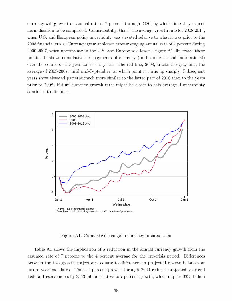
currency will grow at an annual rate of 7 percent through 2020, by which time they expectnormalization to be completed. Coincidentally, this is the average growth rate for 2008-2013,when U.S. and European policy uncertainty was elevated relative to what it was prior to the2008 financial crisis. Currency grew at slower rates averaging annual rate of 4 percent during2000-2007, when uncertainty in the U.S. and Europe was lower. Figure A1 illustrates thesepoints. It shows cumulative net payments of currency (both domestic and international)over the course of the year for recent years. The red line, 2008, tracks the gray line, theaverage of 2003-2007, until mid-September, at which point it turns up sharply. Subsequentyears show elevated patterns much more similar to the latter part of 2008 than to the yearsprior to 2008. Future currency growth rates might be closer to this average if uncertaintycontinues to diminish.

-2

0

2

4

6

8

Per

cent

Jan 1 Apr 1 Jul 1 Oct 1 Jan 1

Wednesdays

2001-2007 Avg.20082009-2013 Avg.

Source. H.4.1 Statistical Release.Cumulative totals divided by value for last Wednesday of prior year.

Figure A1: Cumulative change in currency in circulation

Table A1 shows the implication of a reduction in the annual currency growth from theassumed rate of 7 percent to the 4 percent average for the pre-crisis period. Differencesbetween the two growth trajectories equate to differences in projected reserve balances atfuture year-end dates. Thus, 4 percent growth through 2020 reduces projected year-endFederal Reserve notes by $353 billion relative to 7 percent growth, which implies $353 billion

38

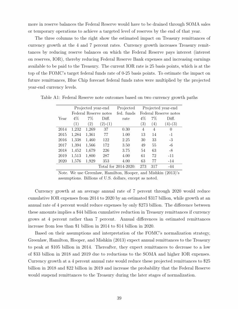
more in reserve balances the Federal Reserve would have to be drained through SOMA salesor temporary operations to achieve a targeted level of reserves by the end of that year.

The three columns to the right show the estimated impact on Treasury remittances ofcurrency growth at the 4 and 7 percent rates. Currency growth increases Treasury remit-tances by reducing reserve balances on which the Federal Reserve pays interest (intereston reserves, IOR), thereby reducing Federal Reserve Bank expenses and increasing earningsavailable to be paid to the Treasury. The current IOR rate is 25 basis points, which is at thetop of the FOMC’s target federal funds rate of 0-25 basis points. To estimate the impact onfuture remittances, Blue Chip forecast federal funds rates were multiplied by the projectedyear-end currency levels.

Table A1: Federal Reserve note outcomes based on two currency growth paths

Projected year-end Projected Projected year-endFederal Reserve notes fed. funds Federal Reserve notes

Year 4% 7% Diff. rate 4% 7% Diff.(1) (2) (2)-(1) (3) (4) (4)-(3)

2014 1,232 1,269 37 0.30 4 4 02015 1,284 1,361 77 1.00 13 14 -12016 1,338 1,460 122 2.25 30 33 -32017 1,394 1,566 172 3.50 49 55 -62018 1,452 1,679 226 3.75 54 63 -82019 1,513 1,800 287 4.00 61 72 -112020 1,576 1,929 353 4.00 63 77 -14

Total for 2014-2020: 273 317 -44Note. We use Greenlaw, Hamilton, Hooper, and Mishkin (2013)’sassumptions. Billions of U.S. dollars, except as noted.

Currency growth at an average annual rate of 7 percent through 2020 would reducecumulative IOR expenses from 2014 to 2020 by an estimated $317 billion, while growth at anannual rate of 4 percent would reduce expenses by only $273 billion. The difference betweenthese amounts implies a $44 billion cumulative reduction in Treasury remittances if currencygrows at 4 percent rather than 7 percent. Annual differences in estimated remittancesincrease from less than $1 billion in 2014 to $14 billion in 2020.

Based on their assumptions and interpretation of the FOMC’s normalization strategy,Greenlaw, Hamilton, Hooper, and Mishkin (2013) expect annual remittances to the Treasuryto peak at $105 billion in 2014. Thereafter, they expect remittances to decrease to a lowof $33 billion in 2018 and 2019 due to reductions to the SOMA and higher IOR expenses.Currency growth at a 4 percent annual rate would reduce these projected remittances to $25billion in 2018 and $22 billion in 2019 and increase the probability that the Federal Reservewould suspend remittances to the Treasury during the later stages of normalization.

39