International and Intercity Trade, and Housing Prices in US

Cities1

Jeffrey P. Cohen2 and Yannis M. Ioannides3

Version: Tufts Brown Bag, November 20, 2017. JEL codes: R00, R11, R15, F40.

1We acknowledge with thanks that we benefited from very insightful conversations with Costas Arko-

lakis, Federico Esposito and Vernon Henderson, from assistance with the data by Albert Saiz, and from

comments by Kevin Patrick Hutchinson, Zack Hawley and other participants at our presentations at the Ur-

ban Economics Association, Minneapolis, November 2016, the ASSA/AREUEA meetings, Chicago, January

2017, participants at C.R.E.T.E., Milos, Greece, July 2017, especially Elias Dinopoulos, and at HULM 2017,

Philadelphia, especially Satyajit Chatterjee and Morris Davis. We are especially grateful to the following

individuals for lending us data: Morris Davis, Roberto Cardarelli, Lusine Lusinyan, and Steven Yamarik.

We remain solely responsible for the content.2Center for Real Estate, Department of Finance, School of Business, University of Connecticut, 2100

Hillside Road, Unit 1041RE Storrs, CT 06269-1041, USA. T: 860-486-1277. F: 860-486-0349. E: Jef-

frey.Cohen@business.uconn.edu http://www.business.uconn.edu/contact/profiles/jeffrey-cohen/3Department of Economics, Tufts University, Medford, MA 02155, USA. T: 617-627-3294. F: 617-627-

3917. E: yannis.ioannides@tufts.edu sites.tufts.edu/yioannides/

1

International and Intercity Trade, and Housing Prices in US Cities

Jeffrey P. Cohen and Yannis M. Ioannides

Abstract

International trade models typically consider countries exchanging goods/services, while ur-

ban models often examine the consequences of domestic trade for city structure. Relatively

little known research synthesizes these to allow for shocks propagating domestically with

both domestic and international trade. One exception is Autor et al. (2013), who examine

how Chinese imports impact US domestic labor markets.

We consider how city-to-city domestic trade and city international exports impact city

Gross Domestic Product (GDP) and housing price growth. We develop a theoretical model

of trading cities, domestically and internationally, and explore its empirical predictions.

We propose and estimate several empirical models. Using instrumental variables (IV), we

identify city-level GDP growth impacts on city house price growth. This equation follows

from imposing spatial equilibrium across cities. A second equation examines how interna-

tional exports from a city, transfers, and domestic shipments impact city-level GDP. We also

consider a third set of equations, which explores how economic integration, domestic and

international, affects city-level GDP growth. In general, our empirical estimation results

confirm the signs/magnitudes predicted by the theory, and imply that labor market shocks

in trading cities affect city-level GDP, which in turn impacts housing prices. Our simulations

show that a shock to international exports has the greatest positive effect on house price

growth, followed by domestic shipments. Our theoretical approach, synthesis of city-level

data, and empirical analysis are completely novel.

2

1 Introduction

An economy’s cities are its vibrant hubs of economic activity and culture. They host a large

and indeed ever increasing share of its population. For a city to function its economy must

provide non-tradeable goods and services, which are required for each city’s survival. Cities

also typically produce tradeable goods, which are exported to the rest of the economy as

well as to the rest of the world, thus allowing their economies to import goods that are

consumed by their population and industries. Production of tradeable and non-tradeable

goods and services typically generates demand for imports of intermediate goods, which are

supplied by other cities in the economy and the rest of the world. Urban economic activity

provides employment and is accommodated by each city’s real estate sector. Real estate

encompasses housing and non-housing structures. Commercial real estate prices and rents,

and housing prices and rents, as well as land values are all key determinants of the cost of

urban production and urban living. Urban economies are profoundly open to domestic and

international competition in their export industries.

Research on housing markets and prices typically looks either at the housing market

alone, or at the housing and labor markets jointly. Other research on international trade,

such as Autor, Dorn, and Hanson (2013), considers the relationship between trade and the

labor markets. Our research reported here is motivated by a very recent literature that links

local housing markets and in international trade. It innovates by bringing into the analysis

some additional but lesser known sources of data, which are critical for understanding urban

economies as open economies. One is the Bureau of Economic Analysis (BEA) data on MSA

GDP, which started in 2001 and is reported annually for 381 US MSAs.4 A second source

is little known data on merchandise exports of different US MSAs to the world economy.5

Furthermore, data on commodity flows from state to state, and within MSA and within

state shipments, allow us to estimate the interactions between trade, on one hand, and labor

and housing markets on the other, at alternative levels of aggregation.6 Other data from

4http://www.bea.gov/newsreleases/regional/gdp metro/gdp metro newsrelease.htm5http://www.trade.gov/mas/ian/metroreport/6Commodity Flow Survey (CFS) is conducted every five years, in years ending in “2” and “7”. Thus,

3

the Brookings Institute also detail MSA exports based on the production location of the

exported products. Adding up the MSA to MSA shipments (including within-MSA), plus

the MSA to each region of the world exports would give us an estimate of overall (domestic

plus international) MSA-level gross sales of traded goods and services.

Availability of trade data, intercity shipments as well as international exports data, allow

us another glimpse at the forces affecting housing costs. For example, a positive shock

to international exports of a particular city translates to shocks to the demand for labor

and housing in that city. Thus, trade data may be brought to bear as a direct proxy of

contemporaneous economic interaction across economic conditions in different cities.

The remainder of this paper is organized as follows. First, we outline a static model of

an economy made up of cities engaged in intercity and in international trade and explore

predictions it offers for structuring an empirical investigation. The model predicts that there

are structural differences across cities of different types in the determination of city GDP

on account of intercity trade, and how GDP growth affects the growth of city-level house

prices. The paper also estimates the respective structural equation for GDP determination.

The empirical implications of spatial equilibrium have been tested before when analyzing

interactions among US cities [c.f. Glaeser et al. (2014)], yet the possibility of structural

differences across US cities have not been analyzed. A third equation derives from modeling

urban growth. The paper next reviews the data and discusses our empirical results.

Our interpretation of the empirical findings is that since trading cities have more channels

through which an employment shock can be absorbed, there is much less of an impact that is

passed through to the housing markets and therefore house price growth may be much more

the two latest ones are for 2002, 2007 and 2012. As Duranton et al. (2014) clarify, the CFS divides the

continental US into 121 CFS regions, each an aggregation of adjacent counties. The Duranton and Turner

sample consists of the 66 such regions organized around the core county of a us metropolitan area. CFS

cities are often larger than the corresponding (consolidated) metropolitan statistical areas. For instance,

Miami–Fort Lauderdale and West Palm Beach–Boca Raton in Florida are two separate metropolitan areas

according to the 1999 US Census Bureau definitions but they are part of the same CFS region. In our

analysis, we create correspondence between CFS cities in the years 2007 and 2012 with the 2002 CFS city

definitions, leading to 76 cities in each of these three years.

4

insulated. To the best of our knowledge, the paper’s approach is completely novel; we are

unaware of any previous research that synthesizes the intercity trade data, city-level housing

price data, and international exports data, nor of their role in estimation of city GDP.

2 Literature Review

There is relatively little literature that emphasizes empirically the structural implication of

intercity trade. Pennington-Cross (1997) focuses on the development of an exports price

index, in the context of estimating external shocks to a city’s economy. There are several

later applications of this index, including Hollar (2011), which is a study on central cities

and suburbs; Larson (2013), which considers housing and labor markets in growing versus

declining cities; and Carruthers et al. (2006) on convergence. Most of these papers use

a similar earlier data set on exports from the 1990s from the International Trade Agency

(ITA), which was discontinued prior to 2000. A new exports data set has been released by

the ITA beginning in 2005, although one drawback of that data source is that it is based on

origin of shipments rather than origin of production.

A second but smaller strand of literature uses actual export quantities as control vari-

ables, with the exports data being the central focus of the paper for only some of these

industries. For others they are not the primary focus of the papers (they are merely used as

controls). These include Lewandowski (1998), which considers economies of scale of exports

in MSAs, using the earlier exports data set from the ITA. Ferris and Riker (2015) study

the relationships between exports and wages, using the more recent data set on exports, but

focus on measurement and data construction aspects. Braymen et al. (2011) examine R&D

and exports, using a somewhat limited, firm level database on exports from the Kauffman

Foundation, and control for R&D activity in the metro area. Finally, Vachon and Wallace

(2013) use the exports data to assess how globalization affects unionization in 191 MSAs.

Finally, a more recent paper by Li (2017) uses a very rudimentary empirical analysis to

motivate her theoretical model and simulations for US cities that describes the relationship

between house prices and comparative advantage. The theory is the primary focus of that

5

paper. Our understanding of export-oriented cities would benefit from further analytical and

empirical attention, in view of the sparseness of published research integrating theoretical

underpinnings with rigorous empirical modelling on house prices, GDP, and exports at the

MSA level, together with the limitations of some of the other exports data sources.

3 Intercity Trade and the Housing Market

Drawing on standard approaches for modeling interactions among systems of cities [ Desmet

and Rossi-Hansberg (2015); Ioannides (2013) ], the present paper describes an economy as

being made up of cities of different types. Types differ according to the number and types of

final goods produced, or whether or not they produce only intermediate goods and import

all final goods. This literature originated by Henderson (1974). The present paper draws

from Ioannides (2013), Chapter 7, which develops a variety of rich urban structures in a

static context and ibid., Chapter 9, in a dynamic one. Both approaches impose intracity

and intercity spatial equilibrium. In the case of the static model, manufactured goods

may be either produced locally or imported from other cities. Manufactured goods are

produced using raw labor and intermediate goods interpreted as specialized labor, which are

themselves produced from raw labor, using increasing returns to scale (IRS) technologies.

In the case of the dynamic model, manufactured goods are produced using raw labor and

intermediate goods interpreted as specialized labor, which are themselves produced from raw

labor, using IRS technologies, and physical capital. In either case, those goods are combined

locally to produce a final good that may be used for either consumption or investment.

Urban functional specialization, rather than sectoral, as articulated by Duranton and Puga

(2005), also leads to structural differences. In other words, certain economic functions,

like management, research and development and corporate headquarters may be located in

different places than manufacturing. With industrial specialization and diversification being

important features of urbanized economies, cyclical patterns in urban output differ across

cities, and so do patterns in the variations of employment and unemployment [Rappaport

(2012); Proulx (2013)].

6

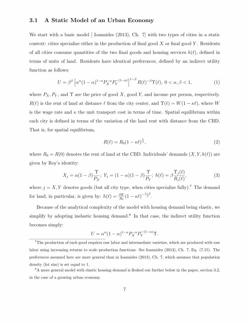
3.1 A Static Model of an Urban Economy

We start with a basic model [ Ioannides (2013), Ch. 7] with two types of cities in a static

context: cities specialize either in the production of final good X or final good Y . Residents

of all cities consume quantities of the two final goods and housing services h(ℓ), defined in

terms of units of land. Residents have identical preferences, defined by an indirect utility

function as follows:

U = ββ[αα(1− α)1−αP−α

X P−(1−α)Y

]1−βR(ℓ)−βΥ(ℓ), 0 < α, β < 1, (1)

where PX , PY , and Υ are the price of good X, good Y, and income per person, respectively.

R(ℓ) is the rent of land at distance ℓ from the city center, and Υ(ℓ) = W (1− κℓ), where W

is the wage rate and κ the unit transport cost in terms of time. Spatial equilibrium within

each city is defined in terms of the variation of the land rent with distance from the CBD.

That is, for spatial equilibrium,

R(ℓ) = R0(1− κℓ)1β , (2)

where R0 = R(0) denotes the rent of land at the CBD. Individuals’ demands (X,Y, h(ℓ)) are

given by Roy’s identity:

Xj = α(1− β)Υ

PX

; Yj = (1− α)(1− β)Υ

PY

; h(ℓ) = βΥj(ℓ)

Rj(ℓ), (3)

where j = X,Y denotes goods (but all city type, when cities specialize fully).7 The demand

for land, in particular, is given by: h(ℓ) = βWR0

(1− κℓ)−1−ββ .

Because of the analytical complexity of the model with housing demand being elastic, we

simplify by adopting inelastic housing demand.8 In that case, the indirect utility function

becomes simply:

U = αα(1− α)1−αP−αX P

−(1−α)Y Υ.

7The production of each good requires raw labor and intermediate varieties, which are produced with raw

labor using increasing returns to scale production functions. See Ioannides (2013), Ch. 7, Eq. (7.15). The

preferences assumed here are more general than in Ioannides (2013), Ch. 7, which assumes that population

density (lot size) is set equal to 1.8A more general model with elastic housing demand is fleshed out further below in the paper, section 3.2,

in the case of a growing urban economy.

7

Income per person in each city type is defined as total income per person, which consists

of labor income plus land rental income divided by city population, which is denoted by

NX , NY for each type of city. For the simpler model, populations in each city type, Nj,

j = X,Y, and physical city sizes, ℓj =(Nj

π

) 12 imply an expression for net labor supply:

Hc(Nj) =∫ (Nj

π

) 12

02πℓ(1− κ′ℓ)dℓ = Nj(1− κ′N

12j ), (4)

where κ′ = 32π

12 . Assuming that the value of land at the fringe of the city is given by the

agricultural rent, Ra,j, allows us to solve for physical city size. That is, we have:

Rj(ℓ) = Ra,j = R0,j

(1− κ′ℓ

)W, (5)

where W denotes the nominal wage rate. From this and the previous equations, we may

solve for R0,j and ℓj as functions of (Nj, Ra,j). Land rental income is given by

Yj,land =

1

Nj

∫ ℓj

02πℓRj(ℓ)dℓ =

1

2κ′WN

1/2j . (6)

Labor income per person, Yj,labor is equal to wage rate times the labor supply net of

commuting costs (which are expressed in terms of time), on the supply side, and to the value

of sales of the good a city is specializing in, on the demand side, which in turn is spent on

both final goods. Thus, allowing for transfers from elsewhere in the economy, and denoting

net transfers per person into city j by Tj, total income per person is equal to labor income

per person, Yj,labor, plus land rental income per person, Y

j,land, plus transfers per person,

Tj:

Υj = Yj,land + Y

j,labor + Tj. (7)

We note that GDP per person is observable and may be used in the place of Υj. Transfers

account for income that originates outside the particular city, but may depend on city de-

mographics. Also, we experiment with income per employee, which is appropriate because

congestion is associated with travel to work.

Because of complexity of analytical expressions, the assumption is often made that land

income is redistributed equally among all residents rather than being earned by absentee

landlords. In such a case, income net of commuting and land costs may be expressed in terms

8

of population and the price of the good in which the city specializes; see below [Ioannides

(2013), p. 315]. Because of intraurban transportation costs, which take the form of time,

labor supply, that is available labor minus commuting costs, depends upon the geographic

complexity of the city. E.g., with linear commuting costs, assumed above, K(ℓ) ≡ κℓ, and

inelastic demand for land, net labor supply is given by (4) [ibid., p. 300, eq. (7.2)]. This

expression is more complicated in the exact case of our model where housing demand is

elastic, or when city geography is more complicated. Thus, GDP supply per person in a city

of type j is given by 1NjF (Hc(Nj)), where F (·) denotes the aggregate production function

and Hc(Nj) denote the net labor supply in city j given by (4). Under the assumptions of

Ioannides (2013), Chapter 7, GDP supply per person in city j, gross of transfer income, is

given by:

Υj = BjδjPjN1−ujσ−1

j (1− κ′N1/2j )

σ−ujσ−1 , j = X,Y, (8)

where Bj is a function of technology parameters, δj = 1 + (nj − 1)τσ−1 a function of the

number of cities of each type and intercity iceberg shipping costs parameter for intermediates,

uj is the elasticity of raw labor in the Cobb-Douglas production function of good j, 1 − uj

the elasticity of the CES aggregate of intermediates used in production of each good, and

σ the elasticity of substitution among the intermediates. This particular result serves to

underscore that city geography, and more generally congestion, have complex effects on city

GDP supply per person.

For national equilibrium in an economy consisting of nX cities of type X and nY cities

of type Y, total population N is allocated to all cities,

nXNX + nYNY = N . (9)

In the absence of shipments to the rest of the world (ROW), all exports of good X are

purchased by cities of type Y , and all exports of good Y are purchased by cities of type X,

the total spending on good Y by all cities is equal to the total spending on good X, where

X,Y denote, respectively, the production of good X, good Y by each city of the respective

type. That is:

(1− β)(1− α)nXXPX = (1− β)αnY Y PY . (10)

9

Spatial equilibrium among cities is expressed as equalization of utility across cities of different

types. Adopting Ioannides (2013), section 7.5, with the expression for income per person in

we have that:

UX = CXδ1−uXσ−1

X

(PX

PY

)1−α

N1−uXσ−1

X (1− κ′N1/2X )

σ−uXσ−1 ; (11)

UY = CY δ1−uYσ−1

Y

(PX

PY

)−α

N1−uYσ−1

Y (1− κ′N1/2Y )

σ−uYσ−1 , (12)

where CX , CY are suitably defined constants, and δj’s reflect shipping costs for intermediates

and the numbers of cities of each type.9 Whereas it would be straightforward to work with

these utility functions in order to obtain spatial equilibrium conditions, we postpone such

an exercise for the more general model we develop next.

Working from (10) we may express aggregate demand in X− type cities per person in

terms of total spending on good X by all other cities per person. This may be proxied by

shipments per capita SX from cities of type X to all other cities, SX = (1− β)α nY

nXNXY PY ,

plus the value of per capita shipments to the rest of the world (ROW), exX from a city

of type X, plus per capita transfers from the rest of the domestic economy, TX . That is,

respectively for each city type X, Y , we have:

ΥX = (1− β)αnY

nXNX

Y PY + TX + exX ; ΥY = (1− β)(1− α)nX

nYNY

XPX + TY + exY . (13)

This will be generalized further below to allow for imports from the ROW. We note that the

terms nY

nXNXY PY ,

nX

nY NYXPX may be directly proxied by the value of shipments from each

city to all other cities.

At a first level of approximation, we may ignore city type10 and use Eq.’s (13) to motivate

a single regression equation for each city that expresses the aggregate demand for GDP per

capita in city j in terms of shipments to other cities, Sj, per capita transfers j, Tj, and

exports by city j, exj, to the rest of the world:

Υj = γ1Sj + γ2Tj + γ3 exj. (14)

9Iceberg shipping costs for final products are reflected on the equilibrium terms of trade; see Ioannides

(2013), Section 7.5.10City types are hard to assign, because only a small share of city employment may be reliably linked to

a city’s export industries for most cities. See Ioannides (2013), Chapter 7.

10

This equation expresses a key feature of the system of cities model: GDP is determined by

equilibrium in the goods markets, via the interaction of each city with all other cities, and

equilibrium within each city housing market, which enters the definition of Υj, aggregate

income per person. Each city supplies goods and services to all other cities and buys goods

and services from them. Since in an economy like that of the US cities are very open

(within the domestic economy) economic entities — in terms of movement of commodities,

of people and of knowledge flows — city GDP determination is a critical relationship, much

like national income determination of internationally open economies. Here all intercity

transactions are expressed as trades in the national currency. It readily follows from (7) and

(14) that the conditions γ2 = γ3 = 1 are testable empirically.

While the model incorporates spatial equilibrium within each city, the urban system is in

equilibrium if identical individuals are indifferent among all city locations. Equalizing utility

across all cities at all times yields the inter-city spatial equilibrium condition. Taking first

differences allows us to define the growth rate of land value, R0,j, for each city relative to a

reference urban land value growth rate for the entire system of cities, R0,n, in terms of the

growth rate of the price index for city j, Pj, relative to an urban price index, Pu, and the

growth rate of per capita income relative to the growth rate of national per capita income,

Υn:

GRt+1,t(R0,j)−GRt+1,t(R0,n) = [GRt+1,t(Pj)−GRt+1,t(Pu)] + [GRt+1,tΥj −GRt+1,t(Υn)] .

(15)

Eq. (14–15) can be taken to the data. Both these equations are derived using a simplified

framework for the purpose of demonstrating the empirical potential of the model. Next, we

introduce a more general model for individuals’ behavior which implies a more complicated

spatial equilibrium condition, in which (15) may be nested.

11

3.2 A Model of Urban Economic Integration, Specialization and

Economic Growth

The exposition that follows extends the main model in Ioannides (2013), Chapter 9, in order

to allow for international trade.11 It is a dynamic model that allows for differences across

cities in terms of city-specific total factor productivities, which will be discussed further

below, and of congestion parameters κi. It assumes that individuals are free to move across

cities, thus spatial equilibrium is imposed, that is: individuals are indifferent as to where

they locate. That is, individuals’ lifetime utilities are equalized across all cities. This implies

in turn conditions on intercity wage patterns. Similarly, if capital is perfectly mobile, it will

move so as pursue maximum nominal returns and in the process equalize them across all

cities.

This section aims at obtaining, first, a more general expression for spatial equilibrium

and its implications for the growth rate of the price of land (or housing), and second, more

general expressions for the growth rate of city GDP for cities engaging in domestic trade as

distinct from those engaging in international trade.

A number of individuals Nt are born every period and live for two periods. The econ-

omy has the demographic structure of the overlapping generations model. We assume that

individuals born at time t work when young, consume nonhousing and housing out of their

their labor income net of their savings, (C1t, G1t), and consume again when they are old,

(C2t+1, G2,t+1) respectively. We assume Cobb-Douglas preferences over first- and second-

period consumption for the typical individual,

Ut = S∗[C1−β1t Gβ

1t]1−S[C1−β

2t+1Gβ2,t+1]

S, 0 < S < 1, (16)

where S∗ ≡ [S1−βββ]−S[(1− S)1−βββ]−(1−S), and parameter S satisfies 0 < S < 1.

Net labor supplied by the young generation in a particular city at t is given by Ht =

Nt

(1− κN

12t

), with Nt the number of the members of the young generation in a particular

11This main model of Ioannides, Ch. 9, constitutes an original adaptation of Ventura (2005)’s model of

global growth to the urban structure of a national economy by building on key features of Ioannides (2013),

Ch. 7.

12

city at t, κ ≡ 23π− 1

2κ′, and κ′ the time cost per unit of distance traveled.

If Wt denotes the wage rate per unit of time, spatial equilibrium within the city obtains

when labor income net of land rent is independent of location. This along with the assump-

tion that the opportunity cost of land is 0, and therefore the land rent at the fringe of the

city is also equal to 0, yields an equilibrium land rental function as per Chapter 7, Ioannides

(2013). It declines linearly as a function of distance from the CBD and is proportional to the

contemporaneous wage rate, Wt. It is convenient to close the model of a single city and to

express all magnitudes in terms of city size. WE again assume that all land rents in a given

city are redistributed to its residents when they are young, in which case total rental income

may be written, according to (6), in terms of the number of young residents as 12κWN

32t .

This yields first period net labor income per young resident, after redistributed land rentals

and net of individual commuting costs, of(1− κN

12t

)Wt. With a given wage rate, individual

income declines with city size, other things being equal, entirely because of congestion. But,

there are benefits to urban production which are reflected on the wage rate.

Let Rt+1 be the total nominal return to physical capital, Kt+1, in time period t + 1,

that is held by the member of young generation at time t. The indirect utility function

corresponding to (16) is:

V = RS(1−β)t+1 P

−(1−S)βG,t P−Sβ

G,t+1

(1− κN

12t

)Wt, (17)

where we assume that the price of consumption is normalized to 1. We assume that capital

depreciates fully in one period. The young maximize utility by saving a fraction S of their

net labor income. The productive capital stock in period t + 1, Kt+1, is equal to the total

savings of the young at time t. Therefore, previewing our growth models, we have: Kt+1 =

SNt

(1− κN

12t

)Wt.

We refer to the case where capital and labor are free to move as economic integration.

With economic integration, industries will locate where industry productivities, the industry-

specific TFP functions ΞJt’s,12 are the most advantageous, and capital will seek to locate

12See Appendix A for details on the specification of the urban production structure and clarification of

the role of the industry-specific TFP functions ΞJt’s.

13

so as to maximize its return. Unlike the consequences of economic integration as examined

by Ventura, op. cit., where aggregate productivity is equal to the most favorable possible

in the economy, here urban congestion may prevent industry from locating so as to take

greatest advantage of locational factors. Put differently, free entry of cities into the most

advantageous locations may be impeded by competing uses of land as alternative urban

sites, at the national level. However, utilities enjoyed by city residents at equilibrium do

depend on city populations, and therefore, spatial equilibrium implies restrictions on the

location of individuals. We simplify the exposition by assuming that all cities have equal

unit commuting costs κ.

We assume that cities specialize in the production of tradeable goods. We examine the

case when each specialized city also produces intermediates that are used in the production

of the traded good. Let QXit, QY jt denote the total quantities of the traded goods X,Y

produced by cities i, j, that specialize in their production, respectively. The formulation is

symmetrical for the two city types, and therefore, We work with a city of type X.

The canonical model of an urban economy assumes that capital is free to move. Thus,

nominal returns to capital are equalized across all cities. The model assumes that individuals

are free to move, which in the context of our two-overlapping generations requires that

lifetime utility is equalized across all cities. By using these conditions simultaneously, we

obtain a relationship between housing prices, consumption good prices and nominal incomes

across cities, which may be taken to the data.

3.2.1 Spatial Equilibrium

WE suppress redundant subscripts and write for the nominal wage and the nominal gross

rate of return in an type−X city:

WXt = (1− ϕX)PXQX

HX

, RXt = ϕXPXQX

KX

, (18)

where PX denotes the local price of traded good X, which is expressed in terms of the local

price index, the numeraire, which is equal to one in all cities. We also assume initially that

there are no intercity shipping costs for traded goods. With economic integration, the gross

14

nominal rate of return is equalized13 across all city types, that is:

Rt = RXt = RY t.

Spatial equilibrium for individuals requires that indirect utility, (17), be equalized across

all cities. In view of free capital mobility, spatial equilibrium across cities of different types

requires that:

P−(1−S)βG,X,t P−Sβ

G,X,t+1

(1− κN

12Xt

)WXt = P

−(1−S)βG,Y,t P−Sβ

G,Y,t+1

(1− κN

12Y t

)WY t. (19)

By taking logs we have:

−(1− S)β lnPG,X,t − Sβ lnPG,X,t+1 + ln(1− κXN

12Xt

)+ lnWXt

= −(1− S)β lnPG,Y,t − Sβ lnPG,Y,t+1 + ln(1− κYN

12Y t

)+ lnWY t. (20)

Just as in the previous section, this allows us to obtain a condition for spatial equilibrium

within each city, which is written directly in terms of labor earnings. Earnings here are

expressed in terms of real city output, so we deflate them in terms of a city price index.

Thus, spatial equilibrium implies:

GRt+1,t(PG,j)−GRt+1,t(PG,n) = −1− S

S

[GRt+1,t(Pj)−GRt+1,t(Pj,u)

]

+1

Sβ[GRt+1,tΥj −GRt+1,t(Υn)] + ln

(1− κXN

12Y t

)− ln

(1− κnN

12nt

). (21)

We note that we have imposed spatial equilibrium The last two terms in the right hand side

of the above proxy for spatial complexity, regulation, and housing supply factors. Clearly,

condition (15), obtained with a simpler behavioral model, may be nested within (21). In

particular, the coefficient of GRt+1,t(Pj) − GRt+1,t(Pj,u), the growth rate of the city price

index relative to a national average, is predicted to be positive; the coefficient of GRt+1,tΥj−

GRt+1,t(Υn), the growth rate of income per capita relative to a national average is predicted

to greater than 1.

13As Fujita and Thisse (2009), p. 113, emphasize, while the mobility of capital is driven by differences

in nominal returns, workers move when there is a positive difference in utility (real wages). In other words,

differences in living costs matter to workers but not to owners of capital.

15

3.2.2 Intercity Trade and Determination of City GDP

Next we derive expressions for real incomes in different city types in an economy with city

specialization in tradeable goods which are combined in every city to produce a composite

good which is used for consumption and investment. For a city of type X real income is

equal to the value of the output of the good in which that city specializes, PXQX , and

PYQY , for a city of type Y. From the definition of the numeraire, in every city: PX =

αα(1 − α)1−α(PX

PY

)1−α. By using the condition for spatial equilibrium, we may obtain an

expression for the terms of trade, the price ratio, from which we may obtain an expression

for the real income of a type X city:

QXαα(1− α)1−α

(PX

PY

)1−α

= α∗XQ

αXQ

1−αY

(NXit

NY it

)1−α

,

where α∗X = αα(1 − α)1−α

(1−ϕY

1−ϕX

)1−α. Introduction of iceberg shipping costs for tradeable

goods lead a trivial modification of this condition. The real income of a city specializing in

good X, Xt, is expressed in terms of city populations of both types of cities, (NX , NY ), total

capital in the economy, Kt, and parameters as follows:

Xt = NX

(Kt

N

)αµXϕX+(1−α)µY ϕY

, (22)

where the auxiliary variable NX is defined as a function of city sizes and parameters:

NX(NX , NY ) ≡ α∗XΞtN

αµX+1−αX

(1− κN

12X

)αµX(1−ϕX)

N(1−α)µY −(1−α)Y

(1− κN

12Y

)(1−α)µY (1−ϕY )

,

(23)

and the function Ξt, defined as a transformation of the industry-specific TFP functions

ΞXt, ΞY t14:

Ξt ≡ ΞαXtΞ

1−αY t

(ϕX

1− ϕX

)αµXϕX(

ϕY

1− ϕY

)(1−α)µY ϕY(1− αϕX − (1− α)ϕY

αϕX + (1− α)ϕY

)αµXϕX+(1−α)µY ϕY

.

(24)

14See Appendix A for details on the specification of the production structure and the details of how the

industry-specific TFP functions enter. The TFP function Ξt is the counterpart for the integrated economy

of Ξ∗t , defined in Ioannides (2013), Ch. 9, for the autarkic cities. The industry TFP functions enter Ξt with

the same exponents as in Ξ∗t , but the shift factors differ.

16

The counterpart of (22) for PYQY , the real income of a city specializing in good Y, is

given by:

Yt = NY

(Kt

N

)αµXϕX+(1−α)µY ϕY

, (25)

where α∗Y = αα(1− α)1−α

(1−ϕX

1−ϕY

)α,

NY (NX , NY ) ≡ α∗Y ΞtN

αµX−αX

(1− κN

12X

)αµX(1−ϕX)

N(1−α)µY +αY

(1− κN

12Y

)(1−α)µY (1−ϕY )

.

(26)

Eq. (22) and (25) define city income for cities of type X and of Y , respectively, as

functions of the economy wide capital per person, Kt

N, and of NX ,NY , which are functions

of populations of both city types, of economy wide TFP, Ξt, defined in (24) above, and of

parameters.

Taking logs of both sides of (22) and (25) and subtracting the second from the first, we

have:

lnXt − lnYt = lnNX − lnNY . (27)

By using the definitions of NX ,NY , in (23), (26), the rhs above becomes: lnα∗X − lnα∗

Y +

lnNX − lnNY .

3.2.3 Growth of Integrated Cities

By taking logs and time-differencing, we may express the growth of income of income for

a particular city in terms of constants and the difference in the growth rate of a city of a

particular type from that of the average city, and of the growth rate of aggregate capital.

That is, we have for growth in income for type−X and type−Y cities,

GR(XX,t) = lnXt+1 − lnXt, GR(ΥY,t) = lnYt+1 − lnYt

respectively:

GR(XX,t) = GR(Ξt) + (αµX + 1− α)GR(NX,t) + ((1− α)µY − (1− α))GR(NY,t)

+(αµXϕX + (1− α)µY ϕY )GR(Kt)− (αµXϕX + (1− α)µY ϕY )GR(Nt)

17

−αµX(1− ϕX)κ[N12X,t+1 −N

12X,t]− (1− α)µY (1− ϕY )κ[N

12Y,t+1 −N

12Y,t]. (28)

GR(ΥY,t) = GR(Ξt) + (αµX − α)GR(NX,t) + ((1− α)µY + α))GR(NY,t)

+(αµXϕX + (1− α)µY ϕY )GR(Kt)− (αµXϕX + (1− α)µY ϕY )GR(Nt)

−αµX(1− ϕX)κ[N12X,t+1 −N

12X,t]− (1− α)µY (1− ϕY )κ[N

12Y,t+1 −N

12Y,t]. (29)

These growth equations may be rewritten in terms of the difference between the growth rate

of an individual city from that of the average city.

A number of remarks are in order in taking these equations to the data. First, the as-

sumptions of the model imply that the term GR(Ξt) in the RHS of (28) may be treated

as a total factor productivity growth rate, i.e., a Solow residual. Furthermore, it is not

city-specific. Second, since the growth rate of the economy’s aggregate physical capital,

term GR(Kt), is also common to all cities, it could be instrumented by means of the na-

tional nominal interest rate. Third, the coefficient of the aggregate population growth rate,

(αµXϕX + (1− α)µY ϕY ), is the same as that of growth rate of the economy’s aggregate phys-

ical capital. Therefore, by following our approach above and expressing growth in income

per person relative to the economy’s average, where as before for a city of type X the terms

associated with cities of type Y serve as proxies for the average economy, the only remaining

of the growth rate terms is the growth rate of a city’s population relative to the national

average. The other remaining terms express the evolution of a city’s spatial complexity,

relative to the economy’s average. It is these predictions that we take to the data.

3.2.4 Growth of Autarkic Cities

The growth equations obtained above, (28) and (29), follow from the assumption of national

economic integration and specialization. To see this we may contrast with growth in autarkic

cities. Working from Eq. (9.15), Ioannides (2013), p. 414, we have that the growth rate

of income per person may be expressed in terms of the same (log)linear combination of the

TFP growth rates of the city’s different industries, α ln ΞXt+(1−α) ln ΞY t, and in addition,

the growth rate of the respective effective labor supply, and of the aggregate physical capital

18

in that city. That is:

GR(Υaut,jt) = αGRt,t+1(ΞX) + (1− α)GRt,t+1(ΞY ) + (µϕ+ υ)GRt,t+1(Kj,t)

+(µ(1− ϕ)− υ)GRt,t+1(Hc(Njt)). (30)

We note that this result predicts that other than the presence of a linear combination of

the TFP growth rates of the city’s different industries the coefficient of the remaining term,

GRt,t+1(Hc(Nt)) the city’s effective population growth rate, is predicted to be positive. See

Ioannides (2013), p.417. We note that whereas in Eq. (28) and (29), Kt denotes aggregate

physical capital in the economy, here Kj,t denotes physical capital for city j at time t.

The urban system of a modern market economy contains cities of different types (Ioan-

nides (2013), Ch. 7) which are in varying degrees integrated into the national and the inter-

national economy. Therefore, city growth rates could in general be described by (28), with

(30) allowing development of over-identifying restrictions. Comparing city output growth

for cities engaged in intercity trade, (28), with that for autarkic cities, (30) suggests that

modeling specifically cities’ trading outside the system of cities with the rest of the world,

is likely to yield expressions for the determination of city GDP that differ from those where

there is no international trade. Appendix B details a modification of the model to account

for international trade along with intercity trade.

3.3 Consequences for Growth Regressions

The spatial equilibrium condition, which expresses arbitrage, turns out to have major im-

plications for urban growth equations in the context of economic integration. This follows

from a comparison between the growth equation for autarkic cities with no free movement

of labor, which is derived here from from Ioannides (2013), Eq. (9.15), as Eq. (30), with the

respective one for cities engaged in intercity trade, Eq. (28), and the one for cities engaged

in intercity and international trade, Eq. (37).

The consequences of spatial equilibrium for urban growth regression has been emphasized

recently by Hsieh and Moretti (2017). They show empirically that spatial equilibrium intro-

duces dependence among city growth rates, which makes the contribution of a particular city

19

to aggregate growth differ significantly from what one might naively infer from the growth

of the city’s GDP by means of a standard growth-accounting exercise. They show that the

divergence can be dramatic. E.g., despite some of the strongest rate of local growth, New

York, San Francisco and San Jose were only responsible for a small fraction of U.S. growth

during the study period. By contrast, almost half of aggregate US growth was driven by

growth of cities in the South. This divergence is due to the fact that spatial equilibrium

imposes restrictions on city-specific TFP growth rates.

However, to the best of our knowledge, no previous literature has dealt explicitly with

international along with intercity trade. The theory outlined here predicts structural dif-

ferences in growth regressions across cities with different roles in the urban system. This

would be critical if we were to perform a classic Solow residual analysis by working from city

output in terms of factor inputs, a point forcefully made by Hsieh and Moretti (2017). It is

clear from (22) that a portion of the contribution of capital and that of labor in its entirety

are subsumed in the auxiliary variables (Xt,Yt)), defined in (23) and (23) above. This is also

confirmed by contrasting with (30), the expression for the growth rate of autarkic cities. In

work currently in progress, we plan to estimate the growth equations by also including data

on capital accumulation.

Another question that would require a modification of the growth model would be to

consider how anticipated growth rates on housing prices may hamper city growth. Because

of varying housing supply restrictions across various US cities, Glaeser and Gyourko (2017)

argue that the local and state control of land use regulations may be quite important in this

regard and may also be responsible for spatial variation in housing equity accumulation by

US households. Doherty (2017) dramatizes this point by invoking Hsieh and Moretti (2017),

arguing that local land-use regulations reduce the United States’ GDP by as much as $1.5

trillion a year, or about 10%. As we discuss in section 6.2, our model and estimation results

are consistent with the arguments proposed Glaeser and Gyourko and Hsieh and Moretti.

20

4 Overview of Data

We have assembled data from a variety of sources, which we use as comprehensively as

possible to investigate the relationship between intercity and international trade, on the one

hand, and the local housing market, on the other. We describe these data to provide an

overall view of the empirical resources we bring to our approach.

The following major sources of data are available to us. We combine some of these into a

dataset for 78 cities for the years 2002, 2007, and 2012 (an unbalanced panel), for estimation

of the GDP determination equation 14. We develop a separate dataset for 96 cities annually

for a 10 year period, for estimation of the house price growth equation 21. Finally, we

combine data for 367 MSAs, split into small versus large cities, over a 5 year period, to

estimate the GDP growth equations 28 and 29. Specifically:

• Equation 14: Data from various sources merged, for 78 cities, 2002, 2007, 2012 (an

unbalanced panel) . Data on city-level domestic shipments for 2002, 2007, 2012 for

78 cities are from the Commodity Flows Survey, BTS. We impute transfers via an

procedure based on equation (7), as the residual of land and labor income, which we

need to instrument in estimating GDP determination. Labor income is derived from

BEA data; land income is based on equation (6), i.e., the product of commuting costs,

wages, and square root of employment; these data are from BEA. Annual international

exports by 377 MSAs, 2003-2012, from Brookings for: agriculture; educational services,

medical services and tourism; engineering; finance; general business; IT; manufacturing

and mining. Aggregate to obtain total MSA exports, and then merged into the 78

city definitions. The following instruments are used for estimating the IV models in

equation 14: Domestic Shipments Instruments are based on the planned highway rays,

lagged 30 years (Baum-Snow, 2007), defined as the number of highway segments that

pass into and/or out of a central city; 30 year lagged miles of completed highway

miles (both from Baum-Snow, 2007); and the difference between national population

and city population from the Census Bureau. Transfers are instrumented with real

unemployment receipts per capita (as in Gruber, 1997), with data obtained from BEA.

21

For international exports, we assume demand for exports exogenous to a city (i.e., city

is small with respect to the rest of the world).

• For Equation 21: Data for 96 cities for 10 years (2003-2012), are obtained by merging

the following: House prices, 1996-2013, 363 MSAs, from the FHFA; given limited

geographical detail in the CPI data we use regional data for the four Census regions

annually, from BLS. There are MSA-level data for 26 MSAs, annually, but to preserve

a larger sample, we use regional data, and we assume these regional prices exogenous

to a particular city. Similarly, all urban cities CPI is exogenous to a particular city.

MSA-level GDP data, and MSA employment data, are obtained from BEA. Regarding

instruments for equation 21, for the MSA employment data we utilize Saiz–Wharton

data (house supply elasticity, unavailable land, Wharton regulation index), and MSA

population, ∼ 250 MSAs (Saiz, 2010). Instruments for MSA GDP growth minus

national GDP growth are given as difference in MSA cancer deaths growth and national

cancer deaths growth, 2003-2012, 96 MSAs, from the Centers for Disease Control.

• Equations 28 (large cities) and 29 (small cities), 180 and 187 MSAs, respectively, annual

data for 2006-2010: The variables in these equations include MSA-level GDP (from

BEA), state-level TFP (from Yamarick), MSA Employment net of commuting time

(calculated from BEA data), federal funds rate (for large cities; from Federal Reserve);

state-level manufacturing capital stock (for small cities; derived from investment data

from Census Bureau’s ASM Geographical Area Series), highway capital stock (for

small cities; derived from investment data from Census Bureau’s State Government

Finances). We also include year and region fixed effects in these equations.

4.1 International versus Intercity Trade Flows

Here we discuss some features of intercity shipments data for 2002, 2007 and 2012, using

the 76 city definitions we generate from the 2002 CFS. We have matched the roughly 377

MSAs with exports data from the Brookings data source. Exports from city j to the rest

22

of the world are obtained from the Brookings Institution15. Since there are fewer cities in

the CFS than in the Brookings dataset, many of the exporting MSAs have been combined

manually in several instances into a number of broader CFS city definitions. This process

was tedious and runs into the difficulty of changing MSA definitions and different numbers of

MSAs across the different waves of the data. Because of these issues, we have approximately

76 cities that we are able to use from the CFS, and we match the data from the 2007 and

2012 CFS, with the MSA GDP and exports data, to roughly 76 city definitions in the 2002

CFS.

We note that the ratio of MSA international exports, defined as international shipments,

to domestic exports shipments is generally highest in coastal cities, and lower in inland cities.

This of course accords with intuition, given that, in general, water shipping is less costly

than other modes. Washington DC is an outlier, because apparently it ships very little

domestically (the government services it produces are not tradeable), and also because it

has approximately 27% of the educational services, medical services, and tourism industry

exports. While it is possible to break down the exports by reported industry, it is not easy

to do so for domestic shipments due to sparseness of the data in some locations that caused

the Census Bureau not to disclose the data.

The comparison of the ratio of exports to domestic shipments across the three different

years is interesting. For 2007, the mean value of the ratio is 0.2047 and its standard deviation

0.7704. These values imply a coefficient of variation of 3.76. In contrast, both mean and

standard deviation are at 0.2738 and 1.2421, respectively, greater for 2012. However, the

coefficient of variation at 4.5357 is also greater, and the range of values has widened. In

other words, it appears as if U.S. cities on average have become more international export

driven over time. There is also a greater spread in cities’ export ratio. Some have become

much more export intensive while others have become much less export intensive, where the

shift is somewhat greater on the higher end of the distribution.

15http://www.brookings.edu/research/interactives/2015/export-monitor#10420

23

4.2 Descriptive Statistics

Table 1a presents descriptive stats for the data used in the regressions for equations 7 an 12.

In Table 1a, the average GDP per job is approximately $47,900, with the average transfer

equal to about $117,000 and the average domestic sales per job approximately $59,000.

In Table 1b, during the period 2002-2012, the average annual land rent growth per job is

negative for both the MSA level and the overall urban total, with the MSA level being more

negative than the overall. This negative average may be attributable to the Great Financial

Crisis that began in late 2007. The GDP growth rate is approximately 3.7% annually during

this period of 2002-2012, while the CPI growth rate is approximately 2.3%. In Table 1c,

the average annual MSA-level GDP growth rate per job in the years 2003-2012 was about

3.57%, while the average cancer death rate per job was 0.43%. Finally, in Table 1d, the

average MSA nominal GDP was approximately $66.6 billion, with 537,000 ”effective” jobs

in ”large” cities and 61,000 ”effective” jobs in ”small” cities.

5 Estimations

For the determination of city GDP, eq. (14), we use per-capita sales data by each city to

other domestic cities, which are available for 3 years (2002, 2007, and 2012), from the Bureau

of Transportation Statistics’ CFS. We first estimate eq. (14), using as the dependent variable

GDP per employee in city j. We also generate the ratio of exports to number of jobs (or

per capita) by city j to the rest of the world. Sales by city j to other domestic cities, is

normalized by the number of jobs in city j. One advantage of this Brookings database is

that the exports data are defined in terms of the location of production, rather than on the

origin of shipment. Otherwise, the GDP for port cities with a lot of transhipments would be

exaggerated.

The data for transfer payments per job in city j, which is a regressor in eq. (14), are

obtained by solving eq. (7) for transfers per job in terms of GDP per job, land income per

land parcel, and labor income per job. Land value data at the MSA level for 46 MSA’s

24

are available from the Lincoln Institute of Land Policy.16 However, to broaden our sample

we utilize Eq. (6) to develop land value estimates, which is explained in the data section

above. We have matched our derived land value MSA-level data with data on unemployment

insurance receipts, completed highway miles and per-capita highway “rays” per MSA, and

the exports and shipments data. These data are used to estimate the GDP determination

equation with an Instrumental Variables procedure. Cities that ship more goods domestically

are expected to rely heavily on the national highway network, which was developed many

years ago. For this reason, the size of the highway network outside of a particular city is used

as an instrument for domestic shipments; a larger national network outside the city should

lead to higher domestic shipments. We use highway rays per-capita as another instrument

for domestic shipments, to represent the congestion and/or roads quality within each city.

National population relative to local (i.e., city) population is an instrument that controls

for the demand for a city’s out-of-city shipments. For the transfers variable, Gruber (1997)

utilized unemployment insurance claims as an instrument for transfers, and we follow that

approach here. Finally, the demand for a city’s international exports is considered exogenous,

given that a city is small relative to the rest of the world.

As we discuss above, GDP for different cities are determined simultaneously, which is to

say that their key components are determined simultaneously. Exports other cities make to

a particular city reflect their own economic activity, because they themselves import from

other cities. In order to select instruments, we recognize that economic activity in each city

is responsible for congestion, and air and water pollution, all of which have been shown to

be correlated with (and in certain instances causal factors for) the incidence of cancer death

rates internationally.17 The complex dependence of income per person on city geography,

16See Davis and Palumbo (2006), Davis and Heathcote (2007), and

http://www.lincolninst.edu/subcenters/land-values/metro-area-land-prices.asp17See Coccia (2013) who relates breast cancer incidence to per capita GDP. The aim of this study is to

analyze the relationship between the incidence of breast cancer and income per capita across countries. The

numbers of computed tomography scanners and magnetic resonance imaging are used as a surrogate for

technology and access to screening for cancer diagnosis. Coccia reports a strong positive association between

breast cancer incidence and gross domestic product per capita, Pearson’s r = 65.4 %, after controlling

for latitude, density of computed tomography scanners and magnetic resonance imaging for countries in

25

according to eq. (8), serves to underscore the welfare costs of congestion.

The spatial equilibrium, Eq. (24), dictates our choice of variables in the empirical analy-

sis. For the estimation of eq. (15), we work with the difference of two terms. The first term is

the difference between the housing price growth rate in city j and the national housing price

growth rate. The second independent variable is difference between the GDP growth rate

per job in city j and the GDP growth rate per job in all MSA’s. The city-level growth rate

uses the MSA-level GDP and employment data from Telestrian, and the national growth

rate is based on the sum of GDP in all 96 MSA’s, and the sum of the jobs in all 96 MSA’s.

The first independent variable in eq. (15) is the difference between the growth rate in city

j’s Consumer Price Index (CPI) and the growth rate in the national urban CPI. Both of

these CPI estimates were obtained from the U.S. Bureau of Labor Statistics,18 for the years

2002-2012. There are only 26 MSA’s for which BLS reports CPI data, and this is why we

use the regional CPI measures (and these 4 regions encompass all MSAs in the entire US).

Finally, we include two additional covariates — one involving employment per capita in an

MSA, and another with the national employment per capita. We include region and year

fixed effects. Given that GDP growth is endogenous, we use the following instruments in an

Instrumental Variables estimation procedure: the difference between MSA per capital cancer

death growth rates and national per capital MSA growth rates; the share of undevelopable

land area in the MSA; the land supply elasticity; and the Wharton Residential Land Use

Regulation Index.

temperate zones. The estimated relationship suggests that 1 % higher gross domestic product per capita,

within the temperate zones (latitudes), increases the expected age-standardized breast cancer incidence by

about 35.6 % (p ¡ 0.001). Clearly, wealthier nations may have a higher incidence of breast cancer even when

controlling for geographic location and screening technology. Grant (2014) emphasizes that researchers

generally agree that environmental factors such as smoking, alcohol consumption, poor diet, lack of physical

activity, and others are important cancer risk factors for age-adjusted incidence rates for 21 cancers for 157

countries (87 with high-quality data) in 2008. Factors include dietary supply and other factors, per capita

gross domestic product, life expectancy, lung cancer incidence rate (an index for smoking), and latitude

(an index for solar ultraviolet-B doses). Per capita gross national product, in particular, was found to be

correlated with five types, consumption of animal fat with two, and alcohol with one.18http://www.bls.gov/cpi/cpifact8.htm

26

6 Regressions

We report here estimation results with the three key equations obtained from our theoretical

model. First is the condition defining the determination of city GDP, Eq. (14) but only

for the 76 MSA’s for which we have sufficient data, for the years 2002, 2007, and 2012; see

Table 2. Second is the spatial equilibrium condition, annually for the years 2002 through

2012, in terms of housing prices, Eq. (21), reported in Table 4. The estimation of urban

GDP determination requires information on domestic demand, which is proxied by domestic

shipments from city j to all cities, the availability of which is limited to those 3 years. We

”deflate” the data in this estimation equation with a deflator obtained from the ratio of

nominal to real GDP. Third, we report estimation results along the lines of the specific

predictions of the growth model, Eq. (28), for the one-half of the sample of cities with larger

GDP, (29), for the one-half of the sample of cities with lower GDP, (30), and for all cities;

see Table 6. The split-sample estimations are motivated by the trading cities model, Eq.

(28) and (29).

6.1 Determination of MSA GDP Regressions

Our estimation results for Eq. (14) are shown in Table 2. For the domestic shipments

variable, in addition to the number of highway “rays planned” per capita, and the share of

national population that is outside of the particular city, we use the following as instruments

[ Baum-Snow (2007)]:

• For the 2002 observations, the share of national completed miles outside of the city, of

highways in 1960 passing through all central cities that were in the original plan;

• For the 2007 observations, the share of national completed miles outside of the city, of

highways in 1975 passing through all central cities that were in the original plan;

• For the 2012 observations, the share of national completed miles outside of the city, of

highways in 1990 passing through all central cities that were in the original plan.

27

According to Baum-Snow (2007), which pioneered the use of these instruments, a ray is

a highway segment that connects to the central city. If a highway segment passes through a

central city (into and out of the city only once), it counts as 2 rays. We normalize this rays

variable by the population of the city (which varies over time), to obtain our instrument. This

normalization is crucial to distinguish between cities with a lot of extra highway capacity

versus those that are congested over time relative to the number of people and firms likely

using the roads. Note also that the “original plan” for highways was developed in 1947. The

lagged national share of completed highways miles outside of a given city will vary across

different cities, because this measure excludes the particular city, in order to estimate the

effect of the highway network in the rest of the nation on a particular city’s shipments.

We argue that these highway instruments are highly correlated with domestic shipments

(which we have confirmed empirically). But they are expected to be uncorrelated with shocks

to city-level GDP because they pertain to past plans for highway rays and past completed

highway miles that were in the original plan (from the 1940’s). Shocks to GDP between

22 and 42 years later should be uncorrelated with the original plans and previous highway

completions that were in the original plans. Our focus on highways that were in the original

plan enables us to avoid the complications of new plans for highway construction, which

more likely would be considered to be correlated with “shocks” to GDP. For instance, while

a new decision to build another highway would be expected to be correlated with a city’s

domestic shipments, it also can be considered a shock to a city’s current output if the new

plan is unexpected. Therefore, focusing on highways that were in the original plan from the

1940’s (as opposed to more recent plans) leads to a credible instrument for current domestic

shipments.

Table 2 reports OLS and instrumental variable estimation results in columns 1– and 7–12,

respectively, covering 76 MSA’s for which we have suitable data, using Eq. (14), annually

for 2002, 2007, and 2012. We put all variables into real terms by using a price deflator

that we generate by using the ratio of nominal GDP to real GDP for each city. This is

particularly important because the years in our analysis were 2002, 2007, and 2012, which

included some boom years and the Great Recession (12:2007–06:2009). In all specifications,

28

the dependent variable is real GDP per job. The independent variables either real domestic

shipments (domestic sales) to other cities per job and exports to the ROW, or those variables

and in addition real transfers per job (for which we appeal to Gruber (1997) and use the

Unemployment Insurance claims data as an instrument for transfers). We have greater

confidence in those regressions that exclude transfers, as that variable is computed, rather

than measured. Fits as measured by R2 vary, but for OLS with fixed effects (FE) and

IV with FE are 0.822 and 0.805, respectively. are positive and highly significant with the

IV estimator. All of the estimated coefficients are positive as predicted by the theory.

Except for OLS specifications reported in Columns 1, 2 and 3, all other regressions do not

yield statistically significant coefficients for transfers. In all IV specification the P-value

for the J-Statistic is greater than 0.05, implying the overidentification restrictions are valid.

We note, however, that the correct variable in Eq. (14) should be net exports, but we

lack reliable city-level data on international imports. In an important sense, the reality of

modern manufacturing implies that exports and imports are highly correlated, and in this

sense exports proxy to some extent for imports. Please see the notes on the bottom of T. 2

for further details on the estimations.

6.2 Spatial Equilibrium Regressions

We report estimations along the lines of the implications of spatial equilibrium, first in terms

of land prices, Eq. (15) as shown in Table 3, and second in terms of housing prices, Eq. (21),

shown in Table 4. We report estimation results with region fixed effects instead of MSA

fixed effects and year fixed effects or a year time trend. We normalize by the number of jobs

instead of population and also include the two “spatial complexity” terms at the end of Eq.

(21). Recall that the spatial equilibrium condition predicts that S−1β−1 is the coefficient of

the term that expresses the difference of a city’s GDP growth per capita relative to that of

the national average, and S−1β−1 > 1.

Specifically, In Table 4, when we use OLS with region and year fixed effects, the estimated

coefficient for S−1β−1 is statistically significant but implausible, since it is less than 1. The

29

coefficient on CPI difference is positive but insignificant. But the S−1β−1 being less than 1

result is implausible, perhaps because the estimate is biased due to omitted variables and/or

endogeneity concerns.

Next we estimate the model using instrumental variables, using as instruments the differ-

ence between the per job cancer death growth rates at the MSA level and the GDP growth

rate at the national level (since the national GDP should be exogenous to an MSA); second,

land area that is unavailable for housing; third, the housing supply elasticity; and fourth,

the Wharton Regulation Index. We perform the estimations with fixed effects at the region

level, and time effects. The results are as follows. The estimates of the key parameters, the

coefficients of the regional CPI growth rate minus that of the urban CPI growth rate and

of the difference of the MSA GDP per capita growth rate minus the national one, generally

agree with the predictions. The estimate of S−1β−1 is at 4.49 greater than 1, as predicted,

and significant, and the J−statistic is small (P−value=0.1514); the coefficient on the differ-

ence of the CPI terms is as predicted negative but significant at 7%. If, however, we follow

the theory and adopt an one-sided test (P−value=0.0385), and the estimate is significant at

5%. A quick calculation shows that the implied parameters are not outrageously implausible.

The implied value of S, the savings rate, is about 0.40 and that of β, the elasticity of housing

in the utility function, is about 0.56. Both these estimates are too large, though not outside

the bounds for those parameters. Specifically, BLS reports19 that the share of housing in

expenditure for urban households was 34.2% in 2011.

Therefore, we are tempted to conclude that the latter instrumental variables specifica-

tion with region and year fixed effects is the “preferred” one which controls for endogeneity

and omitted variables (through fixed effects). They give us the desired sign, magnitude,

and significance on the estimate of 1−SS

, and the desired sign, magnitude, though not signif-

icance of S−1β−1. The CPI difference term is insignificant; and the J−statistic implies the

overidentification restrictions are valid since the P−value is much greater than 0.05 so using

conventional levels of significance we can reasonably conclude this is the case. Arguably, we

can justify using the region fixed effects instead of the MSA fixed effects, since the regional

19https://www.bls.gov/opub/btn/volume-2/expenditures-of-urban-and-rural-households-in-2011.htm

30

level also preserves degrees of freedom with only 4 regions instead of 97. Also, for consistency

it makes sense to use the same level of aggregation for the fixed effects as we have for the

CPI regions.

An implication of these estimates is that the behavioral model helps in addressing another

issue. If we were to interpret the price of housing as the user cost of housing, then expected

capital gains on housing reduce its user cost. For spatial equilibrium, this is consistent with

a lower growth rate of per capita real income in the same city. In other words, and without

making a causal claim (but see Glaeser and Gyourko (2017) and Hsieh and Moretti (2017)),

expected capital gains in housing are associated with lower real income growth.

6.3 GDP Growth Rate Regressions

Finally, we report estimations along the lines of the specific predictions of the growth model;

see Table 5. Eq. (28) is set in terms of integrated cities of “one type” and (29) is set in terms

of integrated cities of the “other type.” We estimate the former for the roughly one-half of the

sample of cities with GDP above the median, and the latter for the approximately one-half of

the sample of cities with GDP below the median. Our theory predicts that the GDP growth

equations for integrated cities depend on the growth rate of total factor productivity (TFP)

for integrated cities, on its own population growth rate and on that of the other city types

and on the national urban population growth rate, on the growth rate of aggregate physical

capital in the economy (in terms of which each city’s own capital accumulation growth rate

is expressed via the model), and on the growth rates of spatial complexity terms for each

city type. Interestingly, the model predicts TFP growth rates are the same multiplicative

functions of the TFP growth rates of the representative industries in the economy and differ

between integrated and autarkic cities by a positive constant. Having experimented with

state-level TFP growth rates,20 we have chosen to report results with metro-area based TFP

20We are grateful to Roberto Cardarelli and Lusine Lusinyan for lending us their data on metro-level TFP

estimates. See Cardarelli and Lusinyan (2015).

31

growth rates.21

We find that for the most part, the signs of the coefficient estimates on these variables are

consistent with our expectations, and many of them are statistically significant. Also, the

theory accounts for the dependence of the time costs of commuting on city size. We eschew

a very tight parametrization on account of commuting costs and we adjust the number of

jobs in each city as follows. The effective number of jobs, Hc(Njt), defined in (4) above, is

defined as follows by using the reported metro-area specific average daily commuting time

in minutes, average commute timejt:

Heff,jt= total jobs×

1800− 5× 52× average commute timejt/60

1800.

Regarding TFP growth rates, which enter the GDP growth equations, the best that we

can do is to proxy them by means of state-level TFP growth rates. Similarly, in the absence

of city-specific physical capital, we use state-level physical private capital and state-level

public capital, as measured by investment in state highways.22

Splitting the sample into large- vs. low-GDP cities is motivated by the commonly ob-

tained prediction of new geography-style of international trade that more highly-integrated

cities are more productive. At the same time, larger cities on the one hand may be less

likely to specialize and to depend on international trade, while on the other hand they may

be more likely to export products. We use the growth rate in the federal funds interest rate

to proxy for the growth rate of aggregate physical capital in equations (28) and (29), in ac-

cordance with our theory. Table 5 reports estimation results with four different regressions.

The TFP growth rates have positive and highly statistically significant coefficients in all

four regressions. Columns 1 and 2 report estimations for large and small cities, respectively.

21We are grateful to Morris Davis for lending us his data on metro-level TFP estimates. We are aware of

only two other studies in the literature that involve US metro-area TFP growth rates; these are Hsieh and

Moretti (2017) and Hornbeck and Moretti (2015). However, their TFP growth rate computations are not

made public as of the time of writing.22The private capital data come from the US Census Annual Survey of Manufactures, geographic area

series. The public capital data come from the US Census State Government Finances data series. The data

recoding and processing is our own.

32

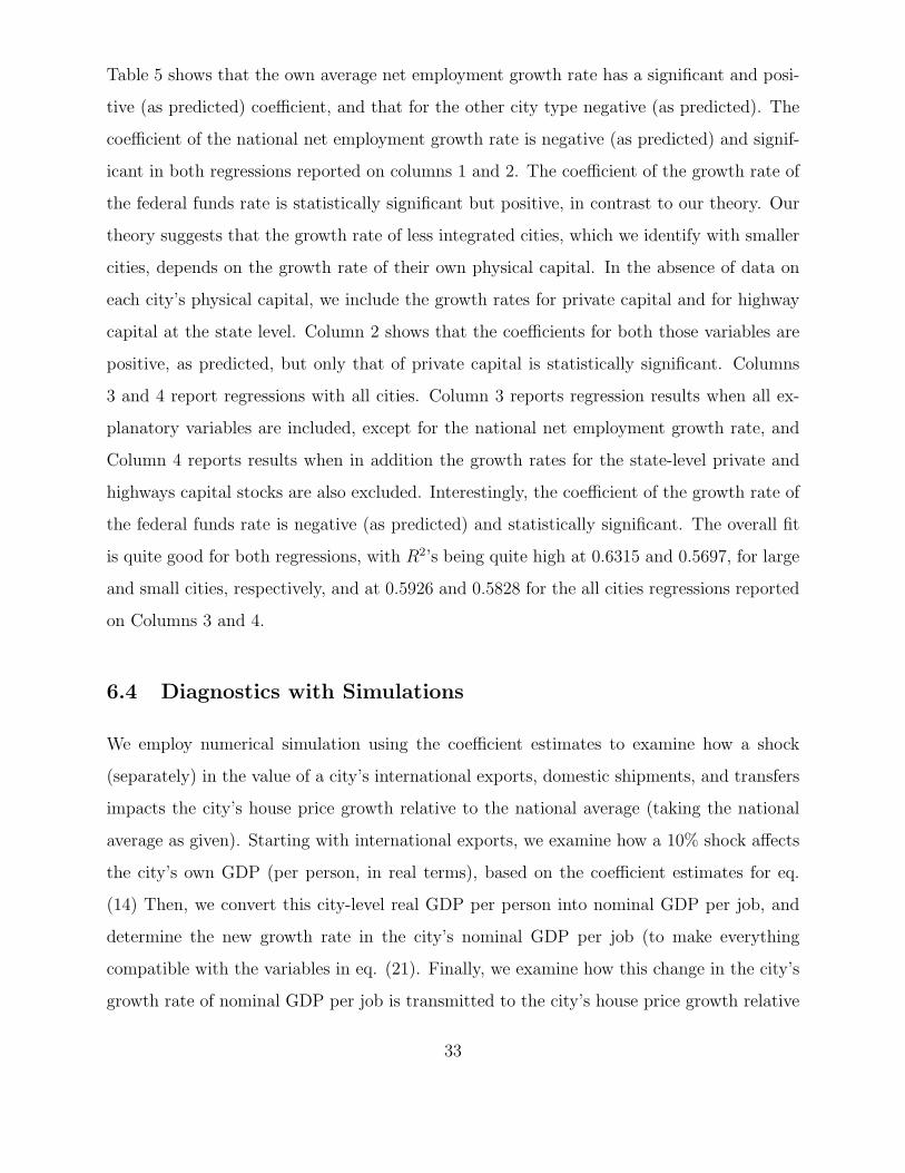
Table 5 shows that the own average net employment growth rate has a significant and posi-

tive (as predicted) coefficient, and that for the other city type negative (as predicted). The

coefficient of the national net employment growth rate is negative (as predicted) and signif-

icant in both regressions reported on columns 1 and 2. The coefficient of the growth rate of

the federal funds rate is statistically significant but positive, in contrast to our theory. Our

theory suggests that the growth rate of less integrated cities, which we identify with smaller

cities, depends on the growth rate of their own physical capital. In the absence of data on

each city’s physical capital, we include the growth rates for private capital and for highway

capital at the state level. Column 2 shows that the coefficients for both those variables are

positive, as predicted, but only that of private capital is statistically significant. Columns

3 and 4 report regressions with all cities. Column 3 reports regression results when all ex-

planatory variables are included, except for the national net employment growth rate, and

Column 4 reports results when in addition the growth rates for the state-level private and

highways capital stocks are also excluded. Interestingly, the coefficient of the growth rate of

the federal funds rate is negative (as predicted) and statistically significant. The overall fit

is quite good for both regressions, with R2’s being quite high at 0.6315 and 0.5697, for large

and small cities, respectively, and at 0.5926 and 0.5828 for the all cities regressions reported

on Columns 3 and 4.

6.4 Diagnostics with Simulations

We employ numerical simulation using the coefficient estimates to examine how a shock

(separately) in the value of a city’s international exports, domestic shipments, and transfers

impacts the city’s house price growth relative to the national average (taking the national

average as given). Starting with international exports, we examine how a 10% shock affects

the city’s own GDP (per person, in real terms), based on the coefficient estimates for eq.

(14) Then, we convert this city-level real GDP per person into nominal GDP per job, and

determine the new growth rate in the city’s nominal GDP per job (to make everything

compatible with the variables in eq. (21). Finally, we examine how this change in the city’s

growth rate of nominal GDP per job is transmitted to the city’s house price growth relative

33

to the national average house price growth. We perform such simulation exercises separately

for a shock to international exports, domestic shipments, and transfers, for a set of 43 cities

for which the city definitions are consistent in both equations (14) and (21). The results,

reported in Figures 1, 2, and 3, for each city show the change in local relative to national

house price growth, based on the fitted value of house price growth in eq. (21) using 2012

actual GDP growth data for the initial point in the graph. The second point in the graph

is the fitted value from (21), using the GDP growth rate based on the shock to GDP in eq.

(14). We also report confidence bands in these graphs (of +/ − 2 standard deviations), as

the dotted lines.

The results imply that a shock to exports leads to an increase in house price growth

relative to the national average in all cities in our sample (except for New Orleans). Also,

the effect of the shock is quite dramatic in most cases. In contrast, a shock to domestic

shipments and to transfers leads to more mixed results: some cities experience flat growth,

others slightly lower growth, and some slightly positive growth. The shock in our simulations

is a one-time, transitory shock. Therefore, residents in some cities may not regard such

a transitory shock as sufficient to lead to a permanent change in their income to warrant

purchasing a house, and therefore there is less impact on housing markets (and price growth).

Perhaps in the case of transfers, residents receive increased unemployment payments when

they lose their primary source of employment income, and for this reason, the results on

the housing market are much more mixed. Thus, it is interesting that a transitory shock to

exports has a relatively large and almost universally positive impact on the housing markets.

In this case, perhaps there is less crowding out of GDP that occurs when exports increase,

relative to an increase in domestic shipments, and therefore this may explain why there is

such a relatively dramatic effect on the housing markets in response to a transitory shock to

exports.

34

7 Conclusions

This is the first paper, to the best of our knowledge, which aims at estimating an equilibrium

urban macro model that links a city’s presence in domestic and international trade to its

growth rate performance. We estimate the GDP determination equation, a spatial equi-

librium equation, and two sets of growth rate regressions. Our primary empirical findings

confirm the comparative statics implications of our theoretical model. In several cases, such

as in the spatial equilibrium equation, we have controlled for endogeneity with an Instru-

mental Variables (IV) approach. One of the unique facets of our work is analogous to Autor,

Dorn and Hanson (2013). They examine how imports from China affect the labor markets in

U.S. ”commuting zones”. Our efforts have the potential to shed some light on transmission

of labor market shocks on goods markets in trading cities. In turn, we then demonstrate

through a parallel empirical analysis that changes to the city-level goods markets affect local

housing prices. In other words, our findings imply that trading cities’ labor market shocks

can indirectly impact the housing markets through the goods markets, and these effects can

vary depending on whether the trading cities are ”large” or ”small”.

It would be interesting to explore the potential of the model to explain housing price

dynamics and economic growth in a number of truly global cities, like New York, San Fran-

cisco, Vancouver, London, Singapore, Hong Kong, etc. In those cities and many others, it

is not only international trade but also foreign investment in housing and real estate that

plays an important but not well understood role. These issues clearly deserve attention in

future research.

35

8 References

Autor, David H., David Dorn, and Gordon H. Hanson. 2013. “The China Syndrome:

Local Labor Market Effects of Import Competition in the United States.” American

Economic Review. 103(3):2121-2168.

Baum-Snow, Nathaniel. 2007. “Did Highways Cause Suburbanization?” Quarterly Journal

of Economics. 122(2):775-805.

Braymen, Charles, Kristie Briggs, and Jessica Boulware. 2011. “R&D and the Export

Decision of New firms.” Southern Economic Journal. 78(1):191–210.

Cardarelli, Roberto, and Lusine Lusinyan. 2015. “U.S. Total Factor Productivity Slow-

down: Evidence from the U.S. States.” IMF working paper WP/15/116. May.

Carruthers, John I., Michael K. Hollar, and Gordon F. Mulligan. 2006. “Growth and

Convergence in the Space Economy: Evidence from the United States. Presented at

the ERSA, Volos, Greece.

Coccia, Mario. 2013. “The Effect of Country Wealth on Incidence of Breast Cancer.”

Breast Cancer Research and Treatment. 141(2):225–229.

Davis, and Michael G. Palumbo. 2008. “The Price of Residential Land in Large U.S. Cities.

Journal of Urban Economics. 63(1):352–384.

Diaz-Lanchas, Jorge, Carlos LLano, Asier Minondo, and Francisco Requena. 2016. “Cities

Export Specialization.” Universitat de Valencia working paper, WPAE-2016-04.

Doherty, Conor. 2017. “Why Falling Home Prices Could Be a Good Thing.” The Upshot.

New York Times. February 10. https://www.nytimes.com/2017/02/10/upshot/popping-

the-housing-bubbles-in-the-american-mind.html

Duranton, Gilles, and and Diego Puga. 2005. “From Sectoral to Functional Urban Special-

ization.” Journal of Urban Economics. 57(2):343–370.

36

Duranton, Gilles, Peter M. Morrow, and Matthew A. Turner. 2014. “Roads and Trade:

Evidence from the US.” Review of Economic Studies. 81(2):681–724.

doi:10.1093/restud/rdt039

Eaton, Jonathan. 1988. “Foreign-Owned Land.” American Economic Review. 78(1):76–88.

Englund, Peter, and Yannis M. Ioannides. 1993. “The Dynamics of Housing Prices: an

International Perspective. 175–197. In Bos, Dieter, ed., Economics in a Changing

World. MacMillan.

Englund, Peter, and Yannis M. Ioannides. 1997. “House Price Dynamics: An International

Empirical Perspective.” Journal of Housing Economics. 6:119–136.

Ferris, Jennifer, and David Riker. 2015. “The Exports of U.S. Cities: Measurement and

Economic Impact.” Office of Economics Working Paper 2015-09B. US International

Trade Commission, Washington, DC.

Fujita, Masahisa, Paul Krugman and Anthony J. Venables. 1999. The Spatial Economy:

Cities, Regions, and International Trade. Cambridge, MA: MIT Press.

Fujita, Masahisa, and Jacques-Francois Thisse. 2009. The Economics of Agglomeration.

Cambridge and New York: Cambridge University Press.

Glaeser, Edward L. and Joseph Gyourko. “The Economic Implications of Housing Supply.

” Journal of Economic Perspectives, forthcoming.

http://realestate.wharton.upenn.edu/research/papers/full/802.pdf

Glaeser, Edward L., Joseph Gyourko, Eduardo Morales, and Charles G. Nathanson. 2014.

“Housing Dynamics: An Urban Approach.” Journal of Urban Economics. 81:45–56.

Grant, William B. 2014. “A Multicountry Ecological Study of Cancer Incidence Rates in

2008 with Respect to Various Risk-Modifying Factors.” Nutrients. 6(1):163-189.

Gruber, Jonathan. 1997. “The Consumption Smoothing Benefits of Unemployment Insur-

ance.” The American Economic Review. 87(1):192-205.

37

Gyourko, Joseph, Christopher Mayer, and Todd Sinai. 2013. “Superstar Cities” American

Economic Journal: Economic Policy. 5(4):167–199.

Henderson, J. Vernon. 1974. “The Sizes and Types of Cities.” American Economic Review.

64:640-656.

Hollar, Michael K. 2011. “Central Cities and Suburbs: Economic Rivals or Allies?” Journal

of Regional Science. 51(2):231–252.

Hornbeck, Richard, and Enrico Moretti. 2015. “Who Benefits From Productivity Growth?

The Local and Aggregate Impacts of Local TFP Shocks on Wages, Rents, and Inequal-

ity.” working paper.

http://faculty.chicagobooth.edu/richard.hornbeck/research/papers/tfp hm may2015.pdf

Hsieh, Chiang-Tai, and Enrico Moretti. 2017. “Housing Constraints and Spatial Misallo-

cation.” May 18. www.nber.org/papers/w21154

Ioannides, Yannis M. 2013. From Neighborhoods to Nations: the Economics of Social In-

teractions. Princeton, NJ: Princeton University Press.

Larson, William D. 2013. “Housing and Labor Market Dynamics in Growing versus De-

clining Cities.” Bureau of Economic Analysis working paper. November.

Lewandowski, James P. 1998. “Economies of Scale and International Exports of SIC 35

from US Metropolitan Areas.” Middle States Geographer. 31:103-11O.

Li, Jinyue. 2017. “Housing Prices and the Comparative Advantage of Cities.” Working

Paper, Chinese University of Hong Kong.

Pennington-Cross, Anthony. 1997. “Measuring External Shocks to the City Economy: An

Index of Export Prices.” Real Estate Economics. 25(1):105–128.

Saiz, Albert. 2010. “The Geographic Determinants of Housing Supply.” Quarterly Journal

of Economics. 1253–1296.

38

United States Bureau of the Census. Annual Survey of Manufactures.

https://www.census.gov/programs-surveys/asm.html

United States Bureau of the Census. State Government Finances.

https://www.census.gov/govs/state/historical data.html

Vachon, Todd E., and Michael Wallace. 2013. “Globalization, Labor Market Transforma-

tion, and Union Decline in U.S. Metropolitan Areas.” Labor Studies Journal. 1–27.

doi: 10.1177/0160449X13511539

Ventura, Jaume. 2005. “A Global View of Economic Growth.” In Handbook of Economic

Growth, eds. Aghion, Philippe, and Steven N. Durlauf, Ch. 22, 1419-1497. Amster-

dam: Elsevier.

39

9 Appendix A (Not for Publication): The Urban Pro-

duction Structure

We develop first the case where all cities are autarkic, that is no intercity trade, and cities

produce both manufactured tradeable goods, and use them in turn to produce the composite

used for consumption and investment. Each of the manufactured tradeable goods, j = X,Y,

is produced by a Cobb-Douglas production function, with constant returns to scale, using

a composite of raw labor and physical capital, with elasticities 1− ϕJ , and ϕJ , respectively,

and a composite made of intermediates. The shares of the two composites are uJ , 1 − uJ

respectively. There exists an industry J−specific total factor productivity, ΞJt. Production

conditions for each of two industries J are specified via their respective total cost functions:

BJt(QJt) =

1

ΞJt

(Wt

1− ϕJ

)1−ϕJ(Rt

ϕJ

)ϕJuJ [∑

m

PZt(m)1−σ

] 1−uJ1−σ

QJt, (31)

where QJt is the total output of good J = X,Y, PZt is the price of the typical intermediate,

elasticity parameters uJ , ϕJ satisfy 0 < uJ , ϕJ < 1, and the elasticity of substitution in the

intermediates composite σ is greater than 1. The TFP term ΞJt, summarizes the effect on

industry productivity of geography, institutions and other factors that are exogenous to the

analysis.

Each of the varieties of intermediates used by industry J are produced according to a

linear production function with fixed costs (which imply increasing returns to scale), with

fixed and variable costs incurred in the same composite of physical capital and raw labor

that is used in the production of manufactured goods X and Y. The shares of the productive

factor inputs used are the same as, ϕJ and 1− ϕJ , J = X,Y, respectively.23 The respective

total cost function is

bit(ZJt(m)) =f + cZJt(m)

ΞJt

( Wt

1− ϕJ

)1−ϕJ(Rt

ϕJ

)ϕJ ,

23This may be generalized to allow for input-output linkages by requiring (see also Fujita, et al. (1999),

Ch. 14), that each intermediate good industry use its own composite as an input. This is accomplished by

introducing as an additional term[∫Mit

0p1−ϵiit

]on the r.h.s. of the cost function bit(ZJt).

40

and ZJt(m), the quantity of the input variety m used by industry J = X,Y. Its price is

determined in the usual way from the monopolistic price setting problem [Dixit and Stiglitz

(1977)] and it is equal to marginal cost, marked up by σσ−1

:

PZ,J,t =σ

σ − 1

c

ΞJt

(Wt

1− ϕJ

)1−ϕJ(Rt

ϕJ

)ϕJ

.

At the monopolistically competitive equilibrium with free entry, each of the intermediates

is supplied at quantity (σ − 1)fc, and costs σf

ΞJt

(Wt

1−ϕJ

)1−ϕJ(Rt

ϕJ

)ϕJper unit to produce. Its

producer earns zero profits.

10 Appendix B (Not for Publication): Derivations of

City GDP for the Urban System with International

Trade

We proceed to modify the model of the urban system by postulating that while cities spe-

cialize, some of the cities export to, while other import from, the international economy. We

modify the urban structure as follows. There are nX cities that specialize in the production

of good X and sell all of their output within the domestic economy producing QX each;

there are nX,x cities each with population NX,x also specializing in the production of good X

that in addition export QX,ex of their output, producing in total QX,p each. Similarly, there

are nY cities that specialize in the production of good Y and sell all of their output QY in

the domestic economy; and there are nY,m cities each with population NY,m specializing in

the production of good Y , producing Y in quantity QY,p each, which also import QY,im. We

simplify the derivations by assuming that the quantities of imports and exports are given.

The national population is distributed over all cities, as before:

nXNX + nX,xNX,x + nYNY + nY,mNY,m = N. (32)

Similarly, total capital is allocated to all cities:

nXKX + nX,xKX,x + nYKY + nY,mKY,m = K. (33)

41

International trade balance requires that the value of the national exports of good X equal

the value of the national imports of good Y :

nX,xPXQX,ex = nY,mPYQY,im. (34)

Domestic trade balance requires that spending by all X cities on good Y equal spending on

good X by all Y cities:

(1− α)nXPXQX + (1− α)nX,xPXQX,p = αnYNY PX + αnY,mNY,mQY,p. (35)

These conditions along with the conditions for spatial equilibrium and capital market equi-

librium across cities of all types allows us to solve for capital allocation and thus for the

output by different types of cities, given city populations and numbers by type. A tedious

set of derivations (see Appendix) yields the capital allocations to different city types, as

fractions of the aggregate capital, with the factors of proportionality being functions of city

sizes and numbers and of parameters.

Thus, using the expressions from the Appendix in (44) we obtain expressions for output

for each city type X,Y . The counterparts for city types X, x and Y,m, respectively those

that export good X and import good Y, are:

QX,x = ΞX,xHµX(1−ϕX)X,x KµXϕX

X,x , QY,m = ΞY,mHµY (1−ϕY )Y,m KµY ϕY

Y,m , (36)

. The corresponding growth rates for city output of each type are obtained by taking logs

and first-differencing. That is,

GR(QX,x,t) = GR(ΞX,t) + µXϕX [GR(FPKX,t) + GR(Kt)] + µX(1− ϕX)GR(HX,x,t), (37)

where GR(FPKX,t) denotes the factor of proportionality in the expression for KX,t, and

Hc,X,x,t is given by (4), forNX,x(t). An expression similar to (37 ) is obtained for GR(QY,m,t) =

lnQY,m,t+1 − lnQY,m,t.

This model is formulated in terms of two different tradeable goods, which are traded

domestically and internationally and are used in each city to produce a non-tradeable good

that is used for consumption and investment. The model may be generalized, following

42

Ventura (2005) to the case of many goods. The simplified two-good case makes it clear

that the output growth rates for different city types are described by structurally different

expressions, that is for autarkic cities, for cities that trade domestically and for cities that

export or import internationally.

For the cities that neither export nor import internationally, conditions (9.29–9.31) in

Ioannides, op. cit., that follow from the assumptions of capital mobility and spatial equilib-

rium continue to hold. In addition, the counterpart of (9.29) for cities of type X and Xex

yields the counterpart of (9.30), which is implied by spatial equilibrium:

PXQX

PXQX,p

=NX

NX,x

. (38)

And similarly for cities of type Y and Yim :

PYQY

PYQY,p

=NY

NY,m

. (39)

In other words, the relative share of output by cities of type X,Y are proportional to their

respective relative populations. Free capital mobility between X,Y cities implies condition

(9.31) in Ioannides, op. cit.,KX

KY

=NX

NY

ϕX(1− ϕY )

ϕY (1− ϕX), (40)

and between X-type cities and X type exporting cities

KX,x

KX

=NX,x

NX

, (41)

and between Y -type cities and Y type importing cities

KY,m

KY

=NY,m

NY

. (42)

These intermediate results will be critical in our derivation of expressions for city output in

the presence of international trade.

In each city output of the composite good, which is not traded but is used for consumption

and investment is produced by using quantities of tradeable goods X,Y according to

QX = QαXQ

1−αY .

43

The corresponding (natural) price index is:

P ≡(PX

α

)α ( PY

1− α

)1−α

,

which can be normalized and set equal to 1.

The objective of the analysis is to write expressions for real output of different city types,

given total capital and total labor in the economy, (K,N), and given the sizes of different

city types, (NX , NX,x, NY , NY,m). For example, the real income of a city of type X is PXQX ,

which by using the normalization condition and the spatial equilibrium condition may be

written as

αα(1− α)1−αQαXQ

1−αY

(NX

NY

)1−α

, (43)

where:

QX = ΞXHµX(1−ϕX)X KµXϕX

X , QY = ΞYHµY (1−ϕY )Y KµY ϕY

Y , (44)

where µX , µY may actually be greater or less than 1. The counterparts of these expressions

follow for the other types of cities.

We proceed by using the spatial equilibrium conditions among cities of type X,Y , (38)

and (39), in the domestic trade balance condition (35) to eliminate QX,p, QY,p. We thus have:

(1− α)[nX +

NX,x

NX

]PXQX = α

[nY + nY,m

NY,m

NY

]PYQY .

Solving for PXQX

PY QYgives:

PXQX

PYQY

=α

1− α

NX

NY

nYNY + nY,mNY,m

nXNX + nX,xNX,x

. (45)

This is a straightforward generalization of the condition in the absence of international trade:

if nX,x = nY,m = 0, the spending on good Y by each city of type X is equal to the spending

on good X by each city of type Y . From the ratio of the value of output of the typical

exporting to importing city follows:

PXQX,p

PYQY,m

=α

1− α

NX,x

NY,m

nYNY + nY,mNY,m

nXNX + nX,xNX,x

. (46)

Rearranging the international trade balance condition (34) gives an equation for the

terms of trade:PX

PY

=nY,m

nX,x

QY,im

QX,ex

. (47)

44

Rewriting the labor market condition by using the spatial equilibrium conditions yields:

nXNX + nX,xNXPXQX,p

PXQX

+ nYNY + nY,mNYPYQY,p

PYQY

= N.

Using it along with the domestic trade balance condition as a simultaneous system of equation

allows us to solve for (nX,xPXQX,p, nY,mPYQY,p) and obtain:

nX,xPXQX,p =α(N − nXNX)− (1− α)nXNY

PXQX

PY QY

(1− α) NY

PY QY+ α NX

PXQX

; (48)

nY,mPYQY,p =(1− α)(N − nYNY )− αnYNX

PY QY

PXQX

(1− α) NY

PY QY+ α NX

PXQX

; (49)

Dividing Eq. (49) by Eq. (48) and rearranging allows us to expressnY,m

nX,xin terms of PXQX

PY QY.

Then, using Eq. (47) yields an expression for the terms of trade, in terms ofQY,im

QX,ex, which

are given, (nX , NX ;nX,x, NX,x;nY , NY ;nY,mNY,m), and parameters:

PX

PY

=QY,im

QX,ex

NX,x

NY,m

(N − nYNY )(nYNY + nY,mNY,m)− nYNY (nXNX + nX,xNX,x)

(N − nXNX)(nXNX + nX,xNX,x)− nXNX(nYNY + nY,mNY,m). (50)

This solution demonstrates an important role for international trade on the urban structure.

It is simplified by solving next below for nXNX + nX,xNX,x, nYNY + nY,mNY,m. The expres-

sions obtained for outputs by different types of cities, namely exporting and non-exporting

cities of different types differ depending upon each city type.

Working with the capital mobility conditions (40), (41), and (42) allows us to solving for

the capital allocations to different city types and therefore write expressions for real output,

the counterparts of (43) for city types that export X and that import Y . This yields:

nXNX+nX,xNX,x =α(1− ϕX)

α(1− ϕX) + (1− α)(1− ϕY )N ;nYNY+nY,mNY,m =

(1− α)(1− ϕY )

α(1− ϕX) + (1− α)(1− ϕY )N.

(51)

This solution in turn simplifies (50). It also simplifies (45), which becomes:

PXQX

PYQY

=1− ϕY

1− ϕX

NX

NY

,

and (46), which becomes:PXQX,p

PYQY,m

=1− ϕY

1− ϕX

NX,x

NY,m

.

45

The allocations of total capital to the different types of cities are:

KX =NXϕX(1− ϕY )

nXNXϕX(1− ϕY ) + nX,xNX,xϕX(1− ϕY ) + nYNY ϕY (1− ϕX) + nY,mNY,mϕY (1− ϕX)K

KX,x =NX,xϕX(1− ϕY )

nXNXϕX(1− ϕY ) + nX,xNX,xϕX(1− ϕY ) + nYNY ϕY (1− ϕX) + nY,mNY,mϕY (1− ϕX)K

KY =NY ϕY (1− ϕX)ϕX(1− ϕY )

nXNXϕX(1− ϕY ) + nX,xNX,xϕX(1− ϕY ) + nYNY ϕY (1− ϕX) + nY,mNY,mϕY (1− ϕX)K

KY,m =NY,mϕY (1− ϕX)

nXNXϕX(1− ϕY ) + nX,xNX,xϕX(1− ϕY ) + nYNY ϕY (1− ϕX) + nY,mNY,mϕY (1− ϕX)K

46

11 Tables

• Table 1a, 1b, 1c, 1d, 1e: Descriptive Statistics

• Table 2: Estimation Results for City GDP determination, Eq. (14), for 76 cities, 2002,

2007, 2012

• Table 3: Estimation Results for Spatial Equilibrium, Eq. (15), 26 MSA’s, 2003-2012

• Table 4: Estimation Results for Eq. (21), 96 MSA’s, 2003–2012

• Table 5: Growth Regressions for Large and Small Cities, Equations (28), (29).

47

48

49

50

\\Table1b

:Descriptive

Statistics

forVariables

inEq

uation

13,26MSA

's,200

220

12

grow

thinland

valuepe

rjobMSA

grow

thinland

perjobtotalgrowth

inGDPpe

rjobMSA

grow

thinGDPpe

rjobtotgrow

thinCP

IMSA

grow

thinCP

I"allurban

"

Mean

0.03

4436

270.00

6164

210.03

7821

680.03

7204

510.02

3635

650.02

3941

09

Med

ian

0.02

5989

660.00

9934

210.03

7133

190.03

6442

390.02

5647

880.02

6630

43

Max

1.55

7959

0.13

8860

10.11

6327

20.05

7829

280.05

1872

150.03

8395

5

Min

0.85

1878

10.20

5807

0.07

5489

920.02

0668

360.02

6436

880.00

3557

78

Std.Dev.

0.26

9325

10.12

1461

30.01

9292

850.01

3520

30.01

3013

730.01

1113

51

Obs

286

260

286

260

286

286

51

52

Table1c:DescriptiveStatisticsforVariablesinEquation20,96MSA's,20032012

Growth

inCPI(region)

Growth

inCPI(M

SA)

Growth

inGDPperjob(M

SA)Growth

inGDPperjob(nation)

Jobspercapita(nation)

Jobspercapita(M

SA)

Mean

0.025275982

0.024520681

0.03566983

0.03622301

0.441852852

0.437501623

Median

0.026948288

0.028339157

0.034661982

0.039357728

0.451738849

0.44866066

Max

0.046546547

0.03785489

0.219547493

0.051632747

0.459386936

0.607012932

Min

0.004350979

0.001119453

0.07355889

0.020502477

0.41812985

0.00000000

Std.Dev.

0.011374057

0.011605292

0.024786624

0.011531386

0.016355196

0.075315113

Obs

970

970

960

970

970

970

Growth

inCancerdeathsperjob(M

SA)Growth

inCancerdeathsperjob(NATION)Unavailablelandshare

(MSA)

House

priceelasticity

WhartonLandUse

RegulationIndex

Mean

0.00430883

0.001036258

0.261474748

1.897750344

0.073577796

Median

0.000415332

0.008334288

0.192263633

1.668164492

0.034924999

Max

0.205606671

0.055564962

0.796446204

5.453317165

1.892059565

Min

0.136303455

0.018477636

0.009316998

0.595266104

1.23920691

Std.Dev.

0.04312148

0.021239225

0.2091283

0.9204122

0.668382832

0.767233036

0.893310739

Obs

960

970

970

970

970

53

Table1d

:Descriptiv

eStatisticsforV

ariables

inEq

uatio

n27

,180

MSA

's,200

620

10

Nom

inalGDP($million)

LargeCitie

sEffectiveJobs

(net

ofcommutetim

e)Sm

allCities

EffectiveJobs

(net

ofcommutetim

e)

Mean

66610.098266

537051

60962

Median

23986

228475

62120

Max

1280307

7584130

62961

Min

9637

47593

57844

Std.Dev.

130187.848132

865517

2025

Obs

865

865

865

"Nationa

l"Average

EffectiveJobs,n

etof

commutetim

eStatelevelTFP

Growth

Fede

ralFun

dsRa

te(Nationa

l)

Mean

294202

0.001368826

2.71

Median

298095

0.00264581

3.94

Max

301586

0.07566632

5.25

Min

284771

0.07467376

0.11

Std.Dev.

7150

0.025750115

2.19

Obs

865

855

865

54

55

56

57

Tabl

e 2:

Est

imat

ion

Res

ults

for

Equa

tion

14,

for

76 "

Citi

es",

Ann

ual "

City

-leve

l" D

ata

for

2002

, 200

7, 2

012

Dep

ende

nt V

aria

ble:

REA

L G

DP

PER

PERS

ON

Inde

pend

ent V

aria

bles

OLS

RE

FEO

LSR

EFE

IVIV

-RE

IV-F

EIV

IV-R

EIV

-FE

CON

STA

NT

3844

8.01

6**

**39

229.

077

****

4050

7.85

5**

**35

050.

090

****

3701

2.72

6**

**40

659.

348

****

3604

3.07

9**

**36

158.

051

****

3191

4.42

5**

**33

552.

293

****

3463

1.61

1**

**34

281.

568

****

2757

.168

3187

.896

2707

.424

1304

.043

698.

786

1669

.969

5117

.979

3537

.017

1289

.395

5556

.979

4829

.914

2587

.825

DO

MES

TIC

SALE

S PE

R JO

B0.

045

**0.

056

**0.

039

0.

150

***

0.12

3**

0.03

9

0.12

0

0.14

3

0.38

3**

**0.

220

0.

217

0.

293

****

0.02

00.

028

0.06

20.

045

0.04

90.

037

0.23

60.

144

0.04

10.

280

0.18

90.

076

TRA

NSF

ERS

PER

JOB

1.09

8tt

1.04

9tt

tt1.

054

tttt

--

-0.

200

t0.

139

t0.

248

t-

--

0.04

80.

062

0.06

1-

--

0.24

80.

260

0.26

6-

--

EXPO

RTS

PER

JOB

0.62

2tt

tt0.

348

t0.

155

1.

393

tttt

1.01

0tt

tt0.

660

ttt

1.26

6tt

tt1.

096

tttt

0.61

2

1.35

6tt

tt1.

063

tttt

0.69

8tt

t

0.47

70.

239

0.09

00.

586

0.32

80.

192

0.73

50.

558

0.09

90.

664

0.37

00.

175

N16

616

616

616

616

616

616

016

016

016

116

116

1

R-sq

uare

d0.

598

0.55

90.

910

0.26

10.

186

0.82

20.

376

0.31

20.

805

0.25

90.

192

0.79

2

J-st

atis

tic

(P-V

alue

)-

--

--

-0.

074

0.39

20.

599

0.20

80.

563

0.72

6

Not

es:

Whi

te R

obus

t sta

ndar

d er

rors

in b

old

FE is

"cr

oss-

sect

iona

l fix

ed e

ffec

ts"

RE is

"cr

oss-

sect

iona

l ran

dom

eff

ects

"

IV is

"In

stru

men

tal V

aria

bles

"

Sam

ple

size

s ar

e le

ss th

an 2

28 (7

6 ci

ties

for 3

yea

rs) d

ue to

mis

sing

val

ues

for s

ome

regr

esso

rs a

nd/o

r ins

trum

ents

all v

aria

bles

are

in "

real

" te

rms,

200

5 do

llars

****

, ***

, **,

* in

dica

tes

the

coef

ficie

nt is

sta

tistic

ally

sig

nific

antly

diff

eren

t fro

m 0

at t

he 0

.001

, 0.0

1, 0

.05,

0.1

0 le

vels

, res

pect

ivel

ytt

tt, t

tt, t

t, t in

dica

tes

the

coef

ficie

nt is

not

sta

tistic

ally

sig

nific

antly

diff

eren

t fro

m 1

at t

he 0

.10,

0.0

5, 0

.01,

0.0

01 le

vels

, res

pect

ivel

y (a

larg

er n

umbe

r of s

ymbo

ls in

dica

tes

grea

ter d

egre

e of

con

fiden

ce th

at th

e co

effic

ient

equ

als

1)

Inst

rum

ents

incl

ude:

for

dom

estic

shi

pmen

ts:

lagg

ed "

plan

ned

high

way

rays

" pe

r-ca

pita

, lag

ged

mile

s of

hig

hway

s co

mpl

eted

(ins

ide

the

city

), an

d th

e di

ffer

ence

bet

wee

n na

tiona

l pop

ulat

ion

and

city

pop

ulat

ion;

for

tran

sfer

s: re

al u

nem

ploy

men

t ins

uran

ce re

ceip

ts p

er p

erso

n

for e

xpor

ts (r

eal e

xpor

ts p

er p

erso

n) is

the

inst

rum

ent f

or it

self

(sin

ce d

eman

d fo

r exp

orts

ass

umed

exo

geno

us to

a c

ity)

for c

onst

ant t

erm

(whe

re a

pplic

able

) is

the

inst

rum

ent f

or it

self;

58

59

Table 3: Estimation Results for Equation 13, 26 MSA's, 2003 2012

Dependent Variable: LAND RENT GROWTH RATE PER JOB DIFFERENCE GDP GROWTH RATE PER JOB DIFFERENCE

P Value in bold

Independent Variables OLS Fixed Effects

CONSTANT 3.984608 1.043285

0.0050 0.8872

MSA CPI GROWTH URBAN CPI GROWTH 5.644318 6.299464

0.0006 0.0001

N 260 260

R squared 0.044416 0.364512

60

Table 4: Estimation Results for Equation 20, 96 MSA's, Annual Data, 2003-2012

Spatial Equilibrium Equation

Dependent Variable: MSA House Price Growth Rate - National House Price Growth Rate

P-Values in bold

OLS IV

Independent Variables

Constant -1.9343 -1.0584

0.3419 0.7706

REGIONAL CPI Growth - Urban CPI Growth -0.2893 -1.3505

0.4126 0.1024

MSA GDP growth per capita - National GDP Growth per capita 0.2943 4.2281

0.0009 0.0347

(MSA Employment per-capita)1/2

-0.0076 0.0411

0.1121 0.5035

(-1)×(National Employment per-capita)1/2

0.2816 0.2032

0.3519 0.7062

N 960 960

R-squared 0.0368 *

J-Statistic - 0.1217

Note: All models include region and year fixed effects

Instruments for IV Estimation:

Unavailable Land Area;

Wharton Regulation Index;

House Price Elasticity;

MSA Cancer Growth - National Cancer Growth

*R-squared from IV may be negative, in which situation it is not useful to report (Wooldridge, 2006)

61

62

-.6

-.4

-.2

.0

.2

.4

.6

Alb

any,

NY

Atla

nta

Aus

tin, T

X B

altim

ore

Birm

ingh

am, A

L B

osto

n B

uffa

lo

Cha

rlotte

, NC

C

hica

go

Cin

cinn

ati

Cle

vela

nd

Col

umbu

s, O

H

Day

ton,

OH

D

enve

r D

etro

it G

rand

Rap

ids,

MI

Gre

ensb

oro,

NC

G

reen

ville

, SC

H

oust

on

Indi

anap

olis

J

acks

onvi

lle, F

L L

as V

egas

L

os A

ngel

es

Lou

isvi

lle, K

Y M

emph

is, T

N

Milw

auke

e M

inne

apol

is

Nas

hville

, TN

N

ew O

rlean

s, L

A V

irgin

ia B

each

, VA

Sal

t Lak

e C

ity

Okl

ahom

a C

ity

Orla

ndo,

FL

Phi

lade

lphi

a P

hoen

ix

Pitt

sbur

gh

Por

tland

, OR

R

ichm

ond,

VA

Roc

hest

er, N

Y S

an A

nton

io, T

X S

an D

iego

S

eattl

e T

ampa

DEP_VBLE_EXPORTS_SHOCK – 2 S.E.

Gro

wth

Rat

e in

City

Hou

sing

Pric

esRe

lativ

e to

Nat

iona

l Ave

rage

Simulations of a 10% Shock in Value of a City’s International Exportson the City’s Growth in Housing Prices Relative to National Average

-.6

-.4

-.2

.0

.2

.4

.6

Alb

any,

NY

Atla

nta

Aus

tin, T

X B

altim

ore

Birm

ingh

am, A

L B

osto

n B

uffa

lo

Cha

rlotte

, NC

C

hica

go

Cin

cinn

ati

Cle

vela

nd

Col

umbu

s, O

H

Day

ton,

OH

D

enve

r D

etro

it G

rand

Rap

ids,

MI

Gre

ensb

oro,

NC

G

reen

ville

, SC

H

oust

on

Indi

anap

olis

Ja

ckso

nville

, FL

Las

Vega

s L

os A

ngel

es

Lou

isvi

lle, K

Y M

emph

is, T

N

Milw

auke

e M

inne

apol

is

Nas

hville

, TN

N

ew O

rlean

s V

irgin

ia B

each

, VA

Sal

t Lak

e C

ity

Okl

ahom

a C

ity

Orla

ndo,

FL

Phi

lade

lphi

a P

hoen

ix

Pitt

sbur

gh

Por

tland

, OR

R

ichm

ond,

VA

Roc

hest

er, N

Y S

an A

nton

io

San

Die

go

Sea

ttle

Tam

pa

DEP_VBLE_SHIPMENTS_SHOCK– 2 S.E.

Gro

wth

Rat

e in

City

Hou

sing

Pric

es

Rel

ativ

e to

Nat

iona

l Ave

rage

Simulations of a 10% Shock in Value of a City’s Domestic Shipmentson the City’s Growth in Housing Prices Relative to National Average

-.6

-.4

-.2

.0

.2

.4

.6 A

lban

y, N

Y A

tlant

a A

ustin

, TX

Bal

timor

e B

irmin

gham

, AL

Bos

ton

Buf

falo

C

harlo

tte, N

C

Chi

cago

C

inci

nnat

i C

leve

land

C

olum

bus,

OH

D

ayto

n, O

H

Den

ver

Det

roit

Gra

nd R

apid

s, M

I G

reen

sbor

o, N

C

Gre

envi

lle, S

C

Hou

ston

In

dian

apol

is

Jac

kson

ville

, FL

Las

Veg

as

Los

Ang

eles

L

ouis

ville

, KY

Mem

phis

, TN

M

ilwau

kee

Min

neap

olis

N

ashv

ille, T

N

New

Orle

ans

Virg

inia

Bea

ch, V

A S

alt L

ake

City

O

klah

oma

City

O

rland

o, F

L P

hila

delp

hia

Pho

enix

P

ittsb

urgh

P

ortla

nd, O

R

Ric

hmon

d, V

A R

oche

ster

, NY

San

Ant

onio

S

an D

iego

S

eattl

e T

ampa

DEP_VBLE_TRANSFERS_SHOCK– 2 S.E.

Gro

wth

Rat

e in

City

Hou

sing

Pric

es

Rel

ativ

e to

Nat

iona

l Ave

rage

Simulations of a 10% Shock in Value of Transfers on the City’s Growth in Housing Prices Relative to National Average