Embed Size (px)
Citation preview

I N T E R N A L L A B O U R M A R K E T M O B I L I T Y I N 2 0 0 5 – 2 0 1 1 : T H E C A S E O F L A T V I A
CONTENTS
ABSTRACT 2
INTRODUCTION 3
1. DATA AND LABOUR FLOW CONSTRUCTING METHODOLOGY 5
2. LABOUR FLOW ANALYSIS 8 2.1 Hiring and separation rates 8 2.2 International comparison 11 2.3 Detailed labour flow analysis 15
3. SURVIVAL ANALYSIS FOR LABOUR MARKET SPELLS 23 3.1 Kaplan–Meier survival estimates 23 3.2 Cox proportional hazards (PH) model 26
3.2.1 Determinants of employment to unemployment movement 27 3.2.2 Determinants of unemployment to employment movement 29
CONCLUSIONS 32
APPENDICES 34
BIBLIOGRAPHY 43
ABBREVIATIONS AT Austria CI confidence interval CSB Central Statistical Bureau of Latvia CY Cyprus EA euro area ECB European Central Bank EE Estonia ES Spain EU European Union FI Finland FR France
GDP gross domestic product GR Greece IE Ireland IT Italy LFS labour force survey MT Malta NL Netherlands PH proportional hazards SI Slovenia SK Slovakia UK United Kingdom
1
I N T E R N A L L A B O U R M A R K E T M O B I L I T Y I N 2 0 0 5 – 2 0 1 1 : T H E C A S E O F L A T V I A
ABSTRACT
This research gives an overview of labour market internal and occupational mobility in Latvia comparing periods before, during and after the crisis. It uses both the labour flow analysis and the survival analysis to evaluate labour mobility and to determine factors influencing it. The analysis is based on labour force survey (LFS) longitudinal data for 2005–2011.
The paper investigates possible asymmetric responses of the labour market during the extreme period of economic boom and bust, provides detailed information on the aspects of labour market mobility (e.g. changes in the types of labour contract, sector and region of work) and factors determining changes in the status of economic activity (employed or unemployed). We also propose a new way for calculating labour market flows to provide information on quarterly changes.
Keywords: Labour mobility, occupational mobility, labour flows, unemployment, labour force survey
JEL classification codes: J23, J61, J62, J64
The views expressed in this publication are those of the authors, employees of the Monetary Policy Department of Latvijas Banka. The authors assume responsibility for any errors and omission. The authors would like to thank Zaiga Priede and Zane Mangale (CSB), Jaanika Meriküll (Bank of Estonia), Oļegs Krasnopjorovs, Mārtiņš Bitāns and Konstantīns Beņkovskis (Bank of Latvia) for their valuable comments and recommendations.
2
I N T E R N A L L A B O U R M A R K E T M O B I L I T Y I N 2 0 0 5 – 2 0 1 1 : T H E C A S E O F L A T V I A
INTRODUCTION
This research explores internal and occupational labour market mobility in Latvia, comparing the situation before, during and after the economic crisis. It combines the labour flow analysis and the survival analysis to give an in-depth overview on determinants and changes in labour mobility in Latvia in different time periods.
Mobility of labour (both internal and external) helps retrieve equilibrium in the economy without introducing changes in wages. The previous research about labour market elasticity in Latvia (Zasova and Meļihovs (2005)) concludes that the institutional environment in Latvia does not impose any significant burden for absorbing different economic shocks through the labour market and, in general, the labour market elasticity in Latvia is higher than in other EU151 Member States. Hazans (2007) has explored this topic on the basis of labour force survey (LFS) data of 2002–2005, suggesting that during this period labour market flexibility in Latvia had improved significantly due to both the increase in external mobility (after joining the EU) and the economic growth contributing to labour market changes.
There are research papers which specifically focus on external labour mobility within the EU after the latter's enlargement, e.g. by Fic et al. (2011), and Ester and Fouarge (2007). Paci et al. (2010) explore internal labour mobility in Central Europe and in the Baltic States using the labour force survey data for 2004. Geographical labour force mobility in Latvia has been investigated by the Ministry of Welfare of the Republic of Latvia (2007a) focusing both on external and internal migration. The emigration problem has likewise been studied in great detail by Hazans and Philips (2011) and Hazans (2007).
In this paper, however, we will focus on internal and occupational mobility of labour, i.e. changes affecting different labour force states (employed, unemployed or economically inactive), types of job contracts, sectors and regions in Latvia. Janiak and Wasmer (2008) underline that occupational and sectoral mobility could be a good substitute for geographical mobility (between countries or regions), because the factors leading to low geographical mobility are likely to impose constraints on occupational mobility. Therefore, the purpose of this research is to look in more detail at labour force internal mobility and the factors determining probability of losing or finding job in Latvia in 2005–2011 by analysing micro data provided in the LFS database.
Labour market research has, since the late 1980s, increasingly focused on dynamic as opposed to stock characteristics of the labour market (Artola and Bell (1999)). There is a relatively long tradition of the labour market flow research (e.g. Pissarides et al. (1986), Blanchard and Diamond (1992), Davis and Haltiwanger (1999)). An ideal data source for this type of research would be a special database on labour market flows, for example, experimental statistics on labour market flows developed by the UK Office for National Statistics based on work by Jenkins and Chandler (2010). Since such databases are not always available, researches use stock data
1 Austria, Belgium, Denmark, Finland, France, Germany, Greece, Ireland, Italy, Luxembourg, the Netherlands, Portugal, Spain, Sweden and the UK.
3
I N T E R N A L L A B O U R M A R K E T M O B I L I T Y I N 2 0 0 5 – 2 0 1 1 : T H E C A S E O F L A T V I A
from LFS as the source of information on household members' economic activity. For example, recent analyses for European countries using LFS data are by the ECB (2012), Meriküll (2011) for Estonia, and Casado et al. (2012) for 11 EU countries. There are also examples of labour mobility research done using other data sources, e.g. administrative data on individual worker and employer histories maintained by unemployment insurance systems as used by Davis and Haltiwanger (1998) in the analysis of the US labour and job flows, and an attempt to use longitudinal monthly data of the EU-SILC database for comparative labour flow analysis in Central Europe as presented by Flek and Mysíková (2012).
The analysis of determinants of individual labour market transitions from/to employment, unemployment or inactivity is often carried out by means of survival analysis or logistic panel regression. Meriküll (2011) investigated how the duration of unemployment and employment spells depends on personal characteristics in Estonia applying a semi-parametric Cox proportional hazards (PH) model. Kuhlenkasper and Steinhardt (2011) applied a dynamic hazard model in their research of the factors influencing the duration of unemployment in Germany. In the case of Latvia, using LFS data for 2002, Hazans (2005) studied the main factors associated with the transition from jobs to unemployment and nonparticipation by applying a multinomial logistic regression model.
This paper studies labour market mobility in Latvia in 2005–2011. We construct quarterly labour flow series and apply the survival analysis to monthly data to study the probability of employment and unemployment status change. This paper contributes to the literature by investigating possible asymmetric responses of the labour market during the extreme period of economic growth and contraction by providing more information on labour market mobility in small open economies with flexible wages. We also propose a new way of labour market flow calculations, which provides information on quarterly changes.
The paper is organised as follows. Section 1 guides through the theoretical aspects of LFS use in the analysis of labour market flows and provides the description of the proposed labour flow analysis approach. Section 2 presents the results of labour flow analysis. Section 3 gives an overview of the results of the survival analysis and Cox PH models,while the final section concludes.
4
I N T E R N A L L A B O U R M A R K E T M O B I L I T Y I N 2 0 0 5 – 2 0 1 1 : T H E C A S E O F L A T V I A
1. DATA AND LABOUR FLOW CONSTRUCTING METHODOLOGY
LFS data in Latvia are collected by the CSB. Similarly as in other European countries, the rotating panel method is used. Data cover the period from 2005 to 2011 and are collected at the household level for people in the age group from 15 to 74. Prior to 2007, this group includes around 10 thousand households per year, but since 2007 the number has risen to around 24 thousand households. During 2005–2006, households were interviewed three times, with a 26 week interval. From 2007, there are four interviews with the intervals of 13, 39 and 13 weeks respectively. Quarterly and yearly weights are provided for each observation, allowing for aggregating the estimated statistics and extrapolating the result for the whole population.
The usual first step to obtain labour flow data from LFS is the construction of longitudinal data by matching records of economic activity (e.g. employed, unemployed or inactive) for the same individual across a number of consecutive interviews. Usually an LFS contains two blocks of questions, i.e. about the current period and those providing retrospective information. Retrospective information tends to be concentrated in two distinct types of questions: those relating to the duration of employment or unemployment and those referring to an individual's labour market status one year ago. The most widespread approach to calculate labour market flows is to compare the current economic activity status (estimated by the interviewer) with retrospective information about the status one year ago (provided by the interviewee), thus obtaining labour flow data over a 12-month period (see, e.g. Elsby et al. (2011), Meriküll (2011) and Hazans (2005)).
There are several potential pitfalls with this approach, as was discussed in detail by Artola and Bell (1999). One of the most important problems is the inconsistency of classification of economical status of household members. For example, the labour market status is typically self-reported by individuals in the retrospective part of questionnaire; the current labour market status, on the other hand, is assigned by the interviewer on the basis of the interviewee's responses to a series of questions regarding his/her labour market activity in the current period. As was shown in Artola and Bell (1999), since the retrospective part of questions contains no information with respect to the job search activity (both its quality and extent), it is very hard to evaluate the correctness of self-evaluation, and, therefore, the estimated flow data are most probably biased.
Another disadvantage of yearly labour market flows is a long (12-month) gap between observations. By construction, changes in the economic activity of interviewee that happened within one year are excluded from the analysis. Therefore, the duration and frequency of flow changes can be undervalued. Also, for policy measure or economic shock transmission evaluation, it is preferable to use short-term labour flow changes in order to assess the immediate effect on the labour market. Taking into account the problems above, we propose a slightly different method for worker flow calculation based on quarterly probability of status change.
The assumption behind the proposed method is that only labour market statuses assigned by the interviewer are used. Thus, labour flows are calculated from the panel data, which include only economic activity statuses for the dates of interview
5
I N T E R N A L L A B O U R M A R K E T M O B I L I T Y I N 2 0 0 5 – 2 0 1 1 : T H E C A S E O F L A T V I A
(where they are automatically assigned on the basis of a set of questions and, therefore, are more plausible). Another assumption refers to assigning equal probability of status change for quarters between observations, since we do not know exactly when the change happened. So, for example, if it is known for a person that there is an observation of employment (Et)2 and that of unemployment (Ut + 2) after 2 quarters, we assign the probability of flow from employment to unemployment (E-to-U) for periods t + 1 and t + 2 to be equal 1/(N – 1) = ½ = 0.5, where N is the number of quarters in the analysed flow interval.
One can argue that high level uncertainty is introduced in such flow estimations, since it is possible to calculate the exact date of the status change from the retrospective question about the duration of present employment or unemployment. As argued in Artola and Bell (1999), the questionnaire is usually filled in by a household member, who might not remember the precise dates of employment/ unemployment termination by other household members. Therefore, the probability of bias and flow overlapping in LFS data is very high. But if we are interested not only in the flows to/from unemployment or employment (E-to-U, U-to-E, I-to-E, E-to-I) but also in the flows between unemployment and inactivity (U-to-I, I-to-U), which are very important when evaluating the effectiveness in people's return to economic activity, there are no retrospective questions that would help us detect the date precisely. Therefore, in order to be consistent, all flow statistics are estimated using probabilities of status change between the interview dates.
Aggregation of obtained flow statistics is not straightforward. LFS data are provided together with quarterly and yearly weights and this allows the aggregation of stock values, e.g. to calculate the unemployment rate or the number of economically active people. These weights are not panel-consistent, which means that every quarter each person gets a new weight in order to obtain the needed quarterly and yearly value; often these weights are not of similar magnitude across the panel. In order to work with flows, it would be ideal to have specially estimated flow weights. Since in the case of Latvia flow weights are not available, we use stock weights from the first of the two observations which make a flow. As in the previous example, in the case of E-to-U flow, we will use the weights obtained at the moment of employment state observation.
Quantitative analysis of labour mobility cannot be fully conducted by using only flow variables. We need stock variables in order to obtain flow-to-stock ratios showing the proportion of people changing their status compared to their status one period ago. The procedure of obtaining the number of employed, unemployed or inactive (Et, Ut and It respectively) by using probabilities of status change is slightly more complicated than the approach described above for flow statistics. Here we need to take into account cumulative probability of status change. For instance, using the above mentioned E-to-U flow example, the probability that the person is employed is higher at the beginning of the observed 3-quarter period (𝑃(𝐸𝑡) = = 1, 𝑃(𝐸𝑡 + 1) = 0.5, and 𝑃(𝐸𝑡 + 2) = 0 accordingly). On the other hand, the probability that the person is unemployed is 𝑃(𝑈𝑡) = 1 − 𝑃(𝐸𝑡). In addition to flow observations where people are changing their economic activity status, there are flows of E-to-E, U-to-U and I-to-I type where the status remains unchanged. In such
2 See Appendix 1 for labour flow and stock abbreviation interpretations.
6

I N T E R N A L L A B O U R M A R K E T M O B I L I T Y I N 2 0 0 5 – 2 0 1 1 : T H E C A S E O F L A T V I A
cases we assume that the probability of person's corresponding economic status remains constant and equals 1.
After assigning probabilities, the aggregation procedure is the same for flow or stock aggregates, i.e. we use the weights obtained at the moment of the first observation in the interval, multiply them by obtained probabilities and sum them up over individuals in the sample for each quarter (for detailed description of the proposed approach see Appendix 2).
7
I N T E R N A L L A B O U R M A R K E T M O B I L I T Y I N 2 0 0 5 – 2 0 1 1 : T H E C A S E O F L A T V I A
2. LABOUR FLOW ANALYSIS
Labour market can be characterised by allocation of jobs and workers between sectors, regions and types of employment. As discussed in Davis and Haltiwanger (1998), the concepts of job and worker flows are linked, but do not overlap directly. Job flows reflect job creation and job destruction processes controlled by employer, and, therefore, represent the demand for labour force. Whereas worker flows reflect changes in economic activity (employment, unemployment, inactivity) and a change of employer (job-to-job movement), region, sector or type of work. Thus, the worker flow combines the effects of both demand (e.g. personnel reduction due to firm's bankruptcy or other reasons based on employer's choice) and supply (e.g. change of employer due to personal reasons) of labour force.
In this research the focus will be on worker flow analysis, since LFSs represent answers about people's current or past employment, but do not provide information on firms. If there is a need to make proper simultaneous analysis of job and worker flows, one might need to use data similar to US administrative data on unemployment insurance as shown in Davis and Haltiwanger (1998).
2.1 Hiring and separation rates
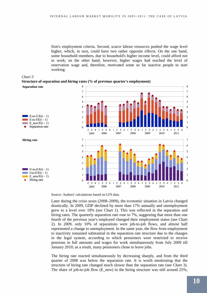
Worker mobility can be characterised by several measures, separation and hiring rates among them. We follow the notation used in Haltiwanger and Vodopivec (1999) and Meriküll (2011), and define the separation rate as the share of people employed one period ago (Et – 1) who separated from their employer either by entering unemployment (E-to-Ut) or inactivity (E-to-It) or due to finding a new employer (E_newt).
Separation rate = (E-to-Ut + E-to-It + E_newt)/Et – 1 (2.1).
The hiring rate is defined as the ratio of people who found a job and previously were either unemployed (U-to-Et) or inactive (I-to-Et), or worked with another employer (E_newt), to the number of people who were employed one period ago (Et – 1).
Hiring rate = (U-to-Et + I-to-Et + E_newt)/Et – 1 (2.2).
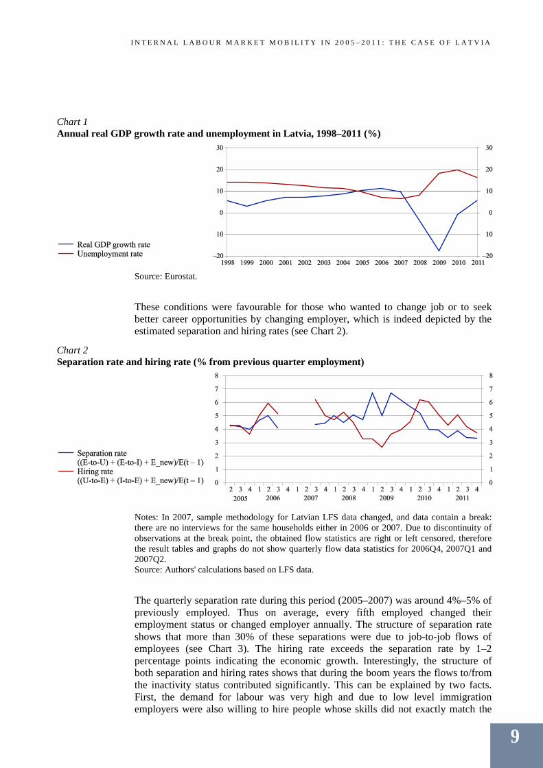
During 2005–2007, Latvia's economy was growing fast, GDP annual growth exceeded 9%, and the demand for labour was high; all these developments determined a relatively low level of unemployment (9.6% in 2005 and 7.3%–6.5% in 2006–2007; see Chart 1).
8
I N T E R N A L L A B O U R M A R K E T M O B I L I T Y I N 2 0 0 5 – 2 0 1 1 : T H E C A S E O F L A T V I A
Chart 1 Annual real GDP growth rate and unemployment in Latvia, 1998–2011 (%)
Source: Eurostat.
These conditions were favourable for those who wanted to change job or to seek better career opportunities by changing employer, which is indeed depicted by the estimated separation and hiring rates (see Chart 2).
Chart 2 Separation rate and hiring rate (% from previous quarter employment)
Notes: In 2007, sample methodology for Latvian LFS data changed, and data contain a break: there are no interviews for the same households either in 2006 or 2007. Due to discontinuity of observations at the break point, the obtained flow statistics are right or left censored, therefore the result tables and graphs do not show quarterly flow data statistics for 2006Q4, 2007Q1 and 2007Q2. Source: Authors' calculations based on LFS data.
The quarterly separation rate during this period (2005–2007) was around 4%–5% of previously employed. Thus on average, every fifth employed changed their employment status or changed employer annually. The structure of separation rate shows that more than 30% of these separations were due to job-to-job flows of employees (see Chart 3). The hiring rate exceeds the separation rate by 1–2 percentage points indicating the economic growth. Interestingly, the structure of both separation and hiring rates shows that during the boom years the flows to/from the inactivity status contributed significantly. This can be explained by two facts. First, the demand for labour was very high and due to low level immigration employers were also willing to hire people whose skills did not exactly match the
9
I N T E R N A L L A B O U R M A R K E T M O B I L I T Y I N 2 0 0 5 – 2 0 1 1 : T H E C A S E O F L A T V I A
firm's employment criteria. Second, scarce labour resources pushed the wage level higher, which, in turn, could have two rather opposite effects. On the one hand, some household members, due to household's higher income level, could afford not to work; on the other hand, however, higher wages had reached the level of reservation wage and, therefore, motivated some so far inactive people to start working.
Chart 3 Structure of separation and hiring rates (% of previous quarter's employment)
Source: Authors' calculations based on LFS data.
Later during the crisis years (2008–2009), the economic situation in Latvia changed drastically. In 2009, GDP declined by more than 17% annually and unemployment grew to a level over 18% (see Chart 1). This was reflected in the separation and hiring rates. The quarterly separation rate rose to 7%, suggesting that more than one fourth of the previous year's employed changed their employment status (see Chart 2). In 2009, only 10% of separations were job-to-job flows, and almost half represented a change to unemployment. In the same year, the flow from employment to inactivity remained substantial in the separation rate structure due to the changes in the legal system, according to which pensioners were restricted to receive pensions in full amounts and wages for work simultaneously from July 2009 till January 2010; as a result, many pensioners chose to leave jobs.
The hiring rate reacted simultaneously by decreasing sharply, and from the third quarter of 2008 was below the separation rate. It is worth mentioning that the structure of hiring rate changed much slower than the separation rate (see Chart 3). The share of job-to-job flow (E_new) in the hiring structure was still around 25%,
10
I N T E R N A L L A B O U R M A R K E T M O B I L I T Y I N 2 0 0 5 – 2 0 1 1 : T H E C A S E O F L A T V I A
while the share of flow from unemployed to employed (U-to-E) increased slightly. This indicates that part of those fired at the beginning of crisis were able to find new jobs quickly, i.e. without undergoing a long job search and drawing unemployment. As the crisis intensified, the aggregate number of unemployed increased, job search duration extended, and the share of the hired, who had previously been unemployed, increased. By the end of 2009, one third of the newly employed people were previously unemployed. The quite high share of job-to-job flow in hiring rate's structure can be explain by fragility of new worker-firm matches, i.e. a higher re-entry rate.
According to the estimates herein, the break point in negative trends of hiring and separation rates occurred in the middle of 2009, which is in line with the general tendencies of Latvia's economic recovery (see Chart 1 and Chart 2). The hiring rate bounced back to the boom years' level, and in the second quarter of 2010, exceeded the separation rate. Since then, the hiring rate has outpaced the separation rate, indicating economic recovery. Another sign of economic recovery is the growth of job-to-job flow (E_new) share in both separation and hiring rates. The share of flows from/to unemployment in 2011 remained higher than during the pre-crisis level, therefore the labour market adjustment process was still unfinished and a significant part of people were still looking for employment opportunities despite the fact that the hiring and separation rates had reached the pre-crisis level.
2.2 International comparison
Next, we provide comparison of Latvia with other European countries, which is of particular interest since labour flow statistics for Latvia are not present in major reports on the European labour market.
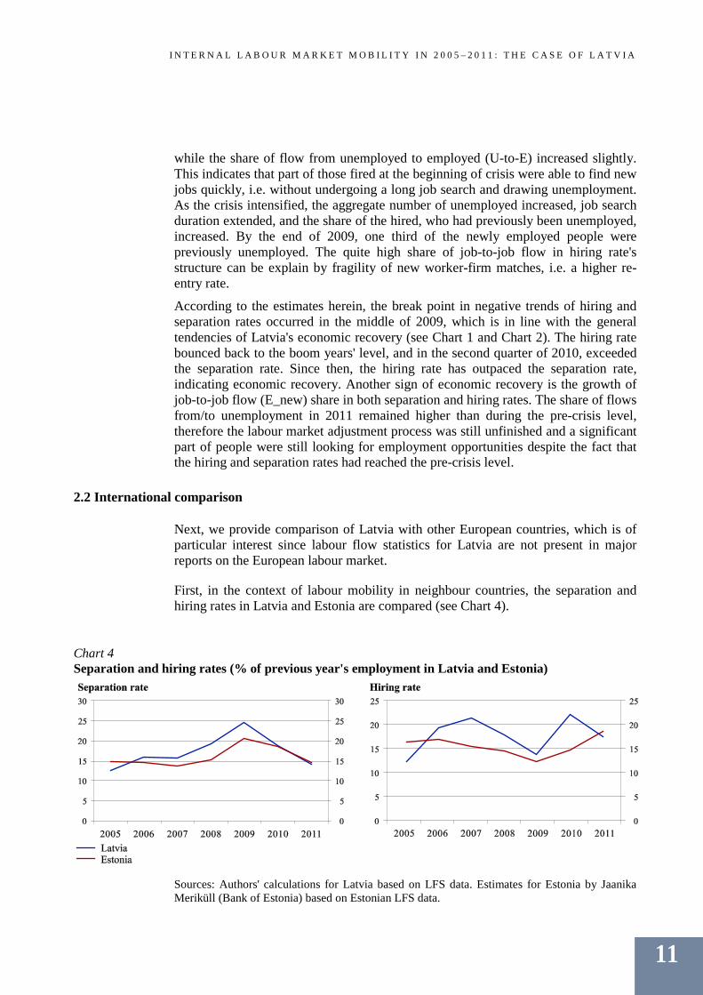
First, in the context of labour mobility in neighbour countries, the separation and hiring rates in Latvia and Estonia are compared (see Chart 4).
Chart 4 Separation and hiring rates (% of previous year's employment in Latvia and Estonia)
Sources: Authors' calculations for Latvia based on LFS data. Estimates for Estonia by Jaanika Meriküll (Bank of Estonia) based on Estonian LFS data.
11

I N T E R N A L L A B O U R M A R K E T M O B I L I T Y I N 2 0 0 5 – 2 0 1 1 : T H E C A S E O F L A T V I A
The separation and hiring rates for Estonia are constructed from LFS data using annual changes in labour market flows (see Meriküll (2011)). The results for two Baltic countries are not fully comparable due to differences in the estimation methodology. Nevertheless, it is useful to present annual estimates for two Baltic States together. According to these estimates, the worker reallocation rates in the two countries share common dynamics, i.e. separation and hiring rates amplified during the crisis in 2008–2009 and returned to the pre-crisis level in 2011. The conclusion that Latvia's worker reallocation rate is on average higher than that of the neighbouring country is confirmed if similar methodology as in Meriküll (2011) is used.
So far we have looked at the annual separation and hiring rates for Latvia and Estonia. The next logical step is to look at these two countries in the context of other European countries. There are several comparative research papers on labour flows using LFS micro data written by researchers of the European System of Central Banks (ESCB). As most recent examples, mention should be made of the ECB report (2012) on 13 euro area countries (Austria, Cyprus, Estonia, Spain, Finland, France, Greece, Ireland, Italy, Malta, the Netherlands, Slovenia and Slovakia) and a working paper of Spain's central bank written by Casado et al. (2012) for 11 EU countries (Austria, Belgium, Germany, Denmark, Spain, France, Greece, Italy, Portugal, Sweden and UK). The former presents quarterly results for individual countries and the aggregate for 13 euro area countries for two intervals: the pre-crisis period (2004Q1–2008Q2), and the crisis and post-crisis period (2008Q3–2010Q1). The latter provides annual results for individual countries for three periods: 2006–2008, 2009, and 2006–2009.
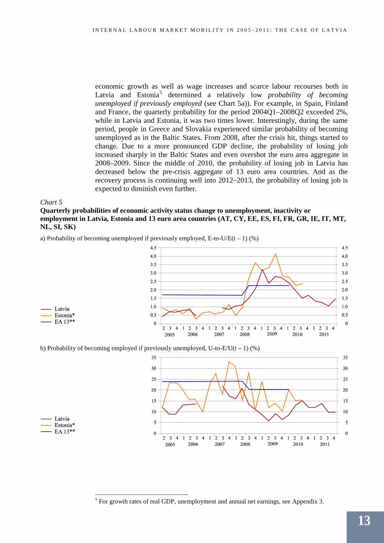
In the following section of research, we use the results provided in the ECB report (2012) due to longer coverage, quarterly representation of results, and similarities in the flow estimation approach3. We chose to present unconditional probabilities of economic status change in Latvia, Estonia and 13 euro area countries4; it is done by plotting the ratios of workers who changed their status vis-á-vis the corresponding number of employed, unemployed or inactive persons one period ago (see Chart 5). The estimates for 13 euro area countries are available only until 2010Q1.
Before describing the obtained results, we should stress that the presented probabilities are unconditional, i.e. the macroeconomic situation in respective countries is not taken into account. This section provides historical information on probabilities of changing the economic activity status in different countries. If one wants to compare labour mobility between countries, conditional probability should be used.
First, the quarterly probabilities of economic activity status change from employment are analysed. During the boom years (2006–2007), high rates of
3 In the ECB Structural issues report (2012), labour market status of individuals is tracked over the consecutive quarters during which they remain in LFS sample; therefore, labour flows are calculated from changes in the activity status of an individual between consecutive quarters. Retrospective questions are not taken into account. 4 The ECB Structural issues report (2012) on euro area labour markets contains both the estimates for individual countries and the aggregate value for 13 euro area countries. In order to keep the graph simple, only the aggregated value for 13 countries is presented.
12
I N T E R N A L L A B O U R M A R K E T M O B I L I T Y I N 2 0 0 5 – 2 0 1 1 : T H E C A S E O F L A T V I A
economic growth as well as wage increases and scarce labour recourses both in Latvia and Estonia5 determined a relatively low probability of becoming unemployed if previously employed (see Chart 5a)). For example, in Spain, Finland and France, the quarterly probability for the period 2004Q1–2008Q2 exceeded 2%, while in Latvia and Estonia, it was two times lower. Interestingly, during the same period, people in Greece and Slovakia experienced similar probability of becoming unemployed as in the Baltic States. From 2008, after the crisis hit, things started to change. Due to a more pronounced GDP decline, the probability of losing job increased sharply in the Baltic States and even overshot the euro area aggregate in 2008–2009. Since the middle of 2010, the probability of losing job in Latvia has decreased below the pre-crisis aggregate of 13 euro area countries. And as the recovery process is continuing well into 2012–2013, the probability of losing job is expected to diminish even further.
Chart 5 Quarterly probabilities of economic activity status change to unemployment, inactivity or employment in Latvia, Estonia and 13 euro area countries (AT, CY, EE, ES, FI, FR, GR, IE, IT, MT, NL, SI, SK) a) Probability of becoming unemployed if previously employed, E-to-U/E(t – 1) (%)
b) Probability of becoming employed if previously unemployed, U-to-E/U(t – 1) (%)
5 For growth rates of real GDP, unemployment and annual net earnings, see Appendix 3.
13
I N T E R N A L L A B O U R M A R K E T M O B I L I T Y I N 2 0 0 5 – 2 0 1 1 : T H E C A S E O F L A T V I A
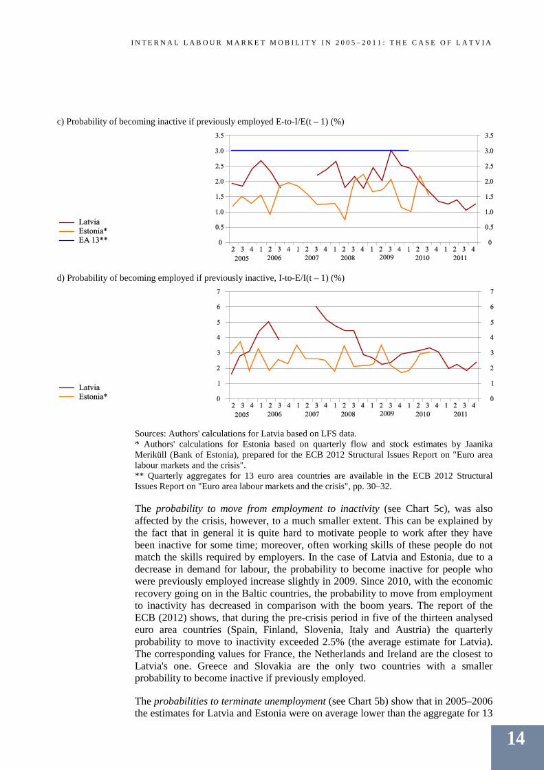
c) Probability of becoming inactive if previously employed E-to-I/E(t – 1) (%)
d) Probability of becoming employed if previously inactive, I-to-E/I(t – 1) (%)
Sources: Authors' calculations for Latvia based on LFS data. * Authors' calculations for Estonia based on quarterly flow and stock estimates by Jaanika Meriküll (Bank of Estonia), prepared for the ECB 2012 Structural Issues Report on "Euro area labour markets and the crisis". ** Quarterly aggregates for 13 euro area countries are available in the ECB 2012 Structural Issues Report on "Euro area labour markets and the crisis", pp. 30–32.
The probability to move from employment to inactivity (see Chart 5c), was also affected by the crisis, however, to a much smaller extent. This can be explained by the fact that in general it is quite hard to motivate people to work after they have been inactive for some time; moreover, often working skills of these people do not match the skills required by employers. In the case of Latvia and Estonia, due to a decrease in demand for labour, the probability to become inactive for people who were previously employed increase slightly in 2009. Since 2010, with the economic recovery going on in the Baltic countries, the probability to move from employment to inactivity has decreased in comparison with the boom years. The report of the ECB (2012) shows, that during the pre-crisis period in five of the thirteen analysed euro area countries (Spain, Finland, Slovenia, Italy and Austria) the quarterly probability to move to inactivity exceeded 2.5% (the average estimate for Latvia). The corresponding values for France, the Netherlands and Ireland are the closest to Latvia's one. Greece and Slovakia are the only two countries with a smaller probability to become inactive if previously employed.
The probabilities to terminate unemployment (see Chart 5b) show that in 2005–2006 the estimates for Latvia and Estonia were on average lower than the aggregate for 13
14
I N T E R N A L L A B O U R M A R K E T M O B I L I T Y I N 2 0 0 5 – 2 0 1 1 : T H E C A S E O F L A T V I A
euro area countries. During the period of fast real GDP growth and scarce labour force supply in 2007, the probability of becoming employed in Latvia and Estonia plummeted to 20% level and reached the average level of selected euro area countries. Before the crisis, the top five countries ranked by probability of becoming employed if previously unemployed, according to the ECB report (2012) were Austria, Spain, Cyprus, Finland and Slovenia (the average probability above 25%). During the crisis, the overall probability to find job in 13 euro area countries decreased (Spain, Slovenia and Ireland lost approximately 10 percentage points). Meanwhile, the drop in probability of finding job in Latvia and Estonia was of similar magnitude as in these three countries. During 2010–2011, the probability to find job if previously unemployed returned to the pre-crisis level in Latvia and Estonia.
During the analysed period, the quarterly probabilities of employment if previously inactive were around 3% in Latvia and Estonia (see Chart 5d). Interestingly, the estimates for Latvia present a pronounced effect of economic boom in 2006–2007, which is not observed for Estonia. The high demand for labour force along with the wage increase most probably had motivated people to move into employment, and the probability to become employed if previously inactive almost doubled. Unfortunately, we do not have aggregated data for 13 euro area countries for comparison, thus the relative size of the effect is not clear.
To sum up, the above provided analysis used unconditional probabilities and thus showed the historical situation, which was influenced by different macroeconomic conditions. In order to understand labour mobility better, a more detailed labour flow analysis is provided in the next sections.
2.3 Detailed labour flow analysis
In this section, we concentrate on internal labour mobility in Latvia. There are several topics we want to cover, among them full/part-time employment, permanent/temporary contracts, and mobility between regions, sectors and types of job.
Part time employment
The part-time job mechanism is important for labour market adjustment; it insures labour market flexibility and helps the economy absorb shocks. For example, during the time of economic crisis, the employer doesn't have to fire people, if he can reduce the number of working hours, and the unemployed person can easier find a part-time position and, hence, ensure some basic income level for the household.
15
I N T E R N A L L A B O U R M A R K E T M O B I L I T Y I N 2 0 0 5 – 2 0 1 1 : T H E C A S E O F L A T V I A
Chart 6 Share of part time employment in E-to-U, E-to-I, U-to-E, I-to-E and E_new flows
a) Flow from/to part-time job within job-to-job flow (% of job-to-job flow)
b) Flow from/to part-time job to/from unemployment and inactivity (% of corresponding flows)
Source: Authors' calculations for Latvia based on LFS data.
In 2005–2006 on average, 5% of job-to-job flows were flows to part-time employment (see Chart 6a). Since the beginning of the crisis, this number has skyrocketed, reaching 25% level in the second quarter of 2009 (estimates of the third and fourth quarters of 2009 are biased due to small sample). As the economy stabilised, so did the share of job-to-job flows to part-time employment. Therefore, we can conclude that the part-time employment mechanism was actively used in Latvia during the crisis. The opposite dynamics, i.e. flows to full-time employment from part-time employment, show that during the boom years the substitution to full-time employment was more pronounced than substitution to part-time employment (approximately 10%–15% of job-to-job flows were substitution from part-time to full-time positions), during the crisis this number dropped to 5%, and since 2010 the share has increased to the pre-crisis level of 10% on average. It is worth mentioning that during 2010 and 2011 the shares of flows to/from part-time employment are very similar, indicating a more balanced dynamics in the labour market than in the boom-bust period.
There is some asymmetry in flows to/from part-time jobs from/to unemployment and inactivity as shown in Chart 6b. On average 15% of people who were previously unemployed or inactive accept part-time positions. During the crisis this number increased to 25% and since 2010 has returned to 20% level. This indicates that,
16
I N T E R N A L L A B O U R M A R K E T M O B I L I T Y I N 2 0 0 5 – 2 0 1 1 : T H E C A S E O F L A T V I A
indeed, during the crisis years it was easier to find part-time job. We also check whether the tendency to fire part-time employees was more pronounced during the crisis. This hypothesis is not confirmed, since the share of unemployed or inactive of all people who were previously employed part-time is quite stable and does not depict clear cyclical behaviour. Thus we can conclude that employees working part or full-time were equally affected by job-cut policies during the crisis.
Temporary job contracts
Another labour market mechanism, which increases capacity of shock absorption through adjustment in labour market, is temporary job contracts. They allow for higher flexibility in employment decisions of firms, and decrease costs of firing people.
Chart 7 presents the shares of temporary contracts in Latvia for two groups of people: those, who were previously unemployed or inactive, and those who changed the employer.
Chart 7 Share of temporary contracts in U-to-E, I-to-E and E_new flows
Source: Authors' calculations for Latvia based on LFS data.
The obtained shares indicate that after the crisis Latvian employers are most probably more in favour of temporary contracts than before, i.e. the temporary contract mechanism became more widespread. By 2010, more than 15% of contracts signed when starting new jobs were temporary.
A similar tendency, i.e. an increase in the share of employees holding temporary contracts, was observed in other European countries. The ECB report (2012) indicates6 that in 10 euro area countries on average (France, Spain, Finland, Italy, the Netherlands, Slovenia, Slovakia, Austria, Greece and Estonia), this indicator increased from 7% in 2004Q1–2008Q2 to 9.5% in 2008Q3–2010Q1. The biggest increase in the share of temporary contracts was observed in Estonia (from 3.8% to 14.2%), Spain (from 7.5% to 14.3%), and Slovakia (from 4.5% to 10.5%).
6 ECB Structural Issues Report (2012) "On euro area labour markets and the crisis", p. 31, Chart 10.
17
I N T E R N A L L A B O U R M A R K E T M O B I L I T Y I N 2 0 0 5 – 2 0 1 1 : T H E C A S E O F L A T V I A
Internal geographical mobility
Further on, the paper provides the results on labour mobility within the regions of Latvia. The other aspect of geographical mobility, i.e. external mobility, is not within the scope of this research due to limited information on this matter in LFS.7
The study of internal labour mobility based on LFS data from 2004 by Paci et al. (2010) concludes that the internal migration rates in the new EU member states have been low compared to the EU158 and other advanced economies, and that internal mobility is not strongly responsive to unemployment and wage differentials. Analysing three Baltic States, Hazans (2003) concludes that internal migration in all three countries is rather high by international standards; however, it is not sufficient to adjust for regional disparities. According to Hazans (2004), the different outcomes in wage disparities reduction among regions can be explained by country-specific patterns of commuting (indicating that Latvia is more monocentric than the other Baltic States) as well as by educational and occupational composition of the commuting flows. Indeed, in the case of Latvia, there is a high variation in the income level and unemployment rates; however, as presented in Table 1, the majority of internal mobility takes place within two economically most developed regions – Riga (the capital) and Pierīga (suburbs of Riga).
Table 1 Structure of internal mobility between regions of Latvia (%)
Job-to-job flow (E_new) U-to-E + I-to-E flows Have not changed region of
work
Moved to Moved from Have not changed region of work
Moved to Moved from
Riga, Pierīga
Other regions
Riga, Pierīga
Other regions
Riga, Pierīga
Other regions
Riga, Pierīga
Other regions
2005 90 4 6 8 2 89 10 1 7 4 2006 82 15 3 9 9 90 9 1 5 5 2007 86 10 4 6 8 87 11 1 6 7 2008 85 11 4 11 4 85 13 2 7 9 2009 86 10 4 12 2 87 12 1 8 5 2010 82 10 7 13 4 91 9 0 5 4 2011 87 9 4 9 4 91 8 1 5 3
Note: In the case of U-to-E and I-to-E flows, we compare the region of residence while unemployed or inactive and the region where the person found a new job. Source: Authors' calculations for Latvia based on LFS data. Within job-to-job flows, approximately 15% of people changed their region of work, and this level didn't change significantly during the crisis. Two thirds of internal mobility took place within Riga and Pierīga. This value might seem high; nevertheless, due to close distances, it is quite usual that many people travel every
7 The reference literature on external labour mobility in the Baltic countries comprises Fic et al. (2011), Hazans and Philips (2011), Ester and Fouarge (2007), while for Latvia there is only research by the Ministry of Welfare (2007a) and Hazans (2007). 8Austria, Belgium, Denmark, Finland, France, Germany, Greece, Ireland, Italy, Luxembourg, the Netherlands, Portugal, Spain, Sweden and the UK.
18
I N T E R N A L L A B O U R M A R K E T M O B I L I T Y I N 2 0 0 5 – 2 0 1 1 : T H E C A S E O F L A T V I A
day from suburbs to work in the capital. Therefore, the switch of the place of work between these two regions doesn't necessarily imply a change of the place of residence.
The crisis effect is more pronounced in internal mobility of people who were previously unemployed or inactive. During 2008–2009, the number of people who found job in the region other than the residence region increased (counter-cyclical effect). The majority found a new job in Riga and Pierīga.
Mobility between sectors and job types
Before presenting the results, we want to stress that from the given analysis of mobility between sectors of the economy excluded are the people who just started working and do not have previous experience, since the flow statistics require knowledge of previous and current job type and sector. Consequently, the results presented in this section take into account only the people with some work experience.
Mobility of labour between sectors and job types behave pro-cyclically, opposite to mobility between regions. In Latvia, on average 55% of people in the job-to-job (E_new) flow change the sector of employment and 50% change the type of job (see Table 2). During the crisis, the share of people who changed the sector or type of job decreased. Similar results are shown for Estonia in Meriküll (2011).
Table 2 Structure of labour mobility between job type and sector in job-to-job (E_new) flow (%)
No change in job type and sector
Change in job type and sector
No change in sector, but change in job type
Change in sector, but no change in job type
2005 28 49 6 17 2006 22 46 12 20 2007 24 43 10 23 2008 32 38 13 17 2009 37 37 10 16 2010 29 32 12 26 2011 34 34 12 20
Source: Authors' calculations based on LFS data.
There can be several reasons for such behaviour. First, naturally, there is a smaller variety of vacancies during the crisis than in the boom years; second, people become more risk averse and try to accept jobs with a higher probability to remain employed after the end of probation period. We believe that the propensity to change the sector of employment might vary with the sector and economic cycle. In order to check this hypothesis, we present the shares of within industry job change, i.e. we show the share of people who remain employed within the same sector after changing employer (see Chart 8).
We use NACE Rev. 1.1 classification9 of sectors and differentiate between the job-to-job flow and flows from unemployment or inactivity to employment, since the
9 For NACE Rev. 1.1 abbreviations see Appendix 1.
19
I N T E R N A L L A B O U R M A R K E T M O B I L I T Y I N 2 0 0 5 – 2 0 1 1 : T H E C A S E O F L A T V I A
decision to look for a new job in a different sector might depend on person's current economic activity status. Agriculture is the only sector where the probability to become employed within the sector if you were previously unemployed, is higher. It can be partially explained by seasonality of employment in the sector and the fact that people employed in agriculture live in rural areas and receive lower than average income, therefore the financial means to move to another sector or region are limited, especially if they had been unemployed or inactive for some time.
Chart 8 Share of within industry job change in job-to-job flow (E_new) and share of within industry job change comparing the industry of previous employment (the one before unemployment or inactivity) with the current employment industry (U-to-E and I-to-E flows; NACE Rev. 1.1; %)
Job-to-job (E_new) flow
Flow from unemployment or inactivity to employment (U-to-E+I-to-E)
Source: Authors' calculations based on LFS data.
On average 40% of people do not change the sector of employment while changing employer, this number increased slightly after the crisis. There are three sectors, showing pronounced counter-cyclical behaviour of within industry job flow (mobility between sectors decreases, therefore mobility within sector increases). The strongest tendency to remain in the same sector is present in the public sectors (herein defined as L, M, N, i.e. public administration and defence; compulsory social security, education, and health and social work). At the beginning of crisis, over 70% of people who changed job and were recently employed in the public sector, found a new job within the same sector. However, with the introduction of austerity measures and reduction of the number of public sector employees in 2010, this tendency changed, and people had to look for another employment opportunity. The other two sectors with pronounced counter-cyclical behaviour are agriculture, and
20
I N T E R N A L L A B O U R M A R K E T M O B I L I T Y I N 2 0 0 5 – 2 0 1 1 : T H E C A S E O F L A T V I A
wholesale and retail trade. The counter-cyclical behaviour of employment flows within these sectors is much less pronounced in the case of previous unemployment or inactivity.
Construction (F), mining and quarrying, manufacturing and electricity, gas and water supply (C, D, E)10 as well as transport, storage and communication (I) sectors displayed pro-cyclical behaviour of within industry job flow during the crisis. The share of within sector job flows decreased due to an overall drop in demand and a sharp fall of housing prices, which forced temporary reduction in output and the number of employees. Consequently, people were forced to find a job in a different sector or to become unemployed.
The above presented findings confirm our hypothesis that propensity to change the sector of employment varies across sectors. Next, we would like to proceed with between sector mobility analysis (see Appendices 4 and 5). Appendix 4 displays the structure of worker inflows to and Appendix 5 the worker outflows from selected industries in Latvia, differentiating between flows to employment from either unemployment or inactivity (U-to-E and I-to-E) and job-to-job flows (E_new).
The first conclusion that can be drawn from the analysis of Appendix 4 is that the shares of inflow to sectors are not too different for previously employed and unemployed people; hence, people's decision to enter the sector (inflows into the sector) is driven by similar factors, e.g. higher wage level, job availability, etc. On the over hand, the discrepancies in the structure of outflows from sectors (see Appendix 5) for people with previously different status of employment are more pronounced, and thus the reasoning behind the decision to leave the sector might differ, e.g. a longer unemployment period might limit future employment opportunities.
The construction sector (F) is one of the typical examples of such outflow behaviour (see Appendix 5). The share of people who left construction industry (if previously unemployed or inactive) compared with the share of those who were recently employed (job-to-job flow) was much smaller during the boom years. This can be explained by the fact that, while the economy was rapidly growing, there was a constantly high demand for workers in construction, thus those with a lower skill level could find job in this sector. During the crisis, however, when the construction sector was severely hit and a huge part of workers were laid off, the outflow shares became similar. After the crisis, when the sector was gradually recovering, the tendencies changed, and presumably people with better skills were hired, hence the decreasing share of outflows from the construction sector for people in the job-to-job flow.
Another sector with specific outflow dynamics is agriculture (A, B). One can notice that in this sector, similar to the construction sector (F), the share of outflows of recently employed (E_new) was higher than the outflow of people who were working in the sector before becoming unemployed or inactive (U-to-E and I-to-E). This indicates that the corresponding sectors absorbed big shares of people with relatively low skills. These two sectors are also those with the most pronounced
10 In the further text we use shorter notation – manufacturing sector (C, D, E), transportation sector (I).
21
I N T E R N A L L A B O U R M A R K E T M O B I L I T Y I N 2 0 0 5 – 2 0 1 1 : T H E C A S E O F L A T V I A
change in the share of total worker outflows. As was shown above, the share of outflows from the construction sector exhibits pronounced cyclical behaviour; it increased sharply during the crisis and declined along with economic recovery. The share of outflows from agriculture decreased over time, indicating restructuring of the sector, e.g. an increase in intensity of production. The shares of worker outflows from the other sectors remained quite stable over time.
The tendencies in labour force inflows (see Appendix 4) confirm that in the construction sector they are pro-cyclical. Inflows to other sectors are less volatile, e.g. the inflow to manufacturing sector (C, D, E) was at around 15% of the total worker reallocation flow annually, and increased after 2010 due to improvements in competitiveness and expansion of exports (Benkovskis (2012)). The share of worker inflow to the wholesale and retail trade sector (G) during the crisis decreased to 15% of total worker reallocation as a result of wage cuts and a subsequent drop in the domestic demand for goods. The transportation sector (I), on the other hand, increased its share of employee inflow to 10% in 2009 due to relatively stable foreign demand and growing exports. The share of inflows to the public sector (L, M, N) increased during the boom years and decreased after the implementation of austerity measures and reduction of jobs in the public sector in 2010.
Before moving to the next part of our analysis, we would like to summarise some intermediate results. Unconditional probabilities show that the shares of worker flows from/to unemployment in Latvia and Estonia before the crisis were on average lower than in the reviewed 13 euro area countries; these flows became more similar during the crisis. The conducted detailed analysis of labour mobility in Latvia shows the following. First, in 2011, probability to exit unemployment or inactivity returned to the level of 2005–2006, and that to become inactive, if previously employed, decreased below the pre-crisis level, pointing to economic recovery. Second, the part-time and temporary contract mechanisms were actively used in Latvia, indicating flexibility of the labour market. Third, within region mobility in Latvia increased slightly during the crisis, behaving counter-cyclically, with the highest share of within region mobility between the capital and its suburbs (Riga region and Pierīga region). Fourth, during the crisis, the share of people who changed sector or job type decreased, thus mobility of labour between sectors and job types in Latvia behaved pro-cyclically. Finally, the labour inflow and outflow shares to different industries are not homogenous across industries and time.
These findings shape our interest to conduct more detailed analysis of labour mobility. Hence in the next section we control for several factors (region, industry, length of employment/unemployment, gender, education, age, marital status, registration with the State Employment Agency, etc.), in order to obtain the effect on probability to find or lose job. This way, the results can be used to provide recommendations how to improve labour mobility for employees with particular sets of characteristics.
22
I N T E R N A L L A B O U R M A R K E T M O B I L I T Y I N 2 0 0 5 – 2 0 1 1 : T H E C A S E O F L A T V I A
3. SURVIVAL ANALYSIS FOR LABOUR MARKET SPELLS
To explore Latvia's labour market in more detail, additional analysis of the length of labour market spells, i.e. time for person to change his/her economic activity status from/to employment to/from unemployment, and determinants of such changes, is provided here. In this section of the research, we first present the approach of Kaplan–Meier survival estimates to assess unconditional probability of change in the economic status, and then provide an explanation for the Cox PH model, which helps gain insights into determinants of labour market spell changes.
3.1 Kaplan–Meier survival estimates
The Kaplan–Meier (1958) estimator is a widely used nonparametric estimate of the survival function S(t) that indicates the probability of survival past time t. It describes time-to-event data. In the context of labour market, "survival" is understood as the period of time when an individual remains in the same labour market state, i.e. if the person is unemployed, the survival time is the period of unemployment, but if he/she is employed, it is the period of employment. The survival function is a function that describes these changes. Thus the Kaplan–Meier estimate at any time t is
∏≤
−=
ttj j
jj
jn
dntS
|
)(ˆ (3.1)
where jn is the number of individuals at risk at time jt , and jd is the number of failures at time jt . For labour market data "failure" is defined as a change of employment status (employed to unemployed or unemployed to employed, depending on changes analysed in each particular case).
Graphical representation of Kaplan–Meier survival function, e.g. spells from unemployment to employment (see, for example, Chart 9), shows the change in the share of people who have survived (in our case – remained unemployed) at moment t. Looking from another perspective, the survival curve shows how many months part of the unemployed sample (called the risk set) needed to find job.
The LFS database includes data on the state of economic activity (employed, unemployed or inactive) during the week of the interview and retrospective information about the time when person last left/found job. The retrospective information has monthly precision if the spell's length is less than two years. If the change of status took more than 2 years, the precision decreases, since in this case the interviewee only indicates the year when he/she last worked or became unemployed. In the calculations herein, therefore, the accuracy of length for long-term spells decreases. As people are interviewed several times, it is possible to follow information for an extended period of time and calculate the length of different spells. To make these calculations, a monthly-based dataset was formed, from which short term spells with periods less than one month were excluded.
The results of Kaplan–Meier survival estimate can be shown in graphs, which are used as the first step before creating hazard models. These graphs are just a general illustration of differences in survival rates of individuals with various characteristics.
23
I N T E R N A L L A B O U R M A R K E T M O B I L I T Y I N 2 0 0 5 – 2 0 1 1 : T H E C A S E O F L A T V I A
As in this case other factors are not controlled, some differences might be caused by other characteristics of these persons.
Further analysis will focus only on unemployment spells ending in employment. Unemployment spells ending in inactivity are not included, as retrospective questions do not provide information on unemployment to inactivity movements. First of all, as the observation period is quite long (2005–2011), it will be split in shorter periods in order to obtain estimates for different phases of the business cycle. This splitting was done on the basis of GDP growth data (from the CSB), defining the beginning of the crisis as a period when the GDP growth rates became negative year-on-year, but the end of the crisis as the time when they became positive. The respective periods are 2005Q1–2008Q2 (economic development), 2008Q3–2010Q2 (beginning of the crisis, economic slowdown), and 2010Q3–2011Q4 (recovery from the crisis, first signals of growth). Period-based partitioning of the dataset is a way to determine changes in labour mobility due to different business cycles.
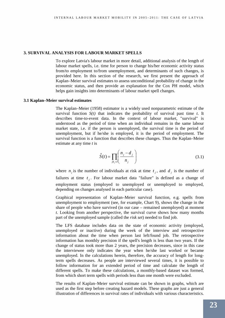
Chart 9 Survival function of unemployment spells (analysis time in months)
Notes: Years show the end time of the spell. Spells ending in other periods are excluded. Analysis time is in months. Source: Authors' calculations based on LFS data.
Chart 9 shows Kaplan–Meier survival curves for spell changes from unemployment to employment, where the horizontal axis represents the number of months the respondents remained unemployed, and the vertical axis captures the share of respondents who remained unemployed after t months. So, in the upper left corner all curves start at "1" representing 100% of people who were unemployed at moment t=0. Over time, the curves decrease as part of the unemployed find jobs. If the curve is located further up to the right, the spells of unemployment are longer. The lines in this graph represent the subsample of people who found a new job in the corresponding period, whereas the shaded area is the confidence interval of these indicators. So, for example, during the period's 2005Q1–2008Q2 and 2008Q3–2010Q2, 75% of the unemployed were still without job when the unemployment period had lasted already for 7 months. In the period 2010Q3–2011Q4, as the share of unemployed increased significantly in the total number of economically active population, it took more time (approximately 11 months) to achieve the same share of economic status change from unemployment to employment. It shows that during the crisis, the length of unemployment had accumulated, which subsequently had an impact on the flows from unemployment to employment in the next period.
24
I N T E R N A L L A B O U R M A R K E T M O B I L I T Y I N 2 0 0 5 – 2 0 1 1 : T H E C A S E O F L A T V I A
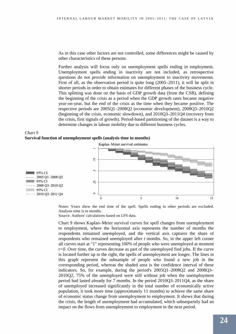
As Chart 9 shows, that similar to unemployment survival estimates for people who found job in the corresponding year we can provide unemployment survival estimates for those who lost job in the corresponding years (see Chart 10); in this case we split the dataset by years when a particular unemployment spell started. Those who entered unemployment during 2008Q3–2010Q2 were on average unemployed longer before finding job than those who became unemployed in the period 2005Q1–2008Q2; however, these differences are not statistically significant, as confidence intervals overlap, over longer time horizons in particular. Thus we can conclude that the crisis, in comparison with the period before it, has not led to a higher probability of a person becoming long-term unemployed. It had more impact on short-term unemployment, while over a longer time period the differences became insignificant, suggesting that the labour market was flexible and able to adjust to different conditions.
In order to avoid misunderstandings regarding the results, we should remember that Chart 10 includes the estimates only for such unemployment spells that have ended. The available unemployment spells for 2010Q3–2011Q4 are most likely right-censored (i.e. only those who found job quickly would be included in the sample); hence the results for the last period are biased and are not presented.
Chart 10 Survival function of unemployment spells (analysis time in months)
Notes: Years show the beginning time of the spell. Spells ending in other periods are excluded. Analysis time is in months. Source: Authors' calculations based on LFS data.
As shown in the graphs above, the labour market tendencies in different periods vary, therefore further analysis will concentrate not only on average tendencies for the entire seven-year period but also describe particular periods (pre-crisis, crisis, post-crisis) in more detail.
To check which variables should be explored in the further hazard model analysis, survival curves controlling for one factor describing respondents (gender, marital status, nationality and education) were constructed. These graphs are included in Appendix 6. It should be noted that in this case the results are not simultaneously controlled by the other factors (this will be done later in Cox PH model estimation). The survival curves show that each particular factor separately does not play statistically significant role in determining unemployment length. Though, women, married people and non-Latvians seem to have a bit longer unemployment durations.
25
I N T E R N A L L A B O U R M A R K E T M O B I L I T Y I N 2 0 0 5 – 2 0 1 1 : T H E C A S E O F L A T V I A
In order to obtain the direct effect of explanatory variables on changes in employment status, the Cox proportional hazards model is applied to the data on unemployment and employment spell changes. The methodology and results are presented in the following section.
3.2 Cox proportional hazards (PH) model
To explore which factors affect the probability of finding or losing job, and how their influence changes during a boom-bust period, the Cox proportional hazards (PH) model (Cox (1972)) was used. It is a mathematical model for analysing survival probabilities. The model shows the hazard of leaving a particular labour force state at period t. The Cox PH model can be written in the following form:
∑
= =
p
iii X
ethXth 1)(),( 0
β
(3.2) ),...,,( 21 pXXXX =
where X is the set of explanatory variables. Equation 3.2 shows the hazard which is the product of two quantities. The first is )(0 th , which is called the baseline hazard. The second (explicitly defined in equation 3.3) is the hazard ratio, which for each variable xi is written as:
𝐻𝑅𝑖 = 𝑒𝛽𝑖 (3.3).
The baseline hazard has no particular parameterisation and can be left unestimated, and the model makes no assumptions about the shape of the hazard over time, except for that these shapes of the hazard are the same for everyone. Explanatory variables X are time-independent, but the baseline hazard is a function of time. The Cox PH model has no intercept as it is subsumed into the baseline hazard )(0 th , i.e. it is unidentifiable from the data.
It should be noted that the model does not calculate the probability that the person will leave the risk set, but the ratio at which the hazard to leave the risk set for this individual is higher or lower than for those who are in the comparison set of individuals. The baseline hazard is left unestimated, but we receive information about the proportion of hazards for different groups of individuals.
The hazard ratio shows how many times the hazard of leaving the risk set at a particular period is larger for individuals with parameter xi than for other individuals. For the purpose of labour market analysis, the risk set will be either all of the employed or all of the unemployed, and the model will estimate the ratios of probabilities for individuals with different characteristics to change their labour force state.
As the labour force dataset is based on a sample, the quarterly weights are used to aggregate calculations for the whole population. Calculations are shown for full period (2005–2011) and shorter periods reflecting differences of various business cycle periods. These periods are 2005Q1–2008Q2, 2008Q3–2010Q2 and 2010Q3–2011Q4. The split is chosen to identify if the probability of loosing/finding job changes for different individuals in various time periods, for example, whether some of them are more vulnerable during the crisis, and what characteristics of individuals
26

I N T E R N A L L A B O U R M A R K E T M O B I L I T Y I N 2 0 0 5 – 2 0 1 1 : T H E C A S E O F L A T V I A
are appraised by employers. The results of these calculations could furnish policy makers with better understanding of factors behind longer unemployment spells for different groups of people and, thus, provide a baseline for labour market policy formation.
3.2.1 Determinants of employment to unemployment movement
The dynamics of labour market is reflected by people changing jobs, losing them and finding new ones. In all times, especially during the economic crisis, it is necessary to understand which groups of people are more likely to become unemployed. Therefore, there is a need to reflect on social protection of these groups and possibilities to increase their qualification and compliance with the labour market. Some of such policies are already in place (for example, protection of those on maternity leave, pre-pension age, etc.).
In this section, we provide an overview of the factors that determine the hazard of employed individuals to become unemployed. The results from the Cox PH model for the movement from employment to unemployment are shown in Appendix 7. They are compiled for a full data set and three smaller time periods reflecting different phases of Latvia's labour market.
It should be noted that the provided values are not probabilities themselves but the ratios of probabilities, meaning that if the number is above 1, the probability to lose job for a particular type of people is higher than for those in the comparison group. Vice versa, if the hazard ratio is below 1 and all other factors remain the same, the probability to lose job for a particular group of people is lower than for those in the comparison group. It is also important that hazard ratios show comparison with the average comparison group in a particular sub-set, therefore the hazard ratios of different periods (before, during and after the crisis) cannot be compared.
The results in this section are based on the sample of respondents who previously were employed and either remained employed or became unemployed. Therefore, the question about the time when a person left his/her previous job provides necessary information about the probability to change the employment status. A change in the data collection methodology after 2006 is one of the reasons why during 2005–2006 the number of observations is modest and why the number of respondents changing their job status from employed to unemployed is relatively small in comparison with the number of observations for further years.
In Appendix 7, we test whether such factors as gender, marital status, age, education, sector of employment, region of residence and length of employment can explain changes in the hazard of losing job. The first hypothesis tested is whether gender combined with person's marital status is a significant factor in explaining the movement from employment to unemployment. The effect of marital status could be connected with the presence of children in the family or the necessity to take care of other household members; hence these factors could influence the decision to either leave the job (to spend more time with family) or, on the contrary, to try to preserve it due to higher risk aversion during the crisis and the need to provide certain income level for the family. When the information about marital status is included in the model, the results are ambiguous. It cannot be stated if in general these groups are more or less likely to enter unemployment, and the hazard ratios are not statistically significant. It seems, however, that married women, if compared with single men,
27

I N T E R N A L L A B O U R M A R K E T M O B I L I T Y I N 2 0 0 5 – 2 0 1 1 : T H E C A S E O F L A T V I A
were less likely to lose their jobs before the crisis, which can be explained by extra social protection for women with kids.
The age structure analysis suggests that the hazard of losing job varies for different age groups of workers. So, the probability to become unemployed is higher for younger people, while that for people at pre-retirement age is lower in comparison with the group of middle-aged (35–44) employees. This effect doesn't change during the crisis, capturing the effect of social protection mechanism for pre-pension age workers.
One more significant factor determining the movement from employment to unemployment is the level of education. First estimations showed that for people with higher education the hazard of becoming unemployed is less likely. To get detailed information about which kind of higher education has the most positive effect, a model with both the level of education and the field of higher education was created (explanation of related abbreviations can be found in Appendix 1). Two types of higher education were specially examined, and they are higher education in social sciences and business as well as education of lower and higher level in more technologically oriented fields (engineering, manufacturing, construction, mathematics, statistics, and computing). Other higher education fields were not examined and more detailed analysis was not carried out as the number of observation for each type of education is low.
On average, people with higher education in social sciences have a relatively low probability to lose job in comparison with people with only secondary education. Also, it should be noted that after the crisis the demand for people with professional and vocational training increased. Therefore, the hazard to lose job for this group of employees decreased significantly, and during 2010Q3–2011Q4 they were less likely to be fired than those with secondary education.
Quite comprehensive information was obtained from the analysis of the impact of the sector of employment. We chose manufacturing as the baseline sector. In general, all other sectors exhibit a higher probability to lose job than manufacturing. During the boom years (2005Q1–2008Q2), workers' mobility from employment to unemployment was strong in the wholesale and retail trade sector, even though this sector was flourishing. This tendency can be explained by the overall high demand for labour in the sector at that time, and, hence, weaker resistance of employees to switch job or employer.
During the crisis, the output in all sectors of the Latvian economy decreased significantly. Accordingly, this resulted in a higher probability to lose job. However, since the hazard ratios capture relative increases in the probability to switch from employment to unemployment vis-a-vis the manufacturing sector and the crisis worsened the prospects to remain employed for all sectors, the effect of working in a particular sector remained similar to the pre-crisis level. The only difference is that the odds to switch from employment to unemployment in the wholesale and retail trade sector became similar to the other sectors. One of the most affected sectors during the crisis was construction. Also, the employment to unemployment flow during the crisis was relatively higher in public sector. As the public sector underwent severe reductions in the number of employed in 2010 and the possibility to further reduce the number of employees was limited, the relative probability of becoming unemployed for people working in the public sector decreased. After the
28
I N T E R N A L L A B O U R M A R K E T M O B I L I T Y I N 2 0 0 5 – 2 0 1 1 : T H E C A S E O F L A T V I A
crisis, as economy started to recover, the hazard of becoming unemployed in wholesale and retail trade diminished.
We also check whether, keeping all the other factors constant, the probability to lose job differs between the capital city and other regions. To do so, we use the division into three regions – Riga (the capital), Pierīga (suburbs of Riga) and the other regions11. In general, there is no evidence that the region of residence has any extra effect on the hazard of losing job.
Another significant determinant of probability to lose job is the length of employment. The risk to become unemployed is higher during the first year of employment. It can be explained by two factors, i.e. the probation time at a new job (in Latvia typically three months) and temporary or seasonal contracts. Moreover, people with previous longer work experience have lower hazard of losing job and, in the case of necessity to lay off some workers, those with shorter job tenure are chosen more frequently. If a person has been employed longer than a year, the probability to lose his/her current job strongly diminishes.
To promote a more complete understanding of labour mobility tendencies over different time periods, a movement, opposite to these employment to unemployment flows and describing tendencies of finding job is presented in the next section.
3.2.2 Determinants of unemployment to employment movement
This section presents the results of Cox PH model for flows from unemployment to employment. The hazard ratios in Appendix 8 show how the probability to find job differs for unemployed persons with different characteristics. Similar to the previous section, we check whether gender, marital status, education, region of residence or length of employment has any effect on the probability of finding job. Additionally we check whether registration with the State Employment Agency can be seen as an indicator of better job finding chances.
We will start with the effect of gender and marital status. According to the findings in other researches on labour mobility in Latvia, worker mobility does not significantly differ by gender (Ministry of Welfare (2007b), Hazans (2005)), but there is a gender wage gap in Latvia (Hazans (2007)). On the basis of calculations in this paper, we conclude that both single and married women are less likely to find job, but if they are employed, they are more likely to retain this status, while men change jobs more often. It is true, however, that this difference is not statistically significant for some periods, which would explain why some of the previous researches mention gender as having insignificant impact on worker mobility. According to our results, the situation differs for married women, for they are less likely to become employed. The gender effect was most pronounced during the crisis period (2008Q3–2010Q2). By contrast, the probability to find employment is higher for married men, which could be explained by the need to take care of their families.
Age figures as another factor that could influence individuals' choice to become employed (as well as employers' choice which employees to hire) despite the regulations that prohibit discrimination based on this factor. Economically active
11 A more detailed split does not display significant differences between regions.
29
I N T E R N A L L A B O U R M A R K E T M O B I L I T Y I N 2 0 0 5 – 2 0 1 1 : T H E C A S E O F L A T V I A
people aged 15–24 are more likely to become employed, and it is in line with the theory that young people are more mobile. The results of hazard model show that during the post-crisis period there were no significant differences between probabilities to switch from unemployment to employment for different age categories. In the crisis years, younger people were more likely to find jobs than middle-aged employees. The unemployment level in younger age groups is higher than on average. According to the CSB data, the unemployment rate for people aged 15–24 fluctuated around 30% level in 2009–2011, while the average unemployment rate in Latvia in this period was two times lower. Possibly due to this high unemployment rate young people were willing to enter employment under job contracts with less favourable conditions that would most likely be refused by older people with job experience. The results obtained for the post-crisis period (2010 Q3–2011 Q4) show that older people (aged 55–74) in comparison with the middle–aged people were more likely to find jobs. This is not a regular feature of the Latvian labour market, yet in this particular period the situation was caused by changes in the legal system: from July 2009 till January 2010, the restriction to simultaneously receive full pension and payment for work was imposed on pensioners. Therefore many retirees chose to quit jobs, but when this restriction was removed, some of them returned to the labour market, thus increasing the unemployment to employment flow.
During the pre-crisis period (2005 Q1–2008 Q2), when the demand for labour was very high, the level of education didn't have large influence on the probability to find a job. With the beginning of the crisis, the situation changed. As the number of job seekers increased, employers were more willing to employ workers with higher education. Since 2008, higher education in technical sciences has become an advantage in the labour market. The results of the model suggest that after the crisis, the effect of higher education on the probability to find job continued to be significant and even increased. It is important to mention that after 2010 Q3, people with professional education could change their status from unemployment to employment faster than people with only secondary education, which points to the economic recovery of the manufacturing sector.
There are some differences in probabilities to find jobs in different regions. Using information about the region of residence, we can conclude that the highest probability to find job is for people living in the capital city Riga. In Pierīga (suburbs of Riga), the probability to find job is on average by 20% smaller than in Riga. Similarly, in other regions the probability to find job was lower than in the capital.12 These effects remain similar in all periods explored.
Evaluating the effect of unemployment duration, we can say that the probability to find job decreases with unemployment length. After an unemployment spell of at least 6 months, the probability for a person to find job decreases by more than half in comparison with those who were unemployed for a shorter period (less than 6 months). After one year, the probability is only one fifth of that level. This can be explained by several factors. First of all, part of unemployment is on account of people who entered unemployment voluntarily, being sure of their possibilities to find job and of finding a better option. Another reason is that the best candidates are more likely to be selected for an open position faster, so their unemployment spell is
12 More detailed split by region does not show significant difference.
30
I N T E R N A L L A B O U R M A R K E T M O B I L I T Y I N 2 0 0 5 – 2 0 1 1 : T H E C A S E O F L A T V I A
shorter. Those who have been unemployed for more than six months are more likely to be less appealing to prospective employers. Another factor that could motivate people to find job early is the system of decreasing unemployment benefits. Family's financial situation can urge people to lower their standards for the job they are searching and take available vacancies quite early; those who are able to afford longer unemployment periods could still be picky, and they need more incentives to finally accept some job and start working.
Registration as unemployed with the State Employment Agency is a good indicator of higher probability (and maybe also willingness) of the person to find a job. For those who do not register with the Agency, the probability to find job is on average 0.76 times smaller than for persons who are registered. This factor is significant in all periods included in the analysis, yet after the crisis it lost its statistical significance.
The comparison of flow results from employment to unemployment and from unemployment to employment leads to the conclusion that worker mobility is influenced by both the economic situation in the country and specific characteristics of individual groups. That is why policies, aimed at protecting those with smaller employment probabilities and enhancing their job opportunities, are needed. As shown by the results above, the current legislation of social protection is already operating well for particular groups of employed (e.g. those on maternity leave, at pre-pension age or with longer job tenures), hence these groups of people are less likely to become unemployed. Nevertheless, more policy improvements are needed, especially with regard to providing better employment opportunities, as these groups of people are less likely to find employment (possibly because of both the skills mismatch and some discrimination by employers).
31

I N T E R N A L L A B O U R M A R K E T M O B I L I T Y I N 2 0 0 5 – 2 0 1 1 : T H E C A S E O F L A T V I A
CONCLUSIONS
Labour market in Latvia has proved to be flexible; it accelerated the economic recovery after the crisis and is presently enhancing Latvia's ability to adjust to asymmetric shocks not only through price but also labour market channels when Latvia joins the euro area.
The results of labour flow analysis suggest that labour flows adjust rapidly, indicating flexibility of firms' employment decisions reflected in the dynamics of separation and hiring rates. The mechanism of part-time employment and temporary contracts was actively used in Latvia during the crisis, attesting the flexibility of contract options; the labour market can adjust not only through reducing the number of employees but also through decreasing the number of hours worked or changing the contract type, thus reducing the costs of labour force adjustment. The hypothesis that people working part-time were fired more actively during the crisis is not confirmed. Thus we can conclude that employees working part- or full-time were equally affected by job-cut policies.
There is evidence of an increase in internal mobility between regions during the crisis (however, most internal mobility (two thirds of total flows) is on account of Riga and Pierīga and not between economically less developed regions and Riga). Mobility between sectors and job types, on the other hand, shows the signs of slowdown during the crisis most likely due to both smaller variety of vacancies and growing risk aversion of employees, which is in line with the results of other countries. It can also be concluded that the shares of labour inflow and outflow to/from different sectors are not homogenous and change over time. The most pro-cyclical behaviour is observed for the construction sector, since the sharp decline in the Latvian economy in 2008 was largely driven by the housing price bubble burst.
Two important signs of economic recovery after the financial crisis in Latvia should be emphasised: the probability to exit unemployment or inactivity returning to the level of 2005–2006, and the probability to become inactive if previously employed decreasing below the pre-crisis level. The unemployment duration analysis also suggests that the crisis in comparison with the pre-crisis period did not lead to a higher probability for inhabitants to become long-term unemployed. It suggests that the risk of hysteresis effect (high persistence of recent increase in unemployment) does not seem to be a long-term problem in Latvia.
Detailed information on probability to lose or find job was gained from the survival analysis. The research indicates that flows from/to employment to/from unemployment are determined by the characteristics of particular worker groups, performance of particular sectors of the economy, and the demand for particular level education or experience in specific fields. Probability to lose job is higher for those working with the current employer for less than one year and young people with elementary, professional and vocational education (except in recent years). Those working in the manufacturing sector or in the Riga region are less likely to enter unemployment. People with unemployment spells of less than 6 months, younger inhabitants, people with higher education, and in the post-crisis period also those with professional education can find jobs easier.
Contrary to some other EU countries, it is relatively easy for young people (aged up to 24) to find jobs in Latvia. Although they are also under high risk to lose their
32
I N T E R N A L L A B O U R M A R K E T M O B I L I T Y I N 2 0 0 5 – 2 0 1 1 : T H E C A S E O F L A T V I A
employment, employers are generally willing to hire young workers. The current social protection laws affecting particular groups of employees (e.g. those on maternity leave, at pre-pension age or with longer job tenure) operate well, and the results show that these groups of people are less likely to become unemployed. Yet, if they happen to lose their jobs, they are also less likely to find a new employment (possibly because of both the skills mismatch and some discrimination by employers).
Even if abstracting from external mobility and international labour flows, the labour market in Latvia has proved to be "internally" flexible. Internal and occupational migration, coupled with the flexibility of contract options and working hours, serve as a mobility boosting mechanism.
33

I N T E R N A L L A B O U R M A R K E T M O B I L I T Y I N 2 0 0 5 – 2 0 1 1 : T H E C A S E O F L A T V I A
APPENDIX 1 ABBREVIATIONS
Labour flow variables:
E-to-E, U-to-U, I-to-I – person who has not changed status (remained employed, unemployed or inactive) E-to-U – person who moved from employed to unemployed status U-to-E – person who moved from unemployed to employed status I-to-E – person who moved from inactive to employed status E-to-I – person who moved from employed to inactive status E(t – 1) – employment level at the beginning of the period
E(t – 1) = E-to-E + E-to-I + E-to-U E_new – person who remained employed but changed employer
Fields of higher education (based on Latvian education classification):
SOC – Social sciences, business and law TEH – Engineering, manufacturing, construction, mathematics, statistics and computing OTHER – all the other fields of higher education
NACE Rev. 1.1
Section Description A Agriculture, hunting and forestry B Fishing C Mining and quarrying D Manufacturing E Electricity, gas and water supply F Construction G Wholesale and retail trade; repair of motor vehicles, motorcycles and
personal and household goods H Hotels and restaurants I Transport, storage and communications J Financial intermediation K Real estate, renting and business activities L Public administration and defence; compulsory social security M Education N Health and social work O Other community, social and personal services activities P Activities of households Q Extra-territorial organisations and bodies
34

I N T E R N A L L A B O U R M A R K E T M O B I L I T Y I N 2 0 0 5 – 2 0 1 1 : T H E C A S E O F L A T V I A
APPENDIX 2 EXAMPLE OF OBTAINING QUARTERLY LABOUR FLOW AND STOCK STATISTICS FROM LFS LONGITUDINAL TYPE DATA
Economic activity matrix Weigth matrix Time Time
1 2 3 4 5 6 1 2 3 4 5 6 ID 1 E * * E ID 1 5 * * 6
2 E * U 2 7 * 9 3 U * * E 3 10 * * 11 4 U * U 4 1 * 1 5 E * * * E U 5 2 * * * 3 1
Probability U-to-E Probability E-to-U
ID 1 0 0 0 0 0 0 ID 1 0 0 0 0 0 0 2 0 0 0 0 0 0 2 0 0 0 0.5 0.5 0 3 0 0 0 0.333 0.333 0.333 3 0 0 0 0 0 0 4 0 0 0 0 0 0 4 0 0 0 0 0 0 5 0 0 0 0 0 0 5 0 0 0 0 0 1
Cumulative probability U-to-E (U→E) Cumulative probability E-to-U (E→U)
ID 1 0 0 0 0 0 0 ID 1 0 0 0 0 0 0 2 0 0 0 0 0 0 2 0 0 0 0.5 1 0 3 0 0 0 0.333 0.667 1 3 0 0 0 0 0 0 4 0 0 0 0 0 0 4 0 0 0 0 0 0 5 0 0 0 0 0 0 5 0 0 0 0 0 1
Cumulative probability U-to-E (U←E) Cumulative probability E-to-U (E←U)
ID 1 0 0 0 0 0 0 ID 1 0 0 0 0 0 0 2 0 0 0 0 0 0 2 0 0 1 0.5 0 0 3 0 0 1 0.667 0.333 0 3 0 0 0 0 0 0 4 0 0 0 0 0 0 4 0 0 0 0 0 0 5 0 0 0 0 0 0 5 0 0 0 0 1 0
35
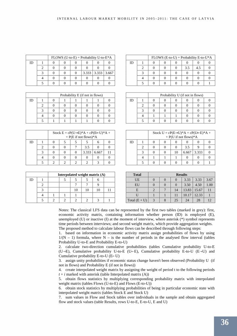
I N T E R N A L L A B O U R M A R K E T M O B I L I T Y I N 2 0 0 5 – 2 0 1 1 : T H E C A S E O F L A T V I A
FLOWS (U-to-E) = Probability U-to-E*A FLOWS (E-to-U) = Probability E-to-U*A
ID 1 0 0 0 0 0 0 ID 1 0 0 0 0 0 0 2 0 0 0 0 0 0 2 0 0 0 3.5 4.5 0 3 0 0 0 3.333 3.333 3.667 3 0 0 0 0 0 0 4 0 0 0 0 0 0 4 0 0 0 0 0 0 5 0 0 0 0 0 0 5 0 0 0 0 0 1
Probability E (if not in flows) Probability U (if not in flows)
ID 1 0 1 1 1 1 0 ID 1 0 0 0 0 0 0 2 0 0 0 0 0 0 2 0 0 0 0 0 0 3 0 0 0 0 0 0 3 0 0 0 0 0 0 4 0 0 0 0 0 0 4 1 1 1 0 0 0 5 1 1 1 1 0 0 5 0 0 0 0 0 0
Stock E = cP(U→E)*A + cP(E←U)*A +
+ P(E if not flows)*A Stock U = cP(E→U)*A + cP(U←E)*A +
+ P(U if not flows)*A ID 1 0 5 5 5 6 0 ID 1 0 0 0 0 0 0
2 0 0 7 3.5 0 0 2 0 0 0 3.5 9 0 3 0 0 0 3.333 6.667 11 3 0 0 10 6.667 3.333 0 4 0 0 0 0 0 0 4 1 1 1 0 0 0 5 2 2 2 2 3 0 5 0 0 0 0 0 1
Interpolated weight matrix (A) Total Results
ID 1 5 5 5 6 UE 0 0 0 3.33 3.33 3.67 2 7 7 9 EU 0 0 0 3.50 4.50 1.00 3 10 10 10 11 E 2 7 14 13.83 15.67 11 4 1 1 1 U 1 1 11 10.17 12.33 1 5 2 2 2 2 3 1 Total (E + U) 3 8 25 24 28 12
Notes: The classical LFS data can be represented by the first two tables (marked in grey): first, economic activity matrix, containing information whether person (ID) is employed (E), unemployed (U) or inactive (I) at the moment of interview, where asterisk (*) symbol represents time periods between interviews; and second weight matrix, which provide aggregation weights. The proposed method to calculate labour flows can be described through following steps: 1. based on information in economic activity matrix assign probabilities of flows by using 1/(N – 1) formula, where N – is the number of periods in the analysed flow interval (tables Probability U-to-E and Probability E-to-U) 2. calculate two-direction cumulative probabilities (tables Cumulative probability U-to-E (U→E), Cumulative probability U-to-E (U←E), Cumulative probability E-to-U (E→U) and Cumulative probability E-to-U (E←U) 3. assign unity probabilities if economic status change haven't been observed (Probability U (if not in flows) and Probability E (if not in flows)) 4. create interpolated weight matrix by assigning the weight of period t to the following periods t + i marked with asterisk (table Interpolated matrix (A)) 5. obtain flows statistics by multiplying corresponding probability matrix with interpolated weight matrix (tables Flows (U-to-E) and Flows (E-to-U)) 6. obtain stock statistics by multiplying probabilities of being in particular economic state with interpolated weight matrix (tables Stock E and Stock U) 7. sum values in Flow and Stock tables over individuals in the sample and obtain aggregated flow and stock values (table Results, rows U-to-E, E-to-U, E and U)
36
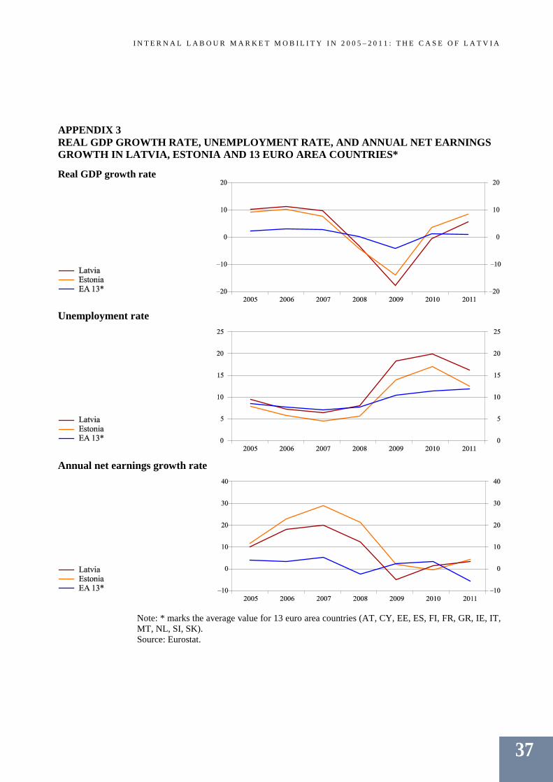
I N T E R N A L L A B O U R M A R K E T M O B I L I T Y I N 2 0 0 5 – 2 0 1 1 : T H E C A S E O F L A T V I A
APPENDIX 3 REAL GDP GROWTH RATE, UNEMPLOYMENT RATE, AND ANNUAL NET EARNINGS GROWTH IN LATVIA, ESTONIA AND 13 EURO AREA COUNTRIES*
Real GDP growth rate
Unemployment rate
Annual net earnings growth rate
Note: * marks the average value for 13 euro area countries (AT, CY, EE, ES, FI, FR, GR, IE, IT, MT, NL, SI, SK). Source: Eurostat.
37
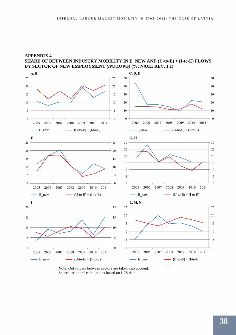
I N T E R N A L L A B O U R M A R K E T M O B I L I T Y I N 2 0 0 5 – 2 0 1 1 : T H E C A S E O F L A T V I A
APPENDIX 4 SHARE OF BETWEEN INDUSTRY MOBILITY IN E_NEW AND (U-to-E) + (I-to-E) FLOWS BY SECTOR OF NEW EMPLOYMENT (INFLOWS) (%; NACE REV. 1.1)
Note: Only flows between sectors are taken into account. Source: Authors' calculations based on LFS data.
38
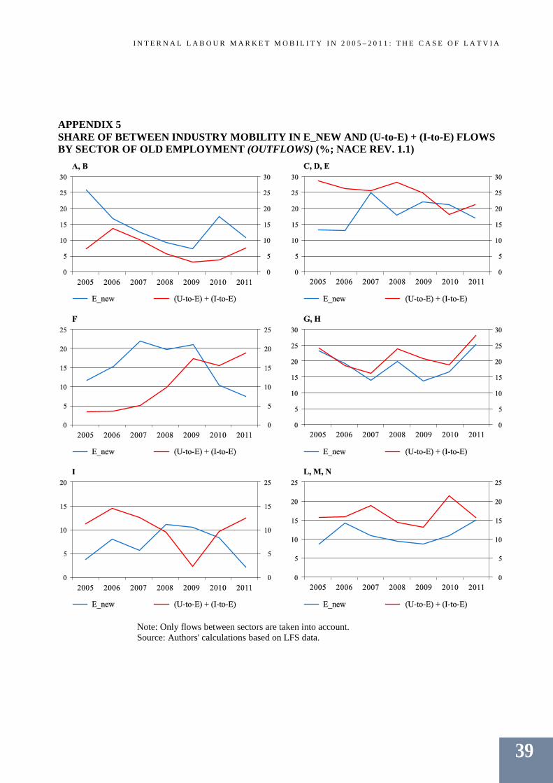
I N T E R N A L L A B O U R M A R K E T M O B I L I T Y I N 2 0 0 5 – 2 0 1 1 : T H E C A S E O F L A T V I A
APPENDIX 5 SHARE OF BETWEEN INDUSTRY MOBILITY IN E_NEW AND (U-to-E) + (I-to-E) FLOWS BY SECTOR OF OLD EMPLOYMENT (OUTFLOWS) (%; NACE REV. 1.1)
Note: Only flows between sectors are taken into account. Source: Authors' calculations based on LFS data.
39
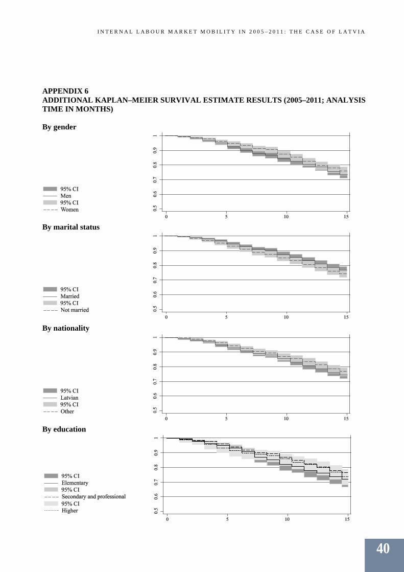
I N T E R N A L L A B O U R M A R K E T M O B I L I T Y I N 2 0 0 5 – 2 0 1 1 : T H E C A S E O F L A T V I A
APPENDIX 6 ADDITIONAL KAPLAN–MEIER SURVIVAL ESTIMATE RESULTS (2005–2011; ANALYSIS TIME IN MONTHS) By gender
By marital status
By nationality
By education
40
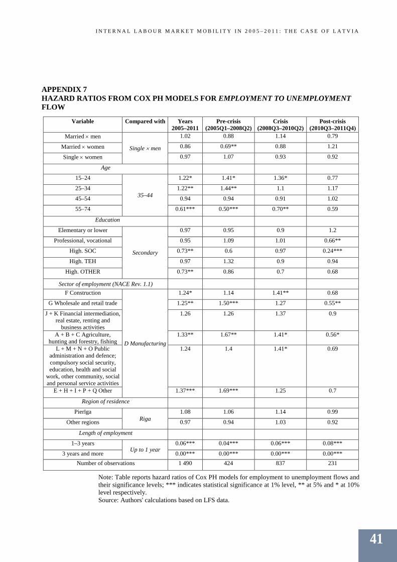
I N T E R N A L L A B O U R M A R K E T M O B I L I T Y I N 2 0 0 5 – 2 0 1 1 : T H E C A S E O F L A T V I A
APPENDIX 7 HAZARD RATIOS FROM COX PH MODELS FOR EMPLOYMENT TO UNEMPLOYMENT FLOW
Variable Compared with Years 2005–2011
Pre-crisis (2005Q1–2008Q2)
Crisis (2008Q3–2010Q2)
Post-crisis (2010Q3–2011Q4)
Married × men
Single × men
1.02 0.88 1.14 0.79
Married × women 0.86 0.69** 0.88 1.21
Single × women 0.97 1.07 0.93 0.92
Age
15–24
35–44
1.22* 1.41* 1.36* 0.77
25–34 1.22** 1.44** 1.1 1.17
45–54 0.94 0.94 0.91 1.02
55–74 0.61*** 0.50*** 0.70** 0.59
Education
Elementary or lower
Secondary
0.97 0.95 0.9 1.2
Professional, vocational 0.95 1.09 1.01 0.66**
High. SOC 0.73** 0.6 0.97 0.24***
High. TEH 0.97 1.32 0.9 0.94
High. OTHER 0.73** 0.86 0.7 0.68
Sector of employment (NACE Rev. 1.1) F Construction
D Manufacturing
1.24* 1.14 1.41** 0.68
G Wholesale and retail trade 1.25** 1.50*** 1.27 0.55**
J + K Financial intermediation, real estate, renting and
business activities
1.26 1.26 1.37 0.9
A + B + C Agriculture, hunting and forestry, fishing
1.33** 1.67** 1.41* 0.56*
L + M + N + O Public administration and defence; compulsory social security, education, health and social
work, other community, social and personal service activities
1.24 1.4 1.41* 0.69
E + H + I + P + Q Other 1.37*** 1.69*** 1.25 0.7
Region of residence
Pierīga Riga
1.08 1.06 1.14 0.99
Other regions 0.97 0.94 1.03 0.92
Length of employment
1–3 years Up to 1 year
0.06*** 0.04*** 0.06*** 0.08***
3 years and more 0.00*** 0.00*** 0.00*** 0.00*** Number of observations 1 490 424 837 231
Note: Table reports hazard ratios of Cox PH models for employment to unemployment flows and their significance levels; *** indicates statistical significance at 1% level, ** at 5% and * at 10% level respectively. Source: Authors' calculations based on LFS data.
41
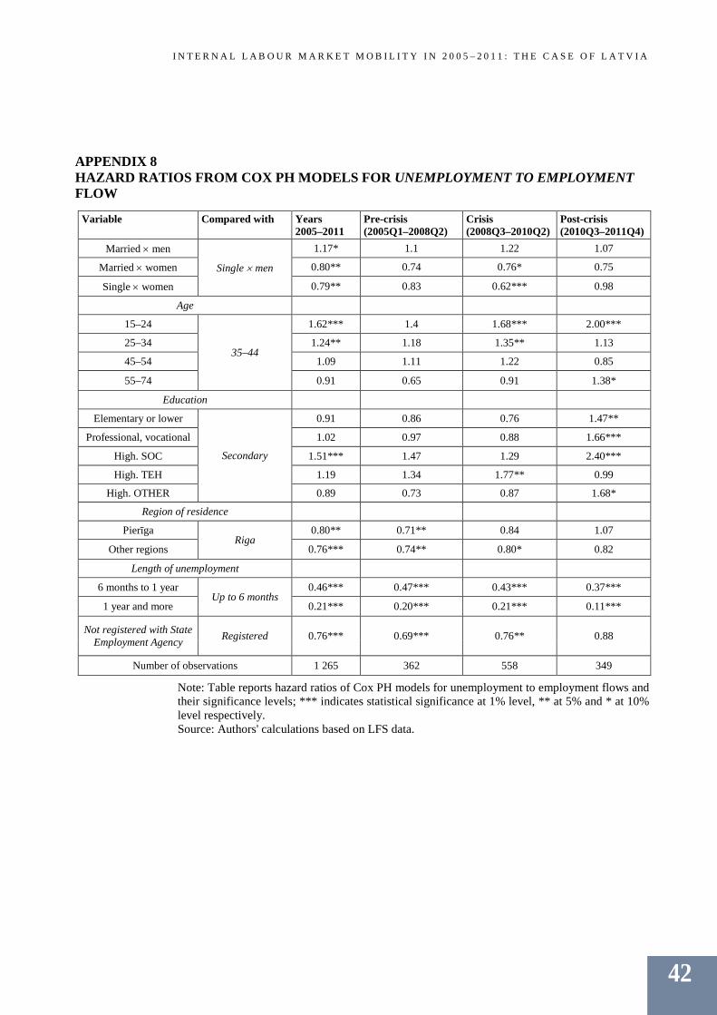
I N T E R N A L L A B O U R M A R K E T M O B I L I T Y I N 2 0 0 5 – 2 0 1 1 : T H E C A S E O F L A T V I A
APPENDIX 8 HAZARD RATIOS FROM COX PH MODELS FOR UNEMPLOYMENT TO EMPLOYMENT FLOW
Variable Compared with Years 2005–2011
Pre-crisis (2005Q1–2008Q2)
Crisis (2008Q3–2010Q2)
Post-crisis (2010Q3–2011Q4)
Married × men
Single × men
1.17* 1.1 1.22 1.07
Married × women 0.80** 0.74 0.76* 0.75
Single × women 0.79** 0.83 0.62*** 0.98
Age
15–24
35–44
1.62*** 1.4 1.68*** 2.00***
25–34 1.24** 1.18 1.35** 1.13
45–54 1.09 1.11 1.22 0.85
55–74 0.91 0.65 0.91 1.38*
Education
Elementary or lower
Secondary
0.91 0.86 0.76 1.47**
Professional, vocational 1.02 0.97 0.88 1.66***
High. SOC 1.51*** 1.47 1.29 2.40***
High. TEH 1.19 1.34 1.77** 0.99
High. OTHER 0.89 0.73 0.87 1.68*
Region of residence
Pierīga Riga
0.80** 0.71** 0.84 1.07
Other regions 0.76*** 0.74** 0.80* 0.82
Length of unemployment
6 months to 1 year Up to 6 months
0.46*** 0.47*** 0.43*** 0.37***
1 year and more 0.21*** 0.20*** 0.21*** 0.11***
Not registered with State Employment Agency Registered 0.76*** 0.69*** 0.76** 0.88
Number of observations 1 265 362 558 349
Note: Table reports hazard ratios of Cox PH models for unemployment to employment flows and their significance levels; *** indicates statistical significance at 1% level, ** at 5% and * at 10% level respectively. Source: Authors' calculations based on LFS data.
42
I N T E R N A L L A B O U R M A R K E T M O B I L I T Y I N 2 0 0 5 – 2 0 1 1 : T H E C A S E O F L A T V I A
BIBLIOGRAPHY
ARTOLA, Concha, BELL, Una-Louise (1999) – Identifying Labour Market Dynamics Using Labour Force Survey Data. Banco de España Working Paper, No. 9922, December. 44 p. BEŅKOVSKIS, Konstantīns (2012) – Competitiveness of Latvia's Exporters. Baltic Journal of Economics, Baltic International Centre for Economic Policy Studies, vol. 12, issue 2, pp. 17–45. BLANCHARD, Olivier, DIAMOND, Peter A. (1992) – The Flow Approach to Labor Markets. American Economic Review, vol. 82, issue 2, pp. 354–359. CASADO, José Maria, FERNÁNDEZ-VIDAURRETA, Cristina, JIMENO, Juan F. (2012) – Labour Flows in the EU at the Beginning of the Crisis. Banco de España Economic Bulletin, January, pp. 91–101. COX, David R. (1972) – Regression Models and Life-Tables. Journal of the Royal Statistical Society. Series B (Methodological), vol. 34, No. 2, pp. 187–220. DAVIS, Steven J., HALTIWANGER, John (1998) – Measuring Gross Worker and Job Flows. In: Labour Statistics Measurment Issues. Ed. by J. Haltiwanger, M. E. Manser and R. Topel. University of Chicago Press, pp. 77–122. DAVIS, Steven J., HALTIWANGER, John (1999) – Gross Job Flows. In: Handbook of Labor Economics. Ed. by O. Ashenfelter and D. Card. North-Holland, Amsterdam, EconPapers, vol. 3, ch. 41, pp. 2711– 2805. ELSBY, Michael W., SMITH, Jennifer C., WADSWORTH, Jonathan (2011) – The Role of Worker Flows in the Dynamics and Distribution of UK Unemployment. Oxford Review of Economic Policy, Oxford University Press, vol. 27, No. 2, Summer, pp. 338–363. ESTER, Peter, FOUARGE, Didier (2007) – International and Regional Migration Intentions in Europe. Eurofound, Report No. ef0709, June. 53 p. European Central Bank (2012) – Euro area labour markets and the crisis. Structural Issues Report, October, pp. 28–39. FIC, Tatiana, HOLLAND, Dawn, PALUCHOWSKI, Pawel, et al. (2011) – Labour Mobility within the EU – The Impact of Enlargement and the Functioning of the Transitional Arrangements. National Institute of Economic and Social Research Discussion Paper, No. 379, Revised Version: August. 144 p. FLEK, Vladislav, MYSÍKOVÁ, Martina (2012) – Unemployment Dynamics in Central Europe: A Labor Flow Approach. Working Papers Institute of Economic Studies, Charles University Prague, No. 2012/07, March. 25 p. HALTIWANGER, John, VODOPIVEC, Milan (1999) – Gross Worker and Job Flows in a Transition Economy: An Analysis of Estonia. World Bank Policy Research Working Paper, No. 2082, November. 73 p. HAZANS, Mihails (2003) – Determinants of Inter-Regional Migration in the Baltic Countries. University of Bonn ZEI Working Papers, No. B 17-2003. 38 p. HAZANS, Mihails (2004) – Does Commuting Reduce Wage Disparities? Growth and Change, vol. 35, No. 3. Special Issue on Commuting, Summer, pp. 360–390.
43
I N T E R N A L L A B O U R M A R K E T M O B I L I T Y I N 2 0 0 5 – 2 0 1 1 : T H E C A S E O F L A T V I A
HAZANS, Mihails (2005) – Unemployment and the Earnings Structure in Latvia. World Bank Policy Research Working Paper, No. 3504, February. 90 p. HAZANS, Mihails (2007) – Coping with Growth and Emigration: Latvian Labor Market Before and After EU Accession [cited 3 May 2013]. Available: http://ssrn.com/abstract=971198. HAZANS, Mihails, PHILIPS, Kaia (2011) – The Post-Enlargement Migration Experience in the Baltic Labor Markets. IZA (Institute for the Study of Labor) Discussion Papers, No. 5878, July. 49 p. JANIAK, Alexandre, WASMER, Etienne (2008) – Mobility in Europe – Why it is Low, the Bottlenecks and the Policy Solutions. European Commision Economic Papers, No. 340, September. 157 p. JENKINS, Jamie, CHANDLER, Mark (2010) – Labour Market Gross Flows Data from the Labour Force Survey. Economic & Labour Market Review, vol. 4, issue 2, February. 25 p. KAPLAN, Edward L., MEIER, Paul (1958) – Nonparametric Estimation from Incomplete Observations. Journal of the American Statistical Association, vol. 53, No. 282, June, pp. 457–481. KUHLENKASPER, Torben, STEINHARDT, Max Friedrich (2011) – Unemployment Duration in Germany – A Comprehensive Study with Dynamic Hazard Models and P-Splines. NORFACE MIGRATION Discussion Paper, No. 2011-18, October. 35 p. MERIKÜLL, Jaanika (2011) – Labour Market Mobility During a Recession: the Case of Estonia. Eesti Pank Working Paper, No. 1/2011. 44 p. PACI, Pierella, TIONGSON, Erwin R., WALEWSKI, Mateusz, et al. (2010) – Internal Labour Mobility in Central Europe and the Baltic Region: Evidence from Labour Force Surveys. In: The Labour Market Impact of the EU Enlargement. A New Regional Geography of Europe? Ed. by F. E. Caroleo and F. A. Pastore. Berlin Heidelberg : Springer-Verlag, pp. 197–225. PISSARIDES, Christopher, LAYARD, Richard, HELLWIG, Martin (1986) – Unemployment and Vacancies in Britain. Economic Policy, vol. 1, No. 3, October, pp. 499–559. The Geographic Mobility of the Labour Force (2007a) – The National Programme of European Union Structural Funds, "Labour Market Research" the Project "Welfare Ministry Research". Riga : University of Latvia. 271 p. The Occupational Mobility of the Labour Force (2007b) – The National Programme of European Union Structural Funds, "Labour Market Researches" the Project "Researches of the Ministry of Welfare". Riga : University of Latvia. 241 p. ZASOVA, Anna, MEĻIHOVS, Aleksejs (2005) – Assessment of Labour Market Elasticity in Latvia. Bank of Latvia Working Paper, No. 3/2005. 59 p.
44