Embed Size (px)
Citation preview
INTERMEDIATION IN NETWORKS
MIHAI MANEA
Department of Economics, MIT, [email protected]
Abstract. We study intermediation in markets with an underlying network structure.
A good is resold via successive bilateral bargaining between linked intermediaries until it
reaches one of several buyers in the network. We characterize the resale values of all traders
in the network. The seller’s profit depends not only on the number of intermediaries involved
in trade, but on the entire set of competing paths of access to buyers brokered by each
intermediary. Local competition shapes the outcomes of intermediation. A decomposition
of the network into layers of intermediation power describes the endogenous structure of
local monopolies and trading paths. Local competition permits full profit extraction in
transactions within the same layer, while hold-up problems impose intermediation rents on
exchanges across layers. Layers delimit monopoly power from intermediation power. Only
players who serve as gateways to lower layers earn significant profits. Resale values decline
exponentially with each progressive layer. Trade does not maximize welfare or minimize
intermediation. We provide comparative statics with respect to the network architecture
and the distribution of intermediation costs. The elimination of a middleman and vertical
integration increase the seller’s profit, as does the transfer of costs downstream; horizontal
integration has ambiguous effects.
1. Introduction
Intermediation plays an important role in many markets. In corrupt and bureaucratic insti-
tutions, bribes are shared through long chains of intermediaries in the hierarchical structure.
Lobbyists gain access to powerful lawmakers by navigating the network of political connec-
tions and rewarding well-connected individuals for their influence and contacts. Illegal goods
such as drugs and unregistered guns are also smuggled and dealt through networks of in-
termediaries. Financial institutions resell complex assets over the counter through networks
of trusted intermediaries. Varying levels of intermediation are needed to bring agricultural
goods from small farms to the tables of final consumers. Artwork and antiques are sold via
the personal contacts of collectors and middlemen. Manufacturing in supply chains can also
be regarded as a form of intermediation, whereby a number of firms sequentially transforms
and resells a good until it becomes a finished product.
Date: December 22, 2014.I thank Daron Acemoglu, Glenn Ellison, Drew Fudenberg, Ben Golub, Jerry Green, Matt Jackson, FuhitoKojima, David Miller, Ben Olken, Michael Ostrovsky, and Jean Tirole for useful comments. I am alsograteful to Gabriel Kreindler for careful proofreading.
2 MIHAI MANEA
In such markets there exist competing intermediation paths between sellers and buyers
with a complex pattern of overlaps. The number of middlemen, the cost of intermediation,
and the value of final consumers may vary across trading paths. Some market participants
have access to more middlemen than others, who themselves enjoy a greater or smaller
number of connections. Clearly, not all links are equally useful in generating intermediation
rents. The bargaining power of each intermediary depends on both his distance to buyers
and the nature of local competition among his available trading routes. The global network
of connections among various intermediaries plays an essential role in determining the path
of trade and the profits that buyers, sellers, and middlemen achieve.1 Some fundamental
questions arise: How does an intermediary’s position in the network affect his intermediation
rents? Which players earn substantial profits? What trading paths are likely to emerge?
How can upstream players exploit downstream competition? Is intermediation efficient?
Does trade proceed along the shortest path? How does the seller’s profit respond to changes
in the network architecture such as the elimination of a middleman and the vertical or
horizontal integration of intermediaries?
Given the prevalence of networks in markets where trade requires the services of mid-
dlemen, it is important to develop non-cooperative models of intermediation in networks.
Decentralized bilateral bargaining is at the heart of our opening examples. Without at-
tempting to model closely any of those applications, this paper starts building the tools for
a non-cooperative theory of dynamic bilateral bargaining among buyers, sellers, and inter-
mediaries.2 We study the following intermediation game. A seller is endowed with a single
unit of an indivisible good, which can be resold via successive bilateral bargaining between
linked intermediaries in a directed network until it reaches one of several buyers. Intermedi-
aries have heterogeneous transaction costs and buyers have heterogeneous values. At every
stage in the game, the current owner of the good selects a bargaining partner among his
downstream neighbors in the network. The two traders negotiate the price of the good via
a random proposer protocol. With probability p, the current seller makes an offer and the
partner decides whether to acquire the good at the proposed price. Roles are reversed with
probability 1 − p. In either event, if the offer is rejected, the seller keeps possession of the
good and gets a new chance to select a partner at the next stage. If the offer is accepted,
then the seller incurs his cost and the two traders exchange the good at the agreed price. If
the new owner is an intermediary, he is given the opportunity to resell the good to his down-
stream neighbors according to the same protocol. Buyers simply consume the good upon
purchase. Players have a common discount factor. The main part of our analysis focuses
1Chapter 11 of Easley and Kleinberg (2010) provides an extensive discussion on the importance of interme-diation in networks.2We defer the discussion of the related literature to Section 11. It is worth noting at this point that the onlyother existing models of intermediation in networks via bilateral bargaining, proposed by Gale and Kariv(2007) and Condorelli and Galeotti (2012), consider strategic interactions quite distinct from ours.
INTERMEDIATION IN NETWORKS 3
on limit Markov perfect equilibria (MPEs) of the intermediation game as players become
patient.
To gain some intuition for the competitive forces induced by the chosen bargaining pro-
tocol, we start with the simple version of the model in which there are no intermediaries. In
this special case, a seller bargains over the price of the good with a number of heterogeneous
buyers. We prove that the bargaining game with no intermediaries has an essentially unique
MPE, which achieves asymptotic efficiency as players become patient (Proposition 1). The
limit MPE outcome is determined as though the seller can choose between two scenarios: (1)
a bilateral monopoly settlement whereby the seller trades only with the highest value buyer
and receives a share p of the proceeds; and (2) a second-price auction, in which the seller
exploits the competition between top buyers and extracts the entire surplus generated by
the second highest value buyer. In effect, the seller is able to take advantage of competition
among buyers and demand more than the bilateral monopoly share from the first-best buyer
only if the threat of trading with the second-best buyer is credible.
Consider next an MPE of the general intermediation game. We refer to a trader’s equilib-
rium payoff conditional on having possession of the good as his resale value. The strategic
situation faced by a current seller in the intermediation game reduces to a bargaining game
with his downstream neighbors, who can be viewed as surrogate buyers with valuations for
the good endogenously derived from their resale values in the MPE. This situation resembles
the game with no intermediation, with one critical distinction: the current seller’s trading
partners may resell the good to one another, directly or through longer paths in the network.
When the seller trades with a neighbor, other neighbors may still enjoy positive continuation
payoffs upon purchasing the good subsequently in the subgame with the new owner. Such
lateral intermediation rents act as endogenous outside options for the neighbors. A crucial
step in the analysis establishes that these outside options are not binding in equilibrium:
neighbors prefer buying the good directly from the current seller rather than acquiring it
through longer intermediation chains. This finding leads to a recursive characterization of
limit resale values. A key theoretical result proves that the resale value of any current seller
is derived in the limit as though his downstream neighbors were final consumers in the game
without intermediation with valuations given by their resale values (Theorem 1).
However, lateral intermediation rents influence the path of trade even when players are
arbitrarily patient. We show by example that the current seller may trade with positive limit
probability with partners who do not deliver the highest limit resale value (Remark 5). This
finding conflicts with the intuition from the special case with no intermediation, where the
seller trades with the highest value buyers almost surely in the limit. We also establish the
existence of MPEs (Proposition 2).
4 MIHAI MANEA
To examine in more detail the effect of an intermediary’s position in the network on his
resale value, we isolate network effects from other asymmetries by assuming that there are no
intermediation costs and buyers have a common value v. In such settings, any intermediary
linked to two (or more) buyers wields his monopoly power to extract the full surplus of v
in the limit. Moreover, any current seller linked to a pair of players known to have limit
resale value v also exploits the local competition to obtain a limit price of v. The process of
identifying players with a limit resale value of v continues until no remaining trader is linked
to two others previously pinned down. We label the pool of players recognized in the course
of this procedure as layer 0. The recursive characterization of resale values implies that any
remaining intermediary linked to a single layer 0 player has a limit resale value of pv. We
can then find additional traders who demand a limit price of pv due to competition among
the latter intermediaries, and so on.
Building on the arguments above, we develop an algorithm that decomposes the network
into a series of layers of intermediation power. Having defined layers 0 through ` − 1, the
construction of layer ` proceeds as follows. The first members of layer ` are those players
who are directly connected to layer ` − 1 and have not yet been assigned to a layer. Then
the remaining traders with at least two links to established members of layer ` join the layer.
Players linked to a pair of existing members of layer ` are also added to the layer, and so on.
Our main result shows that a trader’s intermediation power depends on the number of layer
boundaries the good crosses to reach from the trader to a buyer. Specifically, all players
from layer ` have a limit resale value of p`v. Moreover, even for positive costs, the network
decomposition leads to a uniform upper bound of p`v for the limit resale values of layer `
traders, as well as lower bounds that are close to p`v when costs are small (Theorem 2).
The characterization of resale values by means of the layer decomposition reveals that a
seller’s intermediation power is not only a function of the number of intermediaries needed
to reach buyers, but also depends on the competition among intermediation chains. Indeed,
layers measure the effective intermediation distance between players. In sparse networks with
insufficient local competition, such as line networks and square lattices, the initial seller’s
profits decline exponentially with the distance to buyers. However, in denser networks with
many alternate trading paths, such as triangular grids and small world networks, sellers
arbitrarily far away from buyers capitalize on long chains of local monopolies and earn
substantial profits.
Our network decomposition has implications for optimal network design in applications.
The initial seller sets trade in motion only if his cost does not exceed the maximum resale
value of his bargaining partners. Hence trade is possible only if the seller belongs to a
sufficiently low layer. Therefore, in manufacturing, agriculture, and financial markets, where
production and trade are beneficial, denser networks with short paths, strong downstream
INTERMEDIATION IN NETWORKS 5
competition, and extensive vertical integration are efficient. Such features allow the seller to
extract an adequate share of the gains from trade to cover his costs. However, in markets
where trade is not desirable, as in the case of bribery and illegal goods, sparser networks
with long paths and a lack of downstream competition are preferable. In such networks, low
profits may deter the seller from producing the (bad) good.
Although our bargaining protocol generates an asymptotically efficient MPE allocation in
the absence of intermediation, we find that the possibility of resale may create inefficiencies
(Proposition 4). We distinguish between two types of asymptotic inefficiency in the interme-
diation game. One type of inefficiency stems from hold-up problems created by the bilateral
nature of intermediation coupled with insufficient local competition. A seller facing weak
downstream competition is unable to charge a price close to the maximum resale value of his
neighbors and has to surrender substantial intermediation rents to his chosen partner. The
anticipation of such downstream rents reduces the gains from trade in upstream transactions
and may make trade unprofitable even when positive surplus is available along some inter-
mediation chains. The other type of intermediation inefficiency results from intermediaries’
incentives to exploit local competition. Equilibrium trading paths capitalize on local mo-
nopolies, and this is not generally compatible with global surplus maximization. Relatedly,
we find that in settings with homogeneous intermediation costs and a single buyer, trade
does not always follow the shortest route from the seller to the buyer. This finding refutes
the standard intuition that sellers have incentives to minimize intermediation.
We next investigate which intermediaries make significant profits. In settings with zero
costs and homogeneous values, a player earns positive limit profits only following acquisitions
in which he provides a gateway to a lower layer (Proposition 5). Thus layers delimit monopoly
power from intermediation power. Full profit extraction is possible in agreements within the
same layer, while intermediation rents are awarded in transactions across layers.
We also provide comparative statics with respect to the network architecture and the
cost distribution. The addition of a new link to the network weakly increases the initial
seller’s limit profit, as does the elimination of a middleman (Proposition 6). In our context,
eliminating a middleman entails a rewiring of the network whereby the middleman is removed
and upstream neighbors for whom the middleman provides critical intermediation in the
original network inherit his downstream links as well as his costs.
To discuss the effects of vertical and horizontal integration, we restrict attention to tier
networks.3 We show that the vertical integration of two consecutive tiers weakly increases
the limit profit of the initial seller (Proposition 7.1). The intuition is that the vertical in-
tegration of a pair of tiers amounts to the simultaneous elimination of all middlemen from
the downstream tier. However, we find that the horizontal integration of a pair of same-tier
3Tier networks provide a natural framework for integration. Formal definitions can be found in Section 9.We emphasize that tiers do not correspond to (endogenous) layers of intermediation power.
6 MIHAI MANEA
intermediaries has ambiguous effects on the initial seller’s welfare (Proposition 7.2). Horizon-
tal integration exerts countervailing forces on upstream and downstream competition. The
consolidated intermediary gains access to the joint pool of trading partners of the merging
players, which may enhance downstream competition and generate a higher resale value. At
the same time, horizontal integration eliminates competition between merged intermediaries
and leaves upstream neighbors with fewer bargaining opportunities.
Finally, we provide comparative statics with respect to the distribution of costs in a
fixed network. We establish that any downward redistribution of costs in the network can
only benefit the initial seller (Theorem 3). This result has ramifications for optimal cost
allocation in applications. In the case of bribery, lobbying, or illegal trade, an intermediary’s
transaction cost reflects the risk of getting caught red-handed. Crime can be prevented by
shifting monitoring efforts and the severity of punishments towards the top of the hierarchy.
In manufacturing, costs account for both production expenses and taxes. Our analysis
suggests that costs should be transferred downstream for efficient production. Hence retail
sales taxes are more efficient than value-added taxes, and subsidies are more effective in the
initial stages of production.
The study of intermediation in networks constitutes an active area of research. Section
11 discusses some important contributions to this literature. The distinguishing feature of
the present model is that it fully endogenizes competition among trading paths via strategic
choices at each step. That, in turn, determines prices and intermediation rents, and finally
delivers the layer structure of endogenous intermediation routes. The competition effects we
identify in our framework are novel to the literature.
The rest of the paper is organized as follows. Section 2 introduces the intermediation game
and discusses several interpretations and applications of the model. In Section 3, we analyze
the version of the game without intermediation. Section 4 provides the recursive charac-
terization of resale values in the intermediation game. The characterization is exploited in
Section 5 to establish the relationship between intermediation power and the network de-
composition into layers. The sources of intermediation inefficiencies are examined in Section
6. Section 7 investigates the division of intermediation profits. In Sections 8-10, we present
the comparative statics results. Section 11 reviews the related literature, and Section 12
concludes. Proofs omitted in the body of the paper are available in the Appendix.
2. The Intermediation Game
A set of players N = {0, 1, . . . , n} interacts in the market for a single unit of an indivisible
good. The good is initially owned by player 0, the initial seller. Players i = 1,m are
intermediaries (m < n). We simply refer to each player i = 0,m as a (potential) seller.
INTERMEDIATION IN NETWORKS 7
c0
c1 c2 c3
c4 c6c5 c7
v9 v10
c8
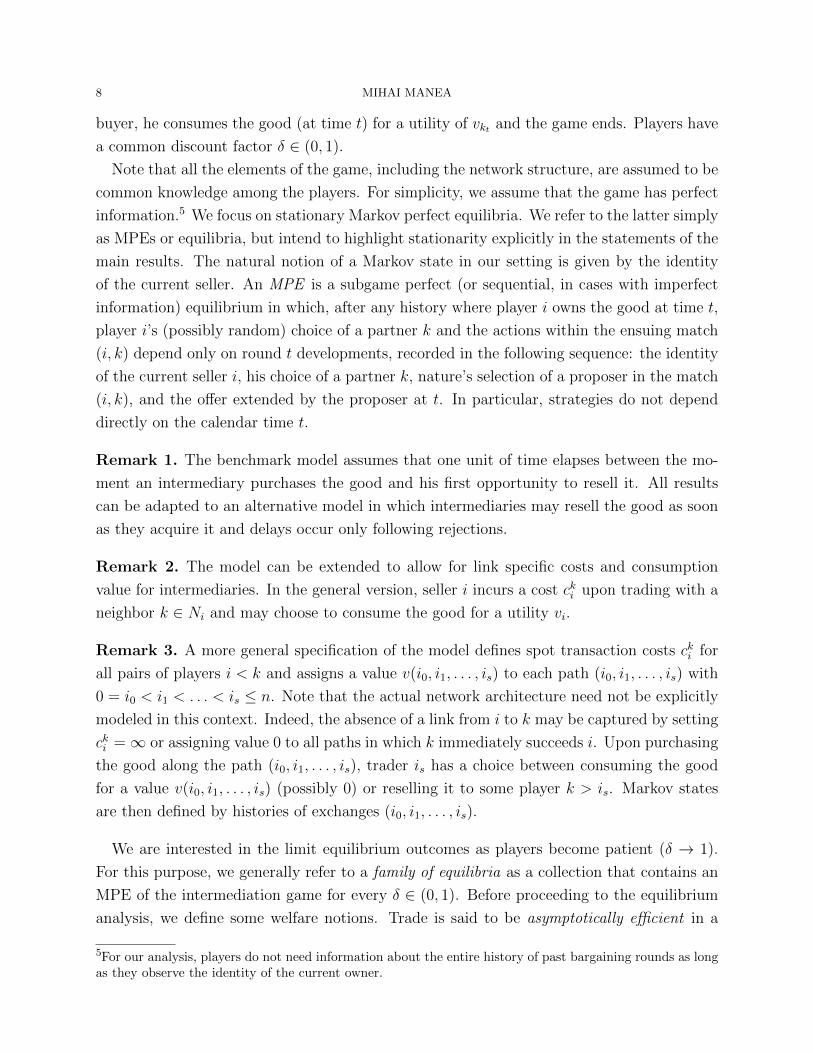
Figure 1. Network example
Every seller i = 0,m has a transaction or production cost ci ≥ 0. Each player j = m+ 1, n
is a buyer with a consumption value vj ≥ 0 for the good.4
Players are linked by a network G = (N, (Ni)i=0,m, (ci)i=0,m, (vj)j=m+1,n). Formally, G is a
directed acyclic graph with vertex set N . Each seller i = 0,m has out-links to “downstream”
players in the set Ni ⊂ {i+1, . . . , n}. Hence a link is an ordered pair (i, k) with k ∈ Ni. In the
intermediation game to be introduced shortly, Ni represents the set of players to whom the
current owner i can directly (re)sell the good. A trading path is a directed path connecting
the initial seller to a buyer, i.e., a sequence of players i0, i1, . . . , is with i0 = 0,m+1 ≤ is ≤ n,
and is ∈ Nis−1 for all s = 1, s. Without loss of generality, we assume that every player lies
on a trading path and that buyers do not have out-links. For fixed m < n, we refer to any
profile (Ni)i=0,m that satisfies the properties above as a linking structure.
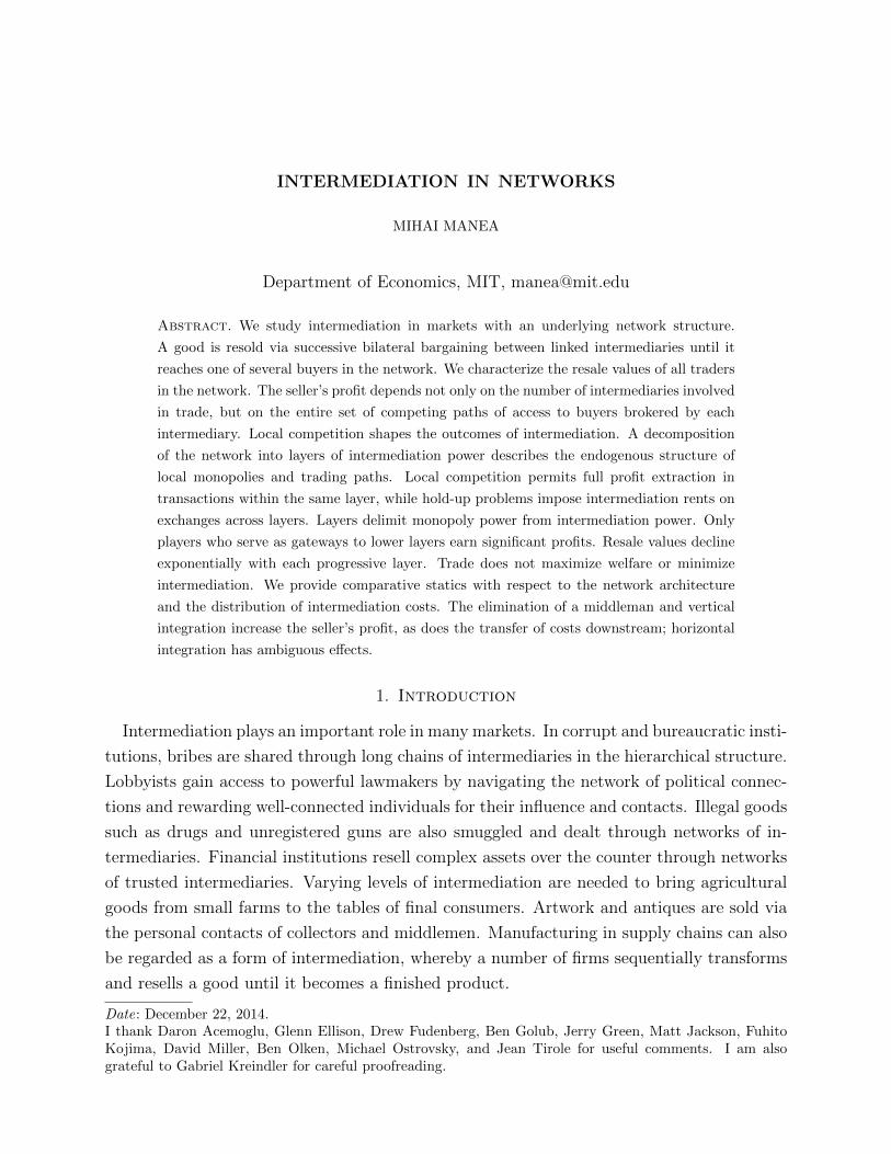
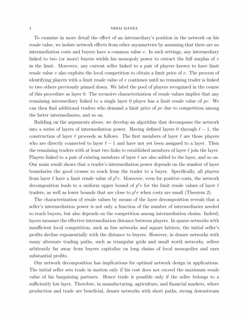
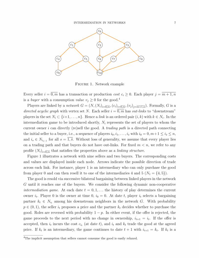
Figure 1 illustrates a network with nine sellers and two buyers. The corresponding costs
and values are displayed inside each node. Arrows indicate the possible direction of trade
across each link. For instance, player 1 is an intermediary who can only purchase the good
from player 0 and can then resell it to one of the intermediaries 4 and 5 (N1 = {4, 5}).The good is resold via successive bilateral bargaining between linked players in the network
G until it reaches one of the buyers. We consider the following dynamic non-cooperative
intermediation game. At each date t = 0, 1, . . . the history of play determines the current
owner it. Player 0 is the owner at time 0, i0 = 0. At date t, player it selects a bargaining
partner kt ∈ Nit among his downstream neighbors in the network G. With probability
p ∈ (0, 1), the seller it proposes a price and the partner kt decides whether to purchase the
good. Roles are reversed with probability 1− p. In either event, if the offer is rejected, the
game proceeds to the next period with no change in ownership, it+1 = it. If the offer is
accepted, then it incurs the cost cit (at date t), and it and kt trade the good at the agreed
price. If kt is an intermediary, the game continues to date t + 1 with it+1 = kt. If kt is a
4The implicit assumption that sellers cannot consume the good is easily relaxed.
8 MIHAI MANEA
buyer, he consumes the good (at time t) for a utility of vkt and the game ends. Players have
a common discount factor δ ∈ (0, 1).
Note that all the elements of the game, including the network structure, are assumed to be
common knowledge among the players. For simplicity, we assume that the game has perfect
information.5 We focus on stationary Markov perfect equilibria. We refer to the latter simply
as MPEs or equilibria, but intend to highlight stationarity explicitly in the statements of the
main results. The natural notion of a Markov state in our setting is given by the identity
of the current seller. An MPE is a subgame perfect (or sequential, in cases with imperfect
information) equilibrium in which, after any history where player i owns the good at time t,
player i’s (possibly random) choice of a partner k and the actions within the ensuing match
(i, k) depend only on round t developments, recorded in the following sequence: the identity
of the current seller i, his choice of a partner k, nature’s selection of a proposer in the match
(i, k), and the offer extended by the proposer at t. In particular, strategies do not depend
directly on the calendar time t.
Remark 1. The benchmark model assumes that one unit of time elapses between the mo-
ment an intermediary purchases the good and his first opportunity to resell it. All results
can be adapted to an alternative model in which intermediaries may resell the good as soon
as they acquire it and delays occur only following rejections.
Remark 2. The model can be extended to allow for link specific costs and consumption
value for intermediaries. In the general version, seller i incurs a cost cki upon trading with a
neighbor k ∈ Ni and may choose to consume the good for a utility vi.
Remark 3. A more general specification of the model defines spot transaction costs cki for
all pairs of players i < k and assigns a value v(i0, i1, . . . , is) to each path (i0, i1, . . . , is) with
0 = i0 < i1 < . . . < is ≤ n. Note that the actual network architecture need not be explicitly
modeled in this context. Indeed, the absence of a link from i to k may be captured by setting
cki =∞ or assigning value 0 to all paths in which k immediately succeeds i. Upon purchasing
the good along the path (i0, i1, . . . , is), trader is has a choice between consuming the good
for a value v(i0, i1, . . . , is) (possibly 0) or reselling it to some player k > is. Markov states
are then defined by histories of exchanges (i0, i1, . . . , is).
We are interested in the limit equilibrium outcomes as players become patient (δ → 1).
For this purpose, we generally refer to a family of equilibria as a collection that contains an
MPE of the intermediation game for every δ ∈ (0, 1). Before proceeding to the equilibrium
analysis, we define some welfare notions. Trade is said to be asymptotically efficient in a
5For our analysis, players do not need information about the entire history of past bargaining rounds as longas they observe the identity of the current owner.
INTERMEDIATION IN NETWORKS 9
family of equilibria if the sum of ex ante equilibrium payoffs of all players converges as δ → 1
to (the positive part of) the maximum total surplus achievable across all trading paths,
(2.1) E := max
(0, max
trading paths i0,i1,...,isvis −
s−1∑s=0
cis
).
Trade is asymptotically inefficient if the limit inferior (lim inf) of the total sum of equilibrium
payoffs as δ → 1 is smaller than E.
2.1. Interpretations of the model. In the context of Remark 3, our framework is reincar-
nated as a road network. Olken and Barron (2009) considered an instance of a road network
model in a study of bribes paid by truck drivers at checkpoints along two important trans-
portation routes in Indonesia. Imagine a driver who has to transport some cargo across a
network of roads, choosing a direction at every junction and negotiating the bribe amount
with authorities at checkpoints along the way. In contrast to our benchmark model, the
driver preserves ownership of his cargo and makes all the payments as he proceeds through
the network. This interpretation suggests an alternative strategic model, in which player
0 carries the good through the network. Player i mans node i. Player 0 navigates the
network by acquiring access from players at checkpoints along the way sequentially. Right
after passing node is along the path (i0, i1, . . . , is), player 0 can end the journey with a pay-
off of v(i0, i1, . . . , is), as specified in Remark 3 (paths that do not lead to the desired final
destination(s) generate zero value), or proceed to another node is+1 > is.6
Remark 6 establishes a formal connection between MPEs in the two models. The intuition
is that, as the good clears node i, the profits of downstream intermediaries do not depend on
whether player i is entrusted with the good or player 0 preserves ownership. Either player
bargains with the next trader along the path anticipating the same intermediation rents in
downstream transactions.
Besides their literal interpretation, road networks open the door to other applications
where a buyer advances through a network by bargaining for access to nodes along the path
sequentially, with the goal of reaching certain positions in the network. For instance, in the
case of corruption or lobbying an individual may seek access to influential decision makers by
approaching lower ranking officials and rewarding them for connections to higher positions
in the hierarchy. In this context, contrary to the benchmark model, trade is initiated by the
buyer and proceeds upstream in the network. Then the results are transposed by recasting
the buyer as the initial seller and reversing the direction of trade in the network.
6Since the two routes in the application of Olken and Barron (2009) are disconnected and there are no viablealternate roads, their theoretical analysis is naturally restricted to line networks. Our general frameworkaccommodates multiple alternate routes that intersect at various hubs, so that the driver may be able tocircumvent some checkpoints.
10 MIHAI MANEA
Ultimately, whether top-down or bottom-up bargaining is the right paradigm depends
on the application. The top-down protocol is realistic in the context of institutionalized
corruption, while the bottom-up one is appropriate for isolated instances of corruption. The
top-down feature of the benchmark model is a metaphor for how prices are set at the stage
where the head of the organization decides to condone corruption and accept bribes. At that
initial stage, the highest ranking official negotiates his “price” for tolerating and facilitating
the corrupt activity with immediate subordinates. Once prices are determined at the top
level, the subordinates can “sell” the right to collect bribes to their inferiors, and so on.
In a different set of applications, the “road” is being built as a buyer makes headway
through the network. Suppose that the buyer wishes to construct a highway, railway, or
oil pipeline to reach from one location to a specific destination. Then the buyer advances
towards the destination via sequential negotiations with each landowner along the evolving
route. Similarly, the developer of a mall or residential community needs to acquire a series
of contiguous properties. Manufacturing provides yet another application for road networks.
For instance, in the garment, electronics and car industries, the main manufacturers out-
source components and processes to contractors. A raw good or concept produced in-house
is gradually assembled and converted into a finished product with contributions from several
suppliers. The producer maintains ownership of the intermediate good throughout the pro-
cess. In this application, trading paths represent competing contractors, different ordering
and splitting of production steps, or entirely distinct production technologies.
3. The Case of No Intermediation
To gain some intuition into the structure of MPEs, we begin with the simple case in
which there are no intermediaries, i.e., m = 0 in the benchmark model. In this game, the
seller—player 0—bargains with the buyers—players i = 1, n—following the protocol from
the intermediation game. When the seller reaches an agreement with buyer i, the two parties
exchange the good at the agreed price, the seller incurs his transaction cost c0, and buyer i
enjoys his consumption value vi. The game ends after an exchange takes place. Rubinstein
and Wolinsky (1990; Section 5) introduced this bargaining game and offered an analysis for
the case with identical buyers. A similar bargaining protocol appears in Abreu and Manea
(2012). However, both studies focus on non-Markovian behavior. The next result provides
the first comprehensive characterization of MPEs.
Proposition 1. Suppose that m = 0, v1 ≥ v2 ≥ . . . ≥ vn and v1 > c0. Then all stationary
MPEs are outcome equivalent.7 MPE expected payoffs converge as δ → 1 to
7The outcome of a strategy profile is defined as the probability distribution it induces over agreements(including the date of the transaction, the identities of the buyer and the proposer, and the price) and theevent that no trade takes place in finite time. Two strategies are outcome equivalent if they generate thesame outcome.
INTERMEDIATION IN NETWORKS 11
• max(p(v1 − c0), v2 − c0) for the seller;
• min((1− p)(v1 − c0), v1 − v2) for buyer 1;
• 0 for all other buyers.
There exists δ < 1, such that in any MPE for δ > δ,
• if p(v1 − c0) ≥ v2 − c0, the seller trades exclusively with buyer 1;
• if v1 = v2, the seller trades with equal probability with all buyers j with vj = v1 and
no others;
• if v2− c0 > p(v1− c0) and v1 > v2, the seller trades with positive probability only with
buyer 1 and all buyers j with vj = v2; as δ → 1, the probability of trade with buyer 1
converges to 1.
MPEs are asymptotically efficient.
The intuition for this result is that when there are positive gains from trade, the seller
effectively chooses his favorite outcome between two scenarios in the limit δ → 1. In one
scenario, the outcome corresponds to a bilateral monopoly agreement in which the seller
bargains only with the (unique) highest value buyer. Indeed, it is well-known that in a two-
player bargaining game with the same protocol as in the general model (formally, this is the
case m = 0, n = 1), in which the seller has cost c0 and the buyer has valuation v1, the seller
and the buyer split the surplus v1−c0 according to the ratio p : (1−p). The other scenario is
equivalent to a second-price auction, in which the seller is able to extract the entire surplus
v2 − c0 created by the second highest value buyer.
Thus the seller is able to exploit the competition between buyers and extract more than the
bilateral monopoly profits from player 1 only if the threat of dealing with player 2 is credible,
i.e., v2 − c0 > p(v1 − c0). In that case, the seller can extract the full surplus from player 2,
since the “default” scenario in which he trades with player 1 leaves player 2 with zero payoff.8
Note, however, that when v1 = v2, the seller bargains with equal probability with all buyers
with value v1, so there is not a single default partner. If v1 > v2 and v2 − c0 > p(v1 − c0),
then for high δ a small probability of trade with buyer 2 is sufficient to drive buyer 1’s rents
down from the bilateral monopoly payoff of (1−p)(v1−c0) to the second-price auction payoff
of v1 − v2. The threat of trading with buyer 2 is implemented with vanishing probability as
δ → 1, and the good is allocated efficiently in the limit.
The proof can be found in the Appendix.9 We show that the MPE is essentially unique.
Equilibrium behavior is pinned down at all histories except those where the seller has just
picked a bargaining partner who is not supposed to be selected (with positive probability)
under the equilibrium strategies. Finally, note that when v1 ≤ c0 the seller cannot create
8The role of outside options is familiar from the early work of Shaked and Sutton (1984).9For brevity, some steps rely on more general arguments developed for the subsequent Theorem 1. Since theproof of the latter result does not invoke Proposition 1, there is no risk of circular reasoning.
12 MIHAI MANEA
positive surplus with any of the buyers, and hence all players have zero payoffs in any MPE.
Thus Proposition 1 has the corollary that when there are no intermediaries, all MPEs of the
bargaining game are payoff equivalent and trade is asymptotically efficient.
If v2− c0 > p(v1− c0) and v1 > v2, then we can construct non-Markovian subgame perfect
equilibria that are asymptotically inefficient. Indeed, if v2 − c0 > p(v1 − c0), then for every
δ, any stationary MPE necessarily involves the seller mixing in his choice of a bargaining
partner. We can thus construct subgame perfect equilibria that are not outcome equivalent
with the MPEs, even asymptotically as δ → 1, by simply modifying the seller’s first period
strategy to specify a deterministic choice among the partners selected with positive proba-
bility in the MPEs. Incidentally, the proof of Proposition 1 shows that for every δ, the seller
bargains with buyer 2 with positive probability in any MPE. Hence for every δ we can derive
a subgame perfect equilibrium in which the seller trades with buyer 2 without delay. Such
equilibria are asymptotically inefficient when v1 > v2.
4. Equilibrium Characterization for the Intermediation Game
Consider now the general intermediation game. Fix a stationary MPE σ for a given
discount factor δ. All subgames in which k possesses the good and has not yet selected a
bargaining partner in the current period exhibit equivalent behavior and outcomes under
σ. We simply refer to such circumstances as subgame k. In the equilibrium σ, every player
h has the same expected payoff ukh in any subgame k. By convention, ukh = 0 whenever
k > h and ujj = vj/δ for j = m+ 1, n. The latter specification reflects the assumption that,
following an acquisition, buyers immediately consume the good, while intermediaries only
have the chance to resell it one period later. This definition instates notational symmetry
between buyers and sellers: whenever a player k acquires the good, every player h expects a
continuation payoff —discounted at the date of k’s purchase—of δukh.
Given the equilibrium σ, the strategic situation faced by a current seller i reduces to a
bargaining game with “buyers” in Ni, in which each k ∈ Ni has a (continuation) “value” δukk.
This reduced game of seller i is reminiscent of the bargaining game without intermediation
analyzed in the previous section, with one important caveat. In the game with no interme-
diation, each buyer k has a continuation payoff of 0 when the seller trades with some other
buyer h. By contrast, in the general intermediation model player k ∈ Ni may still enjoy
positive continuation payoffs when another h ∈ Ni acquires the good from seller i, if k pur-
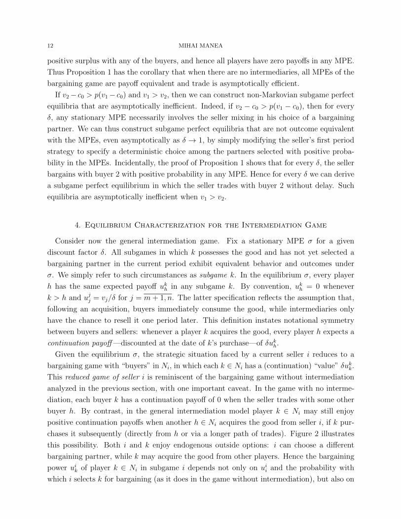
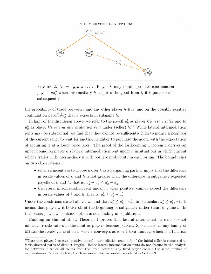
chases it subsequently (directly from h or via a longer path of trades). Figure 2 illustrates
this possibility. Both i and k enjoy endogenous outside options: i can choose a different
bargaining partner, while k may acquire the good from other players. Hence the bargaining
power uik of player k ∈ Ni in subgame i depends not only on uii and the probability with
which i selects k for bargaining (as it does in the game without intermediation), but also on
INTERMEDIATION IN NETWORKS 13
ci uii =?
δugg
δukk
δuhh
δuhk
Figure 2. Ni = {g, h, k, . . .}. Player k may obtain positive continuation
payoffs δuhk when intermediary h acquires the good from i, if k purchases it
subsequently.
the probability of trade between i and any other player h ∈ Ni and on the possibly positive
continuation payoff δuhk that k expects in subgame h.
In light of the discussion above, we refer to the payoff ukk as player k’s resale value and to
uhk as player k’s lateral intermediation rent under (seller) h.10 While lateral intermediation
rents may be substantial, we find that they cannot be sufficiently high to induce a neighbor
of the current seller to wait for another neighbor to purchase the good, with the expectation
of acquiring it at a lower price later. The proof of the forthcoming Theorem 1 derives an
upper bound on player k’s lateral intermediation rent under h in situations in which current
seller i trades with intermediary h with positive probability in equilibrium. The bound relies
on two observations:
• seller i’s incentives to choose h over k as a bargaining partner imply that the difference
in resale values of k and h is not greater than the difference in subgame i expected
payoffs of k and h, that is, ukk − uhh ≤ uik − uih;• k’s lateral intermediation rent under h, when positive, cannot exceed the difference
in resale values of k and h, that is, uhk ≤ ukk − uhh.
Under the conditions stated above, we find that uhk ≤ uik− uih. In particular, uhk ≤ uik, which
means that player k is better off at the beginning of subgame i rather than subgame h. In
this sense, player k’s outside option is not binding in equilibrium.
Building on this intuition, Theorem 1 proves that lateral intermediation rents do not
influence resale values in the limit as players become patient. Specifically, in any family of
MPEs, the resale value of each seller i converges as δ → 1 to a limit ri, which is a function
10Note that player k receives positive lateral intermediation rents only if the initial seller is connected tok via directed paths of distinct lengths. Hence lateral intermediation rents do not feature in the analysisfor networks in which all routes from the initial seller to any fixed player contain the same number ofintermediaries. A special class of such networks—tier networks—is defined in Section 9.
14 MIHAI MANEA
only of the limit resale values (rk)k∈Niof i’s neighbors. In the limit, seller i’s bargaining
power in the reduced game is derived as if the players in Ni were buyers with valuations
(rk)k∈Niin the game without intermediation. However, Remark 5 below shows that, due to
lateral intermediation rents, the current seller does not necessarily trade with the highest
resale value partner almost surely in the limit. In other words, the payoff formulae from
Proposition 1 extend to the general intermediation model (see also Remark 4), but the
structure of agreements does not.11
Theorem 1. For any family of stationary MPEs, resale values converge as δ → 1 to a vector
(ri)i∈N , which is determined recursively as follows
• rj = vj for j = m+ 1, . . . , n
• ri = max(p(rINi− ci), rII
Ni− ci, 0) for i = m,m−1, . . . , 0, where rI
Niand rII
Nidenote the
first and the second highest order statistics of the collection (rk)k∈Ni, respectively.12
The proof appears in the Appendix. We sketch the main steps here. We proceed by
backward induction on i, for i = n, n − 1, . . . , 0. To outline the inductive step for seller i,
fix a discount factor δ and a corresponding MPE σ with payoffs (ukh)k,h∈N . Assume that
the current seller i can generate positive gains by trading with one of his neighbors, i.e.,
δmaxk∈Niukk > ci. Under this assumption, we argue that if i selects k ∈ Ni as a bargaining
partner under σ, then the two players trade with probability 1. The equilibrium prices
offered by i and k are δukk − δuik and δuii + ci, respectively.
Let πk denote the probability that seller i selects player k for bargaining in subgame i
under σ. For all k ∈ Ni, we obtain the following equilibrium constraints,
uii ≥ p(δukk − ci − δuik) + (1− p)δuii, with equality if πk > 0;(4.1)
uik = πk(pδuik + (1− p)(δukk − ci − δuii)
)+
∑h∈Ni\{k}
πhδuhk.(4.2)
For example, the right-hand side of (4.2) reflects the following equilibrium properties. Seller
i trades with player k with probability πk. At the time of purchase, the good is worth a
discounted resale value of δukk to k. If πk > 0, seller i asks for a price of δukk − δuik from k,
while player k offers a price of δuii + ci to i, with respective conditional probabilities p and
1− p. Furthermore, seller i trades with neighbor h 6= k with probability πh, in which event
k enjoys a discounted lateral intermediation rent of δuhk.
11Whether the conclusion of Proposition 1 regarding outcome equivalence of MPEs generalizes to the in-termediation game is an open question. However, this technical puzzle does not restrict the scope of ouranalysis since we focus on limit equilibrium outcomes as players become patient and Theorem 1 establishesthat all MPEs generate identical limit resale values. In particular, the initial seller obtains the same limitprofit in all MPEs.12If |Ni| = 1, then rIINi
can be defined to be any non-positive number.
INTERMEDIATION IN NETWORKS 15
Consider now a family of MPEs for δ ∈ (0, 1) with payoffs (ukh)k,h∈N (the dependence of
these variables on δ is suppressed for notational convenience). The main difficulties arise
when sup{δ|δmaxk∈Niukk ≤ ci} < 1, so that bargaining does not break down for high δ.
In this case, we have that rINi≥ ci. It suffices to prove that lim infδ→1 u
ii ≥ max(p(rINi
−ci), r
IINi− ci) and lim supδ→1 u
ii ≤ max(p(rINi
− ci), rIINi− ci).
The more delicate part of the argument shows that lim infδ→1 uii ≥ p(rINi
− ci). Fix
k1 ∈ arg maxk∈Niukk (k1 is a function of δ). For high δ (such that δuk
1
k1 > ci), uik1 solves
equation (4.2) with k = k1. For all h ∈ Ni with πh > 0, the lateral intermediation rent of
player k1 under h satisfies uhk1 ≤ uik1 , as argued in the preamble of Theorem 1. Then (4.2)
implies that
uik1 ≤ pδuik1 + (1− p)(δuk1
k1 − ci − δuii).
Now substitute this bound on uik1 in the incentive constraint (4.1) for k = k1. After algebraic
manipulation, we obtain uii ≥ p(δuk1
k1 − ci). The induction hypothesis implies that uk1
k1
converges as δ → 1 to rINi. Therefore, lim infδ→1 u
ii ≥ p(rINi
− ci).To show that lim infδ→1 u
ii ≥ rIINi
− ci, note that the incentive constraint (4.1) leads to
lim infδ→1
(uii + uik1
)≥ lim
δ→1uk
1
k1 − ci = rINi− ci.
A careful accounting of payoffs (Lemma 2 in the Appendix) in subgame i establishes that
lim supδ→1
(uii +
∑k∈Ni
uik
)≤ rINi
− ci.
Then for any player k2 ∈ arg maxk∈Ni\{k1} ukk, we have limδ→1 u
ik2 = 0. The incentive con-
straint (4.1) with k = k2 leads to uii(1−(1−p)δ)+pδuik2 ≥ p(δuk2
k2−ci). Since limδ→1 uk2
k2 = rIINi
by the induction hypothesis, we obtain lim infδ→1 uii ≥ rIINi
− ci.We prove that lim supδ→1 u
ii ≤ max(p(rINi
− ci), rIINi− ci) by contradiction. If the claim
is false, then there exists a sequence of discount factors converging to 1 along which (1) uiiconverges to a limit greater than max(p(rINi
− ci), rIINi− ci), and (2) seller i either (i) trades
exclusively with a (fixed) player k or (ii) trades with positive probability with two (fixed)
players k and h such that ukk ≥ uhh. In case (i), the payoff equations lead to uii = p(δukk − ci).Then the induction hypothesis implies that the limit of uii along the sequence is p(rk− ci) ≤p(rINi
− ci).In case (ii), (4.1) implies that uii(1 − (1 − p)δ) ≤ p(δuhh − ci). Note that ukk ≥ uhh, along
with the induction hypothesis, leads to rk = limδ→1 ukk ≥ limδ→1 u
hh = rh. Hence the limit
of uii along the sequence does not exceed rh − ci ≤ rIINi− ci. In either case, we reach a
contradiction.
Remark 4. The proof shows that the characterization of buyer payoffs from Proposition 1
also extends to the intermediation game. The intermediation rent uik extracted by player
16 MIHAI MANEA
c0
c1
v2 v3
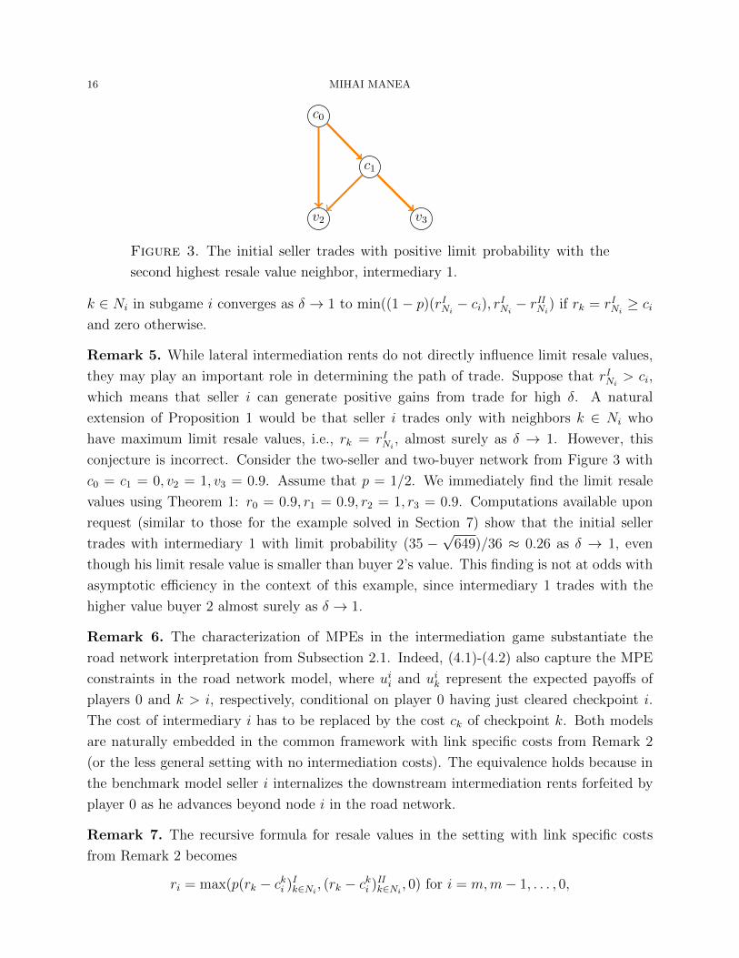
Figure 3. The initial seller trades with positive limit probability with the
second highest resale value neighbor, intermediary 1.
k ∈ Ni in subgame i converges as δ → 1 to min((1− p)(rINi− ci), rINi
− rIINi) if rk = rINi
≥ ci
and zero otherwise.
Remark 5. While lateral intermediation rents do not directly influence limit resale values,
they may play an important role in determining the path of trade. Suppose that rINi> ci,
which means that seller i can generate positive gains from trade for high δ. A natural
extension of Proposition 1 would be that seller i trades only with neighbors k ∈ Ni who
have maximum limit resale values, i.e., rk = rINi, almost surely as δ → 1. However, this
conjecture is incorrect. Consider the two-seller and two-buyer network from Figure 3 with
c0 = c1 = 0, v2 = 1, v3 = 0.9. Assume that p = 1/2. We immediately find the limit resale
values using Theorem 1: r0 = 0.9, r1 = 0.9, r2 = 1, r3 = 0.9. Computations available upon
request (similar to those for the example solved in Section 7) show that the initial seller
trades with intermediary 1 with limit probability (35 −√
649)/36 ≈ 0.26 as δ → 1, even
though his limit resale value is smaller than buyer 2’s value. This finding is not at odds with
asymptotic efficiency in the context of this example, since intermediary 1 trades with the
higher value buyer 2 almost surely as δ → 1.
Remark 6. The characterization of MPEs in the intermediation game substantiate the
road network interpretation from Subsection 2.1. Indeed, (4.1)-(4.2) also capture the MPE
constraints in the road network model, where uii and uik represent the expected payoffs of
players 0 and k > i, respectively, conditional on player 0 having just cleared checkpoint i.
The cost of intermediary i has to be replaced by the cost ck of checkpoint k. Both models
are naturally embedded in the common framework with link specific costs from Remark 2
(or the less general setting with no intermediation costs). The equivalence holds because in
the benchmark model seller i internalizes the downstream intermediation rents forfeited by
player 0 as he advances beyond node i in the road network.
Remark 7. The recursive formula for resale values in the setting with link specific costs
from Remark 2 becomes
ri = max(p(rk − cki )Ik∈Ni, (rk − cki )IIk∈Ni
, 0) for i = m,m− 1, . . . , 0,
INTERMEDIATION IN NETWORKS 17
where (rk − cki )Ik∈Niand (rk − cki )IIk∈Ni
denote the first and the second highest order statistics
of the collection (rk − cki )k∈Ni, respectively. To extend the proofs of Theorem 1 and the
supporting Lemma 2 to this more general setting, we need to assume that direct connections
are not more costly than indirect ones. Formally, for any link (i, k) and all directed paths
i = i0, i1, . . . , is = k (is ∈ Nis−1 for all s = 1, s) connecting i to k, it must be that
cki ≤s−1∑s=0
cis+1
is.
Note that the condition above is satisfied whenever cki depends exclusively on i—as in our
benchmark model—or on k—as in the road network version.
4.1. Relationship to double marginalization. Consider a line network (Ni = {i + 1}for i = 0, n− 1) with a single buyer (player n) and no intermediation costs (ci = 0 for
i = 0, n− 1). The formula for limit resale values from Theorem 1 implies that ri = pn−ivn
for i = 0, n− 1. This conclusion is reminiscent of double marginalization (Spengler 1950).
However, there does not seem to be a deep theoretical connection between intermediation
in networks and multiple marginalization in a chain of monopolies. The two models capture
distinct strategic situations. In the classic double marginalization paradigm, upstream mo-
nopolists set prices for downstream firms, which implicitly determine the amount of trade
in each transaction. Downstream firms have no bargaining power. By contrast, in the line
network application of our intermediation game, downstream neighbors derive bargaining
power from the opportunity of making offers to upstream sellers, which arises with prob-
ability 1 − p at every date. Every link represents a bilateral monopoly. Moreover, since
our environment presumes that a single unit of the indivisible good is available, there is no
discretion over the quantity traded in each agreement. It is worth emphasizing here that
our focus is on understanding how competition among trading paths shapes the outcomes
of intermediation. Since competition is entirely absent in line networks, any relationship to
double marginalization is peripheral to our main contribution.
4.2. Equilibrium existence. Using the properties of MPEs uncovered by the analysis
above, we establish the existence of an equilibrium.
Proposition 2. A stationary MPE exists in the intermediation game.
5. Layers of Intermediation Power
This section investigates how an intermediary’s position in the network affects his resale
value. In order to focus exclusively on network asymmetries, suppose momentarily that
sellers have zero costs and buyers have a common value v (or that there is a single buyer,
i.e., m = n−1). Since no resale value can exceed v, Theorem 1 implies that any seller linked
18 MIHAI MANEA
to two (or more) buyers has a limit resale value of v. Then any seller linked to at least two
of the latter players also secures a payoff of v, acting as a monopolist for players with limit
continuation payoffs of v. More generally, any trader linked to two players with a resale value
of v also obtains a limit price of v. We continue to identify players with a resale value v in
this fashion until we reach a stage where no remaining seller is linked to two others known
to have resale value v.
Using Theorem 1 again, we can show that each remaining trader linked to one value v
player has resale value pv. We can then identify additional traders who command a resale
price of pv due to competition between multiple neighbors with resale value pv, and so on.
We are thus led to decompose the network into a sequence of layers of intermediation
power, (L`)`≥0, which characterizes every player’s resale value. The recursive construction
proceeds as follows. First all buyers are enlisted in layer 0. In general, for ` ≥ 1, having
defined layers 0 through `− 1, the first players to join layer ` are those outside⋃`′<` L`′ who
are linked to a node in L`−1. For every ` ≥ 0, given the initial membership of layer `, new
traders outside⋃`′<` L`′ with at least two links to established members of layer ` are added
to the layer. We continue expanding layer ` until no remaining seller is linked to two of its
formerly recognized members. All players joining layer ` through this sequential procedure
constitute L`.13 The algorithm terminates when every player is uniquely assigned to a layer,⋃`′≤` L`′ = N . For an illustration, in the network example from Figure 1 the algorithm
produces the layers L0 = {5, 9, 10},L1 = {0, 1, 3, 4, 6, 7, 8},L2 = {2}.The definition of each layer is obviously independent of the order in which players join the
layer. In fact, an equivalent description of the layer decomposition proceeds as follows. L0
is the largest set (with respect to inclusion) M ⊂ N , which contains all buyers, such that
every seller in M has two (or more) out-links to other players in M . For ` ≥ 1, L` is the
largest set M ⊂ N \(⋃
`′<` L`′)
with the property that every node in M has out-links to
either (exactly) one node in L`−1 or (at least) two nodes in M .
The informal arguments above suggest that if sellers have zero costs and buyers have the
same value v, then all players from layer ` have a resale value of p`v. The next result proves a
generalization of this claim for arbitrary cost structures. It provides lower and upper bounds
anchored at p`v for the resale values of layer ` players. The precision of the bounds for player
i ∈ L` depends on the sum of costs of sellers k ≥ i from layers `′ ≤ ` weighted by p`−`′. In
particular, the bounds become tight as intermediation costs vanish. Thus the decomposition
of the network into layers captures intermediation power.
13Note that layer ` has an analogous topology to layer 0, if we recast the initial members of layer ` as buyers.
INTERMEDIATION IN NETWORKS 19
c0
c1
c3
c6
c2
c4
c7
c10
c5
c8
c11
c13
c9
c12
c14
v15
c0
c1
c3
c6
c2
c4
c7
c10
c5
c8
c11
c13
c9
c12
c14
v15
Figure 4. A square lattice and a triangular grid
c0
c2
c4
c6
c8
v9
c7
c5
c3
c1
Figure 5. An enhanced circle network
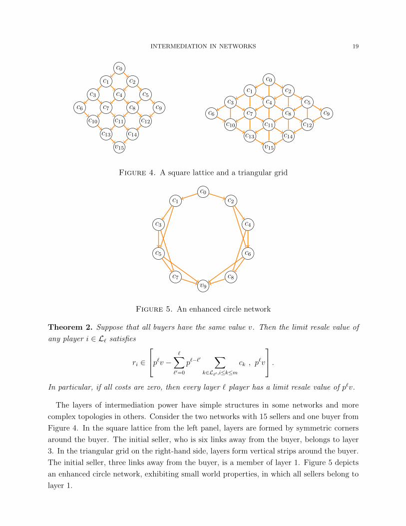
Theorem 2. Suppose that all buyers have the same value v. Then the limit resale value of
any player i ∈ L` satisfies
ri ∈
p`v − ∑`′=0
p`−`′ ∑k∈L`′ ,i≤k≤m
ck , p`v
.In particular, if all costs are zero, then every layer ` player has a limit resale value of p`v.
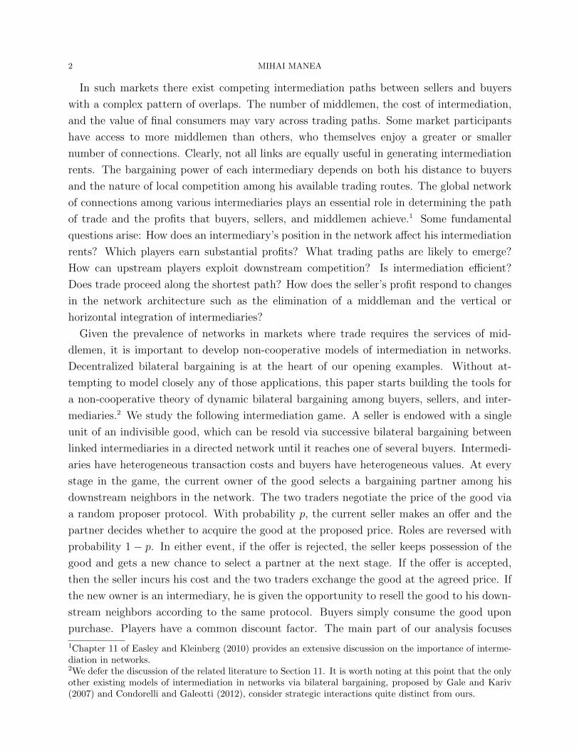
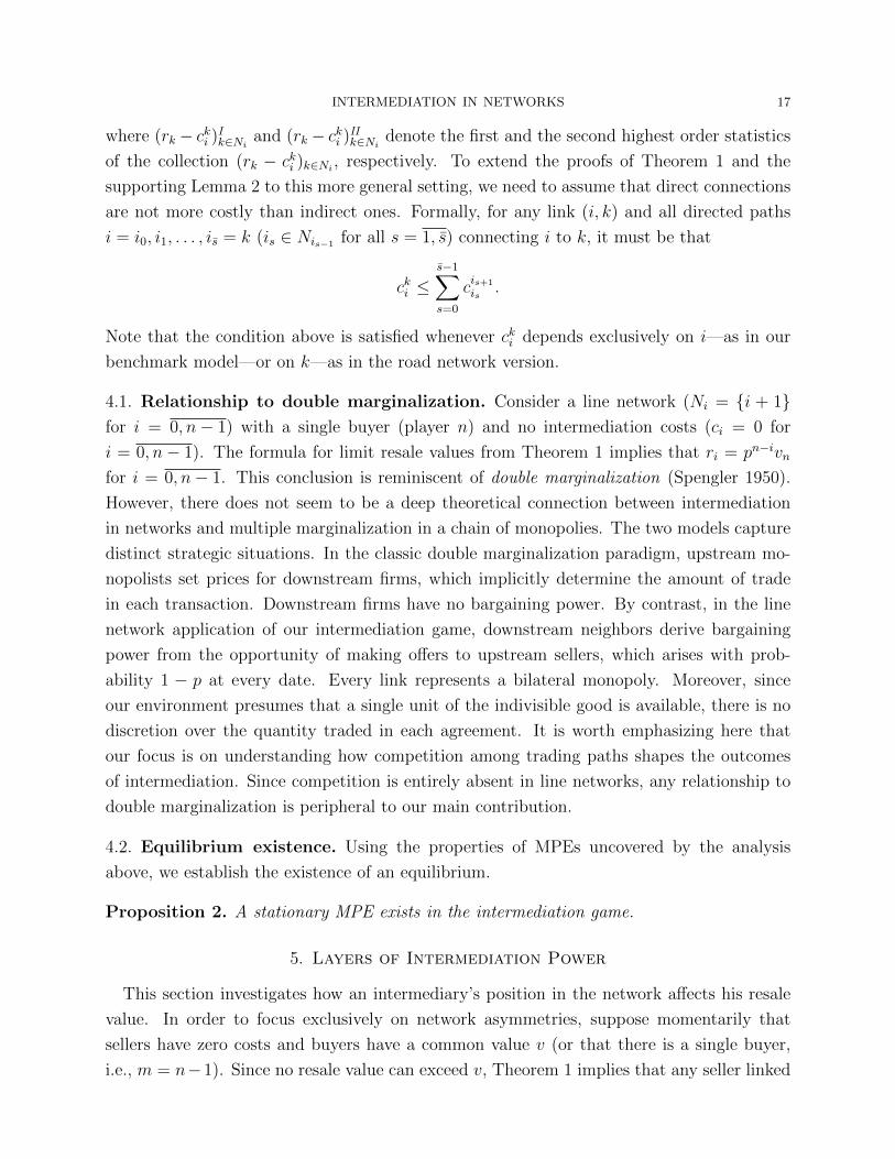
The layers of intermediation power have simple structures in some networks and more
complex topologies in others. Consider the two networks with 15 sellers and one buyer from
Figure 4. In the square lattice from the left panel, layers are formed by symmetric corners
around the buyer. The initial seller, who is six links away from the buyer, belongs to layer
3. In the triangular grid on the right-hand side, layers form vertical strips around the buyer.
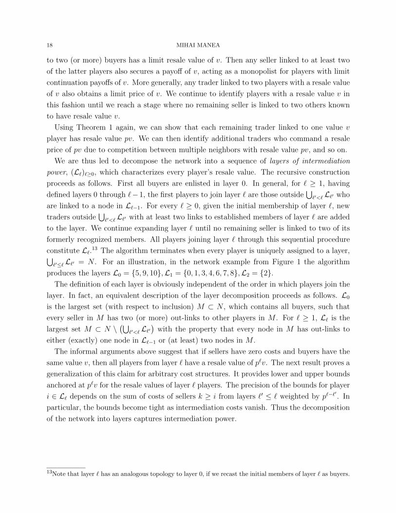
The initial seller, three links away from the buyer, is a member of layer 1. Figure 5 depicts
an enhanced circle network, exhibiting small world properties, in which all sellers belong to
layer 1.
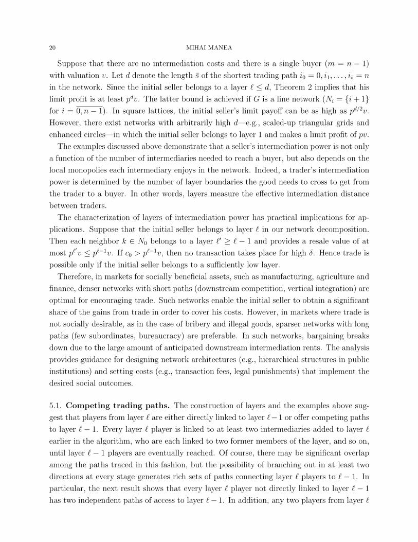
20 MIHAI MANEA
Suppose that there are no intermediation costs and there is a single buyer (m = n − 1)
with valuation v. Let d denote the length s of the shortest trading path i0 = 0, i1, . . . , is = n
in the network. Since the initial seller belongs to a layer ` ≤ d, Theorem 2 implies that his
limit profit is at least pdv. The latter bound is achieved if G is a line network (Ni = {i+ 1}for i = 0, n− 1). In square lattices, the initial seller’s limit payoff can be as high as pd/2v.
However, there exist networks with arbitrarily high d—e.g., scaled-up triangular grids and
enhanced circles—in which the initial seller belongs to layer 1 and makes a limit profit of pv.
The examples discussed above demonstrate that a seller’s intermediation power is not only
a function of the number of intermediaries needed to reach a buyer, but also depends on the
local monopolies each intermediary enjoys in the network. Indeed, a trader’s intermediation
power is determined by the number of layer boundaries the good needs to cross to get from
the trader to a buyer. In other words, layers measure the effective intermediation distance
between traders.
The characterization of layers of intermediation power has practical implications for ap-
plications. Suppose that the initial seller belongs to layer ` in our network decomposition.
Then each neighbor k ∈ N0 belongs to a layer `′ ≥ ` − 1 and provides a resale value of at
most p`′v ≤ p`−1v. If c0 > p`−1v, then no transaction takes place for high δ. Hence trade is
possible only if the initial seller belongs to a sufficiently low layer.
Therefore, in markets for socially beneficial assets, such as manufacturing, agriculture and
finance, denser networks with short paths (downstream competition, vertical integration) are
optimal for encouraging trade. Such networks enable the initial seller to obtain a significant
share of the gains from trade in order to cover his costs. However, in markets where trade is
not socially desirable, as in the case of bribery and illegal goods, sparser networks with long
paths (few subordinates, bureaucracy) are preferable. In such networks, bargaining breaks
down due to the large amount of anticipated downstream intermediation rents. The analysis
provides guidance for designing network architectures (e.g., hierarchical structures in public
institutions) and setting costs (e.g., transaction fees, legal punishments) that implement the
desired social outcomes.
5.1. Competing trading paths. The construction of layers and the examples above sug-
gest that players from layer ` are either directly linked to layer `−1 or offer competing paths
to layer `− 1. Every layer ` player is linked to at least two intermediaries added to layer `
earlier in the algorithm, who are each linked to two former members of the layer, and so on,
until layer `− 1 players are eventually reached. Of course, there may be significant overlap
among the paths traced in this fashion, but the possibility of branching out in at least two
directions at every stage generates rich sets of paths connecting layer ` players to `− 1. In
particular, the next result shows that every layer ` player not directly linked to layer ` − 1
has two independent paths of access to layer `− 1. In addition, any two players from layer `
INTERMEDIATION IN NETWORKS 21
can reach layer `− 1 via disjoint paths of layer ` intermediaries. In other words, every pair
of intermediaries from layer ` can pass the good down to layer `− 1 without relying on each
other or on any common layer ` intermediaries.
Proposition 3. Every player from layer ` ≥ 1 has either a direct link to layer `− 1 or two
non-overlapping paths of layer ` intermediaries connecting him to (possibly the same) layer
` − 1 players. Moreover, any pair of distinct layer ` ≥ 1 players can reach some (possibly
identical) layer `− 1 players via disjoint paths of layer ` intermediaries.
It is possible to prove the following version of the result for layer 0. Every seller from layer
0 is connected to two different buyers via non-overlapping paths of layer 0 intermediaries.
Furthermore, any pair of sellers from layer 0 can reach distinct buyers using disjoint paths
of layer 0 intermediaries.
6. Intermediation Inefficiencies
In contrast to the bargaining model with no intermediaries analyzed in Section 3, in-
termediation may create trade inefficiencies. There are two distinct sources of asymp-
totic inefficiency. One source resides in hold-up problems induced by the bilateral na-
ture of intermediation combined with weak downstream competition. Consider a subgame
in which a current seller i creates positive net profit by trading with the highest resale
value neighbor, but cannot capture the entire surplus available in the transaction, that is,
ri = max(p(rINi− ci), r
IINi− ci, 0) < rINi
− ci. Then rINi> max(rIINi
, ci) and the (unique)
player with the highest resale value secures positive rents of min((1− p)(rINi− ci), rINi
− rIINi)
(Remark 4). The rent amount is independent of the history of transactions; in particular,
the payment i made to procure the good is sunk. Such rents are anticipated by upstream
traders and diminish the gains they share.14 In some cases, the dissipation of surplus is so
extreme that trade becomes unprofitable even though some intermediation chains generate
positive total surplus.
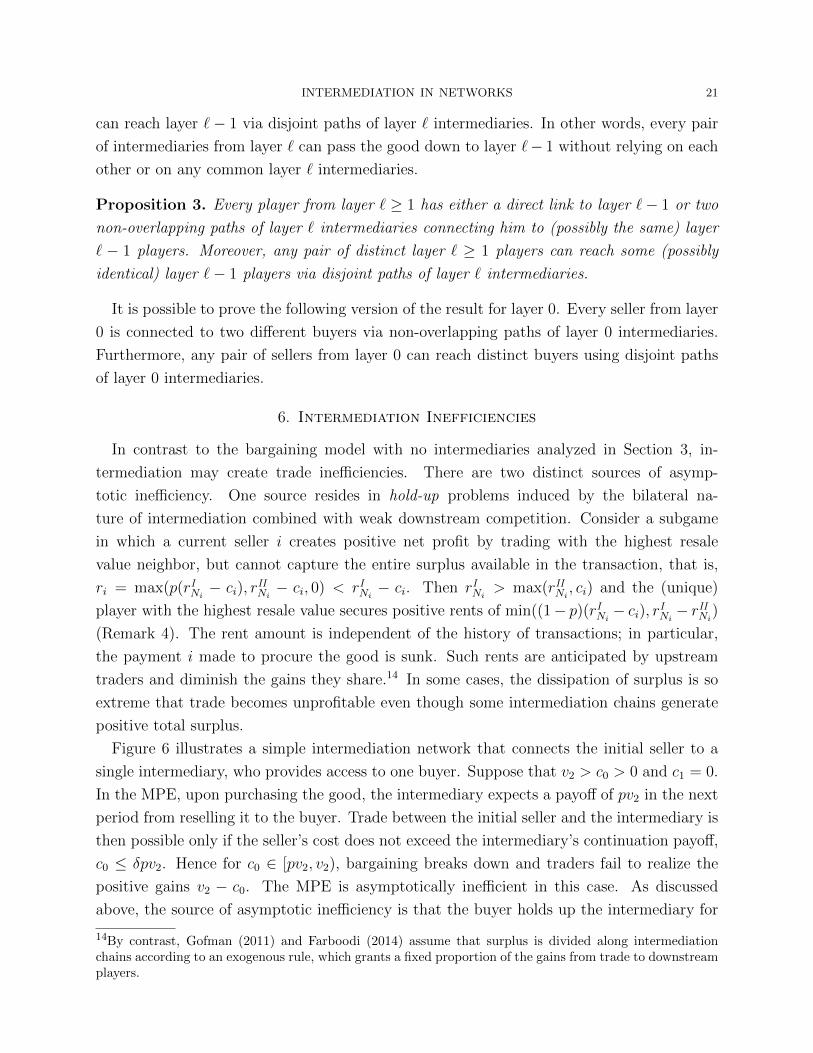
Figure 6 illustrates a simple intermediation network that connects the initial seller to a
single intermediary, who provides access to one buyer. Suppose that v2 > c0 > 0 and c1 = 0.
In the MPE, upon purchasing the good, the intermediary expects a payoff of pv2 in the next
period from reselling it to the buyer. Trade between the initial seller and the intermediary is
then possible only if the seller’s cost does not exceed the intermediary’s continuation payoff,
c0 ≤ δpv2. Hence for c0 ∈ [pv2, v2), bargaining breaks down and traders fail to realize the
positive gains v2 − c0. The MPE is asymptotically inefficient in this case. As discussed
above, the source of asymptotic inefficiency is that the buyer holds up the intermediary for
14By contrast, Gofman (2011) and Farboodi (2014) assume that surplus is divided along intermediationchains according to an exogenous rule, which grants a fixed proportion of the gains from trade to downstreamplayers.

22 MIHAI MANEA
c0
c1
v2
Figure 6. Hold-up inefficiencies
a profit of (1− p)v2. Then at the initial stage the seller and the intermediary bargain over a
reduced limit surplus of pv2 − c0, rather than the total amount of v2 − c0.15 The conclusion
of this example can be immediately extended to show that in any setting with at least one
intermediary (m ≥ 1) there exist configurations of intermediation costs and buyer values
such that trade is asymptotically inefficient.
Proposition 4. For any linking structure (Ni)i=0,m with m ≥ 1 intermediaries there exist
cost and value configurations ((ci)i=0,m, (vj)j=m+1,n) such that any family of MPEs induced
by the network (N, (Ni)i=0,m, (ci)i=0,m, (vj)j=m+1,n) is asymptotically inefficient.
For a sketch of the proof, note that for any linking structure (Ni)i=0,m with m ≥ 1 there
must be a trading path i0 = 0, i1 = 1, . . . , is with s ≥ 2. If we set c0 ∈ (ps−1, 1), cis = 0
for s = 1, s− 1, vis = 1, the costs of all remaining intermediaries to 1, and the values of all
buyers different from is to 0, then no trade takes place in equilibrium even though the path
(is)s=0,s generates positive surplus.
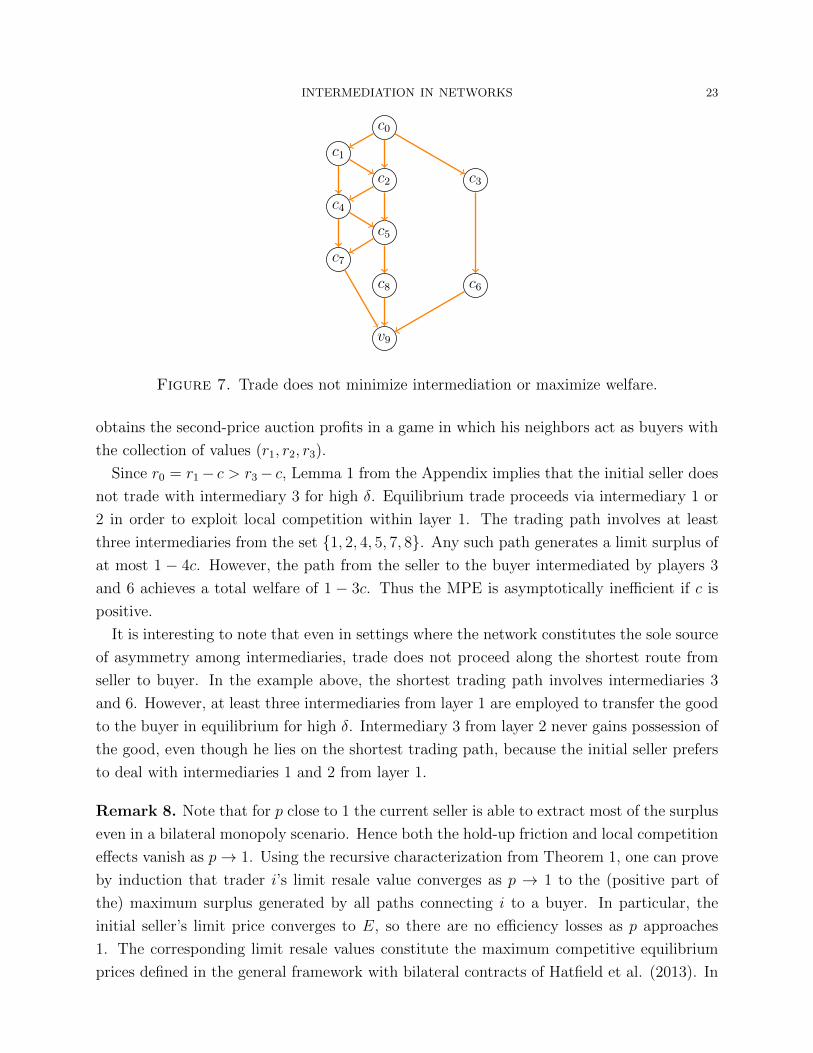
Another source of inefficiency lies in sellers’ incentives to exploit local competition, which
are not aligned with global welfare maximization. Consider the network from Figure 7, in
which the buyer value v9 is normalized to 1 and sellers are assumed to have a common cost
c ∈[0,min
(p(1− p)4− p2
,p(1− p)
5− 3p− p2
)).
In this network, the layer decomposition algorithm leads to
L0 = {9},L1 = {0, 1, 2, 4, 5, 6, 7, 8},L2 = {3}.
Resale values are easily computed from Theorem 1. In particular, we find that r0 = p −(5 + p)c, r1 = p − (4 + p)c, r2 = p − (3 + p)c, and r3 = p2 − p(1 + p)c. For the range of c
considered, we have r2 ≥ r1 > r3 and r0 = r1 − c > p(r2 − c) > 0. Hence the initial seller
15Blanchard and Kremer (1997) and Wong and Wright (2011) discuss similar hold-up problems in linenetworks.
INTERMEDIATION IN NETWORKS 23
c0
c1
c4
c7
c2
c5
c8
c3
c6
v9
Figure 7. Trade does not minimize intermediation or maximize welfare.
obtains the second-price auction profits in a game in which his neighbors act as buyers with
the collection of values (r1, r2, r3).
Since r0 = r1− c > r3− c, Lemma 1 from the Appendix implies that the initial seller does
not trade with intermediary 3 for high δ. Equilibrium trade proceeds via intermediary 1 or
2 in order to exploit local competition within layer 1. The trading path involves at least
three intermediaries from the set {1, 2, 4, 5, 7, 8}. Any such path generates a limit surplus of
at most 1 − 4c. However, the path from the seller to the buyer intermediated by players 3
and 6 achieves a total welfare of 1 − 3c. Thus the MPE is asymptotically inefficient if c is
positive.
It is interesting to note that even in settings where the network constitutes the sole source
of asymmetry among intermediaries, trade does not proceed along the shortest route from
seller to buyer. In the example above, the shortest trading path involves intermediaries 3
and 6. However, at least three intermediaries from layer 1 are employed to transfer the good
to the buyer in equilibrium for high δ. Intermediary 3 from layer 2 never gains possession of
the good, even though he lies on the shortest trading path, because the initial seller prefers
to deal with intermediaries 1 and 2 from layer 1.
Remark 8. Note that for p close to 1 the current seller is able to extract most of the surplus
even in a bilateral monopoly scenario. Hence both the hold-up friction and local competition
effects vanish as p→ 1. Using the recursive characterization from Theorem 1, one can prove
by induction that trader i’s limit resale value converges as p → 1 to the (positive part of
the) maximum surplus generated by all paths connecting i to a buyer. In particular, the
initial seller’s limit price converges to E, so there are no efficiency losses as p approaches
1. The corresponding limit resale values constitute the maximum competitive equilibrium
prices defined in the general framework with bilateral contracts of Hatfield et al. (2013). In
24 MIHAI MANEA
c0
c1
c2 c3
v4
q
1-q
0.1 0.2 0.3 0.4 0.5 0.6 0.7 0.8 0.9 1 p
0.1
0.2
0.3
0.4
0.5
0.6
0.7
0.8
0.9
1lim∆®1q
Figure 8. Asymmetric trading paths within layers
contrast to the findings of this section, competitive equilibria in the latter model are always
efficient. We elaborate on the modeling assumptions that underlie the divergent predictions
in the literature review (Section 11).
7. Positive Profits
It is important to determine which intermediaries make significant profits. This question
is challenging because the path of trade is not necessarily deterministic in equilibrium. We
reinstate the zero costs and homogeneous values assumptions of Section 5. Although traders
from the same layer have identical limit resale values, it turns out that MPE trading paths
may treat such traders asymmetrically, even in the limit as players become patient. Indeed,
as the next example illustrates, two trading partners with vanishing differences in resale
values and lateral intermediation rents may acquire the good from the seller with unequal
positive limit probabilities.
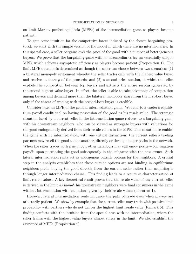
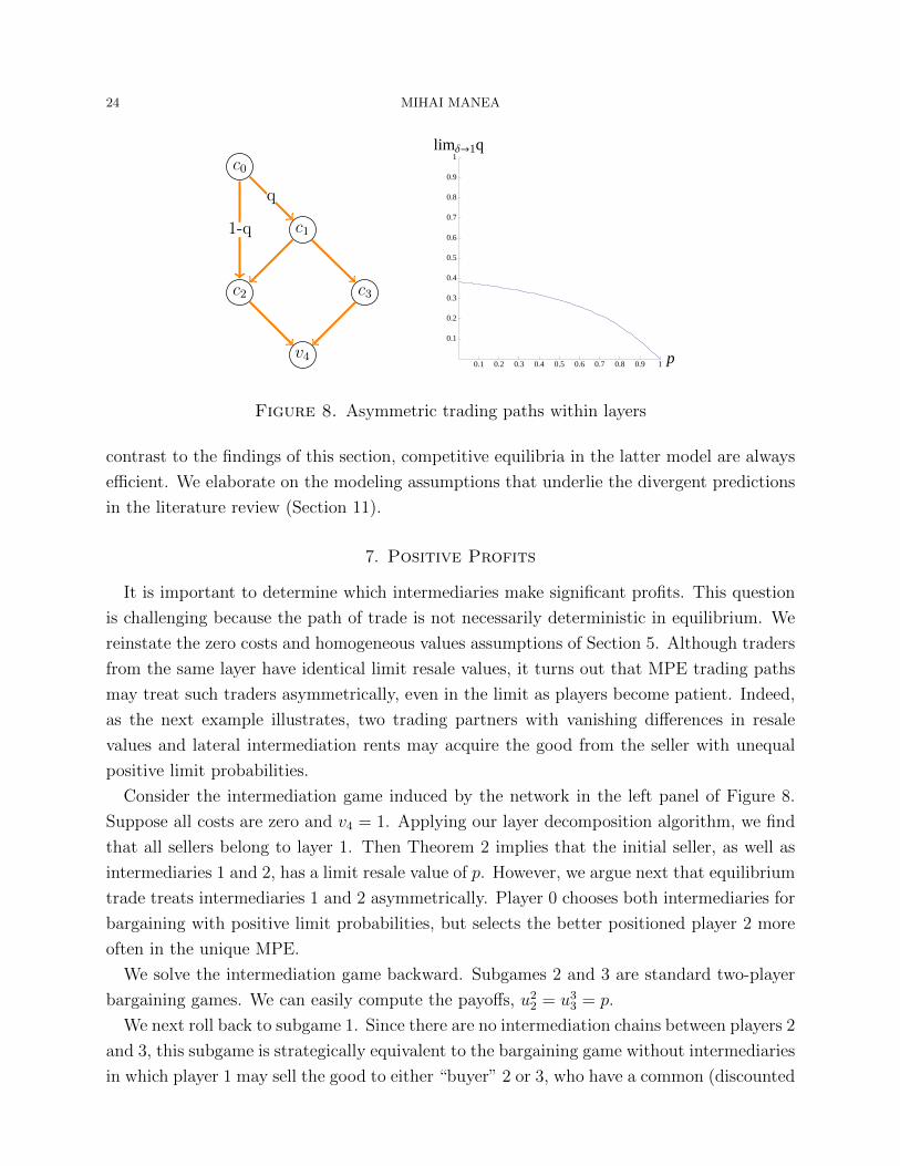
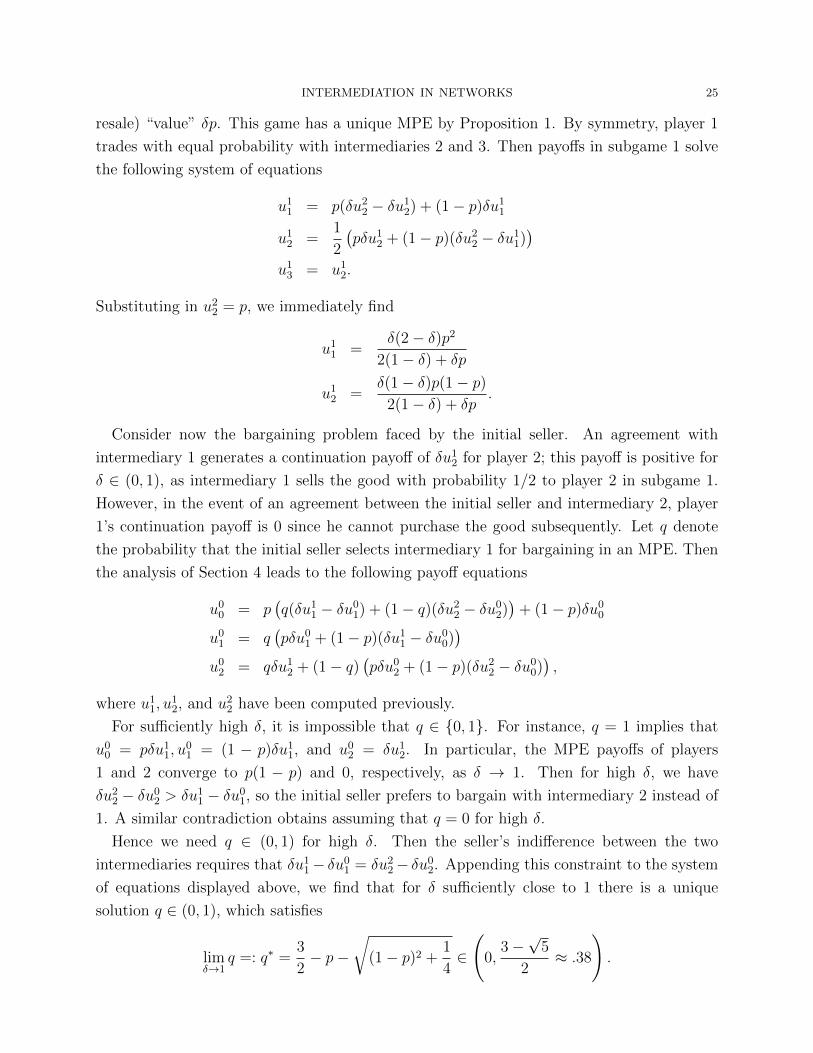
Consider the intermediation game induced by the network in the left panel of Figure 8.
Suppose all costs are zero and v4 = 1. Applying our layer decomposition algorithm, we find
that all sellers belong to layer 1. Then Theorem 2 implies that the initial seller, as well as
intermediaries 1 and 2, has a limit resale value of p. However, we argue next that equilibrium
trade treats intermediaries 1 and 2 asymmetrically. Player 0 chooses both intermediaries for
bargaining with positive limit probabilities, but selects the better positioned player 2 more
often in the unique MPE.
We solve the intermediation game backward. Subgames 2 and 3 are standard two-player
bargaining games. We can easily compute the payoffs, u22 = u3
3 = p.
We next roll back to subgame 1. Since there are no intermediation chains between players 2
and 3, this subgame is strategically equivalent to the bargaining game without intermediaries
in which player 1 may sell the good to either “buyer” 2 or 3, who have a common (discounted
INTERMEDIATION IN NETWORKS 25
resale) “value” δp. This game has a unique MPE by Proposition 1. By symmetry, player 1
trades with equal probability with intermediaries 2 and 3. Then payoffs in subgame 1 solve
the following system of equations
u11 = p(δu2
2 − δu12) + (1− p)δu1
1
u12 =
1
2
(pδu1
2 + (1− p)(δu22 − δu1
1))
u13 = u1
2.
Substituting in u22 = p, we immediately find
u11 =
δ(2− δ)p2
2(1− δ) + δp
u12 =
δ(1− δ)p(1− p)2(1− δ) + δp
.
Consider now the bargaining problem faced by the initial seller. An agreement with
intermediary 1 generates a continuation payoff of δu12 for player 2; this payoff is positive for
δ ∈ (0, 1), as intermediary 1 sells the good with probability 1/2 to player 2 in subgame 1.
However, in the event of an agreement between the initial seller and intermediary 2, player
1’s continuation payoff is 0 since he cannot purchase the good subsequently. Let q denote
the probability that the initial seller selects intermediary 1 for bargaining in an MPE. Then
the analysis of Section 4 leads to the following payoff equations
u00 = p
(q(δu1
1 − δu01) + (1− q)(δu2
2 − δu02))
+ (1− p)δu00
u01 = q
(pδu0
1 + (1− p)(δu11 − δu0
0))
u02 = qδu1
2 + (1− q)(pδu0
2 + (1− p)(δu22 − δu0
0)),
where u11, u
12, and u2
2 have been computed previously.
For sufficiently high δ, it is impossible that q ∈ {0, 1}. For instance, q = 1 implies that
u00 = pδu1
1, u01 = (1 − p)δu1
1, and u02 = δu1
2. In particular, the MPE payoffs of players
1 and 2 converge to p(1 − p) and 0, respectively, as δ → 1. Then for high δ, we have
δu22 − δu0
2 > δu11 − δu0
1, so the initial seller prefers to bargain with intermediary 2 instead of
1. A similar contradiction obtains assuming that q = 0 for high δ.
Hence we need q ∈ (0, 1) for high δ. Then the seller’s indifference between the two
intermediaries requires that δu11− δu0
1 = δu22− δu0
2. Appending this constraint to the system
of equations displayed above, we find that for δ sufficiently close to 1 there is a unique
solution q ∈ (0, 1), which satisfies
limδ→1
q =: q∗ =3
2− p−
√(1− p)2 +
1
4∈
(0,
3−√
5
2≈ .38
).
26 MIHAI MANEA
The graph in the right panel of Figure 8 traces the relationship between the limit q∗ and the
parameter p.
The good is traded along each of the paths 0, 1, 2, 4 and 0, 1, 3, 4 with probability q/2 and
along the shorter path 0, 2, 4 with probably 1 − q. The example can be easily adapted so
that the value of q affects the distribution of profits in the network. Suppose, for instance,
that the buyer is replaced by two unit value buyers, one connected to intermediary 2 and
the other to 3. Then the limit MPE payoffs of the two buyers are (1 − p)(1 − q∗/2) and
(1− p)q∗/2, respectively.
The intricate derivation of q in the example above suggests that in general networks it is
difficult to compute the random path of trade. However, the next result shows how profits are
shared along any trading path that emerges with positive probability in equilibrium. More
specifically, it identifies the exchanges in which the new owner secures positive intermediation
rents.
Proposition 5. Suppose that sellers have zero costs and buyers have a common value v.
Then for sufficiently high δ, every layer ` player can acquire the good in equilibrium only
from traders in layers ` and ` + 1. If player k ∈ L` purchases the good from seller i with
positive probability in subgame i for a sequence of δ’s converging to 1, then player k’s limit
profit conditional on being selected by i as a trading partner is p`(1−p)v if i ∈ L`+1 and zero
if i ∈ L`.
This result establishes that players make positive limit profits only in transactions in
which they constitute a gateway to a lower layer. Hence layers delineate monopoly power
from intermediation power. Local competition is exploited in exchanges within the same
layer to extract the full amount of gains from trade, while intermediation rents need to be
surrendered in agreements across layers.
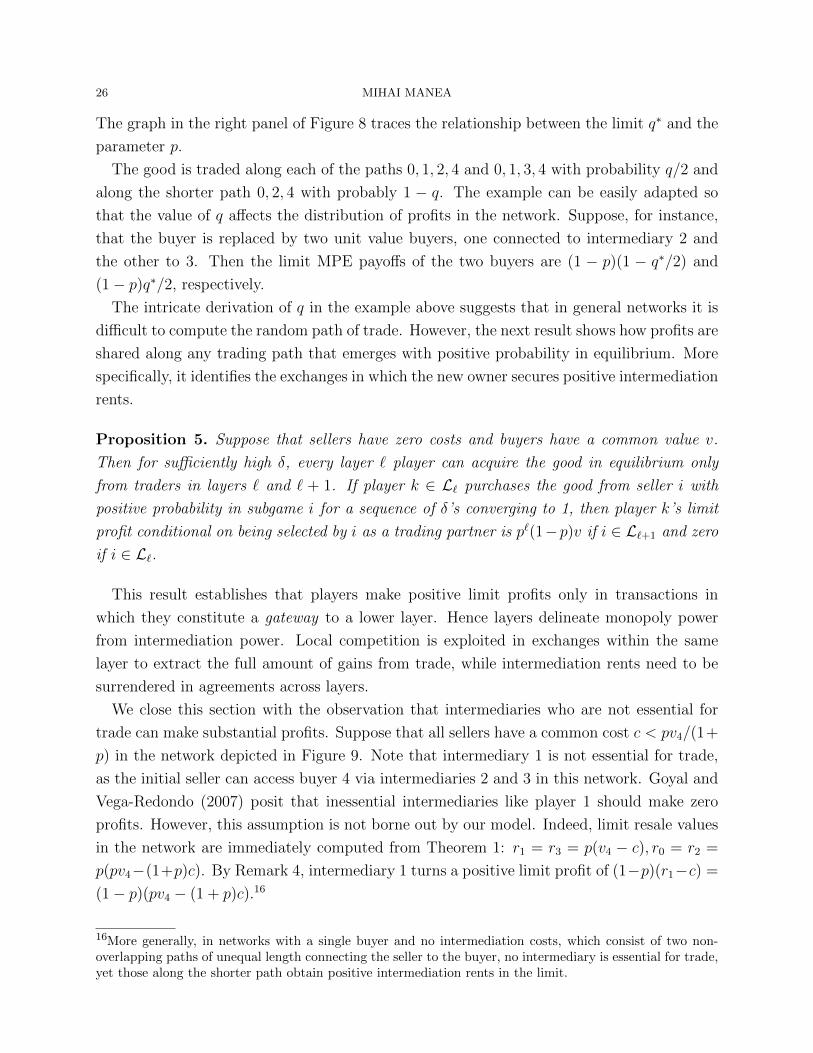
We close this section with the observation that intermediaries who are not essential for
trade can make substantial profits. Suppose that all sellers have a common cost c < pv4/(1+
p) in the network depicted in Figure 9. Note that intermediary 1 is not essential for trade,
as the initial seller can access buyer 4 via intermediaries 2 and 3 in this network. Goyal and
Vega-Redondo (2007) posit that inessential intermediaries like player 1 should make zero
profits. However, this assumption is not borne out by our model. Indeed, limit resale values
in the network are immediately computed from Theorem 1: r1 = r3 = p(v4 − c), r0 = r2 =
p(pv4−(1+p)c). By Remark 4, intermediary 1 turns a positive limit profit of (1−p)(r1−c) =
(1− p)(pv4 − (1 + p)c).16
16More generally, in networks with a single buyer and no intermediation costs, which consist of two non-overlapping paths of unequal length connecting the seller to the buyer, no intermediary is essential for trade,yet those along the shorter path obtain positive intermediation rents in the limit.
INTERMEDIATION IN NETWORKS 27
c0
c2
c3
v4
c1
Figure 9. Intermediary 1 is not essential for trade, but makes positive limit profit.
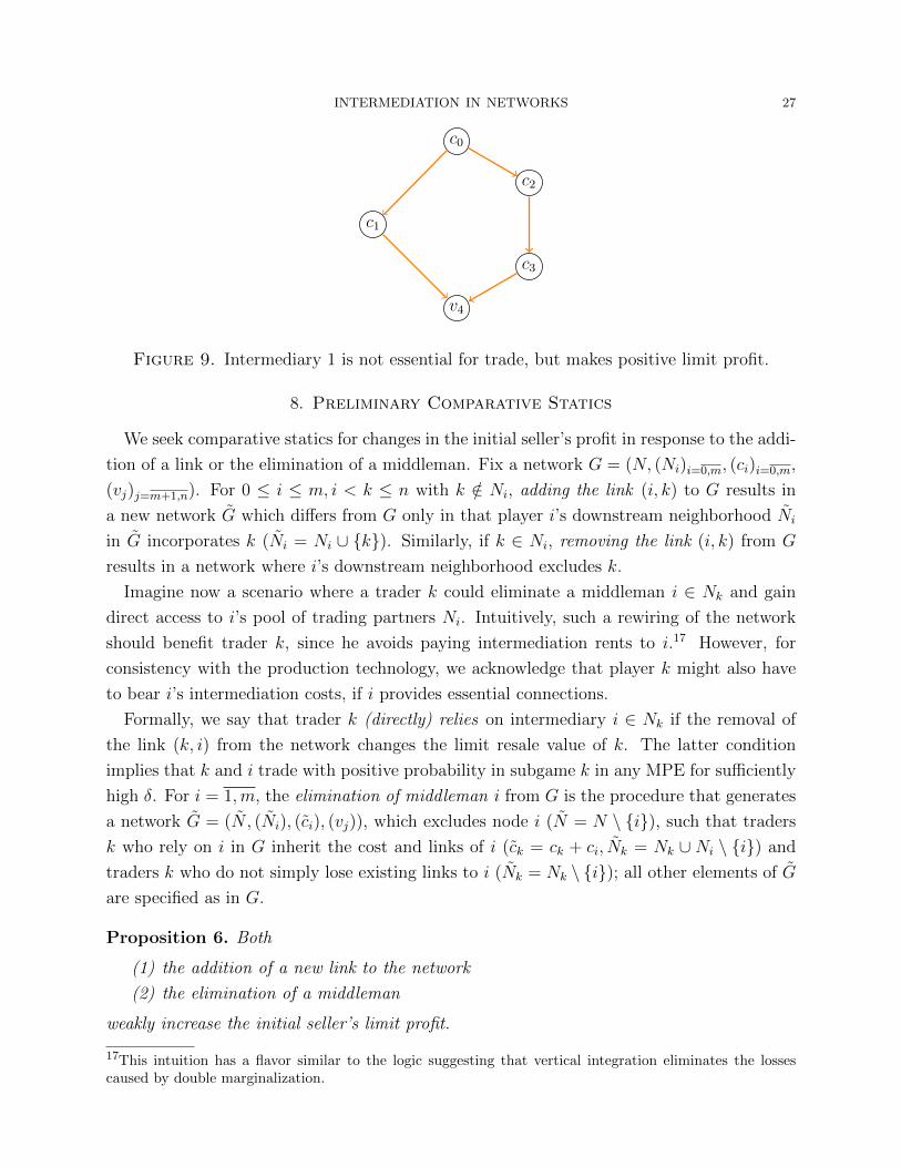
8. Preliminary Comparative Statics
We seek comparative statics for changes in the initial seller’s profit in response to the addi-
tion of a link or the elimination of a middleman. Fix a network G = (N, (Ni)i=0,m, (ci)i=0,m,
(vj)j=m+1,n). For 0 ≤ i ≤ m, i < k ≤ n with k /∈ Ni, adding the link (i, k) to G results in
a new network G which differs from G only in that player i’s downstream neighborhood Ni
in G incorporates k (Ni = Ni ∪ {k}). Similarly, if k ∈ Ni, removing the link (i, k) from G
results in a network where i’s downstream neighborhood excludes k.
Imagine now a scenario where a trader k could eliminate a middleman i ∈ Nk and gain
direct access to i’s pool of trading partners Ni. Intuitively, such a rewiring of the network
should benefit trader k, since he avoids paying intermediation rents to i.17 However, for
consistency with the production technology, we acknowledge that player k might also have
to bear i’s intermediation costs, if i provides essential connections.
Formally, we say that trader k (directly) relies on intermediary i ∈ Nk if the removal of
the link (k, i) from the network changes the limit resale value of k. The latter condition
implies that k and i trade with positive probability in subgame k in any MPE for sufficiently
high δ. For i = 1,m, the elimination of middleman i from G is the procedure that generates
a network G = (N , (Ni), (ci), (vj)), which excludes node i (N = N \ {i}), such that traders
k who rely on i in G inherit the cost and links of i (ck = ck + ci, Nk = Nk ∪ Ni \ {i}) and
traders k who do not simply lose existing links to i (Nk = Nk \ {i}); all other elements of G
are specified as in G.
Proposition 6. Both
(1) the addition of a new link to the network
(2) the elimination of a middleman
weakly increase the initial seller’s limit profit.
17This intuition has a flavor similar to the logic suggesting that vertical integration eliminates the lossescaused by double marginalization.
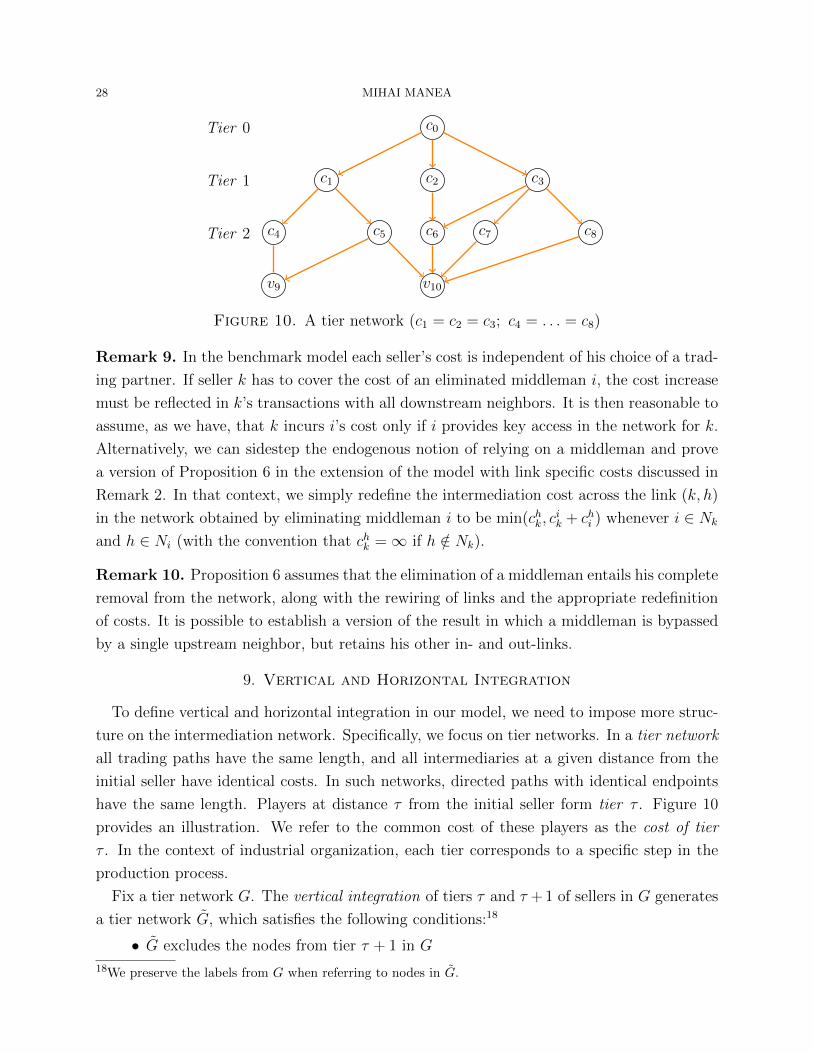
28 MIHAI MANEA
c0Tier 0
Tier 1
Tier 2
c1 c2 c3
c4 c6c5 c7
v9 v10
c8
Figure 10. A tier network (c1 = c2 = c3; c4 = . . . = c8)
Remark 9. In the benchmark model each seller’s cost is independent of his choice of a trad-
ing partner. If seller k has to cover the cost of an eliminated middleman i, the cost increase
must be reflected in k’s transactions with all downstream neighbors. It is then reasonable to
assume, as we have, that k incurs i’s cost only if i provides key access in the network for k.
Alternatively, we can sidestep the endogenous notion of relying on a middleman and prove
a version of Proposition 6 in the extension of the model with link specific costs discussed in
Remark 2. In that context, we simply redefine the intermediation cost across the link (k, h)
in the network obtained by eliminating middleman i to be min(chk, cik + chi ) whenever i ∈ Nk
and h ∈ Ni (with the convention that chk =∞ if h /∈ Nk).
Remark 10. Proposition 6 assumes that the elimination of a middleman entails his complete
removal from the network, along with the rewiring of links and the appropriate redefinition
of costs. It is possible to establish a version of the result in which a middleman is bypassed
by a single upstream neighbor, but retains his other in- and out-links.
9. Vertical and Horizontal Integration
To define vertical and horizontal integration in our model, we need to impose more struc-
ture on the intermediation network. Specifically, we focus on tier networks. In a tier network
all trading paths have the same length, and all intermediaries at a given distance from the
initial seller have identical costs. In such networks, directed paths with identical endpoints
have the same length. Players at distance τ from the initial seller form tier τ . Figure 10
provides an illustration. We refer to the common cost of these players as the cost of tier
τ . In the context of industrial organization, each tier corresponds to a specific step in the
production process.
Fix a tier network G. The vertical integration of tiers τ and τ + 1 of sellers in G generates
a tier network G, which satisfies the following conditions:18
• G excludes the nodes from tier τ + 1 in G
18We preserve the labels from G when referring to nodes in G.
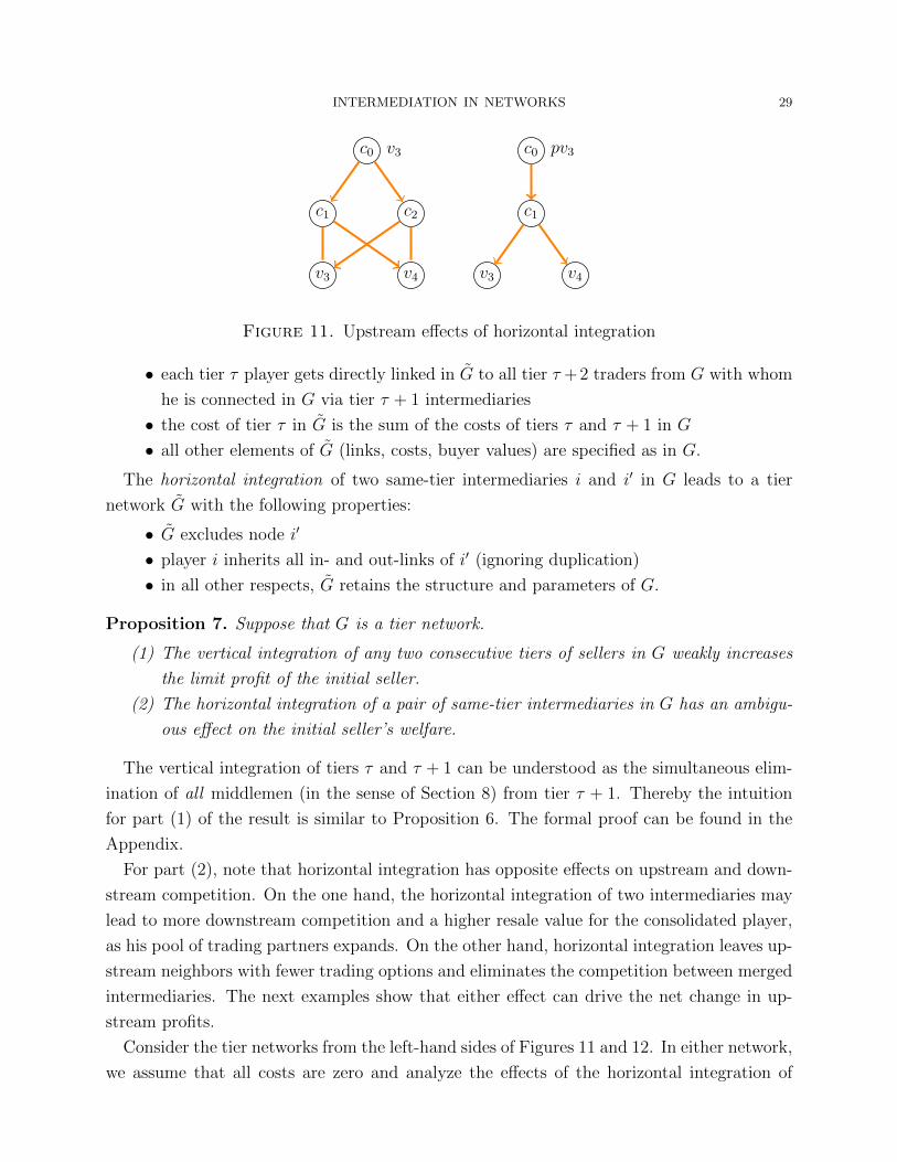
INTERMEDIATION IN NETWORKS 29
c0 v3
c1 c2
v3 v4
c0 pv3
c1
v3 v4
Figure 11. Upstream effects of horizontal integration
• each tier τ player gets directly linked in G to all tier τ +2 traders from G with whom
he is connected in G via tier τ + 1 intermediaries
• the cost of tier τ in G is the sum of the costs of tiers τ and τ + 1 in G
• all other elements of G (links, costs, buyer values) are specified as in G.
The horizontal integration of two same-tier intermediaries i and i′ in G leads to a tier
network G with the following properties:
• G excludes node i′
• player i inherits all in- and out-links of i′ (ignoring duplication)
• in all other respects, G retains the structure and parameters of G.
Proposition 7. Suppose that G is a tier network.
(1) The vertical integration of any two consecutive tiers of sellers in G weakly increases
the limit profit of the initial seller.
(2) The horizontal integration of a pair of same-tier intermediaries in G has an ambigu-
ous effect on the initial seller’s welfare.
The vertical integration of tiers τ and τ + 1 can be understood as the simultaneous elim-
ination of all middlemen (in the sense of Section 8) from tier τ + 1. Thereby the intuition
for part (1) of the result is similar to Proposition 6. The formal proof can be found in the
Appendix.
For part (2), note that horizontal integration has opposite effects on upstream and down-
stream competition. On the one hand, the horizontal integration of two intermediaries may
lead to more downstream competition and a higher resale value for the consolidated player,
as his pool of trading partners expands. On the other hand, horizontal integration leaves up-
stream neighbors with fewer trading options and eliminates the competition between merged
intermediaries. The next examples show that either effect can drive the net change in up-
stream profits.
Consider the tier networks from the left-hand sides of Figures 11 and 12. In either network,
we assume that all costs are zero and analyze the effects of the horizontal integration of
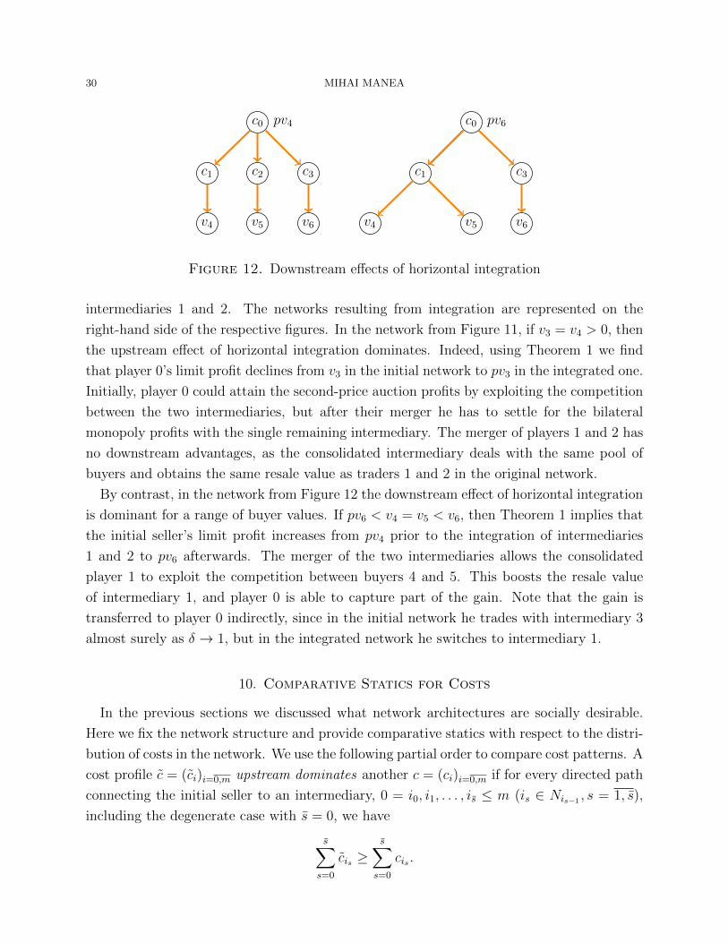
30 MIHAI MANEA
c0 pv4
c1 c2 c3
v4 v5 v6
c0 pv6
c1 c3
v4 v5 v6
Figure 12. Downstream effects of horizontal integration
intermediaries 1 and 2. The networks resulting from integration are represented on the
right-hand side of the respective figures. In the network from Figure 11, if v3 = v4 > 0, then
the upstream effect of horizontal integration dominates. Indeed, using Theorem 1 we find
that player 0’s limit profit declines from v3 in the initial network to pv3 in the integrated one.
Initially, player 0 could attain the second-price auction profits by exploiting the competition
between the two intermediaries, but after their merger he has to settle for the bilateral
monopoly profits with the single remaining intermediary. The merger of players 1 and 2 has
no downstream advantages, as the consolidated intermediary deals with the same pool of
buyers and obtains the same resale value as traders 1 and 2 in the original network.
By contrast, in the network from Figure 12 the downstream effect of horizontal integration
is dominant for a range of buyer values. If pv6 < v4 = v5 < v6, then Theorem 1 implies that
the initial seller’s limit profit increases from pv4 prior to the integration of intermediaries
1 and 2 to pv6 afterwards. The merger of the two intermediaries allows the consolidated
player 1 to exploit the competition between buyers 4 and 5. This boosts the resale value
of intermediary 1, and player 0 is able to capture part of the gain. Note that the gain is
transferred to player 0 indirectly, since in the initial network he trades with intermediary 3
almost surely as δ → 1, but in the integrated network he switches to intermediary 1.
10. Comparative Statics for Costs
In the previous sections we discussed what network architectures are socially desirable.
Here we fix the network structure and provide comparative statics with respect to the distri-
bution of costs in the network. We use the following partial order to compare cost patterns. A
cost profile c = (ci)i=0,m upstream dominates another c = (ci)i=0,m if for every directed path
connecting the initial seller to an intermediary, 0 = i0, i1, . . . , is ≤ m (is ∈ Nis−1 , s = 1, s),
including the degenerate case with s = 0, we have
s∑s=0
cis ≥s∑s=0
cis .
INTERMEDIATION IN NETWORKS 31
Intuitively, c upstream dominates c if costs are relatively more concentrated at the “top”
under c. The next result shows that the downward redistribution of costs in the network
entailed by the shift from c to c weakly benefits the initial seller. The idea is that if the
bilateral monopoly outcome emerges in a transaction between seller i and partner k, then
k “shares” a fraction 1 − p of i’s cost (Remark 4). Hence higher downstream costs reduce
intermediation rents in downstream exchanges, leaving more gains from trade for upstream
players.
Theorem 3. Let c and c be two distinct cost profiles in otherwise identical networks. If c
upstream dominates c, then the initial seller’s limit profit is at least as high under c as under
c.
Remark 11. The notion of cost dominance and Theorem 3 admit straightforward general-
izations to the setting with link specific costs discussed in Remark 2.
Theorem 3 has ramifications for the optimal cost distribution in the applications discussed
in the introduction. In the case of bribery, lobbying, or illegal trade, an intermediary’s
transaction cost represents the risk of getting caught performing the illegal or unethical
activity and the potential penalties. Then crime can be discouraged by ratcheting up the
severity of punishments at the top of the hierarchy. If monitoring expenses need to be
budgeted across the network, the optimal targets for audits and investigations are higher
ranking officials or heads of organized crime.
In the case of manufacturing, costs may capture both production expenditures and taxes.
In order to implement efficient production, Theorem 3 (along with Proposition 4) suggests
that costs have to be pushed downstream to the extent possible. In supply chains, retail
sales taxes are more efficient than value-added taxes. Similarly, subsidies are more effective
at earlier stages of production than at later ones. The result also sheds light on the optimal
allocation of manufacturing processes in supply chains where each step of production is
performed by a tier of specialized firms. If every step involves some essential processes
that require specialization, as well as certain generic tasks (bells and whistles) that can be
performed by downstream firms, then the generic features should be added as far along as
possible in the production of the good.
The result is particularly relevant for situations in which a manufacturer contracts out
specific steps in the production process. In that case trading paths describe competing
suppliers and production technologies (as in the road network interpretation of the model).
When there is flexibility in the order of production steps, the manufacturer prefers dealing
with the costliest suppliers in the last stages. It is also more efficient to grant subsidies to
the main producer rather than to contractors. However, if the manufacturer markets the
32 MIHAI MANEA
finished product directly to final consumers, then retail taxes should be reduced at the cost
of higher taxes for contractors.
Xiao (2012) proves a related result in a setting in which a real estate developer chooses
the order of bargaining with requisite landowners. Despite differences in modeling assump-
tions, our predictions are consistent. The developer should approach owners with smaller
opportunity cost for their land earlier in the bargaining process.
11. Related Literature
Rubinstein and Wolinsky (1987) introduced the first bargaining model of intermediation.
They considered a stationary market with homogeneous populations of buyers, sellers, and
middlemen. In a related model, Duffie et al. (2005) endogenized steady states and search
intensities in the context of an over-the-counter market. In their setting, investors have
stochastically changing types that determine whether they act as buyers or sellers. Investors
may trade with one another, and also with market makers. Due to symmetry assumptions,
the intrinsic intermediation network in either model takes the simple form of a complete
tripartite graph (with links weighted by matching probabilities).
A growing body of recent research explores the effects of general network asymmetries
on intermediation. We first discuss models which share our assumption that a single good
is traded in the network. Goyal and Vega-Redondo (2007) propose a solution whereby the
players essential for trade between the buyer and the seller split the proceeds equally. Their
focus is on strategic network formation under the proposed payoff function.
Siedlarek (2012) considers a model in which traders along a randomly drawn path bargain
over the division of surplus generated by the path. The multilateral nature of his bargaining
protocol eliminates the hold-up problems we identify in our setting. One can show that trade
is asymptotically efficient in Siedlarek’s model. Our models also diverge on a second dimen-
sion. Siedlarek finds support for Goyal’s and Vega-Redondo’s assumption that inessential
intermediaries do not earn any profits.
Gofman (2011) puts forward a solution concept building on the assumption that each
intermediary receives an exogenous share of the gains from trade available in any exchange.
Because of the exogenous division of surplus, his solution concept does not fully capture the
effects of local competition. Farboodi (2014) employs a similar exogenous sharing rule along
intermediation chains in the context of interbank lending.
Choi, Galeotti, and Goyal (2013) consider a static model in which all intermediaries post
prices simultaneously and trade takes place along the least expensive path in the network.
Efficient equilibria always exist in their setting. However, inefficient equilibria may arise due
to coordination failures created by the simultaneity of actions. Condorelli and Galeotti (2012)
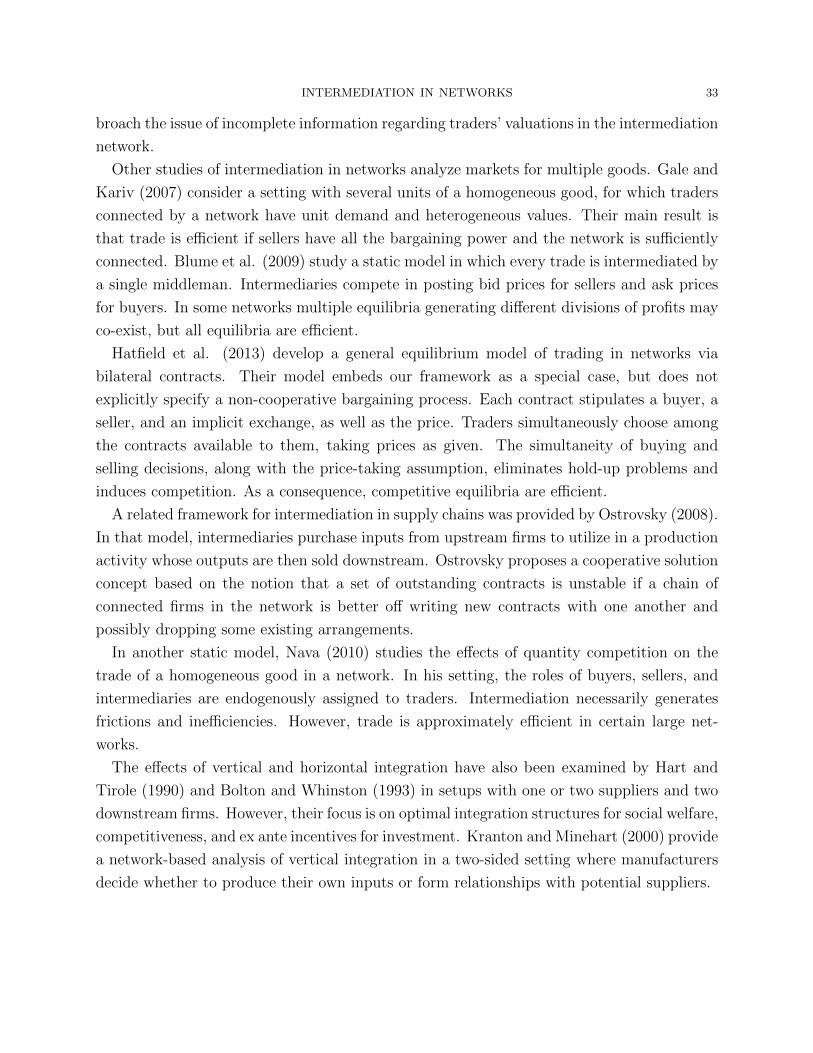
INTERMEDIATION IN NETWORKS 33
broach the issue of incomplete information regarding traders’ valuations in the intermediation
network.
Other studies of intermediation in networks analyze markets for multiple goods. Gale and
Kariv (2007) consider a setting with several units of a homogeneous good, for which traders
connected by a network have unit demand and heterogeneous values. Their main result is
that trade is efficient if sellers have all the bargaining power and the network is sufficiently
connected. Blume et al. (2009) study a static model in which every trade is intermediated by
a single middleman. Intermediaries compete in posting bid prices for sellers and ask prices
for buyers. In some networks multiple equilibria generating different divisions of profits may
co-exist, but all equilibria are efficient.
Hatfield et al. (2013) develop a general equilibrium model of trading in networks via
bilateral contracts. Their model embeds our framework as a special case, but does not
explicitly specify a non-cooperative bargaining process. Each contract stipulates a buyer, a
seller, and an implicit exchange, as well as the price. Traders simultaneously choose among
the contracts available to them, taking prices as given. The simultaneity of buying and
selling decisions, along with the price-taking assumption, eliminates hold-up problems and
induces competition. As a consequence, competitive equilibria are efficient.
A related framework for intermediation in supply chains was provided by Ostrovsky (2008).
In that model, intermediaries purchase inputs from upstream firms to utilize in a production
activity whose outputs are then sold downstream. Ostrovsky proposes a cooperative solution
concept based on the notion that a set of outstanding contracts is unstable if a chain of
connected firms in the network is better off writing new contracts with one another and
possibly dropping some existing arrangements.
In another static model, Nava (2010) studies the effects of quantity competition on the
trade of a homogeneous good in a network. In his setting, the roles of buyers, sellers, and
intermediaries are endogenously assigned to traders. Intermediation necessarily generates
frictions and inefficiencies. However, trade is approximately efficient in certain large net-
works.
The effects of vertical and horizontal integration have also been examined by Hart and
Tirole (1990) and Bolton and Whinston (1993) in setups with one or two suppliers and two
downstream firms. However, their focus is on optimal integration structures for social welfare,
competitiveness, and ex ante incentives for investment. Kranton and Minehart (2000) provide
a network-based analysis of vertical integration in a two-sided setting where manufacturers
decide whether to produce their own inputs or form relationships with potential suppliers.
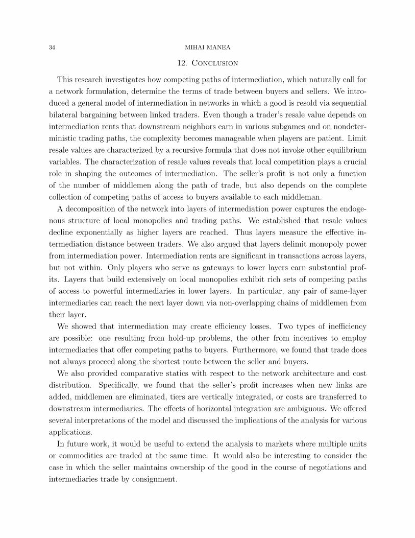
34 MIHAI MANEA
12. Conclusion
This research investigates how competing paths of intermediation, which naturally call for
a network formulation, determine the terms of trade between buyers and sellers. We intro-
duced a general model of intermediation in networks in which a good is resold via sequential
bilateral bargaining between linked traders. Even though a trader’s resale value depends on
intermediation rents that downstream neighbors earn in various subgames and on nondeter-
ministic trading paths, the complexity becomes manageable when players are patient. Limit
resale values are characterized by a recursive formula that does not invoke other equilibrium
variables. The characterization of resale values reveals that local competition plays a crucial
role in shaping the outcomes of intermediation. The seller’s profit is not only a function
of the number of middlemen along the path of trade, but also depends on the complete
collection of competing paths of access to buyers available to each middleman.
A decomposition of the network into layers of intermediation power captures the endoge-
nous structure of local monopolies and trading paths. We established that resale values
decline exponentially as higher layers are reached. Thus layers measure the effective in-
termediation distance between traders. We also argued that layers delimit monopoly power
from intermediation power. Intermediation rents are significant in transactions across layers,
but not within. Only players who serve as gateways to lower layers earn substantial prof-
its. Layers that build extensively on local monopolies exhibit rich sets of competing paths
of access to powerful intermediaries in lower layers. In particular, any pair of same-layer
intermediaries can reach the next layer down via non-overlapping chains of middlemen from
their layer.
We showed that intermediation may create efficiency losses. Two types of inefficiency
are possible: one resulting from hold-up problems, the other from incentives to employ
intermediaries that offer competing paths to buyers. Furthermore, we found that trade does
not always proceed along the shortest route between the seller and buyers.
We also provided comparative statics with respect to the network architecture and cost
distribution. Specifically, we found that the seller’s profit increases when new links are
added, middlemen are eliminated, tiers are vertically integrated, or costs are transferred to
downstream intermediaries. The effects of horizontal integration are ambiguous. We offered
several interpretations of the model and discussed the implications of the analysis for various
applications.
In future work, it would be useful to extend the analysis to markets where multiple units
or commodities are traded at the same time. It would also be interesting to consider the
case in which the seller maintains ownership of the good in the course of negotiations and
intermediaries trade by consignment.

INTERMEDIATION IN NETWORKS 35
Appendix A. Proofs
Proof of Proposition 1. Consider a stationary MPE of the bargaining game with no inter-
mediation and discount factor δ. Let uk denote the expected payoff of player k ∈ N and πj
be the probability that the seller selects buyer j = 1, n for bargaining (following a history
along which the good has not yet been traded) in this equilibrium. Since v1 > c0, the general
arguments from the proof of Theorem 1 establish that the seller reaches an agreement with
conditional probability 1 with any buyer j such that πj > 0. Furthermore, for all j with
πj > 0, we obtain the following payoff equations,
u0 = p(vj − c0 − δuj) + (1− p)δu0
uj = πj (pδuj + (1− p)(vj − c0 − δu0)) .
Expressing variables in terms of u0 (≥ 0), we get
uj =vj − c0
δ− 1− δ + δp
δpu0(A.1)
πj =1− δ + δp
δp− (1− δ)(1− p)(vj − c0)
δp(vj − c0 − u0).(A.2)
The (equilibrium) condition uj ≥ 0 implies that u0 ≤ p(vj−c0)/(1−δ+δp) if πj > 0. It follows
immediately that πj = 0 whenever u0 ≥ p(vj−c0)/(1−δ+δp) (if u0 = p(vj−c0)/(1−δ+δp)
then the right-hand side of (A.2) becomes 0).
Moreover, u0 < p(vj − c0)/(1 − δ + δp) implies that πj > 0. Indeed, if πj = 0 then
uj = 0. The seller has the option to choose buyer j as his bargaining partner in the first
period, which leads to the incentive constraint u0 ≥ p(vj − c0) + (1− p)δu0, or equivalently
u0 ≥ p(vj − c0)/(1− δ + δp).
We established that selection probabilities in any MPE are described by the following
functions of u0
(A.3) πj(u0) =
{1−δ+δpδp− (1−δ)(1−p)(vj−c0)
δp(vj−c0−u0)if u0 < (vj − c0) p
1−δ+δp
0 if u0 ≥ (vj − c0) p1−δ+δp
.
One can easily check that each function πj is strictly decreasing over the interval [0, p(vj −c0)/(1 − δ + δp)] and continuous over [0, p(v1 − c0)/(1 − δ + δp)]. Hence the expression∑n
j=1 πj(u0) is strictly decreasing and varies continuously for u0 ∈ [0, p(v1− c0)/(1− δ+ δp)].
Note thatn∑j=1
πj(0) =|{j|vj > c0}|
δ> 1 and
n∑j=1
πj
(p(v1 − c0)
1− δ + δp
)= 0.
Therefore, there exists a unique u0 for which
(A.4)n∑j=1
πj(u0) = 1.
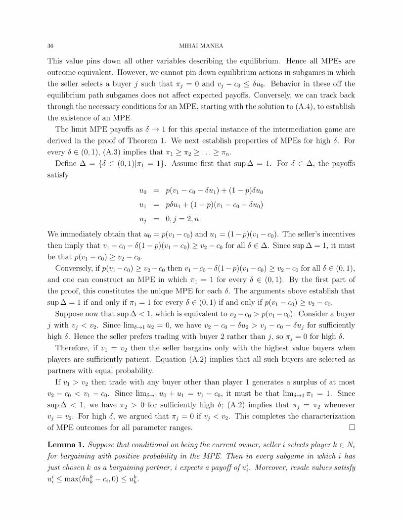
36 MIHAI MANEA
This value pins down all other variables describing the equilibrium. Hence all MPEs are
outcome equivalent. However, we cannot pin down equilibrium actions in subgames in which
the seller selects a buyer j such that πj = 0 and vj − c0 ≤ δu0. Behavior in these off the
equilibrium path subgames does not affect expected payoffs. Conversely, we can track back
through the necessary conditions for an MPE, starting with the solution to (A.4), to establish
the existence of an MPE.
The limit MPE payoffs as δ → 1 for this special instance of the intermediation game are
derived in the proof of Theorem 1. We next establish properties of MPEs for high δ. For
every δ ∈ (0, 1), (A.3) implies that π1 ≥ π2 ≥ . . . ≥ πn.
Define ∆ = {δ ∈ (0, 1)|π1 = 1}. Assume first that sup ∆ = 1. For δ ∈ ∆, the payoffs
satisfy
u0 = p(v1 − c0 − δu1) + (1− p)δu0
u1 = pδu1 + (1− p)(v1 − c0 − δu0)
uj = 0, j = 2, n.
We immediately obtain that u0 = p(v1− c0) and u1 = (1−p)(v1− c0). The seller’s incentives
then imply that v1 − c0 − δ(1− p)(v1 − c0) ≥ v2 − c0 for all δ ∈ ∆. Since sup ∆ = 1, it must
be that p(v1 − c0) ≥ v2 − c0.
Conversely, if p(v1−c0) ≥ v2−c0 then v1−c0−δ(1−p)(v1−c0) ≥ v2−c0 for all δ ∈ (0, 1),
and one can construct an MPE in which π1 = 1 for every δ ∈ (0, 1). By the first part of
the proof, this constitutes the unique MPE for each δ. The arguments above establish that
sup ∆ = 1 if and only if π1 = 1 for every δ ∈ (0, 1) if and only if p(v1 − c0) ≥ v2 − c0.
Suppose now that sup ∆ < 1, which is equivalent to v2− c0 > p(v1− c0). Consider a buyer
j with vj < v2. Since limδ→1 u2 = 0, we have v2 − c0 − δu2 > vj − c0 − δuj for sufficiently
high δ. Hence the seller prefers trading with buyer 2 rather than j, so πj = 0 for high δ.
Therefore, if v1 = v2 then the seller bargains only with the highest value buyers when
players are sufficiently patient. Equation (A.2) implies that all such buyers are selected as
partners with equal probability.
If v1 > v2 then trade with any buyer other than player 1 generates a surplus of at most
v2 − c0 < v1 − c0. Since limδ→1 u0 + u1 = v1 − c0, it must be that limδ→1 π1 = 1. Since
sup ∆ < 1, we have π2 > 0 for sufficiently high δ; (A.2) implies that πj = π2 whenever
vj = v2. For high δ, we argued that πj = 0 if vj < v2. This completes the characterization
of MPE outcomes for all parameter ranges. �
Lemma 1. Suppose that conditional on being the current owner, seller i selects player k ∈ Ni
for bargaining with positive probability in the MPE. Then in every subgame in which i has
just chosen k as a bargaining partner, i expects a payoff of uii. Moreover, resale values satisfy
uii ≤ max(δukk − ci, 0) ≤ ukk.
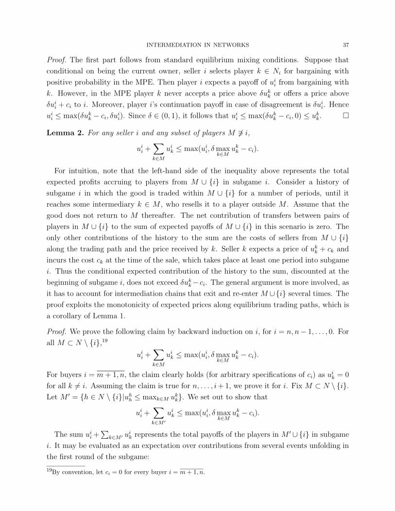
INTERMEDIATION IN NETWORKS 37
Proof. The first part follows from standard equilibrium mixing conditions. Suppose that
conditional on being the current owner, seller i selects player k ∈ Ni for bargaining with
positive probability in the MPE. Then player i expects a payoff of uii from bargaining with
k. However, in the MPE player k never accepts a price above δukk or offers a price above
δuii + ci to i. Moreover, player i’s continuation payoff in case of disagreement is δuii. Hence
uii ≤ max(δukk − ci, δuii). Since δ ∈ (0, 1), it follows that uii ≤ max(δukk − ci, 0) ≤ ukk. �
Lemma 2. For any seller i and any subset of players M 63 i,
uii +∑k∈M
uik ≤ max(uii, δmaxk∈M
ukk − ci).
For intuition, note that the left-hand side of the inequality above represents the total
expected profits accruing to players from M ∪ {i} in subgame i. Consider a history of
subgame i in which the good is traded within M ∪ {i} for a number of periods, until it
reaches some intermediary k ∈ M , who resells it to a player outside M . Assume that the
good does not return to M thereafter. The net contribution of transfers between pairs of
players in M ∪ {i} to the sum of expected payoffs of M ∪ {i} in this scenario is zero. The
only other contributions of the history to the sum are the costs of sellers from M ∪ {i}along the trading path and the price received by k. Seller k expects a price of ukk + ck and
incurs the cost ck at the time of the sale, which takes place at least one period into subgame
i. Thus the conditional expected contribution of the history to the sum, discounted at the
beginning of subgame i, does not exceed δukk− ci. The general argument is more involved, as
it has to account for intermediation chains that exit and re-enter M ∪{i} several times. The
proof exploits the monotonicity of expected prices along equilibrium trading paths, which is
a corollary of Lemma 1.
Proof. We prove the following claim by backward induction on i, for i = n, n− 1, . . . , 0. For
all M ⊂ N \ {i},19
uii +∑k∈M
uik ≤ max(uii, δmaxk∈M
ukk − ci).
For buyers i = m+ 1, n, the claim clearly holds (for arbitrary specifications of ci) as uik = 0
for all k 6= i. Assuming the claim is true for n, . . . , i+ 1, we prove it for i. Fix M ⊂ N \ {i}.Let M ′ = {h ∈ N \ {i}|uhh ≤ maxk∈M ukk}. We set out to show that
uii +∑k∈M ′
uik ≤ max(uii, δmaxk∈M
ukk − ci).
The sum uii +∑
k∈M ′ uik represents the total payoffs of the players in M ′ ∪ {i} in subgame
i. It may be evaluated as an expectation over contributions from several events unfolding in
the first round of the subgame:
19By convention, let ci = 0 for every buyer i = m+ 1, n.
38 MIHAI MANEA
(1) player i trades with some player h ∈M ′;
(2) player i trades with some player h /∈M ′;
(3) player i does not reach an agreement with his selected bargaining partner.
In the first event, players i and h exchange the good for a payment. Besides the change
in ownership, the net contribution of this transaction to the total payoffs of i and h is the
cost ci. The conditional continuation payoff of each player k ∈M ′ is given by δuhk. The sum
of continuation payoffs of the players in M ′ ∪ {i} conditional on the transaction between i
and h is thus
δ∑k∈M ′
uhk − ci.
By the induction hypothesis applied for player h (h ∈ Ni ⇒ h > i) and the set M ′ \ {h}, the
expression above does not exceed δmax(uhh, δmaxk∈M ′\{h} ukk−ch)−ci ≤ δmaxk∈M ′ u
kk−ci =
δmaxk∈M ukk − ci.In the second event, player i trades with some h /∈ M ′. By definition, uhh > maxk∈M ′ u
kk.
Since Lemma 1 implies that resale values are non-decreasing along every path on which trade
takes place with positive probability, it must be that once h acquires the good, no player in
M ′ ever purchases the good at a later stage. Thus conditional on i selling the good to h,
the expected payoffs of all players in M ′ are 0. By Lemma 1, player i’s conditional expected
payoff (when event (2) has positive probability) is uii. Hence event (2) contributes to the
sum of payoffs of the players in M ′ ∪ {i} with the amount uii.
The third event contributes to the expectation with a term δ(uii +∑
k∈M ′ uik).
Since uii +∑
k∈M ′ uik is evaluated as an expectation of contributions from events of one of
the three types analyzed above, it must be that
uii +∑k∈M ′
uik ≤ max
(uii, δmax
k∈Mukk − ci, δ(uii +
∑k∈M ′
uik)
).
Then uii +∑
k∈M ′ uik ≥ 0, uii ≥ 0 and δ ∈ (0, 1) imply that
uii +∑k∈M ′
uik ≤ max(uii, δmaxk∈M
ukk − ci).
As M ⊂M ′ and uik ≥ 0 for all k ∈M ′, the latter inequality leads to
uii +∑k∈M
uik ≤ max(uii, δmaxk∈M
ukk − ci),
which concludes the proof of the inductive step. �
Proof of Theorem 1. We prove by backward induction on i, for i = n, n − 1, . . . , 0, that
uii converges as δ goes to 1 to a limit ri, which satisfies ri = vi for i = m+ 1, n and
ri = max(p(rINi− ci), rIINi
− ci, 0) for i = 0,m. The base cases i = n, . . . ,m+1 (corresponding
INTERMEDIATION IN NETWORKS 39
to buyers) are trivially verified. Assuming that the induction hypothesis holds for players
n, . . . , i+ 1, we seek to prove it for seller i (≤ m).
Let ∆ = {δ ∈ (0, 1)|δmaxk∈Niukk ≤ ci}. If sup ∆ = 1, then the induction hypothesis
implies that maxk∈Niδukk converges to rINi
≤ ci as δ → 1. Hence the maximum gains that i
can create by trading with any of his neighbors vanish as δ → 1. It follows that uii converges
to 0 as δ → 1, so limδ→1 uii = 0 = max(p(rINi
− ci), rIINi− ci, 0).
For the rest of the proof, assume that sup ∆ < 1 and restrict attention to δ > sup ∆. Then
rINi≥ ci and δmaxk∈Ni
ukk > ci. Fix k1 ∈ arg maxk∈Niukk. By Lemma 1,
(A.5) uii ≤ max(δuk1
k1 − ci, 0) = δuk1
k1 − ci.
Then Lemma 2 implies that
(A.6) uii +∑k∈Ni
uik ≤ δuk1
k1 − ci.
If δuk1
k1 − ci ≤ δuik1 then the inequality above leads to
uii +∑k∈Ni
uik ≤ δuk1
k1 − ci ≤ δuik1 ,
which is possible only if uik = 0 for all k ∈ Ni ∪ {i}. However, if uik1 = 0 then player i
can select k1 for bargaining and offer him an acceptable price arbitrarily close to δuk1
k1 . This
deviation leads to a profit approaching δuk1
k1 − ci > 0 in the event that i is chosen as the
proposer, contradicting uii = 0.
Hence δuk1
k1 − ci > δuik1 . Since player k1 accepts any price z with δuk1
k1 − z > δuik1 , player
i can secure a positive profit by bargaining with k1 and, when selected to make an offer to
k1, proposing a price arbitrarily close to δuk1
k1 − δuik1 > ci. Thus uii > 0.
Assume that the current seller i selects k ∈ Ni for bargaining with positive probability.
By Lemma 1, player i expects a payoff of uii conditional on choosing k. Note that player
k would never offer i a price higher than δuii + ci, and i’s continuation payoff in case of
disagreement is δuii. Since uii > 0, it must be that k is willing to accept a price offer z from
i with z − ci > uii. Then δukk − z ≥ δuik, which leads to δukk − δuik ≥ z > uii + ci. It follows
that δ(uii + uik) < δukk − ci. Standard arguments then imply that conditional on i selecting
k as a bargaining partner, the two players trade with probability 1. When selected as the
proposer, either player offers a price that makes the opponent indifferent between accepting
and rejecting the offer. The equilibrium prices offered by i and k are δukk − δuik and δuii + ci,
respectively.
40 MIHAI MANEA
Let πk denote the probability that seller i selects player k ∈ Ni for bargaining in subgame
i. The arguments above lead to the following equilibrium conditions for all k ∈ Ni,
uii ≥ p(δukk − ci − δuik) + (1− p)δuii, with equality if πk > 0(A.7)
uik = πk(pδuik + (1− p)(δukk − ci − δuii)
)+
∑h∈Ni\{k}
πhδuhk.(A.8)
For all h ∈ Ni with πh > 0, seller i’s incentive constraints (A.7) lead to δuhh − ci − δuih ≥δuk
1
k1 − ci − δuik1 , or equivalently,
(A.9) uk1
k1 − uhh ≤ uik1 − uih.
By Lemma 2, we have uhh+uhk1 ≤ max(uhh, δuk1
k1− ch), which along with δ ∈ (0, 1) and ch ≥ 0,
implies that uhk1 ≤ max(0, uk1
k1 − uhh) = uk1
k1 − uhh. Then (A.9) leads to
(A.10) uhk1 ≤ uik1 − uih ≤ uik1 .
Combining (A.10) with (A.8) for k = k1, we obtain
uik1 ≤ πk1
(pδuik1 + (1− p)(δuk1
k1 − ci − δuii))
+∑
h∈Ni\{k1}
πhδuik1 .
Since uik1 ≥ 0 and δuk1
k1 − ci − δuii ≥ 0 (A.5), it follows that
uik1 ≤πk1
1− δ∑
h∈Ni\{k1} πh
(pδuik1 + (1− p)(δuk1
k1 − ci − δuii))≤ pδuik1+(1−p)(δuk1
k1−ci−δuii),
which leads to
(A.11) uik1 ≤(1− p)(δuk1
k1 − ci − δuii)1− pδ
.
By the incentive constraint (A.7) for k = k1,
(A.12) uii ≥p(δuk
1
k1 − ci − δuik1)
1− (1− p)δ.
Substituting the bound on uik1 from (A.11) into (A.12) and collecting the uii terms, we find
that uii ≥ p(δuk1
k1−ci). By the induction hypothesis, uk1
k1 converges to rINias δ → 1. Therefore,
lim infδ→1 uii ≥ p(rINi
− ci).For k = k1, (A.7) can be rewritten as uii(1− (1−p)δ)+pδuik1 ≥ p(δuk
1
k1− ci), which implies
that (recall that k1 is a function of δ)
lim infδ→1
(uii + uik1
)≥ lim
δ→1uk
1
k1 − ci = rINi− ci.
Since (A.6) holds for every δ ∈ ∆, we obtain
lim supδ→1
(uii +
∑k∈Ni
uik
)≤ rINi
− ci.
INTERMEDIATION IN NETWORKS 41
Consider a player k2 ∈ arg maxk∈Ni\{k1} ukk (k2 is also a function of δ). The last two display
equations imply that limδ→1 uik2 = 0. The incentive constraint (A.7) for k = k2 leads to
uii(1−(1−p)δ)+pδuik2 ≥ p(δuk2
k2−ci). Since limδ→1 uik2 = 0 and, by the induction hypothesis,
limδ→1 uk2
k2 = rIINi, we obtain lim infδ→1 u
ii ≥ rIINi
− ci.Thus far, we established that
(A.13) lim infδ→1
uii ≥ max(p(rINi− ci), rIINi
− ci).
We next prove by contradiction that
(A.14) lim supδ→1
uii ≤ max(p(rINi− ci), rIINi
− ci).
Suppose that (A.14) does not hold. Then there exists a sequence S of δ approaching 1,20
along which uii converges to a limit greater than max(p(rINi− ci), rIINi
− ci). S can be chosen
to satisfy in addition one of the following properties:
(i) there exists k ∈ Ni such that for all δ ∈ S, current seller i selects k for bargaining with
conditional probability 1 in the MPE;
(ii) there exist k 6= h ∈ Ni such that for all δ ∈ S, ukk ≥ uhh and current seller i bargains
with positive conditional probability with both k and h.
In case (i), the analysis above establishes that for all δ ∈ S,
uii = p(δukk − ci − δuik) + (1− p)δuiiuik = pδuik + (1− p)(δukk − ci − δuii).
The system of equations is immediately solved to obtain uii = p(δukk−ci). Then the induction
hypothesis implies that limδ∈S uii = p(rk − ci) ≤ p(rINi
− ci).In case (ii), it must be that uii = p(δuhh − ci − δuih) + (1− p)δuii, which implies that
(A.15) uii(1− (1− p)δ) ≤ p(δuhh − ci).
Note that ukk ≥ uhh, along with the induction hypothesis, leads to rk = limδ→1 ukk ≥
limδ→1 uhh = rh. In particular, rh ≤ rIINi
. Taking the limit for δ along S in (A.15), we
immediately find that limδ∈S uii ≤ rIINi
− ci.In either case, we obtained a contradiction with the assumption that limδ∈S u
ii > max(p(rINi
−ci), r
IINi− ci). Therefore, (A.14) holds, implying along with (A.13) that uii converges as δ → 1
to ri = max(p(rINi− ci), r
IINi− ci) = max(p(rINi
− ci), rIINi− ci, 0) (recall that rINi
≥ ci if
sup ∆ < 1). This completes the proof of the inductive step. �
Proof of Proposition 2. We construct recursively a profile (ukk′)k,k′∈N that describes the pay-
offs in each subgame in an MPE of the intermediation game. For k = m+ 1, n we simply
20To simplify notation, we write δ ∈ S to represent the fact that δ appears in the sequence S and use theshorthand limδ→S1 f for the limit of a function f : (0, 1)→ R along the sequence S.
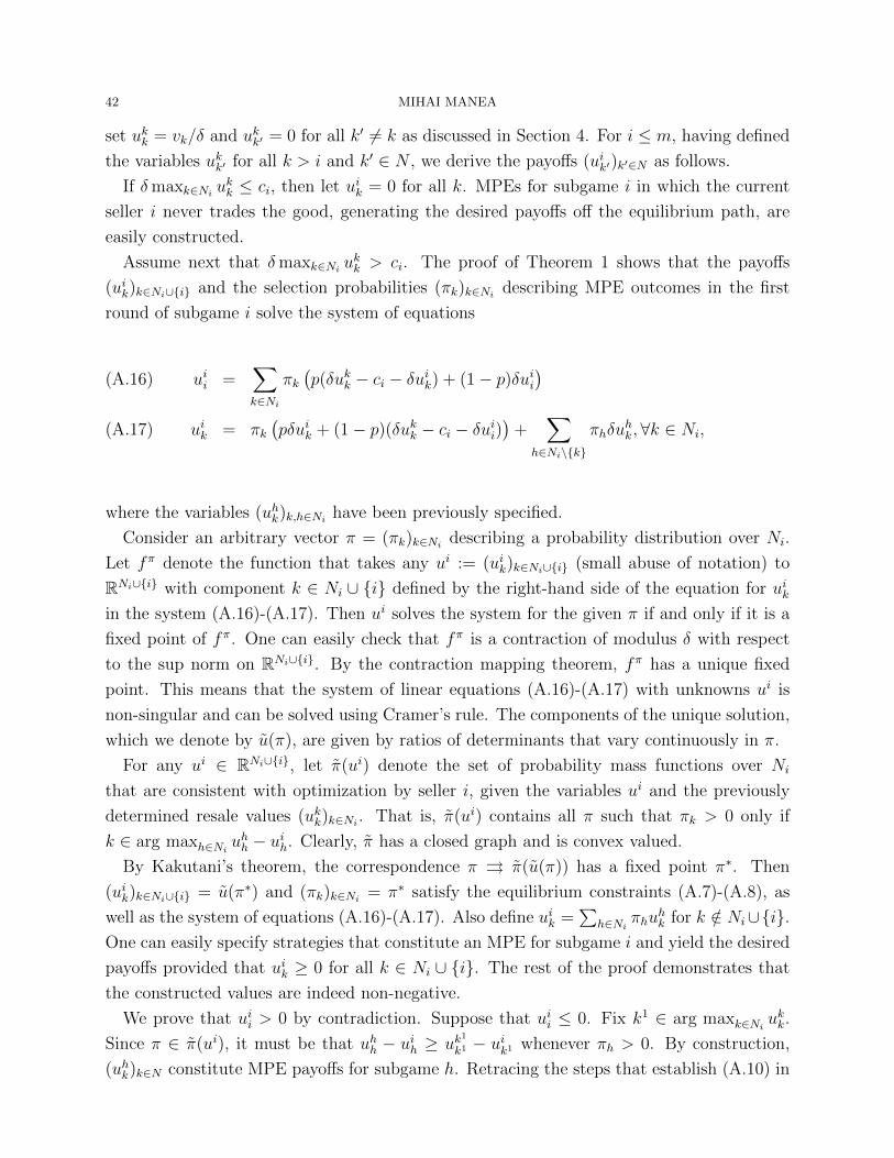
42 MIHAI MANEA
set ukk = vk/δ and ukk′ = 0 for all k′ 6= k as discussed in Section 4. For i ≤ m, having defined
the variables ukk′ for all k > i and k′ ∈ N , we derive the payoffs (uik′)k′∈N as follows.
If δmaxk∈Niukk ≤ ci, then let uik = 0 for all k. MPEs for subgame i in which the current
seller i never trades the good, generating the desired payoffs off the equilibrium path, are
easily constructed.
Assume next that δmaxk∈Niukk > ci. The proof of Theorem 1 shows that the payoffs
(uik)k∈Ni∪{i} and the selection probabilities (πk)k∈Nidescribing MPE outcomes in the first
round of subgame i solve the system of equations
uii =∑k∈Ni
πk(p(δukk − ci − δuik) + (1− p)δuii
)(A.16)
uik = πk(pδuik + (1− p)(δukk − ci − δuii)
)+
∑h∈Ni\{k}
πhδuhk,∀k ∈ Ni,(A.17)
where the variables (uhk)k,h∈Nihave been previously specified.
Consider an arbitrary vector π = (πk)k∈Nidescribing a probability distribution over Ni.
Let fπ denote the function that takes any ui := (uik)k∈Ni∪{i} (small abuse of notation) to
RNi∪{i} with component k ∈ Ni ∪ {i} defined by the right-hand side of the equation for uikin the system (A.16)-(A.17). Then ui solves the system for the given π if and only if it is a
fixed point of fπ. One can easily check that fπ is a contraction of modulus δ with respect
to the sup norm on RNi∪{i}. By the contraction mapping theorem, fπ has a unique fixed
point. This means that the system of linear equations (A.16)-(A.17) with unknowns ui is
non-singular and can be solved using Cramer’s rule. The components of the unique solution,
which we denote by u(π), are given by ratios of determinants that vary continuously in π.
For any ui ∈ RNi∪{i}, let π(ui) denote the set of probability mass functions over Ni
that are consistent with optimization by seller i, given the variables ui and the previously
determined resale values (ukk)k∈Ni. That is, π(ui) contains all π such that πk > 0 only if
k ∈ arg maxh∈Niuhh − uih. Clearly, π has a closed graph and is convex valued.
By Kakutani’s theorem, the correspondence π ⇒ π(u(π)) has a fixed point π∗. Then
(uik)k∈Ni∪{i} = u(π∗) and (πk)k∈Ni= π∗ satisfy the equilibrium constraints (A.7)-(A.8), as
well as the system of equations (A.16)-(A.17). Also define uik =∑
h∈Niπhu
hk for k /∈ Ni∪{i}.
One can easily specify strategies that constitute an MPE for subgame i and yield the desired
payoffs provided that uik ≥ 0 for all k ∈ Ni ∪ {i}. The rest of the proof demonstrates that
the constructed values are indeed non-negative.
We prove that uii > 0 by contradiction. Suppose that uii ≤ 0. Fix k1 ∈ arg maxk∈Niukk.
Since π ∈ π(ui), it must be that uhh − uih ≥ uk1
k1 − uik1 whenever πh > 0. By construction,
(uhk)k∈N constitute MPE payoffs for subgame h. Retracing the steps that establish (A.10) in
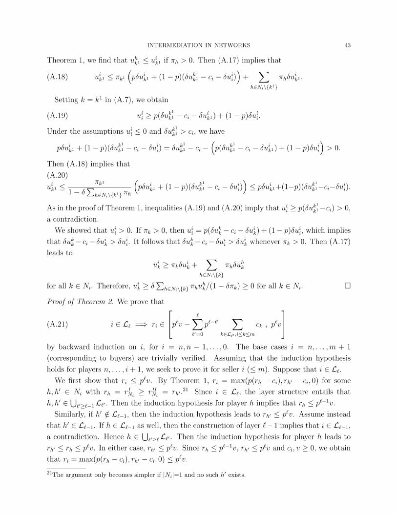
INTERMEDIATION IN NETWORKS 43
Theorem 1, we find that uhk1 ≤ uik1 if πh > 0. Then (A.17) implies that
(A.18) uik1 ≤ πk1
(pδuik1 + (1− p)(δuk1
k1 − ci − δuii))
+∑
h∈Ni\{k1}
πhδuik1 .
Setting k = k1 in (A.7), we obtain
(A.19) uii ≥ p(δuk1
k1 − ci − δuik1) + (1− p)δuii.
Under the assumptions uii ≤ 0 and δuk1
k1 > ci, we have
pδuik1 + (1− p)(δuk1
k1 − ci − δuii) = δuk1
k1 − ci −(p(δuk
1
k1 − ci − δuik1) + (1− p)δuii)> 0.
Then (A.18) implies that
(A.20)
uik1 ≤πk1
1− δ∑
h∈Ni\{k1} πh
(pδuik1 + (1− p)(δuk1
k1 − ci − δuii))≤ pδuik1+(1−p)(δuk1
k1−ci−δuii).
As in the proof of Theorem 1, inequalities (A.19) and (A.20) imply that uii ≥ p(δuk1
k1−ci) > 0,
a contradiction.
We showed that uii > 0. If πk > 0, then uii = p(δukk − ci − δuik) + (1− p)δuii, which implies
that δukk− ci− δuik > δuii. It follows that δukk− ci− δuii > δuik whenever πk > 0. Then (A.17)
leads to
uik ≥ πkδuik +
∑h∈Ni\{k}
πhδuhk
for all k ∈ Ni. Therefore, uik ≥ δ∑
h∈Ni\{k} πhuhk/(1− δπk) ≥ 0 for all k ∈ Ni. �
Proof of Theorem 2. We prove that
(A.21) i ∈ L` =⇒ ri ∈
p`v − ∑`′=0
p`−`′ ∑k∈L`′ ,i≤k≤m
ck , p`v
by backward induction on i, for i = n, n − 1, . . . , 0. The base cases i = n, . . . ,m + 1
(corresponding to buyers) are trivially verified. Assuming that the induction hypothesis
holds for players n, . . . , i+ 1, we seek to prove it for seller i (≤ m). Suppose that i ∈ L`.We first show that ri ≤ p`v. By Theorem 1, ri = max(p(rh − ci), rh′ − ci, 0) for some
h, h′ ∈ Ni with rh = rINi≥ rIINi
= rh′ .21 Since i ∈ L`, the layer structure entails that
h, h′ ∈⋃`′≥`−1 L`′ . Then the induction hypothesis for player h implies that rh ≤ p`−1v.
Similarly, if h′ /∈ L`−1, then the induction hypothesis leads to rh′ ≤ p`v. Assume instead
that h′ ∈ L`−1. If h ∈ L`−1 as well, then the construction of layer `−1 implies that i ∈ L`−1,
a contradiction. Hence h ∈⋃`′≥` L`′ . Then the induction hypothesis for player h leads to
rh′ ≤ rh ≤ p`v. In either case, rh′ ≤ p`v. Since rh ≤ p`−1v, rh′ ≤ p`v and ci, v ≥ 0, we obtain
that ri = max(p(rh − ci), rh′ − ci, 0) ≤ p`v.
21The argument only becomes simpler if |Ni|=1 and no such h′ exists.
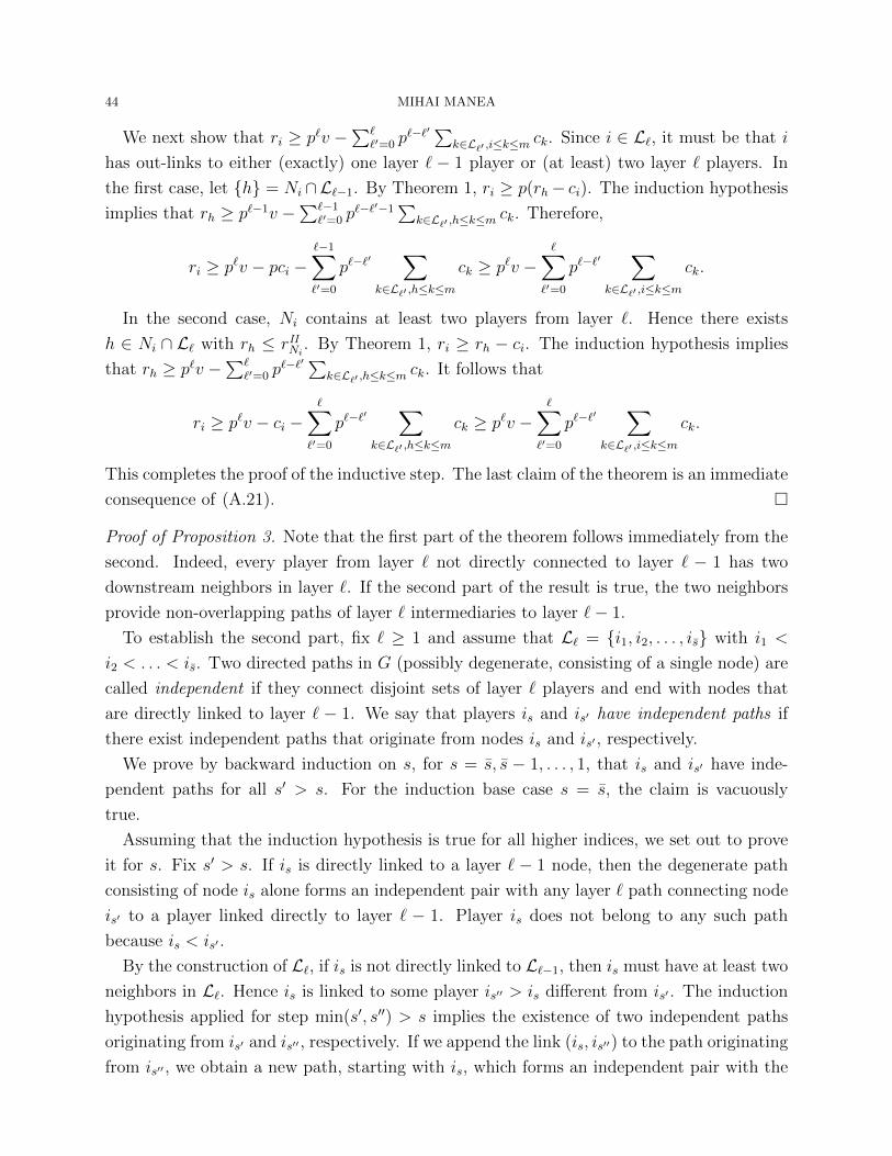
44 MIHAI MANEA
We next show that ri ≥ p`v −∑`
`′=0 p`−`′∑
k∈L`′ ,i≤k≤mck. Since i ∈ L`, it must be that i
has out-links to either (exactly) one layer ` − 1 player or (at least) two layer ` players. In
the first case, let {h} = Ni ∩L`−1. By Theorem 1, ri ≥ p(rh− ci). The induction hypothesis
implies that rh ≥ p`−1v −∑`−1
`′=0 p`−`′−1
∑k∈L`′ ,h≤k≤m
ck. Therefore,
ri ≥ p`v − pci −`−1∑`′=0
p`−`′ ∑k∈L`′ ,h≤k≤m
ck ≥ p`v −∑`′=0
p`−`′ ∑k∈L`′ ,i≤k≤m
ck.
In the second case, Ni contains at least two players from layer `. Hence there exists
h ∈ Ni ∩ L` with rh ≤ rIINi. By Theorem 1, ri ≥ rh − ci. The induction hypothesis implies
that rh ≥ p`v −∑`
`′=0 p`−`′∑
k∈L`′ ,h≤k≤mck. It follows that
ri ≥ p`v − ci −∑`′=0
p`−`′ ∑k∈L`′ ,h≤k≤m
ck ≥ p`v −∑`′=0
p`−`′ ∑k∈L`′ ,i≤k≤m
ck.
This completes the proof of the inductive step. The last claim of the theorem is an immediate
consequence of (A.21). �
Proof of Proposition 3. Note that the first part of the theorem follows immediately from the
second. Indeed, every player from layer ` not directly connected to layer ` − 1 has two
downstream neighbors in layer `. If the second part of the result is true, the two neighbors
provide non-overlapping paths of layer ` intermediaries to layer `− 1.
To establish the second part, fix ` ≥ 1 and assume that L` = {i1, i2, . . . , is} with i1 <
i2 < . . . < is. Two directed paths in G (possibly degenerate, consisting of a single node) are
called independent if they connect disjoint sets of layer ` players and end with nodes that
are directly linked to layer ` − 1. We say that players is and is′ have independent paths if
there exist independent paths that originate from nodes is and is′ , respectively.
We prove by backward induction on s, for s = s, s − 1, . . . , 1, that is and is′ have inde-
pendent paths for all s′ > s. For the induction base case s = s, the claim is vacuously
true.
Assuming that the induction hypothesis is true for all higher indices, we set out to prove
it for s. Fix s′ > s. If is is directly linked to a layer ` − 1 node, then the degenerate path
consisting of node is alone forms an independent pair with any layer ` path connecting node
is′ to a player linked directly to layer ` − 1. Player is does not belong to any such path
because is < is′ .
By the construction of L`, if is is not directly linked to L`−1, then is must have at least two
neighbors in L`. Hence is is linked to some player is′′ > is different from is′ . The induction
hypothesis applied for step min(s′, s′′) > s implies the existence of two independent paths
originating from is′ and is′′ , respectively. If we append the link (is, is′′) to the path originating
from is′′ , we obtain a new path, starting with is, which forms an independent pair with the
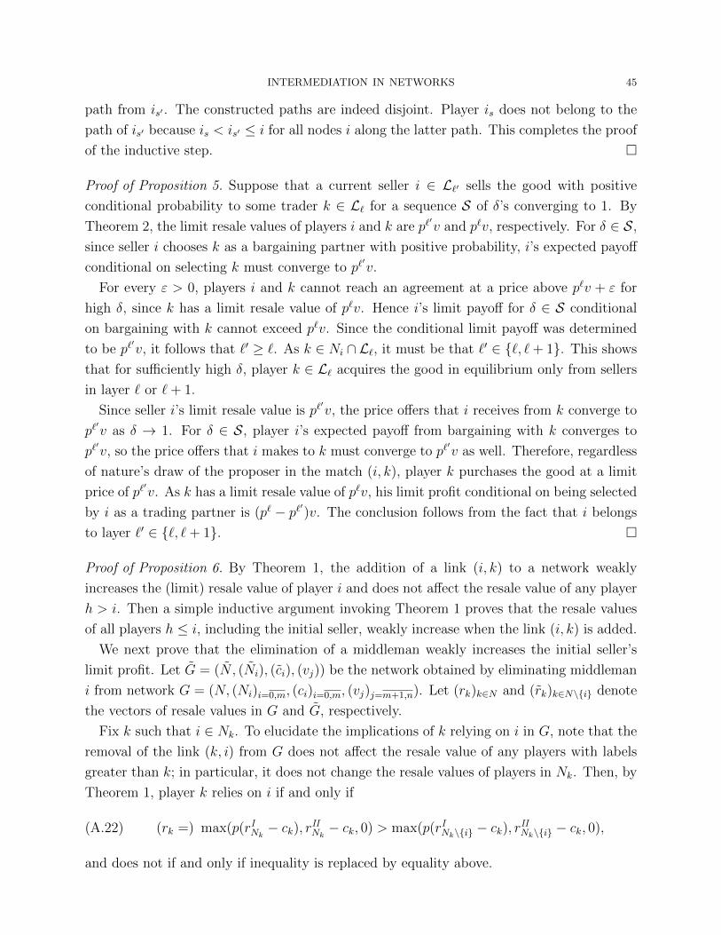
INTERMEDIATION IN NETWORKS 45
path from is′ . The constructed paths are indeed disjoint. Player is does not belong to the
path of is′ because is < is′ ≤ i for all nodes i along the latter path. This completes the proof
of the inductive step. �
Proof of Proposition 5. Suppose that a current seller i ∈ L`′ sells the good with positive
conditional probability to some trader k ∈ L` for a sequence S of δ’s converging to 1. By
Theorem 2, the limit resale values of players i and k are p`′v and p`v, respectively. For δ ∈ S,
since seller i chooses k as a bargaining partner with positive probability, i’s expected payoff
conditional on selecting k must converge to p`′v.
For every ε > 0, players i and k cannot reach an agreement at a price above p`v + ε for
high δ, since k has a limit resale value of p`v. Hence i’s limit payoff for δ ∈ S conditional
on bargaining with k cannot exceed p`v. Since the conditional limit payoff was determined
to be p`′v, it follows that `′ ≥ `. As k ∈ Ni ∩ L`, it must be that `′ ∈ {`, `+ 1}. This shows
that for sufficiently high δ, player k ∈ L` acquires the good in equilibrium only from sellers
in layer ` or `+ 1.
Since seller i’s limit resale value is p`′v, the price offers that i receives from k converge to
p`′v as δ → 1. For δ ∈ S, player i’s expected payoff from bargaining with k converges to
p`′v, so the price offers that i makes to k must converge to p`
′v as well. Therefore, regardless
of nature’s draw of the proposer in the match (i, k), player k purchases the good at a limit
price of p`′v. As k has a limit resale value of p`v, his limit profit conditional on being selected
by i as a trading partner is (p` − p`′)v. The conclusion follows from the fact that i belongs
to layer `′ ∈ {`, `+ 1}. �
Proof of Proposition 6. By Theorem 1, the addition of a link (i, k) to a network weakly
increases the (limit) resale value of player i and does not affect the resale value of any player
h > i. Then a simple inductive argument invoking Theorem 1 proves that the resale values
of all players h ≤ i, including the initial seller, weakly increase when the link (i, k) is added.
We next prove that the elimination of a middleman weakly increases the initial seller’s
limit profit. Let G = (N , (Ni), (ci), (vj)) be the network obtained by eliminating middleman
i from network G = (N, (Ni)i=0,m, (ci)i=0,m, (vj)j=m+1,n). Let (rk)k∈N and (rk)k∈N\{i} denote
the vectors of resale values in G and G, respectively.
Fix k such that i ∈ Nk. To elucidate the implications of k relying on i in G, note that the
removal of the link (k, i) from G does not affect the resale value of any players with labels
greater than k; in particular, it does not change the resale values of players in Nk. Then, by
Theorem 1, player k relies on i if and only if
(A.22) (rk =) max(p(rINk− ck), rIINk
− ck, 0) > max(p(rINk\{i} − ck), rIINk\{i} − ck, 0),
and does not if and only if inequality is replaced by equality above.
46 MIHAI MANEA
We now show that if k relies on i then rk ≤ ri − ck. Indeed, if k relies on i then (A.22)
implies that either rk = p(rINk− ck) > p(rINk\{i} − ck) or rk = rIINk
− ck > rIINk\{i} − ck. In the
first case, we have rINk> rINk\{i}, which means that ri = rINk
. Hence rk = p(ri − ck) ≥ 0,
giving rise to rk ≤ ri− ck. In the second case, we obtain that rIINk> rIINk\{i}, which is possible
only if ri ≥ rIINk. Then rk = rIINk
−ck ≤ ri−ck. In both cases, we established that rk ≤ ri−ck.We prove by reverse induction on k, for k = n, n− 1, . . . , i + 1, i− 1, . . . , 0, that rk ≤ rk.
For the base cases k = n, n − 1, . . . , i + 1, it is obvious that rk = rk. Assuming that the
induction hypothesis holds for all players different from i with labels greater than k, we aim
to prove it for player k < i. Consider two cases:
(i) i ∈ Nk and k relies on i;
(ii) i /∈ Nk or i ∈ Nk but k does not rely on i.
In case (i), since k relies on i, we have rk ≤ ri − ck. Then Theorem 1 leads to
rk ≤ ri − ck = max(p(rINi− ci)− ck, rIINi
− ci − ck,−ck)
≤ max(p(rINi− ck − ci), rIINi
− ck − ci, 0) = max(p(rINi− ck), rIINi
− ck, 0)
≤ max(p(rINk− ck), rIINk
− ck, 0) = rk.
The sequence of equalities and inequalities above uses the following conditions: ck ≥ 0, rh =
rh, ∀h ∈ Ni ⊂ Nk and ck = ck + ci.
In case (ii), either i /∈ Nk or i ∈ Nk and k does not rely on i implies that rk =
max(p(rINk\{i}− ck), rIINk\{i}− ck, 0). By the induction hypothesis, rh ≤ rh for all h ∈ Nk \{i}.
Theorem 1 then leads to
rk = max(p(rINk\{i} − ck), rIINk\{i} − ck, 0) ≤ max(p(rINk\{i} − ck), r
IINk\{i} − ck, 0) = rk.
This completes the proof of the induction step. Step k = 0 yields the desired inequality,
r0 ≤ r0. �
Proof of Proposition 7.1. Consider the network G obtained from the vertical integration of
tiers τ and τ + 1 in a tier network G. Let (Ni, ci, ri) and (Ni, ci, ri) denote the sets of
downstream neighbors, the transaction costs, and the limit resale values of seller i in G and
G (when defined), respectively.
Let i be a seller from tier τ in G. Suppose that k ∈ arg maxh∈Nirh. Player k is an
intermediary belonging to tier τ + 1 in G. Note that the pattern of connections among
traders situated downstream of tiers τ + 2 in G and τ + 1 in G is identical in G and G,
respectively. Then rh = rh for all h ∈ Ni, as Ni is a subset of tier τ + 2 in G as well as tier
τ + 1 in G.
INTERMEDIATION IN NETWORKS 47
By Theorem 1, ri = max(p(rINi− ci), rIINi
− ci, 0) ≤ max(rk − ci, 0). Therefore,
ri ≤ max(rk − ci, 0)
= max(p(rINk− ck)− ci, rIINk
− ci − ck, 0)
≤ max(p(rINk− ci − ck), rIINk
− ci − ck, 0)
≤ max(p(rINi− ci), rIINi
− ci, 0)
= ri,
where the last inequality uses the following consequences of vertical integration: ci = ci +
ck, Nk ⊂⋃h∈Ni
Nh = Ni, and rh = rh for all h ∈ Ni.
We established that ri ≥ ri for every seller i from tier τ in G. Since the connections
among tiers 0 through τ and the costs of tiers 0 through τ − 1 are identical in G and G, a
simple inductive argument invoking Theorem 1 shows that ri ≥ ri for every trader i in tiers
0, . . . , τ − 1. In particular, r0 ≥ r0. �
Proof of Theorem 3. It is useful to generalize the concept of cost domination as follows. For
κ ≥ 0, a cost pattern c κ-dominates another c at some node i ∈ N if for every path of sellers
originating at i, i = i0, i1, . . . , is ≤ m (is ∈ Nis−1 , s = 1, s), including the case s = 0,
(A.23) κ+s∑s=0
cis ≥s∑s=0
cis .
The condition above is vacuously satisfied if i is a buyer since there are no seller paths
originating at i in that case.
We prove by backward induction on i, for i = n, n − 1, . . . , 0, that for any c and c such
that c κ-dominates c at node i for κ ≥ 0, we have ri + κ ≥ ri, where ri and ri denote player
i’s limit resale values in the intermediation game under cost structures c and c, respectively.
The result to prove is a special case of the claim above, for i = 0 and κ = 0.
For buyers i, we have ri = ri = vi, which along with κ ≥ 0 proves the base cases
i = n, . . . ,m+ 1. Assuming that the induction hypothesis holds for players n, . . . , i+ 1, we
seek to prove it for seller i (≤ m). Suppose that c κ-dominates c at i, and let r and r denote
the vectors of resale values under c and c, respectively.
Fix k ∈ Ni. Considering all seller paths starting with the link (i, k) in (A.23), we can check
that c (κ+ ci − ci)-dominates c at k. The domination inequality (A.23) for the degenerate
path consisting of the single node i becomes κ + ci − ci ≥ 0. The induction hypothesis
applied to k > i implies that rk + κ + ci − ci ≥ rk, or equivalently, rk − ci + κ ≥ rk − ci.Since the latter inequality holds for all k ∈ Ni, it must be that rINi
− ci + κ ≥ rINi− ci and
48 MIHAI MANEA
rIINi− ci + κ ≥ rIINi
− ci. Then Theorem 1 leads to
ri = max(p(rINi− ci), rIINi
− ci, 0)
≤ max(p(rINi− ci + κ), rIINi
− ci + κ, 0)
≤ max(p(rINi− ci), rIINi
− ci, 0) + κ
= ri + κ,
where the last inequality relies on κ ≥ 0. This completes the proof of the inductive step. �
References
1. Abreu, D. and M. Manea (2012) Bargaining and Efficiency in Networks, J. Econ. Theory, 147, 43-70.
2. Blanchard, O. and M. Kremer (1997) Disorganization, Q. J. Econ., 112, 1091-1126.
3. Blume L., D. Easley, J. Kleinberg and E. Tardos (2009) Trading Networks with Price-setting Agents,
Games Econ. Behav., 67, 36-50.
4. Bolton, P. and M.D. Whinston (1993) Incomplete Contracts, Vertical Integration, and Supply Assur-
ance, Rev. Econ. Stud., 60, 121-148.
5. Choi, S., A. Galeotti and S. Goyal (2013) Trading in Networks: Theory and Experiment, mimeo.
6. Condorelli, D. and A. Galeotti (2012) Bilateral Trading in Networks, mimeo, University of Essex.
7. Duffie, D., N. Garleanu, and L.H. Pedersen (2005) Over-the-Counter Markets, Econometrica, 73, 1815-
1847.
8. Easley, D. and J. Kleinberg (2010) Networks, Crowds, and Markets: Reasoning about a Highly Connected
World, New York, Cambridge University Press.
9. Farboodi, M. (2014) Intermediation and Voluntary Exposure to Counterparty Risk, mimeo.
10. Gale, D. and S. Kariv (2007) Financial Networks, Amer. Econ. Rev., 97, 99-103.
11. Gofman, M. (2011) A Network-Based Analysis of Over-the-Counter Markets, mimeo.
12. Goyal, S. and F. Vega-Redondo (2007) Structural Holes in Social Networks, J. Econ. Theory, 137,
460-492.
13. Hart, O. and J. Tirole (1990) Vertical Integration and Market Foreclosure, in Brookings Papers: Mi-
croeconomics
14. Hatfield, J.H., S.D. Kominers, A. Nichifor, M. Ostrovsky, and A. Westkamp (2013) Stability and
Competitive Equilibrium in Trading Networks, J. Polit. Econ., 121, 966-1005.
15. Kranton, R. and D. Minehart (2000) Networks versus Vertical Integration, RAND J. Econ., 31, 570-601.
16. Nava, F. (2010) Efficiency in Decentralized Oligopolistic Markets, mimeo.
17. Olken, B.A. and P. Barron (2009) The Simple Economics of Extortion: Evidence from Trucking in
Aceh, J. Polit. Econ., 117, 417-452.
18. Ostrovsky, M. (2008) Stability in Supply Chain Networks, Amer. Econ. Rev., 98, 897-923.
19. Rubinstein, A. and A. Wolinsky (1987) Middlemen, Q. J. Econ., 102, 581-594.
20. Rubinstein, A. and A. Wolinsky (1990) Decentralized Trading, Strategic Behaviour and the Walrasian
Outcome, Rev. Econ. Stud., 57, 63-78.
21. Shaked, A. and J. Sutton (1984) Involuntary Unemployment as a Perfect Equilibrium in a Bargaining
Model, Econometrica, 52, 1351-1364.
22. Siedlarek, J.-P. (2012) Exchange with Intermediation in Networks, mimeo.
23. Spengler, J.J. (1950) Vertical Integration and Antitrust Policy, J. Polit. Econ., 50, 347-352.
INTERMEDIATION IN NETWORKS 49
24. Wong, Y.-Y. and R. Wright (2011) Buyers, Sellers and Middlemen: Variations on Search-Theoretic
Themes, mimeo.
25. Xiao, J. (2012) Bargaining Order in a Multi-Person Bargaining Game, mimeo.