Intermediate Micro Lecture Notes

Dirk BergemannYale UniversitySpring 2010

Contents

1 Gains from Trade 21.1 Bilateral Trading . . . . . . . . . . . . . . . . . . . . . . 21.2 Experimental Evidence . . . . . . . . . . . . . . . . . . . 21.3 Multiple Buyers and Multiple Sellers . . . . . . . . . . . 3

2 Choice 62.1 Utility Functions . . . . . . . . . . . . . . . . . . . . . . 92.2 Budget Constraints . . . . . . . . . . . . . . . . . . . . . 10

3 Utility Maximization 113.1 Optimization by Substitution . . . . . . . . . . . . . . . 123.2 Optimization Using the Lagrange Approach . . . . . . . 14

4 Demand 184.1 Comparative Statics . . . . . . . . . . . . . . . . . . . . 184.2 Elasticities . . . . . . . . . . . . . . . . . . . . . . . . . . 204.3 Income and Substitution Effects, Expenditure Minimization 214.4 Corner Solutions . . . . . . . . . . . . . . . . . . . . . . 24

5 A Brief Review of Optimization 275.1 Constraints . . . . . . . . . . . . . . . . . . . . . . . . . 275.2 Lagrange . . . . . . . . . . . . . . . . . . . . . . . . . . . 285.3 Constrained Optimization . . . . . . . . . . . . . . . . . 295.4 Example . . . . . . . . . . . . . . . . . . . . . . . . . . . 305.5 Understanding Lagrangians . . . . . . . . . . . . . . . . 315.6 Concavity and Quasi-Concavity . . . . . . . . . . . . . . 34

6 Competitive Equilibrium 36

1

7 Producer Theory 43

8 Decisions under Uncertainty 458.1 Lotteries . . . . . . . . . . . . . . . . . . . . . . . . . . . 458.2 Expected Utility . . . . . . . . . . . . . . . . . . . . . . 468.3 Insurance . . . . . . . . . . . . . . . . . . . . . . . . . . 47

9 Pricing Power 499.1 Monopoly . . . . . . . . . . . . . . . . . . . . . . . . . . 499.2 Price Discrimination . . . . . . . . . . . . . . . . . . . . 51

10 Oligopoly 5410.1 Duopoly . . . . . . . . . . . . . . . . . . . . . . . . . . . 5410.2 General Cournot . . . . . . . . . . . . . . . . . . . . . . 5710.3 Stackelberg Game . . . . . . . . . . . . . . . . . . . . . . 5810.4 Vertical Contracting . . . . . . . . . . . . . . . . . . . . 60

11 Game Theory 6311.1 Pure Strategies . . . . . . . . . . . . . . . . . . . . . . . 6311.2 Mixed Strategies . . . . . . . . . . . . . . . . . . . . . . 66

12 Asymmetric Information 6912.1 Adverse Selection . . . . . . . . . . . . . . . . . . . . . . 6912.2 Moral Hazard . . . . . . . . . . . . . . . . . . . . . . . . 7112.3 Second Degree Price Discrimination . . . . . . . . . . . . 73

13 Auctions 77

2

1 Gains from Trade

1.1 Bilateral TradingSuppose that a seller values a single, homogeneous object at c (opportu-nity cost), and a potential buyer values the same object at v (willingnessto pay). Trade could occur at a price p, in which case the payoff to theseller is p− c and to the buyer is v− p. We assume for now that there isonly one buyer and one seller, and only one object that can potentiallybe traded. If no trade occurs, both agents receive a payoff of 0.

Whenever v > c there is the possibility for a mutually beneficial tradeat some price c ≤ p ≤ v. Any such allocation results in both playersreceiving non-negative returns from trading and so both are willing toparticipate (p− c and v − p are non-negative).

There are many prices at which trade is possible. And each of theseallocations, consisting of whether the buyer gets the object and the pricepaid, is efficient in the following sense:

Definition 1.1. An allocation is Pareto efficient if there is no other allo-cation that makes at least one agent strictly better off, without makingany other agent worse off.

1.2 Experimental EvidenceThis framework can be extended to consider many buyers and sellers, andto allow for production. One of the most striking examples comes frominternational trade. We are interested, not only in how specific marketsfunction, but also in how markets should be organized or designed.

There are many examples of markets, such as the NYSE, NASDAQ,E-Bay and Google. The last two consist of markets that were recentlycreated where they did not exist before. So we want to consider not justexisting markets, but also the creation of new markets.

Before elaborating on the theory, we will consider three experimentsthat illustrate how these markets function. We can then interpret theresults in relation to the theory. Two types of cards (red and black)with numbers between 2 and 10 are handed out to the students. If thestudent receives a red card they are a seller, and the number reflectstheir cost. If the student receives a black card they are a buyer, and thisreflects their valuation. The number on the card is private information.Trade then takes place according to the following three protocols.

1. Bilateral Trading: One seller and one buyer are matched beforereceiving their cards. The buyer and seller can only trade with theindividual they are matched with. They have 5 minutes to makeoffers and counter offers and then agree (or not) on the price.

3

2. Pit Market: Buyer and seller cards are handed out to all studentsat the beginning. Buyers and sellers then have 5 minutes to findsomeone to trade with and agree on the price to trade.

3. Double Auction: Buyer and seller cards are handed out to all stu-dents at the beginning. The initial price is set at 6 (the middlevaluation). All buyers and sellers who are willing to trade at thisprice can trade. If there is a surplus of sellers the price is decreased,and if there is a surplus of buyers then the price is increased. Thiscontinues for 5 minutes until there are no more trades taking place.

The outcomes of these experiments are interpreted in the first problemset

1.3 Multiple Buyers and Multiple SellersSuppose now that there are N potential buyers and M potential sellers.We can order their valuations and costs by

v1>v2 > · · · > vN > 0

0 < c1<c2 < · · · < cM

We still maintain the assumption that buyers and sellers only demandor supply at most one object each. It is possible that N 6= M , but weassume that the number of potential traders is finite.

It is possible to realize the efficient trades through a simple procedure.We match the remaining highest valuation buyer with the lowest costremaining seller until trade is no longer efficient. There will be n∗ tradeswhere vn∗ ≥ cn∗ and vn∗+1 < cn∗+1 (see Figure 1).

The value generated by the market when n people trade is aggregatevalue of those who buy minus the costs of producing. The gross surplusof the buyers is given by

V (n) =n∑k=1

vk

and the gross cost of producing is

C(n) =n∑k=1

ck

The efficient number of trades n∗ = arg maxn{V (n) − C(n)}. Themarginal decision then is to find n∗ such that

V (n∗)− V (n∗ − 1)≥C(n∗)− C(n∗ − 1)

V (n∗ + 1)− V (n∗)<C(n∗ + 1)− C(n∗)

4

quantity

price

cost function

value function

trading price

quantity traded

Figure 1: Trading with multiple buyers and sellers

which is, of course, equivalent to

vn∗ ≥ cn∗vn∗+1 <cn∗+1

What about price? If p∗ ∈ [cn∗ , vn∗ ] then the market will exhaust allefficient trading opportunities. If there is a market maker who sets pricep∗ then we have that for all n ≤ n∗

vn − p∗≥ 0

p∗ − cn≥ 0

and for all n > n∗

vn − p∗< 0

p∗ − cn< 0

So it is possible to achieve the efficient outcome with a single price.In this way we can use prices to decentralize trade.

Some of the matches that make sense in a bilateral trading marketwill not make sense in a pit market. Consider, for example, the matchof v1 and cn∗+1. Since v1 − cn∗+1 > 0, if that buyer and seller were alonetogether on an island, it would make sense for them to trade. However,once that island is integrated with the rest of the economy (perhaps aferry service allows the traders on this island to reach other islands), thatpair would break down in favor of a more efficient trade. Specifically,the buyer would be able to find someone to sell them the object at aprice lower then cn∗+1.

5

There are several important issues associated with the description ofpit market.

• How are prices determined?

• The buyers and sellers can only buy/provide one unit of the good.

• There is only one type of good for sale, and all units are identical.

• There is complete information about the going price and also thevaluations (the seller does not know anything that would affect thebuyer’s valuation).

Above, we considered the case where there were a finite number of buy-ers and sellers. We could instead consider the case where there are acontinuum of buyers and sellers, and replace consideration of the num-ber of trades with the fraction of buyers who purchase the object. Themarginal decision then goes from considering n− (n− 1) to consideringdn: a small change in the proportion buyers who buy. We can then writethe aggregate valuations and costs as

V (n) =

n∫0

vkdk

C(n) =

n∫0

ckdk

and the optimality condition becomes

dV (n∗)

dn=dC(n∗)

dn

which is, of course, true if and only if vn∗ = cn∗ . This is then a “seriousmarginal condition” that the marginal buyer and marginal seller musthave the same valuation. This, in turn, uniquely ties down the price asp∗ = vn∗ = cn∗ . We can then consider “life at the margin” and see whatthe effects of small changes are on the economy.

6

2 Choice

In the decision problem in the previous section, the agents had a binarydecision: whether to buy (sell) the object. However, there are usuallymore than two alternatives. The price at which trade could occur, forexample, could take on a continuum of values. In this section we willlook more closely at preferences, and determine when it is possible torepresent preferences by “something handy,” which is a utility function.

Suppose there is a set of alternatives X = {x1, x2, . . . , xn} for someindividual decision maker. We are going to assume, in a manner madeprecise below, that two features of preferences are true.

• There is a complete ranking of alternatives.

• “Framing” does not affect decisions.

We refer to X as a choice set consisting of n alternatives, and each alter-native x ∈ X is a consumption bundle of k different items. For example,the first element of the bundle could be food, the second element couldbe shelter and so on. We will denote preferences by �, where x � ymeans that “x is strictly preferred to y.” All this means is that whena decision maker is asked to choose between x and y they will choosex. Similarly, x % y, means that “x is weakly preferred to y” and x ∼ yindicates that the decision maker is “indifferent between x and y.” Thepreference relationship % defines an ordering on X ×X. We make thefollowing three assumptions about preferences.

Axiom 2.1. Completeness. For all x, y ∈ X either x � y, y � x, ory ∼ x.

This first axiom simply says that, given two alternatives the decisionmaker can compare the alternatives, and will strictly prefer one of thealternatives, or will be indifferent.

Axiom 2.2. Transitivity. For all triples x, y, z ∈ X if x � y and y � zthen x � z.

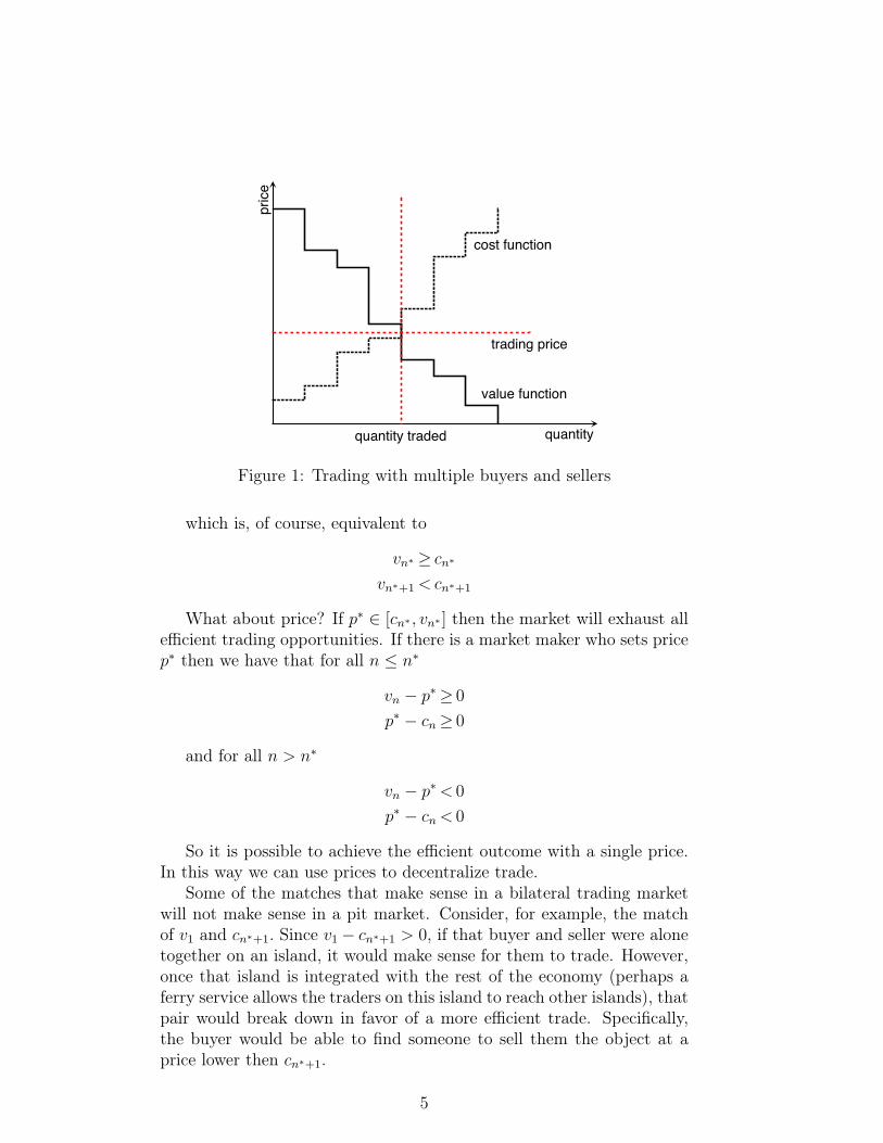
Very simply, this axiom imposes some level of consistency on choices.For example, suppose there were three potential travel locations, Tokyo(T), Beijing (B), and Seoul (S). If a decision maker, when offered thechoice between Tokyo and Beijing chose to go to Tokyo, and when giventhe choice between Beijing and Seoul choose to go to Beijing, then thisaxiom simply says that if they were offered a choice between a trip toTokyo or a trip to Seoul, they would choose Tokyo. This is becausethey have already demonstrated that they prefer Tokyo to Beijing, andBeijing to Seoul, so preferring Seoul to Tokyo would mean that theirpreferences are inconsistent.

7

good 1

good

2

bundle xbundles preferred to b

bundle b

Figure 2: Indifference curve

Axiom 2.3. Reflexivity. For all x ∈ X, x % x (equivalently, x ∼ x).

The final axiom is made for technical reasons, and simply says thata bundle cannot be strictly preferred to itself. Such preferences wouldnot make sense.

These three axioms allow for bundles to be ordered in terms of pref-erence. In fact, these three conditions are sufficient to allow preferencesto be represented by a utility function.

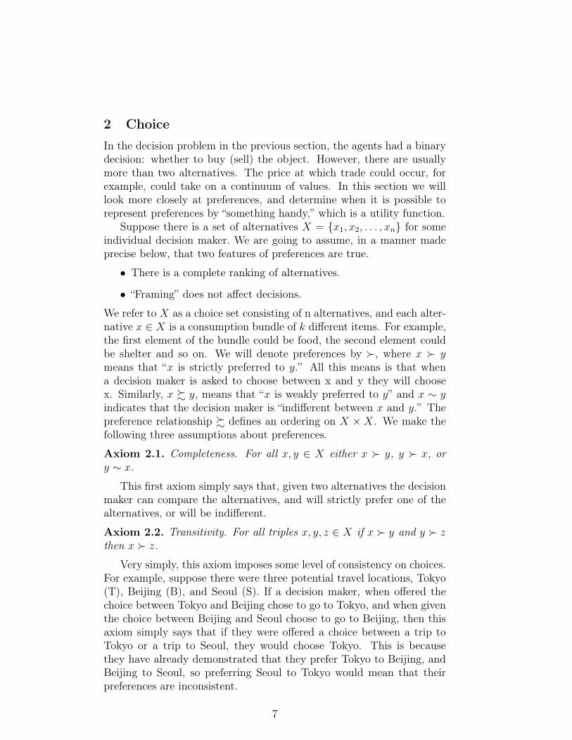
Before elaborating on this, we consider an example. Suppose thereare two goods, Wine and Cheese. Suppose there are four consumptionbundles z = (2, 2), y = (1, 1), a = (2, 1), b = (1, 2) where the two ele-ments of the vector represent the amount of wine or cheese. Most likely,z � y since it provides more of everything (i.e., wine and cheese are“goods”). It is not clear how to compare a and b. What we can do isconsider which bundles are indifferent with b. This is an indifferencecurve (see Figure 2). We can define it as

Ib = {x ∈ X|b ∼ x)

We can then (if we assume that more is better) compare a and b byconsidering which side of the indifference curve a lies on: bundles aboveand to the right are more preferred, bundles below and to the left areless preferred. This reduces the dimensionality of the problem. We canspeak of the “better than b” set as the set of points weakly preferred tob. These preferences are “ordinal:” we can ask whether x is in the betterthan set, but this does not tell us how much x is preferred to b. It iscommon to assume that preferences are monotone: more of a good isbetter.

8

good 1

good

2y

y'

ay+(1-a)y'

Figure 3: Convex preferences

Definition 2.4. The preferences % are said to be (strictly) monotone ifx ≥ y ⇒ x % y (x ≥ y, x 6= y ⇒ x % y for strict monotonicity).1

Suppose I want to increase my consumption of good 1 without chang-ing my level of well-being. The amount I must change x2 to keep utilityconstant, dx2

dx1is the marginal rate of substitution. Most of the time we

believe that individuals like moderation. This desire for moderation isreflected in convex preferences. A mixture between two bundles, be-tween which the agent is indifferent, is strictly preferred to either of theinitial bundle (see Figure 3).

Definition 2.5. A preference relation is convex if for all y and y′ withy ∼ y′ and all α ∈ [0, 1] we have that αy + (1− α)y′ % y ∼ y′.

While convex preferences are usually assumed, there could be in-stances where preferences are not convex. For example, there could bereturns to scale for some good.

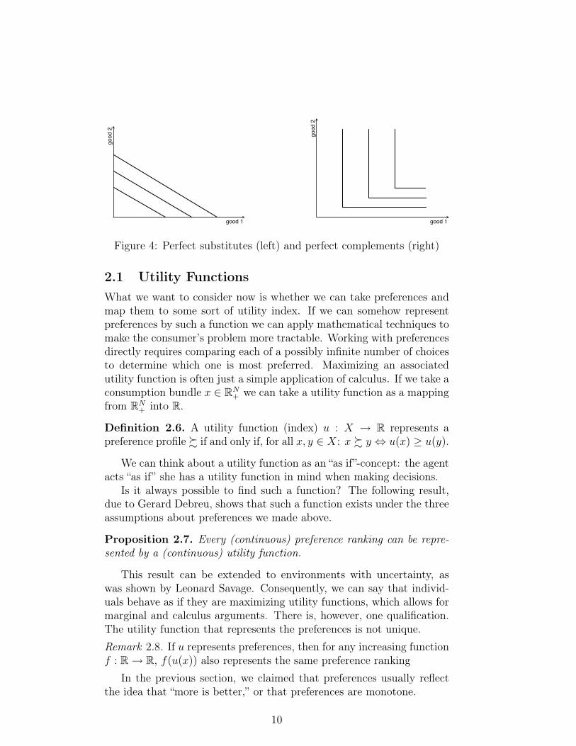
Examples: perfect substitutes, perfect complements (see Figure 4).Both of these preferences are convex.

Notice that indifference curves cannot intersect. If they did we couldtake two points x and y, both to the right of the indifference curve theother lies on. We would then have x � y � x, but then by transitivityx � x which contradicts reflexivity. So every bundle is associated withone, and only one, welfare level.

1If x = (x1, . . . , xN ) and y = (y1, . . . , yN ) are vectors of the same dimension, thenx ≥ y if and only if, for all i, xi ≥ yi. x 6= y means that xi 6= yi for at least one i.

9

good 1

good

2

good 1

good

2

Figure 4: Perfect substitutes (left) and perfect complements (right)

2.1 Utility FunctionsWhat we want to consider now is whether we can take preferences andmap them to some sort of utility index. If we can somehow representpreferences by such a function we can apply mathematical techniques tomake the consumer’s problem more tractable. Working with preferencesdirectly requires comparing each of a possibly infinite number of choicesto determine which one is most preferred. Maximizing an associatedutility function is often just a simple application of calculus. If we take aconsumption bundle x ∈ RN

+ we can take a utility function as a mappingfrom RN

+ into R.

Definition 2.6. A utility function (index) u : X → R represents apreference profile % if and only if, for all x, y ∈ X: x % y ⇔ u(x) ≥ u(y).

We can think about a utility function as an “as if”-concept: the agentacts “as if” she has a utility function in mind when making decisions.

Is it always possible to find such a function? The following result,due to Gerard Debreu, shows that such a function exists under the threeassumptions about preferences we made above.

Proposition 2.7. Every (continuous) preference ranking can be repre-sented by a (continuous) utility function.

This result can be extended to environments with uncertainty, aswas shown by Leonard Savage. Consequently, we can say that individ-uals behave as if they are maximizing utility functions, which allows formarginal and calculus arguments. There is, however, one qualification.The utility function that represents the preferences is not unique.Remark 2.8. If u represents preferences, then for any increasing functionf : R→ R, f(u(x)) also represents the same preference ranking

In the previous section, we claimed that preferences usually reflectthe idea that “more is better,” or that preferences are monotone.

10

Definition 2.9. The utility function (preferences) are monotone increas-ing if x ≥ y implies that u(x) ≥ u(y) and x > y implies that u(x) > u(y).

One feature that monotone preferences rule out is (local) satiation,where one point is preferred to all other points nearby. For economicsthe relevant decision is maximizing utility subject to limited resources.This leads us to consider constrained optimization.

2.2 Budget ConstraintsA budget constraint is a constraint on how much money (income, wealth)an agent can spend on goods. We denote the amount of available incomeby M ≥ 0. x1, . . . , xN are the quantities of the goods purchased andp1, . . . , pN are the according prices. Then the budget constraint is

N∑i=1

pixi ≤M .

As an example, we consider the case with two goods. With monotonepreferences we get that p1x1 +p2x2 = M , i.e., the agent spends her entireincome on the two goods. The points where the budget line intersectswith the axes are x1 = M/p1 and x2 = M/p2 since these are the pointswhere the agent spends her income on only one good. Solving for x2, wecan express the budget line as a function of x1:

x2(x1) =M

p2

− p1

p2

x1,

where dx2

dx1= −p1

p2is the slope of the budget line.

11

good 1

good

2

budget set

optimal choice

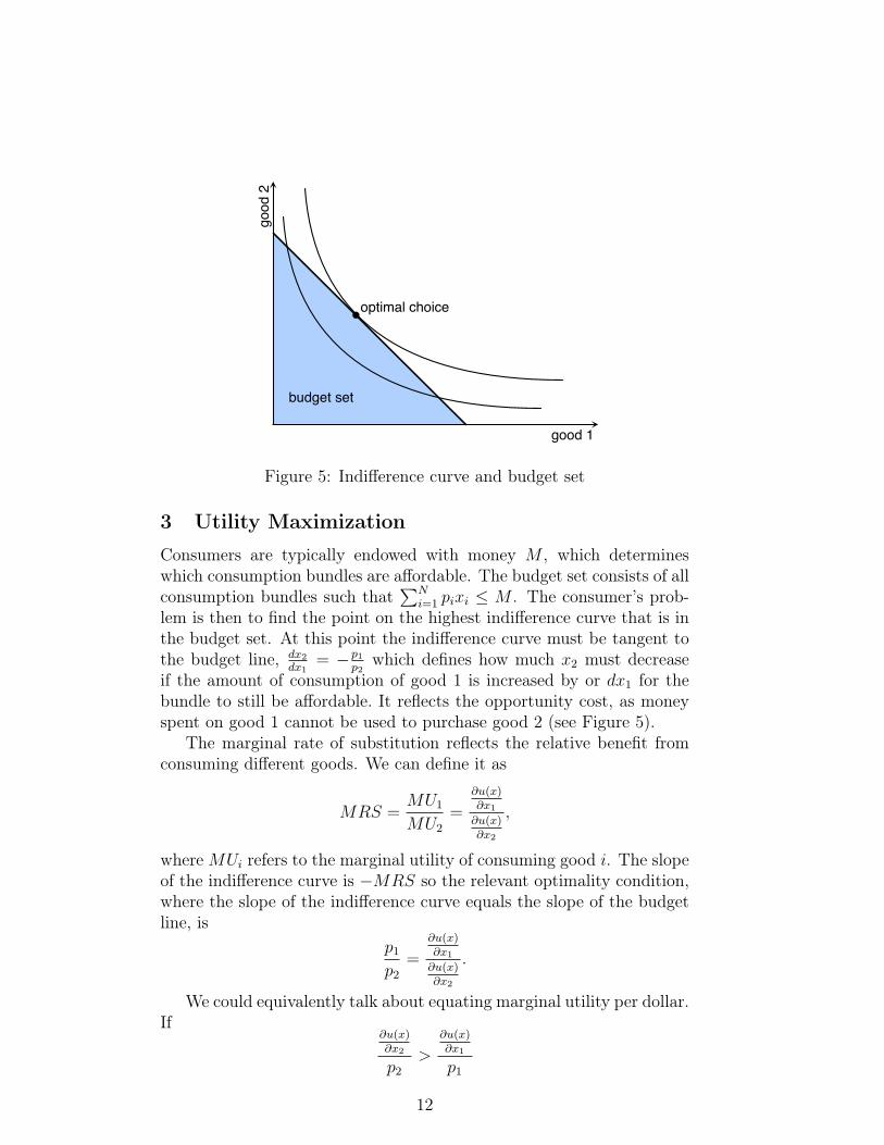
Figure 5: Indifference curve and budget set

3 Utility Maximization

Consumers are typically endowed with money M , which determineswhich consumption bundles are affordable. The budget set consists of allconsumption bundles such that

∑Ni=1 pixi ≤ M . The consumer’s prob-

lem is then to find the point on the highest indifference curve that is inthe budget set. At this point the indifference curve must be tangent tothe budget line, dx2

dx1= −p1

p2which defines how much x2 must decrease

if the amount of consumption of good 1 is increased by or dx1 for thebundle to still be affordable. It reflects the opportunity cost, as moneyspent on good 1 cannot be used to purchase good 2 (see Figure 5).

The marginal rate of substitution reflects the relative benefit fromconsuming different goods. We can define it as

MRS =MU1

MU2

=

∂u(x)∂x1

∂u(x)∂x2

,

whereMUi refers to the marginal utility of consuming good i. The slopeof the indifference curve is −MRS so the relevant optimality condition,where the slope of the indifference curve equals the slope of the budgetline, is

p1

p2

=

∂u(x)∂x1

∂u(x)∂x2

.

We could equivalently talk about equating marginal utility per dollar.If

∂u(x)∂x2

p2

>

∂u(x)∂x1

p1

12

then one dollar spent on good 2 generates more utility then one dollarspent on good 1. So shifting consumption from good 1 to good 2 wouldresult in higher utility. So, to be at an optimum we must have themarginal utility per dollar equated across goods.

Does this mean then that we must have ∂u(x)∂xi

= pi at the optimum?No. Such a condition wouldn’t make sense since we could rescale theutility function. We could instead rescale the equation by a factor λ ≥ 0that converts “money” into “utility.” We could then write ∂u(x)

∂xi= λpi.

Here, λ reflects the marginal utility of money.

3.1 Optimization by SubstitutionThe consumer’s problem is to maximize utility subject to a budgetconstraint. There are two ways to approach this problem. The firstapproach involves writing the last good as a function of the previousgoods, and then proceeding with an unconstrained maximization. Con-sider the two good case. The budget set consists of the constraint thatp1x1 + p2x2 ≤M . So the problem is

maxx1,x2

u(x1, x2) subject to p1x1 + p2x2 ≤M

But notice that whenever u is (locally) non-satiated then the budgetconstraint holds with equality since there in no reason to hold moneythat could have been used for additional valued consumption. So, p1x1 +p2x2 = M , and so we can solve for x2 = M−p1x1

p2. Now we can maximize

u(x1,

M−p1x1

p2

)as the standard single variable maximization problem.

Example 3.1. We consider a consumer with Cobb-Douglas preferences.Cobb-Douglas preferences are easy to use and therefore commonly used.The utility function is defined as (with two goods)

u(x1, x2) = xα1x1−α2 , α > 0

The goods’ prices are p1,p2 and the consumer if endowed with incomeM . Hence, the constraint optimization problem is

maxx1,x2

xα1x1−α2 subject to p1x1 + p2x2 = M .

We solve this maximization by substituting the budget constraintinto the utility function so that the problem becomes an unconstrainedoptimization with one choice variable:

u(x1) = xα1

(M − p1x1

p2

)1−α

. (1)

13

In general, we take the total derivative of the utility function

du(x1, x2(x1))

dx1

=∂u

∂x1

+∂u

∂x2

dx2

dx1

= 0

which gives us the condition for optimal demand

dx2

dx1

= −∂u∂x1

∂u∂x2

.

The right-hand side is the marginal rate of substitution (MRS).In order to calculate the demand for both goods, we go back to our

example. Taking the derivative of the utility function (1)

u′(x1) = αxα−11

(M − p1x1

p2

)1−α

+ (1− α)xα1

(M − p1x1

p2

)−α(−p1

p2

)= xα−1

1

(M − p1x1

p2

)−α [αM − p1x1

p2

− (1− α)x1p1

p2

]so the FOC is satisfied when

α(M − p1x1)− (1− α)x1p1 = 0

which holds whenx∗1 =

αM

p1

. (2)

Hence, we see that the budget spent on good 1, p1x1, equals the budgetshare αM , where α is the preference parameter associated with good 1.

Plugging (2) into the budget constraint yields

x∗2 =M − p1x1

p2

=(1− α)M

p2

.

Several important features of this example are worth noting. First ofall, x1 does not depend on p2 and vice versa. Also, the share of incomespent on each good pixi

Mdoes not depend on price or wealth. What is

going on here? When the price of one good, p2, increases there are twoeffects. First, the price increase makes good 1 relatively cheaper (p1

p2de-

creases). This will cause consumers to “substitute” toward the relativelycheaper good. There is also another effect. When the price increasesthe individual becomes poorer in real terms, as the set of affordable con-sumption bundles becomes strictly smaller. The Cobb-Douglas utilityfunction is a special case where this “income effect” exactly cancels outthe substitution effect, so the consumption of one good is independentof the price of the other goods.

14

3.2 Optimization Using the Lagrange ApproachWhile the approach using substitution is simple enough, there are sit-uations where it will be difficult to apply. The procedure requires thatwe know, before the calculation, that the budget constraint actuallybinds. In many situations there may be other constraints (such as a non-negativity constraint on the consumption of each good) and we may notknow whether they bind before demands are calculated. Consequently,we will consider a more general approach of Lagrange multipliers. Again,we consider the (two good) problem of

maxx1,x2

u(x1, x2) s.t. p1x1 + p2x2 ≤M

Let’s think about this problem as a game. The first player, let’scall him the kid, wants to maximize his utility, u(x1, x2), whereas theother player (the parent) is concerned that the kid violates the budgetconstraint, p1x1 + p2x2 ≤ M , by spending too much on goods 1 and2. In order to induce the kid to stay within the budget constraint, theparent can punish him by an amount λ for every dollar the kid exceedshis income. Hence, the total punishment is

λ(M − p1x1 − p2x2).

Adding the kid’s utility from consumption and the punishment, we get

L(x1, x2, λ) = u(x1, x2) + λ(M − p1x1 − p2x2). (3)

Since, for any function, we have max f = −min f , this game is a zero-sum game: the payoff for the kid is L and the parent’s payoff is −L sothat the total payoff will always be 0. Now, the kid maximizes expression(3) by choosing optimal levels of x1 and x2, whereas the parent minimizes(3) by choosing an optimal level of λ:

minλ

maxx1,x2

L(x1, x2, λ) = u(x1, x2) + λ(M − p1x1 − p2x2).

In equilibrium, the optimally chosen level of consumption, x∗, hasto be the best response to the optimal level of λ∗ and vice versa. Inother words, when we fix a level of x∗, the parent chooses an optimalλ∗and when we fix a level of λ∗, the kid chooses an optimal x∗. Inequilibrium, no one wants to deviate from their optimal choice. Could itbe an equilibrium for the parent to choose a very large λ? No, becausethen the kid would not spend any money on consumption, but ratherhave the maximized expression (3) to equal λM .

15

Since the first-order conditions for minima and maxima are the same,we have the following first-order conditions for problem (3):

∂L∂x1

=∂u

∂x1

− λp1 = 0 (4)

∂L∂x2

=∂u

∂x2

− λp2 = 0 (5)

∂L∂λ

= M − p1x1 − p2x2 = 0.

Here, we have three equations in three unknowns that we can solve forthe optimal choice x∗, λ∗.

Before solving this problem for an example, we can think about itin more formal terms. The basic idea is as follows: Just as a neces-sary condition for a maximum in a one variable maximization problemis that the derivative equals 0 (f ′(x) = 0), a necessary condition for amaximum in multiple variables is that all partial derivatives are equal to0 (∂f(x)

∂xi= 0). To see why, recall that the partial derivative reflects the

change as xi increases and the other variables are all held constant. Ifany partial derivative was positive, then holding all other variables con-stant while increasing xi will increase the objective function (similarly,if the partial derivative is negative we could decrease xi). We also needto ensure that the solution is in the budget set, which typically won’thappen if we just try to maximize u. Basically, we impose a “cost” onconsumption (the punishment in the game above), proceed with uncon-strained maximization for the induced problem, and set this cost so thatthe maximum lies in the budget set.

Notice that the first-order conditions (4) and (5) imply that

∂u∂x1

p1

= λ =∂u∂x2

p2

or∂u∂x1

∂u∂x2

=p1

p2

which is precisely the “MRS = price ratio” condition for optimality thatwe saw before.

Finally, it should be noted that the FOCs are necessary for opti-mality, but they are not, in general, sufficient for the solution to bea maximum. However, whenever u(x) is a concave function the FOCsare also sufficient to ensure that the solution is a maximum. In mostsituations, the utility function will be concave.

16

Example 3.2. We can consider the problem of deriving demands for aCobb-Douglas utility function using the Lagrange approach. The asso-ciated Lagrangian is

L(x1, x2, λ) = xα1x1−α2 + λ(M − p1x1 − p2x2),

which yields the associated FOCs

∂L∂x1

= αxα−11 x1−α

2 − λp1 = α

(x2

x1

)1−α

− λp1 = 0 (6)

∂L∂x2

= (1− α)xα1x−α2 − λp2 = (1− α)

(x1

x2

)α− λp2 = 0 (7)

λ(M − p1x1 − p2x2) = 0. (8)

We have three equations with three unknowns (x1, x2, λ) so that thissystem should be solvable. Notice that since it is not possible that x2

x1

and x1

x2are both 0 we cannot have a solution to equations (6) and (7)

with λ = 0. Consequently we must have that p1x1 + p2x2 = M in orderto satisfy equation (8). Solving for λ in the above equations tells us that

λ =α

p1

(x2

x1

)1−α

=(1− α)

p2

(x1

x2

)αand so

p2x2 =1− αα

p1x1.

Combining with the budget constraint this gives

p1x1 +1− αα

p1x1 =1

αp1x1 = M .

So the Marshallian2 demand functions are

x∗1 =αM

p1

andx∗2 =

(1− α)M

p2

.

So we see that the result of the Lagrangian approach is the same as fromapproach that uses substitution. Using equation (6) or (7) again alongwith the optimal demand x∗1 or x∗2 gives us the following expression forλ:

λ∗ =1

M.

Hence, λ∗ equals the derivative of the Lagrangian L with respect toincome M . We call this derivative, ∂L

∂M, the marginal utility of money.

2After the British economist Alfred Marshall.

17

When we take a monotone transformation of a utility function theunderlying preferences represented are not changed. Consequently theconsumer’s demands are unaffected by such a transformation. The fol-lowing example shows this using a monotone transformation of the Cobb-Douglas utility function.

Example 3.3. Notice that

ln(xα1x

1−α2

)= α lnx1 + (1− α) lnx2

so we could write the utility function for Cobb-Douglas preferences byu(x1, x2) = α lnx1 + (1− α) lnx2. The associated Lagrangian is

L(x1, x2, λ) = α lnx1 + (1− α) lnx2 + λ(M − p1x1 − p2x2)

with associated FOCs∂L∂x1

=α

x1

− λp1 = 0

∂L∂x2

=1− αx2

− λp2 = 0

λ(M − p1x1 − p2x2) = 0.

Since αx1> 0 we must have λ > 0 so the budget constraint must hold

with equality. Solving for λ gives

λ =α

p1x1

=1− αp2x2

sop2x2 =

1− αα

p1x1.

and1− αα

p1x1 + p1x1 =1

αp1x1 = M .

So, we can conclude, as in the previous example, that

x1 =αM

p1

andx2 =

(1− α)M

p2

.

After we calculate the optimal choice (or Marshallian demand func-tions), we can plug them into the original utility function to get theindirect utility function, which is a function of prices and income only:

V (p1, p2,M) = u (x∗1(p1, p2,M), x∗2(p1, p2,M)) .

It turns out that ∂V∂M

= λ∗ = ∂L∂M

, which is therefore also called themarginal value of income.

18

50 1 2 3 4

5

0

1

2

3

4

good 1

good

2

budget line

slope = 2

indifference curve

Figure 6: Leontief preferences

4 Demand

So far we have considered only the decisions of single agents trying tomake the optimal decisions given some exogenous parameters and con-straints. In the next sections we will integrate these individual decisionmakers with other decision makers and consider when the resulting sys-tem is in “equilibrium.” First, we will consider the behaviour of demands.

4.1 Comparative StaticsAfter having derived the optimal demand functions x∗1(p1, p2,M) andx∗2(p1, p2,M) we can ask how a change in the exogenous variables (p1,p2, and M) affects the endogenous variables (x and y). This exercise isknown as comparative statics. For example, a firm might be interestedin how its revenue pixi changes when it increases the price of its good,pi.

Example 4.1. Consider the following utility function, also known asLeontief utility:3

u(x1, x2) = min {2x1, x2} .

A consumer with this type of utility function only achieves a higherutility level when the quantity of both goods increases. An example isleft and right shoes: many left shoes do not increase utility unless theyare matched by the same number of right shoes. The indifference curvesfor the utility function are depicted in Figure 6. The utility maximization

3After Wassily Leontief, a Russian economist, sought after in vain by the CIA,who used this functional form in his analysis of production technology and growth.

19

problem ismaxx1,x2

min {2x1, x2} s.t. p1x1 + p2x2 = M . (9)

Looking at the indifference curves, we see that optimal consumptionbundles satisfy the condition 2x1 = x2, i.e., optimal bundles are locatedat the kinks of the indifference curves. Starting at one of the kinks,consuming more of good 1 or more of good 2 does not increase utility.Hence we can find the solution to problem (9) as the intersection ofthe line 2x1 = x2 with the budget line. We solve by substituting theoptimality condition into the budget constraint:

p1x1 + p2(2x1) = M.

Hence, the optimal demand functions are

x∗1(p1, p2,M) =M

p1 + 2p2

and, by plugging x∗1 into the optimality condition,

x∗2(p1, p2,M) =2M

p1 + 2p2

.

Note that we cannot equate the MRS with the slope of the budget linehere, because the MRS is not defined at the point where 2x1 = x2.Next, we do comparative statics by taking the derivative of the en-dogenous variables with respect to the exogenous variables (using thequotient rule for derivatives):

∂x∗1∂p1

= − M

(p1 + 2p2)2< 0,

which is called the own-price effect on demand, and

∂x∗1∂p2

= − 2M

(p1 + 2p2)2< 0,

which is the cross-price effect on demand. Note that the demand forgood 1 decreases when p1 increases and when p2 increases.

In general, we say that goods i and j are substitutes if the cross-priceeffect is positive, i.e., demand for good i increases when the price of goodj increases:

∂x∗i∂pj≥ 0

20

and they are called complements if the cross-price effect is negative:

∂x∗i∂pj

< 0.

Hence, in the Leontief example, the two goods are complements. Infact, they are called perfect complements in this case. Besides the priceeffects, we can also calculate the income effect, which is defined as

∂x∗i∂M

≷ 0.

4.2 ElasticitiesWhen calculating price effects, the result depends on the units used. Forexample, when considering the own-price effect for gasoline, we mightexpress quantity demanded in gallons or liters and the price in dollarsor euros. The own-price effects would differ even if consumers in theU.S. and Europe had the same underlying preferences. In order to makeprice effects comparable across different units, we can normalize them bydividing by xi

pi. This is the own-price elasticity of demand and denoted

by ε:

ε = −∂xi

∂pi

xi

pi

= −∂xi∂pi

pixi.

It is common to multiply the price effect by −1 so that ε is a positivenumber since the price effect is usually negative. Of course, the cross-price elasticity of demand is defined similarly

−∂xi

∂pj

xi

pj

= −∂xi∂pj

pjxi.

Price elasticities measure by how many percent demand changes in re-sponse to a one percent change in price.

Price elasticities play an important role in economics. Consider afirm trying to maximize the revenue generated by demand for its good.Revenue is the product of quantity demanded and price:

R = xi(p)pi.

The firm chooses the price of its good, pi, in order to maximize R. Theeffect of price on revenue is, using the chain rule:

dR

dpi= xi(p) +

dxidpi

pi.

21

Factoring out xi(p) we can rewrite this as

dR

dpi= xi(p)

[1 +

dxidpi

pix1(p)

]= xi(p) (1− ε) .

Hence, the effect of price on revenue depends on the own-price elasticityof demand. We have that

dR

dpi

> 0 if ε < 1

= 0 if ε = 1

< 0 if ε > 1

.

In the first case, demand is called inelastic, in the second case, it has unitelasticity, and in the third case, it is called elastic. Intuitively, price hastwo effects on revenue: a higher price increases revenue since the latter isthe product of quantity and price, but a higher price also decreases thequantity demanded as long as the own-price effect is negative. Hence,the elasticity measures which of the two opposite effects dominates.

4.3 Income and Substitution Effects, ExpenditureMinimization

For given prices and wealth an individual has demands (x∗1(p1, p2,M),x∗2(p1, p2,M)). As we’ve seen above, the demand for good 1 can be af-fected by changes in its own price, ∂x1

∂p1, or by a cross-price effect ∂x1

∂p2.

When the price of good 2 changes there are two effects. First, itmakes the prices ratio p1

p2change. This is known as the substitution effect.

Second, the change in p2 causes a change in the consumption bundlesthat are feasible, so an increase in p2 makes the consumer poorer, whilea decrease makes individuals richer. This effect is known as the incomeeffect. Together these two effects constitute a price effect.

Example 4.2. One example where the substitution effect does not mat-ter is the Leontieff utility function. Goods are perfect complements andso there is no substitution. Here, u(x) = min{ax1, bx2} so it will beoptimal to set ax1 = bx2 whatever the prices of the two goods may be.So x2 = ax1

band from the budget set p1x1 + p2x2 =

(p1 + ap2

b

)x1 = M .

So

x1 =bM

bp1 + ap2

x2 =aM

bp1 + ap2

If the price of good 1 were to fall the consumption of both goods willincrease, since the consumer is made wealthier (more bundles are nowaffordable).

22

Now we express income and substitution effects analytically. To doso, we introduce expenditure minimization first. Recall the general util-ity maximization problem from section 3. With many goods and priceswe can write it as (writing x and p are vectors with I components each)

maxx

u(x) s.t. p · x ≤M.

The resulting demand function is denoted by x∗(p,M) and also calleduncompensated demand or Marshallian demand. Plugging in the optimaldemand into the utility function yields indirect utility as a function ofprices and income:

V (p,M) = u(x∗(p,M)).

Instead of maximizing utility subject to a given income we can alsominimize expenditure subject to achieving a given level of utility u. Inthis case, the consumer wants to spend as little money as possible toenjoy a certain utility. Formally, we write

minx

p · x s.t. u(x) ≥ u. (10)

The result of this optimization problem is a demand function again, butin general it is different from x∗(p,M). We call the demand functionderived from problem (10) compensated demand or Hicksian demand4

and denote it by xc(p, u). Note that compensated demand is a function ofprices and the utility level whereas uncompensated demand is a functionof prices and income. Plugging compensated demand into the objectivefunction (p · x) yields the expenditure function as function of prices andu

E(p, u) = p · xc(p, u).

Hence, the expenditure measures the minimal amount of money requiredto buy a bundle that yields a utility of u.

Uncompensated and compensated demand functions usually differfrom each other, which is immediately clear from the fact that theydifferent arguments. There is a special case where they are identical.First, note that indirect utility and expenditure function are related bythe following relationships

V (p, E(p, u)) = u

E(p, V (p,M)) = M.

That is, if income is exactly equal to the expenditure necessary to achieveutility level u, then the resulting indirect utility is equal to u. Similarly, if

4After the British economist Sir John Hicks, co-recipient of the 1972 Nobel Prizein Economic Sciences.

23

the required utility level is set equal to the indirect function when incomeis M , then minimized expenditure will be equal to M . Using theserelationships, we have that uncompensated and compensated demandare equal in the following two cases:

x∗(p,M) = xc(p, V (p,M))

x∗(p, E(p, u)) = xc(p, u). (11)

Now we can express income and substitution effects analytically.Start with one component of equation (11) (recall that x and p arevectors):

xci(p, u) = x∗i (p, E(p, u))

and take the derivative with respect to pj using the chain rule

∂xci∂pj

=∂x∗i∂pj

+∂x∗i∂M

∂E

∂pj. (12)

Now we have to find an expression for ∂E∂pj

. Start with the Lagrangianassociated with problem (10) evaluated at the optimal solution (xc(p, u),λ∗(p, u)):

L(xc(p, u), λ∗(p, u)) = p · xc(p, u) + λ∗(p, u)[u− u(x(p, u))].

Taking the derivative with respect to any price pj and noting that u =u(x(p, u)) at the optimum we get

∂L(xc(p, u), λ∗(p, u))

∂pj=xcj +

I∑i=1

pi∂xci∂pj− λ∗

I∑i=1

∂u

∂xi

∂xi∂pj

=xcj +I∑i=1

(pi − λ∗

∂u

∂xi

)∂xi∂pj

.

But the first -order conditions for this Lagrangian are

pi − λ∂u

∂xi= 0 for all i.

Hence∂E

∂pj=∂L∂pj

= xcj(p, u).

This result also follows form the Envelope Theorem. Moreover, fromequation (11) it follows that xcj = x∗j . Hence, using these two facts and

24

bringing the second term on the RHS to the LHS we can rewrite equation(12) as

∂x∗i∂pj

=∂xci∂pj︸︷︷︸SE

− x∗j∂x∗i∂M︸︷︷︸IE

.

This equation is known as the Slutsky Equation5 and shows formallythat the price effect can be separated into a substitution (SE) and anincome effect (IE).

4.4 Corner SolutionsConsider the utility function u(x1, x2) = ln x1 + x2, where p1, p2 and Mare all strictly greater than 0. The first thing to notice is that while themarginal utility of good 2 is constant ∂u

∂x2= 1, the marginal utility of

good 1, ∂u∂x1

= 1x1

is a decreasing function of x1. The second derivativeis negative, ∂2u

∂x21

= − 1x21< 0 because the natural logarithm is a concave

function. That is, there is diminishing marginal utility from consuminggood 1. Suppose that we consider the problem of maximizing u(x) =lnx1 +x2 subject to the budget constraint, p1x1 + p2x2 ≤M . We wouldexpect that the size of the budget would greatly affect the shape of thedemands. The consumer will spend everything on good 1 as long as

MU1

p1

≥ MU2

p2

.

Once x1 is large enough thatMU1

p1

=MU2

p2

we reach a “critical point” and it becomes more profitable to spend theremaining money on good 2. This point occurs when

1x1

p1

=1

p2

So x∗1 = p2p1. Hence, the first p1x

∗1 dollars will be spent on good 1, and any

remaining money will be spent on good 2. The maximum amount tobe spent on good 1 is simply m∗ = p1x

∗1 = p2. So we can now formulate

the demand. {x1 = M

p1

x2 = 0

}ifM <m∗ = p2{

x1 = p2p1

x2 = M−p2p1

}ifM ≥m∗ = p2

5After the Russian statistician and economist Eugen Slutsky.

25

In the above example, with a small budget it would be preferableto consume negative amounts of good 2. This negative consumption iscalled “short selling.” In most situations this is not reasonable. Whatwould it mean, for example, to consume −2 apples? Consequently, weoften need to add additional constraints to the problem: that the con-sumption of each good must be non-negative. When such constraintsbind we have what is known as a “corner solution.” We can deal withthese non-negativity constraints exactly the same way as the budget con-straint: by adding Lagrange multipliers associated with each constraint.Unlike with the budget constraint which will hold with equality when-ever utility functions are monotone, it may not be clear before beginningthe calculation which non-negativity constraint will bind. Instead of justhaving the budget constraint

p1x1 + p2x2 ≤M

we also have the constraints

x1≥ 0

x2≥ 0.

Typically the Lagrange multipliers associated with these constraints aredenoted by µ1 and µ2.

So the associated Lagrangian is

L(x1, x2, λ, µ1, µ2) = u(x1, x2) + λ(M − p1x1 − p2x2) + µ1x1 + µ2x2.

Note that the Lagrangian has 5 arguments now (2 goods and 3 multi-pliers). This leads to the following FOCs:

∂L∂x1

=∂u

∂x1

− λp1 + µ1 = 0

∂L∂x2

=∂u

∂x2

− λp2 + µ2 = 0

and the complimentary slackness conditions (see section 5.5 for more onthis)

λ(M − p1x1 − p2x2) = 0 (13)µ1x1 = 0 (14)µ2x2 = 0. (15)

This means we are left with 5 equations in 5 unknowns. In theprevious example with u(x1, x2) = lnx1 + x2, the first two conditions

26

become

1

x1

− λp1 + µ1 = 0 (16)

1− λp2 + µ2 = 0. (17)

For small M , x1 > 0 we have that x2 = 0 and so µ1 = 0 for condition(14) to hold. But the budget constraint (13) guarantees that

x1 =M

p1

which combined with condition (16) says that λ = 1M. So, from condition

(17)µ2 =

p2

M− 1

This is the shadow price of short-selling. That is, how valuable relaxingthe non-negativity constraint on good 2 would be.

27

5 A Brief Review of Optimization

Let us start with a function on the real line

f : R→ R

which is continuous and differentiable. We want to identify local andglobal maxima in a world without constraints, i.e., we are looking atunconstrained optimization:

maxx∈R

f (x)

x∗ is a global maximum if

for all x, f(x∗) ≥ f(x).

The necessary conditions for a local or a global maximum at x = x∗ aregiven by the first order condition (FOC):

f ′ (x∗) = 0,

and the second order condition

f ′′ (x∗) ≤ 0.

A sufficient condition for a global maximum is given by

f ′ (x∗) = 0,

and here comes the new part for the sufficiency condition

for all x, f ′′ (x) ≤ 0.

Definition 5.1. A univariate function f : R→ R is a concave functionif u′′(x) < 0.

A concave function has only a single (global) maximum and no min-imum.

5.1 ConstraintsWe consider again a continuous and differentiable function

f : R→ R

but now impose constraints on the function, or on the search

x ∈ [−∞, x]

28

for some x < x. In other words we are looking for

max f (x)

subject tox− x ≥ 0

The inequalities represent the constraint which simply say that we canlook for the x which maximizes f (x) but only in the range of the interval[−∞, x].

If the optimal x∗ = x, then we say that x∗ is a corner solution.It is easy to see that a corner solution may not satisfy the first ordercondition:

f ′ (x∗) = 0,

because the decision maker would like to move his choice in a directionwith a positive gradient but the constraint does not allow him to gobeyond x. For example if x∗ = x, then we might have at x = x∗ :

f ′ (x∗) ≥ 0.

We now would like to introduce a general method so that the first orderconditions, namely the idea that there are no further net gains to bemade, is reestablished. Second we would like to integrate the constraintsdirectly in the objective function so that the problem becomes to lookmore like an unconstrained problem, and hence more familiar with us.Finally, we would like to reinterpret the role of constraint in terms of aprice.

5.2 LagrangeJoseph-Louis Lagrange, comte de l’Empire (January 25, 1736 – April 10,1813) was an Italian-French mathematician and astronomer who madeimportant contributions to all fields of analysis and number theory andto classical and celestial mechanics as arguably the greatest mathemati-cian of the 18th century. It is said that he was able to write out hispapers complete without a single correction required. Before the age of20 he was professor of geometry at the royal artillery school at Turin. Byhis mid-twenties he was recognized as one of the greatest living math-ematicians because of his papers on wave propagation and the maximaand minima of curves.

He was born, of French and Italian descent, in Turin. His father,who had charge of the Kingdom of Sardinia’s military chest, was ofgood social position and wealthy, but before his son grew up he hadlost most of his property in speculations, and young Lagrange had to

29

rely on his own abilities for his position. He was educated at the collegeof Turin, but it was not until he was seventeen that he showed anytaste for mathematics – his interest in the subject being first excited bya paper by Edmund Halley which he came across by accident. Aloneand unaided he threw himself into mathematical studies; at the end ofa year’s incessant toil he was already an accomplished mathematician,and was made a lecturer in the artillery school.

In mathematical optimization problems, Lagrange multipliers, namedafter Joseph Louis Lagrange, is a method for finding the local extremaof a function of several variables subject to one or more constraints.This method reduces a problem in n variables with k constraints to asolvable problem in n + k variables with no constraints. The methodintroduces a new unknown scalar variable, the Lagrange multiplier, foreach constraint and forms a linear combination involving the multipliersas coefficients.

5.3 Constrained OptimizationWe are looking for a solution of the following problem

maxx∈R

f (x)

subject tox− x ≥ 0.

We approach this problem by associating a Lagrange multiplier to theconstraint, and it is typically a Greek letter, say λ ∈ R+, and define afunction on x and λ, called the Lagrangian function, L:

L (x, λ) = f (x) + λ (x− x) .

We now have a new function, in two (x, λ) rather than one (x) variable.We impose the following constraint on the shape of the Lagrangian

λ (x− x) = 0 (18)

for all x and all λ. The new constraint, (18), is often called the comple-mentary slackness constraint. We now maximize the Lagrange an withrespect to x (and as it turns out also minimize it with respect to λ):

maxxL (x, λ) .

We now look at the first order conditions of the unconstrained problemand find the first order condition

f ′ (x∗)− λx∗ = 0

30

and the auxiliary complementary slackness constraint:

λ (x− x∗) = 0.

If x∗ is a corner solution with x∗ = x, then λ ≥ 0 and we can interpretλ as the price (of violating the constraint). In the process we havereplaced the strict constraint with a price for the constraint (equal tothe Lagrange multiplier). At the optimum the price is equal to themarginal value of the objective function. For this reason we refer to itas the shadow price of the constraint. It is the smallest price we canassociate to the constraint so that the decision maker, facing this pricewould respect the constraint.

5.4 ExampleConsider the following function

f (x) = a− (x− b)2

with a, b > 0.

1. Graphically display the function, label a and b on the respectiveaxis. Solve analytically for the unconstrained maximum of thisfunction.

2. Suppose now that the choice of the optimal x is constrained byx ≤ x, where x is an arbitrary number, satisfying

0 < x < b.

(a) Graphically display the nature of the new constraint relativeto the optimization problem and the function f .

(b) Solve via the Lagrangian method for the optimal solution.

(c) Lagrange multiplier. Suppose that we increase the boundx by dx. What is the marginal effect this has on the value ofthe function to be optimized in terms of a and b. How does itcompare to the value of the Lagrangian multiplier which youjust computed.

(d) Interpretation of Lagrangian multiplier. Imagine nowthat we cannot insist that the decision maker respect the con-straint but that we can ask a penalty, say λ, for every unitof x over and above x. What is the price that we would haveto charge so that the decision maker would just be happy toexactly choose x∗ = x and thus in fact respect the constraint

31

even so did not face the constraint directly.In the process we have replaced the strict constraint with aprice for the constraint (equal to the Lagrange multiplier).At the optimum the price is equal to the marginal value ofthe objective function. For this reason we refer to it as theshadow price of the constraint. It is the smallest price we canassociate to the constraint so that the decision maker, facingthis price would respect the constraint.

5.5 Understanding LagrangiansRecall that we can solve the general utility maximization problem byusing the Lagrange approach as follows:

maxx1,x2

minλL(x1, x2, λ),

where the Lagrangian L is defined as

L(x1, x2, λ) = u(x1, x2) + λ(M − p1x1 − p2x2),

so that the resulting problem is an unconstrained optimization problem.Graphically we can interpret this approach as follows: Imagine we canchoose a value of x on the north-south axis to maximize L, i.e., we are“climbing a mountain” along this axis. Along the east-west axis we picka λ to minimize L. The solution to this problem is a “saddle point:”a point that is the lowest (along the east-west axis) among the highestpoint along the north-south axis.

Before we proceed we consider the simplest possible constrained prob-lem, the one-dimensional maximization problem, to develop a feel forhow this technique works. Let f(x) be a function from the real line intoitself (for example the solid black one depicted in Figure 7). The prob-lem is to choose x to maximize f(x). In the unconstrained problem, theFOC f ′(x∗) = 0 is a sufficient condition for a local extremum. To ensurethat said extremum is in fact a local maximum we must consider thesecond-order condition f ′′(x∗) ≤ 0. What if we are interested in a globalmaximum? Then we could replace the above SOC with f ′′(x) ≤ 0 forall x. This will guarantee that the function is concave and so any localmaximum must be a global maximum.

Let x = arg max f(x), and consider some x < x and suppose insteadthat we are considering the problem of maximizing f(x) subject to x ≤ x.Assume that f is concave at x. We know that f ′(x) = 0 but x is notavailable in the new problem. Is there an analogous expression for thesolution to the constrained problem?

32

x

f(x)

x "hat"x "bar"

Figure 7: A one-dimensional maximization problem

If we consider the constrained problem we know that f is increasingat x, so we expect the the solution to be x∗ = x, a “corner solution.” Thatis, although x is the solution to the constrained maximization problem,the FOC is not satisfied at this point: f(x) 6= 0. We can write thisproblem as the associated Lagrangian:

L(x, λ) = f(x)− λ(x− x).

Again, we can interpret λ as a penalty. If x exceeds x by one unitthe objective function L decreases by λ. As before, we maximize theLagrangian with respect to x and minimize with respect to λ:

maxx

minλL(x, λ) = f(x)− λ(x− x).

The first-order conditions are

∂L∂x

= f ′(x)− λ = 0 (19)

∂L∂λ

= x− x = 0 or λ = 0. (20)

The two expressions in equation (20) can also be combined and writtenas

λ (x− x) = 0,

which is known as the complementary slackness condition. In otherwords, either x = x, in which case λ > 0 is necessary as a penalty,or λ = 0, which means that the constraint is not binding so that thereis no need to penalize for exceeding the constraint (for example if we

33

replace part of the solid black function in Figure 7 by the dashed redfragment). Hence, we have to distinguish two cases after determining x∗and λ∗:

x∗ < x⇒ λ∗ = 0

x∗ = x⇒ λ∗ = f ′(x∗).

In both cases, equations (19) and (20) are satisfied.How do we know that we won’t have x∗ > x? Under the original

formulation individuals were simply not allowed to choose a bundle thatviolates the constraint, but under the Lagrangian approach the maxi-mization is unconstrained. The λ term introduces a “price,” that ensuresthat individuals do not choose to consume more then is feasible. If morewas consumed than available then this price would have been set toolow. So rather than setting unbreakable constraints, the economics ap-proach is to allow for “prices” that make individuals not want to chooseimpossible amounts given the resource constraints in the economy. Thisallows for “decentralizing via prices.”

The Lagrange multiplier λ is also called a shadow price or marginalvalue of the constraint. The latter term becomes clear when we con-sider the marginal value of increasing x, i.e., of relaxing the constraint.Suppose we have solved the constraint maximization problem

maxx≤x

f(x)

and derived the optimal values x∗ (x) and λ∗ (x). Then the value of theLagrangian is

L (x∗ (x) , λ∗ (x)) = f (x∗ (x))− λ∗ (x) [x∗ (x)− x] .

Now we can calculate the marginal value of relaxing (i.e., increasing) xby taking the derivative

∂L (x∗ (x) , λ∗ (x))

∂x= f ′ (x∗ (x))x∗′ (x)− λ∗ (x)x∗′ (x) + λ∗ (x) ,

which can be rewritten as

[f ′ (x∗ (x))− λ∗ (x)]x∗′ (x) + λ∗ (x) .

But from equation (19) we know that the term in square brackets isequal to zero. Hence

∂L (x∗ (x) , λ∗ (x))

∂x= λ∗ (x) .

In other words, the marginal value of relaxing the constraint is equal tothe shadow price λ.

34

y

z

λz+(1-λ)y

f(y)

f(z)

f(λz+(1-λ)y)

λf(z)+(1-λ)f(y)

Figure 8: A concave function

5.6 Concavity and Quasi-ConcavityA function f : RN → R is called concave if for all x, y ∈ RN and allλ ∈ [0, 1], we have

f (λx+ (1− λ) y) ≥ λf (x) + (1− λ) f (y) .

See Figure 8 for an example. Concave functions have a useful character-istic for optimization problems. All of their extrema (i.e., critical pointsx such that f ′(x) = 0) are global maxima. Hence, first order condi-tions are both necessary and sufficient for finding the global maxima ofconcave functions in unconstrained optimization problems.

A function f : RN → R is called quasi-concave if for all x, y ∈ RN

and all λ ∈ [0, 1]:

f (λx+ (1− λ) y) ≥ min {f (x) , f (y)} .

See Figure 9 for an example. A function f : RN → R is called strictlyquasi-concave if for all x 6= y ∈ RN and all λ ∈ (0, 1):

f (λx+ (1− λ) y) > min {f (x) , f (y)} .

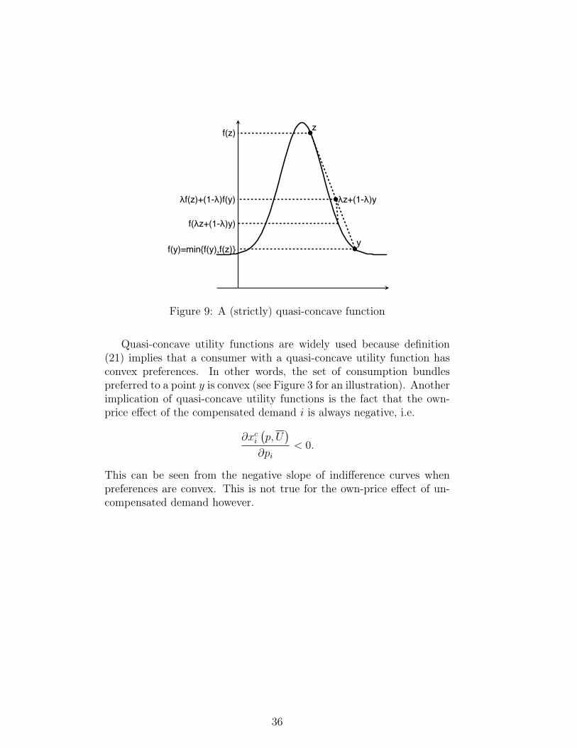
The function in Figure 9 is also strictly quasi-concave. Whereas quasi-concave functions can have many global maxima, strictly quasi-concavefunctions have at most one global maximum. An alternative definitionof a strictly quasi-concave function is that the upper contour set of f isconvex, .i.e. for all z ∈ R

UC (z) ={x ∈ RN |f (x) > z

}. (21)

35

z

y

λz+(1-λ)y

f(z)

f(y)=min{f(y),f(z)}

f(λz+(1-λ)y)

λf(z)+(1-λ)f(y)

Figure 9: A (strictly) quasi-concave function

Quasi-concave utility functions are widely used because definition(21) implies that a consumer with a quasi-concave utility function hasconvex preferences. In other words, the set of consumption bundlespreferred to a point y is convex (see Figure 3 for an illustration). Anotherimplication of quasi-concave utility functions is the fact that the own-price effect of the compensated demand i is always negative, i.e.

∂xci(p, U

)∂pi

< 0.

This can be seen from the negative slope of indifference curves whenpreferences are convex. This is not true for the own-price effect of un-compensated demand however.

36

6 Competitive Equilibrium

So far we have been concerned with a single agent decision problem.Using the tools developed, we can now consider the more interestingsituation where many agents are interacting. One way of modelling theinteraction between many agents is Competitive Equilibrium, or GeneralEquilibrium. In a competitive equilibrium framework the agents are“endowed” with some vector of commodities, and then proceed to tradeat some prices. These prices must be such that the amount offered fortrade (the sum of the agents’ endowments) equals the amount demanded.This trading results in a new allocation, where all mutually beneficialtrades have been exhausted.

We now consider the example of an economy with two agents andtwo goods. The framework is far more general and can be extendedwithout complications to any arbitrary number of agents and goods,but we consider only this case to simplify notation. We assume thatthere are two people in the economy, Robinson and Friday. Since theylive on an island they can only trade with each other. The budget setis simply p1x1 + p2x2 ≤ M as usual. However, the amount of moneyan individual has is simply the value of their endowment. If the initialendowment of good 1 and 2 respectively is e = (e1, e2) then the budgetset is simply

p1x1 + p2x2 ≤ p1e1 + p2e2. (22)Suppose there are two goods, bananas and coconuts, then we can writethe endowments for Robinson and Friday as eR = (eRB, e

RC) and eF =

(eFB, eFC) as the endowments of bananas and coconuts respectively.

Each agent maximizes his utility subject to the budget constraint(22). The problem for Robinson is to solve

maxxR

B ,xRC

uR(xRB, x

RC

)s.t. pBx

RB + pCx

RC ≤ pBe

RB + pCe

RC (23)

and similarly Friday’s problem is to solve

maxxF

B ,xFC

uF(xFB, x

FC

)s.t. pBx

FB + pCx

FC ≤ pBe

FB + pCe

FC (24)

We can then define a competitive equilibrium. This definition can,of course, be extended to more goods, and more agents.

Definition 6.1. A Competitive Equilibrium is a set of prices p = (pB, pC)and a set of consumption choices xR =

(xRB, x

RC

)and xF =

(xFB, x

FC

)such

that at these prices xR solves the utility maximization problem in (23)and xF solves (24), and markets clear so that

xRB + xFB = eRB + eFBxRC + xFC = eRC + eFC

37

So competitive equilibrium consists of an individual problem and asocial problem: agent optimization and market clearing. Basically, thisdefinition means that in a competitive equilibrium all agents take theprices as given, and choose the optimal bundle at these prices. Theprices must be set so the aggregate demand for each good, (the sum ofhow much each agent demands) is equal to the aggregate supply (thesum of all agents’ endowments). We can denote the total endowment ofeach good by eB = eRB + eFB and eC = eRC + eFC .

Here we state two important theorems that we will consider in moredetail later on.

Theorem 6.2. (First Welfare Theorem) Every competitive equilibriumis Pareto efficient.

Theorem 6.3. (Second Welfare Theorem) Every Pareto efficient allo-cation can be decentralized as a competitive equilibrium. That is, everyPareto efficient allocation is the equilibrium for some endowments.

We now consider a simple example, where Friday is endowed withthe only (perfectly divisible) banana and Robinson is endowed with theonly coconut. That is eF = (1, 0) and eR = (0, 1). To keep things simplesuppose that both agents have the same utility function

u(xB, xC) = α√xB +

√xC

and we consider the case where α > 1, so there is a preference for bananasover coconuts that both agents share. We can determine the indifferencecurves for both Robinson and Friday that correspond to the same utilitylevel that the initial endowments provide. The indifference curves aregiven by

uF(eFB,x

FC

)=α√eFB +

√eFC = α = uF (1, 0)

uR(eRB,e

RC

)=α√eRB +

√eRC = 1 = uR(0, 1)

All the allocations between these two indifference curves are Pareto su-perior to the initial endowment.

This is depicted in the Edgeworth box in Figure 10. Note that wehave a total of four axes in the Edgeworth box. The origin for Fridayis in the south-west corner and the amount of bananas he consumes ismeasured along the lower horizontal axis whereas his amount of coconutsis measured along the left vertical axis. For Robinson, the origin isin the north-east corner, the upper horizontal axis depicts Robinson’s

38

F's bananas

F's

coco

nuts

R's bananas

R's

coco

nuts

F's endowment = R's endowment

R's origin

F's origin

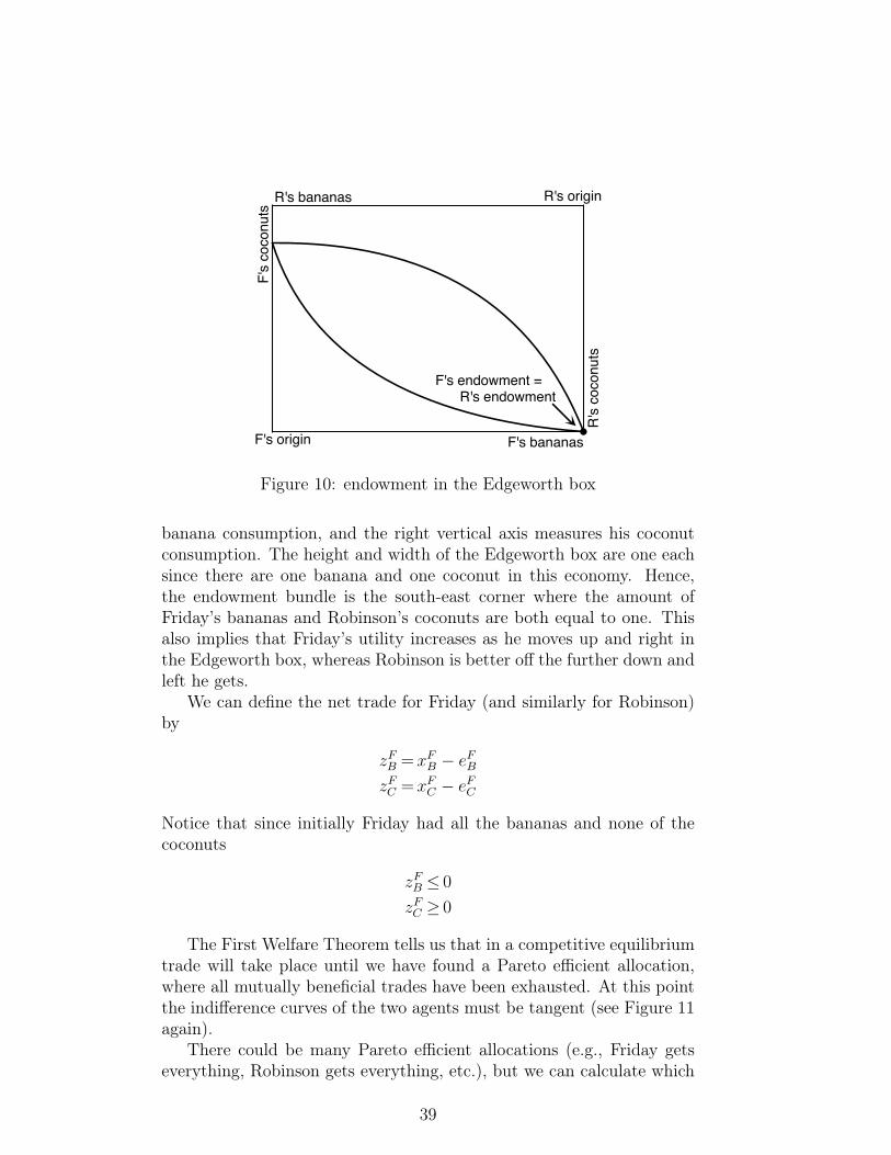
Figure 10: endowment in the Edgeworth box

banana consumption, and the right vertical axis measures his coconutconsumption. The height and width of the Edgeworth box are one eachsince there are one banana and one coconut in this economy. Hence,the endowment bundle is the south-east corner where the amount ofFriday’s bananas and Robinson’s coconuts are both equal to one. Thisalso implies that Friday’s utility increases as he moves up and right inthe Edgeworth box, whereas Robinson is better off the further down andleft he gets.

We can define the net trade for Friday (and similarly for Robinson)by

zFB =xFB − eFBzFC =xFC − eFC

Notice that since initially Friday had all the bananas and none of thecoconuts

zFB ≤ 0

zFC ≥ 0

The First Welfare Theorem tells us that in a competitive equilibriumtrade will take place until we have found a Pareto efficient allocation,where all mutually beneficial trades have been exhausted. At this pointthe indifference curves of the two agents must be tangent (see Figure 11again).

There could be many Pareto efficient allocations (e.g., Friday getseverything, Robinson gets everything, etc.), but we can calculate which

39

F's bananas

F's

coco

nuts

R's bananas

R's

coco

nuts

Pareto efficient allocation

Figure 11: tangent indifference curves in the Edgeworth box

allocations are Pareto optimal. If the indifference curves at an allocationare tangent then the marginal rates of substitution must be equated. Inthis case, the resulting condition is

∂uF

∂xFB

∂uF

∂xFC

=

α

2√xF

B

1

2√xF

C

=

α

2√xR

B

1

2√xR

C

=

∂uR

∂xRB

∂uR

∂xRC

which simplifies to √xFC√xFB

=

√xRC√xRB

and, of course, since there is a total of one unit of each commodity, formarket clearing we must have

xRC = 1− xFCxRB = 1− xFB

so √xFC√xFB

=

√1− xFC√1− xFB

and squaring both sidesxFCxFB

=1− xFC1− xFB

which implies thatxFC − xFCxFB = xFB − xFCxB

40

and so

xFC =xFBxRC =xRB.

So in this example, the Pareto efficient allocations are precisely the 45degree line in the Edgeworth box (see Figure 11).

What are the conditions necessary for an equilibrium? First we needthe conditions for Friday to be optimizing. We can write Robinson’s andFriday’s optimization problems as the corresponding Lagrangian, wherewe generalize the endowments to any eR = (eRB, e

RC) and eF = (eFB, e

FC):

L(xFB, x

FC , λ

F)

= α√xFB +

√xFC + λ

(pBe

FB + eFC − pBxFB − xFC

), (25)

where we normalize pC = 1 without loss of generality. A similar La-grangian can be set up for Robinson’s optimization problem. The first-order conditions for (25) are

∂L∂xFB

=α

2√xFB− λFpB = 0 (26)

∂L∂xFC

=1

2√xFC− λF = 0 (27)

∂L∂λF

= pBeFB + eFC − pBxFB − xFC = 0. (28)

Solving as usual by taking the ratio of equations (26) and (27) we getthe following expression for the relative (to coconuts) price of bananas

pB = α

√xFC√xFB

so that we can solve for xFC as a function of xFB

xFC =(pBα

)2

xFB.

Plugging this into the budget constraint from equation (28) we get

pBxFB +

(pBα

)2

xFB = pBeFB + eFC .

Then we can solve for Friday’s demand for bananas

xFB =pBe

FB + eFC

pB +(pB

α

)2

41

and for coconuts

xFC =(pBα

)2 pBeFB + eFC

pB +(pB

α

)2 .

The same applies to Robinson’s demand functions, of course.Now we have to solve for the equilibrium price pB. To do that we

use the market clearing condition for bananas, which says that demandhas to equal supply (endowment):

xFB + xRB = eFB + eRB.

Inserting the demand functions yields

pBeFB + eFC

pB +(pB

α

)2 +pBe

RB + eRC

pB +(pB

α

)2 = eFB + eRB = eB,

where eB is the social endowment of bananas and we define eC = eFC+eRC .We solve this equation to get the equilibrium price of bananas in theeconomy:

p∗B = α

√eCeB.

So we have solved for the equilibrium price in terms of the primitivesof the economy. This price makes sense intuitively. It reflects relativescarcity in the economy (when there are relatively more bananas thancoconuts, bananas are cheaper) and preferences (when consumers valuebananas more, i.e., when α is larger, they cost more). We can thenplug this price back into the previously found equations both for agents’consumption and have an expression for consumption in terms of theprimitives.

We will conclude this section on competitive equilibrium by reiterat-ing and proving the most famous result in economics, the First WelfareTheorem.

Theorem 6.4. (First Welfare Theorem) Every Competitive Equilibriumallocation x∗ is Pareto Efficient.

Proof. Suppose not. Then there exists another allocation y, which isfeasible, such that

for all n: un(y) ≥ un(x∗)

for some n: un(y) > un(x∗).

42

If un(y) ≥ un(x∗), then the budget constraint (and monotone prefer-ences) implies that

I∑i=1

piyni ≥

I∑i=1

pix∗ni (29)

and for some nI∑i=1

piyni >

I∑i=1

pix∗ni . (30)

Equations (29) and (30) imply that

N∑n=1

I∑i=1

piyni >

N∑n=1

I∑i=1

pix∗ni =

I∑i=1

piei,

where the left-most term is the aggregate expenditure and the right-mostterm the social endowment. This is a contradiction because feasibilityof y means that

N∑n=1

yni ≤N∑n=1

eni = ei

for any n and hence

N∑n=1

I∑i=1

piyni ≤

I∑i=1

piei.

43

7 Producer Theory

We can use tools similar to those we used in the consumer theory sectionof the class to study firm behaviour. In that section we assumed thatindividuals maximize utility subject to some budget constraint. In thissection we assume that firms will attempt to maximize their profits givena demand schedule and production technology.

Firms use inputs or commodities x1, . . . , xI to produce an output y.The amount of output produced is related to the inputs by the produc-tion function y = f(x1, . . . , xI), which is formally defined as follows:

Definition 7.1. A production function is a mapping f : RI+ −→ R+.

The prices of the inputs/commodities are p1, . . . , pI and the outputprice is py. The firm takes prices as given and independent of its deci-sions.

Firms maximize their profits by choosing the optimal amount andcombination of inputs.

maxx1,...,xI

pyf(x1, . . . , xI)−I∑i=1

pixi. (31)

Another way to describe firms’ decision making is by minimizing thecost necessary to produce an output quantity y.

minx1,...,xI

I∑i=1

pixi s.t. f(x1, . . . , xI) ≥ y.

The minimized cost of production, C (y), is called the cost function.We make the following assumption for the production function: pos-

itive marginal product∂f

∂xi≥ 0

and declining marginal product

∂2f

∂x2i

≤ 0.

The optimality conditions for the profit maximization problem (31)and the FOCs for all i

py∂f

∂xi− pi = 0.

44

In other words, optimal production requires equality between marginalbenefits and marginal cost of production. The solution to the profitmaximization problem then is

x∗i (p1, . . . , pI , py), i = 1, . . . , I

y∗(p1, . . . , pI , py),

i.e., optimal demand for inputs and optimal output/supply.The solution of the cost minimization problem (), on the other hand

isx∗i (p1, . . . , pI , y) , i = 1, . . . , I,

where y is the firm’s production target.

Example 7.2. One commonly used production function is the Cobb-Douglas production function where

f(K,L) = KαL1−α

The interpretation is the same as before with α reflecting the relativeimportance of capital in production. The marginal product of capital is∂f∂K

and the marginal product of labor is ∂f∂L

.

In general, we can change the scale of a firm by multiplying bothinputs by a common factor: f(tK, tL) and compare the new output totf(K,L). The firm is said to have constant returns to scale if

tf(K,L) = f(tK, tL),

it has decreasing returns to scale if

tf(K,L) > f(tK, tL),

and increasing returns to scale if

tf(K,L) < f(tK, tL).

Example 7.3. The Cobb-Douglas function in our example has constantreturns to scale since

f(tK, tL) = (tK)α(tL)1−α = tKαL1−α = tf(K,L).

Returns to scale have an impact on market structure. With decreas-ing returns to scale we expect to find many small firms. With increasingreturns to scale, on the other hand, there will be few (or only a single)large firms. No clear prediction can be made in the case of constantreturns to scale. Since increasing returns to scale limit the number offirms in the market, the assumption that firms are price takers onlymakes sense with decreasing or constant returns to scale.

45

8 Decisions under Uncertainty

So far, we have assumed that decision makers have all the needed infor-mation. This is not the case in real life. In many situations, individualsor firms make decisions before knowing what the consequences will be.For example, in financial markets investors buy stocks without knowingfuture returns. Insurance contracts exist because there is uncertainty. Ifindividuals were not uncertain about the possibility of having an acci-dent in the future, there would be no need for car insurance.

8.1 LotteriesTo conceptualize uncertainty, we define the notion of a lottery as follows:

L = {c1, . . . , cN ; p1, . . . , pN} ,

where cn ∈ R is a money award (positive or negative) that will be paidout if the state of the world is n and pn ∈ [0, 1] is the probability thatstate n occurs. For example, a state of the world could be the occurrenceof an accident. Then pn measures the probability that an accident occursand cn is the loss associated with the accident.

Lotteries are nothing else than random variables, which means thatwe can evaluate them using tools from statistics. The expected value ofa lottery (its mean) is defined as

E[L] =N∑n=1

pncn.

For a valid random variables we need the probabilities to be non-negativeand to sum up to one: pn ≥ 0 and

∑Nn=1 pn = 1. Moreover, the c1, . . . , cN

have to be mutually exclusive. A safe lottery or deterministic out-come can be represented by a degenerate probability distribution, forexample (p1, . . . , pN) = (1, 0, . . . , 0). In this case, state n = 1 occurswith certainty. Another way to represent a safe outcome is by havingc1 = · · · = cN ; i.e., all awards are the same. The risk of a lottery can berepresented by its variance, which is defined as

var(L) =N∑n=1

(cn − E[L])2 pn.

Example 8.1. An famous lottery is the following one, also known asthe St. Petersburg paradox. A fair coin is tossed until head comes upfor the first time. Then the reward paid out is equal to 2n, where n is

46

the number of coin tosses that were necessary for head to come up once.This lottery is described formally as

LSP =

{2, 4, 8, . . . , 2n, . . . ;

1

2,1

4,1

8, . . . ,

1

2n, . . .

}.

Its expected value is

E [LSP ] =∞∑n=1

pncn =∞∑n=1

1

2n2n =

∞∑n=1

1 =∞.

Hence the expected payoff from this lottery is infinitely large and anindividual offered this lottery should be willing to pay an infinitely largeamount for the right to play this lottery. This is not what people do,however, hence the paradox.

8.2 Expected UtilityAgents usually do not just consider the mean of lotteries, but also theirrisk. This leads to concave utility functions.

Definition 8.2. A utility function u : R+ −→ R+ is concave if for x, yand all λ ∈ [0, 1]

λu(x) + (1− λ)u(y) ≤ u (λx+ (1− λ)y) ,

where the LHS is the expected values of utility and the RHS is utilityfrom the expected payoff.

In other words, an agent with a concave utility function prefers theexpected value of the lottery to the lottery itself. Figure 12 illustratesthis. We call agents with concave utility function risk avers.

Definition 8.3. The expected utility of a decision maker with utilityfunction u : R+ −→ R+ for a lottery L = {c1, . . . , cN ; p1, . . . , pN} isdefined by

U(L) =N∑n=1

pnu (cn) .

Note the difference between the upper-case U in U(L) and the lower-case u in u (cn); they are two different functions.

Definition 8.4. A decision maker is called risk averse if the utilityfunction u : R+ −→ R+is concave and she is called risk loving or a riskseeker if u is convex.

47

x λx+(1-λ)y y

u(x)

u(y)

u(λx+(1-λ)y)

λu(x)+(1-λ)u(y)

Figure 12: A concave utility function

8.3 InsuranceAn important application for uncertainty is insurance contracts. Con-sider a world with two states, one where an accident occurs and onewithout an accident. In both states, the agent’s wealth is w. An ac-cident occurs with probability π ∈ (0, 1) and the damage in case of anaccident is D > 0. The agent can buy insurance of $1 at the price ofq. The amount of insurance bought is α. Then we can summarize thepayoffs as follows:

state of the world payoff

no accident w − αqaccident w −D − αq + q

The goal is to determine the optimal level of insurance, α∗. To dothat, we maximize the agent’s expected utility over α:

maxα{πu (w −D − αq + q) + (1− π)u (w − αq)} .

The FOC is

πu′ (w −D − αq + q) (1− q)− (1− π)u′ (w − αq) q = 0. (32)

In words, the marginal utility in the bad state (benefit of insurance) hasto equal the marginal utility in the good state (cost of insurance).

Now, we assume that the insurance company sells “fair insurance,”which means that it sets an actuarially fair price so that it has an ex-pected payoff of zero.6 Hence the expected payment if an accident occurs,

6This is obviously not a very realistic assumption.

48

π, has to equal the premium q. The FOC (32) at q = π becomes

πu′ (w −D − αq + q) (1− π)− (1− π)u′ (w − αq) π = 0⇐⇒u′ (w −D − αq + q) = u′ (w − αq) ,

which implies the solution α∗ = D, assuming a strictly concave utilityfunction with u′′(w) < 0. Hence, in order to equalize marginal utility inboth states, the wealth in both states is the same. This is also knownas full insurance.

49

9 Pricing Power

So far, we have considered market environments where single agent can-not control prices. Instead, each agent was infinitesimally small andfirms acted as price takers. This was the case in competitive equilib-rium. There are many markets with few (oligopoly) or a single firms,(monopoly) however. In that case firms can control prices to some ex-tent. Moreover, when there are a few firms in a market, firms makeinteractive decisions. In other words, they take their competitors’ ac-tions into account. In Section 10, we will use game theory to analysethis type of market structure. First, we cover monopolies, i.e., marketswith a single producer.

9.1 MonopolyIf a firm produces a non-negligible amount of the overall market then theprice at which the good sells will depend on the quantity sold. Examplesfor firms that control the overall market include the East India TradingCompany, Microsoft (software in general because of network external-ities and increasing returns to scale), telecommunications and utilities(natural monopolies), Standard Oil, and De Beers.

For any given price there will be some quantity demanded by con-sumers, and this is known as the demand curve x : R+ −→ R+ or simplyx(p). We assume that consumers demand less as the price increases: thedemand function is downward sloping or x′(p) < 0. We can invert thisrelationship to get the inverse demand function p(x) which reveals theprice that will prevail in the market if the output is x.

If the firm is a monopolist that takes the demand data p(x) as giventhen its goal is to maximize

π(x) = p(x)x− c(x) (33)

by choosing the optimal production level. For the cost function we as-sume c′(x) > 0 and c′′(x) ≥ 0, i.e., we have positive and weakly increas-ing marginal costs. For example, c(x) = cx satisfies these assumptions(a Cobb-Douglas production function provides this for example). Themonopolist maximizes its profit function (33) over x, which leads to thefollowing FOC:

p(x) + xp′(x)− c′(x) = 0. (34)

Here, in addition to the familiar p(x), which is the marginal returnfrom the marginal consumer, the monopolist also has to take the xp′(x)into account, because a change in quantity also affects the inframarginalconsumers. For example, when it increases the quantity supplies, themonopolist gets positive revenue from the marginal consumer, but the

50

inframarginal consumers pay less due to the downward sloping demandfunction. At the optimum, the monopolist equates marginal revenue andmarginal cost.

Example 9.1. A simple example used frequently is p(q) = a− bq, andwe will also assume that a > c since otherwise the cost of producing ishigher than any consumer’s valuation so it will never be profitable forthe firm to produce and the market will cease to exist. Then the firmwant to maximize the objective

π(x) = (a− bx− c)x.

The efficient quantity is produced when p(x) = a− bx = c because thena consumer buys an object if and only if they value it more than thecost of producing, resulting in the highest possible total surplus. So theefficient quantity is

x∗ =a− cb

.

The monopolist’s maximization problem, however, has FOC

a− 2bx− c = 0

where a− 2bx is the marginal revenue and c is the marginal cost. So thequantity set by the monopolist is

xM =a− c

2b< x∗.

The price with a monopoly can easily be found since

pM = a− bxM

= a− a− c2

=a+ c

2>c.

Figure 13 illustrates this.

A monopoly has different welfare implications than perfect compe-tition. In Figure 13, consumers in a monopoly lose the areas A andB compared to perfect competition. The monopolist loses area C andwins area A. Hence, there are distributional implications (consumers loseand the producer gains) as well as efficiency implications (overall welfaredecreases).

51

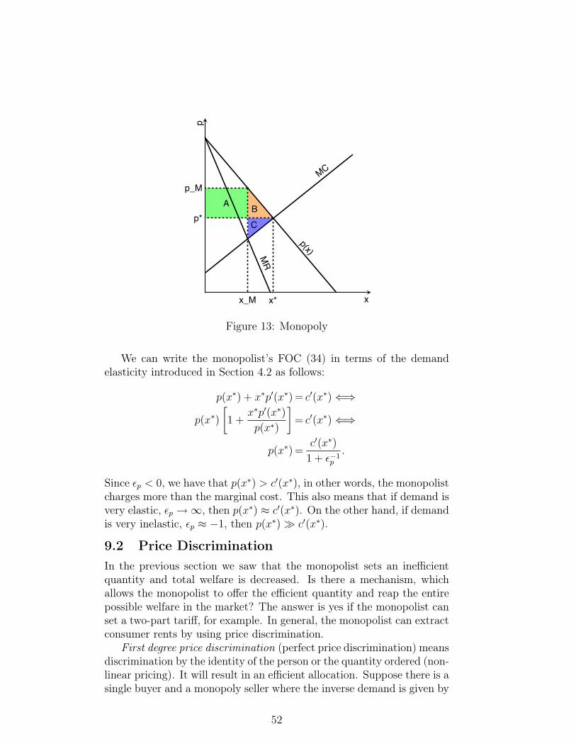
x

p

x_M

p_M

x*

p*A B

C

MC

p(x)MR

Figure 13: Monopoly

We can write the monopolist’s FOC (34) in terms of the demandelasticity introduced in Section 4.2 as follows:

p(x∗) + x∗p′(x∗) = c′(x∗)⇐⇒

p(x∗)

[1 +

x∗p′(x∗)

p(x∗)

]= c′(x∗)⇐⇒

p(x∗) =c′(x∗)

1 + ε−1p

.

Since εp < 0, we have that p(x∗) > c′(x∗), in other words, the monopolistcharges more than the marginal cost. This also means that if demand isvery elastic, εp →∞, then p(x∗) ≈ c′(x∗). On the other hand, if demandis very inelastic, εp ≈ −1, then p(x∗)� c′(x∗).

9.2 Price DiscriminationIn the previous section we saw that the monopolist sets an inefficientquantity and total welfare is decreased. Is there a mechanism, whichallows the monopolist to offer the efficient quantity and reap the entirepossible welfare in the market? The answer is yes if the monopolist canset a two-part tariff, for example. In general, the monopolist can extractconsumer rents by using price discrimination.

First degree price discrimination (perfect price discrimination) meansdiscrimination by the identity of the person or the quantity ordered (non-linear pricing). It will result in an efficient allocation. Suppose there is asingle buyer and a monopoly seller where the inverse demand is given by

52

p = a− bx. If the monopolist were to set a single price it would set themonopoly price. As we saw in the previous section, however, this doesnot maximize the joint surplus, so the monopolist can do better. Supposeinstead that the monopolist charges a fixed fee F that the consumer hasto pay to be allowed to buy any positive amount at all, and then sells thegood at a price p, and suppose the monopolist sets the price p = c. Thefixed fee will not affect the quantity that a participating consumer willchoose, so if the consumer participates then they will choose quantityequal to x∗. The firm can then set the entry fee to extract all theconsumer surplus and the consumer will still be willing to participate.This maximizes the joint surplus, and gives the entire surplus to thefirm, so the firm is doing as well as it could under any other mechanism.Specifically, using the functional form from Example 9.1 the firm sets

F =(a− c)x∗

2=

(a− c)2

2b

In integral notation this is

F =

x∗∫0

(p(x)− c)dx.

This pricing mechanism is called a two-part tariff, and was famously usedat Disneyland (entry fee followed by a fee per ride), greatly increasingrevenues.

Now, let’s assume that there are two different classes of consumers,type A with utility function u(x) and type B with βu(x), β > 1, so thatthe second class of consumers has a higher valuation of the good. If themonopolist structures a two-part tariff (F, p = c) to extract all surplusfrom type B consumers, type A consumers would not pay the fixed feeF since they could not recover the utility lost from using the service.On the other hand, if the firm offers two two-part tariffs (FA, p = c)and (FB, p = c) with FA < FB, all consumers would pick the cheapercontract (FA, p = c). A solution to this problem would be to offer thecontracts (FA, pA > c) and (FB, p = c). Type A consumers pick the firstcontract and consume less of the good and type B consumers pick thesecond contract, which allows them to consume the efficient quantity.This is an example for second degree price discrimination, which meansthat the firm varies the price by quantity or quality only. It offers amenu of choices and lets the consumers self-select into their preferredcontract.

In addition, there is third degree price discrimination, in which thefirm varies the price by market or identity of the consumers. For ex-ample, Disneyland can charge different prices in different parks. Let’s

53

assume there are two markets, i = 1, 2. The firm is a monopolist in bothmarkets and its profit maximization problem is

maxx1,x2

x1p1(x1) + x2p2(x2)− c(x1 + x2).

The FOC for each market is

pi(xi) + xip′i(xi) = c′(x1 + x2),

which leads to optimal solution

pi(x∗i ) =

c′(x∗1 + x∗2)

1 + 1εip

for i = 1, 2.

Hence, the solution depends on the demand elasticity in market i. Theprice will be different as long as the structure of demand differs.

54

10 Oligopoly

Oligopoly refers to environments where there are few large firms. Thesefirms are large enough that their quantity influences the price and so im-pacts their rivals. Consequently each firm must condition its behaviouron the behaviour of the other firms. This strategic interaction is mod-elled with game theory.

10.1 DuopolyProbably the most important model of oligopoly is the Cournot modelof quantity competition. We will first consider the duopoly case, wherethere are only two firms. Suppose the inverse demand function is givenby p(q) = a− bq, and the cost of producing is constant and the same forboth firms ci(q) = cq. The quantity produced in the market is the sumof what both firms produce q = q1 + q2. The profits for each firm is thena function of the market price and their own quantity,

πi(qi, qj) = qi (p (qi + qj)− c) .

The strategic variable that the firm is choosing is the quantity to produceqi.

Suppose that the firms’ objective was to maximize their joint profit

π1(q1, q2) + π2(q1, q2) = (q1 + q2) (p (q1 + q2)− c)

then we know from before that this is maximized when q1 + q2 = qM .We could refer to this as the collusive outcome. One way the two firmscould split production would be q1 = q2 = qM

2.

If the firms could write binding contracts then they could agree onthis outcome. However, that is typically not possible (such an agreementwould be price fixing), so we would not expect this outcome to occurunless it is stable/self-enforcing. If either firm could increase its profitsby setting another quantity, then they would have an incentive to deviatefrom this outcome. We will see below that both firms would in fact havean incentive to deviate and increase their output.

Suppose now that firm i is trying to choose qi to maximize its ownprofits, taking the other firm’s output as given. Then firm i’s optimiza-tion problem is

maxqi

πi(qi, qj) = qi (a− b (qi + qj)− c) ,

which has the associated FOC

∂πi(qi, qj)

∂qi= a− b (2qi + qj)− c = 0.

55

q1

q2

1

0.5

0.5 1

q1(q2)

q2(q1)

Nash Equilibrium

Figure 14: Cournot equilibrium

Then the optimal level q∗i given any level of qj is

q∗i (qj) =a− bqj − c

2b.

This is firm i’s best response to whatever firm j plays. In the specialcase when qj = 0 firm i is a monopolist, and the observed quantityqi corresponds to the monopoly case. In general, when the rival hasproduced qj we can treat the firm as a monopolist facing a “residualdemand curve” with intercept of a − bqj. We can write firm i’s bestresponse function as

q∗i (qj) =a− c

2b− 1

2qj.

Hence,dqidqj

= −1

2.

This has two important implications. First, the quantity player ichooses is decreasing in its rival’s quantity. This means that quantitiesare strategic substitutes. Second, if player j increases their quantityplayer i decreases their quantity by less than player j increased theirquantity (player i decreases his quantity by exactly 1

2for every unit

player j’s quantity is increased). So we would expect that the output ina duopoly would be higher than in a monopoly.

We can depict the best response function graphically. Setting a =b = 1 and 0, Figure 14 shows the best response functions. Here, the bestresponse functions are q∗i (qj) =

1−qj2

.

56

We are at a “stable” outcome if both firms are producing a bestresponse to their rivals’ production. We refer to such an outcome as anequilibrium. That is, when

qi =a− bqj − c

2b

qj =a− bqi − c

2b.

Since the best responses are symmetric we will have qi = qj and so wecan calculate the equilibrium quantities from the equation

qi =a− bqi − c

2b

and soqi = qj =

a− c3b

and henceq = qi + qj =

2(a− c)3b

>a− c

2b= qM .

There is a higher output (and hence lower price) in a duopoly then amonopoly.

More generally, both firms are playing a best response to their rival’saction because for all i

πi(q∗i , q∗j ) ≥ πi(qi, q

∗j ) for all qi

That is, the profits from the quantity are (weakly) higher then the profitsfrom any other output. This motivates the following definition for anequilibrium in a strategic setting.

Definition 10.1. A Nash Equilibrium in the duopoly game is a pair(q∗i , q

∗j ) such that for all i

πi(q∗i , q∗j ) ≥ πi(qi, q

∗j ) for all qi.

This definition implicitly assumes that agents hold (correct) expec-tations or beliefs about the other agents’ strategies.

A Nash Equilibrium is ultimately a stability property. There is noprofitable deviation for any of the players. In order to be at equilibriumwe must have that

qi = q∗i (qj)

qj = q∗j (qi)

57

and so we must have that

qi = q∗i (q∗j (qi))

so equilibrium corresponds to a fixed-point of the mapping q∗1(q∗2(·)). Thisidea can also be illustrated graphically. In Figure 14, firm 1 initially setsq1 = 1

2, which is not the equilibrium quantity. Firm 2 then optimally

picks q2 = q∗2(

12

)= 1

4according to its best response function. Firm 1,

in turn, chooses a new quantity according to its best response function:q1 = q∗1

(14

)= 3

8. This process goes on and ultimately converges to

q1 = q2 = 13.

10.2 General CournotNow, we consider the case with I competitors. The inverse demandfunction (setting a = b = 1) is

p(q) = 1−I∑i=1

qi

and firm i’s profit function is

π(qi, q−i) =

(1−

I∑i=1

qi − c

)qi, (35)

where the vector q−i is defined as q−i = (q1, . . . , qi−1, qi+1, . . . , qI), i.e.,all quantities excluding qi.

Again, we can define an equilibrium in this market as follows:

Definition 10.2. A Nash Equilibrium in the oligopoly game is a vectorq∗ = (q∗1, . . . , q

∗I ) such that for all i

πi(q∗i , q∗−i) ≥ πi(qi, q

∗−i) for all qi.

We simply replaced the quantity qj by the vector q−i.

Definition 10.3. A Nash equilibrium is called symmetric if q∗i = q∗j forall i and j.

The FOC for maximizing the profit function (35) is

1−∑j 6=i

qj − 2qi − c = 0

and the best response function for all i is

qi =1−

∑j 6=i qj − c2

. (36)

58

Here, only the aggregate supply of firm i’s competitors matters, but notthe specific amount single firms supply. It would be difficult to solve forI separate values of qi, but due to symmetry of the profit function weget that q∗i = q∗j for all i and j so that equation (36) simplifies to

q∗i =1− (I − 1)q∗i − c

2,

which leads to the solution

q∗i =1− cI + 1

.

As I increases (more firms), the market becomes more competitive.Market supply is equal to

I∑i=1

q∗i = Iq∗i =I

I + 1(1− c).

As the number of firms becomes larger, I −→∞, q∗i −→ 0 and

I∑i=1

q∗i −→ 1− c,

which is the supply in a competitive market. As each player plays a lessimportant strategical role in the market, the oligopoly outcome convergesto the competitive market outcome.

Note that we used symmetry in deriving the market outcome fromthe firms’ best response function. We cannot invoke symmetry whenderiving the FOC. One might think that instead of writing the profitfunction as (35) one could simplify it to

π(qi, q−i) = (1− Iqi − c) qi.

This is wrong, however, because it implies that firm i controls the entiremarket supply (acts as a monopolist). Instead, in an oligopoly market,firm i takes the firms’ output as given.

10.3 Stackelberg GameIn the Counot game in Section 10.1 two firms choose their quantitiessimultaneously. In many markets, however, one firm (the leader or firstmover) might make a decision before the other (the follower or secondmover). The most natural interpretation is that the leader is the incum-bent in the market, and the second firm is a new entrant. Then, the first

59

mover can anticipate the second mover’s action and pick its quantitytaking the other firm’s best response into account. This situation differsfrom the Cournot game because the leader can commit to a quantity be-fore the follower makes a decision. Since firm 1 must take into accountthe effect of their quantity on firm 2, we use “backward induction” tosolve this game. We first determine what firm 2 will produce in responseto any quantity from quantity 1 in the first period. The first firm takesfirm 2’s response to its quantity into account when it sets its quantityin the first period.

As before the profit function for firm i = 1, 2 is

πi(qi, qj) = [a− b(qi + qj)− c] qi.

Using backward induction, we first determine firm 2’s (the follower)choice given any quantity supplied by firm 1. In other words, we haveto derive firm 2’s best response as before. The follower’s profit functionis

π2(q1, q2) = [a− b(q1 + q2)− c] q2

and the FOC isdπ2

dq2

= a− bq1 − 2bq2 − c = 0,

which leads to firm 2’s best response

q∗2(q1) =a− c

2b− q1

2.

Again we see that

q′2(q1) = −1

2< 0

which implies that q1 and q2 are strategic substitutes.Now in the first period, the leader knows how their rival will respond

to whatever quantity they produce and will take this into account whensetting quantity. So firm 1 chooses quantity to maximize

π1(q1) =π1 (q1, q∗2(q1))

= [a− b (q1 + q∗2(q1))− c] q1

=

[a− b

(q1 +

a− c2b− q1

2

)− c]q1

=

(a− c

2− b

2q1

)q1,

which has the associated FOC

dπ1

dq1

=a− c

2− bq1 = 0

60

and thenq∗1 =

a− c2b

= qM > qC1 .

The leader chooses the same quantity as a monopolist in this market.In particular, it chooses a larger quantity than each firm in the Cournotgame. The follower acts upon firm 1’s chosen quantity by playing itsbest response:

q∗2 =a− c

2b− q∗1

2=a− c

2b− a− c

4b=a− c

4b< qC2 .

Hence we notice that firm 1 exploits its first mover advantage to producemore than its rival. Notice also that q1 +q2 = 3a

4bwhich is higher then the

total output of the Cournot game. This is because firm 1, anticipatingits affect on its rival, produces more than the Cournot output, and firm2 only cuts back production by 1

2for each addition unit firm 1 produces.

The key here was that firm 1 was able to commit to the high output.If it could go back and adjust its output at the end it would under-mine this commitment and remove the first mover advantage. So therestriction that the firm cannot go back and adjust its output is actuallybeneficial. In the single agent decision problem constraints are neverbeneficial, but in a strategic environment they may be. Firm 2 whichis at a disadvantage could try to threaten to produce more to try toprevent firm 1 from producing so much, but such a claim would not becredible (since if firm 2 does not play a best response it decreases itsown profits). Of course, we have assumed that the follower is motivatedsolely by the desire to maximize its profits in this period (i.e., no fu-ture periods where their behaviour this period can influence the futurepayoff).

10.4 Vertical ContractingIn many markets we can observe more than two kinds of participants.It is common, for example, to have a producer or wholesaler who sellsgoods or services to a retailer or distributor who in turn sells them tothe final consumer. The wholesaler is also known as the upstream firmand the retailer is called the downstream firm. This situation can leadto double marginalization, which means that both the upstream and thedownstream firms act as monopolists thereby adding a margin to theircosts and decreasing the quantity sold. The following simple modelillustrates this.

Suppose the final consumer’s inverse demand function is

p = a− bq.

61

Then the retailer’s profit function is

πR(qR) = (a− bqR − pW )qR,

where pW is the price set by the wholesaler (the unit cost for the retailer)and qR is the quantity set by the retailer. The FOC is

a− 2bqR − pW = 0

which can be solved as

q∗R(pW ) =a− pW

2b. (37)

Hence the price charged by the retailer is

p∗R(pW ) =a+ pW

2> pW

since we assume that a > pW so that at least the first marginal consumerdemands the good. The “pass through rate” is 1

2: for a $1 price increase

by the wholesaler, the retailer increase the final price by $0.50. Sinceprice increases are passed through imperfectly, the upstream firm has alarger incentive to increase pW .

Now we calculate the optimal price pW given the retailer’s optimalsupply function (37). The wholesaler’s profit is

πW (pW ) = pW q∗R(pW ) = pW

a− pW2b

assuming that the wholesaler’s cost of producing the good is 0. TheFOC is

a− 2pW = 0

so that the upstream firm sets the optimal price

p∗W =a

2.

Plugging this into the retailer’s best response functions we get

p∗R(p∗W ) =3a

4

andq∗R(p∗W ) =

a

4b< q∗M =

a

2b.

Hence, the quantity under this market structure is even lower than ina monopoly. In general, deeper distribution makes the outcome lessefficient.

62

One solution to alleviate this inefficiency would be vertical integra-tion: By merging the upstream and downstream firm we could get ridof the retailer. Note that this is different from horizontal integration,which refers to mergers between firms on the same level of the distribu-tional chain. Since vertical integration leads to social surplus due to aless inefficient quantity it is important to distinguish between these twotypes of integration when evaluating a potential merger.

Another solution to avoid double marginalization is a two-part tariff(FW , rW ), where the retailer pays FW to obtain the right to distributethe good (participation fee) and then pays rW for every unit purchasedfrom the wholesaler. An example for this strategy is the market forrental videos. Optimally, the the wholesaler sets r∗W = 0 to induce theretailer to sell as many units as possible (q∗R in equation (37) dependsnegatively on pW ) and then sets F ∗W so that the retailer just participates,but the wholesaler can capture the entire payoff of the downstream firm.In our model,

F ∗W = π∗R =( a

2b

)2

.

The distributional implications of the two-part tariff are as follows: theconsumers’ payoff increases since they get a higher quantity at a lowerprice and the wholesaler’s payoff increases because it extracts all thesurplus from the retailer. In our case, the retailer loses all its surplus,but this is not true in general.

63

11 Game Theory

In the previous section we introduced game theory in the context of firmcompetition. In this section, we will generalize the methods used aboveand introduce some specific language. The specification of (static) gameconsists of three elements:

1. The players, indexed by i = 1, . . . , I. In the duopoly games, forexample, the players were the two firms.

2. The strategies available: each player chooses strategy si from theavailable strategy set Si.We can write s−i = (s1, . . . , si−1, si+1, . . . , sI)to represent the strategies of the other I−1 players. Then, a strat-egy profile of all players is defined by s = (s1, . . . , sI) = (si, s−i).In the Cournot game, the player’s strategies were the quantitieschose, hence Si = R+.

3. The payoffs for each player as a function of the strategies of theplayers. We use game theory to analyze situations where there isstrategic interaction so the payoff function will typically depend onthe strategies of other players as well. We write the payoff functionfor player i as ui(si, s−i). The payoff function is the mapping

ui : S1 × · · · × SI −→ R.

The definition we have given above for a Nash Equilibrium in the oligopolygame extends to games in general.

Definition 11.1. A strategy profile s∗ = (s∗1, . . . , s∗I) is a Nash Equilib-

rium if, for all i

ui(s∗i , s

∗−i)≥ ui

(si, s

∗−i)for all si ∈ Si.

We refer to strategy s∗i as a best response to s∗−i.

11.1 Pure StrategiesWe can represent games (at least those with a finite choice set) in normalform. A normal form game consists of the matrix of payoffs for eachplayer from each possible strategy. If there are two players, 1 and 2,then the normal form game consists of a matrix where the (i, j)th entryconsists of the tuple (player 1’s payoff, player2’s payoff) when player 1plays their ith strategy and player 2 plays their jth strategy. We willnow consider the most famous examples of games.

64

Example 11.2. (Prisoner’s Dilemma) Suppose two suspects, Bob andRob are arrested for a crime and questioned separately. The police canprove the committed a minor crime, and suspect they have committeda more serious crime but can’t prove it. The police offer each suspectthat they will let them off for the minor crime if they confess and testifyagainst their partner for the more serious crime. Of course, if the othercriminal also confesses the police won’t need his testimony but will givehim a slightly reduced sentence for cooperating. Each player then hastwo possible strategies: Stay Quiet (Q) or Confess (C) and they decidesimultaneously. We can represent the game with the following payoffmatrix:

RobQ C

Bob Q 3, 3 −1, 4C 4, −1 0, 0

Each entry represents (Bob, Rob)’s payoff from each of the two strate-gies. For example, if Rob stays quiet while Bob confesses Bob’s payoffis 4 and Rob’s is −1. Notice that both players have what is known asa dominant strategy; they should confess regardless of what the otherplayer has done. If we consider Bob, if Rob is Quiet then confessinggives payoff 4 > 3, the payoff from staying quiet. If Rob confesses, thenBob should confess since 0 > −1. The analysis is the same for Rob. Sothe only stable outcome is for both players to confess. So the only NashEquilibrium is (Confess, Confess). Notice that, from the perspective ofthe prisoners this is a bad outcome. In fact it is Pareto dominated byboth players staying quiet, which is not a Nash equilibrium.

The above example has a dominant strategy equilibrium, where bothplayers have a unique dominant strategy.

Definition 11.3. A strategy is si is dominant if

ui(si, s−i) > ui(s′i, s−i) for all s′i ∈ Si, s−i ∈ S−i.

If each player has a dominant strategy, then the only rational thingfor them to do is to play that strategy no matter what the other playersdo. Hence, if a dominant strategy equilibrium exists it is a relativelyuncontroversial prediction of what will happen in the game. However,it is rare that a dominant strategy will exist in most strategic situa-tions. Consequently, the most commonly used solution concept is NashEquilibrium, which does not require dominant strategies.

65

Note the difference between Definitions 11.1 and 11.3: A Nash Equi-librium is only defined for the best response of the other players, s∗−i,whereas dominant strategies have to hold for strategies s−i ∈ S−i. Astrategy profile is a Nash Equilibrium if each player is playing a bestresponse to the other players’ strategies. So a Nash Equilibrium is astable outcome where no player could profitably deviate. Clearly whendominant strategies exist it is a Nash Equilibrium for all players to play adominant strategy. However, as we see from the Prisoner’s Dilemma ex-ample the outcome is not necessarily efficient. The next example showsthat the Nash Equilibrium may not be unique.

Example 11.4. (Coordination Game) We could represent a coordina-tion game where Bob and Ann are two researcher both of whose inputis necessary for a project. They decide simultaneously whether to doresearch (R) or not (N).

BobR N

Ann R 3, 3 −1, 0N 0, −1 1, 1

Here (R,R) and (N,N) are both equilibria. Notice that the equilibriain this game are Pareto ranked with both players preferring to coordinateon doing research. Both players not doing research is also an equilibrium,since if both players think the other will play N they will play N as well.

A famous example of a coordination game is from traffic control. Itdoesn’t really matter if everyone drives on the left or right, as long aseveryone drives on the same side.

Example 11.5. Another example of a game is a “beauty contest.” Ev-eryone in the class picks a number on the interval [1, 100]. The goal isto guess as close as possible to 2

3the class average. An equilibrium of

this game is for everyone to guess 1. This is in fact the only equilibrium.Since no one can guess more than 100, 2

3of the mean cannot be higher

than 6623, so all guesses above this are dominated. But since no one will

guess more than 6623the mean cannot be higher than 2

3(662

3) = 444

9,

so no one should guess higher than 4449. Repeating this n times no one

should guess higher than(

23

)n100 and taking n −→∞ all players should

guess 1. Of course, this isn’t necessarily what will happen in practiceif people solve the game incorrectly or expect others too. Running thisexperiment in class the average guess was approximately 12.

66

11.2 Mixed StrategiesSo far we have considered only pure strategies: strategies where theplayers do not randomize over which action they take. In other words,a pure strategy is a deterministic choice. The following simple exampledemonstrates that a pure strategy Nash Equilibrium may not alwaysexist.

Example 11.6. (Matching Pennies) Consider the following payoff ma-trix:

BobH T

Ann H 1, −1 −1, 1T −1, 1 1, −1

Here Ann wins if both players play the same strategy, and Bob winsif they play different ones. Clearly there cannot be pure strategy equilib-rium, since Bob would have an incentive to deviate whenever they playthe same strategy and Ann would have an incentive to deviate if theyplay the differently. Intuitively, the only equilibrium is to randomizebetween H and T with probability 1

2each.

While the idea of a matching pennies game may seem contrived, it ismerely the simplest example of a general class of zero-sum games, wherethe total payoff of the players is constant regardless of the outcome. Con-sequently gains for one player can only come from losses of the other.For this reason, zero-sum games will rarely have a pure strategy Nashequilibrium. Examples would be chess, or more relevantly, competitionbetween two candidates or political parties. Cold War power politicsbetween the US and USSR was famously (although probably not accu-rately) modelled as a zero-sum game. Most economic situations are notzero-sum since resources can be used inefficiently.

Example 11.7. A slight variation is the game of Rock-Paper-Scissors.

BobR P S

R 0, 0 −1, 1 1, −1Ann P 1, −1 0, 0 −1, 1

S −1, 1 1, −1 0, 0

Definition 11.8. A mixed strategy by player i is a probability distribu-

67

tion σi =(σi (S

1i ) , . . . , σi

(SKi))

such that

σi(ski)≥ 0

K∑k=1

σi(ski)

= 1.

Here we refer to si as an action and to σi as a strategy, which in thiscase is a probability distribution over actions. The action space is Si ={s1i , . . . , s

Ki

}.

Expected utility from playing action si when the other player playsstrategy σj is

ui (si, σj) =K∑k=1

σj(skj)ui(si, s

kj

).

Example 11.9. Consider a coordination game (also knows as “battle ofthe sexes” similar to the one in Example 11.4 but with different payoffs

BobσB 1− σBO C

Ann σA O 1, 2 0, 01− σA C 0, 0 2, 1

Hence Bob prefers to go to the opera (O) and prefers to go to a cricketmatch (C), but both players would rather go to an event together thanalone. There are two pure strategy Nash Equilibria: (O,O) and (C,C).We cannot make a prediction, which equilibrium the players will pick.Moreover, it could be the case that there is a third Nash Equilibrium,in which the players randomize.

Suppose that Ann plays O with probability σA and C with probabil-ity 1− σA. Then Bob’s expected payoff from playing O is

2σA + 0(1− σA) (38)

and his expected payoff from playing C is

0σA + 1(1− σA). (39)

Bob is only willing to randomize between his two pure strategies if hegets the same expected payoff from both. Otherwise he would play thepure strategy that yields the highest expected payoff for sure. Equating(38) and (39) we get that

σ∗A =1

3.

68

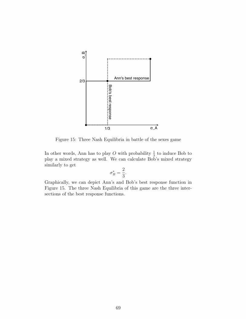
σ_A

σ_B

2/3

1/3

Bob's best response

Ann's best response

Figure 15: Three Nash Equilibria in battle of the sexes game

In other words, Ann has to play O with probability 13to induce Bob to

play a mixed strategy as well. We can calculate Bob’s mixed strategysimilarly to get

σ∗B =2

3.

Graphically, we can depict Ann’s and Bob’s best response function inFigure 15. The three Nash Equilibria of this game are the three inter-sections of the best response functions.

69

12 Asymmetric Information

Asymmetric information simply refers to situations where some of theplayers have relevant information that other players do not. We considertwo types of asymmetric information: adverse selection, also known ashidden information, and moral hazard or hidden action.

A leading example for adverse selection occurs in life or health insur-ance. If an insurance company offers actuarially fair insurance it attractsinsurees with above average risk whereas those with below average riskdecline the insurance. (This assumes that individuals have private infor-mation about their risk.) In other words, individuals select themselvesinto insurance based on their private information. Since only the higherrisks are in the risk pool the insurance company will make a loss. Inconsequence of this adverse selection the insurance market breaks down.Solutions to this problems include denying or mandating insurance andoffering a menu of contracts to let insurees self-select thereby revealingtheir risk type.

Moral hazard is also present in insurance markets when insurees’ ac-tions depend on having insurance. For example, they might exerciseless care when being covered by fire or automobile insurance. This un-dermines the goal of such insurance, which is to provide risk sharing inthe case of property loss. With moral hazard, property loss becomesmore likely because insurees do not install smoke detectors, for example.Possible solutions to this problem are copayments and punishment fornegligence.

12.1 Adverse SelectionThe following model goes back to George Akerlof’s 1970 paper on “Themarket for lemons.” The used car market is a good example for adverseselection because there is variation in product quality and this variationis observed by sellers, but not by buyers.

Suppose there is a potential buyer and a potential seller for a car.Suppose that the quality of the car is denoted by θ ∈ [0, 1]. Buyers andsellers have different valuations/willingness to pay vb and vs, so that thevalue of the car is vbθ to the buyer and vsθ to the seller. Assume thatvb > vs so that the buyer always values the car more highly then theseller. So we know that trade is always efficient. Suppose that boththe buyer and seller know θ, then we have seen in the bilateral tradingsection that trade can occur at any price p ∈ [vsθ, vbθ] and at that pricethe efficient allocation (buyer gets the car) is realized (the buyer has anet payoff of vbθ − p and the seller gets p− vsθ, and the total surplus isvbθ − vsθ).

70

The assumption that the buyer knows the quality of the car maybe reasonable in some situations (new car), but in many situations theseller will be much better informed about the car’s quality. The buyerof a used car can observe the age, mileage, etc. of a car and so havea rough idea as to quality, but the seller has presumably been drivingthe car and will know more about it. In such a situation we couldconsider the quality θ as a random variable, where the buyer knows onlythe distribution but the seller knows the realization. We could considera situation where the buyer knows the car is of a high quality withsome probability, and low quality otherwise, whereas the seller knowswhether the car is high quality. Obviously the car could have a morecomplicated range of potential qualities. If the seller values a high qualitycar more, then their decision to participate in the market potentiallyreveals negative information about the quality, hence the term adverseselection. This is because if the car had higher quality the seller would beless willing to sell it at any given price. How does this type of asymmetricinformation change the outcome?

Suppose instead that the buyer only knows that θ ∼ U [0, 1]. That isthat the quality is uniformly distributed between 0 and 1. The the selleris willing to trade if

p− vsθ ≥ 0 (40)

and the buyer, who does not know θ, but forms its expected value, iswilling to trade if

E[θ]vb − p ≥ 0. (41)

However, the buyer can infer the car’s quality from the price the selleris asking. Using condition (40), the buyer knows that

θ ≤ p

vs

so that condition (41) becomes

E

[θ

∣∣∣∣θ ≤ p

vs

]vb − p =

p

2vsvb − p ≥ 0, (42)

where we use the conditional expectation of a uniform distribution:

E[θ|θ ≤ a] =a

2.

Hence, simplifying condition (42), the buyer is only willing to trade if

vb ≥ 2vs.

71

In other words, the buyer’s valuation has to exceed twice the seller’svaluation for a trade to take place. If

2vs > vb > vs

trade is efficient, but does not take place if there is asymmetric informa-tion.

In order to reduce the amount of private information the seller canoffer a warranty of have a third party certify the car’s quality.

If we instead assumed that neither the buyer or the seller know therealization of θ then the high quality cars would not be taken out ofthe market (sellers cannot condition their actions on information theydo not have) and so we could have trade. This indicates that it is notthe incompleteness of information that causes the problems, but theasymmetry.

12.2 Moral HazardMoral hazard is similar to asymmetric information except that insteadof considering hidden information, it deals with hidden action. The dis-tinction between the two concepts can be seen in an insurance example.Those who have pre-existing conditions that make them more risky (thatare unknown to the insurer) are more likely, all else being equal, to buyinsurance. This is adverse selection. An individual who has purchasedinsurance may become less cautious since the costs of any damage arecovered by insurance company. This is moral hazard. There is a largeliterature in economics on how to structure incentives to mitigate moralhazard. In the insurance example these incentives often take the form ofdeductibles and partial insurance, or the threat of higher premiums inresponse to accidents. Similarly an employer may structure a contractto include a bonus/commission rather then a fixed wage to induce anemployee to work hard. Below we consider an example of moral hazard,and show that a high price may signal an ability to commit to providinga high quality product.

Suppose a cook can choose between producing a high quality meal(q = 1) and a low quality meal (q = 0). Assume that the cost ofproducing a high quality meal is strictly higher than a low quality meal(c1 > c0 > 0). For a meal of quality q, and price p the benefit to thecustomer is q− p and to the cook is p− ci. So the total social welfare is

q − p+ p− ci = q − ci

and assume that 1 − c1 > 0 > −c0 so that the high quality meal issocially efficient. We assume that the price is set beforehand, and the

72

cook’s choice variable is the quality of the meal. Assume that fraction αof the consumers are repeat clients who are informed about the meal’squality, whereas 1−α of the consumers are uniformed (visitors to the cityperhaps) and don’t know the meal’s quality. The informed customerswill only go to the restaurant if the meal is good (assume p ∈ (0, 1)).These informed customers allow us to consider a notion of reputationeven though the model is static.

Now consider the decision of the cook as to what quality of meal toproduce. If they produce a high quality meal then they sell to the entiremarket so their profits (per customer) are

p− c1

Conversely, by producing the low quality meal, and selling to only 1−αof the market they earn profit

(1− α)(p− c0)

and so the cook will provide the high quality meal if

p− c1 ≥ (1− α)(p− c0)

orαp ≥ c1 − (1− α)c0

where the LHS is the additional revenue from producing a high qualityinstead of a low quality meal and the RHS is the associated cost. Thiscorresponds to the case

α ≥ c1 − c0

p− c0

.

So the cook will provide the high quality meal if the fraction of theinformed consumers is high enough. So informed consumers provide apositive externality on the uninformed, since the informed consumerswill monitor the quality of the meal, inducing the chef to make a goodmeal.

Finally notice that price signals quality here: the higher the pricethe smaller the fraction of informed consumers necessary ensure the highquality meal. If the price is low (p ≈ c1) then the cook knows he willlose p−c1 from each informed consumer by producing a low quality mealinstead, but gains c1−c0 from each uninformed consumer (since the costis lower). So only if almost every consumer is informed will the cook havean incentive to produce the good meal. As p increases so does p − c1,so the more is lost for each meal not sold to an informed consumer, andhence the lower the fraction of informed consumers necessary to ensure

73

that the good meal will be provided. An uninformed consumer, whoalso may not know α, could then consider a high price a signal of highquality since it is more likely that the fraction of informed consumers ishigh enough to support the good meal the higher the price.

12.3 Second Degree Price DiscriminationIn Section 9.2 we considered first and third degree price discriminationwhere the seller can identify the type of potential buyers. In contrast,second degree price discrimination occurs when the firm cannot observeto consumer’s willingness to pay directly. Consequently they elicit thesepreferences by offering different quantities or qualities at different prices.The consumer’s type is revealed through which option they choose. Thisis known as screening.

Suppose there are two types of consumers. One with high valuationof the good θh, and one with low valuation θl. θ is also called the buyers’marginal willingness to pay. It tells us how much a buyer what be willingto pay for an additional unit of the good. Each buyer’s type is his privateinformation. That means the seller does not know ex ante what type abuyer he is facing is. Let α denote the fraction of consumers who havethe high valuation. Suppose that the firm can produce a product ofquality q at cost c(q) and assume that c′(q) > 0 and c′′(q) > 0.

First, we consider the efficient or first best solution, i.e., the casewhere the firm can observe the buyers’ types. If the firm knew the typeof each consumer they could offer a different quality to each consumer.The condition for a consumer of type i = h, l buying an object of qualityq for price p voluntarily is

θiq − p(q) ≥ 0

and for the firm to participate in the trade we need

p(q)− c(q) ≥ 0.

Hence maximizing joint payoff is equivalent to

maxqθiq − p(q) + p(q)− c(q)

ormaxqθiq − c(q).

The FOC for each quality level is

θi − c′(q) = 0,

74

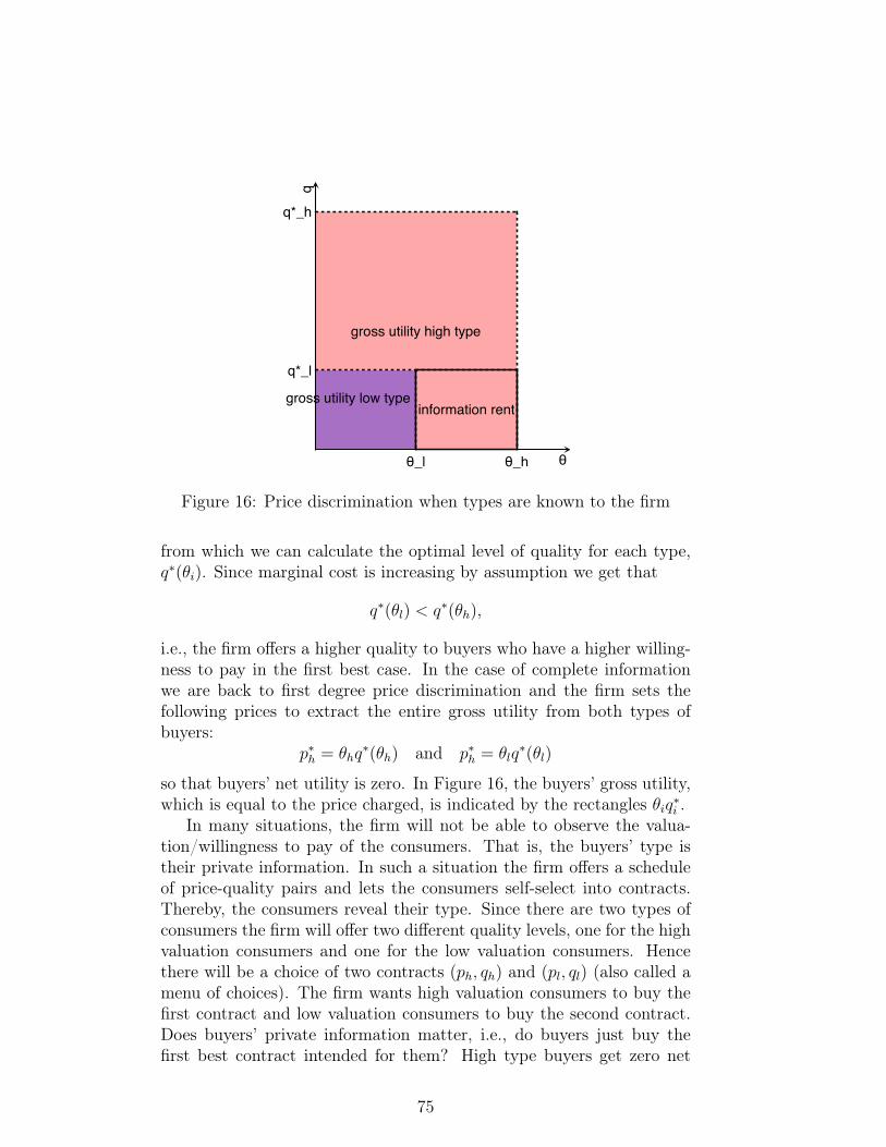
θ

q

q*_l

q*_h

θ_l θ_h

gross utility high type

gross utility low typeinformation rent

Figure 16: Price discrimination when types are known to the firm

from which we can calculate the optimal level of quality for each type,q∗(θi). Since marginal cost is increasing by assumption we get that

q∗(θl) < q∗(θh),

i.e., the firm offers a higher quality to buyers who have a higher willing-ness to pay in the first best case. In the case of complete informationwe are back to first degree price discrimination and the firm sets thefollowing prices to extract the entire gross utility from both types ofbuyers:

p∗h = θhq∗(θh) and p∗h = θlq

∗(θl)

so that buyers’ net utility is zero. In Figure 16, the buyers’ gross utility,which is equal to the price charged, is indicated by the rectangles θiq∗i .

In many situations, the firm will not be able to observe the valua-tion/willingness to pay of the consumers. That is, the buyers’ type istheir private information. In such a situation the firm offers a scheduleof price-quality pairs and lets the consumers self-select into contracts.Thereby, the consumers reveal their type. Since there are two types ofconsumers the firm will offer two different quality levels, one for the highvaluation consumers and one for the low valuation consumers. Hencethere will be a choice of two contracts (ph, qh) and (pl, ql) (also called amenu of choices). The firm wants high valuation consumers to buy thefirst contract and low valuation consumers to buy the second contract.Does buyers’ private information matter, i.e., do buyers just buy thefirst best contract intended for them? High type buyers get zero net

75

utility from buying the high quality contract, but positive net utility ofθhq∗(θl)− pl > 0. Hence, high type consumers have an incentive to pose

as low quality consumers and buy the contract intended for the low type.This is indicated in Figure 16 as “information rent,” i.e., an increase inhigh type buyers’ net utility due to asymmetric information.

The firm, not knowing the consumers’ type, however, can make thelow quality bundle less attractive to high type buyers by decreasing qlor make the high quality contract more attractive by increasing qh ordecreasing ph. The firm’s profit maximization problem now becomes

maxph,pl,qh,ql

α (ph − c(qh)) + (1− α) (pl − c(ql)) . (43)

There are two type of constraints. The consumers have the option ofwalking away, so the firm cannot demand payment higher than the valueof the object. That is, we must have

θhqh − ph≥ 0 (44)θlql − pl≥ 0. (45)

These are known as the individual rational (IR) or participation con-straints that guarantee that the consumers are willing to participate inthe trade. The other type of constraints are the self-selection or incentivecompatibility (IC) constraints

θhqh − ph≥ θhql − pl (46)θlql − pl≥ θlqh − ph, (47)

which state that each consumer type prefers the menu choice intendedfor him to the other contract. Not all of these four constraints can bebinding, because that would determine the optimal solution of pricesand quality levels. The IC for low type (47) will not binding becauselow types have no incentive to pretend to be high types: they wouldpay a high price for quality they do not value highly. On the otherhand high type consumers’ IR (44) will not be binding either becausewe argued above that the firm has to incentivize them to pick the highquality contract. This leaves constraints (45) and (46) as binding andwe can solve for the optimal prices

pl = θlql

using constraint (45) and

ph = θh(qh − ql) + θlql

76

using constraints (45) and (46). Substituting the prices into the profitfunction (43) yields

maxqh,ql

α [θh(qh − ql) + θlql − c(qh)] + (1− α) (θlql − c(ql)) .

The FOC for qh is simply

α (θh − c′(qh)) = 0,

which is identical to the FOC in the first best case. Hence, the firmoffers the high type buyers their first best quality level q∗R(θh) = q∗(θh).The FOC for ql is

α(θl − θh) + (1− α) (θl − c′(ql)) = 0,

which can be rewritten as

θl − c′(ql)−α

1− α(θl − θh) = 0.

The third term on the LHS, which is positive, is an additional costthat arises because the firm has to make the low quality contract lessattractive for high type buyers. Because of this additional cost we getthat q∗R(θl) < q∗(θl): the the quality level for low types is lower thanin the first best situation. This is depicted in Figure . The low typeconsumers’ gross utility and the high type buyers’ information rent aredecreased, but The optimal level of quality offered to low type buyers isdecreasing in the fraction of high type consumer α:

dq∗R(θl)

dα< 0

since the more high types there are the more the firm has to make thelow quality contract unattractive to them.

This analysis indicates some important results about second degreeprice discrimination:

1. The low type receives no surplus.

2. The high type receives a positive surplus of ql(θh − θl). This isknown as an information rent, that the consumer can extract be-cause the seller does not know his type.

3. The firm should set the efficient quality for the high valuation type.

4. The firm will degrade the quality for the low type in order to lowerthe rents the high type consumers can extract.

77

13 Auctions

Auctions are an important application of games of incomplete informa-tion. There are many markets where goods are allocated by auctions.Besides obvious examples such as auctions of antique furniture thereare many recent application. A leading example is Google’s sponsoredsearch auctions. Google matches advertiser to readers of websites andauctions advertising space according to complicated rules.

Consider a standard auction with I bidders, and each bidder i from1 to I has a valuation vi for a single object which is sold by the selleror auctioneer. If the bidder wins the object at price pi then he receivesutility vi − pi. Losing bidders receive a payoff or zero. The valuationis often the bidder’s private information so that we have to analyze theuncertainty inherent in such auctions. This uncertainty is captured bymodelling the bidders’ valuations as draws from a random distribution:

vi ∼ F (vi).

We assume that bidders are symmetric, i.e., their valuations come fromthe same distribution, and we let bi denote the bid of player i.

There are many possible rules for auctions. They can be either sealedbid or open bid. Examples of sealed bid auctions are the first priceauction (where the winner is the bidder with the highest bid and theypay their bid), and the second price auction (where the bidder withthe highest bid wins the object and pays the second highest bid as aprice). Open bid auctions include English auctions (the auctioneer setsa low price and keeps increasing the price until all but one player hasdropped out) and the Dutch auction (a high price is set and the priceis gradually lowered until someone accepts the offered price). Anothertype of auction is the Japanese button auction, which resembles an openbid ascending auction, but every time the price is raised all bidders haveto signal their willingness to increase their bid. Sometimes, bidders holddown a button as long as they want to increase their bid and releasewhen they want to exit the auction.

Let’s think about the optimal bidding strategy in a Japanese buttonauction, denotes by bi(vi) = ti, where ti = pi is the price the winningbidder pays for the good. At any time, the distribution of valuations,F , the number of remaining bidders are known to all players. As longas the price has not reached a bidder’s valuation it is optimal for himto keep the button pressed because he gets a positive payoff if all otherplayers exit before the price reaches his valuation. In particular, thebidder with the highest valuation will wait longest and therefore receivethe good. He will only have to pay the second highest bidder’s valuation,

78

however, because he should release the button as soon as he is the onlyone left. At that time the price will have exactly reached the secondhighest valuation. Hence, it is optimal for all bidders to bid their truevaluation. If the price exceeds vi they release the button and get 0 andthe highest valuation bidder gets a positive payoff. In other words, theoptimal strategy is

b∗i (vi) = vi.

What if the button auction is played as a descending auction instead?Then it is no longer optimal to bid one’s own valuation. Instead, b∗i (vi) <vi because only waiting until the price reaches one’s own valuation wouldmean that there might be a missed chance to get a strictly positive payoff.

In many situations (specifically when the other players’ valuationsdoes not affect your valuation) the optimal behavior in a second priceauction is equivalent to an English auction, and the optimal behaviourin a first price auction is equivalent to a Dutch auction. This providesa motivation for considering the second price auction which is strategi-cally very simple, since the English auction is commonly used. It’s themechanism used in the auction houses, and is a good first approximationhow auctions are run on eBay.

How should people bid in a second price auction? Typically a givenbidder will not know the bids/valuations of the other bidders. A nicefeature of the second price auction is that the optimal strategy is verysimple and does not depend on this information: each bidder should bidtheir true valuation.

Proposition 13.1. In a second price auction it is a Nash Equilibriumfor all players to bid their valuations. That is b∗i = vi for all i is a NashEquilibrium.

Proof. Without loss of generality, we can assume that player 1 has thehighest valuation. That is, we can assume v1 = maxi{vi}. Similarly, wecan assume without loss of generality that the second highest valuationis v2 = maxi>1{vi}. Define

µi(vi, bi, b−i) =

{vi − pi, if b1 = maxj{bj}

0, otherwise

}to be the surplus generated from the auction for each player i. Thenunder the given strategies (b = v)

µi(vi, vi, v−i) =

{v1 − v2, i = 10, otherwise

}So we want to show that no bidder has an incentive to deviate.

79

First we consider player 1. The payoff from bidding b1 is

µ1(v1, b1, v−1) =

{v1 − v2, if b1 > v2

0, otherwise

}≤ v1 − v2 = µ1(v1, v1, v−1)

so player 1 cannot benefit from deviating.Now consider any other player i > 1. They win the object only if

they bid more than v1 and would pay v1. So the payoff from bidding b1

isµi(vi, bi, v−i) =

{vi − v1, if bi > v1

0, otherwise

}≤ 0 = µi(vi, vi, v−i)

since vi − v1 ≤ 0. So player i has no incentive to deviate either.We have thus verified that all players are choosing a best response,

and so the strategies are a Nash Equilibrium.

Note that this allocation is efficient. The bidder with the highestvaluation gets the good.

Finally, we consider a first price sealed bid auction. There, we willsee that it is optimal for bidders to bid below their valuation, b∗i (vi) < vi,a strategy called bid shedding. Bidder i’s expected payoff is

maxbi

(vi − bi) Pr(bi > bj for all j 6= i) + 0 Pr(bi < max{bj} for all j 6= i).

(48)Consider the bidding strategy

bi(vi) = cvi

i.e., bidders bid a fraction of their true valuation. Then, if all playersplay this strategy,

Pr(bi > bj) = Pr(bi > cvj) = Pr

(vj <

bic

). (49)

With valuations having a uniform distribution on [0, 1], (49) becomes

Pr

(vj <

bic

)=bic

and (48) becomes

maxbi

(vi − bi)bic

+ 0

with FOCvi − 2bi

c= 0

80

orb∗i =

vi2.

Hence, we have verified that the optimal strategy is to bid a fraction ofone’s valuation, in particular, c = 1

2.

Typed by Richard Van Weelden (2007) and Vincent Pohl (2010)

81