1

INTERIM ANNUAL REPORT (FY 2016)

1. ADMINISTRATIVE

Date of Report: November 1, 2016

Period of Time Covered by Report: April 2015 – September 2016

Project Title: Impacts of Drought on Southwestern Cutthroat Trout: Influences of Changes in

Discharge and Stream Temperature on the Persistence across a Sub-set of Rio Grande Cutthroat

Trout Populations

Agreement Number: G15AC00263

Investigators: Colleen A. Caldwell, Ph.D., U.S. Geological Survey, New Mexico Cooperative

Fish and Wildlife Research Unit, 2980 South Espina Street, Knox Hall Room 132, Las Cruces,

New Mexico 88003; 575-646-8126; ccaldwel@usgs.gov

Brock Huntsman, Ph.D., Department of Fish, Wildlife and Conservation Ecology, New Mexico

State University, 2980 South Espina Street, Knox Hall Room 132, Las Cruces, New Mexico

88003; 575-646-6259; brockh12@nmsu.edu

Abigail Lynch, Ph.D., U.S. Geological Survey, National Climate Change and Wildlife Science

Center, 12201 Sunrise Valley Drive, MS-516, Room 2A225B, Reston, Virginia 20192;

ajlynch@usgs.gov

Bonnie Myers, U.S. Geological Survey, National Climate Change and Wildlife Science Center,

12201 Sunrise Valley Drive, MS-516, Room 2A105, Reston, Virginia 20192; bjmyers@usgs.gov

Funding Source and Project Timeline: U.S. Geological Survey, National Climate Change and

Wildlife Science Center (07/15/2015 – 09/30/2018; however, a no-cost time extension will be

requested due to the delay in recruiting and hiring of Dr. Huntsman)

2. PURPOSE AND OBJECTIVES

The primary goal of the study is to assess the likelihood and project the impacts of drought on a

subset of Rio Grande Cutthroat Trout (Oncorhynchus clarkii virginalis, RGCT) populations.

This work will provide insight into RGCT persistence under anticipated environmental and

biological pressures (e.g., drought, temperature, competition). Specific study objectives will be

to (1) empirically assess the effects of seasonal stream temperature and discharge on vital rates:

apparent survival, growth, recruitment; and (2) model drought effects on the persistence of

RGCT populations. The second objective includes two sub-objectives: a) model stream

discharge, intermittency, and temperature in occupied RGCT streams under projected drought

conditions and b) evaluate how drought conditions will alter population vital rates and

persistence of these populations.

Tasks associated with the first objective began shortly after the arrival of Dr. Huntsman at New

Mexico State University (February 2016). Dr. Huntsman noted that Objective 1 described the

selection of only three RGCT populations. His recommendation was to increase the number of

2

populations from three to at least eight populations to appropriately model vital rates (see Table

1). These eight populations should encompass a combination of environmental and biological

pressures. Although newly developed models can identify a subset of important vital rates via

count data through advancements in modeling software and computing power, these models lack

predictive power when compared to empirical data made available via capture-mark-recapture

methodologies. This equates to a complete block design in an analysis of variance framework

(Table 1). For example, three factors that influence RGCT vital rates would require at least eight

populations to capture all combinations of these factors (assuming only two fates of each factor:

drought vs. no drought). In addition, a much more robust sampling effort would be needed to

predict vital rates throughout the RGCT range. However, acquiring the needed capture-mark-

recapture data would be logistically impossible. This problem can be ameliorated by

incorporating an integrated population model that combines capture-mark-recapture data with

count data to estimate vital rates across sampling locations. For the capture-mark-recapture

component of the study, site selection is imperative. In addition, these locations must also

support a robust RGCT population to result in a reasonable number of recaptures each sampling

period (three seasons per year for three years).

A meeting with state biologists of the New Mexico Department of Game and Fish (NMDGF)

resulted in recommendations and eventual approval of the State Collection Permit (authorization

# 3033, 4/5/2016) of RGCT populations of importance. In addition, approval was granted to

obtain access to the RGCT database (not publically available) which identifies core RGCT

populations, known RGCT distributions throughout New Mexico and Colorado, genetic

structure, estimated population sizes, potential barrier locations, and presence of invasive trout.

3. ORGANIZATION AND APPROACH

Study Stream Selection and Sample Collection: Study streams were chosen based on three

criteria: (1) risk of the maximum weekly average temperature (MWAT) exceeding the 30-day

ultimate upper incipient lethal temperature for juvenile RGCT (21.7oC, Ziegler et al. 2013), (2)

presence or absence of invasive trout in the drainage, and (3) history of intermittency (see Table

1). All sample reaches were established above fish barriers to insure sufficient numbers of RGCT

were encountered for mark-recapture analysis. Therefore, invasive trout were not anticipated to

be encountered, however, brown trout are common above the barrier of one of the study streams

(Columbine Creek). Rio Grande Cutthroat Trout were sampled from all eight study streams in

the spring (5/4/2016-6/14/2016), summer (7/24/2016-8/10/2016), and fall (9/30/2016-10/9/2016)

(Figure 1, Table 2).

During each sampling period, RGCT were captured via triple pass depletion sampling with a

backpack electrofishing unit, although equipment failure resulted in 1 or 2 passes at a subset of

study streams during the summer (n = 4) and fall (n = 1) collections. During each survey, block

nets were anchored to the upper and lower ends of a 300 m segment of stream for depletion

surveys. Additionally, six 50m reaches within each 300 m study stream were delineated so fish

could be processed and released near their point of capture. This also allowed for tracking

potential fish movement at a spatial resolution of approximately 50 m. Upon capture, all fish

were measured for length (fork and total lengths, ±1 mm) and weight (±0.1 g). Additionally, fish

greater than 80 mm total length (TL) were implanted with a passive integrated transponder (PIT)

tag if they did not already possess a tag (Table 3). Lastly, diets from five large (≥115 mm TL)

3

and five small (<115 mm TL) RGCT size-classes were collected using gastric lavage for diet

identification. Unfortunately, no information exists on size-at-maturity for RGCT. Information

on size-at-maturity for Yellowstone Cutthroat Trout (O. c. bouvieri) does exist, where

Yellowstone Cutthroat Trout mature at approximately 2-3 years at 100-150mm total length

(Meyer et al. 2003). Therefore, the two size-classes defined here were based on RGCT von

Bertalanffy longevity models developed from otoliths collected by NMDGF, with a size cutoff at

an age of 2.5 years.

Water Quality: Water samples were collected from each study stream to characterize total

alkalinity and total hardness (mg/L as CaCO3). Water quality was collected using a HACH meter

to obtain instantaneous water temperature (oC), dissolved oxygen concentration (mg/L),

conductivity (µS/cm), and pH. Lastly, stream discharge was estimated at each study site using

the area-velocity approach (HACH digital flow meter; ft3/sec).

To monitor stream temperature and intermittency, two ProV2 temperature loggers as well as two

intermittency loggers were deployed in two separate pools and riffles within each study stream.

The intermittency loggers are a modified Hobo Pendant data logger (ONSET, Inc) that enables

simultaneous collection of high-resolution water temperature and electrical resistance (Chapin et

al. 2014). This single, multi-functional sensor can reliably collect both the temperature and flow

within a stream from which one can infer wet versus dry conditions.

Drift and Benthic Macroinvertebrates: Prior to electrofishing, macroinvertebrate drift and

benthic samples were collected within each study stream. While not a part of the original scope

of work, aquatic invertebrates provide the needed insight to characterize energetics and trophic

basis of production in response to temperature challenges and intermittency. Drift

macroinvertebrates were collected mid-day between 9:00 and 14:00 (Grant and Noakes 1987).

Three replicate drift samples were collected with drift nets (width = 44 cm, depth = 27 cm; 250

µm mesh) deployed at three independent riffles (separated by a non-riffle channel unit). Benthic

macroinvertebrates were similarly collected from three independent pools and three independent

riffles using a benthic Hess sampler (diameter = 33 cm; 250 µm mesh). All samples were

returned to the laboratory where they will be processed by splitting into 1 mm and 250 µm

fractions (for large samples). All macroinvertebrates from the coarse fraction (>1 mm) will be

separated from organic and inorganic material and identified to the lowest taxonomic unit

possible (typically genus). The fine fraction (1 mm-250 µm) will be split to a 1/8th fraction using

a Folsom plankton splitter, and all macroinvertebrates will be identified. For small samples, the

entire sample will be identified.

Fish Habitat: In the summer (July 6-9), habitat was classified within each 50 m segment of each

study stream using a thalweg profile (Petty et al. 2003, 2005). Every three meters for the entire

300 m study reach, a habitat measurement was taken within the thalweg. Measurements taken at

each point along the thalweg included 60% velocity, substrate size (mm), depth (cm), distance to

fish cover (cm), and fish cover type (e.g., rock, woody debris, undercut). All substrate was

grouped into substrate categories based on the Wolman pebble count methodologies.

Additionally, wetted width (m) and canopy cover (via a densiometer) was recorded at every 5th

measurement. Lastly, channel units (i.e., pool, riffle, run, glide, and cascade) were identified and

the slope (%) of the channel unit was measured with a clinometer.

4

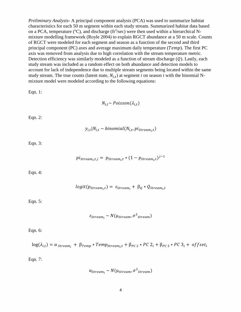
Preliminary Analysis- A principal component analysis (PCA) was used to summarize habitat

characteristics for each 50 m segment within each study stream. Summarized habitat data based

on a PCA, temperature (oC), and discharge (ft3/sec) were then used within a hierarchical N-

mixture modelling framework (Royle 2004) to explain RGCT abundance at a 50 m scale. Counts

of RGCT were modeled for each segment and season as a function of the second and third

principal component (PC) axes and average maximum daily temperature (𝑇𝑒𝑚𝑝). The first PC

axis was removed from analysis due to high correlation with the stream temperature metric.

Detection efficiency was similarly modeled as a function of stream discharge (𝑄). Lastly, each

study stream was included as a random effect on both abundance and detection models to

account for lack of independence due to multiple stream segments being located within the same

study stream. The true counts (latent state, 𝑁𝑖,𝑡) at segment i on season t with the binomial N-

mixture model were modeled according to the following equations:

Eqn. 1:

𝑁𝑖,𝑡~ 𝑃𝑜𝑖𝑠𝑠𝑜𝑛(𝜆𝑖,𝑡)

Eqn. 2:

𝑦𝑖,𝑡|𝑁𝑖,𝑡 ~ 𝑏𝑖𝑛𝑜𝑚𝑖𝑎𝑙(𝑁𝑖,𝑡, 𝑝𝑖𝑆𝑡𝑟𝑒𝑎𝑚𝑖,𝑡)

Eqn. 3:

𝑝𝑖𝑆𝑡𝑟𝑒𝑎𝑚𝑖,𝑡,𝑗 = 𝑝𝑆𝑡𝑟𝑒𝑎𝑚𝑖,𝑡 ∗ (1 − 𝑝𝑆𝑡𝑟𝑒𝑎𝑚𝑖,𝑡)𝑗−1

Eqn. 4:

𝑙𝑜𝑔𝑖𝑡(𝑝𝑆𝑡𝑟𝑒𝑎𝑚𝑖,𝑡) = 𝜀𝑆𝑡𝑟𝑒𝑎𝑚𝑖+ β𝑄 ∗ 𝑄𝑆𝑡𝑟𝑒𝑎𝑚𝑖,𝑡

Eqn. 5:

𝜀𝑆𝑡𝑟𝑒𝑎𝑚𝑖 ~ 𝑁(µ𝑆𝑡𝑟𝑒𝑎𝑚, 𝜎2

𝑆𝑡𝑟𝑒𝑎𝑚)

Eqn. 6:

log(𝜆𝑖,𝑡) = α 𝑆𝑡𝑟𝑒𝑎𝑚𝑖 + β𝑇𝑒𝑚𝑝 ∗ 𝑇𝑒𝑚𝑝𝑆𝑡𝑟𝑒𝑎𝑚𝑖,𝑡 + β𝑃𝐶 2 ∗ 𝑃𝐶 2𝑖 + β𝑃𝐶 3 ∗ 𝑃𝐶 3𝑖 + 𝑜𝑓𝑓𝑠𝑒𝑡𝑖

Eqn. 7:

α𝑆𝑡𝑟𝑒𝑎𝑚𝑖 ~ 𝑁(µ𝑆𝑡𝑟𝑒𝑎𝑚, 𝜎2

𝑆𝑡𝑟𝑒𝑎𝑚)

5

Where detection efficiency (𝑝) was estimated for each stream (streami), electrofishing pass (1, 2,

or 3) represented by j, and season t as a function of discharge Q. Stream was also modelled as a

random effect on both detection efficiency (𝜀𝑆𝑡𝑟𝑒𝑎𝑚𝑖) as well as RGCT counts (α𝑆𝑡𝑟𝑒𝑎𝑚). We

included an offset (log of segment length) when modeling RGCT counts to account for unequal

length of some stream segments.

A Bayesian approach with Markov chain Monte Carlo (MCMC) methods in JAGS (Plummer

2013) was used within the R programing language (R Development Core Team 2015) with the

“jagsUI” package (Kellner 2015) to construct the N-mixture model. The Bayesian analysis was

run with three chains, a chain length of 100,000 burn-in of 50,000, and a thinning value of 100.

Model convergence was confirmed by Gelman and Rubin convergence diagnostics (�̂� < 1.1,

Gelman and Rubin 1992). Minimally informative priors were used for all regression

coefficients, β ~ N(0,1).

Growth rates were estimated for RGCT as the difference in log transformed total lengths (TL)

between initial capture and recapture divided by the number of days between captures ([log(TL

recapture) – log(TL initial capture)]/days). Total lengths were transformed for growth data

because fish growth is typically non-linear. Growth rates were estimated for the two size-classes

and during the summer and fall intervals, since fish were first captured in the spring.

4. RESULTS (PRELIMINARY)

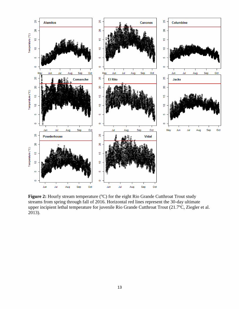
Stream Temperature and Fish Habitat: Stream temperature loggers identified thermal profiles in

four of the eight study streams exceeded the ultimate upper incipient lethal temperature of 21.7ºC

for juvenile RGCT (Ziegler et al. 2013; Figure 2). The warmest streams on average were the two

grassland streams (Comanche and Vidal), with Cañones and El Rito being the next warmest. The

remaining four streams (Vidal, Alamitos, Jacks, and Powderhouse) never exceeded the upper

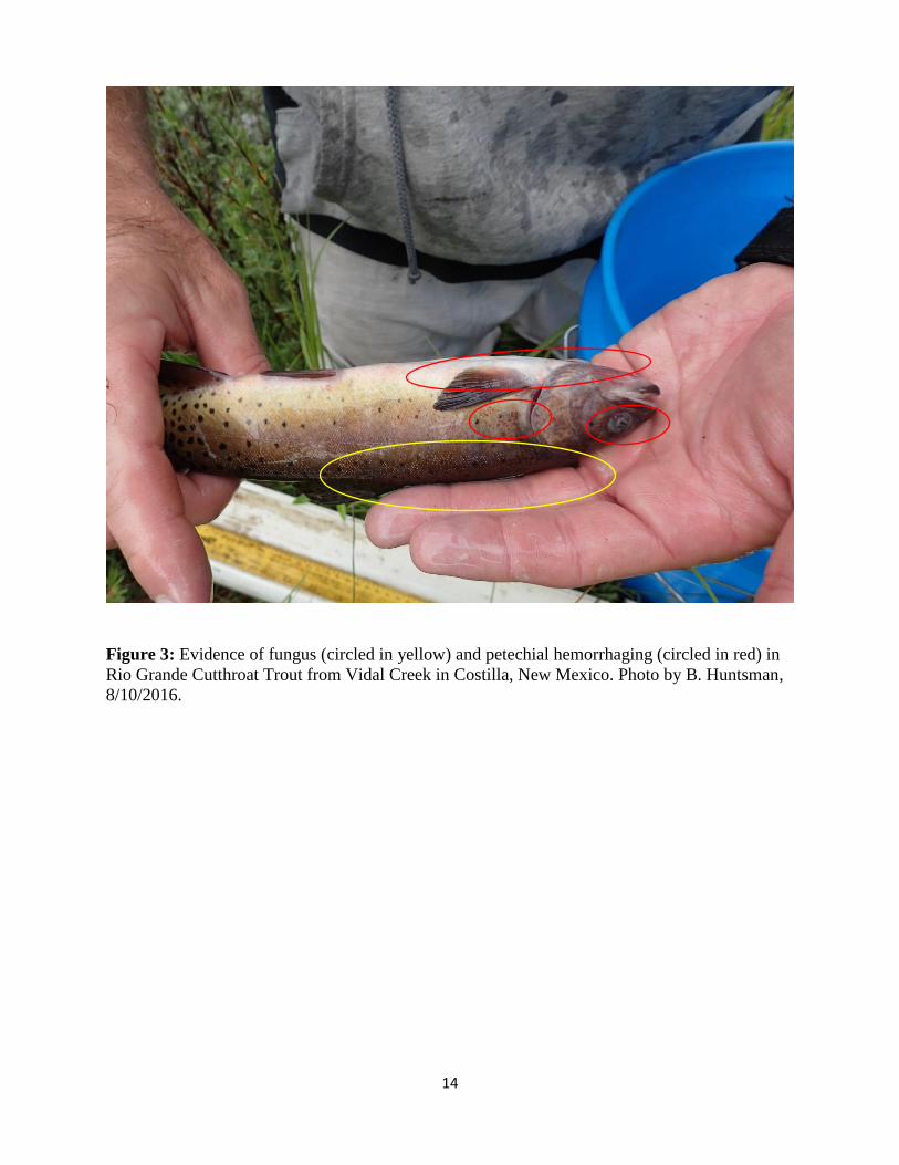
incipient temperature. Interestingly, the four streams that exceeded this upper stressful thermal

limit also contained fish with fungal infections (Figure 3). While anecdotal, these observations

suggest these populations were immunocompromised likely due to stressful thermal limits and

warrants further investigations (Table 3).

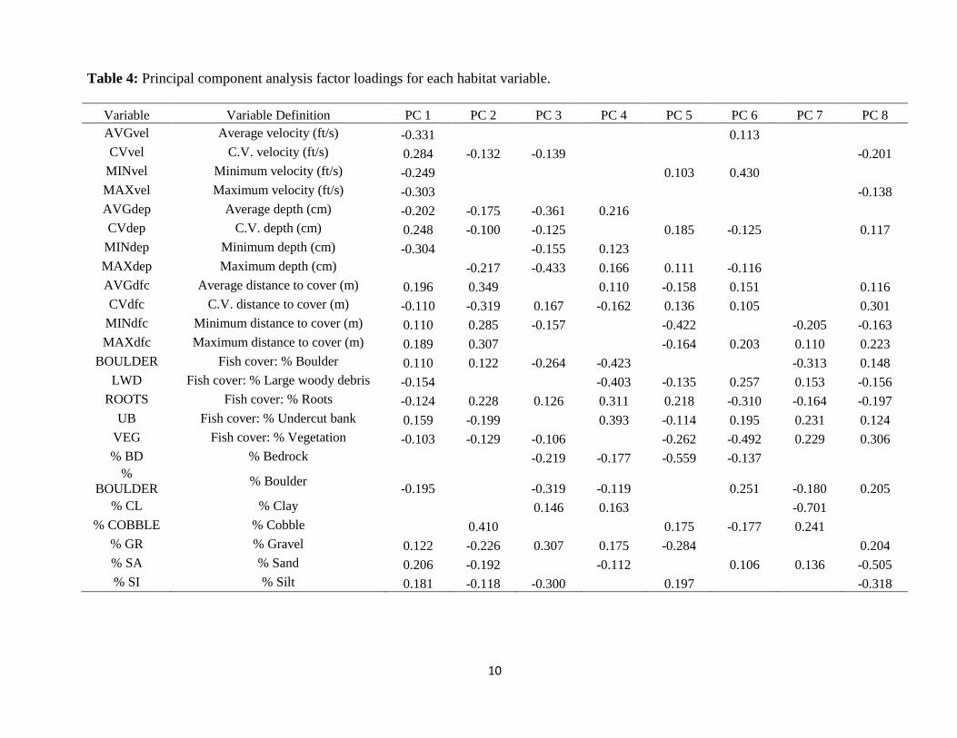
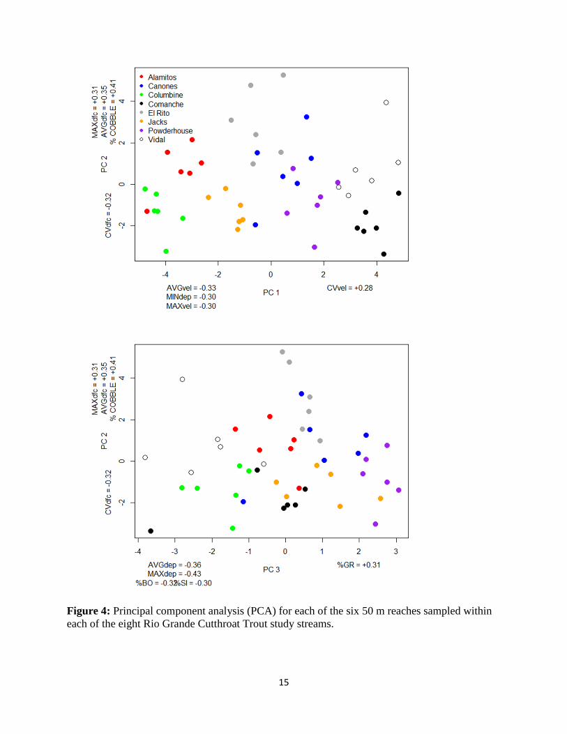
The first three components of the PCA accounted for 55% of the variation in the habitat

variables. The first principal component axis (PC 1) separated sites by a stream velocity gradient,

where streams with greatest flows loaded strongly on the negative side of this axis (Figure 4,

Table 4). Columbine and Alamitos loaded strongly on the high velocity side of this axis, while

the two low gradient grassland streams (Vidal and Comanche) loaded strongest on the positive

side of PC 1. In contrast, PC 2 reflected a fish cover gradient, where streams with greater

distances between objects that could conceal RGCT loaded strongest on the positive side of this

axis. El Rito, Cañones, and Vidal had greater distances between fish cover objects compared to

Columbine, Powderhouse, Jacks, and Comanche. A third PC axis identified a stream depth

gradient, where the deepest sites with dominant substrates of silt and boulder loaded strongest in

the negative direction (Figure 4).

Fish Sampling, Movement, N-mixture Model, and Growth Rates: A total of 1,762 RGCT were

captured across the three sample collection dates. Of this total, 1,201 were tagged and 515

recaptures were encountered (Table 3). The highest number of RGCT captured was 541 from

Jacks, followed by 410 in Alamitos, and 298 in Powderhouse. The fewest number of fish

encountered was from Columbine (the only RGCT population sympatric with brown trout)

6

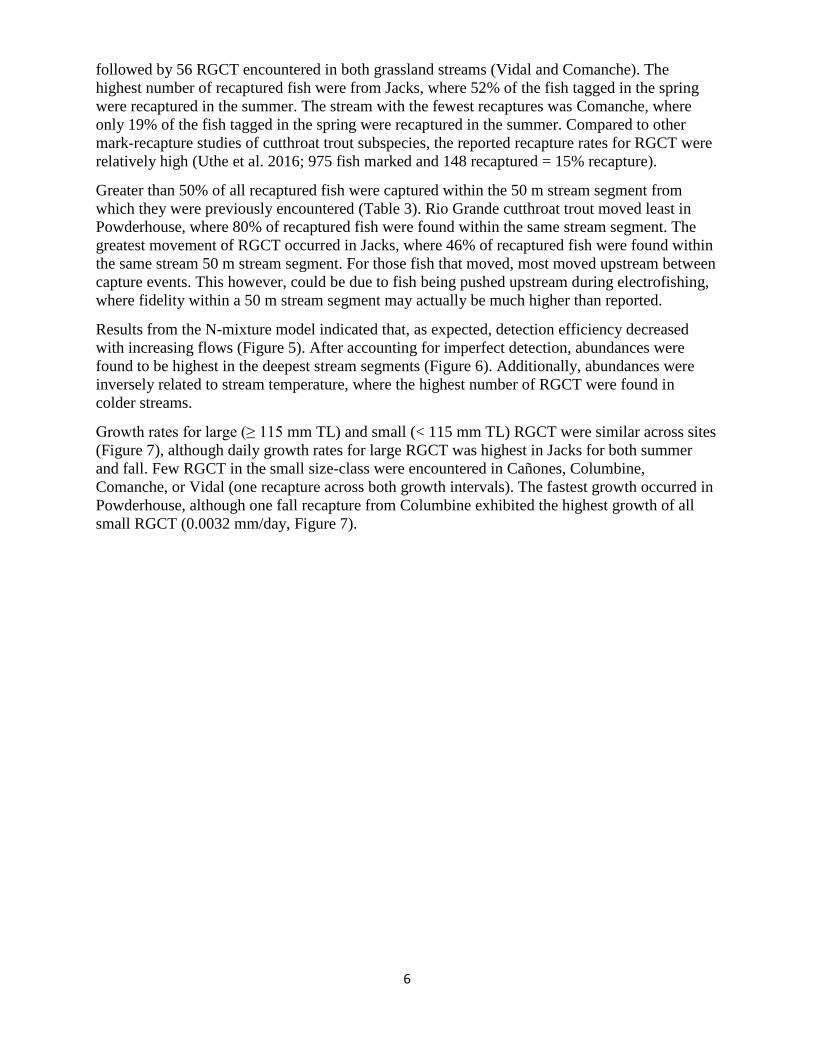
followed by 56 RGCT encountered in both grassland streams (Vidal and Comanche). The

highest number of recaptured fish were from Jacks, where 52% of the fish tagged in the spring

were recaptured in the summer. The stream with the fewest recaptures was Comanche, where

only 19% of the fish tagged in the spring were recaptured in the summer. Compared to other

mark-recapture studies of cutthroat trout subspecies, the reported recapture rates for RGCT were

relatively high (Uthe et al. 2016; 975 fish marked and 148 recaptured = 15% recapture).

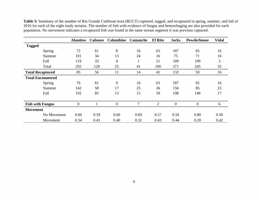
Greater than 50% of all recaptured fish were captured within the 50 m stream segment from

which they were previously encountered (Table 3). Rio Grande cutthroat trout moved least in

Powderhouse, where 80% of recaptured fish were found within the same stream segment. The

greatest movement of RGCT occurred in Jacks, where 46% of recaptured fish were found within

the same stream 50 m stream segment. For those fish that moved, most moved upstream between

capture events. This however, could be due to fish being pushed upstream during electrofishing,

where fidelity within a 50 m stream segment may actually be much higher than reported.

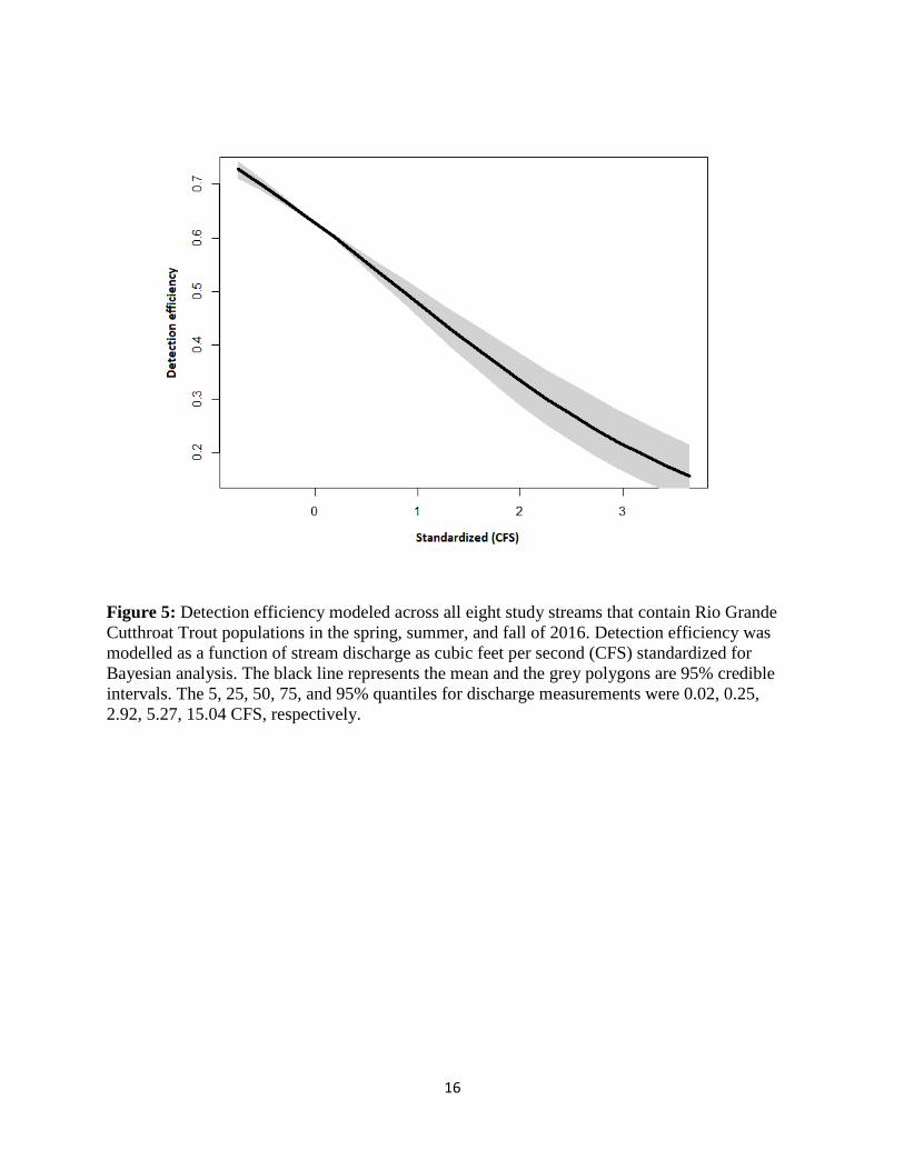
Results from the N-mixture model indicated that, as expected, detection efficiency decreased

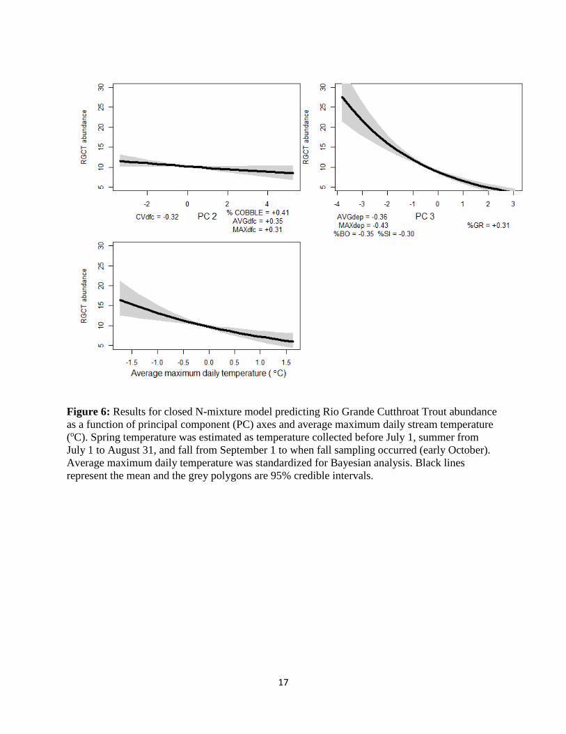
with increasing flows (Figure 5). After accounting for imperfect detection, abundances were

found to be highest in the deepest stream segments (Figure 6). Additionally, abundances were

inversely related to stream temperature, where the highest number of RGCT were found in

colder streams.

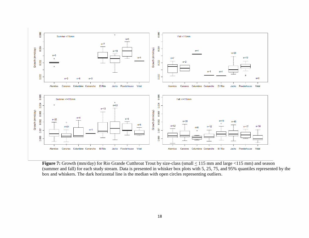
Growth rates for large (≥ 115 mm TL) and small (< 115 mm TL) RGCT were similar across sites

(Figure 7), although daily growth rates for large RGCT was highest in Jacks for both summer

and fall. Few RGCT in the small size-class were encountered in Cañones, Columbine,

Comanche, or Vidal (one recapture across both growth intervals). The fastest growth occurred in

Powderhouse, although one fall recapture from Columbine exhibited the highest growth of all

small RGCT (0.0032 mm/day, Figure 7).

7

Table 1: Nested design for study site selection based on history of thermal regimes, presence of

invasive trout within the drainage, and intermittency. A “Y” (yes) indicates the stream meets the

specified criterion and “N” (no) indicates the stream did not meet the criterion.

Watershed

Stream Name

Temperature

(MWAT>21.7ºC)

Invasive

Trout within

the Drainage

Intermittent

Rio Chama Cañones Y Y Y

Rio Chama El Rito Y Y N

Upper Rio Grande Comanche Y N Y

Upper Rio Grande Vidal Y N N

Upper Rio Grande Alamitos N N N

Pecos Jacks N N Y

Upper Rio Grande Columbine N Y N

Upper Rio Grande Powderhouse N Y Y

8

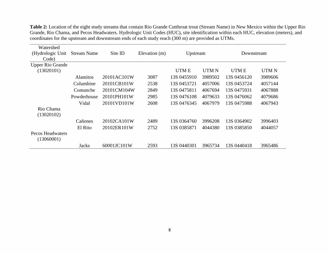
Table 2: Location of the eight study streams that contain Rio Grande Cutthroat trout (Stream Name) in New Mexico within the Upper Rio

Grande, Rio Chama, and Pecos Headwaters. Hydrologic Unit Codes (HUC), site identification within each HUC, elevation (meters), and

coordinates for the upstream and downstream ends of each study reach (300 m) are provided as UTMs.

Watershed

(Hydrologic Unit

Code)

Stream Name

Site ID

Elevation (m)

Upstream

Downstream

Upper Rio Grande

(13020101) UTM E UTM N UTM E UTM N

Alamitos 20101AC101W 3087 13S 0455910 3989502 13S 0456120 3989606

Columbine 20101CB101W 2538 13S 0453721 4057006 13S 0453724 4057144

Comanche 20101CM104W 2849 13S 0475811 4067694 13S 0475931 4067888

Powderhouse 20101PH101W 2985 13S 0476108 4079633 13S 0476062 4079686

Vidal 20101VD101W 2608 13S 0476345 4067979 13S 0475988 4067943

Rio Chama

(13020102)

Cañones 20102CA101W 2489 13S 0364760 3996208 13S 0364902 3996403

El Rito 20102ER101W 2752 13S 0385871 4044380 13S 0385850 4044057

Pecos Headwaters

(13060001)

Jacks 60001JC101W 2593 13S 0440301 3965734 13S 0440418 3965486

9

Table 3: Summary of the number of Rio Grande Cutthroat trout (RGCT) captured, tagged, and recaptured in spring, summer, and fall of

2016 for each of the eight study streams. The number of fish with evidence of fungus and hemorrhaging are also provided for each

population. No movement indicates a recaptured fish was found in the same stream segment it was previous captured.

Alamitos Cañones Columbine Comanche El Rito Jacks Powderhouse Vidal

Tagged

Spring 72 61 8 16 63 187 65 16

Summer 101 34 13 24 16 75 71 16

Fall 119 33 4 1 21 109 109 3

Total 292 128 25 41 100 371 245 35

Total Recaptured 85 56 11 14 41 132 50 16

Total Encountered

Spring 76 61 9 16 63 187 65 16

Summer 142 58 17 25 36 156 85 23

Fall 192 85 13 15 59 198 148 17

Fish with Fungus 0 1 0 7 2 0 0 6

Movement

No Movement 0.66 0.59 0.60 0.69 0.57 0.56 0.80 0.58

Movement 0.34 0.41 0.40 0.31 0.43 0.44 0.20 0.42

10

Table 4: Principal component analysis factor loadings for each habitat variable.

Variable Variable Definition PC 1 PC 2 PC 3 PC 4 PC 5 PC 6 PC 7 PC 8

AVGvel Average velocity (ft/s) -0.331 0.113 CVvel C.V. velocity (ft/s) 0.284 -0.132 -0.139 -0.201

MINvel Minimum velocity (ft/s) -0.249 0.103 0.430 MAXvel Maximum velocity (ft/s) -0.303 -0.138

AVGdep Average depth (cm) -0.202 -0.175 -0.361 0.216 CVdep C.V. depth (cm) 0.248 -0.100 -0.125 0.185 -0.125 0.117

MINdep Minimum depth (cm) -0.304 -0.155 0.123 MAXdep Maximum depth (cm) -0.217 -0.433 0.166 0.111 -0.116 AVGdfc Average distance to cover (m) 0.196 0.349 0.110 -0.158 0.151 0.116

CVdfc C.V. distance to cover (m) -0.110 -0.319 0.167 -0.162 0.136 0.105 0.301

MINdfc Minimum distance to cover (m) 0.110 0.285 -0.157 -0.422 -0.205 -0.163

MAXdfc Maximum distance to cover (m) 0.189 0.307 -0.164 0.203 0.110 0.223

BOULDER Fish cover: % Boulder 0.110 0.122 -0.264 -0.423 -0.313 0.148

LWD Fish cover: % Large woody debris -0.154 -0.403 -0.135 0.257 0.153 -0.156

ROOTS Fish cover: % Roots -0.124 0.228 0.126 0.311 0.218 -0.310 -0.164 -0.197

UB Fish cover: % Undercut bank 0.159 -0.199 0.393 -0.114 0.195 0.231 0.124

VEG Fish cover: % Vegetation -0.103 -0.129 -0.106 -0.262 -0.492 0.229 0.306

% BD % Bedrock -0.219 -0.177 -0.559 -0.137 %

BOULDER % Boulder

-0.195 -0.319 -0.119 0.251 -0.180 0.205

% CL % Clay 0.146 0.163 -0.701 % COBBLE % Cobble 0.410 0.175 -0.177 0.241

% GR % Gravel 0.122 -0.226 0.307 0.175 -0.284 0.204

% SA % Sand 0.206 -0.192 -0.112 0.106 0.136 -0.505

% SI % Silt 0.181 -0.118 -0.300 0.197 -0.318

11

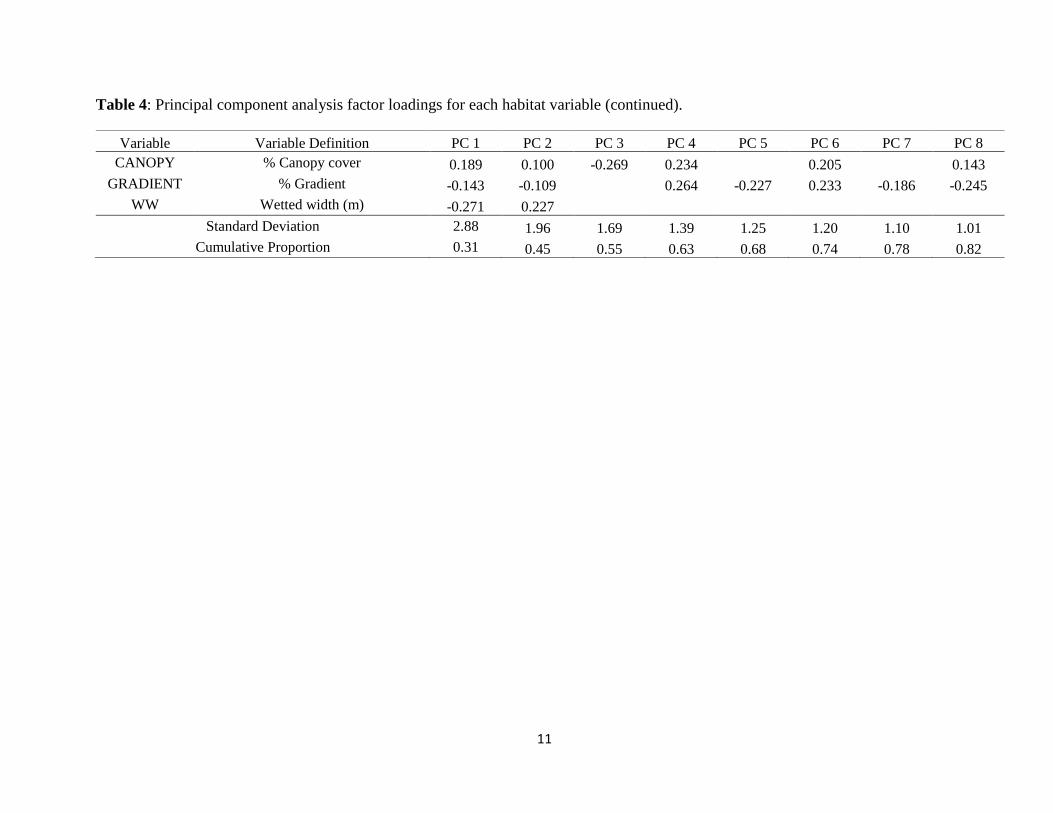
Table 4: Principal component analysis factor loadings for each habitat variable (continued).

Variable Variable Definition PC 1 PC 2 PC 3 PC 4 PC 5 PC 6 PC 7 PC 8

CANOPY % Canopy cover 0.189 0.100 -0.269 0.234 0.205 0.143

GRADIENT % Gradient -0.143 -0.109 0.264 -0.227 0.233 -0.186 -0.245

WW Wetted width (m) -0.271 0.227 Standard Deviation 2.88 1.96 1.69 1.39 1.25 1.20 1.10 1.01

Cumulative Proportion 0.31 0.45 0.55 0.63 0.68 0.74 0.78 0.82

12

Figure 1: Location of the eight Rio Grande Cutthroat Trout study streams within New Mexico.

Streams are located within the three watersheds (Pecos, Rio Chama, and Upper Rio Grande).

13

Figure 2: Hourly stream temperature (oC) for the eight Rio Grande Cutthroat Trout study

streams from spring through fall of 2016. Horizontal red lines represent the 30-day ultimate

upper incipient lethal temperature for juvenile Rio Grande Cutthroat Trout (21.7oC, Ziegler et al.

2013).

14

Figure 3: Evidence of fungus (circled in yellow) and petechial hemorrhaging (circled in red) in

Rio Grande Cutthroat Trout from Vidal Creek in Costilla, New Mexico. Photo by B. Huntsman,

8/10/2016.

15

Figure 4: Principal component analysis (PCA) for each of the six 50 m reaches sampled within

each of the eight Rio Grande Cutthroat Trout study streams.

16

Figure 5: Detection efficiency modeled across all eight study streams that contain Rio Grande

Cutthroat Trout populations in the spring, summer, and fall of 2016. Detection efficiency was

modelled as a function of stream discharge as cubic feet per second (CFS) standardized for

Bayesian analysis. The black line represents the mean and the grey polygons are 95% credible

intervals. The 5, 25, 50, 75, and 95% quantiles for discharge measurements were 0.02, 0.25,

2.92, 5.27, 15.04 CFS, respectively.

17

Figure 6: Results for closed N-mixture model predicting Rio Grande Cutthroat Trout abundance

as a function of principal component (PC) axes and average maximum daily stream temperature

(oC). Spring temperature was estimated as temperature collected before July 1, summer from

July 1 to August 31, and fall from September 1 to when fall sampling occurred (early October).

Average maximum daily temperature was standardized for Bayesian analysis. Black lines

represent the mean and the grey polygons are 95% credible intervals.

18

Figure 7: Growth (mm/day) for Rio Grande Cutthroat Trout by size-class (small < 115 mm and large <115 mm) and season

(summer and fall) for each study stream. Data is presented in whisker box plots with 5, 25, 75, and 95% quantiles represented by the

box and whiskers. The dark horizontal line is the median with open circles representing outliers.

19

Interesting Patterns and Interpretation: Our preliminary analyses indicate that habitat and

temperature play an important role in RGCT population dynamics. Populations within the two

grassland study streams (Comanche and Vidal) and the Cañones experienced thermal regimes in

excess of the published critical upper limit (~21.7ºC) and supported fewer fish than cooler

streams. We caution that with only one year of monitoring it is difficult to attribute lower

abundance to temperature related mortality as opposed to RGCT seeking thermal refugia, a

common behavior in salmonids. However, limited movement observed in this study and the

presence of immunocompromised fish in streams where temperatures exceed upper lethal limits

suggest temperatures are likely negatively impacting vital rates and warrant further study (i.e.,

survival).

Another interesting pattern observed from this preliminary analysis was that Columbine

supported the fewest RGCT. This is surprising since temperature regimes (Figure 2) and habitat

(Figure 3) within Columbine suggest population size should be relatively large based on

favorable conditions predicted from the N-mixture model. Specifically, temperature is well

below upper lethal limits and stream depth is among the deepest among study sites (PC 3).

However, RGCT counts in Columbine were consistently lower than all other study streams and

small RGCT were consistently absent from collections. Interestingly, this was the only stream in

the study that contained sympatric non-native trout (Brown Trout Salmo trutta). Although

surveys below barriers at these sites have not been conducted, it could provide a unique

“experimental manipulation” to tease out the impacts of invasive trout on RGCT population

dynamics.

A final interesting pattern from these preliminary analyses is that little separation in

instantaneous growth rates were observed across all sites. This was surprising given that the

populations experienced a range of stream temperatures and fish densities. However, the greatest

variability in growth among the populations occurred with the smaller size-class. This would be

expected since small salmonids are less likely to successfully compete for resources (e.g.,

foraging positions) compared to large salmonids. Unfortunately, few small fish were consistently

found in all streams limiting our sample size. The importance of density-dependence and

environmental factors (e.g. temperature) will be further explored with regression models as well

as investigating trophic basis of production, to determine the importance of such factors on

RGCT productivity.

5. NEXT STEPS

Timeline (April 2015-September 2019; no cost time extension) 3.5 years

Objective 1; Objective 2a; Objective 2b

Apr-2015 Establish cooperative agreement with New Mexico Cooperative Fish and

Wildlife Research Unit; begin project development through teleconferences.

Recommend site visits occur for all investigators.

Jan-2016 Hired post-doctoral research associate (Dr. Brock Huntsman) to oversee the

project.

20

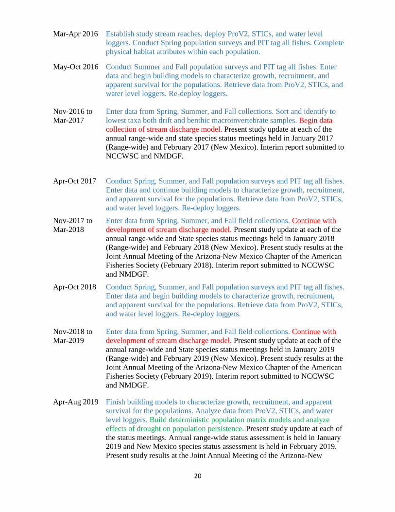
Mar-Apr 2016 Establish study stream reaches, deploy ProV2, STICs, and water level

loggers. Conduct Spring population surveys and PIT tag all fishes. Complete

physical habitat attributes within each population.

May-Oct 2016 Conduct Summer and Fall population surveys and PIT tag all fishes. Enter

data and begin building models to characterize growth, recruitment, and

apparent survival for the populations. Retrieve data from ProV2, STICs, and

water level loggers. Re-deploy loggers.

Nov-2016 to

Mar-2017

Enter data from Spring, Summer, and Fall collections. Sort and identify to

lowest taxa both drift and benthic macroinvertebrate samples. Begin data

collection of stream discharge model. Present study update at each of the

annual range-wide and state species status meetings held in January 2017

(Range-wide) and February 2017 (New Mexico). Interim report submitted to

NCCWSC and NMDGF.

Apr-Oct 2017 Conduct Spring, Summer, and Fall population surveys and PIT tag all fishes.

Enter data and continue building models to characterize growth, recruitment,

and apparent survival for the populations. Retrieve data from ProV2, STICs,

and water level loggers. Re-deploy loggers.

Nov-2017 to

Mar-2018

Enter data from Spring, Summer, and Fall field collections. Continue with

development of stream discharge model. Present study update at each of the

annual range-wide and State species status meetings held in January 2018

(Range-wide) and February 2018 (New Mexico). Present study results at the

Joint Annual Meeting of the Arizona-New Mexico Chapter of the American

Fisheries Society (February 2018). Interim report submitted to NCCWSC

and NMDGF.

Apr-Oct 2018 Conduct Spring, Summer, and Fall population surveys and PIT tag all fishes.

Enter data and begin building models to characterize growth, recruitment,

and apparent survival for the populations. Retrieve data from ProV2, STICs,

and water level loggers. Re-deploy loggers.

Nov-2018 to

Mar-2019

Enter data from Spring, Summer, and Fall field collections. Continue with

development of stream discharge model. Present study update at each of the

annual range-wide and State species status meetings held in January 2019

(Range-wide) and February 2019 (New Mexico). Present study results at the

Joint Annual Meeting of the Arizona-New Mexico Chapter of the American

Fisheries Society (February 2019). Interim report submitted to NCCWSC

and NMDGF.

Apr-Aug 2019 Finish building models to characterize growth, recruitment, and apparent

survival for the populations. Analyze data from ProV2, STICs, and water

level loggers. Build deterministic population matrix models and analyze

effects of drought on population persistence. Present study update at each of

the status meetings. Annual range-wide status assessment is held in January

2019 and New Mexico species status assessment is held in February 2019.

Present study results at the Joint Annual Meeting of the Arizona-New

21

Mexico Chapter of the American Fisheries Society (February 2019). Present

results to date at the XII Wild Trout Symposium, West Yellowstone,

Montana (July).

Sep-2019 Complete File Report. Complete and submit manuscript on the effects of

drought on population vital rates and persistence of Rio Grande cutthroat

trout population persistence.

6. OUTREACH

a. No articles or reports have been developed at this time; however, an RGCT otolith

manuscript is currently being developed with NMDGF.

b. No project-related presentations, seminars, or webinars have been developed at this time;

however, a presentation is planned for the 50th Joint Annual Meeting of the AZ/NM

American Fisheries Society and the New Mexico and Arizona Wildlife Societies

(February 2017).

c. This project is conducted through the partnership of New Mexico Department of Game

and Fish, U.S. Forest Service (Carson and Santa Fe National Forests), and local and

national interest groups such as Trout Unlimited (National Trout Unlimited and local

chapters such as the Gila/Rio Grande Chapter).

d. No websites have been created for data sharing at this time.

e. No other products such as databases, audio/video productions, or fact sheets has been

developed at this time.

7. PROFESSIONAL DEVELOPEMENT

a. A workshop on integrated population models was attended at Patuxent Wildlife Research

Center by Dr. Brock Huntsman (Aug. 1-5, 2016).

b. Educational outreach in the form of hiring graduate and undergraduate students to assist

with the project: Recruitment of Lauren Flynn to pursue her graduate research (M.S.

degree at NMSU) with the PIs of the project. Ms. Flynn will contribute towards the

project by way of addressing the effects that temperature and intermittency will have on

the energetics and secondary production of RGCT. Mr. Quintin Dean, undergraduate

senior in the Department of Fish, Wildlife and Conservation Ecology at NMSU, was

hired to participate in the project by assisting Dr. Huntsman with sorting and identifying

drift and benthic macroinvertebrates. The majority of Mr. Dean’s wages will be paid by

an NMSU scholarship.

8. BUDGET

As of 17 October 2016, project balance: $172,038 (total funding $257,878). The

agreement was modified 8/8/2016 to add $20,700 for Ms. Lauren Flynn, graduate

research assistant, to assist with the project and to pursue her MS degree. Expenditures

from inception of project are the following (do not include 15% indirect costs): Payroll

(includes 32% fringe) $37,575.94; Travel $3,487.91; Materials and Supplies $9,413.04.

22

Literature Cited

Chapin TP, Todd AS, Zeigler MP (2014) Robust, low‐ cost data loggers for stream temperature,

flow intermittency, and relative conductivity monitoring. Water Resources Research.

50:6542-6548.

Coleman MA, Fausch KD (2007) Cold summer temperature limits recruitment of age-0 cutthroat

trout in high-elevation Colorado streams. Transactions of the American Fisheries Society.

136:1231-1244.

Gelman A, Rubin DB (1992) Inference from iterative simulation using multiple sequences.

Statistical Science 7:457-511.

Grant JWA, Noakes DLG (1987) Movers and stayers: Foraging tactics of young-of-the-year

brook charr, Salvelinus fontinalis. Journal of Animal Ecology. 56:1001-1013.

Kellner K (2015) jagsUI: a wrapper around rjags to streamline JAGS analyses. R package

version, 1(1).

Petty JT, Freund J, Lamothe PJ, Mazik PM (2003) Quantifying the microhabitat characteristics

of hydraulic channel units in the upper Shavers Fork basin. Proceedings of the Annual

Conference South-eastern Association of Fish and Wildlife Agencies. 55:81-94.

Petty JT, Lamothe PJ, Mazik PM (2005) Spatial and seasonal dynamics of brook trout

populations inhabiting a central Appalachian watershed. Transactions of the American

Fisheries Society. 134:572-587.

Plummer M (2013). Just Another Gibbs Sampler (JAGS) Software.

Royle JA (2004) N-mixture models for estimating population size from spatially Replicated

counts. Biometrics 60:108–115.

Uthe P, Al-Chokhachy R, Zale AV, Shepard BB, McMahon TE, Stephens T (2016) Life history

characteristics and vital rates of Yellowstone Cutthroat Trout in two headwater basins. North

American Journal of Fisheries Management 36:1240-1253.

Zeigler MP, Brinkman SF, Caldwell CA, Todd AS, Recsetar MS, Bonar SA (2013) Upper

thermal tolerances of Rio Grande cutthroat trout under constant and fluctuating temperatures.

Transactions of the American Fisheries Society. 142:1395-1405.