Embed Size (px)
Citation preview

Working Paper SeriesNumber 131
Southern Africa Labour and Development Research Unit
byPatrizio Piraino
Intergenerational earnings mobilit y and equalit y of oppor tunit y in South Africa
About the Author(s) and Acknowledgments
Patrizio Piraino is a Senior Lecturer in the School of Economics and a Research Associate of the Southern Africa Labour and Development Unit (SALDRU) at the University of Cape Town.
Correspondence to: [email protected]
Recommended citation
Piraino, P. (2014). Intergenerational earnings mobility and equality of opportunity in South Africa. A Southern Africa Labour and Development Research Unit Working Paper Number 131. Cape Town: SALDRU, University of Cape Town
ISBN: 978-1-920517-72-4
© Southern Africa Labour and Development Research Unit, UCT, 2014
Working Papers can be downloaded in Adobe Acrobat format from www.saldru.uct.ac.za.Printed copies of Working Papers are available for R15.00 each plus vat and postage charges.
Orders may be directed to:The Administrative Offi cer, SALDRU, University of Cape Town, Private Bag, Rondebosch, 7701,Tel: (021) 650 5696, Fax: (021) 650 5697, Email: [email protected]

1
Intergenerational earnings mobility and
equality of opportunity in South Africa
Patrizio Piraino*
University of Cape Town
April 2014
ABSTRACT The paper estimates the degree of intergenerational earnings persistence in South Africa. It explores the link
between this measure of social mobility and an index of inequality of opportunity. Using microdata from the
National Income Dynamics Study (NIDS), the paper finds that intergenerational earnings mobility in South Africa is
low. In addition, a limited set of inherited circumstances explains a significant fraction of earnings inequality among
male adults. Adding South Africa to the existing international literature supports the hypothesis that low levels of
intergenerational mobility and equality of opportunity are emblematic of high-inequality emerging economies.
Keywords: Intergenerational earnings mobility, inequality of opportunity
* School of Economics, University of Cape Town, Private Bag Rondebosch 7701, South Africa. E-mail: [email protected]. Earlier
versions of the paper were presented during the 2nd World Bank Conference on Equity (Washington DC, June 2012), the ERSA Public
Economics Workshop (Polkwane, November 2012), and at seminars at Stellenbosch University and the University of Cape Town. I thank
participants to these events for their feedback.
2
1. Introduction
A positive correlation between the income of parents and that of their adult offspring is found in
almost every country for which data are available. This is true for several types of income (e.g.
earnings, total market income, welfare receipts etc…) and for societies with differing political
and economic institutions—see Solon (1999), Black and Devereux (2011), and Corak (2013) for
comprehensive reviews. The international literature has shown that countries with a higher
degree of cross-sectional inequality tend to have less economic mobility across generations. This
relationship is sometimes known as the ‘Great Gatsby Curve’.1 From this perspective, South
Africa represents a very interesting case to study, being characterized by high and enduring
levels of income inequality (Leibbrandt et al., 2010). In addition (and perhaps surprisingly),
recent empirical studies of intergenerational persistence in educational attainments found South
Africa to be more mobile in comparison to countries with similarly high levels of cross-sectional
inequality (Hertz et al., 2007). Although this result may be partially explained by issues of
quality of education, it calls for further investigation.
A finding of high intergenerational earnings persistence is often understood as an
indication of unequal opportunities in the labour market. However, as clarified by Jencks and
Tach (2006), “equal opportunity does not imply eliminating all sources of economic resemblance
between parents and children.” In fact, an entire literature on the direct definition and estimation
of equality of opportunity has grown with little overlap with the intergenerational mobility
literature (see Brunori et al. 2013, for a review). In this literature, individuals’ economic
outcomes are expressed as a function of two types of individual characteristics. The first class of
1 This is the name Alan Krueger (chairman of the White House Council of Economic Advisers) used when
describing the positive correlation between the Gini coefficient and the intergenerational earnings elasticity across
countries (Krueger, 2012).
3
attributes includes inherited circumstances over which the individual has no control; typical
examples of such circumstances are gender, race, and parental socioeconomic status. The second
class of traits is referred to as efforts, and includes all factors within the individual’s control. This
distinction relates to the debate around different sources of inequality and the degree to which
some are more objectionable than others. From an opportunity egalitarian view, inequality in
individuals’ economic success is acceptable when it is the result of a fair economic process—i.e.
when inherited circumstances do not play a dominant role.
This paper provides estimates of intergenerational earnings mobility and inequality of
opportunity in South Africa. Lack of suitable data constrained previous studies to focus almost
exclusively on educational and/or occupational measures of social status. Retrospective parental
information from a nationally representative sample of South Africans is used in the empirical
analysis. The results presented below indicate that intergenerational earnings persistence in
South Africa is high, and that a small number of circumstances explains a significant fraction of
cross-sectional earnings inequality. The magnitudes of the summary mobility and opportunity
measures are within the range of values found in other emerging economies (e.g. Brazil, Chile,
and China) and higher than those estimated in most developed nations. The paper also
investigates the statistical link between estimates of inequality of opportunity and
intergenerational earnings persistence. Although that the two measures perform distinct
descriptive functions, the paper attempts a ‘combined’ interpretation of the empirical findings by
using a joint statistical framework.
The rest of the paper proceeds as follows. Section 2 reviews the relevant literatures and
explains how South African data can be used to add to the international evidence. Section 3

4
describes the dataset, while section 4 carries out the main empirical analysis. Section 5
concludes.
2. Measuring intergenerational mobility and inequality of opportunity
2.1 The intergenerational elasticity (IGE)
The most common empirical specification of the intergenerational earnings relationship is given
by the regression model
(1)
where is a measure of the long-run earnings of the offspring and
the corresponding value
for the parent (both in logarithmic form). The coefficient estimate for β, called the
intergenerational elasticity (IGE), can be interpreted as a summary measure of the degree of
earnings persistence across generations. By definition, the elasticity β indicates the percent
difference in children’s earnings observed for a 1 percent difference across the earnings of
parents. Its complement, 1 – β, is a measure of intergenerational mobility.2
Estimates of the intergenerational earnings elasticity are available from a large set of
countries and for different time periods. Although differences in data and empirical
methodologies make direct comparisons of IGEs across countries difficult, some consistent
patterns have emerged in the literature. Overall, the existing international literature suggests a
negative relationship between cross-sectional inequality and intergenerational mobility (Corak,
2013). Among advanced economies, Scandinavian countries are generally found to have the
2 The empirical literature on intergenerational earnings mobility has highlighted two main measurement issues. First,
measurement error in single-year observations of parental earnings has been shown to bias downward the estimated
IGE (Solon, 1992). Second, the age at which the earnings of both parents and offspring are measured also affects the
estimated elasticity. Haider and Solon (2006) and Grawe (2006) showed that this type of life-cycle bias can be
significant when individuals are observed either too early or too late in their working life.

5
highest degree of mobility, as measured by IGEs in the order of 0.2. At the opposite end,
countries like the United States and Italy display the highest persistence with estimated IGEs of
about 0.4-0.5 (Solon 2002, Björklund and Jäntti 2010, Corak 2013). Considerably less evidence
on intergenerational earnings persistence is available from developing and transition economies.
This is because longitudinal income data on successive generations are rarely available. The
majority of studies on low- and middle-income countries have used alternative measures of
socioeconomic status (e.g. education, occupational status), and find that social mobility is low,
even when compared to the least mobile advanced countries (see the large cross-national
comparison in Hertz et al. 2007).3
Although parents’ earnings are not usually reported in household surveys in developing
countries, data on parental socioeconomic characteristics such as education and occupation are
more common. Björklund and Jäntti (1997) introduced a two-stage empirical approach that uses
information on father’s socioeconomic status to obtain predicted values of his earnings. The
return to observable characteristics is estimated on a sample of ‘pseudo’ fathers from an auxiliary
dataset representative of the same population. The predicted earnings are then used to estimate
the standard intergenerational elasticity (Eq. 1). Since Björklund and Jäntti’s initial application, a
number of studies adopted the same procedure for countries where longitudinal information on
parents and offspring is not available. Dunn (2007), and Ferreira and Veloso (2006) used this
empirical strategy to estimate the IGE in Brazil. Both papers find evidence of high earnings
persistence, with estimates of the father-son elasticity at around 0.6. Gong et al. (2012) adopt a
similar approach on Chinese data on urban residents and report a father-son IGE of 0.63. Nunez
3 For South Africa. Keswell et al. (2013) analyze the role of educational opportunity in shaping the distribution of
occupations across generations.

6
and Miranda (2010) obtain two-sample-two-stage estimates of the intergenerational income
elasticity in Chile in the range of 0.57–0.74 (depending on the specification).4
The present study follows the two-stage approach to obtain an estimate of the
intergenerational earnings elasticity in South Africa. Since parents’ earnings in Eq. 1 are not
observable, a prediction is obtained by an auxiliary first-stage regression:
(2)
The first-stage model is estimated on a different (and older) sample, which is representative of
the same population. That is, the Mincer-type Eq. 2 is estimated on a sample of ‘pseudo’ parents
with earnings and socio-demographic information. The coefficients λ can be used to predict the
earnings of the actual parents using the characteristics reported by their children, which are the
same as those included in vector . The final intergenerational regression is then
(3)
where is the parameter of interest. The estimation of Eqs. 2 and 3 is referred to as the ‘two-
sample two-stage least square’ (TSTSLS) model.
The obvious caveat with this approach is that the variables commonly used to predict
parental earnings (e.g. education, geographic location, etc..) are likely to enter the child’s
equation independently of the first-stage model.5 If the first-stage variables have a separate
positive impact on the child’s earnings an upward bias in the TSTSLS estimate of β will result.
Previous studies that have used this methodology acknowledge this possibility and tend to treat
their estimates as upper bounds of the ‘true’ intergenerational elasticity. In their seminal paper,
4 Grawe (2004) also obtain IGE estimates for several countries, including a number of developing countries
(Ecuador, Nepal, Pakistan, and Peru). In general, he finds higher intergenerational persistence in developing regions
as compared to high-income countries. However, some of the sample sizes for developing countries are rather small. 5 The fact that the distribution of these variables might differ across the two samples is less of a concern. Inoue and
Solon (2010) show that the TSTSLS estimator implicitly corrects for differences in the distribution of fathers’
characteristics between the first- and second-stage samples.
7
Björklund and Jäntti (1997) take advantage of good quality U.S. data to compare their TSTSLS
estimate with the value found by averaging actual fathers’ earnings over five years. They
conclude that single-equation estimates of the IGE obtained from longitudinal data are about 0.1
lower than those obtained from the TSTSLS method. The authors suggest interpreting these two
measures as lower and upper bound, respectively, of the true value of the intergenerational
elasticity.6 In light of these considerations, the IGE estimated in this paper will be more
comparable to the existing evidence from studies that have used the same estimation procedure,
particularly from other high-inequality countries.
For countries (like South Africa) where longer panel information is not available, an
alternative to predicting parental income would be to use observations on cohabitating parent-
child pairs. Hertz (2001) uses contemporaneous earnings reports from co-residing fathers and
sons in the KwaZulu-Natal province of South Africa. He estimates the earnings elasticity under a
number of different specifications while also attempting to correct for measurement error. For
the purposes of international comparison, Solon (2002) quotes an estimated elasticity of 0.44 for
South Africa from Hertz’s empirical analysis. However, the analysis is based on a sample that is
not nationally representative. Also, parental income and cohabitation rates are likely to be
correlated, possibly resulting in an endogenously selected set of observations. Samples that are
more homogenous relative to the population of interest may be problematic for analyses of
intergenerational earnings mobility – see the discussion in Solon (1999) – as they can lead to
attenuated estimates of persistence.
6 Single-equation estimates are typically downward-biased by measurement error in parent’s income, hence the
lower-bound interpretation. Mazumder (2005) shows that even a five-year average of parental income can cause a
significant downward bias in the estimated IGE. The TSTSLS estimator avoids measurement error in short-run
father’s income as the first-stage regression provides a prediction of ‘permanent’ income.

8
2.2 The index of inequality of opportunity (IOp)
While the intergenerational elasticity reveals the statistical association in economic status across
representatives of two generations, empirical measures of inequality of opportunity quantify the
extent to which total inequality can be explained by a set of ‘circumstances’. The distinction
between individual efforts and pre-determined circumstances is the conceptual basis for the
definition of inequality of opportunity. The idea is that inequality in a given outcome is less
objectionable when it is a result of differences in actions for which individuals can be held
responsible (i.e. efforts). It follows that the intergenerational elasticity cannot be used as a direct
measure of inequality of opportunity.7
A recent literature addressing the measurement of inequality of opportunity has grown
from early work by Roemer (1993, 1998) and van de Gaer (1993). This literature put forward a
number of indices to measure the contribution to inequality of factors over which individuals
have no control (e.g. gender, race, parental background). Checchi and Peragine (2010) show that
when the population is divided into groups with identical circumstances, the between-group
inequality will provide an ex-ante measure of inequality of opportunity.8 Following this
approach, Ferreira and Gignoux (2011) develop both parametric and non-parametric techniques
to estimate the share of total inequality (in household income or consumption) resulting from
differences in observable circumstances. An intuitive explanation of the methodology is provided
by the following empirical steps:
definition of ‘types’: the sample is partitioned into N distinct cells, consisting of subgroups
with identical observable circumstances;
7 Roemer (2004), Jencks and Tach (2006), and Corak (2013) note that an intergenerational correlation equal to zero
does not imply equality of opportunity. 8 Ex-post inequality of opportunity looks at the distribution of outcomes among people who have exerted the same
level of efforts. See Fleurbaey and Peragine (2013) for a formal comparison of the two measures.
9
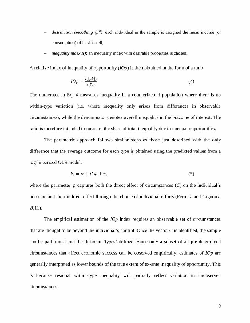
distribution smoothing {μin}: each individual in the sample is assigned the mean income (or
consumption) of her/his cell;
inequality index I(): an inequality index with desirable properties is chosen.
A relative index of inequality of opportunity (IOp) is then obtained in the form of a ratio
{
}
(4)
The numerator in Eq. 4 measures inequality in a counterfactual population where there is no
within-type variation (i.e. where inequality only arises from differences in observable
circumstances), while the denominator denotes overall inequality in the outcome of interest. The
ratio is therefore intended to measure the share of total inequality due to unequal opportunities.
The parametric approach follows similar steps as those just described with the only
difference that the average outcome for each type is obtained using the predicted values from a
log-linearized OLS model:
(5)
where the parameter captures both the direct effect of circumstances (C) on the individual’s
outcome and their indirect effect through the choice of individual efforts (Ferreira and Gignoux,
2011).
The empirical estimation of the IOp index requires an observable set of circumstances
that are thought to be beyond the individual’s control. Once the vector C is identified, the sample
can be partitioned and the different ‘types’ defined. Since only a subset of all pre-determined
circumstances that affect economic success can be observed empirically, estimates of IOp are
generally interpreted as lower bounds of the true extent of ex-ante inequality of opportunity. This
is because residual within-type inequality will partially reflect variation in unobserved
circumstances.

10
2.3 The relationship between IGE and IOp
Brunori et al. (2013) provide a review of ex-ante measures of inequality of opportunity for 41
countries. Among other results, they show evidence of a positive correlation between the index
of inequality of opportunity (IOp) and the intergenerational elasticity (IGE) across countries.9 In
fact, the IOp and the IGE can be shown to have a simple statistical link. To see this, consider the
parametric IOp when the variance is used as the inequality measure I():
(6)
which is just the R2 from the OLS regression of Eq. 5. If we were to use parental earnings as the
only circumstance variable, Eq. 5 would reduce to Eq. 1 and the R2 from this regression would
estimate the relative index of inequality of opportunity, which can be expressed as
. (7)
In this particular case, the IOp is related to the IGE (as estimated by ) and to changes in
inequality across generations (as denoted by the ratio of variances). As a special case, when
inequality is of similar magnitude in the two generations then .
The statistical link is somewhat different when the IGE is estimated by TSTSLS. If we
rename (the vector used to predict parental earnings in the first-stage regression) to , the
intergenerational equation (Eq. 3) can be rewritten as
(8)
and the resulting IOp index will be
9 For South Africa, the authors quote the estimates reported in a previous version of the present paper (presented at
the 2nd World Bank Conference on Equity, June 2012). The reported estimates are slightly different than the ones
shown below, which make use of additional data from the third wave of NIDS and are based on a narrower income
defintion.

11
(9)
which is the R2 from Eq. 8. This expression provides an insightful reformulation of the IOp
index: for a given level of earnings inequality in the current generation, , the extent of
inequality of opportunity will depend on the level of between-type inequality in the previous
generation, , and on the degree of intergenerational earnings transmission, . The
larger the difference in parental earnings across ‘types’ defined on observable circumstances, and
the larger the earnings transmission across generations, the higher the inequality of opportunity.
3. Data and Sample Selection
The empirical analysis is based on the National Income Dynamics Study (NIDS), the first
national longitudinal study in South Africa. Wave 1 of NIDS was collected in 2008 and consisted
of a nationally representative sample of approximately 7,300 households. Waves 2 and 3 were
conducted in 2010 and 2012, respectively, attempting to re-interview the same households that
were visited in 2008. Those that had moved from their original households were tracked if their
movements were within the borders of the country. NIDS used a combination of household and
individual level questionnaires to obtain information on a wide selection of human capital
variables, labour force experiences and demographic characteristics (see De Villiers et al., 2013;
for details). The present study mainly uses information from the adult questionnaire, which
includes the wages and other incomes of the adults in the household, as well as their education
level and employment status. All adults were asked to complete a section on parental
background. Key socio-economic information on non-resident and deceased parents is available
from this retrospective section, in addition to information on co-residing parents available from
other parts of the questionnaire. In the empirical analysis that follows, observations from the all
12
three waves of NIDS currently available (2008, 2010 and 2012) are pooled. A respondent who
has valid information in more than one wave is counted as a single observation and the average
value of pertinent time-variant variables is computed.
As explained in Section 2.1, estimating the intergenerational elasticity in South Africa
requires auxiliary information on earnings and socio-demographic characteristics for a sample of
‘pseudo’ parents. That is, an earlier sample representative of the national population is needed to
estimate the first-stage regression model. The Project for Statistics on Living Standards and
Development (PSLSD) that was conducted in 1993 can serve this purpose. The PSLSD was the
first nationally representative household survey conducted in South Africa. The dataset contains
a variety of socio-demographic variables as well as detailed information on income sources.
Under the apartheid regime, a large proportion of the population was excluded from official
statistics. It was not until the PSLSD that credible data on the entire population was collected.10
3.1 Analytical Sample
The empirical analysis focuses on males only. This is in line with a number of previous studies
of intergenerational earnings mobility (especially in the developing world) that prefer to abstract
from gender differences in labour force participation. The sample is restricted to men between 20
and 44 years of age, which yields a good sample size while keeping a reasonable overlap
between the birth cohort of actual fathers and that of the adult males used in the first-stage
regression.11
10
The PSLSD has a similar design to the Living Standards Measurement Surveys (LSMS) conducted by the World
Bank. Being the first nationally representative dataset for South Africa, it has been extensively used in the past 20
years (see, amongst others, Case and Deaton, 1998; Duflo 2003; Bertrand et al., 2003). For more information, see
PSLSD (1994). 11
The mean age of actual fathers in 1993 was 46.5 compared to 44.9 of pseudo-fathers.

13
The income variable used in this paper is the monthly aggregated gross employment
earnings. It includes wages, salary bonuses, shares of profit, income from agricultural activities,
casual and self-employment income.12
Individuals who report zero earnings in all survey waves
are excluded from the main analytical sample. This is an important restriction in a country like
South Africa, where a large proportion of the population is chronically unemployed. While other
measures of socioeconomic status (e.g. educational attainments or household expenditures)
would result in a higher coverage of the population, the focus of the present paper is on the
inherited determinants of earnings. Different metrics of social status result in conceptually and
empirically distinct indices of mobility and inequality. The focus on earnings allows a direct
comparison of the paper’s results to the large international evidence on earnings inequality and
mobility. Furthermore, earnings differentials have been shown to be a key feature of South
Africa’s high socio-economic inequality (Leibbrandt et al., 2010).
The estimation procedure also requires non-missing information on fathers’
socioeconomic status. About 24% of men with positive earnings do not report their father’s
education. This may be partially related to high rates of father absence in South Africa (Posel
and Devey, 2006), which might particularly affect low-income respondents. To check the
sensitivity of the results to this sample restriction, Section 4.1 replicates the main estimation
using recall information on mothers as well as fathers.
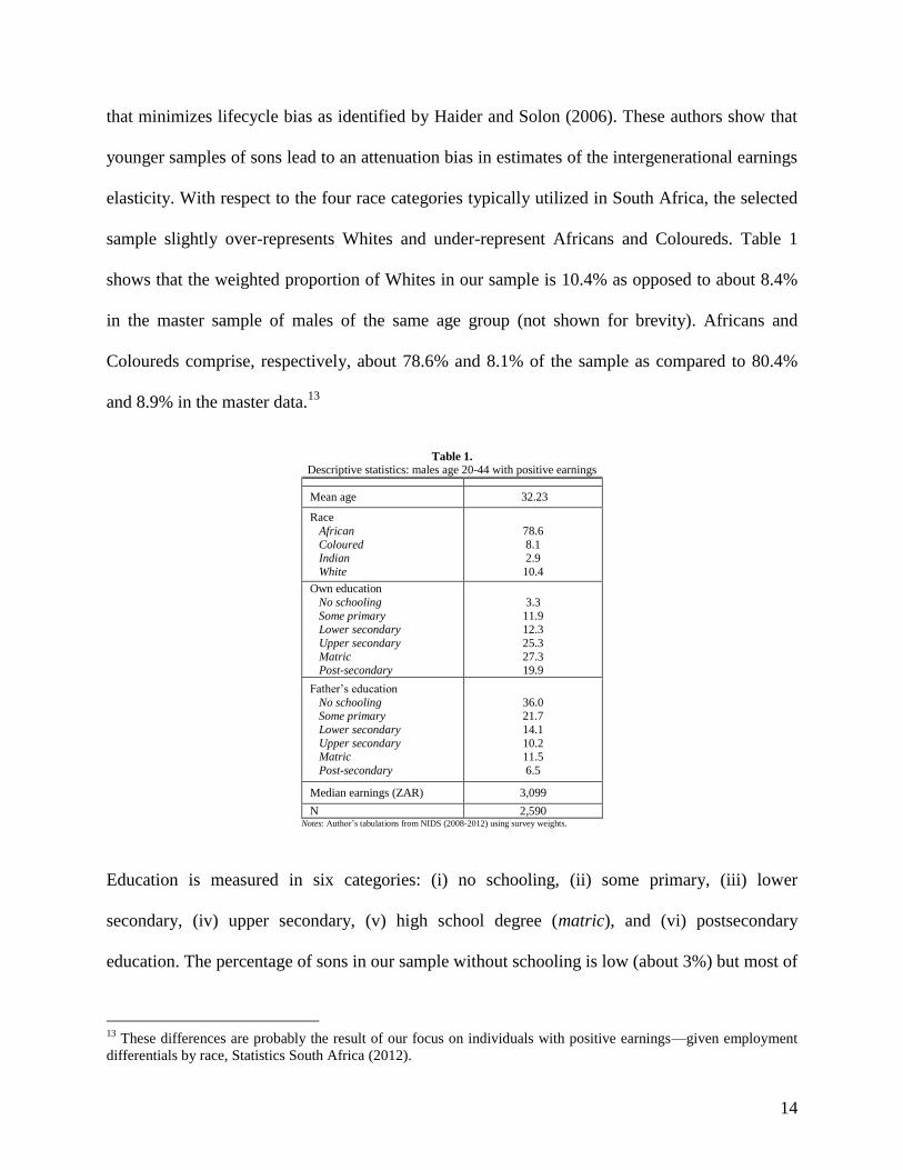
Table 1 reports some descriptive statistics for the analytical sample, which consists of
2,590 observations. As a result of the age restriction, the sample is relatively young, with a mean
age at just above 32. This implies that sons’ earnings are observed at the lower end of the range
12
This definition is narrower than total market income, which is defined as before-tax income from all market
sources (including rents and interests from investments). Previous studies have found evidence of higher
intergenerational persistence and more inequality of opportunity for broader income concepts (Corak and Heisz,
1999; Mazumder, 2005; Brunori et al., 2013).
14
that minimizes lifecycle bias as identified by Haider and Solon (2006). These authors show that
younger samples of sons lead to an attenuation bias in estimates of the intergenerational earnings
elasticity. With respect to the four race categories typically utilized in South Africa, the selected
sample slightly over-represents Whites and under-represent Africans and Coloureds. Table 1
shows that the weighted proportion of Whites in our sample is 10.4% as opposed to about 8.4%
in the master sample of males of the same age group (not shown for brevity). Africans and
Coloureds comprise, respectively, about 78.6% and 8.1% of the sample as compared to 80.4%
and 8.9% in the master data.13
Table 1.
Descriptive statistics: males age 20-44 with positive earnings
Mean age 32.23
Race
African
Coloured Indian
White
78.6
8.1 2.9
10.4
Own education
No schooling
Some primary Lower secondary
Upper secondary
Matric Post-secondary
3.3
11.9
12.3
25.3
27.3 19.9
Father’s education
No schooling Some primary
Lower secondary
Upper secondary Matric
Post-secondary
36.0 21.7
14.1
10.2 11.5
6.5
Median earnings (ZAR) 3,099
N 2,590 Notes: Author’s tabulations from NIDS (2008-2012) using survey weights.
Education is measured in six categories: (i) no schooling, (ii) some primary, (iii) lower
secondary, (iv) upper secondary, (v) high school degree (matric), and (vi) postsecondary
education. The percentage of sons in our sample without schooling is low (about 3%) but most of
13
These differences are probably the result of our focus on individuals with positive earnings—given employment
differentials by race, Statistics South Africa (2012).

15
them do not complete secondary school (matric). On the other hand, the majority of fathers have
little or no schooling (21.7% have some primary education while 36% have no education). The
significantly higher education levels of sons compared to their fathers are consistent with the
documented increase in educational attainments after the end of Apartheid (Leibbrandt et al.,
2010).14
Finally, Table 1 shows that median earnings in our sample are estimated at about 3,100
South African Rands (deflated to the year 2012).
4. Empirical results
4.1. Intergenerational earnings regression
Table 2 shows the estimates of the intergenerational earnings elasticity in South Africa. The
values shown are based on the estimation procedure outlined in section 2.1 (TSTSLS) under four
different specifications. First-stage regression coefficients of parents’ earnings are shown in
Appendix Table A1.15
The first specification—model (1)—uses only father’s education as the
predictor of his earnings. Model (2) adds father’s occupation in the first-stage regression.
Unfortunately, the detail of occupational information in the PSLSD does not match with the
categories reported in the NIDS. In order to achieve comparability between the two surveys,
occupational categories are aggregated into six larger groups: (i) elementary occupations; (ii)
clerks/service workers, (iii) craft/trade workers; (iv) agriculture/fishery workers; (v)
operators/semi-skilled workers; and (vi) professional/technical occupations/managers. While
these occupational groups partially reflect skill differentials in the South African labour market,
14
Also, to the extent that fathers with many children are overrepresented in the sample of sons, some of this
difference can be ascribed to differential childbearing by socioeconomic status. This is observed in most
intergenerational studies. 15
The PSLSD sample of pseudo-fathers consists of males 35-59 years of age with positive earnings and non-missing
information on the variables used to predict earnings. Age-adjusted earnings are used in both stages of the model to
control for age-earnings profiles.

16
they are fairly broad and display significant within-group variation in education and earnings.
For this reason, father’s occupation is best used in conjunction with other variables. Model (3)
combines father’s education with the province where the son was residing in 1994. The latter is
used as a proxy for paternal province of residence, which is not reported in the retrospective
section of the questionnaire. Finally, model (4) uses all three first-stage variables to predict
fathers’ earnings.16
Table 2.
Intergenerational earnings elasticity
First-stage variables
(1) (2) (3) (4)
Education Education &
Occupation
Education &
Province
Education &
Occupation &
Province
0.605
(0.062)
0.570
(0.091)
0.624
(0.060)
0.672
(0.079)
2,590 1,444 2,200 1,241
Notes: Author’s estimation from NIDS (2008-2012) and PSLSD (1993). Bootstrap standard errors in parentheses.
In light of the coefficients reported in Table 2, intergenerational earnings persistence in
South Africa appears to be high and significant. In all cases, bootstrapped standard errors are
reported in parentheses, to correct for the use of generated regressors.17
The estimate of β ranges
from 0.57 to 0.67 depending on the variables used to predict fathers’ earnings. Although there is
some variation in the estimates across alternative specifications of the first-stage model, the
results are consistently high and indicative that about three-fifths of the earnings advantage of
16
Different model specifications result in estimation samples of varying size. In particular, models requiring non-
missing information on father’s occupation have significantly fewer observations. Despite this variation, however,
the coefficients in Table 2 reveal a consistent picture of intergenerational earnings persistence in South Africa. 17
First, a bootstrap first-stage sample of fathers is drawn, from which the parameters used to generate predicted
earnings are estimated. Then a bootstrap sample of sons is drawn for the second-stage regression. After repeating
this process 500 times, the bootstrap standard error is estimated by the standard deviation of the distribution of the
bootstrap estimates.

17
South African fathers is passed on to their sons. These values are similar in magnitude to those
found for Brazil, China, and Chile using the same estimation technique (Ferreira and Veloso,
2006; Dunn, 2007; Gong et al., 2012; Nunez and Miranda, 2010). Overall, the estimated
coefficients for South Africa corroborate the hypothesis of a negative relationship between cross-
sectional inequality and intergenerational mobility.
As discussed in Section 2.1, the studies that have used the TSTSLS estimator
acknowledge the possibility that at least some of the first-stage predictors can have a direct effect
on the sons’ earnings, with a resulting upward bias in the estimated elasticity. Although this
possibility also applies to the estimates presented here, existing studies have shown that this bias
need not be large (Bjorklund and Jantti, 1997; Corak an Heisz, 1999). Furthermore, the relatively
young age of the sample of sons (and the use of earnings instead of total market income) would,
if anything, result in more conservative estimates of the true intergenerational elasticity (Haider
and Solon 2006; Piraino, 2007). Finally, Table A2 in the Appendix tests the sensitivity of the
estimated coefficients to the inclusion of a significant number of observations with missing
information on their fathers. Specifically, Table A2 replicates the estimation in Table 2 using
maternal characteristics in the first-stage regression for those individuals who do not report
father’s background. The results are remarkably consistent. Although these estimates still require
non-missing information on at least one parent, the minor change in the coefficients from a larger
sample is reassuring.
4.2. Inequality of opportunity index
The estimates of the index of inequality of opportunity (IOp) for South Africa are shown in
Table 3. For international comparability, Table 3 provides IOp estimates using the mean

18
logarithmic deviation (Theil-L index) as the inequality measure in the ratio of Eq. 4.18
As
explained above, the measurement of inequality of opportunity requires partitioning the sample
into a discrete number of ‘types’ by observable circumstances. Table 3 presents the results of the
estimation of Eq. 4 using both the parametric and non-parametric approach for five different
partitions of the sample. The first four partitions are based on the same inherited circumstances
that were used above to estimate the intergenerational elasticity. The fifth partition (bottom row)
shows the IOp when race is included as a circumstance along with father’s education. Race is
without doubt a pre-determined circumstance and it has an obvious relevance in the South
African context.19
Table 3 shows that the estimated IOp in South Africa ranges from 0.155 to 0.232.
Combining more circumstances in the definition of ‘types’ leads to higher IOp values. Also, the
inclusion of race seems to have a noticeable impact on the share of inequality of opportunity
(row 5) even if added only to father’s education. The parametric estimates are generally lower
than the non-parametric ones, although somewhat similar in magnitude. This is consistent with
Ferreira and Gignoux (2011) who analyse Latin American data and show that the parametric
method generally yields more conservative estimates of IOp. Overall, the values reported in
Table 3 show that more than a fifth of total earnings inequality for South African males is
explained by a parsimonious set of inherited circumstances. A comparison of these results to
other countries for which estimates are available (see review in Brunori et al. 2013) reveals that
South Africa is at the upper end of the international distribution of opportunity inequality. This is
particularly true if one considers that the estimates reported in Table 3 are based on a very small
18
Ferreira and Gignoux (2011) and Checchi and Peragine (2010) provide a description of desirable properties that
justify using the mean logarithmic deviation. 19
Race was not used to predict fathers’ earnings in the previous section because of the virtually perfect correlation
between fathers and sons in this variable As a consequence, it would have entered the sons’s equation directly and
independently of the first-stage model.

19
number of observable circumstances and on a more homogenous sample (i.e. working males)
than the overall population.
Table 3.
Index of Inequality of Opportunity.
Non-parametric Parametric
Circumstances
1. Father’s education 0.176
(0.031)
0.155
(0.033)
2. Father’s education & occupation 0.212
(0.032)
0.164
(0.042)
3. Father’s education & province 0.230
(0.032)
0.187
(0.034)
4. Father’s education & occupation & province ___
0.224
(0.044)
5. Father’s education & own race 0.232
(0.031)
0.230
(0.051)
Notes: Author’s estimation from NIDS (2008-2012). Bootstrap standard errors in parentheses.
In the non-parametric analysis, which relies on mean outcomes for each type, it is
important to avoid the occurrence of types consisting of very few observations. Appendix Table
A3 reports the maximum number of types, the mean cell size, and the proportion of types with
fewer than five observations for each partition of the sample. For the specification that combines
three circumstance variables (father’s education, occupation and province), the relatively small
sample size leads to a high incidence of cells with fewer than five observations. For this reason,
the non-parametric estimate for the partition in row 4 of Table 3 is not reported. The other
partitions have a significantly lower proportion of small cells and a high average number of
observations per type (Table A3). Moreover, the estimated values in Table 3 (both parametric
and non-parametric) are not sensitive to the exclusion of types with less than five observations.20
20
The results from this robustness check are not shown for brevity. The only notable difference is an increase in the
parametric estimate of specification 4 (Father’s education & occupation & province) to a value of 0.25.
20
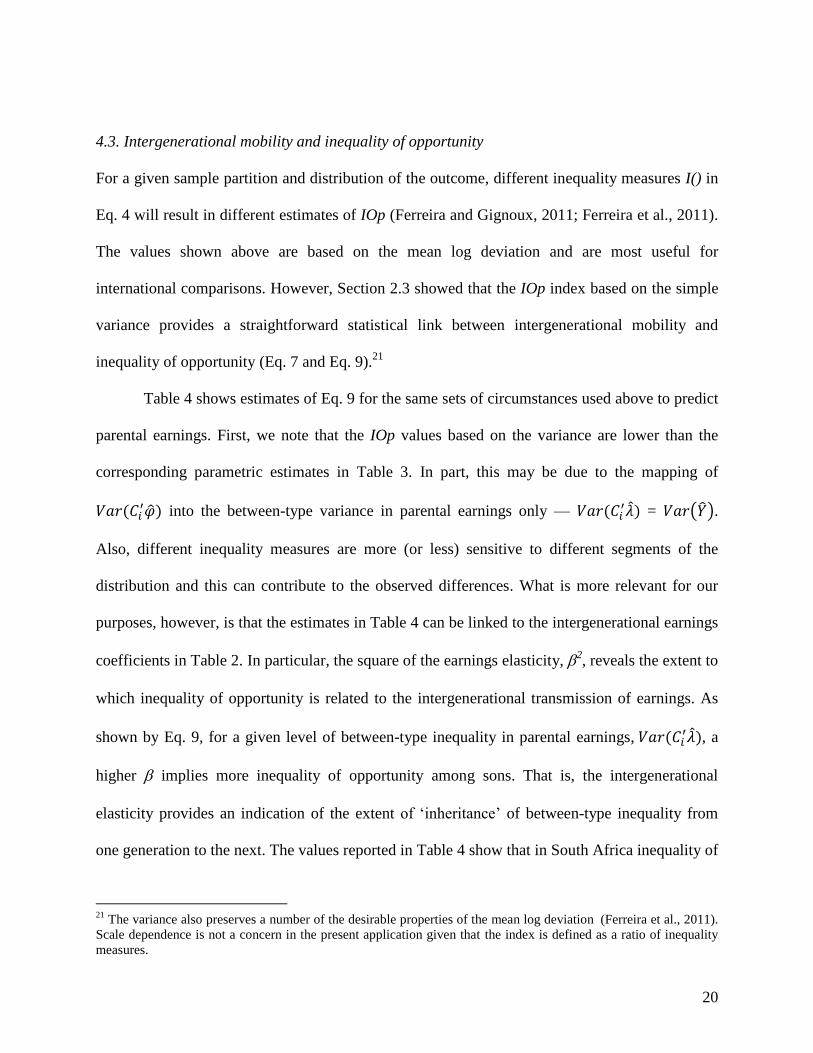
4.3. Intergenerational mobility and inequality of opportunity
For a given sample partition and distribution of the outcome, different inequality measures I() in
Eq. 4 will result in different estimates of IOp (Ferreira and Gignoux, 2011; Ferreira et al., 2011).
The values shown above are based on the mean log deviation and are most useful for
international comparisons. However, Section 2.3 showed that the IOp index based on the simple
variance provides a straightforward statistical link between intergenerational mobility and
inequality of opportunity (Eq. 7 and Eq. 9).21
Table 4 shows estimates of Eq. 9 for the same sets of circumstances used above to predict
parental earnings. First, we note that the IOp values based on the variance are lower than the
corresponding parametric estimates in Table 3. In part, this may be due to the mapping of
into the between-type variance in parental earnings only —
= ( ).
Also, different inequality measures are more (or less) sensitive to different segments of the
distribution and this can contribute to the observed differences. What is more relevant for our
purposes, however, is that the estimates in Table 4 can be linked to the intergenerational earnings
coefficients in Table 2. In particular, the square of the earnings elasticity, 2, reveals the extent to
which inequality of opportunity is related to the intergenerational transmission of earnings. As
shown by Eq. 9, for a given level of between-type inequality in parental earnings, , a
higher implies more inequality of opportunity among sons. That is, the intergenerational
elasticity provides an indication of the extent of ‘inheritance’ of between-type inequality from
one generation to the next. The values reported in Table 4 show that in South Africa inequality of
21
The variance also preserves a number of the desirable properties of the mean log deviation (Ferreira et al., 2011).
Scale dependence is not a concern in the present application given that the index is defined as a ratio of inequality
measures.
21
opportunity in earnings can to a good extent be explained by a high intergenerational earnings
transmission.22
Table 4.
Inequality of opportunity index and intergenerational elasticity.
Circumstances
1. Father’s education 0.108 0.366 0.296
2. Father’s education & occupation 0.094 0.325 0.288
3. Father’s education & Province 0.127 0.390 0.326
4. Father’s education & Occupation
& Province 0.137 0.452 0.303
Notes: Author’s estimation from NIDS (2008-2012).
5. Conclusions
A large international literature on the transmission of economic advantage across generations has
developed over the past two decades. Parent-offspring correlations in economic status quantify
the persistence of inequality from one generation to the next, and are sometimes interpreted as
measures of societies’ failure to provide equality of opportunities. A related but distinct literature
exists where the definition and direct measurement of inequality of opportunity is the main
focus. This paper combines elements from both these literatures and offers novel empirical
evidence based on South African data.
Accumulating international evidence on intergenerational mobility and inequality of
opportunity is important for a better understanding of the mechanisms underlying long-term
22
Keeping constant, a 1% decrease in would result approximately in a 2% reduction of the IOp index.
For example, a decrease in the of specification 4 from 0.672 to 0.572 (a 15% change) would decrease the IOp
index from 0.137 to 0.099 (a 28% decrease). Note however, that this type of assessment should only be seen as a
descriptive simulation, not as an analysis of causal channels.

22
persistence of inequality. Cross-national comparisons can point to a variety of institutional
factors that are related to the reproduction of inequality across generations. From this
perspective, South Africa certainly represents an interesting case to add to the international
evidence. It is a country characterized by high and persistent levels of cross-sectional inequality
(Leibbrandt et al., 2010) and it has a peculiar (and tragic) history of systematic racial
discrimination against the majority of its population.
The paper’s results indicate that inherited circumstances explain a significant fraction of
South Africa’s earnings inequality. The inequality of opportunity index is high in view of the
limited set of circumstances included in the analysis. The paper also shows that this finding can
be partially explained by high levels of intergenerational transmission of earnings. Taking into
account the possible biases arising from the data and the procedure adopted, South Africa
appears to have similar low levels of intergenerational mobility as other high-inequality
emerging economies (e.g. Brazil, Chile, and China). The results offered here can be replicated in
other countries where similar datasets are available. This can contribute to the debates around
self-determination and the appropriate role of government in leveling the economic playing field,
especially for the less studied developing world.

23
REFERENCES
Bertrand, M., Mullainathan, S. and Miller, D. (2003). ‘Public policy and extended families: evidence from
pensions in South Africa’. The World Bank Economic Review, 17(1): 27–50.
Björklund, A. and Jäntti, M. (1997). Intergenerational income mobility in Sweden compared to the United
States.” American Economic Review, 87(4): 1009–1018.
Björklund, A. and Jäntti, M. (2010). “Intergenerational income mobility and the role of family
background.” In Wiemer Salverda, Brian Nolan, and Tim Smeeding (eds). Handbook of Economic
Inequality. Oxford: Oxford University Press.
Black S.E. and Devereux P.J. (2011). “Recent developments in intergenerational mobility.”
In:Ashenfelter, O., Card, D. (Eds.), Handbook of Labor Economics. North-Holland:Amsterdam,
1487–1541.
Brunori P., Ferreira F. and Peragine V. (2013). “Inequality of opportunity, income inequality and
economic mobility: some international comparisons.” World Bank Policy Research Working Paper.
Case, A. and Deaton A. (1998). ‘Large cash transfers to the elderly in South Africa’. The Economic
Journal. 108(450): 1330–1361.
Checchi, D. and Peragine, V. (2010). Inequality of opportunity in Italy. Journal of Economic Inequality,
8(4): 429–50.
Corak, M. (2013). "Income inequality, equality of opportunity, and intergenerational mobility", Journal of
Economic Perspectives, 27(3): 79-102.
Corak, M. and Heisz, A. (1999). “The intergenerational income mobility of Canadian men.” Journal of
Human Resources, 34: 504–33.
De Villiers, L., Brown, M., Woolard, I., Daniels, R.C., and Leibbrandt, M. (2013). "National Income
Dynamics Study Wave 3 user manual", Cape Town: Southern Africa Labour and Development
Research Unit.
24
Duflo, E. (2003). ‘Grandmothers and granddaughters: old age pensions and intrahousehold allocation in
South Africa’. The World Bank Economic Review, 17(1): 1-25.
Dunn, C, E. (2007). “The intergenerational transmission of lifetime earnings: evidence from Brazil,” The
B.E. Journal of Economic Analysis & Policy: Vol. 7: Iss. 2 (Contributions), Article 2.
Ferreira, F. H. G. and Gignoux, J. (2011). The measurement of inequality of opportunity: theory and
application to Latin America. Review of Income and Wealth, 57(4): 622–57
Ferreira, F. H. G, J. Gignoux and Aran, M. (2011): “Measuring inequality of opportunity with imperfect
data: the case of Turkey”, Journal of Economic Inequality, 9(4): 651-680
Ferreira, S. and Veloso, F. (2006). "Intergenerational mobility of wages in Brazil." Brazilian Review of
Econometrics, 26(2): 181-211.
Fleurbaey M. and Peragine, V. (2013). “Ex ante versus ex post equality of opportunity”, Economica,
80(317): 118–130.
Gong, H., Leigh, A. and Meng, X. (2012). “Intergenerational income mobility in urban China.” Review of
Income and Wealth. 58(3): 397–592
Grawe, N. (2004). “Intergenerational mobility for whom? The experience of high- and low-earning sons
in international perspective.” In Generational Income Mobility in North America and Europe, edited
by Miles Corak, 58–89. Cambridge: Cambridge University Press.
Grawe, N. (2006). “The extent of lifecycle bias in estimates of intergenerational earnings persistence.”
Labour Economics, 13(5): 551-570.
Haider, S. and Solon, G. (2006) "Life-cycle variation in the association between current and lifetime
earnings." American Economic Review, 96(4): 1308-1320.
Hertz, T. (2001). “Education, inequality and economic mobility in South Africa,” PhD Dissertation,
University of Massachusetts.
Hertz, T., Jayasundera, T., Piraino, P., Selcuk, S., Smith, N. and Verashchagina, A. (2007). “The
inheritance of educational inequality: international comparisons and fifty-year trends.” The B.E.
Journal of Economic Analysis & Policy: Vol. 7: Iss. 2 (Advances), Article 10.

25
Inoue, A. and Solon, G. (2010). “Two-sample instrumental variables estimators.” The Review of
Economics and Statistics, 92(3): 557–561.
Jencks, C. and Tach, L. (2006). “Would equal opportunity mean more mobility?” in Mobility and
Inequality: Frontiers of Research in Sociology and Economics, edited by Stephen L. Morgan, David
B. Grusky and Gary S. Fields. Stanford: Stanford University Press.
Keswell, M., Girdwood, S. and Leibbrandt, M. (2013). “Educational inheritance and the distribution of
occupations: evidence from South Africa. Review of Income and Wealth. 59: S111–S137
Kruger, A. B. (2012). “Six challenges for the statistical community”.
http://www.whitehouse.gov/sites/default/files/six_challenges_for_the_statistical_community.pdf.
Leibbrandt, M., Woolard, I., Finn, A. and Argent, J. (2010). Trends in South African income distribution
and poverty since the fall of Apartheid. OECD Social, Employment and Migration Working Papers,
No. 101, OECD Publishing, OECD.
Mazumder, B. (2005). “Fortunate sons: new estimates of intergenerational mobility in the U.S. using
social security earnings data.” Review of Economics and Statistics, 87(2): 235-55.
Nunez, J. I. and Miranda, L. (2010).” Intergenerational income mobility in a less-developed, high-
inequality context: the case of Chile.” The B.E. Journal of Economic Analysis & Policy. 10(1)
(Contributions).
Piraino, P. (2007). Comparable estimates of intergenerational income mobility in Italy,” The B.E. Journal
of Economic Analysis & Policy. 7(2) (Contributions), Article 1.
Posel, D. and Devey, R. (2006). The demographics of fatherhood in South Africa: An analysis of survey
data, 1993-2002. In L. Richter & R. Morrell (Eds.), Baba: Men and fatherhood in South Africa (pp.
38-52). Cape Town: HSRC Press.
PSLSD. (1994). “Project for statistics on living standards and development: South Africans rich and poor:
baseline household statistics,” South African Labour and Development Research Unit, University of
Cape Town, South Africa.

26
Roemer, J.E. (1993). A pragmatic theory of responsibility for the egalitarian planner. Philosophy and
Public Affairs, 22(2): 146–66.
———(1998). Equality of opportunity, Harvard University Press, Cambridge.
———(2004). “Equal opportunity and intergenerational mobility: going beyond intergenerational income
transition matrices.” In Miles Corak (editor). Generational Income Mobility in North America and
Europe. Cambridge: Cambridge University Press.
Solon, G. (1992). “Intergenerational income mobility in the United States.” American Economic Review,
vol. 82(3): 393–408.
—— (1999). “Intergenerational mobility in the labor market.” In (D. Card and O. Ashenfelter, eds.),
Handbook of Labor Economics, Vol. 3: 1761–1800 Amsterdam: North-Holland.
—— (2002). “Cross-country differences in intergenerational earnings mobility.” Journal of Economic
Perspectives, 16(3): 59–66.
Statistics South Africa. (2012). Census 2011 Statistical release. Pretoria.
van de Gaer, D. (1993). Equality of opportunity and investment in human capital, PhD Dissertation,
Catholic University of Louvain, 1993.

27
APPENDIX
Table A1.
First-stage regressions on PSLSD data from 1993: males 30-59 years old.
First-stage models
(1) (2) (3) (4)
Education
some primary .351
(.099)
.245
(.090)
.314
(.098)
.242
(.088)
lower secondary .783
(.115)
.579
(.108)
.671
(.118)
.529
(.110)
upper secondary
incomplete
1.30
(.105)
.888
(.110)
1.19
(.108)
.863
(.109)
matric 1.97
(.117)
1.39
(.125)
1.87
(.121)
1.37
(.126)
postsecondary 2.27
(.117)
1.36
(.154)
2.11
(.120)
1.31
(.154)
Occupation
professional/manager 1.83
(.159)
1.81
(.166)
operator/semi-skilled 1.25
(.126)
1.30
(.132)
craft/trade
1.19
(.157)
1.15
(.161)
clerk/sales 1.00
(.124)
.983
(.131)
elementary occupations .685
(.117)
.719
(.120)
Province dummies no no yes yes
R2 .35 .44 .37 .46
N 1,355 1,292 1,355 1,292 Notes: Author’s estimations based on PSLSD. Reference categories are ‘no education’, and ‘agriculture/fishery’.
Table A2.
Intergenerational earnings elasticity using information on mothers
First-stage variables
(1) (2) (3) (4)
Education Education &
Occupation
Education &
Province
Education &
Occupation &
Province
0.574
(0.054)
0.505
(0.070)
0.595
(0.050)
0.609
(0.059)
3,121 1,891 2,651 1,614
Notes: Author’s estimation from NIDS (2008-2012) and PSLSD (1993). Bootstrap standard errors in parentheses.

28
Table A3.
Sample Partition
1. Father’s
education
2. Father’s
education &
occupation
3. Father’s
education &
province
4. Father’s
education &
occupation
& province
5. Father’s
education &
own race
N 2,590 1,444 2,200 1,241 2,590
Maximum number of
types 6 36 54 324 24
Number of types
observed 6 36 54 259 24
Mean number of
observations per type 680.9 81.1 79.8 9.4 501.2
Proportion of types with
fewer than 5 obs. 0 0.08 0.02 0.66 0.16
Notes: Authors calculations from NIDS (2008-2012).

The Southern Africa Labour and Development Research Unit (SALDRU) conducts research directed at improving the well-being of South Africa’s poor. It was established in 1975. Over the next two decades the unit’s research played a central role in documenting the human costs of apartheid. Key projects from this period included the Farm Labour Conference (1976), the Economics of Health Care Conference (1978), and the Second Carnegie Enquiry into Poverty and Development in South Africa (1983-86). At the urging of the African National Congress, from 1992-1994 SALDRU and the World Bank coordinated the Project for Statistics on Living Standards and Development (PSLSD). This project provide baseline data for the implementation of post-apartheid socio-economic policies through South Africa’s fi rst non-racial national sample survey. In the post-apartheid period, SALDRU has continued to gather data and conduct research directed at informing and assessing anti-poverty policy. In line with its historical contribution, SALDRU’s researchers continue to conduct research detailing changing patterns of well-being in South Africa and assessing the impact of government policy on the poor. Current research work falls into the following research themes: post-apartheid poverty; employment and migration dynamics; family support structures in an era of rapid social change; public works and public infrastructure programmes, fi nancial strategies of the poor; common property resources and the poor. Key survey projects include the Langeberg Integrated Family Survey (1999), the Khayelitsha/Mitchell’s Plain Survey (2000), the ongoing Cape Area Panel Study (2001-) and the Financial Diaries Project.
www.saldru.uct.ac.za
Level 3, School of Economics Building, Middle Campus, University of Cape Town
Private Bag, Rondebosch 7701, Cape Town, South Africa
Tel: +27 (0)21 650 5696
Fax: +27 (0) 21 650 5797
Web: www.saldru.uct.ac.za
southern africa labour and development research unit