Interface Dynamics in the Transcritical Flow of Liquid

Fuels into High-Pressure Combustors

Lluıs Jofre∗ and Javier Urzay†

Center for Turbulence Research, Stanford University, Stanford, CA 94305, USA

Rocket engines and new generations of high-pressure gas turbines and diesel enginesoftentimes involve atomization, vaporization and combustion of propellants injected atsubcritical temperature into an environment at a pressure larger than that of the corre-sponding critical points of the individual components of the mixture. This class of tra-jectories in the thermodynamic space have been referred to as transcritical. As a result,relatively sharp interfaces may persist in pressure and temperature conditions where theywere not expected to exist. This is particularly relevant in hydrocarbon-fueled mixturesthat display a critical-point elevation property by which the two-phase region extends upto pressures much larger than the critical pressures of the individual components. As aconsequence, linear thermodynamic trajectories emulating typical injection conditions fre-quently pass through the two-phase region, thus indicating that the mixture may becomeseparated there into liquid and vapor phases by an interface. In this study, a set of mod-ifications to the Navier-Stokes equations for multi-component flows is proposed based ondiffuse-interface theory in order to treat the emergent and vanishing interfaces in the sameflow field. This requires appropriate alterations of the stress tensor and diffusive fluxesof heat and species. The resulting transport formulation is particularized for binary mix-tures, as well as collapsed to single-component gradient theory for stationary quasi-planarvapor-liquid interfaces.

Nomenclature

a, b Equation of state coefficientsc Molar density, mol/m3

D Diffusion coefficient, m2/sE Specific total energy, J/kge Specific internal energy, J/kgF Helmholtz free energy, Jf Specific Helmholtz free energy, J/kgG Gibbs free energy, Jh Specific enthalpy, J/kgJ,J Species diffusion fluxes, kg/(s·m2)N Number of speciesn Number of molsNA Avogadro’s number, 1/molP Pressure, barq,Q Heat diffusion fluxes, J/(s·m2)qc Heat conduction flux, J/(s·m2)R0 Ideal gas constant, J/(K·mol)s Specific entropy, J/(kg·K)sprod Entropy production rate, J/(K·s·m3)T Temperature, K

t Time, sv velocity vector, m/sv Molar volume, mol/kgW Molecular weight, kg/molX Molar fractionY Mass fractionZ Compressibility factorη, ζ Shear and bulk viscosities, Pa·sκ Gradient-energy coefficient, m7/(kg·s2)λ Thermal conductivity, W/(m·K)µ Molar chemical potential, J/molρ Density, kg/m3

σ Surface-tension coefficient, N/mτ ,K Stress tensors, N/m2

ϕ Fugacity coefficient

Subscriptsc Critical pointi, j Species indexNL Non-local quantity

∗Postdoctoral Researcher. E-mail: jofre@stanford.edu†Senior Research Engineer. E-mail: jurzay@stanford.edu

1 of 14

American Institute of Aeronautics and Astronautics

Dow

nloa

ded

by S

TA

NFO

RD

UN

IVE

RSI

TY

on

Nov

embe

r 17

, 201

7 | h

ttp://

arc.

aiaa

.org

| D

OI:

10.

2514

/6.2

017-

4940

53rd AIAA/SAE/ASEE Joint Propulsion Conference

10-12 July 2017, Atlanta, GA

10.2514/6.2017-4940

Copyright © 2017 by the American Institute of Aeronautics and Astronautics, Inc.

All rights reserved.

AIAA Propulsion and Energy Forum

I. Introduction

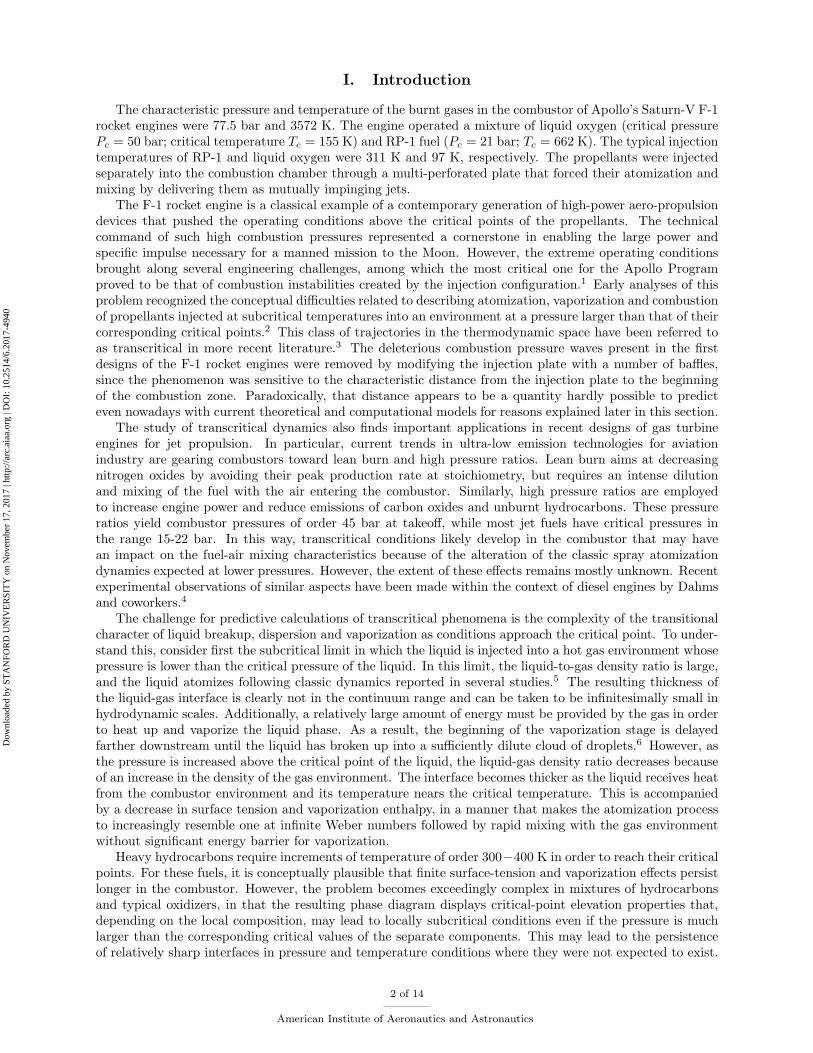
The characteristic pressure and temperature of the burnt gases in the combustor of Apollo’s Saturn-V F-1rocket engines were 77.5 bar and 3572 K. The engine operated a mixture of liquid oxygen (critical pressurePc = 50 bar; critical temperature Tc = 155 K) and RP-1 fuel (Pc = 21 bar; Tc = 662 K). The typical injectiontemperatures of RP-1 and liquid oxygen were 311 K and 97 K, respectively. The propellants were injectedseparately into the combustion chamber through a multi-perforated plate that forced their atomization andmixing by delivering them as mutually impinging jets.

The F-1 rocket engine is a classical example of a contemporary generation of high-power aero-propulsiondevices that pushed the operating conditions above the critical points of the propellants. The technicalcommand of such high combustion pressures represented a cornerstone in enabling the large power andspecific impulse necessary for a manned mission to the Moon. However, the extreme operating conditionsbrought along several engineering challenges, among which the most critical one for the Apollo Programproved to be that of combustion instabilities created by the injection configuration.1 Early analyses of thisproblem recognized the conceptual difficulties related to describing atomization, vaporization and combustionof propellants injected at subcritical temperatures into an environment at a pressure larger than that of theircorresponding critical points.2 This class of trajectories in the thermodynamic space have been referred toas transcritical in more recent literature.3 The deleterious combustion pressure waves present in the firstdesigns of the F-1 rocket engines were removed by modifying the injection plate with a number of baffles,since the phenomenon was sensitive to the characteristic distance from the injection plate to the beginningof the combustion zone. Paradoxically, that distance appears to be a quantity hardly possible to predicteven nowadays with current theoretical and computational models for reasons explained later in this section.

The study of transcritical dynamics also finds important applications in recent designs of gas turbineengines for jet propulsion. In particular, current trends in ultra-low emission technologies for aviationindustry are gearing combustors toward lean burn and high pressure ratios. Lean burn aims at decreasingnitrogen oxides by avoiding their peak production rate at stoichiometry, but requires an intense dilutionand mixing of the fuel with the air entering the combustor. Similarly, high pressure ratios are employedto increase engine power and reduce emissions of carbon oxides and unburnt hydrocarbons. These pressureratios yield combustor pressures of order 45 bar at takeoff, while most jet fuels have critical pressures inthe range 15-22 bar. In this way, transcritical conditions likely develop in the combustor that may havean impact on the fuel-air mixing characteristics because of the alteration of the classic spray atomizationdynamics expected at lower pressures. However, the extent of these effects remains mostly unknown. Recentexperimental observations of similar aspects have been made within the context of diesel engines by Dahmsand coworkers.4

The challenge for predictive calculations of transcritical phenomena is the complexity of the transitionalcharacter of liquid breakup, dispersion and vaporization as conditions approach the critical point. To under-stand this, consider first the subcritical limit in which the liquid is injected into a hot gas environment whosepressure is lower than the critical pressure of the liquid. In this limit, the liquid-to-gas density ratio is large,and the liquid atomizes following classic dynamics reported in several studies.5 The resulting thickness ofthe liquid-gas interface is clearly not in the continuum range and can be taken to be infinitesimally small inhydrodynamic scales. Additionally, a relatively large amount of energy must be provided by the gas in orderto heat up and vaporize the liquid phase. As a result, the beginning of the vaporization stage is delayedfarther downstream until the liquid has broken up into a sufficiently dilute cloud of droplets.6 However, asthe pressure is increased above the critical point of the liquid, the liquid-gas density ratio decreases becauseof an increase in the density of the gas environment. The interface becomes thicker as the liquid receives heatfrom the combustor environment and its temperature nears the critical temperature. This is accompaniedby a decrease in surface tension and vaporization enthalpy, in a manner that makes the atomization processto increasingly resemble one at infinite Weber numbers followed by rapid mixing with the gas environmentwithout significant energy barrier for vaporization.

Heavy hydrocarbons require increments of temperature of order 300−400 K in order to reach their criticalpoints. For these fuels, it is conceptually plausible that finite surface-tension and vaporization effects persistlonger in the combustor. However, the problem becomes exceedingly complex in mixtures of hydrocarbonsand typical oxidizers, in that the resulting phase diagram displays critical-point elevation properties that,depending on the local composition, may lead to locally subcritical conditions even if the pressure is muchlarger than the corresponding critical values of the separate components. This may lead to the persistenceof relatively sharp interfaces in pressure and temperature conditions where they were not expected to exist.

2 of 14

American Institute of Aeronautics and Astronautics

Dow

nloa

ded

by S

TA

NFO

RD

UN

IVE

RSI

TY

on

Nov

embe

r 17

, 201

7 | h

ttp://

arc.

aiaa

.org

| D

OI:

10.

2514

/6.2

017-

4940

Note that for single-component systems consisting of a liquid atomizing in its own vapor, the description ofthe dynamics becomes much simpler, in that there is practically no distinction between the two phases atpressures above the critical point. Accordingly, the interface disappears, and the surface tension vanishes.The single-component case, however, is not the one found in most practical applications. Additional factorsthat prevent further understanding of transcritical dynamics are the large uncertainties in high-pressurephysical properties of complex mixtures of reactants and combustion products, and the lack of quantitativeexperimental diagnostics for model validation in such extreme environments.

This work addresses basic theoretical aspects of flow transport under transcritical conditions. It isorganized as follows. In Section II, a phase diagram for a typical hydrocarbon-fueled system is describedthat illustrates the thermodynamic space of solutions at high pressures and describes critical-point elevationproperties. Section III is devoted to a derivation of a set of conservation equations that simultaneouslyconsider surface-tension effects along with relatively permeable interfaces. Lastly, conclusions are providedin Section IV . This report builds on recent analyses from Ref.7 by providing different perspectives of theformulation and additional considerations that may be of practical use in the computation of hydrocarbon-fueled transcritical flows.

II. Phase diagrams and critical-point elevation properties ofhydrocarbon-fueled mixtures

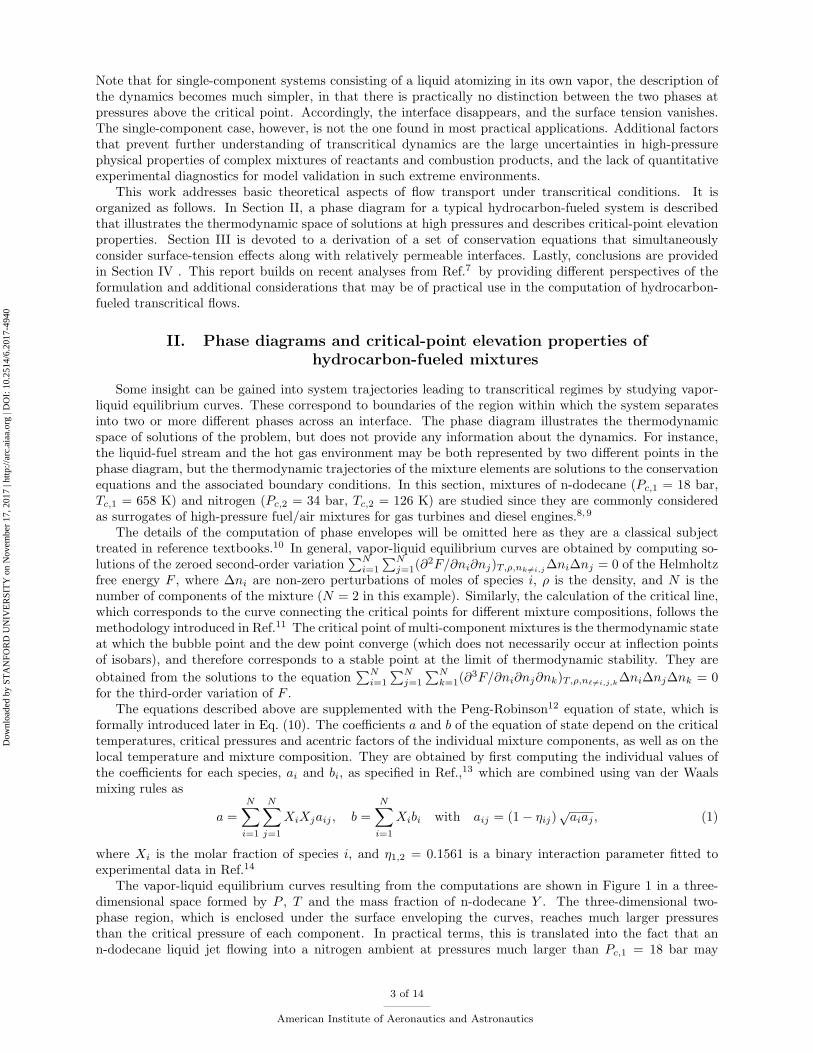
Some insight can be gained into system trajectories leading to transcritical regimes by studying vapor-liquid equilibrium curves. These correspond to boundaries of the region within which the system separatesinto two or more different phases across an interface. The phase diagram illustrates the thermodynamicspace of solutions of the problem, but does not provide any information about the dynamics. For instance,the liquid-fuel stream and the hot gas environment may be both represented by two different points in thephase diagram, but the thermodynamic trajectories of the mixture elements are solutions to the conservationequations and the associated boundary conditions. In this section, mixtures of n-dodecane (Pc,1 = 18 bar,Tc,1 = 658 K) and nitrogen (Pc,2 = 34 bar, Tc,2 = 126 K) are studied since they are commonly consideredas surrogates of high-pressure fuel/air mixtures for gas turbines and diesel engines.8,9

The details of the computation of phase envelopes will be omitted here as they are a classical subjecttreated in reference textbooks.10 In general, vapor-liquid equilibrium curves are obtained by computing so-lutions of the zeroed second-order variation

∑Ni=1

∑Nj=1(∂2F/∂ni∂nj)T,ρ,nk 6=i,j

∆ni∆nj = 0 of the Helmholtzfree energy F , where ∆ni are non-zero perturbations of moles of species i, ρ is the density, and N is thenumber of components of the mixture (N = 2 in this example). Similarly, the calculation of the critical line,which corresponds to the curve connecting the critical points for different mixture compositions, follows themethodology introduced in Ref.11 The critical point of multi-component mixtures is the thermodynamic stateat which the bubble point and the dew point converge (which does not necessarily occur at inflection pointsof isobars), and therefore corresponds to a stable point at the limit of thermodynamic stability. They areobtained from the solutions to the equation

∑Ni=1

∑Nj=1

∑Nk=1(∂3F/∂ni∂nj∂nk)T,ρ,n` 6=i,j,k

∆ni∆nj∆nk = 0for the third-order variation of F .

The equations described above are supplemented with the Peng-Robinson12 equation of state, which isformally introduced later in Eq. (10). The coefficients a and b of the equation of state depend on the criticaltemperatures, critical pressures and acentric factors of the individual mixture components, as well as on thelocal temperature and mixture composition. They are obtained by first computing the individual values ofthe coefficients for each species, ai and bi, as specified in Ref.,13 which are combined using van der Waalsmixing rules as

a =N∑i=1

N∑j=1

XiXjaij , b =N∑i=1

Xibi with aij = (1− ηij)√aiaj , (1)

where Xi is the molar fraction of species i, and η1,2 = 0.1561 is a binary interaction parameter fitted toexperimental data in Ref.14

The vapor-liquid equilibrium curves resulting from the computations are shown in Figure 1 in a three-dimensional space formed by P , T and the mass fraction of n-dodecane Y . The three-dimensional two-phase region, which is enclosed under the surface enveloping the curves, reaches much larger pressuresthan the critical pressure of each component. In practical terms, this is translated into the fact that ann-dodecane liquid jet flowing into a nitrogen ambient at pressures much larger than Pc,1 = 18 bar may

3 of 14

American Institute of Aeronautics and Astronautics

Dow

nloa

ded

by S

TA

NFO

RD

UN

IVE

RSI

TY

on

Nov

embe

r 17

, 201

7 | h

ttp://

arc.

aiaa

.org

| D

OI:

10.

2514

/6.2

017-

4940

Figure 1. Vapor-liquid equilibrium curves (solid lines) for n-dodecane/nitrogen mixtures colored by pressure, withY indicating the mass fraction of n-dodecane. Pure-substance boiling lines for nitrogen (dashed red) and n-dodecane(dashed blue) are shown, along with their corresponding critical points (squares). Experimentally measured criticalpoints are denoted by triangles.

undergo transcritical trajectories that cross the two-phase region. As a result, such flow may display remnanteffects of surface tension and atomization characteristics similar to lower pressure jets that in principle werenot expected to be observed in these thermodynamic conditions, as shown in experiments in Ref.8 Thiscritical-point elevation property is also illustrated by the divergence of the the critical line arriving to thenitrogen side, as observed in Figure 2, which indicates that the two-phase region is unbounded in pressure.Conversely, the critical line starting at the nitrogen critical point meets a liquid-liquid-gas phase-equilibriumline (indistinguishable from the nitrogen boiling line in the scales of Figure 2) at an upper critical end point.The three-phase equilibrium line continues toward lower pressures and temperatures between the boilinglines of the two pure components, thereby suggesting that the crossing of the three-phase equilibrium regionis only relevant at pressures lower than Pc,2 = 34 bar and across a very narrow range of temperatures aroundTc,2 = 126 K. The phenomena of divergence of the critical line and occurrence of three-phase equilibria aretypical in mixtures classified as class-II/type-III according to the analysis in Ref.15 This group of mixtures,to which other n-alkane/nitrogen systems also belong, is characterized by individual components with verydifferent critical temperatures.

It should be stressed that the computation of critical points in complex mixtures involves a number ofassumptions and model parameter values that find little justification on physical grounds. For instance, themixing rules (1) correspond to an ad-hoc molar weighting of the individual coefficients ai and bi, whose ex-pressions depend on calibrated interaction parameters and measured critical points of the pure substances.13

However, it is of some interest to note that the resulting divergent trend of the critical line computed from thevapor-liquid equilibrium agrees well with the values experimentally obtained in Ref.,14 as shown in Figures 1and 2.

The phase diagram facilitates the understanding of the thermodynamic trajectories involved in the in-jection of hydrocarbon fuels into high-pressure environments. As an illustration, consider the examples oflinear thermodynamic trajectories followed by mixture elements in the problem of a liquid n-dodecane jet in-jected in a nitrogen environment at 900 K, which are provided in Figure 3. Two fuel injection temperatures,corresponding to 363 K (case 1) and 563 K (case 2), are studied, along with three nitrogen-environmentpressures, namely, 50, 100, and 200 bar. The trajectories are superimposed on maximum-temperature curvesbounding the two-phase region at each pressure. Note that the trajectories resulting from integration of theconservation equations may not be generally linear.16

For all pressure values considered in case 1, the mixture elements start as compressed liquids in then-dodecane stream. As heat is supplied from the surrounding gas, the mixture elements enter the two-phaseregion where they necessarily separate into liquid and vapor phases by an interface where surface-tensionforces operate. The mixture elements eventually exit the two-phase region and change phase to a supercriticalstate while mixing with the surrounding nitrogen gas. On the other hand, in case 2, the intersection with thetwo-phase region is completely avoided for the largest pressure value considered in the nitrogen environment.

4 of 14

American Institute of Aeronautics and Astronautics

Dow

nloa

ded

by S

TA

NFO

RD

UN

IVE

RSI

TY

on

Nov

embe

r 17

, 201

7 | h

ttp://

arc.

aiaa

.org

| D

OI:

10.

2514

/6.2

017-

4940

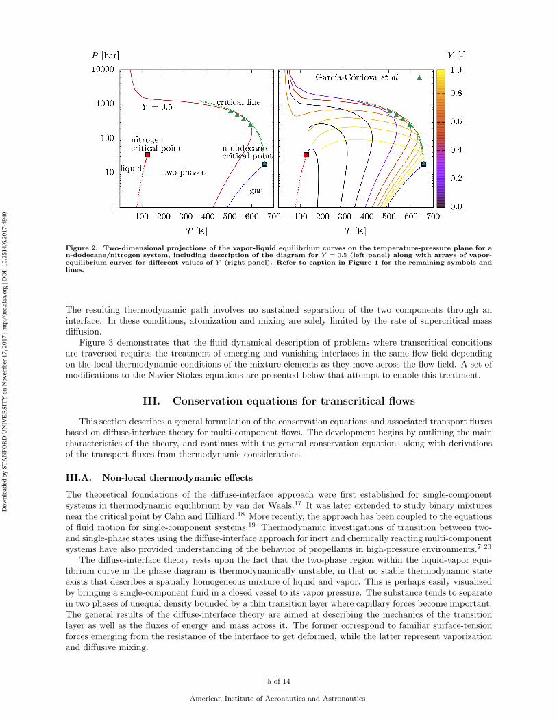
Figure 2. Two-dimensional projections of the vapor-liquid equilibrium curves on the temperature-pressure plane for an-dodecane/nitrogen system, including description of the diagram for Y = 0.5 (left panel) along with arrays of vapor-equilibrium curves for different values of Y (right panel). Refer to caption in Figure 1 for the remaining symbols andlines.

The resulting thermodynamic path involves no sustained separation of the two components through aninterface. In these conditions, atomization and mixing are solely limited by the rate of supercritical massdiffusion.

Figure 3 demonstrates that the fluid dynamical description of problems where transcritical conditionsare traversed requires the treatment of emerging and vanishing interfaces in the same flow field dependingon the local thermodynamic conditions of the mixture elements as they move across the flow field. A set ofmodifications to the Navier-Stokes equations are presented below that attempt to enable this treatment.

III. Conservation equations for transcritical flows

This section describes a general formulation of the conservation equations and associated transport fluxesbased on diffuse-interface theory for multi-component flows. The development begins by outlining the maincharacteristics of the theory, and continues with the general conservation equations along with derivationsof the transport fluxes from thermodynamic considerations.

III.A. Non-local thermodynamic effects

The theoretical foundations of the diffuse-interface approach were first established for single-componentsystems in thermodynamic equilibrium by van der Waals.17 It was later extended to study binary mixturesnear the critical point by Cahn and Hilliard.18 More recently, the approach has been coupled to the equationsof fluid motion for single-component systems.19 Thermodynamic investigations of transition between two-and single-phase states using the diffuse-interface approach for inert and chemically reacting multi-componentsystems have also provided understanding of the behavior of propellants in high-pressure environments.7,20

The diffuse-interface theory rests upon the fact that the two-phase region within the liquid-vapor equi-librium curve in the phase diagram is thermodynamically unstable, in that no stable thermodynamic stateexists that describes a spatially homogeneous mixture of liquid and vapor. This is perhaps easily visualizedby bringing a single-component fluid in a closed vessel to its vapor pressure. The substance tends to separatein two phases of unequal density bounded by a thin transition layer where capillary forces become important.The general results of the diffuse-interface theory are aimed at describing the mechanics of the transitionlayer as well as the fluxes of energy and mass across it. The former correspond to familiar surface-tensionforces emerging from the resistance of the interface to get deformed, while the latter represent vaporizationand diffusive mixing.

5 of 14

American Institute of Aeronautics and Astronautics

Dow

nloa

ded

by S

TA

NFO

RD

UN

IVE

RSI

TY

on

Nov

embe

r 17

, 201

7 | h

ttp://

arc.

aiaa

.org

| D

OI:

10.

2514

/6.2

017-

4940

Figure 3. Examples of linear thermodynamic trajectories (solid lines) superimposed on maximum-temperature curves(dashed colored lines) bounding the two-phase region of n-dodecane/nitrogen mixtures at nitrogen-environment pres-sures of 50, 100, and 200 bar. Symbols denote the thermodynamic conditions of the nitrogen environment (left-hand-sidesquare) and n-dodecane stream at 363 K (lower right-hand-side square) and 663 K (upper right-hand-side square). Thediamond symbols represent critical points at the corresponding pressure.

The description of the structure of the transition layer requires consideration of non-local thermodynamicpotentials, where the non-locality is represented by gradients of selected variables. Additional considerationsbased on the second principle of thermodynamics typically preclude non-locality to be expressed only interms of composition or density gradients (e.g., see Ref.21 for details on the mathematical justification).The analysis is facilitated when the degree of non-locality is assumed to be small, with the characteristiclength of the composition gradients being large compared to intermolecular distances, which typically limitsthe theory to situations when the interface is relatively thick compared to the molecular mean free path, asin conditions near and above the critical point. In this limit, the disturbances of the local thermodynamicstate are proportional to the square of the composition gradients in the first approximation.18 For instance,the non-local corrections to the specific values of Helmholtz free energy f , internal energy e and entropy sare

fNL = f +12ρ

N∑i=1

N∑j=1

κij∇ρi∇ρj , eNL = e+12ρ

N∑i=1

N∑j=1

κeij∇ρi∇ρj ,

sNL = s+12ρ

N∑i=1

N∑j=1

κsij∇ρi∇ρj , (2)

where ρ is the mixture density, ρi is the partial density of species i, and N is the number of species.Additionally, κij , κeij and κsij are gradient-energy coefficients, which can be computed directly as a function ofcollision parameters from kinetic-theory considerations of interactions between molecules in regions subjectedto macroscopic density gradients (e.g., see Ref.22 and Chapter 1 in Ref.23).

Since the gradient-energy coefficients κij are related to the interface thickness and surface tension, theirprecise characterization is central to the predictions of the diffuse-interface theory. However, appropriateformulations of this parameters are lacking, and most investigations utilize relations of the type κij =√κiiκjj = κji for the cross-influence coefficients i 6= j, along with empirical correlations for the individual

coefficients κii such as24

ln(

κii

aibi2/3

N8/3A

)= κ0,i + κ1,i ln

(1− T

Tc,i

)+ κ2,i

[ln(

1− T

Tc,i

)]2

(3)

6 of 14

American Institute of Aeronautics and Astronautics

Dow

nloa

ded

by S

TA

NFO

RD

UN

IVE

RSI

TY

on

Nov

embe

r 17

, 201

7 | h

ttp://

arc.

aiaa

.org

| D

OI:

10.

2514

/6.2

017-

4940

for T/Tc,i ≤ 0.95, where Tc,i is the critical temperature value, and NA is the Avogadro’s number. In Eq. (3),the correlation coefficients κ0,i, κ1,i and κ2,i are usually calibrated based on experimental measurements ofsurface tension, while the parameters ai and bi correspond to coefficients of the equation of state, as describedin Section II. Note that models such as Eq. (3) typically yield κii = 0 above the critical temperature ofthe corresponding species, as suggested by the fact that the surface tension vanishes for single-componentsystems above the critical point. For instance, in the n-dodecane/nitrogen system described in Section II,the relevant gradient-energy coefficient becomes that of the n-dodecane, κ1,1, since the temperature in theflow is larger than the critical temperature of nitrogen everywhere (i.e., κ2,2 = κ1,2 = κ2,1 = 0).

Exact expressions relating the gradient-energy coefficients κij , κeij and κsij can be easily derived bysubstituting the relations (2) into the definition of the local Helmholtz free energy, f = e − Ts, withs = −(∂f/∂T )ρ,ni

, thereby yielding

κeij = κij + T

(∂κij∂T

)ρ,nk

and κsij = −(∂κij∂T

)ρ,nk

. (4)

The consideration of non-local thermodynamic potentials, as in Eqs. (2)-(4), leads to the emergence ofinterface-related transport fluxes and mechanical stresses in the conservation equations as described below.

III.B. Conservation equations

The description of thin interfaces and their dynamics in conjunction with the outer fluid motion in a singleEulerian field requires non-trivial extensions of the Navier-Stokes conservation equations. In principle, thederivation of these modifications from molecular considerations and first principles is a difficult task dueto the lack of a clear physical understanding of the molecular structure of fluids across the critical point.In this study, a phenomenological approach is followed based on a linear augmentation of the deviatoricpart of the stress tensor, τ , and the heat and species diffusion fluxes, q and Ji, with the correspondinginterfacial transport terms K, Q and Ji derived from the diffuse-interface theory. These, as shown below,can be made to satisfy certain conditions of entropy maximization that are in accord with the second law ofthermodynamics. The resulting conservation equations for mass, momentum, species and total energy are

∂ρ

∂t+∇ · (ρv) = 0, (5)

∂ (ρv)∂t

+∇ · (ρv ⊗ v) = −∇PNL +∇ · (τ + K) , (6)

∂ (ρYi)∂t

+∇ · (ρvYi) = −∇ · (Ji + Ji) , i = 1, ..., N, (7)

∂ (ρE)∂t

+∇ · (ρvE) = −∇ · (PNLv)−∇ · (q + Q) +∇ · [(τ + K) · v] , (8)

which describe the continuum dynamics of a multi-phase, multi-component fluid of N species that moves at amass-averaged velocity v and has a local density ρ and total energy E, and which may contain thin interfacesseparating different phases. In this formulation, Yi is the mass fraction of species i, q = qc +

∑Ni=1 hiJi is

the sum of the heat conduction and the energy flux by inter-diffusion, hi is the partial specific enthalpy, andPNL a non-local thermodynamic pressure defined as

PNL = P − 12

N∑i=1

N∑j=1

κij∇ρi∇ρj . (9)

The convenience of redefining pressure as in Eq. (9), will become clear in Section III.C. In Eq. (9) the localthermodynamic pressure P can be obtained, for instance, from the cubic equation of state12

P =R0T

v − b− a

v2 + 2bv − b2, (10)

whose utilization is beneficial at the high pressures considered here. In the notation, v = W/ρ is the molarvolume, with W = (

∑i=1 Yi/Wi)−1 the mean molecular weight. The coefficients a and b, which correspond

to mixture-averaged versions of the pure-substance ones ai and bi as in Eq. (1), account for real-gas effects

7 of 14

American Institute of Aeronautics and Astronautics

Dow

nloa

ded

by S

TA

NFO

RD

UN

IVE

RSI

TY

on

Nov

embe

r 17

, 201

7 | h

ttp://

arc.

aiaa

.org

| D

OI:

10.

2514

/6.2

017-

4940

such as finite packing and increased intermolecular interactions at large densities and pressures. It should bestressed that the choice of Eq. (10) is not central to the diffuse-interface formalism insofar as it reproducesthe multivalued character of the mixture density in conditions of phase change. Note that several otherequations of state are available in the literature that have similar characteristics.25,26

Chemical conversion sources have been excluded for simplicity from Eq. (7). Gas-phase combustionreactions tend to occur far from interfaces and in regions where the local mass fraction of fuel vapor issufficiently small to warrant stoichiometric proportions. However, this approximation may not be appropriateif thermal decomposition of the liquid fuel plays an important role in modifying the interface properties.

In the species conservation equation (7), the different N components of the mixture are described bytheir corresponding mass fractions irrespectively of their phase state. Note that this is in contrast withtraditional treatments of dispersed multi-phase flows, where the gas and liquid mass fractions are describedby their corresponding conservation equations. In the diffuse-interface formulation, the phases are separatedby interfaces in thermodynamic conditions corresponding to the two-phase region. In those situations,the interfacial stress tensor K in the momentum equation (6) provides information about the dynamicalequilibrium of the separating interface, while the fluxes Q and Ji modify the transport of heat and massacross the interface accordingly. The high-pressure characteristics of the transport fluxes are described indetail in Section III.C.

A complete description of the mixture state requires specification of the analytical form of the thermo-dynamic potentials. At high pressures, increasing departures from the ideal-gas theory are observed, andconsequently, derivation of more complex expressions are necessary. A common approach to express high-pressure real-gas thermodynamic potentials is to decompose them into the sum of their ideal-gas counterparts(denoted below by the superscript 0) and departure functions that measure deviations with respect to theideal-gas behavior.28 For instance, the departure function for the molar enthalpy is

h− h0 =∫ T

T 0C0p dT +

∫ P

0

[v − T

(∂v

∂T

)P

]dP, (11)

where h0 and C0p are the ideal-gas reference molar values of enthalpy and constant-pressure heat capacity,

with T 0 = 298.15 K. Subsequently, the molar internal energy can be obtained from the enthalpy definitionas

e = h− Pv. (12)

These expressions are valid for any equation of state. Exact forms of the departure functions for multi-speciesmixtures can be found in Ref.29 for the Peng-Robinson equation of state.

Similar considerations apply for the molar chemical potential

µi =(∂G

∂ni

)T,P,nj 6=i

(13)

defined as the partial molar of the Gibbs free energy G. The corresponding decomposition is given by

µi = µ0i + R0T lnϕi, (14)

where µ0i (T, P ) is the ideal-gas counterpart. In Eq. (14), the departure function involves the dimensionless

fugacity coefficient ϕi = fi/(XiP ), which represents the ratio of the fugacity fi to the partial pressure. Inparticular, for the Peng-Robinson equation of state, the logarithm of the fugacity coefficient becomes

lnϕi =bib

(Z − 1)− ln (Z −B)− A

2√

2B

[2∑Nj=1Xiaij

a− bib

]ln

[Z +

(1 +√

2)B

Z +(1−√

2)B

], (15)

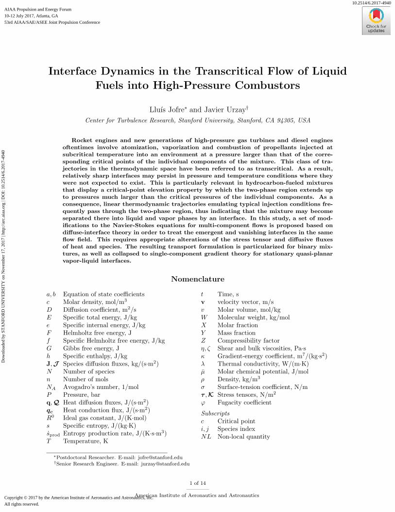
where A = aP/(R0T )2, B = bP/(R0T ), and the coefficients a and b are given by Eq. (1). Addition-ally, Z = Pv/(R0T ) is the compressibility factor, which quantifies the departures from the reference valueZ = 1 corresponding to the ideal-gas equation of state. Figure 4 shows the fugacity coefficients for an n-dodecane/nitrogen mixture at high pressure. While departures from ideality are largest at low temperatures,the chemical potential resembles that of the ideal gas for sufficiently large temperatures (e.g., above 900 K).Similar trends hold up to pressures of order 103 bar.

The transport coefficients also undergo large variations across the phase diagram at high pressures. Thetransition from liquid-like to gas-like characteristics prevent the utilization of simple expressions for the

8 of 14

American Institute of Aeronautics and Astronautics

Dow

nloa

ded

by S

TA

NFO

RD

UN

IVE

RSI

TY

on

Nov

embe

r 17

, 201

7 | h

ttp://

arc.

aiaa

.org

| D

OI:

10.

2514

/6.2

017-

4940

Figure 4. Logarithm of the n-dodecane (left panel) and nitrogen (right panel) fugacity coefficients as a function oftemperature and fuel mass fraction for an n-dodecane/nitrogen mixture at P = 100 bar.

evaluation of mixture’s viscosity, thermal conductivity and diffusion coefficients. Instead, the method inRef.27 is typically used to evaluate viscosity and thermal conductivity as function of T and ρ, whereasdiffusion coefficients can be calculated, for example, following the expressions given in Chapter 11 in Ref.28

for high-pressure conditions. These coefficients, however, are currently subject to large uncertainties.

III.C. Transport fluxes

The system of conservation equations (5)-(8) requires closure expressions for τ , K, qc, Q, Ji, and Ji. Thisis achieved through the method of irreversible thermodynamics by specifying constitutive relations suchthat the entropy production is non-negative. This methodology requires that one finds the conservationequation of entropy guided by the fact that the source terms are written as a sum of products of fluxes andthermodynamic forces.31 The formulation is greatly simplified when κij does not depend on temperature,in such a way that κeij = κij and κsij = 0, as implied by Eq. (4). In view of the experimental correlation(3), this is an approximation that has an unclear physical justification but has however been used in theliterature22,30 and will also be followed here. Starting from the second principle of thermodynamics for amulti-component system

Tds = de+ Pd(1/ρ)−N∑i=1

(µi/Wi)dYi, (16)

and substituting the relations (2), the equation

TdsNL = deNL + PNLd(1/ρ)−N∑i=1

(µi/Wi)dYi −N∑i=1

ψi · d(∇ρi)/ρ (17)

is obtained, where

ψi =N∑j=1

κij∇ρj (18)

is an auxiliary variable. A transport equation for the specific entropy sNL can be derived by taking the ma-terial derivative of Eq. (17) and substituting the conservation equations (5)-(8) into the resulting expression,which yields

ρDsNL

Dt+∇ ·

{1T

[qc + Q−

N∑i=1

{ψi [ρi∇ · v +∇ · (Ji + Ji)]− T siJi + µiJi}]}

= sprod, (19)

9 of 14

American Institute of Aeronautics and Astronautics

Dow

nloa

ded

by S

TA

NFO

RD

UN

IVE

RSI

TY

on

Nov

embe

r 17

, 201

7 | h

ttp://

arc.

aiaa

.org

| D

OI:

10.

2514

/6.2

017-

4940

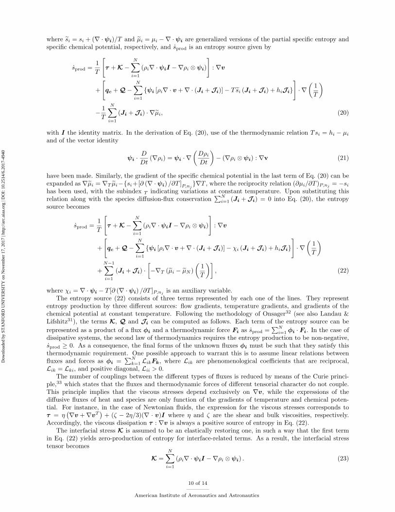
where si = si + (∇ ·ψi)/T and µi = µi −∇ ·ψi are generalized versions of the partial specific entropy andspecific chemical potential, respectively, and sprod is an entropy source given by

sprod =1T

[τ + K−

N∑i=1

(ρi∇ ·ψiI −∇ρi ⊗ψi)

]: ∇v

+

[qc + Q−

N∑i=1

{ψi [ρi∇ · v +∇ · (Ji + Ji)]− T si (Ji + Ji) + hiJi}]· ∇(

1T

)

− 1T

N∑i=1

(Ji + Ji) · ∇µi, (20)

with I the identity matrix. In the derivation of Eq. (20), use of the thermodynamic relation Tsi = hi − µiand of the vector identity

ψi ·D

Dt(∇ρi) = ψi · ∇

(DρiDt

)− (∇ρi ⊗ψi) : ∇v (21)

have been made. Similarly, the gradient of the specific chemical potential in the last term of Eq. (20) can beexpanded as ∇µi = ∇T µi−{si+[∂ (∇ ·ψi) /∂T ]P,nj

}∇T , where the reciprocity relation (∂µi/∂T )P,nj = −sihas been used, with the subindex T indicating variations at constant temperature. Upon substituting thisrelation along with the species diffusion-flux conservation

∑Ni=1 (Ji + Ji) = 0 into Eq. (20), the entropy

source becomes

sprod =1T

[τ + K−

N∑i=1

(ρi∇ ·ψiI −∇ρi ⊗ψi)

]: ∇v

+

[qc + Q−

N∑i=1

{ψi [ρi∇ · v +∇ · (Ji + Ji)]− χi (Ji + Ji) + hiJi}]· ∇(

1T

)

+N−1∑i=1

(Ji + Ji) ·[−∇T (µi − µN )

(1T

)], (22)

where χi = ∇ ·ψi − T [∂ (∇ ·ψi) /∂T ]P,njis an auxiliary variable.

The entropy source (22) consists of three terms represented by each one of the lines. They represententropy production by three different sources: flow gradients, temperature gradients, and gradients of thechemical potential at constant temperature. Following the methodology of Onsager32 (see also Landau &Lifshitz31), the terms K, Q and Ji can be computed as follows. Each term of the entropy source can berepresented as a product of a flux φi and a thermodynamic force Fi as sprod =

∑Ni=1 φi · Fi. In the case of

dissipative systems, the second law of thermodynamics requires the entropy production to be non-negative,sprod ≥ 0. As a consequence, the final forms of the unknown fluxes φi must be such that they satisfy thisthermodynamic requirement. One possible approach to warrant this is to assume linear relations betweenfluxes and forces as φi =

∑Nk=1 LikFk, where Lik are phenomenological coefficients that are reciprocal,

Lik = Lki, and positive diagonal, Lii > 0.The number of couplings between the different types of fluxes is reduced by means of the Curie princi-

ple,33 which states that the fluxes and thermodynamic forces of different tensorial character do not couple.This principle implies that the viscous stresses depend exclusively on ∇v, while the expressions of thediffusive fluxes of heat and species are only function of the gradients of temperature and chemical poten-tial. For instance, in the case of Newtonian fluids, the expression for the viscous stresses corresponds toτ = η

(∇v +∇vT

)+ (ζ − 2η/3)(∇ · v)I where η and ζ are the shear and bulk viscosities, respectively.

Accordingly, the viscous dissipation τ : ∇v is always a positive source of entropy in Eq. (22).The interfacial stress K is assumed to be an elastically restoring one, in such a way that the first term

in Eq. (22) yields zero-production of entropy for interface-related terms. As a result, the interfacial stresstensor becomes

K =N∑i=1

(ρi∇ ·ψiI −∇ρi ⊗ψi) . (23)

10 of 14

American Institute of Aeronautics and Astronautics

Dow

nloa

ded

by S

TA

NFO

RD

UN

IVE

RSI

TY

on

Nov

embe

r 17

, 201

7 | h

ttp://

arc.

aiaa

.org

| D

OI:

10.

2514

/6.2

017-

4940

Although the surface tension does not appear explicitly in Eq. (23), its effects are accounted for in the densitygradients. For a quasi-planar interface, an effective surface-tension coefficient can be defined as

σ =N∑i=1

N∑j=1

∫ +∞

−∞κij

dρidξ

dρjdξ

dξ, (24)

which, in view of Eq. (2), is proportional to the excess of free energy contained in the interface, where ξ isthe coordinate normal to the interface.24

The interfacial heat flux is cast into the form

Q =N∑i=1

{ψi [ρi∇ · v +∇ · (Ji + Ji)]− χi (Ji + Ji) + hiJi}+ Θ. (25)

The term Θ is a dissipating component that produces entropy and is computed below.In order to obtain expressions for the diffusive fluxes of heat and species, it is convenient to express

Eq. (22) in the matrix flux-force form

sprod =

[LqqF 1 +

N−1∑k=1

LqkF k+1

]· F 1 +

N−1∑i=1

[LiqF 1 +

N−1∑k=1

LikF k+1

]· F i+1, (26)

where Lqq = L1,1, Lq,k−1 = L1k (k = 2, ..., N), Li−1,q = Li1 (i = 2, ..., N), Li−1,k−1 = Lik (i, k = 2, ..., N),F 1 = ∇(1/T ) and F i>1 = −∇T (µi − µN ) (1/T ). Comparing the last two terms of Eq. (22) with Eq. (26)provides the expressions

qc = −LqqT 2∇T −

N−1∑k=1

LqkT∇T (µk − µN ) , Θ =

N−1∑k=1

LqkT∇T∇ · (ψk −ψN ) , (27)

and

Ji = −LiqT 2∇T −

N−1∑k=1

LikT∇T (µk − µN ) , Ji =

N−1∑k=1

LikT∇T∇ · (ψk −ψN ) , (28)

for the heat and species diffusion fluxes, respectively. Additionally, the relation Lqq = λT 2 is obtained byanalogy with Fourier’s law of heat conduction, with λ the thermal conductivity.

In Eqs. (23), (25) and (28), the tensor K and the fluxes Q and Ji, with Θ given in Eq. (27), representthe interfacial disturbances to the deviatoric part of the stress tensor, τ , and to the diffusive fluxes of heat,q and species Ji, respectively. In absence of interfaces, K = Q = Ji = 0 and PNL = P , thereby leading toa simplification of the conservation equations (5)-(8) to their classic Navier-Stokes form. Symmetries in thediffusive fluxes are illustrated by the presence of the Dufour term in qc due to chemical-potential gradientsas well as the corresponding Soret term in Ji due to temperature gradients.

The species diffusion flux Ji can be expanded in terms of pressure and composition gradients by makinguse of the differential form

∇T µk =(∂µk∂P

)T,Xi

∇P +N−1∑j=1

(∂µk∂Xj

)T,P,Xi6=j

∇Xj , (29)

and the Gibbs-Duhem equation

∇T µN =1XN

1c∇P −

N−1∑j=1

Xj∇T µj

, (30)

with c = ρ/W as the molar density. The combination of Eqs. (29)-(30) leads to the relation

∇T (µk − µN ) =N−1∑`=1

(X`

WNXN+δ`kWk

)N−1∑j=1

(∂µ`∂Xj

)T,P,Xi6=j

∇Xj

+

[1Wk

(∂µk∂P

)T,Xi

− 1cWNXN

+N−1∑`=1

X`

WNXN

(∂µ`∂P

)T,Xi

]∇P (31)

11 of 14

American Institute of Aeronautics and Astronautics

Dow

nloa

ded

by S

TA

NFO

RD

UN

IVE

RSI

TY

on

Nov

embe

r 17

, 201

7 | h

ttp://

arc.

aiaa

.org

| D

OI:

10.

2514

/6.2

017-

4940

for the chemical-potential gradients, where δjk is the Kronecker delta. Upon substituting Eq. (31) intoEq. (28), the species diffusion flux Ji can be expressed as

Ji = −ρ

N−1∑j=1

DMij ∇Xj +DT

i ∇T +DPi ∇P

, (32)

where DMij , DT

i and DPi are mass, thermal and pressure diffusion coefficients defined as

DMij = aiNDiN

WiXi

LiiW

N−1∑k=1

Lik

N−1∑`=1

W`X` +WNXNδ`kW`

(∂ ln f`∂Xj

)T,P,Xm6=j

, (33)

DTi = aiNDiN

kiTT, (34)

DPi = aiNDiN

WiXi

R0TLiiW

N−1∑k=1

Lik

[WNXN

WkVk −

1c

+N−1∑`=1

X`V`

], (35)

where (∂µk/∂P )T,Xi= Vk and (∂µ`/∂Xj)T,P,Xi6=j

= R0T∂ ln f`/∂Xj |T,P,Xi6=jhave been used. In Eqs. (33)-

(35), aiN = WiWN/W2 and DiN = W 2R0Lii/

(cW 2

i W2NXiXN

)are prefactors, and kiT = WiWNXiXNLiq

/(WR0Lii

)is the thermal-diffusion ratio.

Table 1. Transport coefficients and fluxes for a binary mixture with κ1,2 = κ2,1 = κ2,2 = 0.

Transport coefficients

Fickian DM1,1 = a1,2D1,2

„∂ ln f1

∂ lnX1

«T,P

Barodiffusion DP1 = a1,2D1,2

X1

R0T

„V1 −

W1

ρ

«Soret DT

1 = a1,2D1,2k1T

T

Dufour DF1 =

DT1 WR0T

W1W2X1(1−X1)

„∂ ln f1

∂ lnX1

«T,P

Interfacial (species) DK,M1 = a1,2D1,2κ1,1

W1W2X1(1−X1)

WR0T

Interfacial (heat) DK,T1 = a1,2D1,2κ1,1

k1T

TTotal stress tensor −PNLI + τ + K

Non-local pressure tensor −PNLI = −„P −

1

2κ1,1|∇ρ1|2

«I

Viscous stress tensor τ = η“∇v +∇vT

”+

„ζ −

2

3η

«(∇ · v)I

Interfacial stress tensor K = κ1,1(ρ1∇2ρ1I −∇ρ1 ⊗∇ρ1)

Total heat flux q + Q

Fourier, inter-diffusion q = −λ∇T + (h1 − h2)J1 − ρDF1 ∇X1

and Dufour heat fluxes

Interfacial heat flux Q = κ1,1∇ρ1 [ρ1∇ · v +∇ · (J1 + J1)]

−χ1(J1 + J1) + (h1 − h2)J1 + ρDK,T1 ∇T∇2ρ1

Total species diffusion flux J1 + J1

Fickian, barodiffusion J1 = −ρDM1,1∇X1 − ρDP

1 ∇P − ρDT1 ∇T

and Soret species diffusion flux

Interfacial species diffusion flux J1 = ρDK,M1 ∇T∇2

ρ1

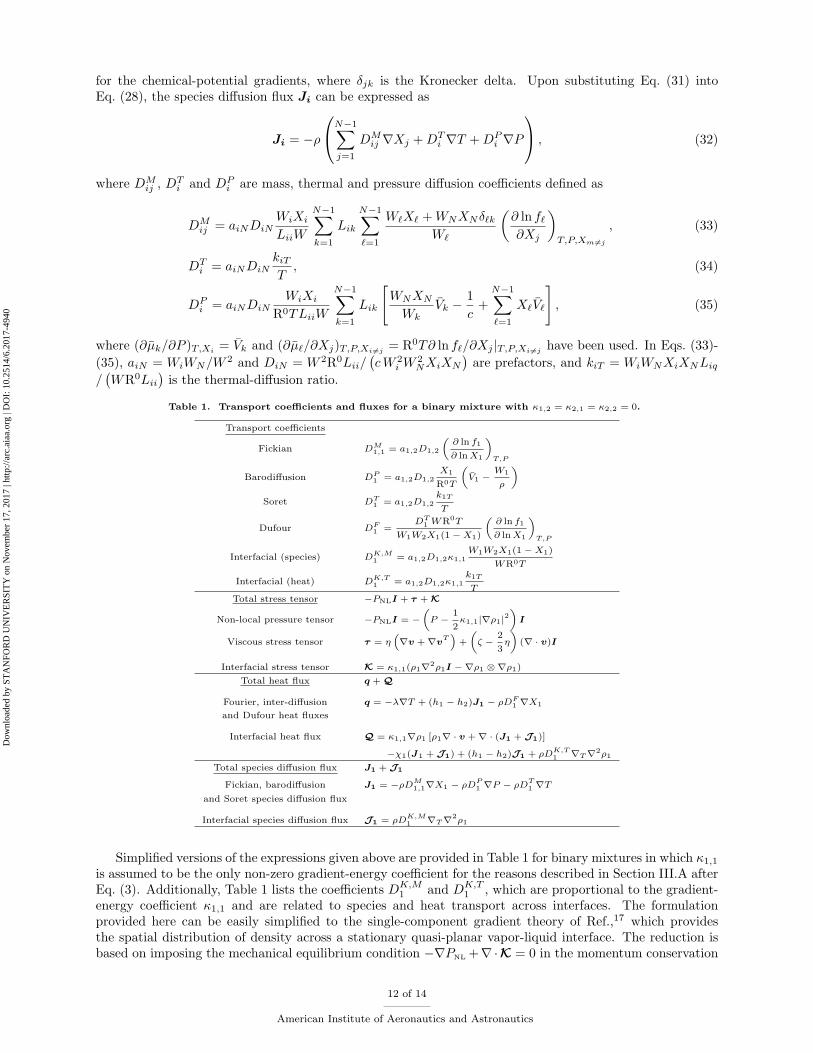
Simplified versions of the expressions given above are provided in Table 1 for binary mixtures in which κ1,1

is assumed to be the only non-zero gradient-energy coefficient for the reasons described in Section III.A afterEq. (3). Additionally, Table 1 lists the coefficients DK,M

1 and DK,T1 , which are proportional to the gradient-

energy coefficient κ1,1 and are related to species and heat transport across interfaces. The formulationprovided here can be easily simplified to the single-component gradient theory of Ref.,17 which providesthe spatial distribution of density across a stationary quasi-planar vapor-liquid interface. The reduction isbased on imposing the mechanical equilibrium condition −∇PNL +∇·K = 0 in the momentum conservation

12 of 14

American Institute of Aeronautics and Astronautics

Dow

nloa

ded

by S

TA

NFO

RD

UN

IVE

RSI

TY

on

Nov

embe

r 17

, 201

7 | h

ttp://

arc.

aiaa

.org

| D

OI:

10.

2514

/6.2

017-

4940

equation (6), with PNL and K being defined in Eqs. (9) and (23), respectively. This constraint leads to thegradient-theory equation

P − P0 = κρd2ρ

dξ2− 1

2κ

(dρ

dξ

)2

, (36)

where ξ is the coordinate normal to the interface and P0 the thermodynamic pressure far from the interface.Integration of Eq. (36), subject to far-field boundary conditions for the vapor- and liquid-phase densities,yields ρ(ξ) across the interface. Further details on the integration of Eq. (36) can be found, for instance, inRef.34

IV. Conclusions

This study focuses on theoretical aspects of transcritical dynamics of liquid-fuel streams injected intohigh-pressure environments. The mixture displays a critical-point elevation property by which the two-phase region extends up to pressures much larger than the critical pressures of the individual components.As a result, linear thermodynamic trajectories emulating typical injection conditions frequently pass throughthe two-phase region, thus indicating that the mixture could become separated into liquid and vapor phasesby an interface. A set of modifications to the Navier-Stokes equations for multi-component flows is proposedbased on diffuse-interface theory in order to treat the emergent and vanishing interfaces in the same flowfield. This requires appropriate alterations of the stress tensor and diffusive fluxes of heat and species. Theresulting transport formulation is particularized for binary mixtures and single-component flows, the latterrecovering the well-known gradient theory of van der Waals.17

It should be mentioned that in most practical cases the computational cost of the numerical resolutionof the resulting interfaces would be prohibitive, since they typically remain small with respect to the hy-drodynamic scales (e.g., see resulting thicknesses based on the one-dimensional gradient theory in Ref.20).Nonetheless, this should not deter the derivation and understanding of formulations that may be later usedto inspire subgrid-scale interface-modeling approaches. Future work will involve the integration of theseequations in simple canonical problems.

Acknowledgments

This investigation was funded by the US AFOSR, Grant #FA9550-15-C-0037.

References

1Oefelein, J. C. & Yang, V. 1993 Comprehensive review of liquid-propellant combustion instabilities in F-1 engines. J.Propul. Power 9, 657–677.

2Rosner, D. E. 1972 Liquid droplet vaporization and combustion. In Liquid Propellant Rocket Combustion Instability,Harrje, D. T. and Reardon H. (Eds.) NASA.

3Sirignano, W. A. & Delplanque, J. P. 1999 Transcritical vaporization of liquid fuels and propellants. J. Propul. Power 15,806–902.

4Dahms, R. N., Manin, J., Pickett, L. M. & Oefelein, J. C. 2013 Understanding high-pressure gas-liquid interface phenomenain diesel engines. Proc. Combust. Inst. 34, 1667–1675.

5Lasheras, J. C & Hopfinger, E. J. 2000 Liquid jet instability and atomization. Annu. Rev. Fluid Mech. 32, 275–308.6Sanchez, A. L., Urzay, J. & Linan, A. 2015 The role of separation of scales in the description of spray combustion. Proc.

Combust. Inst. 35, 1549–1577.7Gaillard, P., Giovangigli, V. & Matuszewski, L. 2016 A diffuse interface LOX/hydrogen transcritical flame model. Combust.

Theor. Model. 20, 486–520.8Manin, J., Bardi, M., Pickett, L. M., Dahms, R. N. & Oefelein, J. C. 2014 Microscopic investigation of the atomization

and mixing processes of diesel sprays injected into high pressure and temperature environments. Fuel 134, 531–543.9Qiu, L. & Reitz, R. D. 2015 An investigation of thermodynamic states during high-pressure fuel injection using equilibrium

thermodynamics. Int. J. Multiphase Flow 72, 24–38.10Firoozabadi, A. 2015 Thermodynamics and Applications in Hydrocarbon Energy Production. McGraw-Hill.11Heidemann, R. A. & Khalil, A. M. 1980 The calculation of critical points. AIChE J. 26, 769–779.12Peng, D.-Y. & Robinson, D. B. 1976 A new two-constant equation of state. Ind. Eng. Chem. Fundam. 15, 59–64.13Harstad, K. G., Miller, R. S. & Bellan, J. 1997 Efficient high-pressure state equations. AIChE J. 43, 1605–1610.14Garcıa-Cordova, T., Justo-Garcıa, D. N., Garcıa-Flores, B. E. & Garcıa-Sanchez, F. 2011 Vapor-liquid equilibrium data

for the Nitrogen + Dodecane system at temperatures from (344 to 593) K and at pressures up to 60 MPa. J. Chem. Eng. Data56, 1555–1564.

13 of 14

American Institute of Aeronautics and Astronautics

Dow

nloa

ded

by S

TA

NFO

RD

UN

IVE

RSI

TY

on

Nov

embe

r 17

, 201

7 | h

ttp://

arc.

aiaa

.org

| D

OI:

10.

2514

/6.2

017-

4940

15van Konynenburg, P. H. & Scott, R. L. 1980 Critical lines and phase equilibria in binary van der Waals mixtures. Philos.Trans. Royal Soc. Lond. A 298, 495–540.

16Matheis, J. & Hickel S. 2016 Multi-component vapor-liquid equilibrium model for LES and application to ECN Spray A.Proceedings of the Summer Program, Center for Turbulence Research, Stanford University, pp. 25–34.

17van der Waals, J. D. 1893 The thermodynamic theory of capillarity under the hypothesis of a continuous variation ofdensity. Translated by J. S. Rowlinson 1979 J. Stat. Phys. 20, 197–244.

18Cahn, J. W. & Hilliard, J. E. 1958 Free energy of a nonuniform system. I. Interfacial free energy. J. Chem. Phys. 28,258–267.

19Anderson, D. M., McFadden, G. B. & Wheeler, A. A. 1998 Diffuse-interface methods in fluid mechanics. Annu. Rev.Fluid Mech. 30, 139–165.

20Dahms, R. N. & Oefelein, J. C. 2013 On the transition between two-phase and single-phase interface dynamics inmulticomponent fluids at supercritical pressures. Phys. Fluids 25, 092103.

21Dunn, J. E. & Serrin, J. 1985 On the thermomechanics of interstitial working. Arch. Ration. Mech. Anal. 88, 95–133.22Pismen, L. M. 2001 Nonlocal diffuse interface theory of thin films and the moving contact line. Phys. Rev. E 64, 021603.23Rowlinson, J. S. & Widow, B. 2002 Molecular Theory of Capillarity. Dover.24Lin, H., Duan, Y.-Y. & Min, Q. 2007 Gradient theory modeling of surface tension for pure fluids and binary mixtures.

Fluid Phase Equilib. 254, 75–90.25Benedict, M., Webb, G. B. & Rubin, L. C. 1942 An empirical equation for thermodynamic properties of light hydrocarbons

and their mixtures II. Mixtures of methane, ethane, propane, and n-butane. J. Chem. Phys. 10, 747–758.26Soave, G. 1972 Equilibrium constants from a modified Redlich-Kwong equation of state. Chem. Eng. Sci. 27, 1197–1203.27Chung, T. H., Ajlan, M., Lee, L. L. & Starling, K. E. 1988 Generalized multiparameter correlation for nonpolar and polar

fluid transport properties. Ind. Eng. Chem. Fundam. 27, 671–679.28Poling, B. E., Prausnitz, J. M. & O’Connel, J. P. 2001 The Properties of Gases and Liquids. McGraw-Hill.29Miller, R. S. 2000 Long time mass fraction statistics in stationary compressible isotropic turbulence at supercritical

pressure. Phys. Fluids 12, 2020–2032.30Papatzacos, P. 2000 Diffuse-interface models for two-phase flow. Physica Scripta 61, 349–360.31Landau, L. D. & Lifshitz, E. M. 1987 Course of Theoretical Physics: Fluid mechanics. Pergamon Press.32Onsager, L. 1931 Reciprocal relations in irreversible processes. I. Phys. Rev. 37, 405–426.33Curie, P. 1894 Sur la symetrie des phenomenes physiques: symetrie d’un champ electrique et d’un champ magnetique. J.

Phys. 3, 393–415.34Jofre, L., Urzay, J., Mani, A. & Moin, P. 2015 On diffuse-interface modeling of high-pressure transcritical fuel sprays.

Annual Research Briefs, Center for Turbulence Research, Stanford University, 55–64.

14 of 14

American Institute of Aeronautics and Astronautics

Dow

nloa

ded

by S

TA

NFO

RD

UN

IVE

RSI

TY

on

Nov

embe

r 17

, 201

7 | h

ttp://

arc.

aiaa

.org

| D

OI:

10.

2514

/6.2

017-

4940