Interest Rate Models: Paradigm shifts in recent yearsieor.columbia.edu/files/seasdepts/industrial-engineering... · Interest Rate Models: Paradigm shifts in recent years Damiano Brigo

Interest Rate Models: Paradigm shifts in recent years

Damiano BrigoQ-SCI, Managing Director and Global Head

DerivativeFitch, 101 Finsbury Pavement, London

Columbia University Seminar, New York, November 5, 2007

This presentation is based on the book

”Interest Rate Models: Theory and Practice - with Smile, Inflation and Credit”

by D. Brigo and F. Mercurio, Springer-Verlag, 2001 (2nd ed. 2006)

http://www.damianobrigo.it/book.html

Damiano Brigo, Q-SCI, DerivativeFitch, London Columbia University Seminar, November 5, 2007

Overview

• No arbitrage and derivatives pricing.

• Modeling suggested by no-arbitrage discounting.1977: Endogenous short-rate term structure models

• Reproducing the initial market interest-rate curve exactly.1990: Exogenous short rate models

• A general framework for no-arbitrage rates dynamics.1990: HJM - modeling instantaneous forward rates

• Moving closer to the market and consistency with market formulas1997: Fwd market-rates models calibration and diagnostics power

• 2002: Volatility smile extensions of Forward market-rates models

Interest rate models: Paradigms shifts in recent years 1


No arbitrage and Risk neutral valuation

Recall shortly the risk-neutral valuation paradigm of Harrison and Pliska’s(1983), characterizing no-arbitrage theory:

A future stochastic payoff, built on an underlying fundamental financialasset, paid at a future time T and satisfying some technical conditions, hasas unique price at current time t the risk neutral world expectation

EQt

exp

(−

∫ T

t

rs ds

)

︸︷︷︸Payoff(Asset)T

Stochastic discount factor

where r is the risk-free instantaneous discount rate



Risk neutral valuation

EQt

[exp

(−

∫ T

t

rs ds

)Payoff(Asset)T

]

“Risk neutral world” means that all fundamental underlying assets musthave as locally deterministic drift rate (expected return) the risk-free interestrate r:

d AssettAssett

= rt dt + Asset-%-Volatilityt (0−mean dt−variance Normal shock under Q)t

Nothing strange at first sight. To value future unknown quantities now,we discount at the relevant interest rate and then take expectation, andthe mean is a reasonable estimate of unknown quantities.




But what is surprising is that we do not take the mean in the realworld (statistics, econometrics) but rather in the risk neutral world, sincethe actual growth rate of our asset (e.g. a stock) in the real world doesnot enter the price and is replaced by the risk free rate r.

d AssettAssett

= rt︸︷︷︸dt + Asset-%-Volatilityt (0−mean dt−variance Normal shock under Q)t

risk free rate

Even if two investors do not agree on the expected return of afundamental asset in the real world, they still agree on the price ofderivatives (e.g. options) built on this asset.




This is one of the reasons for the enormous success of Option pricingtheory, and partly for the Nobel award to Black, Scholes and Merton whostarted it.

According to Stephen Ross (MIT) in the Palgrave Dictionary ofEconomics:”... options pricing theory is the most successful theory not only infinance, but in all of economics”.

From the risk neutral valuation formula we see that one fundamentalquantity is rt, the instantaneous interest rate. In particular, if we takePayoffT = 1, we obtain the Zero-Coupon Bond



Zero-coupon Bond, LIBOR rate

A T–maturity zero–coupon bond guarantees the payment of one unitof currency at time T . The contract value at time t < T is denoted byP (t, T ):

P (T, T ) = 1, P (t, T ) = EQt

[exp

(−

∫ T

t

rs ds

)1

]t ←− T↓ ↓

P (t, T ) 1

All kind of rates can be expressed in terms of zero–coupon bonds andvice-versa. ZCB’s can be used as fundamental quantities or building blocksof the interest rate curve.



Zero-coupon Bond, LIBOR and swap rates

• Zero Bond at t for maturity T : P (t, T ) = Et

[exp

(− ∫ T

trs ds

)]

• Spot LIBOR rate at t for maturity T : L(t, T ) = 1−P (t,T )(T−t) P (t,T );

• Fwd Libor at t, expiry Ti−1 maturity Ti: Fi(t) := 1Ti−Ti−1

(P (t,Ti−1)P (t,Ti)

− 1).

This is a market rate, it underlies the Fwd Rate Agreement contracts.

• Swap rate at t with tenor Tα, Tα+1, . . . , Tβ. This is a market rate- itunderlies the Interest Rate Swap contracts:

Sα,β(t) :=P (t, Tα)− P (t, Tβ)∑β

i=α+1(Ti − Ti−1)P (t, Ti).



Zero-coupon Bond, LIBOR and swap rates

L(t, Tj), Fi(t), Sα,β(t), .... these rates at time t, for different maturitiesT = Tj, Ti−1, Ti, Tα, Tβ, are completely known from bonds T 7→ P (t, T ).

Bonds in turn are defined by expectations of functionals of future pathsof rt. So if we know the probabilistic behaviour of r from time t on, wealso know the bonds and rates for all maturities at time t:

term structure at time t : T 7→ L(t, T ), initial point rt ≈ L(t, t+small ε)

drt future random dynamics ⇒ Knowledge of T 7→ L(t, T ) at t;

T 7→ L(t, T ) at t ⇒/ Knowledge of drt random future dynamics;



Zero-coupon curve

5 10 15 20 25 304.4%

4.6%

4.8%

5%

5.2%

5.4%

5.6%

5.8%

6%

Maturity (in years)

Rat

e

Figure 1: Zero-coupon curve T 7→ L(t, t + T ) stripped from market EUROrates on February 13, 2001, T = 0, . . . , 30y



Which variables do we model?

The curve today does not completely specify how rates will move in thefuture. For derivatives pricing, we need specifying a stochastic dynamics forinterest rates, i.e. choosing an interest-rate model.

• Which quantities dynamics do we model? Short rate rt? LIBOR L(t, T )?Forward LIBOR Fi(t)? Forward Swap Sα,β(t)? Bond P (t, T )?

• How is randomness modeled? i.e: What kind of stochastic process orstochastic differential equation do we select for our model?

• Consequences for valuation of specific products, implementation,goodness of calibration, diagnostics, stability, robustness, etc?



First Choice: short rate r (Vasicek, 1977)

This approach is based on the fact that the zero coupon curve at anyinstant, or the (informationally equivalent) zero bond curve

T 7→ P (t, T ) = EQt exp

(−

∫ T

t

rs ds

)

is completely characterized by the probabilistic/dynamical properties of r.So we write a model for r, typically a stochastic differential equation

d rt = local mean(t, rt)dt+local standard deviation(t, rt)× 0− mean dt− variance normal shockt

which we write drt = b(t, rt)︸︷︷︸ dt + σ(t, rt)︸︷︷︸ dWt .

drift diffusion coeff. or absolute volatility



First Choice: short rate r

Dynamics of rt under the risk–neutral-world probability measure

1. Vasicek (1977): drt = k(θ − rt)dt + σdWt, α = (k, θ, σ).

2. Cox-Ingersoll-Ross (CIR, 1985):

drt = k(θ − rt)dt + σ√

rtdWt, α = (k, θ, σ), 2kθ > σ2 .

3. Dothan / Rendleman and Bartter:

drt = artdt + σrtdWt, (rt = r0 e(a−12σ2)t+σWt, α = (a, σ)).

4. Exponential Vasicek: rt = exp(zt), dzt = k(θ − zt)dt + σdWt.



First Choice: short rate r. Example: Vasicek

drt = k(θ − rt)dt + σdWt.

The equation is linear and can be solved explicitly: Good.

Joint distributions of many important quantities are Gaussian. Manyformula for prices (i.e. expectations): Good.

The model is mean reverting: The expected value of the short rate tendsto a constant value θ with velocity depending on k as time grows, while itsvariance does not explode. Good also for risk management, rating.

Rates can assume negative values with positive probability. Bad.

Gaussian distributions for the rates are not compatible with the marketimplied distributions.



First Choice: short rate r. Example: CIR

drt = k[θ − rt]dt + σ√

rt dW (t)

For the parameters k, θ and σ ranging in a reasonable region, this modelimplies positive interest rates, but the instantaneous rate is characterizedby a noncentral chi-squared distribution. The model is mean revertingas Vasicek’s.

This model maintains a certain degree of analytical tractability, but isless tractable than Vasicek

CIR is closer to market implied distributions of rates (fatter tails).

Therefore, the CIR dynamics has both some advantages anddisadvantages with respect to the Vasicek model.

Similar comparisons affect lognormal models, that however lose alltractability.



First Choice: Modeling r. Endogenous models.

Model Distrib Analytic Analytic Multifactor Mean r > 0?

P (t, T ) Options Extensions Reversion

Vasicek Gaussian Yes Yes Yes Yes No

CIR n.c. χ2, Gaussian2 Yes Yes Yes but.. Yes Yes

Dothan eGaussian ”Yes” No Difficult ”Yes” Yes

Exp. Vasicek eGaussian No No Difficult Yes Yes

These models are endogenous. P (t, T ) = Et(e−∫ Tt r(s)ds) can be

computed as an expression (or numerically in the last two) depending onthe model parameters.

E.g. in Vasicek, at t = 0, the interest rate curve is an output of themodel, rather than an input, depending on k, θ, σ, r0 in the dynamics.



First Choice: Modeling r. Endogenous models.

Given the observed curve T 7→ PMarket(0, T ) , we wish our modelto incorporate this curve. Then we need forcing the model parametersto produce a curve as close as possible to the market curve. This is thecalibration of the model to market data.

k, θ, σ, r0?: T 7→ PVasicek(0, T ; k, θ, σ, r0) is closest to T 7→ PMarket(0, T )

Too few parameters. Some shapes of T 7→ LMarket(0, T ) (like aninverted shape in the picture above) can never be obtained.

To improve this situation and calibrate also option data, exogenousterm structure models are usually considered.



First Choice: Modeling r. Exogenous models.

The basic strategy that is used to transform an endogenous model intoan exogenous model is the inclusion of “time-varying” parameters. Typically,in the Vasicek case, one does the following:

dr(t) = k[θ− r(t)]dt + σdW (t) −→ dr(t) = k[ ϑ(t) − r(t)]dt + σdW (t) .

ϑ(t) can be defined in terms of T 7→ LMarket(0, T ) in such a way that themodel reproduces exactly the curve itself at time 0.

The remaining parameters may be used to calibrate option data.



1. Ho-Lee: drt = θ(t) dt + σ dWt.

2. Hull-White (Extended Vasicek): drt = k(θ(t)− rt)dt + σdWt.

3. Black-Derman-Toy (Extended Dothan): rt = r0 eu(t)+σ(t)Wt

4. Black-Karasinski (Extended exponential Vasicek):

rt = exp(zt), dzt = k [θ(t)− zt] dt + σdWt.

5. CIR++ (Shifted CIR model, Brigo & Mercurio ):

rt = xt + φ(t; α), dxt = k(θ − xt)dt + σ√

xtdWt

In general other parameters can be chosen to be time–varying so as toimprove fitting of the volatility term–structure (but...)



Extended Distrib Analytic Analytic Multifactor Mean r > 0?Model bond form. Analytic extension ReversionHo-Lee Gaussian Yes Yes Yes No No

Hull-White Gaussian Yes Yes Yes Yes No

BDT eGaussian No No difficult Yes Yes

BK eGaussian No No difficult Yes YesCIR++ s.n.c. χ2 Yes Yes Yes Yes Yes but..

≈ Gaussian2

Tractable models are more suited to risk management thanks tocomputational ease and are still used by many firms

Pricing models need to be more precise in the distribution properties solognormal models were usually preferred (BDT, BK). For pricing these havebeen supplanted in large extent by our next choices below.



First choice: Modeling r. Multidimensional models

In these models, typically (e.g. shifted two-factor Vasicek)

dxt = kx(θx − xt)dt + σxdW1(t),

dyt = ky(θy − yt)dt + σydW2(t), dW1 dW2 = ρ dt,

rt = xt + yt + φ(t, α), α = (kx, θx, σx, x0, ky, θy, σy, y0)

More parameters, can capture more flexible options structures and especiallygive less correlated rates at future times: 1-dimens models havecorr(L(1y, 2y), L(1y, 30y)) = 1, due to the single random shock dW .Here we may play with ρ in the two sources of randomness W1 and W2.

We may retain analytical tractability with this Gaussian version, whereasLognormal or CIR can give troubles.



First choice: Modeling r. Numerical methods

Monte Carlo simulation is the method for payoffs that are path dependent(range accrual, trigger swaps...): it goes forward in time, so at any time itknows the whole past history but not the future.

Finite differences or recombining lattices/trees: this is the method forearly exercise products like american or bermudan options. It goes back intime and at each point in time knows what will happen in the future butnot in the past.

Monte carlo with approximations of the future behaviour regressed onthe present (Least Squared Monte Carlo) is the method for products bothpath dependent and early exercise (e.g. multi callable range accrual).



Figure 2: A possible geometry for the discrete-space discrete-time treeapproximating r.



0 1 2 3 4 5 6 7 8 9 100.025

0.03

0.035

0.04

0.045

0.05

0.055

0.06

Figure 3: Five paths for the monte carlo simulation of r



0 1 2 3 4 5 6 7 8 9 100.025

0.03

0.035

0.04

0.045

0.05

0.055

0.06

0.065

Figure 4: 100 paths for the monte carlo simulation of r



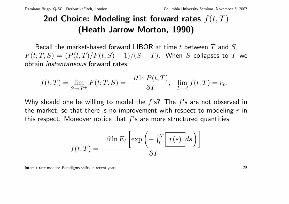
2nd Choice: Modeling inst forward rates f(t, T )(Heath Jarrow Morton, 1990)

Recall the market-based forward LIBOR at time t between T and S,F (t; T, S) = (P (t, T )/P (t, S) − 1)/(S − T ). When S collapses to T weobtain instantaneous forward rates:

f(t, T ) = limS→T+

F (t; T, S) = −∂ ln P (t, T )∂T

, limT→t

f(t, T ) = rt.

Why should one be willing to model the f ’s? The f ’s are not observed inthe market, so that there is no improvement with respect to modeling r inthis respect. Moreover notice that f ’s are more structured quantities:

f(t, T ) = −∂ ln Et

[exp

(− ∫ T

tr(s) ds

)]

∂T



Second Choice: Modeling inst forward rates f(t, T )

Given the rich structure in r, we expect restrictions on the dynamicsthat are allowed for f . Indeed, there is a fundamental theoretical result due

to Heath, Jarrow and Morton (HJM, 1990): Set f(0, T ) = fMarket(0, T ).We have

df(t, T ) = σ(t, T )

(∫ T

t

σ(t, s)ds

)dt + σ(t, T )dW (t),

under the risk neutral world measure, if no arbitrage has to hold. Thus wefind that the no-arbitrage property of interest rates dynamics is here clearlyexpressed as a link between the local standard deviation (volatility ordiffusion coefficient) and the local mean (drift) in the dynamics.



Second Choice: Modeling inst forward rates f(t, T )

df(t, T ) = σ(t, T )

(∫ T

t

σ(t, s)ds

)dt + σ(t, T )dW (t),

Given the volatility, there is no freedom in selecting the drift, contraryto the more fundamental models based on drt, where the whole risk neutraldynamics was free:

drt = b(t, rt)dt + σ(t, rt)dWt

b and σ had no link due to no-arbitrage.



Second Choice, modeling f (HJM): retrospective

Useful to study arbitrage free properties, but when in need of writinga concrete model, most useful models coming out of HJM are the alreadyknown short rate models seen earlier (these are particular HJM models,especially exogenous Gaussian models) or the market models we see later.

r model → HJM → Market models (LIBOR and SWAP)Risk Management, ??? Accurate Pricing, HedgingRating, easy pricing ??? Accurate Calibration, vol Smile

HJM may serve as a unifying framework in which all categories ofno-arbitrage interest-rate models can be expressed.



Third choice: Modeling Market rates.The LIBOR amd SWAP MARKET MODELS (1997)

Recall the forward LIBOR rate at time t between Ti−1 and Ti,

Fi(t) = (P (t, Ti−1)/P (t, Ti)− 1)/(Ti − Ti−1),

associated to the relevant Forward Rate Agreement. A family of Fi withspanning i is modeled in the LIBOR market model instead of r or f .

To further motivate market models, let us consider the time-0 priceof a T2-maturity libor rate call option - caplet - resetting at time T1

(0 < T1 < T2) with strike X. Let τ denote the year fraction between T1

and T2. Such a contract pays out at time T2 the amount

τ(L(T1, T2)−X)+ = τ(F2(T1)−X)+.



Third Choice: Market models.

E

exp

(−

∫ T2

0

rsds

)

︸︷︷︸τ (L(T1, T2)−X)+︸︷︷︸

= P (0, T2)EQ2

[τ(F2(T1)−X)+],

Discount from 2 years Call option on Libor(1year,2years)

(change to measure Q2 associated to numeraire P (t, T2), leading to adriftless F2) with a lognormal distribution for F :

dF2(t) = v F2(t)dW2(t), mkt F2(0)

where v is the instantaneous volatility, and W2 is a standard Brownianmotion under the measure Q2.




Then the expectation EQ2[(F2(T1)−X)+] can be viewed as a T1-

maturity call-option price with strike X and underlying volatility v.

The zero-curve T 7→ L(0, T ) is calibrated through the market Fi(0)’s.We obtain from lognormality of F:

Cpl(0, T1, T2, X) := P (0, T2) τ E(F2(T1)−X)+

= P (0, T2)τ [ F2(0) N(d1(X, F2(0), v√

T1)) − X N(d2(X,F2(0), v√

T1))],

d1,2(X, F, u) =ln(F/X)± u2/2

u,

where N is the standard Gaussian cumulative distribution function. Thisis the Black formula that has been used in the market for years to convertprices Cpl in volatilities v and vice-versa.




The LIBOR market model is thus compatible with Black’s market formulaand indeed prior to this model there was no rigorous arbitrage freejustification of the formula, a building block for all the interest rateoptions market.

A similar justification for the market swaption formula is obtainedthrough the swap market model, where forward swap rates Sα,β(t) aremodeled as lognormal processes each under a convenient measure.

LIBOR and SWAP market models are inconsistent in theory butconsistent in practice.




The quantities in the LIBOR market models are forward rates comingfrom expectations of objects involving r, and thus are structured.

As for HJM, we may expect restrictions when we write their dynamics.

We have already seen that each Fi has no drift (local mean) under itsforward measure. Under other measures, like for example the (discrete tenoranalogous of the) risk neutral measure, the Fi have local means comingfrom the volatilities and correlations of the family of forward rates F beingmodeled.




This is similar to HJM

dFk(t) = σk(t) Fk(t)k∑

j:Tj>t

τj ρj,k σj(t) Fj(t)

1 + τjFj(t)︸︷︷︸

dt + σk(t) Fk(t) dZk(t)

local mean or drift

′′volatility′′(dFj(t)) = σj(t) , ′′correlation′′(dFi, dFj) = ρi,j .




′′volatility′′(dFj(t)) = σj(t) , ′′correlation′′(dFi, dFj) = ρi,j .

This direct modeling of vol and correlation of the movement of realmarket rates rather than of abstract rates like r or f is one of the reasonsof the success of market models.

Vols and correlations refer to objects the trader is familiar with.

On the contrary the trader may have difficulties in translating a dynamicsof r in facts referring directly to the market. Questions like ”what is thevolatility of the 2y3y rate” or ”what is the correlation between the 2y3y andthe 9y10y rates” are more difficult with r models.




Furthermore r models are not consistent with the market standardformulas for options.

Also, market models allow easy diagnostics and extrapolation of thevolatility future term structure and of terminal correlations that are quitedifficult to obtain with r models.

Not to mention that the abundance of clearly interpretable parametersmakes market models able to calibrate a large amount of option data, atask impossible with reasonable short rate r models.

The model can easily account for 130 swaptions volatilities consistently.



The most recent paradigm shift: Smile Modeling

In recent years, after influencing the FX and equity markets, the volatilitysmile effect has entered also the interest rate market.

The volatility smile affects directly volatilities associated with optioncontracts such as caplets and swaptions, and is expressed in terms ofmarket rates volatilities. For this reason, models addressing it are morenaturally market models than r models or HJM.



Smile Modeling: Introduction

The option market is largely built around Black’s formula. Recall theT2-maturity caplet resetting at T1 with strike K. Under the lognormalLIBOR model, its underlying forward follows

dF2(t) = σ2(t)F2(t)dW2(t)

with deterministic time dependent instantaneous volatility σ2 not dependingon the level F2. Then we have Black’s formula

CplBlack(0, T1, T2,K) = P (0, T2)τBlack(K, F2(0), v2(T1)), v2(T1)2 =1T1

∫ T1

0

σ22(t)dt .

Volatility is a characteristic of the underlying and not of the contract.Therefore the averaged volatility v2(T1) should not depend on K.



Smile Modeling: The problem

Now take two different strikes K1 and K2 for market quoted options.Does there exist a single volatility v2(T1) such that both

CplMKT(0, T1, T2,K1) = P (0, T2)τBlack(K1, F2(0), v2(T1))

CplMKT(0, T1, T2,K2) = P (0, T2)τBlack(K2, F2(0), v2(T1))

hold? The answer is a resounding “no”. Two different volatilities v2(T1,K1)and v2(T1,K2) are required to match the observed market prices if one isto use Black’s formula



Smile Modeling: The problem

CplMKT(0, T1, T2,K1) = P (0, T2)τBlack(K1, F2(0), vMKT2 (T1,K1)),

CplMKT(0, T1, T2,K2) = P (0, T2)τBlack(K2, F2(0), vMKT2 (T1,K2)).

Each caplet market price requires its own Black volatility vMKT2 (T1,K)

depending on the caplet strike K.

The market therefore uses Black’s formula simply as a metric to expresscaplet prices as volatilities, but the dynamic and probabilistic assumptionsbehind the formula, i.e. dF2(t) = σ2(t)F2(t)dW2(t), do not hold.

The typically smiley shape curve K 7→ vMKT2 (T1,K) is called the

volatility smile.



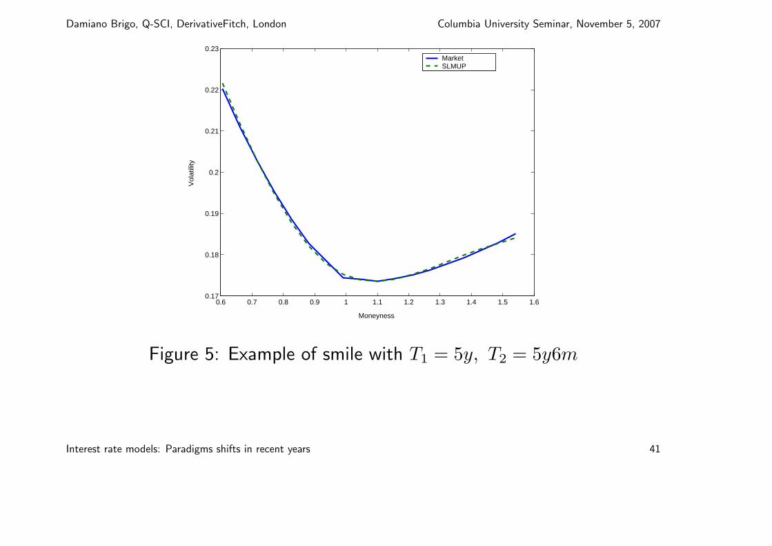
0.6 0.7 0.8 0.9 1 1.1 1.2 1.3 1.4 1.5 1.60.17

0.18

0.19

0.2

0.21

0.22

0.23

Moneyness

Vol

atili

ty

MarketSLMUP

Figure 5: Example of smile with T1 = 5y, T2 = 5y6m



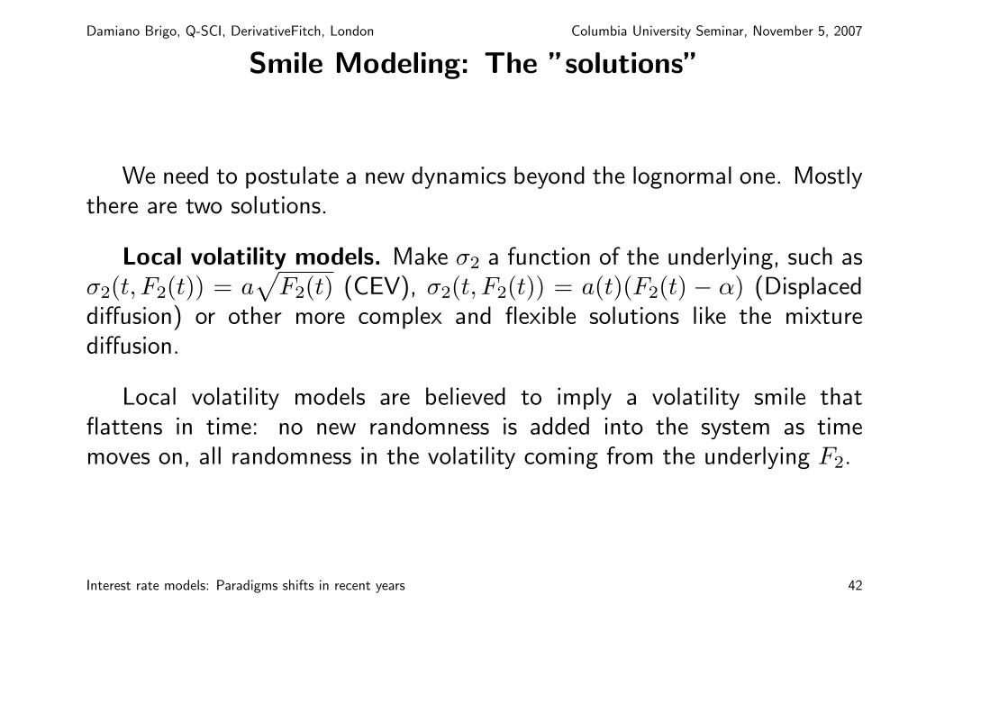
Smile Modeling: The ”solutions”

We need to postulate a new dynamics beyond the lognormal one. Mostlythere are two solutions.

Local volatility models. Make σ2 a function of the underlying, such asσ2(t, F2(t)) = a

√F2(t) (CEV), σ2(t, F2(t)) = a(t)(F2(t) − α) (Displaced

diffusion) or other more complex and flexible solutions like the mixturediffusion.

Local volatility models are believed to imply a volatility smile thatflattens in time: no new randomness is added into the system as timemoves on, all randomness in the volatility coming from the underlying F2.




Stochastic volatility models. Make σ2 a new stochastic process,adding new randomness to the volatility, so that in a way volatility becomesa variable with a new random life of its own, possibly correlated with theunderlying. Heston’s model (1993), adapted to interest rates by Wu andZhang (2002):)

dF2(t) =√

v(t)F2(t)dW2(t),

dv(t) = k(θ − v(t))dt + η√

v(t)dZ2(t), dZdW = ρdt.




A different, more simplistic and popular stochastic volatility model is theso-called SABR (2002):

dF2(t) = b(t)(F2(t))βdW2(t),db(t) = νb(t)dZ2(t), b0 = α, dZdW = ρ dt

with 0 < β ≤ 1, ν and α positive. Analytical approximations provideformulas in closed form. When applied to swaptions, this model has beenused to quote and interpolate implied volatilities in the swaption marketacross strikes.

Finally, uncertain volatility models where σ2 takes at random one amongsome given values are possible, and lead to models similar to the mixturediffusions in the local volatility case.



Conclusions

1977: short rate models drt

1990: HJM df(t, T )

1997: Market models dFi(t), dSα,β(t)

2002: Volatility smile inclusive Market models dFi(t), dSα,β(t)

All these formulations are still operating on different levels, ranging fromrisk management to rating practice to advanced pricing.

The models have different increasing levels of complexity but in somerespects, while having richer parameterization, dFi market models are moretransparent than simpler dr models.

No family of models wins across the whole spectrum of applications andall these models are still needed for different applications.


Documents

Interest Rate Models: Paradigm shifts in recent yearsieor.columbia.edu/files/seasdepts/industrial-engineering... · Interest Rate Models: Paradigm shifts in recent years Damiano Brigo