Embed Size (px)
Citation preview
Nelson–Siegel Models No arbitrage models HJM = NSproj +Adj , Adj small
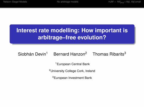
Interest rate modelling: How important isarbitrage–free evolution?
Siobhán Devin1 Bernard Hanzon2 Thomas Ribarits3
1European Central Bank
2University College Cork, Ireland
3European Investment Bank
Nelson–Siegel Models No arbitrage models HJM = NSproj +Adj , Adj small
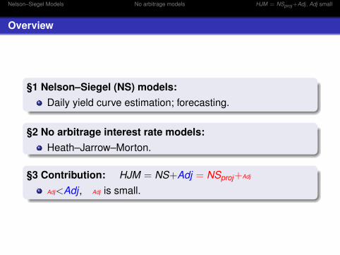
Overview
§1 Nelson–Siegel (NS) models:Daily yield curve estimation; forecasting.
§2 No arbitrage interest rate models:Heath–Jarrow–Morton.
§3 Contribution: HJM = NS+Adj = NSproj+Adj
Adj<Adj , Adj is small.
Nelson–Siegel Models No arbitrage models HJM = NSproj +Adj , Adj small
Some notation
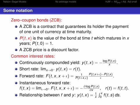
Zero–coupon bonds (ZCB):A ZCB is a contract that guarantees its holder the paymentof one unit of currency at time maturity.P(t , x) is the value of the bond at time t which matures in xyears; P(t ,0) = 1.A ZCB price is a discount factor.
Common interest rates:Continuously compounded yield: y(t , x) = − log P(t ,x)
x .Short rate: limx→0+ y(t , x) = r(t).
Forward rate: F (t , x , x + ε) = 1P(t+x ,ε)
P(t ,x+ε)−P(t ,x)ε .
Instantaneous forward rate:f (t , x) = limε→0+ F (t , x , x + ε) = −∂ log P(t ,x)
∂x , r(t) = f (t , t).
Relationship between f and y : y(t , x) = 1x
∫ x0 f (t , s) ds.
Nelson–Siegel Models No arbitrage models HJM = NSproj +Adj , Adj small
§1 Nelson–Siegel (NS) models
§1 Nelson–Siegel (NS) models:Daily yield curve estimation; forecasting.
Nelson–Siegel Models No arbitrage models HJM = NSproj +Adj , Adj small
Yield curve estimation.
����
�
�
��
��
�� �
��
�
0 5 10 15 20
0
1
2
3
4
Maturity HyearsL
Yie
ldH%
L
� Actual
Fitted Nelson-Siegel
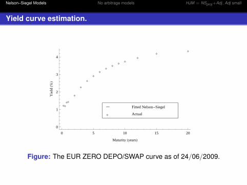
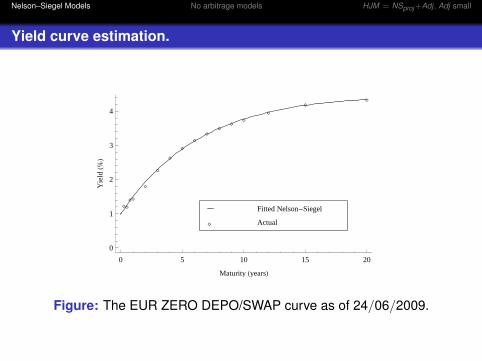
Figure: The EUR ZERO DEPO/SWAP curve as of 24/06/2009.
Nelson–Siegel Models No arbitrage models HJM = NSproj +Adj , Adj small
Yield curve estimation.
����
�
�
��
��
�� �
��
�
0 5 10 15 20
0
1
2
3
4
Maturity HyearsL
Yie
ldH%
L
� Actual
Fitted Nelson-Siegel
Figure: The EUR ZERO DEPO/SWAP curve as of 24/06/2009.
Nelson–Siegel Models No arbitrage models HJM = NSproj +Adj , Adj small
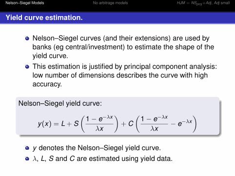
Yield curve estimation.
Nelson–Siegel curves (and their extensions) are used bybanks (eg central/investment) to estimate the shape of theyield curve.This estimation is justified by principal component analysis:low number of dimensions describes the curve with highaccuracy.
Nelson–Siegel yield curve:
y(x) = L + S(
1− e−λx
λx
)+ C
(1− e−λx
λx− e−λx
)
y denotes the Nelson–Siegel yield curve.λ, L, S and C are estimated using yield data.
Nelson–Siegel Models No arbitrage models HJM = NSproj +Adj , Adj small
Yield curve estimation.
5 10 15 20 25 30Maturity HyearsL
1%
2%
3%
4%
5%
YieldShocking the level.
L - 25 % L
L + 25 % L
L = 4.59
Increasing L
Decreasing L
5 10 15 20 25 30Maturity HyearsL
-4%
-3%
-2%
-1%
1%
2%
3%
4%
5%
6%
YieldShocking the slope.
S+150 % SS-150 % SS = -3.34
Negative S
Positive S
5 10 15 20 25 30Maturity HyearsL
1%
2%
3%
4%
YieldShocking the curvature.
C + 300 % C
C - 300 % C
C = -2.13Negative C
Positive C
Figure: Influence of shocks on the factor loadings of theNelson–Siegel yield curve.
Nelson–Siegel Models No arbitrage models HJM = NSproj +Adj , Adj small
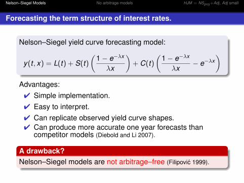
Forecasting the term structure of interest rates.
Nelson–Siegel yield curve forecasting model:
y(t , x) = L(t) + S(t)(
1− e−λx
λx
)+ C(t)
(1− e−λx
λx− e−λx
)Advantages:
4 Simple implementation.4 Easy to interpret.4 Can replicate observed yield curve shapes.4 Can produce more accurate one year forecasts than
competitor models (Diebold and Li 2007).
A drawback?Nelson–Siegel models are not arbitrage–free (Filipovic 1999).
Nelson–Siegel Models No arbitrage models HJM = NSproj +Adj , Adj small
No arbitrage models
§2 No arbitrage interest rate models:Heath–Jarrow–Morton.
Nelson–Siegel Models No arbitrage models HJM = NSproj +Adj , Adj small
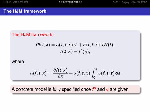
The HJM framework
The HJM framework:
df (t , x) = α(f , t , x) dt + σ(f , t , x) dW (t),f (0, x) = f o(x),
where
α(f , t , x) =∂f (t , x)
∂x+ σ(f , t , x)
∫ x
0σ(f , t , s) ds
A concrete model is fully specified once f o and σ are given.
Nelson–Siegel Models No arbitrage models HJM = NSproj +Adj , Adj small
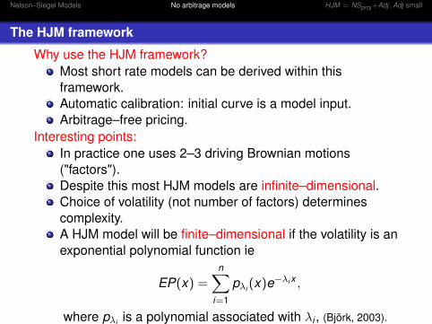
The HJM framework
Why use the HJM framework?Most short rate models can be derived within thisframework.Automatic calibration: initial curve is a model input.Arbitrage–free pricing.
Interesting points:In practice one uses 2–3 driving Brownian motions("factors").Despite this most HJM models are infinite–dimensional.Choice of volatility (not number of factors) determinescomplexity.A HJM model will be finite–dimensional if the volatility is anexponential polynomial function ie
EP(x) =n∑
i=1
pλi (x)e−λi x ,
where pλi is a polynomial associated with λi , (Björk, 2003).
Nelson–Siegel Models No arbitrage models HJM = NSproj +Adj , Adj small
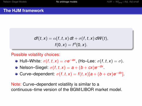
The HJM framework
df (t , x) = α(f , t , x) dt + σ(f , t , x) dW (t),f (0, x) = f o(0, x).
Possible volatility choices:Hull–White: σ(f , t , x) = σe−ax , (Ho–Lee: σ(f , t , x) = σ).Nelson–Siegel: σ(f , t , x) = a + (b + cx)e−dx .Curve–dependent: σ(f , t , x) = f (t , x)[a + (b + cx)e−dx ].
Note: Curve–dependent volatility is similar to acontinuous–time version of the BGM/LIBOR market model.
Nelson–Siegel Models No arbitrage models HJM = NSproj +Adj , Adj small
Research contribution
§3a Theoretical Contribution: HJM = NS+ Adj = NSproj+Adj
Nelson–Siegel Models No arbitrage models HJM = NSproj +Adj , Adj small
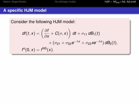
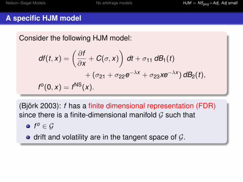
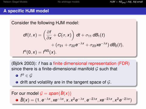
A specific HJM model
Consider the following HJM model:
df (t , x) =
(∂f∂x
+ C(σ, x)
)dt + σ11 dB1(t)
+ (σ21 + σ22e−λx + σ23xe−λx ) dB2(t),
f o(0, x) = f NS(x).
(Björk 2003): f has a finite dimensional representation (FDR)since there is a finite-dimensional manifold G such that
f o ∈ Gdrift and volatility are in the tangent space of G.
For our model G = span{B(x)}B(x) = (1,e−λx , xe−λx , x , x2e−λx ,e−2λx , xe−2λx , x2e−2λx )
Nelson–Siegel Models No arbitrage models HJM = NSproj +Adj , Adj small
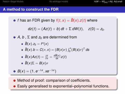
A method to construct the FDR
f has an FDR given by f (t , x) = B(x).z(t) where
dz(t) = (Az(t) + b) dt + Σ dW (t), z(0) = z0.
A, b , Σ and z0 are determined from
B(x).z0 = f o(x)
B(x).b = C(σ, x) = (B(x)σ)∫ x
0 (B(s)σ)T ds
B(x)Az(t) = ∂f∂x = dB(x)
dx z(t)
B(x)Σ = B(x)σ
B(x) = (1,e−λx , xe−λx )
Method of proof: comparison of coefficients.Easily generalised to exponential–polynomial functions.
Nelson–Siegel Models No arbitrage models HJM = NSproj +Adj , Adj small
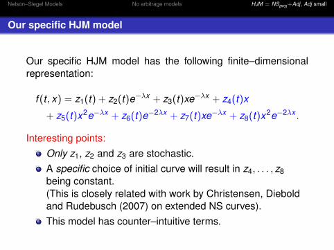
Our specific HJM model
Our specific HJM model has the following finite–dimensionalrepresentation:
f (t , x) = z1(t) + z2(t)e−λx + z3(t)xe−λx + z4(t)x
+ z5(t)x2e−λx + z6(t)e−2λx + z7(t)xe−λx + z8(t)x2e−2λx .
Interesting points:Only z1, z2 and z3 are stochastic.A specific choice of initial curve will result in z4, . . . , z8being constant.(This is closely related with work by Christensen, Dieboldand Rudebusch (2007) on extended NS curves).This model has counter–intuitive terms.
Nelson–Siegel Models No arbitrage models HJM = NSproj +Adj , Adj small
Our specific HJM model
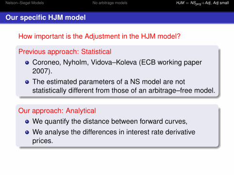
How important is the Adjustment in the HJM model?
Previous approach: StatisticalCoroneo, Nyholm, Vidova–Koleva (ECB working paper2007).The estimated parameters of a NS model are notstatistically different from those of an arbitrage–free model.
Our approach: AnalyticalWe quantify the distance between forward curves,We analyse the differences in interest rate derivativeprices.
Nelson–Siegel Models No arbitrage models HJM = NSproj +Adj , Adj small
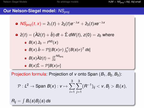
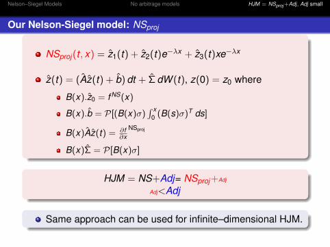
Our Nelson-Siegel model: NSproj
NSproj(t , x) = z1(t) + z2(t)e−λx + z3(t)xe−λx
z(t) = (Az(t) + b) dt + Σ dW (t), z(0) = z0 where
B(x).z0 = f NS(x)
B(x).b = P[(B(x)σ)∫ x
0 (B(s)σ)T ds]
B(x)Az(t) = ∂f∂x
NSproj
B(x)Σ = P[B(x)σ]
Projection formula: Projection of v onto Span (B1,B2,B3):
P : L2 → Span B(x) : v 7→3∑
i=1
3∑j=1
(R−1)ij < v ,Bj > Bi(x),
Rij =∫
Bi(s)Bj(s) ds
Nelson–Siegel Models No arbitrage models HJM = NSproj +Adj , Adj small
Our Nelson-Siegel model: NSproj
NSproj(t , x) = z1(t) + z2(t)e−λx + z3(t)xe−λx
z(t) = (Az(t) + b) dt + Σ dW (t), z(0) = z0 where
B(x).z0 = f NS(x)
B(x).b = P[(B(x)σ)∫ x
0 (B(s)σ)T ds]
B(x)Az(t) = ∂f∂x
NSproj
B(x)Σ = P[B(x)σ]
HJM = NS+Adj= NSproj+Adj
Adj<Adj
Same approach can be used for infinite–dimensional HJM.
Nelson–Siegel Models No arbitrage models HJM = NSproj +Adj , Adj small
Research contribution
§3b Applied Contribution: HJM = NS+ Adj = NSproj+Adj
Adj<Adj , Adj is small.
Nelson–Siegel Models No arbitrage models HJM = NSproj +Adj , Adj small
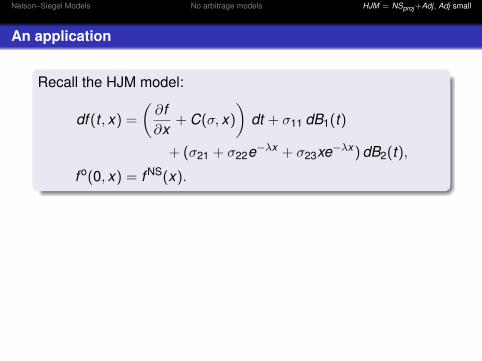
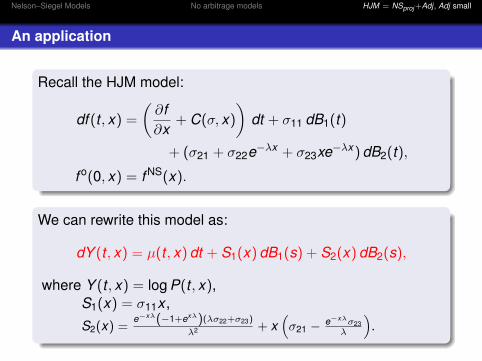
An application
Recall the HJM model:
df (t , x) =
(∂f∂x
+ C(σ, x)
)dt + σ11 dB1(t)
+ (σ21 + σ22e−λx + σ23xe−λx ) dB2(t),
f o(0, x) = f NS(x).
We can rewrite this model as:
dY (t , x) = µ(t , x) dt + S1(x) dB1(s) + S2(x) dB2(s),
where Y (t , x) = log P(t , x),S1(x) = σ11x ,S2(x) =
e−xλ(−1+exλ)(λσ22+σ23)
λ2 + x(σ21 − e−xλσ23
λ
).
Nelson–Siegel Models No arbitrage models HJM = NSproj +Adj , Adj small
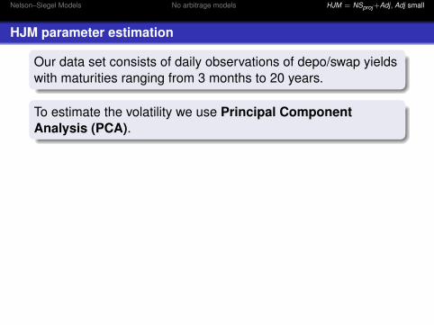
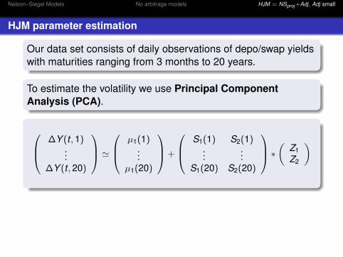
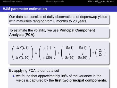
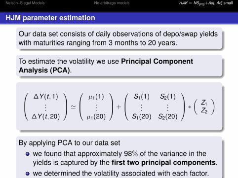
HJM parameter estimation
Our data set consists of daily observations of depo/swap yieldswith maturities ranging from 3 months to 20 years.
To estimate the volatility we use Principal ComponentAnalysis (PCA).
∆Y (t ,1)...
∆Y (t ,20)
' µ1(1)
...µ1(20)
+
S1(1) S2(1)...
...S1(20) S2(20)
∗ ( Z1Z2
)
By applying PCA to our data setwe found that approximately 98% of the variance in theyields is captured by the first two principal components.we determined the volatility associated with each factor.
Nelson–Siegel Models No arbitrage models HJM = NSproj +Adj , Adj small
HJM parameter estimation
Our data set consists of daily observations of depo/swap yieldswith maturities ranging from 3 months to 20 years.
To estimate the volatility we use Principal ComponentAnalysis (PCA).
∆Y (t ,1)...
∆Y (t ,20)
' µ1(1)
...µ1(20)
+
S1(1) S2(1)...
...S1(20) S2(20)
∗ ( Z1Z2
)
By applying PCA to our data setwe found that approximately 98% of the variance in theyields is captured by the first two principal components.
we determined the volatility associated with each factor.
Nelson–Siegel Models No arbitrage models HJM = NSproj +Adj , Adj small
HJM parameter estimation
Our data set consists of daily observations of depo/swap yieldswith maturities ranging from 3 months to 20 years.
To estimate the volatility we use Principal ComponentAnalysis (PCA).
∆Y (t ,1)...
∆Y (t ,20)
' µ1(1)
...µ1(20)
+
S1(1) S2(1)...
...S1(20) S2(20)
∗ ( Z1Z2
)
By applying PCA to our data setwe found that approximately 98% of the variance in theyields is captured by the first two principal components.we determined the volatility associated with each factor.
Nelson–Siegel Models No arbitrage models HJM = NSproj +Adj , Adj small
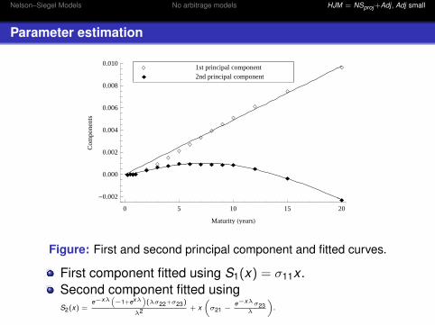
Parameter estimation
ííííí
í
í
í
í
í
í
í
í
í
í
í
ììììì
ì ìì ì ì ì ì ì
ì
ì
ì
0 5 10 15 20
-0.002
0.000
0.002
0.004
0.006
0.008
0.010
Maturity HyearsL
Com
pone
nts
ì 2nd principal componentí 1st principal component
Figure: First and second principal component and fitted curves.
First component fitted using S1(x) = σ11x .Second component fitted usingS2(x) =
e−xλ(−1+exλ
)(λσ22+σ23)
λ2 + x(σ21 − e−xλσ23
λ
).
Nelson–Siegel Models No arbitrage models HJM = NSproj +Adj , Adj small
Graphical analysis
0 5 10 15 200
1
2
3
4
5
6
7
Maturity HyearsL
Inst
anta
neou
sfo
rwar
dra
teH%
L
average NS
average HJM
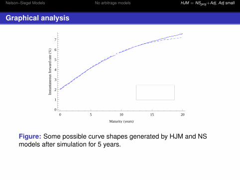
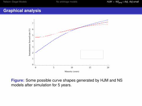
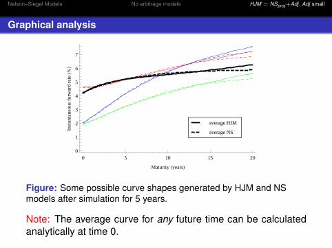
Figure: Some possible curve shapes generated by HJM and NSmodels after simulation for 5 years.
Nelson–Siegel Models No arbitrage models HJM = NSproj +Adj , Adj small
Graphical analysis
0 5 10 15 200
1
2
3
4
5
6
7
Maturity HyearsL
Inst
anta
neou
sfo
rwar
dra
teH%
L
average NS
average HJM
Figure: Some possible curve shapes generated by HJM and NSmodels after simulation for 5 years.

Nelson–Siegel Models No arbitrage models HJM = NSproj +Adj , Adj small
Graphical analysis
0 5 10 15 200
1
2
3
4
5
6
7
Maturity HyearsL
Inst
anta
neou
sfo
rwar
dra
teH%
L
average NS
average HJM
Figure: Some possible curve shapes generated by HJM and NSmodels after simulation for 5 years.
Nelson–Siegel Models No arbitrage models HJM = NSproj +Adj , Adj small
Graphical analysis
0 5 10 15 200
1
2
3
4
5
6
7
Maturity HyearsL
Inst
anta
neou
sfo
rwar
dra
teH%
L
average NS
average HJM
Figure: Some possible curve shapes generated by HJM and NSmodels after simulation for 5 years.
Note: The average curve for any future time can be calculatedanalytically at time 0.
Nelson–Siegel Models No arbitrage models HJM = NSproj +Adj , Adj small
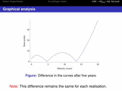
Graphical analysis
0 5 10 15 200
10
20
30
Maturity HyearsL
Bas
ispo
ints
Figure: Difference in the curves after five years.
Note: This difference remains the same for each realisation.
Nelson–Siegel Models No arbitrage models HJM = NSproj +Adj , Adj small
Analysis of simulated prices
Theoretical ‘European call option’ prices on a 20 year bond:
T0 (years) 5 10 15
Strike 0.565 0.686 0.865
ΠHJM(T0) 0.0193 0.0146 0.00567ΠNSproj (T0) 0.0192 0.0144 0.00562
% difference 0.47% 1.18% 0.89%
T0 denotes option maturity; Π denotes price.The strike is the at–the–money forward price of the bondP(T0,20− T0).
Nelson–Siegel Models No arbitrage models HJM = NSproj +Adj , Adj small
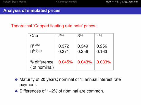
Analysis of simulated prices
Theoretical ‘Capped floating rate note’ prices:
Cap 2% 3% 4%
ΠHJM 0.372 0.349 0.256ΠNSproj 0.371 0.256 0.163
% difference 0.045% 0.043% 0.033%( of nominal)
Maturity of 20 years; nominal of 1; annual interest ratepayment.Differences of 1–2% of nominal are common.
Nelson–Siegel Models No arbitrage models HJM = NSproj +Adj , Adj small
Case Studies
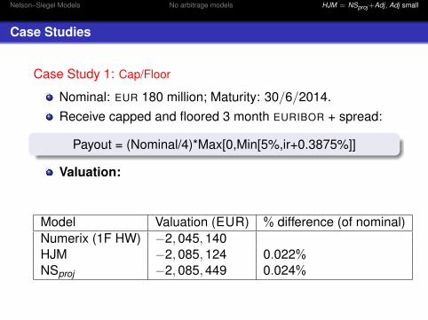
Case Study 1: Cap/Floor
Nominal: EUR 180 million; Maturity: 30/6/2014.Receive capped and floored 3 month EURIBOR + spread:
Payout = (Nominal/4)*Max[0,Min[5%,ir+0.3875%]]
Valuation:
Model Valuation (EUR) % difference (of nominal)Numerix (1F HW) −2,045,140HJM −2,085,124 0.022%NSproj −2,085,449 0.024%
Nelson–Siegel Models No arbitrage models HJM = NSproj +Adj , Adj small
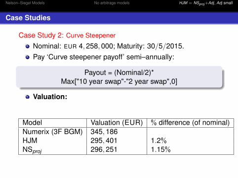
Case Studies
Case Study 2: Curve Steepener
Nominal: EUR 4,258,000; Maturity: 30/5/2015.Pay ‘Curve steepener payoff’ semi–annually:
Payout = (Nominal/2)*Max["10 year swap"-"2 year swap",0]
Valuation:
Model Valuation (EUR) % difference (of nominal)Numerix (3F BGM) 345,186HJM 295,401 1.2%NSproj 296,251 1.15%
Nelson–Siegel Models No arbitrage models HJM = NSproj +Adj , Adj small
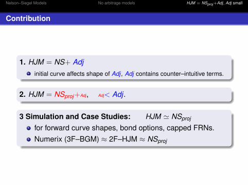
Contribution
1. HJM = NS+ Adjinitial curve affects shape of Adj , Adj contains counter–intuitive terms.
2. HJM = NSproj+Adj, Adj< Adj .
3 Simulation and Case Studies: HJM ' NSproj
for forward curve shapes, bond options, capped FRNs.Numerix (3F–BGM) ≈ 2F–HJM ≈ NSproj
Nelson–Siegel Models No arbitrage models HJM = NSproj +Adj , Adj small
Thank you
Research supported by:STAREBEI (Stages de Recherche á la BEI).The Embark Initiative operated by the Irish ResearchCouncil for Science, Technology and Engineering.The Edgeworth Centre for Financial Mathematics.
Disclaimer: This work expresses solely the views of the authorsand does not necessarily represent the opinion of the ECB orEIB.