Interest Rate Forecasts: A PathologyVol. 7 No. 2 Interest Rate Forecasts: A Pathology 139 Figure 3. RBNZ Interest Rate Forecast (Ninety Days, Annualized Rate) Published in Successive

Interest Rate Forecasts: A Pathology∗

Charles A. E. Goodhart and Wen Bin LimFinancial Markets Group

London School of Economics

This paper examines how well forecasters can predict thefuture time path of (policy-determined) short-term interestrates. Most prior work has been done using U.S. data; inthis exercise we use forecasts made for New Zealand by theReserve Bank of New Zealand (RBNZ) and those derived frommoney market yield curves in the United Kingdom. We broadlyreplicate recent U.S. findings for New Zealand and the UnitedKingdom, to show that such forecasts in New Zealand andthe United Kingdom have been excellent for the immediateforthcoming quarter, reasonable for the next quarter, and use-less thereafter. Moreover, when ex post errors are assesseddepending on whether interest rates have been in an upward,or downward, section of the cycle, they are shown to have beenbiased and, apparently, inefficient. We attempt to explain thosefindings, and examine whether the apparent ex post forecastinefficiencies may still be consistent with ex ante forecast effi-ciency. We conclude, first, that the best forecast may be ahybrid containing a specific forecast for the next six monthsand a “no-change” assumption thereafter, and, second, thatthe modal forecast for interest rates, and maybe for other vari-ables as well, is skewed, generally underestimating the likelycontinuation of the current phase of the cycle.

JEL Codes: C53, E17, E43, E47.

1. Introduction

The short-term policy interest rate has generally been adjusted inmost developed countries, at least during the last twenty years or so,in a series of small steps in the same direction, followed by a pause

∗Author contact: C.A.E. Goodhart, Financial Markets Group, Room R414,London School of Economics, Houghton Street, London WC2A 2AE, UnitedKingdom. E-mail: [email protected].

135

136 International Journal of Central Banking June 2011

Figure 1. Official Cash Rate: Reserve Bank ofNew Zealand

Source: Reserve Bank of New Zealand.

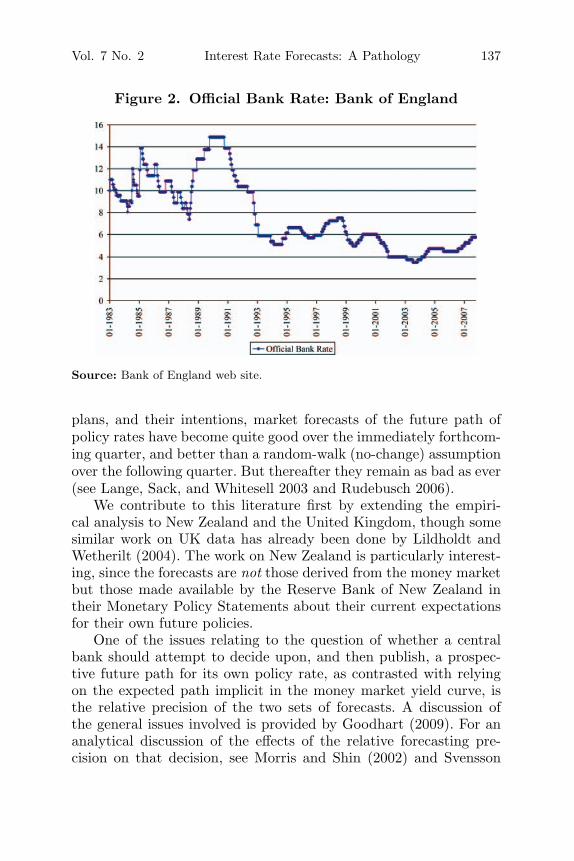
and then a, roughly, similar series of steps in the opposite direction.Figures 1 and 2 show the time path of policy rates for New Zealandand the United Kingdom, respectively.

On the face of it, such a behavioral pattern would appear quiteeasy to predict. Moreover, central bank behavior has typically beenmodeled by fitting a Taylor reaction function incorporating a laggeddependent variable with a large (often around 0.8 at a quarterly peri-odicity) and highly significant coefficient. But if this was, indeed, thereason for such gradualism, then the series of small steps should behighly predictable in advance.

The problem is that the evidence shows that they are not wellpredicted, beyond the next few months. There is a large body of,mainly American, literature to this effect, with the prime exponentbeing Glenn Rudebusch with a variety of co-authors; see in particularRudebusch (1995, 2002, and 2006). Indeed, prior to the mid-1990s,there is some evidence that the market could hardly predict thelikely path, or direction of movement, of policy rates over the nextfew months in the United States (see Rudebusch 1995 and 2002and the literature cited there). More recently, with central bankshaving become much more transparent about their thinking, their

Vol. 7 No. 2 Interest Rate Forecasts: A Pathology 137

Figure 2. Official Bank Rate: Bank of England

Source: Bank of England web site.

plans, and their intentions, market forecasts of the future path ofpolicy rates have become quite good over the immediately forthcom-ing quarter, and better than a random-walk (no-change) assumptionover the following quarter. But thereafter they remain as bad as ever(see Lange, Sack, and Whitesell 2003 and Rudebusch 2006).

We contribute to this literature first by extending the empiri-cal analysis to New Zealand and the United Kingdom, though somesimilar work on UK data has already been done by Lildholdt andWetherilt (2004). The work on New Zealand is particularly interest-ing, since the forecasts are not those derived from the money marketbut those made available by the Reserve Bank of New Zealand intheir Monetary Policy Statements about their current expectationsfor their own future policies.

One of the issues relating to the question of whether a centralbank should attempt to decide upon, and then publish, a prospec-tive future path for its own policy rate, as contrasted with relyingon the expected path implicit in the money market yield curve, isthe relative precision of the two sets of forecasts. A discussion ofthe general issues involved is provided by Goodhart (2009). For ananalytical discussion of the effects of the relative forecasting pre-cision on that decision, see Morris and Shin (2002) and Svensson


(2006). An assessment of the effects of publicly announcing the fore-cast on market rates is given in Andersson and Hofmann (2009) andin Ferrero and Nobili (2009).

The question of the likely precision of a central bank’s forecastof its own short-run policy rate is, however, at least in some largepart, empirical. The Reserve Bank of New Zealand (RBNZ), a serialinnovator in so many aspects of central banking, including inflationtargeting and the transparency (plus sanctions) approach to bankregulation, was, once again, the first to provide a forecast of the(conditional) path of its own future policy rates. It began to doso in 2000:Q1. That gives twenty-eight observations between thatdate and 2006:Q4, our sample period. While still short, this is nowlong enough to undertake some preliminary tests to examine forecastprecision.

Partly for the sake of comparison,1 we also explore the accuracyof the implicit market forecasts of the path of future short-terminterest rates in the United Kingdom. We use estimates provided bythe Bank of England over the period 1992:Q4 until 2004:Q4. Thereare two such series, one derived from the London Interbank OfferedRate (LIBOR) yield curve and one from short-dated governmentdebt. We base our choice between these on the relative accuracy oftheir forecasts. On this basis, as described in section 3, we chose,and subsequently used, the government debt series and its impliedforecasts.

In the next section, section 2, we report and describe our dataseries. Then in section 3 of this paper we examine the predictiveaccuracy of these sets of interest rate forecasts. The results areclosely in accord with the earlier findings in the United States.

1The United Kingdom and New Zealand (NZ) are different economies, andso one is not strictly comparing like with like. If one was, however, to comparethe NZ implicit market forecast accuracy with that of the RBNZ forecast overthe same period (a comparison which we hope that the RBNZ will do), the for-mer will obviously be affected by the latter (and possibly vice versa). Again, if aresearcher was to compare the implied accuracy of the market forecast prior tothe introduction of the official forecast with the accuracy of the market/officialforecast after the RBNZ had started to publish (another exercise that we hopethat the RBNZ will undertake), then the NZ economy, their financial system, andthe economic context may have changed over time. So one can never compare animplicit market forecast with an official forecast for interest rates on an exactlylike-for-like basis. Be that as it may, we view the comparison of the RBNZ and theimplied UK interest rate forecasts as illustrative, and not definitive in any way.


Figure 3. RBNZ Interest Rate Forecast (Ninety Days,Annualized Rate) Published in Successive Monetary

Policy Statements

Notes: Turning points are marked by a diamond. The dating of these is discussedfurther in section 3.

Whether the forecast comes from the central bank or from the mar-ket, the predictive ability is good, by most econometric standards,over the first quarter following the date of the forecast; it is poor, butsignificantly better than a no-change, random-walk forecast, over thesecond quarter (from end-month 3 to end-month 6), and effectivelyuseless from that horizon onward.

Worse, however, is to come. The forecasts, once beyond the endof the first quarter, are not only without value, they are, when com-pared with ex post outcomes, also strongly and significantly biased.This does not, however, necessarily mean that the forecasts were exante inefficient. We shall demonstrate in section 5 how ex post biascan yet be consistent with ex ante efficiency in forecasting.

This bias can actually be seen clearly in a visual representation ofthe forecasts. The RBNZ forecasts and outcome are shown in figure3, and the UK forecast derived from the short-dated governmentdebt yield curve and outcome is shown in figure 4.

What is apparent by simple inspection is that when interest ratesare on an upward (downward) cyclical path, the forecast underesti-mates (overestimates) the actual subsequent path of interest rates.Much the same pattern is also observable in the United States (see


Figure 4. UK Interest Rate Forecast (Ninety Days,Annualized Rate) Derived from the Short-Dated

Government Debt Yield Curve

Rudebusch 2007) and Sweden (see Adolfson et al. 2007). One of thereasons why this bias has not been more widely recognized up tillnow is that the biases during up and down cyclical periods are almostexactly offsetting, so if an econometrician applies his or her teststo the complete time series (as usual) (s)he will find no aggregatesign of bias. The distinction between the bias in “up” and “down”periods is crucial. A problem with some time series—e.g., those forinflation—is that the division of the sample into “up,” “down,” andin some cases “flat” periods is not always easy, nor self-evident. Butthis is less so for short-term interest rates where the ex post timingof turning points is relatively easier.

The sequencing of this paper proceeds as follows. We report ourdatabase in section 2. We examine the accuracy of the interest rateforecasts in section 3. We continue in section 4 by assessing whetherforecasts which appear ex post biased can still be ex ante efficient.Section 5 concludes.

2. The Database for Interest Rates

Our focus in this paper concerns the accuracy of forecasts for short-term policy-determined interest rates, measured in terms of unbi-asedness and the magnitude of forecast error. We examine the datafor two countries. We do so first for New Zealand, because this is the


country with the longest available published series of official projec-tions, as presented by the RBNZ in their quarterly Monetary PolicyStatement. Our second country is the United Kingdom. In this casethe Bank of England assumed unchanged future interests, from theircurrent level, as the basis of their forecasts, until they moved onto amarket-based estimate of future policy rates in November 2004. Asdescribed below, we considered the use of two alternative estimatesof future (forecast) policy rates.

In New Zealand, policy announcements, and the release of pro-jections, are usually made early in the final month of the calendarquarter, though the research work and discussions in their MonetaryPolicy Committee (MPC) will have mostly taken place a couple ofweeks previously. Thus the Statement contains a forecast for infla-tion for the current quarter (h = 0), though that will have been madewith knowledge of the outturn for the first month and some partialevidence for the second. The Policy Targets Agreement between theTreasurer and the Governor is specified in terms of the CPI, andthe forecast is made in terms of the CPI. This does not, however,mean that the RBNZ focuses exclusively on the overall CPI in itsassessment of inflationary pressures.

In New Zealand, the policy-determined rate is taken to be theninety-day (three-month) rate, and the forecasts are for that rate.Thus the current-quarter interest rate observation contains nearlytwo months of actual ninety-day rates and just over one month ofmarket forward one-month rates. If the MPC meeting results in a(revisable) decision to change interest rates in a way that is incon-sistent with the prediction that was previously embedded in marketforward interest rates, then the assumption for the current quartercan be revised to make the overall ninety-day track look consistentwith the policy message. Finally, the policy interest rate can beadjusted, after the forecast is effectively completed, right up to theday before the Monetary Policy Statement; this was done in Septem-ber 2001 after the terrorist attack. So, the interest rate forecast forthe current quarter (h = 0) also contains a small extent of uncertainforecast.

The data for published official forecasts of the policy rate startin 2000:Q1. We show those data, the forecasts, and the resultingerrors, for the policy rate in the appendix, tables 8 and 9. The dataare shown in a format where the forecasts are shown in the same


row as the actual to be forecast, so the forecast errors can be readoff directly.

The British case is somewhat more complicated. In the past,during the years of our sample, the MPC used a constant forwardforecast of the repo rate as the conditioning assumption for its fore-casting exercise. Whether members of the MPC made any mentalreservations about the forecast on account of a different subjectiveview about the future path of policy rates is an individual questionthat only they can answer personally. But it is hard to treat thatconstant path as a pure, most likely, forecast. At the same time,there are at least two alternative time series of implied market fore-casts for future policy rates that are derived from the yield curve ofshort-dated government debt and from LIBOR. There are some com-plicated technical issues in extracting implied forecasts from marketyield curves, and such yield curves can be distorted, especially theLIBOR yield curve, as experience since 2007 has clearly demon-strated. These problems relate largely to risk premia, notably creditand default risk; see Ferrero and Nobili (2009). The yield curve forgovernment debt is (or rather has been) largely immune to suchcredit (default) risk, though it can be exposed to other risks, e.g.,interest rate and liquidity risks.

We do not rehearse these difficulties here; instead we simplytook these data from the Bank of England web site (see www.bankofengland.co.uk). For more information on the procedures usedto obtain such implicit forecast series, see Anderson and Sleath(1999, 2001), Brooke, Cooper, and Scholtes (2000), and Joyce,Relleen, and Sorensen (2007). As will be reported in the next section,the government debt implicit market forecast series has had a moreaccurate forecast than the LIBOR series over our data period, 1992–2004, probably in part because the government series would nothave incorporated a time-varying credit risk element; see Ferrero andNobili (2009). Since the constant rate assumption was hardly a fore-cast, most of our work was done with the government debt implicitforecast series. This forecasts the three-month Treasury bill series.These series—actual, forecast, and errors (with the forecast lined upagainst the actual it was predicting)—are shown in the appendix,tables 10 and 11, for the government debt series (the other series forLIBOR is available from the authors on request).


3. How Accurate Are the Interest Rate Forecasts?

We began our examination of this question by running three regres-sions both for the NZ data series and for two sets of implied marketforecasts for the United Kingdom, derived from the LIBOR and gov-ernment debt yield curve, respectively. These regression equationswere as follows:

IR(t + h) = C1 + C2 Forecast (t, t + h) (1)

IR(t + h) − IR(t) = C1 + C2 [Forecast(t, t + h) − IR(t)](2)

IR(t + h) − IR(t + h − 1) = C1 + C2 [Forecast(t, t + h)

− Forecast(t, t + h − 1)], (3)

where

IR(t) = actual interest rate outturn at time t

Forecast(t, t + h) = forecast of IR(t + h) made at time t.

The first equation is essentially a Mincer-Zarnowitz regression(Mincer and Zarnowitz 1969) evaluating how well the forecast canpredict the actual h-period-ahead interest rate outturn (h = 0 ton). If the forecast perfectly matches the actual interest rate out-turn for every single period, we would expect to have C2 = 1 andC1 = 0. This can be seen as an evaluation of the bias of the fore-cast. Taking expectations on both sides, E{IR(t + h)} = E{C1 +C2[Forecast(t, t + h)}. A forecast is unbiased—i.e., E{IR(t + h)} =E{[Forecast(t, t + h)]} for all t—if and only if C2 = 1 and C1 = 0.The second regression, by subtracting the interest rate level fromboth sides, allows us to focus our attention on the performance ofthe forecast interest rate difference {IR(t + h) − IR(t)}. It asks, ash increases, how accurately can the forecaster forecast h-quarter-ahead interest rate changes from the present level. The third regres-sion is a slight twist on the second, focusing on one-period-aheadforecasts; the regression examines the forecast performance of one-period-ahead interest rate changes {IR(t + h) − IR(t + h − 1)} as hincreases.


All three regressions assess the accuracy/biasness of interest rateforecasts from slightly different angles. An unbiased forecast nec-essarily implies a constant term of zero and a slope coefficient ofone. We can test whether these conditions are fulfilled with a jointhypothesis test:

H0: C1 = 0 and C2 = 1.

With three equations, three data sets, and h = 0 to 5 for NewZealand and h = 1 to 8 for the UK series, we have some eighty-fiveregression results and statistical test scores to report.

We found that the regression results, estimated by OLS, for theimplicit forecasts derived from the LIBOR yield curve were compre-hensively worse than those from the government yield curve, or theRBNZ. These LIBOR results provided poor forecasts even for thefirst two quarters, and useless forecasts thereafter. There are severalpossible reasons for such worse forecasts—e.g., time-varying risk pre-mia (Ferrero and Nobili 2009) or data errors in a short sample—butit is beyond the scope of this paper to try to track them down. Theseresults can be found in Goodhart and Lim (2008) and, to save space,are not reported here. That reduces the number of regression resultsto sixteen in table 1 for the RBNZ and twenty-four in table 2 for theUK government yield curve.

These results show that the RBNZ forecast is excellent one quar-ter ahead but then becomes useless in forecasting the subsequentdirection, or extent, of change. Thus the coefficient C2 in equation(3) becomes −0.04 at h = 2 (with an R-squared of zero), and neg-ative thereafter. When the equation is run in levels, rather thanfirst differences—i.e., equation (1)—the excellent first-quarter fore-cast feeds through into a significantly positive forecast of the levelin the next few quarters, though it is just the first-quarter forecastdoing all the work. The Mincer-Zarnowitz test results2 are also con-sistent with our findings. We failed to reject the joint hypothesis H0for up to a three-quarters-ahead forecast for equation (1) and up toa four-quarters-ahead forecast for equation (2). We reject H0 for thequarters thereafter.

2These tests are reported in Goodhart and Lim (2008) but are omitted to savespace here.


Table 1. Regression Results for New Zealand

C1 C2

h = (p-value) (p-value) R-squared DW

Equation (1)

0 −0.01 1.00 0.99 1.77(0.93) (0.85)

1 −0.24 1.03 0.88 1.53(0.64) (0.74)

2 0.30 0.93 0.65 0.93(0.75) (0.63)

3 1.50 0.74 0.39 0.34(0.25) (0.19)

4 3.71 0.40 0.11 0.28(0.03) (0.02)

5 5.71 0.09 0.00 0.15(0.00) (0.00)

Equation (2)

1 −0.16 1.61 0.35 1.61(0.07) (0.18)

2 −0.15 1.02 0.20 1.02(0.31) (0.95)

3 −0.09 0.73 0.10 0.45(0.66) (0.55)

4 0.13 0.11 0.00 0.47(0.61) (0.10)

5 0.37 −0.38 0.03 0.34(0.20) (0.01)

Equation (3)

1 0.13 1.30 0.43 2.06(0.07) (0.33)

2 0.04 −0.04 0.00 1.24(0.65) (0.06)

3 0.07 −0.68 0.03 1.38(0.38) (0.04)

4 0.09 −1.29 0.07 1.37(0.28) (0.03)

5 0.09 −1.30 0.08 1.28(0.26) (0.02)

Note: The corresponding p-value is evaluated against the null hypothesis,H0: C1 = 0, C2 = 1.


Table 2. UK Forecasts Derived from the Short-TermGovernment Yield Curve

C1 C2


Equation (1)

1 0.23 0.98 0.95 1.94(0.25) (0.64)

2 0.60 0.89 0.84 1.03(0.07) (0.06)

3 0.98 0.79 0.71 0.62(0.03) (0.01)

4 1.56 0.67 0.55 0.43(0.00) (0.00)

5 2.10 0.56 0.41 0.35(0.00) (0.00)

6 2.43 0.49 0.34 0.31(0.00) (0.00)

7 2.52 0.47 0.32 0.29(0.00) (0.00)

8 2.42 0.48 0.35 0.28(0.00) (0.00)

Equation (2)

1 0.13 0.94 0.51 1.91(0.02) (0.70)

2 −0.01 0.86 0.50 1.04(0.84) (0.31)

3 −0.16 0.85 0.47 0.67(0.09) (0.25)

4 −0.28 0.73 0.36 0.48(0.03) (0.07)

5 −0.34 0.60 0.27 0.39(0.03) (0.01)

6 −0.37 0.51 0.22 0.35(0.03) (0.00)

7 −0.39 0.46 0.21 0.31(0.02) (0.00)

8 −0.43 0.46 0.24 0.28(0.00) (0.00)

(continued)


Table 2. (Continued)

C1 C2


Equation (3)

1 0.13 0.94 0.51 1.91(0.02) (0.70)

2 −0.13 0.87 0.25 1.19(0.02) (0.62)

3 −0.13 0.65 0.15 0.97(0.04) (0.14)

4 −0.09 0.43 0.05 0.83(0.19) (0.03)

5 −0.08 0.53 0.06 0.84(0.21) (0.14)

6 −0.08 0.73 0.08 0.80(0.18) (0.15)

7 −0.06 0.41 0.04 0.82(0.34) (0.58)

8 −0.05 0.58 0.03 0.76(0.39) (0.41)

Note: The corresponding p-value is evaluated against the null hypothesis, H0:C1 = 0, C2 = 1.

Turning next to the United Kingdom implied forecasts from thegovernment debt yield curve, what these tables indicate is that, inthe first quarter after the forecast is made, the forecast precisionof this derived forecast is mediocre (joint test for null hypothe-sis is rejected for h = 3 − 8), certainly significantly better thanrandom walk (no change) but not nearly as good as the NZ fore-cast over its first quarter. However, this market-based forecast isalso able to make a good forecast of the change in rates betweenQ1 and Q2 (whereas the RBNZ could not do that). The govern-ment yield forecast for h = 2 in table 2 is somewhat better thanfor h = 1. So the ability of the government yield forecast to pre-dict the level of the policy rate two quarters (six months) henceis about the same or a little better than that of the RBNZ. There-after, from Q2 onward, the predictive ability of the government yield


Figure 5. Stylized Pattern of Relationships betweenForecasts and Outturns of Macro Variables over the Cycle

forecast becomes insignificantly different from zero, but at least thecoefficients have the right sign (unlike the RBNZ).

The conclusion of this set of tests is that the precision of inter-est forecasts beyond the next quarter or two is approximately zero,whether they are made by the RBNZ or the UK market. Given thegradual adjustments in actual policy rates, this might seem surpris-ing. Why does it happen? In order to answer this question, we startwith a stylized fact. When one looks at most macroeconomic fore-casts, and notably so for interest rates (see figures 3 and 4 above),they tend to follow a pattern. When the macro variable is rising,the forecast increasingly falls below it. When the macro variable isfalling, the forecast increasingly lies above it. This pattern is shownagain in illustrative form in figure 5.

So, if we divide the sample period into periods of rising andfalling values for the variable of concern (in this case the interestrate), during up periods Actual minus Forecast will tend to be per-sistently positive, and during down periods Actual minus Forecastwill tend to be persistently negative. There is, however, an impor-tant caveat. A forecast made during an up (down) period may extendseveral quarters beyond the turning point into the next down (up)period. Once a turning point has occurred, however, a forecast thatwas too high (low) during the continuing down (up) cycle can rapidlythen become too low (high) once the cycle has switched direction.Clearly the tendency for Actual minus Forecast to be negative inan upturn will be most marked for forecasts made in an upturn solong as that upturn continues, i.e., until the next sign change from


up to down, or vice versa. Nevertheless, we still expect on balancethat forecasts made during an upturn (downturn) will tend to havepositive (negative) Actual minus Forecast outturns even after sucha sign change, but the result is clearly uncertain.3 But the forecastsmade for the policy rate in the next quarter (and to a lesser extentinto the second quarter) are so good, especially for the next quarterfor the RBNZ, that no such bias may exist.

As can be seen from figures 1 and 2, the official rate is frequentlyheld constant for a period of a few months before there is a reversalof direction. So the exact date of reversal is somewhat uncertain.We chose a date during these months as the best alternative on thebasis of other available contemporaneous evidence, notably the con-current time path of market rates. But we also tested for robustnessby taking the first and last dates of each flat period and rerunningthe exercises. The latter made no difference; the results are availableon request from the authors.

Perhaps the easiest way of demonstrating this result, suggestedto us by Andrew Patton, is to run a regression of the forecast error, atvarious horizons, against two indicator variables, one for up periods(C1) and one for down periods (C2):4

[IR(t + h) − Forecast(t, t + h)] = C1Iup(t + h) + C2Idown(t + h),(4)

where


Forecast(t, t + h) = forecast of IR(t + h) made at time t

Iup(t + h) is a dummy variable = 1 if time, t + h,

is an “up” period; else 0

Idown(t + h) is a dummy variable = 1 if time, t + h,

is a “down” period; else 0.

3When interest rates are volatile, and sign changes are more frequent, nothinguseful can be said about the likely outcomes of Actual minus Forecast after asecond sign change.

4In our original paper (Goodhart and Lim 2008), we did some additional andmore complicated statistical exercises, looking at the number of errors of a par-ticular sign, in “up” and “down” phases, their mean, standard deviation, andp-values. They are omitted here to save space.


Table 3. Results for New Zealand

A. Indicator Variable Is Based on State in NZ atOutturn Date (Whole Data Set)

H = Adj. R-sqr. C1 p-value C2 p-value

Q1 0.41 0.06 0.26 −0.34 0.00Q2 0.61 0.14 0.07 −0.69 0.00Q3 0.58 0.23 0.06 −0.88 0.00Q4 0.36 0.23 0.23 −0.99 0.00Q5 0.27 0.24 0.33 −1.06 0.01Q6 0.20 0.23 0.49 −1.07 0.05Q7 0.03 0.13 0.79 −0.95 0.27Q8 −0.30 0.04 0.97 −0.52 0.79

B. Indicator Variable Is Based on State in NZ atOutturn Date, but only Includes Period during

Which Sign Is Unchanged


Q1 0.41 0.06 0.26 −0.34 0.00Q2 0.76 0.22 0.00 −0.70 0.00Q3 0.87 0.41 0.00 −1.13 0.00Q4 0.81 0.56 0.00 −1.53 0.00Q5 0.86 0.73 0.00 −2.13 0.00Q6 — — — — —Q7 — — — — —Q8 — — — — —

Note: The corresponding p-value is evaluated against the null hypothesis, H0:C1 = 0, C2 = 0.

The hypothesis is that the up-period indicator (C1) is positive(actual > forecast) and the down-period indicator (C2) is negative(actual < forecast).

The results for New Zealand are shown in table 3.Turning next to the results for the UK government yield implied

forecasts, we found similar results. In this case, however, theforecasts included some sizable average errors, whereby the fore-casts implied that interest rates would tend to become higher thanwas the case in the historical event (actual < forecast). This average


Figure 6. Average UK Interest Rate Forecast Error

error tended to increase, approximately linearly, as the horizon (h)increased. This is shown in figure 6.

After correcting for this average error5 and rerunning,6 theresults were as shown in table 4.

One of our referees kindly directed our attention to a relatedrecent article, Ferrero and Nobili (2009). In this they regress excessreturns (x), defined as forecast less actual ex post outcomes, forinterest rates (futures) as a function of a business-cycle indicator(growth of output or employment expectations) and the current levelof the futures rate, so that in their equation (4), p. 116,

x(n)t+n = a(n) + βnzt + γnf

(n)t + ε

(n)t+n,

where zt is the business-cycle indicator, ft is the level of the currentfutures rate, and β and γ are coefficients. In their table 2 (p. 118),table 5 (p. 127), and table 7 (p. 131), they find β to be negative,often significantly so, and γ to be usually significantly positive.

These authors cannot explain their own findings: “A theoreticalanalysis of the reasons behind the presence of forecast errors thatare predictable and significantly countercyclical only in the United

5The tables using the unadjusted data—i.e., without correcting for the averageerror—are available on request from the authors.

6The average forecast error in New Zealand was much smaller and did notvary systematically with h. We ran similar adjusted regressions for New Zealand,but the results were closely similar to those shown in table 4.


Table 4. Results for United Kingdom, with AverageError Removed

A. Indicator Variable Is Based on State in UK atOutturn Date (Whole Data Set, with Average

Forecast Error Removed)


Q1 0.14 0.12 0.10 −0.08 0.16Q2 0.25 0.26 0.01 −0.19 0.02Q3 0.41 0.45 0.00 −0.38 0.00Q4 0.22 0.41 0.02 −0.39 0.02Q5 0.07 0.27 0.24 −0.30 0.17Q6 0.01 0.04 0.89 −0.13 0.60Q7 0.00 −0.19 0.50 −0.03 0.91Q8 0.03 −0.40 0.16 0.01 0.97

B. Indicator Variable Is Based on State in UK atOutturn Date, but only Includes Period during Which Sign

Is Unchanged, with Average Forecast Error Removed


Q1 0.14 0.12 0.10 −0.08 0.16Q2 0.32 0.28 0.01 −0.25 0.00Q3 0.63 0.57 0.00 −0.55 0.00Q4 0.70 0.79 0.00 −0.72 0.00Q5 0.76 0.85 0.00 −0.88 0.00Q6 0.81 0.76 0.00 −0.80 0.00Q7 0.76 0.76 0.03 −0.89 0.00Q8 0.67 0.52 0.23 −0.95 0.00

States lies beyond the scope of this paper” (Ferrero and Nobili 2009,p. 130). Our analysis here enables us to explain these findings; theyare exactly what we would have expected given the ex post biasesin forecasting over the cycle phases. As shown illustratively in figure5, during the up (down) phases of the cycle, forecasts understate(overstate) ex post actuals systematically; hence β will be negative,though we too cannot explain why the euro zone exhibits less of thiseffect. Similarly, the expected futures rate will tend to be highest(lowest) at the top (bottom) of the cycle. As figure 5 again shows,this is when the forecast bias has forecast greater (less) than actual,so γ should be positive. The explanation of the Ferrero/Nobili resultsis, in our view, not due to time-varying risk premia, but to system-atic ex post biases in the forecasting process over cycle phases. We


are particularly grateful for having been given the chance to relateour work here to another strand in the literature.

What all these results show is as follows:

(i) The official and market forecasts of interest rates that wehave studied here have significant predictive power over thenext two quarters, but virtually none thereafter. When fore-cast precision is effectively zero, as after two quarters hence,it is perhaps best to acknowledge this, e.g., by the centralbank using either a “no-change” thereafter assumption, orthe implied market forecast, for the more distant forecasts.7

(ii) These interest rate forecasts are systematically biased, under-estimating future policy rates during upturns and overesti-mating them during downturns. We shall now proceed toexplore reasons why this might have been so in sections 4and 5.

4. Can One Forecast the Forecasters?

In the preceding sections, we have shown that interest rate forecastsin the United Kingdom and New Zealand during this time period sys-tematically underpredicted the time series during cyclical phases ofupward movement, and similarly overpredicted during downswings.

In this section we seek to address the question of why these(most?) forecasts exhibit this tendency.8 The answer that we pro-pose is that (most) macroeconomic variables are expected (by most

7The choice may depend on the confidence with which the official forecastershold their longer-dated forecasts. There is, however, a danger that the officialforecasters have excessive confidence in their own forecasting abilities and thatprivate-sector forecasters likewise place excessive weight on such official forecasts(Morris and Shin 2002). However, the finding by Ferrero and Secchi (2009) thatlong-term expectations on future interest rates react significantly only to short-term central bank interest rate forecasts, and not to their longer-term projections,suggests that market agents may well realize that such longer-term projectionsrarely contain any valuable information.

8In our original work we extended our research to cover inflation forecastsas well. These also exhibited the same syndrome. In order to save space andto enhance focus, we have, however, omitted those results from this paper. Amore extended version of this paper, which explores not only the (errors in the)inflation forecasts in New Zealand and the United Kingdom but also the rela-tionships between the errors in the inflation forecasts and those in the interestrate forecasts, is given in Goodhart and Lim (2009).


economists9) to revert to some longer-term equilibrium, ceterisparibus. Indeed, it is hard to see how forecasting could be donein the absence of a concept of (long-run) equilibrium. But at anyparticular point of time, macroeconomic variables will be subject tomomentum, whose current force is quite difficult to assess accuratelyand which will be subject to unforeseeable future shocks. Thus weposit that these (most) forecasts will be subject to two main ele-ments, an autoregressive component and a mean-reverting (back toequilibrium) component. Such a combination is bound to give usthe general pattern that we have found in practice. So long as thephase remains upward (downward), the mean-reverting element inthe forecast will tend to pull the forecast below (above) the actualtrack of the variable, but, of course, as the eventual turning pointdraws closer, it will predict far better than a pure autoregressiveforecast.

During the periods under examination, an inflation-targetingregime was in operation in both New Zealand and the UnitedKingdom, so the equilibrium to which the inflation rate would revertwould have been close to target, and about 21

2 percent above thatfor the nominal interest rate, assuming an equilibrium real interestrate of 21

2 percent. But for our purposes here, we do not assume toknow what the equilibrium interest rate is, and have simply takenthe arithmetic average of the study period as an estimation of the“mean-reverting” point.10 The nature of the autoregressive processfor each series, and the coefficients for combining the autoregres-sive and the mean-reverting components into an implied forecastare unknown and for determination. Initially we shall assume thatthe forecasters make an efficient, unbiased prediction of both factors.Thus we estimate for each series

IR(t + 1) − IR(t) = B1 ∗ [IR(t) − IR(t − 1)] + B2 ∗ [IR(t) − IR], (5)

9Not all economists have such expectations. A few, “heterodox,” economistschallenge whether equilibria necessarily exist, notably Paul Davidson and BasilMoore.

10We tested this by trying values of the mean-reverting point with +1 percentand −1 percent of the average, and it made no significant difference to the coef-ficients for B1 and B2, as well as for the results in table 6 and table 7. Theseresults are available on request from the authors.


Table 5. Estimated Coefficients

RegressionEquation (1) B1 B2 Statistics

Adj.Coef. t-stats p-value Coef. t-stats p-value R-sqr. SE Obs.

UK InterestRate 0.66 6.30 0.00 −0.09 −2.54 0.01 0.4175 0.2539 54

NZ InterestRate 0.49 4.90 0.00 −0.13 −3.58 0.00 0.3403 0.6326 66

Figure 7. NZ Interest Rate: Comparison betweenOutturn, Actual and Implied Forecast

where


IR = average interest rate outturn over the study period.

The estimated coefficients are shown in table 5, where B1 can beunderstood as the autoregressive coefficient, and B2 as the mean-reversion coefficient.

Now we have a simplified model of how forecasts are done. Thenext step is to compare it with the actual forecasts. We do this firstdiagrammatically. For illustration, we have provided the diagram-matical comparison for the period between 2000:Q1 and 2002:Q4.The diagrams, figure 7 for New Zealand and figure 8 for the United


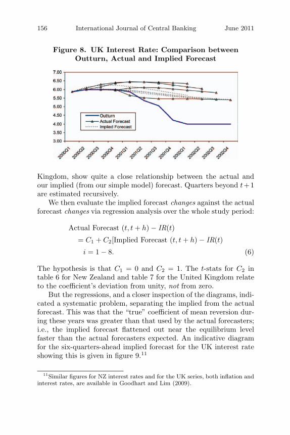
Figure 8. UK Interest Rate: Comparison betweenOutturn, Actual and Implied Forecast

Kingdom, show quite a close relationship between the actual andour implied (from our simple model) forecast. Quarters beyond t+1are estimated recursively.

We then evaluate the implied forecast changes against the actualforecast changes via regression analysis over the whole study period:

Actual Forecast (t, t + h) − IR(t)

= C1 + C2[Implied Forecast (t, t + h) − IR(t)

i = 1 − 8. (6)

The hypothesis is that C1 = 0 and C2 = 1. The t-stats for C2 intable 6 for New Zealand and table 7 for the United Kingdom relateto the coefficient’s deviation from unity, not from zero.

But the regressions, and a closer inspection of the diagrams, indi-cated a systematic problem, separating the implied from the actualforecast. This was that the “true” coefficient of mean reversion dur-ing these years was greater than that used by the actual forecasters;i.e., the implied forecast flattened out near the equilibrium levelfaster than the actual forecasters expected. An indicative diagramfor the six-quarters-ahead implied forecast for the UK interest rateshowing this is given in figure 9.11

11Similar figures for NZ interest rates and for the UK series, both inflation andinterest rates, are available in Goodhart and Lim (2009).


Table 6. NZ Interest Rate: Evaluation of Implied Forecastand Actual Forecast

C1 C2 Regression Statistics

Adj.h Coef. t-stats p-value Coef. t-stats p-value R-sqr. SE Obs.

1 0.05 1.76 0.09 0.48 −4.99 0.00 0.44 0.10 282 0.01 0.14 0.89 0.57 −3.87 0.00 0.48 0.17 283 −0.03 −0.41 0.69 0.52 −4.20 0.00 0.43 0.24 284 −0.04 −0.40 0.69 0.44 −4.95 0.00 0.35 0.30 285 −0.05 −0.44 0.66 0.40 −5.35 0.00 0.30 0.35 286 −0.13 −0.81 0.43 0.43 −4.36 0.00 0.33 0.38 217 −0.21 −1.02 0.33 0.48 −3.22 0.01 0.38 0.41 148 −0.31 −0.91 0.41 0.50 −2.12 0.09 0.36 0.48 7

Table 7. UK Interest Rate: Evaluation of ImpliedForecast and Actual Forecast

C1 C2 Regression Statistics

h Coef. t-stats p-value Coef. t-stats p-value R-sqr. SE Obs.

1 −0.16 −5.51 0.00 0.89 −0.93 0.36 0.65 0.17 342 −0.03 −0.49 0.63 0.81 −1.33 0.19 0.42 0.39 443 0.17 1.96 0.06 0.70 −1.84 0.07 0.28 0.59 474 0.31 2.82 0.01 0.59 −2.42 0.02 0.20 0.75 475 0.43 3.27 0.00 0.50 −2.92 0.01 0.14 0.89 476 0.51 3.52 0.00 0.44 −3.33 0.00 0.11 0.99 477 0.58 3.66 0.00 0.40 −3.64 0.00 0.09 1.07 478 0.63 3.74 0.00 0.37 −3.86 0.00 0.08 1.14 47

Incidentally, the implied forecasts often did better in predictingthe outturns than the actual forecasts. The results are available fromthe authors on request. This is not, however, so surprising since theimplied forecasts are obtained by finding the coefficients that bestexplained the ex post outturns, i.e., data mining. So we place noemphasis on this finding.

The actual forecasters placed less weight on mean reversion thanappeared to be the case in our constructed implied forecasts. That


Figure 9. UK Interest Rate, Six-Quarters-Ahead Forecast

forecasters should have underestimated the speed of reversion tothe mean is itself both plausible and understandable during theseyears. This was, after all, the period of the Great Moderation. Apossible definition of such a Great Moderation is a period when thekey macroeconomic time series revert to their (desired) equilibriumsomewhat faster than in the past or than currently expected.

Most macro variables are cyclical, but, as any forecaster knowsonly too well, it is extraordinarily difficult to predict turning points.Hence a forecast which combines a weighted average of autoregres-sive continuation and mean reversion is likely to be optimal. It shouldminimize the likelihood of a really big error, and will be unbiasedover the medium and longer run. So the behavior of the forecastersin seeking to estimate the likely mean outturn is, we would argue,appropriate.

Where our findings do indicate that there is a need for improve-ment is with the fan chart, or probability distribution, of futureoutcomes. This is usually shown as a symmetric single-peaked dis-tribution, often akin to a normal distribution with mode, mean, andmedian at the same point.

Our results show that this will generally not be the case. Themost probable outcome is that the cyclical phase will continue.Hence in an upturn (downturn), the most probable outcome is that(inflation and) interest rates will turn out to be systematically above(below) the mean forecast. But this is balanced by a smaller proba-bility that the cycle will turn within this interval. But if there shouldbe such a turning point, following an upturn (downturn) phase, then


the forecasts will considerably overstate (understate) the subsequentdownward (upward) movement.

5. Conclusions

In this paper we have demonstrated that, in the two countries andshort data periods studied, the forecasts of interest rates had littleor no informational value when the horizon exceeded two quarters(six months), though they were good in the next quarter and rea-sonable in the second quarter out. Moreover, all the forecasts wereex post and, systematically, inefficient, underestimating (overesti-mating) future outturns during up (down) cycle phases. The mainreason for this is that forecasters cannot predict the timing of cycli-cal turning points, and hence predict future developments as a con-vex combination of autoregressive momentum and a reversion toequilibrium.

There are, perhaps, two main conclusions that can be drawn fromthis. The first is that official interest rate forecasts should probablybe presented in hybrid form. MPCs and markets can make reason-able forecasts of interest rates up to two (at an extreme pinch,three) quarters hence. These should, indeed, be the basis of fore-casts. Beyond that horizon, they are rarely able to do so, and thattoo should be acknowledged. Unless the authorities have a particularreason for exhibiting confidence in their own longer-dated forecasts,those same (longer-dated) forecasts should be presented in a specif-ically formulaic manner, e.g., constant or based on implied forwardmarket rates.

The second conclusion is that the resulting interest (and infla-tion) forecast is generally not modal. It is biased, underestimating(overestimating) in upturns (downturns), because the forecaster isprotecting himself or herself against extreme errors by assuming a(roughly constant) small probability of a turning point in the cycleoccurring in each quarter. Consequently the most likely outturn inany expansionary phase is that output, inflation, and interest rateswill turn out above forecast (vice versa in a downturn). The con-clusion that we would draw from this is that policy needs to benormally somewhat more aggressive than the mean forecast wouldindicate (raising rates in booms, cutting rates in recessions), but thatthe policymakers need to be alert to (unpredictable) turning pointsand therefore to the occasional need to reverse course abruptly.


Appen

dix

Tab

le8.

RB

NZ

Inte

rest

Rat

eFor

ecas

t

Inte

rest

Dat

eR

ate

Sta

tea

r(t

,t)

r(t

−1,t)

r(t

−2,t)

r(t

−3,t)

r(t

−4,t)

r(t

−5,t)

r(t

−6,t)

r(t

−7,t)

r(t

−8,t)

2000

:Q1

5.97

15.

86N

/AN

/AN

/AN

/AN

/AN

/AN

/AN

/A20

00:Q

26.

731

6.46

6.21

N/A

N/A

N/A

N/A

N/A

N/A

N/A

2000

:Q3

6.74

16.

836.

846.

49N

/AN

/AN

/AN

/AN

/AN

/A20

00:Q

46.

67−

16.

646.

837.

156.

70N

/AN

/AN

/AN

/AN

/A20

01:Q

16.

42−

16.

506.

846.

917.

366.

88N

/AN

/AN

/AN

/A20

01:Q

25.

85−

15.

846.

317.

107.

017.

487.

05N

/AN

/AN

/A20

01:Q

35.

74−

15.

795.

836.

307.

167.

077.

537.

19N

/AN

/A20

01:Q

44.

97−

15.

075.

875.

816.

347.

267.

107.

537.

27N

/A20

02:Q

15.

031

4.91

5.18

5.90

5.74

6.38

7.38

7.13

7.51

7.28

2002

:Q2

5.82

15.

725.

415.

225.

925.

746.

39N

/AN

/AN

/A20

02:Q

35.

911

5.97

6.30

5.81

5.20

5.98

5.73

6.38

N/A

N/A

2002

:Q4

5.90

−1

6.00

6.16

6.70

6.08

5.14

6.10

5.76

6.36

N/A

2003

:Q1

5.83

−1

5.88

6.00

6.26

6.93

6.22

5.12

6.23

5.90

6.35

2003

:Q2

5.44

−1

5.47

5.88

6.00

6.27

7.03

6.34

N/A

N/A

N/A

2003

:Q3

5.12

−1

5.12

5.32

5.88

6.00

6.11

7.04

6.18

N/A

N/A

2003

:Q4

5.29

15.

325.

225.

315.

886.

005.

886.

875.

96N

/A20

04:Q

15.

491

5.51

5.54

5.28

5.31

5.88

6.00

5.69

6.72

5.79

2004

:Q2

5.86

15.

765.

675.

715.

315.

325.

88N

/AN

/AN

/A20

04:Q

36.

441

6.35

6.14

5.73

5.82

5.37

5.36

5.88

N/A

N/A

(con

tinu

ed)


Tab

le8.

(Con

tinued

)

Inte

rest

Dat

eR

ate

Sta

tea

r(t

,t)

r(t

−1,t)

r(t

−2,t)

r(t

−3,t)

r(t

−4,t)

r(t

−5,t)

r(t

−6,t)

r(t

−7,t)

r(t

−8,t)

2004

:Q4

6.73

16.

746.

616.

315.

755.

905.

475.

445.

88N

/A20

05:Q

16.

861

6.80

6.80

6.68

6.40

5.75

5.95

5.57

5.52

5.88

2005

:Q2

7.04

17.

007.

006.

836.

736.

455.

75N

/AN

/AN

/A20

05:Q

37.

051

7.05

7.12

7.07

6.82

6.76

6.49

5.77

N/A

N/A

2005

:Q4

7.49

17.

477.

217.

157.

076.

836.

786.

535.

81N

/A20

06:Q

17.

551

7.57

7.61

7.32

7.14

7.09

6.82

6.78

6.54

5.84

2006

:Q2

7.48

17.

497.

557.

597.

317.

157.

10N

/AN

/AN

/A20

06:Q

37.

511

7.48

7.55

7.56

7.58

7.30

7.16

7.09

N/A

N/A

2006

:Q4

7.64

17.

627.

627.

537.

537.

597.

297.

177.

09N

/A

a“+

1”in

dic

ates

an“u

p”

per

iod,i.e.

,a

per

iod

ofri

sing

inte

rest

rate

;“−

1”in

dic

ates

a“d

own”

per

iod,i.e.

,a

per

iod

ofdec

linin

gin

tere

stra

te.

Sourc

e:T

he

NZ

dat

aar

eta

ken

from

thei

rqu

arte

rly

Mon

etar

yPol

icy

Sta

tem

ents

.For

mor

edet

ail,

see

sect

ion

2.


Tab

le9.

RB

NZ

Inte

rest

Rat

eFor

ecas

tErr

or(T

able

Updat

ed)

For

ecas

tErr

orr(t

,t)

r(t

−1,

t)r(t

−2,

t)r(t

−3,

t)r(t

−4,

t)r(t

−5,

t)r(t

−6,

t)r(t

−7,

t)r(t

−8,

t)

2000

:Q1

0.11

N/A

N/A

N/A

N/A

N/A

N/A

N/A

N/A

2000

:Q2

0.27

0.52

N/A

N/A

N/A

N/A

N/A

N/A

N/A

2000

:Q3

−0.

09−

0.10

0.25

N/A

N/A

N/A

N/A

N/A

N/A

2000

:Q4

0.03

−0.

16−

0.48

−0.

03N

/AN

/AN

/AN

/AN

/A20

01:Q

1−

0.08

−0.

42−

0.49

−0.

94−

0.47

N/A

N/A

N/A

N/A

2001

:Q2

0.01

−0.

46−

1.25

−1.

16−

1.63

−1.

20N

/AN

/AN

/A20

01:Q

3−

0.05

−0.

09−

0.56

−1.

42−

1.33

−1.

79−

1.46

N/A

N/A

2001

:Q4

−0.

10−

0.90

−0.

84−

1.37

−2.

29−

2.13

−2.

56−

2.30

N/A

2002

:Q1

0.12

−0.

15−

0.87

−0.

70−

1.34

−2.

35−

2.10

−2.

48−

2.25

2002

:Q2

0.10

0.41

0.60

−0.

100.

08−

0.57

N/A

N/A

N/A

2002

:Q3

−0.

06−

0.38

0.10

0.72

−0.

070.

18−

0.47

N/A

N/A

2002

:Q4

−0.

10−

0.26

−0.

80−

0.18

0.75

−0.

210.

14−

0.47

N/A

2003

:Q1

−0.

05−

0.17

−0.

43−

1.11

−0.

390.

71−

0.41

−0.

07−

0.52

2003

:Q2

−0.

03−

0.44

−0.

56−

0.84

−1.

59−

0.90

N/A

N/A

N/A

2003

:Q3

0.00

−0.

20−

0.76

−0.

88−

0.98

−1.

91−

1.06

N/A

N/A

2003

:Q4

−0.

030.

07−

0.02

−0.

59−

0.71

−0.

59−

1.58

−0.

67N

/A20

04:Q

1−

0.02

−0.

050.

220.

19−

0.39

−0.

51−

0.20

−1.

23−

0.29

2004

:Q2

0.10

0.19

0.15

0.55

0.54

−0.

02N

/AN

/AN

/A

(con

tinu

ed)


Tab

le9.

(Con

tinued

)

For

ecas

tErr

orr(t

,t)

r(t

−1,

t)r(t

−2,

t)r(t

−3,

t)r(t

−4,

t)r(t

−5,

t)r(t

−6,

t)r(t

−7,

t)r(t

−8,

t)

2004

:Q3

0.09

0.30

0.71

0.62

1.07

1.08

0.56

N/A

N/A

2004

:Q4

−0.

010.

110.

410.

980.

821.

261.

290.

85N

/A20

05:Q

10.

060.

060.

180.

461.

110.

911.

291.

340.

9820

05:Q

20.

040.

050.

210.

310.

591.

29N

/AN

/AN

/A20

05:Q

30.

00−

0.07

−0.

020.

230.

290.

561.

28N

/AN

/A20

05:Q

40.

020.

290.

350.

420.

660.

710.

971.

68N

/A20

06:Q

1−

0.02

−0.

060.

230.

410.

460.

730.

771.

011.

7120

06:Q

2−

0.01

−0.

07−

0.11

0.17

0.32

0.38

N/A

N/A

N/A

2006

:Q3

0.03

−0.

04−

0.05

−0.

070.

210.

350.

42N

/AN

/A20

06:Q

40.

020.

030.

110.

110.

050.

360.

480.

56N

/A

Note

:E

rror

isA

ctua

lm

inus

Fore

cast

.


Tab

le10

.U

KIn

tere

stR

ate

For

ecas

tIm

plied

by

Gov

ernm

ent

Yie

ldC

urv

e

Inte

rest

Dat

eR

ate

Sta

tea

r(t

−1,t)

r(t

−2,t)

r(t

−3,t)

r(t

−4,t)

r(t

−5,t)

r(t

−6,t)

r(t

−7,t)

r(t

−8,t)

1993

:Q1

6.13

−1

N/A

N/A

N/A

N/A

N/A

N/A

N/A

N/A

1993

:Q2

5.88

−1

N/A

5.95

N/A

N/A

N/A

N/A

N/A

N/A

1993

:Q3

5.88

−1

N/A

5.22

6.18

N/A

N/A

N/A

N/A

N/A

1993

:Q4

5.66

−1

N/A

5.60

5.36

6.56

N/A

N/A

N/A

N/A

1994

:Q1

5.22

−1

N/A

5.12

6.02

5.66

6.85

N/A

N/A

N/A

1994

:Q2

5.13

1N

/A5.

145.

176.

435.

987.

07N

/AN

/A19

94:Q

35.

241

N/A

4.77

5.17

5.38

6.76

6.28

7.24

N/A

1994

:Q4

5.75

1N

/A5.

364.

945.

305.

657.

036.

567.

4019

95:Q

16.

451

N/A

6.55

6.08

5.21

5.49

5.92

7.26

6.81

1995

:Q2

6.63

−1

N/A

N/A

7.23

6.73

5.49

5.71

6.17

7.47

1995

:Q3

6.63

−1

N/A

7.14

7.42

7.80

7.27

5.75

5.93

6.40

1995

:Q4

6.58

−1

6.49

6.97

7.73

7.97

8.24

7.69

5.98

6.14

1996

:Q1

6.13

−1

N/A

6.76

7.39

8.20

8.39

8.57

8.01

6.18

1996

:Q2

5.87

−1

5.68

6.16

7.08

7.73

8.52

8.68

8.83

8.26

1996

:Q3

5.69

1N

/A5.

646.

297.

397.

958.

728.

889.

0219

96:Q

45.

861

5.60

N/A

5.84

6.50

7.63

8.09

8.85

9.00

1997

:Q1

5.94

1N

/A5.

746.

426.

126.

717.

828.

188.

9319

97:Q

26.

201

N/A

6.63

6.01

6.74

6.37

6.90

7.96

8.24

1997

:Q3

6.87

16.

22N

/A6.

886.

347.

016.

607.

068.

0619

97:Q

47.

151

6.87

6.51

6.43

7.04

6.62

7.24

6.80

7.19

1998

:Q1

7.25

17.

266.

956.

676.

577.

136.

867.

436.

97

(con

tinu

ed)


Tab

le10

.(C

ontinued

)

Inte

rest

Dat

eR

ate

Sta

tea

r(t

−1,t)

r(t

−2,t)

r(t

−3,t)

r(t

−4,t)

r(t

−5,t)

r(t

−6,t)

r(t

−7,t)

r(t

−8,t)

1998

:Q2

7.33

17.

007.

226.

996.

766.

667.

197.

047.

5819

98:Q

37.

50−

16.

946.

697.

106.

996.

806.

737.

237.

1919

98:Q

46.

86−

17.

216.

716.

517.

006.

986.

836.

787.

2519

99:Q

15.

69−

16.

106.

966.

536.

396.

936.

986.

856.

8219

99:Q

25.

20−

14.

805.

796.

696.

416.

306.

876.

986.

8719

99:Q

35.

071

4.89

4.69

5.51

6.46

6.31

6.21

6.82

6.98

1999

:Q4

5.40

14.

894.

894.

715.

286.

266.

216.

136.

7720

00:Q

15.

871

5.37

5.10

4.94

4.72

5.10

6.09

6.13

6.05

2000

:Q2

6.00

−1

6.07

5.79

5.45

5.02

4.70

4.96

5.93

6.05

2000

:Q3

6.00

−1

6.14

6.29

6.00

5.75

5.08

4.66

4.86

5.80

2000

:Q4

6.00

−1

5.95

6.36

6.40

6.09

5.93

5.11

4.61

4.77

2001

:Q1

5.86

−1

5.65

6.08

6.44

6.43

6.13

6.02

5.13

4.56

2001

:Q2

5.36

−1

5.34

5.52

6.12

6.43

6.43

6.13

6.06

5.13

2001

:Q3

5.05

−1

4.90

5.16

5.47

6.09

6.36

6.41

6.10

6.06

2001

:Q4

4.23

−1

4.66

4.89

5.14

5.46

6.03

6.26

6.38

6.05

2002

:Q1

4.00

−1

3.77

4.83

4.95

5.14

5.46

5.96

6.15

6.34

2002

:Q2

4.00

−1

4.01

3.92

5.01

5.02

5.15

5.44

5.89

6.04

2002

:Q3

4.00

−1

4.17

4.41

4.14

5.12

5.08

5.14

5.42

5.82

(con

tinu

ed)


Tab

le10

.(C

ontinued

)

Inte

rest

Dat

eR

ate

Sta

tea

r(t

−1,t)

r(t

−2,t)

r(t

−3,t)

r(t

−4,t)

r(t

−5,t)

r(t

−6,t)

r(t

−7,t)

r(t

−8,t)

2002

:Q4

4.00

−1

3.74

4.59

4.68

4.32

5.19

5.12

5.13

5.39

2003

:Q1

3.85

−1

3.72

3.80

4.90

4.85

4.47

5.22

5.14

5.12

2003

:Q2

3.75

−1

3.38

3.68

3.98

5.12

4.97

4.59

5.24

5.15

2003

:Q3

3.53

−1

3.34

3.27

3.76

4.19

5.27

5.04

4.69

5.24

2003

:Q4

3.65

13.

363.

273.

243.

894.

375.

375.

094.

7720

04:Q

13.

911

3.96

3.60

3.28

3.29

4.02

4.52

5.44

5.12

2004

:Q2

4.22

13.

954.

183.

843.

353.

384.

134.

645.

4920

04:Q

34.

651

4.42

4.10

4.35

4.03

3.44

3.49

4.24

4.73

2004

:Q4

4.75

14.

804.

684.

194.

494.

183.

543.

604.

33

a“+

1”in

dic

ates

an“u

p”

per

iod,i.e.

,a

per

iod

ofri

sing

inte

rest

rate

;“−

1”in

dic

ates

a“d

own”

per

iod,i.e.

,a

per

iod

ofdec

linin

gin

tere

stra

te.

Sourc

e:T

he

UK

dat

aar

eta

ken

from

the

Ban

kof

Engl

and

web

site

,w

ww

.ban

kofe

ngl

and.c

o.uk.

For

mor

edet

ail,

see

sect

ion

2.


Tab

le11

.Im

plied

Err

orfr

omU

KG

over

nm

ent

Yie

ldFor

ecas

t(T

able

Updat

ed)

For

ecas

tErr

orr(t

−1,

t)r(t

−2,

t)r(t

−3,

t)r(t

−4,

t)r(t

−5,

t)r(t

−6,

t)r(t

−7,

t)r(t

−8,

t)

1993

:Q1

N/A

N/A

N/A

N/A

N/A

N/A

N/A

N/A

1993

:Q2

N/A

N/A

−0.

07N

/AN

/AN

/AN

/AN

/A19

93:Q

3N

/AN

/A0.

66−

0.30

N/A

N/A

N/A

N/A

1993

:Q4

N/A

N/A

0.06

0.30

−0.

90N

/AN

/AN

/A19

94:Q

1N

/AN

/A0.

10−

0.80

−0.

44−

1.63

N/A

N/A

1994

:Q2

N/A

N/A

−0.

01−

0.04

−1.

30−

0.85

−1.

94N

/A19

94:Q

3N

/AN

/A0.

470.

07−

0.14

−1.

52−

1.04

−2.

0019

94:Q

4N

/AN

/A0.

390.

810.

450.

10−

1.28

−0.

8119

95:Q

1N

/AN

/A−

0.10

0.37

1.24

0.96

0.53

−0.

8119

95:Q

2N

/AN

/AN

/A−

0.60

−0.

101.

140.

920.

4619

95:Q

3N

/AN

/A−

0.51

−0.

79−

1.17

−0.

640.

880.

7019

95:Q

4N

/A0.

09−

0.39

−1.

15−

1.39

−1.

66−

1.11

0.60

1996

:Q1

N/A

N/A

−0.

63−

1.26

−2.

07−

2.26

−2.

44−

1.88

1996

:Q2

N/A

0.19

−0.

29−

1.21

−1.

86−

2.65

−2.

81−

2.96

1996

:Q3

N/A

N/A

0.05

−0.

60−

1.70

−2.

26−

3.03

−3.

1919

96:Q

4N

/A0.

26N

/A0.

02−

0.64

−1.

77−

2.23

−2.

9919

97:Q

1N

/AN

/A0.

20−

0.48

−0.

18−

0.77

−1.

88−

2.24

1997

:Q2

N/A

N/A

−0.

430.

19−

0.54

−0.

17−

0.70

−1.

7619

97:Q

3N

/A0.

65N

/A−

0.01

0.53

−0.

140.

27−

0.19

1997

:Q4

N/A

0.28

0.64

0.72

0.11

0.53

−0.

090.

3519

98:Q

1N

/A−

0.01

0.30

0.58

0.68

0.12

0.39

−0.

18

(con

tinu

ed)


Tab

le11

.(C

ontinued

)

For

ecas

tErr

orr(t

−1,

t)r(t

−2,

t)r(t

−3,

t)r(t

−4,

t)r(t

−5,

t)r(t

−6,

t)r(t

−7,

t)r(t

−8,

t)

1998

:Q2

N/A

0.33

0.11

0.34

0.57

0.67

0.14

0.29

1998

:Q3

N/A

0.56

0.81

0.40

0.51

0.70

0.77

0.27

1998

:Q4

N/A

−0.

350.

150.

35−

0.14

−0.

120.

030.

0819

99:Q

1N

/A−

0.41

−1.

27−

0.84

−0.

70−

1.24

−1.

29−

1.16

1999

:Q2

N/A

0.40

−0.

59−

1.49

−1.

21−

1.10

−1.

67−

1.78

1999

:Q3

N/A

0.18

0.38

−0.

44−

1.39

−1.

24−

1.14

−1.

7519

99:Q

4N

/A0.

510.

510.

690.

12−

0.86

−0.

81−

0.73

2000

:Q1

N/A

0.50

0.77

0.93

1.15

0.77

−0.

22−

0.26

2000

:Q2

N/A

−0.

070.

210.

550.

981.

301.

040.

0720

00:Q

3N

/A−

0.14

−0.

290.

000.

250.

921.

341.

1420

00:Q

4N

/A0.

05−

0.36

−0.

40−

0.09

0.07

0.89

1.39

2001

:Q1

N/A

0.21

−0.

22−

0.58

−0.

57−

0.27

−0.

160.

7320

01:Q

2N

/A0.

02−

0.16

−0.

76−

1.07

−1.

07−

0.77

−0.

7020

01:Q

3N

/A0.

15−

0.11

−0.

42−

1.04

−1.

31−

1.36

−1.

0520

01:Q

4N

/A−

0.43

−0.

66−

0.91

−1.

23−

1.80

−2.

03−

2.15

2002

:Q1

N/A

0.23

−0.

83−

0.95

−1.

14−

1.46

−1.

96−

2.15

(con

tinu

ed)


Tab

le11

.(C

ontinued

)

For

ecas

tErr

orr(t

−1,

t)r(t

−2,

t)r(t

−3,

t)r(t

−4,

t)r(t

−5,

t)r(t

−6,

t)r(t

−7,

t)r(t

−8,

t)

2002

:Q2

N/A

−0.

010.

08−

1.01

−1.

02−

1.15

−1.

44−

1.89

2002

:Q3

N/A

−0.

17−

0.41

−0.

14−

1.12

−1.

08−

1.14

−1.

4220

02:Q

4N

/A0.

26−

0.59

−0.

68−

0.32

−1.

19−

1.12

−1.

1320

03:Q

1N

/A0.

130.

05−

1.05

−1.

00−

0.62

−1.

37−

1.29

2003

:Q2

N/A

0.37

0.07

−0.

23−

1.37

−1.

22−

0.84

−1.

4920

03:Q

3N

/A0.

190.

26−

0.23

−0.

66−

1.74

−1.

51−

1.16

2003

:Q4

N/A

0.29

0.38

0.41

−0.

24−

0.72

−1.

72−

1.44

2004

:Q1

N/A

−0.

050.

310.

630.

62−

0.11

−0.

61−

1.53

2004

:Q2

N/A

0.27

0.04

0.38

0.87

0.84

0.09

−0.

4220

04:Q

3N

/A0.

230.

550.

300.

621.

211.

160.

4120

04:Q

4N

/A−

0.05

0.07

0.56

0.26

0.57

1.21

1.15

Note

:E

rror

isA

ctua

lm

inus

Fore

cast

.


References

Adolfson, M., M. K. Andersson, J. Linde, M. Villani, and A. Vredin.2007. “Modern Forecasting Models in Action: Improving Macro-economic Analyses at Central Banks.” International Journal ofCentral Banking 3 (4): 111–44.

Anderson, N., and J. Sleath. 1999. “New Estimates of the UK Realand Nominal Yield Curves.” Quarterly Bulletin (Bank of Eng-land) (November): 384–92.

———. 2001. “New Estimates of the UK Real and Nominal YieldCurves.” Working Paper No. 126, Bank of England.

Andersson, M., and B. Hofmann. 2009. “Gauging the Effectiveness ofQuantitative Forward Guidance: Evidence from Three InflationTargeters.” ECB Working Paper No. 1098 (October).

Brooke, M., N. Cooper, and C. Scholtes. 2000. “Inferring MarketInterest Rate Expectations from Money Market Rates.” Quar-terly Bulletin (Bank of England) (November): 392–402.

Ferrero, G., and A. Nobili. 2009. “Futures Contract Rates as Mone-tary Policy Forecasts.” International Journal of Central Banking5 (2): 109–45.

Ferrero, G., and A. Secchi. 2009. “The Announcement of MonetaryPolicy Intentions.” Working Paper No. 720 (September), Bankof Italy.

Goodhart, C. A. E. 2009. “The Interest Rate Conditioning Assump-tion.” International Journal of Central Banking 5 (2): 85–108.

Goodhart, C. A. E., and W. B. Lim 2008. “Interest Rate Forecasts: APathology.” Discussion Paper No. 612 (June), Financial MarketsGroup, London School of Economics.

———. 2009. “The Value of Interest Rate Forecasts?” Special PaperNo. 185 (April), Financial Markets Group, London School ofEconomics.

Joyce, M., J. Relleen, and S. Sorensen. 2007. “Measuring Mone-tary Policy Expectations from Financial Market Instruments.”Prepared for ECB workshop on The Analysis of the Money Mar-ket: Role, Challenges and Implications from the Monetary PolicyPerspective, Frankfurt, November 14–15.

Lange, J., B. Sack, and W. Whitesell. 2003. “Anticipation of Mon-etary Policy in Financial Markets.” Journal of Money, Credit,and Banking 35 (6): 889–909.


Lildholdt, P., and A. Y. Wetherilt. 2004. “Anticipations of MonetaryPolicy in UK Financial Markets.” Working Paper No. 241, Bankof England.

Mincer, J., and V. Zarnowitz. 1969. “The Evaluation of EconomicForecasts.” In Economic Forecasts and Expectation, ed. J. Min-cer, 3–46. New York: Columbia University Press.

Morris, S., and H. S. Shin. 2002. “Social Value of Public Informa-tion.” American Economic Review 92 (5): 1521–34.

Rudebusch, G. D. 1995. “Federal Reserve Interest Rate Target-ing, Rational Expectations, and the Term Structure.” Journalof Monetary Economics 35 (2): 245–74.

———. 2002. “Term Structure Evidence on Interest Rate Smoothingand Monetary Policy Inertia.” Journal of Monetary Economics49 (6): 1161–87.

———. 2006. “Monetary Policy Inertia: Fact or Fiction?” Interna-tional Journal of Central Banking 2 (4): 85–135.

———. 2007. “Monetary Policy Inertia and Recent Fed Actions.”Federal Reserve Bank of San Francisco Economic Letter No.2007-03 (January 26).

Svensson, L. E. O. 2006. “Social Value of Public Information: Com-ment: Morris and Shin (2002) Is Actually Pro-Transparency, NotCon.” American Economic Review 96 (1): 448–52.

Documents

Interest Rate Forecasts: A PathologyVol. 7 No. 2 Interest Rate Forecasts: A Pathology 139 Figure 3. RBNZ Interest Rate Forecast (Ninety Days, Annualized Rate) Published in Successive