Embed Size (px)
Citation preview
1
Interconnection networks of degree threeobtained by pruning two-dimensional tori
Iain A. Stewart
Abstract—We study an interconnection network that wecall 3Torus(m,n) obtained by pruning the 4m × 4n torus(of links) so that the resulting network is regular of degree3. We show that 3Torus(m,n) retains many of the usefulproperties of tori (although, of course, there is a price to bepaid due to the reduction in links). In particular: we showthat 3Torus(m,n) is node-symmetric; we establish closed-form expressions on the the length of a shortest path joiningany two nodes of the network; we calculate the diameterprecisely; we obtain an upper bound on the average inter-node distance; we develop an optimal distributed routingalgorithm; we prove that 3Torus(m,n) has connectivity3 andis Hamiltonian; we obtain a precise expression for (an upperbound on) the wide-diameter; and we derive optimal one-to-all broadcast and personalized one-to-all broadcast algorithmsunder both a one-port and all-port communication model. Wealso undertake a preliminary performance evaluation of ourrouting algorithm. In summary, we find that 3Torus(m,n)compares very favourably with tori.
Index Terms—interconnection network, torus, degree 3,shortest paths, routing, broadcasting.
I. I NTRODUCTION
Interconnection networks are becoming more and moreprevalent in computing. Their adoption ranges from thesmall-scale (in spatial terms), such as in a multi-coreprocessor (e.g., the Tilera TILE64 multicore processor,with its 64 processor cores), through the medium-scale,such as in a distributed-memory parallel machine or acluster (e.g., IBM’s Blue Gene/Q which can have millionsof processor cores), and on to the large-scale, such as in adata centre network (e.g., as used by Google or Amazon andconsisting of thousands of servers). The efficiency of anyof these computational systems is crucially dependent uponthe design and operation of the underlying interconnectionnetwork.
No matter how interconnection networks are employed,it is desirable that they possess a variety of specific topo-logical properties, where by a ‘topological property’ wemean some structural property of the undirected graph thatresults by abstracting the processing units of the networkas vertices or nodes and the inter-unit links of the networkas edges. These topological properties impact directly uponkey practical aspects of the interconnection network, suchas latency, throughput and fault-tolerance, and can be wide-ranging, with the influence of any one of these propertiessometimes dependent upon the application to which thehost computational system is directed. However, core to
I.A. Stewart is with the School of Engineering and ComputingSciences,Durham University, Durham DH1 3LE, UK.E-mail: see http://www.durham.ac.uk/i.a.stewart
almost all performance measures of interconnection net-works are the following desirable topological properties.Interconnection networks should:
• be node-symmetric (and, to a lesser degree, link-symmetric) so as to aid: load balancing when de-signing routing algorithms; parallel programming (thesame program can be employed at each node in adistributed-memory parallel machine with the givenunderlying interconnection network); and theoreticalanalysis (many different situations requiring analysiscan be reduced to a smaller number by applyingarguments based on symmetry);
• have low degree so as to lessen hardware implemen-tation costs, associated software complexity and theoverheads associated with communication;
• have small diameter and a small average inter-nodedistance so as to reduce message latency;
• be tolerant of (a limited number of) faulty nodes orlinks so that their deployment can continue even inthe presence of component failures (with this tolerancebeing in the form of, for example, path redundancy);
• be algebraically concise so that their mathematicaldescriptions can be utilized in the design and im-plementation of routing algorithms, flow control andswitching methods; and
• possess embeddings of structures such as (Hamilto-nian) cycles, paths and trees that are prevalent inparallel programs and so as to aid the implementationof common network operations like one-to-all and all-to-all broadcasting.
We could go on but instead refer the reader to, for example,[1], [14], [15], [22], [24], [42] for more on the theoryand application of interconnection networks in a variety ofdomains. Whilst it is often trivial to build an interconnectionnetwork that has some particular property in isolation,designing an interconnection network possessing a rangeof such properties is extremely difficult (and more oftenthan not impossible); consequently, in practice trade-offsand compromises have to be made.
As regards the choice of interconnection network inpractice, the mesh and the torus are probably those thatappear most, primarily because of their simplicity alliedwith relatively good topological properties. However, themesh suffers from a significant lack of symmetry and arelatively large diameter, and increasingly it is the torusthattends to be more popular (along with its derivations). Astechnology advances, the dimension of the tori appearingin practice is increasing; for example, the interconnection
network of IBM’s Blue Gene/Q parallel computer [11] isbased on a5-dimensional torus whilst the Tofu intercon-nection network of Fujitsu’s K computer [3] is based on a6-dimensional torus. Nevertheless, it is2-dimensional torithat are more common and it is2-dimensional tori that areour focus here (see, for example, [14] for occurrences of2-dimensional tori as practical interconnection networks).
Whilst the degree of a2-dimensional torus is4, havinginterconnection networks of degree3 is often preferable asthe lower the node degree, the lower the implementationcomplexity and cost (for example, fewer wires and portsare required) and the lower the communication overhead(in addition, when an interconnection network in a datacentre, say, is composed of commodity switches, sometimesthese switches have only3 ports, or even fewer). Our aimin this paper is to derive an interconnection network thatis regular of degree3 but which is obtained from the2-dimensional torus by pruning links so that the resultinginterconnection network has topological properties that arecomparable with those of the2-dimensional torus. Wedefine the interconnection network3Torus(m,n), wherem,n ≥ 1 and are row and column parameters, that isobtained from the torus with4m rows and4n columnsby uniformly pruning selected links so that a networkthat is regular of degree3 results. We establish a rangeof topological properties for3Torus(m,n) concerning,for example, symmetry, the precise lengths of shortestpaths, the diameter, connectivity and Hamiltonicity. We alsoexhibit source routing algorithms and algorithms for one-to-all and personalized one-to-all broadcasting, with thesealgorithms optimal in both the one-port and all-port modelsthat we study.
We give our basic definitions in Section II, and inSection III we overview a considerable body of researchrelated to existing interconnection networks that are regularof degree3. In Section IV we prove that the network3Torus(m,n) is node-symmetric, but not link-symmetric(having node-symmetry simplifies our subsequent analysisconsiderably), and we look at a variety of ways in which itmight be constructed. In Section V we establish closed-form expressions for the lengths of the shortest pathsbetween any two nodes of3Torus(m,n), and thus forthe diameter of3Torus(m,n). We also obtain an upperbound on the average inter-node distance and we describean optimal routing algorithm (presented as a source rout-ing algorithm but which can be trivially implemented asa distributed routing algorithm), as well as consideringconnectivity and Hamiltonicity. In Section VI, we deriveoptimal one-to-all and personalized one-to-all broadcastalgorithms in two models: a one-port model; and an all-port model. We present our evaluation in Section VII, andfinally, in Section VIII, we present our conclusions andsome directions for further research.
II. BASIC DEFINITIONS
Whilst our interconnection networks are, in fact, undi-rected graphs, we tend to use the terms ‘node’ and ‘link’
rather than ‘vertex’ and ‘edge’ in order to emphasise thenetwork context; indeed, we usually refer to a ‘graph’ as a‘network’ for the same reason, although we revert to graph-theoretic terminology when we discuss concepts residingalmost exclusively within graph theory. Except where wegive explicit definitions of or specific references for suchdefinitions, our terminology and notation is standard andcan be found in, for example, [22], [42].
The torusTorus(m,n) has node set{(i, j) : 0 ≤ i <
m, 0 ≤ j < n} and link set:
{((i, j), (i, j′)) : j′ = j±1}∪{((i, j), (i′, j)) : i′ = i±1},
with addition modulom or n, as appropriate. Tori areabundant in the study and application of interconnectionnetworks, and their properties in this regard have beenextensively investigated (see, for example, [14], [15], [22],[42]).
In order to obtain the interconnection networks relevantto this paper, we prune tori by judiciously removing se-lected links. The interconnection network3Torus(m,n)has node set{(i, j) : 0 ≤ i < 4m, 0 ≤ j < 4n} (and soit shares its node set withTorus(4m, 4n)) and its link setis:
{((i, j), (i, j′)) : j′ = j ± 1}
∪ {((i, j), (i+ 1, j)) : i ≡ 0 (mod 2),
j ≡ 0, 1 (mod 4)}
∪ {((i, j), (i− 1, j)) : i ≡ 1 (mod 2),
j ≡ 0, 1 (mod 4)}
∪ {((i, j), (i− 1, j)) : i ≡ 0 (mod 2),
j ≡ 2, 3 (mod 4)}
∪ {((i, j), (i+ 1, j)) : i ≡ 1 (mod 2),
j ≡ 2, 3 (mod 4)},
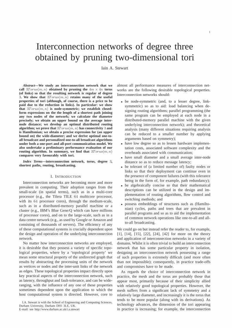
with addition modulo 4m or 4n, as appropriate. Theinterconnection network3Torus(4, 5) can be visualizedin Fig. 1 (as a pruned version ofTorus(16, 20) and withthe node(0, 0) in the centre of the diagram).
...
...
...
...
...
...
...
row 1
row 0
row 15
row 8
row 9
... ... ... ...
...
...
...
...
... ...... ...
...
...
...
col 0 col 1col 19 col 10col 11
......
... ...
Fig. 1. 3Torus(4, 5) (a pruned version ofTorus(16, 20)).
2
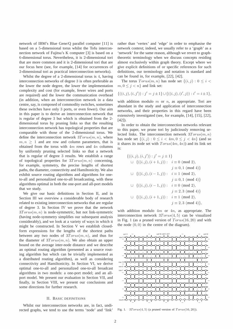
Note that there are alternative ways in which we mighthave defined3Torus(m,n). Consider all the cycles oflength 4 within 3Torus(m,n). If we condense each ofthese cycles into a single node, as is depicted in Fig. 2, thenwe obtain a network that can be described as a tessellationof the toroidal surface so that the faces are ‘diamonds’. Inmore detail, this ‘diamond’ network has node set{(i, j) :0 ≤ i < 2m, 0 ≤ j < 2n, i+ j ≡ 0 (mod 2)} and link set:
{((i, j), (i′, j′)) : (i′, j′) = (i, j) + (ǫ, δ),
with ǫ, δ ∈ {+1,−1}}
(with all addition componentwise and modulo2m or 2n,as appropriate). Consequently, we could have started withthis ‘diamond’ network and obtained3Torus(m,n) byamending the ‘diamond’ network so as to replace eachnode with a cycle of length4, similarly to when thecube-connected cycles network is obtained from ann-dimensional hypercube by replacing each node with a cycleof length n (see, for example, [42]). Note that viewing3Torus(m,n) in this way yields an alternative indexingfor the nodes, with a node determined by its coordinates(i, j) in the ‘diamond’ network and a ‘tag’ ofN , S, E orW (denoting ‘north’, ‘south’, ‘east’ or ‘west’).
...
...
...
...
...
...
...
... ... ... ...
...
...
...
...
...
...
...
...
... .........
... ...
Fig. 2. Condensing4-cycles in3Torus(4, 5) to get a ‘diamond’ network.
As a matter of fact, the ‘diamond’ network pictured inFig. 2 is actually one of the two (isomorphic) connectedcomponents of the Kronecker product of a cycle of length16 and a cycle of length10. TheKronecker productof thegraphG1 = (V1, E1) and the graphG2 = (V2, E2) wasfirst defined in [39] and has vertex setV1×V2 and edge set{((u1, u2), (v2, v2)) : (u1, v1) ∈ E1 and (u2, v2) ∈ E2}.In general (when constructing3Torus(m,n) as we did3Torus(4, 5) in Fig. 2), the starting ‘diamond’ networkis one of the two connected components of the Kroneckerproduct ofC4m andC2n. Such a ‘diamond’ network canalso be realised as atwo-dimensional circulantor an L-network(see [10] for definitions and further details).
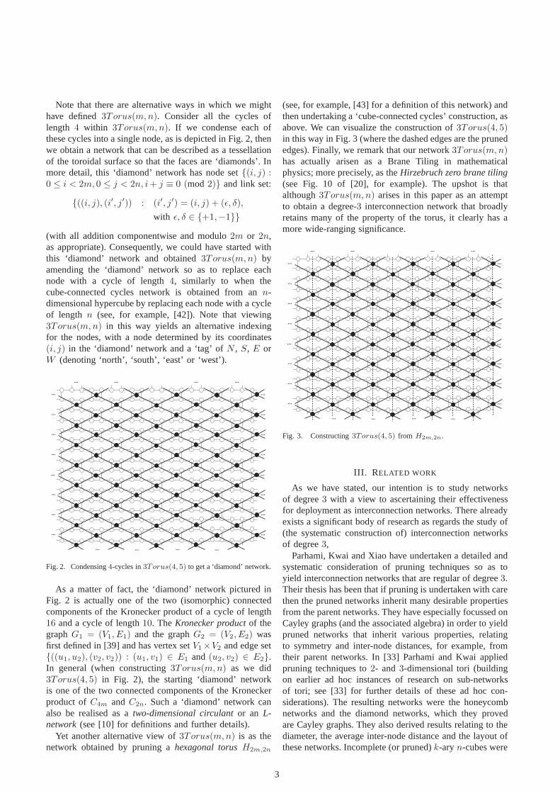
Yet another alternative view of3Torus(m,n) is as thenetwork obtained by pruning ahexagonal torusH2m,2n
(see, for example, [43] for a definition of this network) andthen undertaking a ‘cube-connected cycles’ construction,asabove. We can visualize the construction of3Torus(4, 5)in this way in Fig. 3 (where the dashed edges are the prunededges). Finally, we remark that our network3Torus(m,n)has actually arisen as a Brane Tiling in mathematicalphysics; more precisely, as theHirzebruch zero brane tiling(see Fig. 10 of [20], for example). The upshot is thatalthough3Torus(m,n) arises in this paper as an attemptto obtain a degree-3 interconnection network that broadlyretains many of the property of the torus, it clearly has amore wide-ranging significance.
...
...
...
...
...
...
...
... ... ... ...
...
...
...
...
...
...
...
...
... .........
... ...
Fig. 3. Constructing3Torus(4, 5) from H2m,2n.
III. R ELATED WORK
As we have stated, our intention is to study networksof degree3 with a view to ascertaining their effectivenessfor deployment as interconnection networks. There alreadyexists a significant body of research as regards the study of(the systematic construction of) interconnection networksof degree3,
Parhami, Kwai and Xiao have undertaken a detailed andsystematic consideration of pruning techniques so as toyield interconnection networks that are regular of degree3.Their thesis has been that if pruning is undertaken with carethen the pruned networks inherit many desirable propertiesfrom the parent networks. They have especially focussed onCayley graphs (and the associated algebra) in order to yieldpruned networks that inherit various properties, relatingto symmetry and inter-node distances, for example, fromtheir parent networks. In [33] Parhami and Kwai appliedpruning techniques to2- and 3-dimensional tori (buildingon earlier ad hoc instances of research on sub-networksof tori; see [33] for further details of these ad hoc con-siderations). The resulting networks were the honeycombnetworks and the diamond networks, which they provedare Cayley graphs. They also derived results relating to thediameter, the average inter-node distance and the layout ofthese networks. Incomplete (or pruned)k-aryn-cubes were
3
derived by Parhami and Kwai in [34] and properties relatingto symmetry, shortest paths, connectivity and Hamiltonicitywere established. Certain pruned3-dimensional tori werealso studied by Xiao and Parhami in [40], and in [41]Xiao and Parhami established general algebraic construc-tions (based on commutative groups) to develop pruningtechniques, which were used to improve known resultsrelating to honeycomb networks and to diamond networks.The algebraic approach of Parhami, Kwai and Xiao wassubsequently continued: in [35] where Rahman, Jiang,Masud and Horiguchi applied pruning techniques to thehierarchical torus network and studied properties relatingto shortest paths, average inter-node distance, bisectionwidth and VLSI layout area; and in [9] where an alge-braic construction related to group semidirect products wasdeveloped and used to provide a generalization of earlierpruning schemes. Beyond the concerted research effortdescribed above, there have also been various more isolatedconsiderations of interconnection networks of degree3,e.g., [6], [13], [25], [37], [44].
Regular graphs of degree3 (that is, cubic graphs) havealso been studied mathematically and in combinatorialchemistry with respect to some of the properties that happento be of interest in interconnection network design (notethat these graphs were not studied as potential interconnec-tion networksper se). These studies include, for example,[16], [17], [26], [29]–[31]. Also, theFoster Census[8],[12] was an enumeration of symmetric connected cubicedge-transitive graphs of order up to768. Interestingly,in [27] Hamiltonian cubic graphs from the Foster censuswere used as interconnection networks for computationalclusters undertaking efficient parallel molecular dynamicssimulations.
Finally, there is an extensive literature on other low-degree interconnection networks but where the degree is(at least)4. Noteworthy amongst this literature is the workin [10] and the references therein relating to manipulationsof tori but where the tori are not pruned and consequentlyalways have degree4. The interconnection networks studiedin [10] include tori, twisted and doubly twisted tori, toroidaldiagonal meshes, chordal rings, and circulant graphs. Otherrecent considerations of low-degree interconnection net-works can be found in [4], [18], where hexagonal mesh net-works, Gaussian networks and Eisenstein-Jacobi networksare studied (and the degree of the networks considered tendto be4 or 6), and in [36] where Spidergon-Donuts of degree5 are studied.
IV. SYMMETRY
We begin by proving that the network3Torus(m,n) isnode-symmetric. Recall that a networkG = (V,E) is node-symmetricif given any two nodesu andv, there exists anautomorphismmappingu to v; that is, a bijectionf : V →V such that if (u, v) ∈ E then (f(u), f(v)) ∈ E. Wedo this by constructing a set of basic automorphisms of3Torus(m,n) that can be composed to yield a requiredautomorphism.
Consider the following (node-) maps of3Torus(m,n):α : (i, j) 7→ (i, j + 4); β : (i, j) 7→ (i + 2, j);γ : (i, j) 7→ (i + 1, j + 2); ϕ : (i, j) 7→ (i′, j), wherei + i′ ≡ 1 (mod 4m); and ψ : (i, j) 7→ (i, j′′), wherej + j′′ ≡ 1 (mod 4n) (all values and their additions aremodulo 4m or modulo 4n as appropriate). All of thesemaps are clearly automorphisms:α, β andγ can be thoughtof as ‘translations’ horizontally, vertically and diagonally,respectively; andϕ andψ as ‘reflections’ in a horizontalline between row0 and row1 and in a vertical line betweencolumn0 and column1, respectively. By composing theseautomorphisms we can clearly map any node to any othernode. For example, in order to map(0, 0) to (3, 5) in3Torus(4, 5), we apply the automorphisms:ϕ (to take(0, 0) to (1, 0)); ψ (to take (1, 0) to (1, 1)); and γ2 (totake (1, 1) to (3, 5)).
However,3Torus(m,n) is not link-symmetric. Recallthat a network islink-symmetricif there exists an automor-phism mapping any given link to any other given link. Tosee this, the link((0, 0), (1, 0)) of 3Torus(m,n) lies in acycle of length4 whereas the link((1, 1), (1, 2)) does not.
Thus, we have proven the following.Theorem 1:The interconnection network3Torus(m,n)
is node-symmetric but not link-symmetric.We remark here that the network3Torus(m,n) does
possess a stronger property than node-symmetry in thatit is, in fact, aCayley graph(and consequently its node-symmetry follows immediately). However, a proof of thisfact involves combinatorial group theory and will be pre-sented elsewhere.
V. PATHS, ROUTING AND CONNECTIVITY
In this section, we look at some other aspects of3Torus(m,n) in relation to its adoption as an intercon-nection network: the lengths of shortest paths betweennodes; the average inter-node distance; its diameter; rout-ing algorithms; its connectivity; its wide-diameter; and itsHamiltonicity.
A. Shortest paths, the diameter and average distances
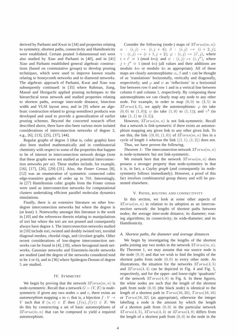
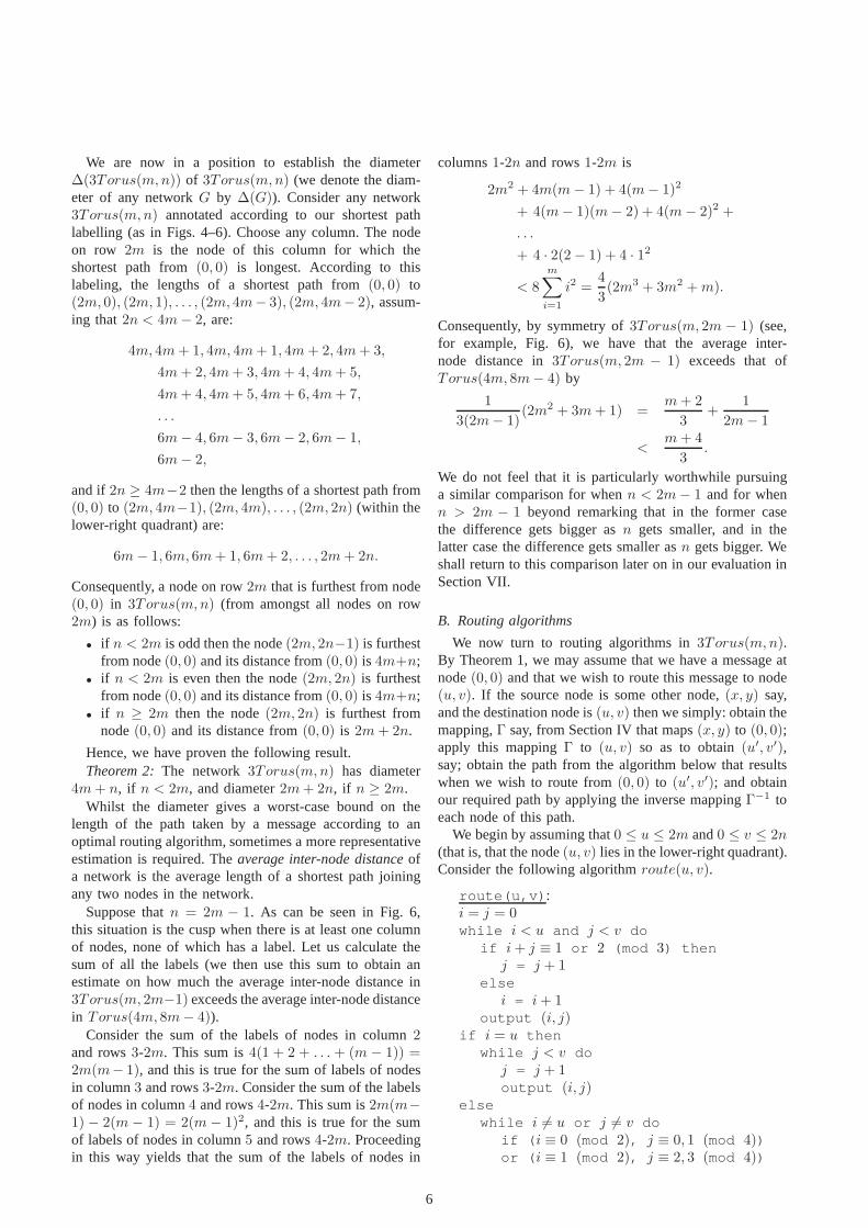
We begin by investigating the lengths of the shortestpaths joining any two nodes in the network3Torus(m,n).By Theorem 1, we may assume that our source node isthe node(0, 0) and that we wish to find the lengths of theshortest paths from node(0, 0) to every other node. Asillustrations, the situation for the networks3Torus(4, 5)and 3Torus(4, 4) can be depicted in Fig. 4 and Fig. 5,respectively, and for the upper- and lower-right ‘quadrants’of the network3Torus(4, 8) in Fig. 6. In these figures,the white nodes are such that the length of the shortestpath from node(0, 0) (the black node) is identical to thelength of a shortest path inTorus(16, 20), Torus(16, 16)or Torus(16, 32) (as appropriate), otherwise the integerlabelling a node is the amount by which the lengthof a shortest path from(0, 0) in the particular network3Torus(4, 5), 3Torus(4, 4) or 3Torus(4, 8) differs fromthe length of a shortest path from(0, 0) to the node in the
4
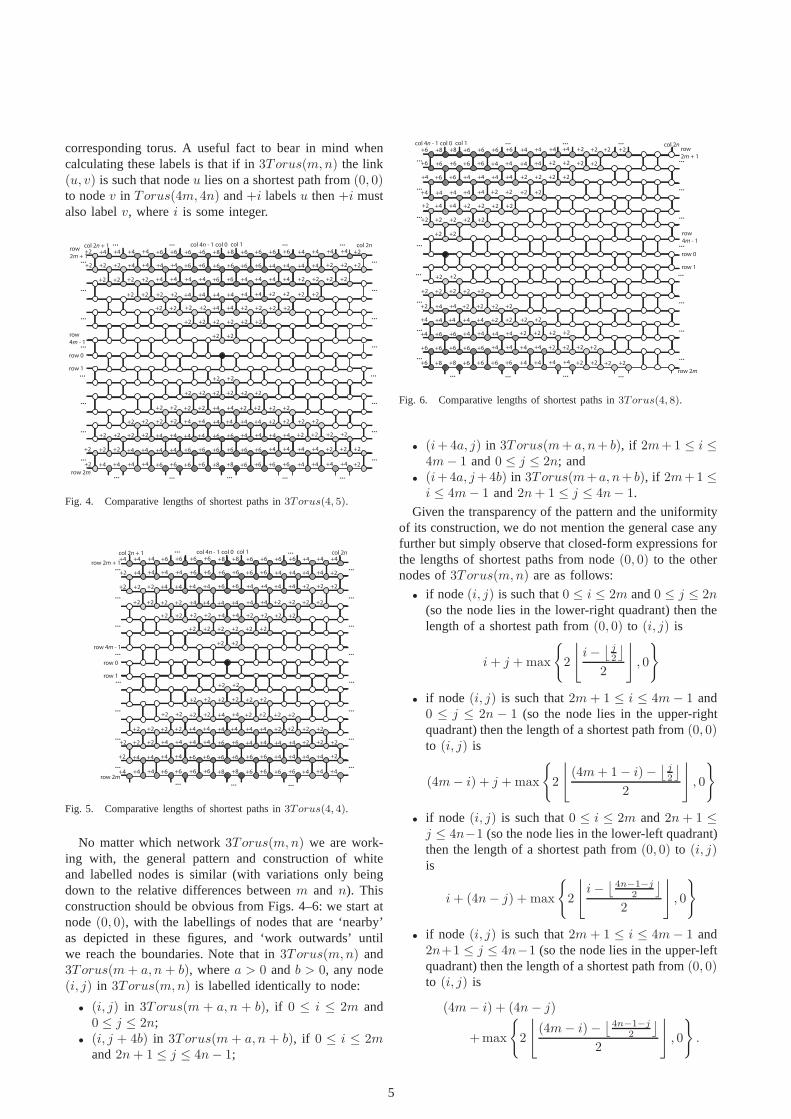
corresponding torus. A useful fact to bear in mind whencalculating these labels is that if in3Torus(m,n) the link(u, v) is such that nodeu lies on a shortest path from(0, 0)to nodev in Torus(4m, 4n) and+i labelsu then+i mustalso labelv, wherei is some integer.
...
...
...
...
...
...
...
row 1
row 0
row
4m - 1
row 2m
row
2m + 1
... ... ... ...
...
...
...
...
... ...... ...
...
...
...
col 0 col 1col 4n - 1 col 2ncol 2n + 1
+2 +2
+2 +2
+2 +2
+2 +2
+2 +2
+2 +2
+2 +2
+2 +2
+2 +2
+2 +2
+2 +2
+2 +2
+4 +4
+4 +4
+4 +4
+4
+4
+4 +4
+4 +4
+4
+4
+4 +4
+6 +6
+4 +4
+4 +4
+4 +4
+4 +4
+4 +4
+4 +4
+6 +6
+6 +6 +6 +6 +6 +6
+6 +6+6 +6 +8 +8 +6 +6
+2 +2
+2 +2
+2
+2
+4 +4
+2 +2
+4+4
+2 +2
+2 +2 +2
+2
+2 +2
+6 +6+4 +4 +4 +4+6 +6+6 +6 +8 +8 +6 +6+2 +4 +4 +4+4 +2
+2 +2 +2
+2 +2 +2 +2
+2 +2 +2 +2
+2 +2 +2 +2
+2 +2 +2 +2
+2 +2
+4 +4 +4 +4
+4 +4 +4 +4
+4 +4 +4 +4
+4 +4
+4 +4
+4 +4 +4 +4
+4 +4
+6 +6
+6 +6+6 +6 +6 +6 +4 +4
+2 +2
+2 +2 +2 +2
+2 +2 +2 +2
+2 +2 +2 +2
+2 +2 +2
......
... ...
Fig. 4. Comparative lengths of shortest paths in3Torus(4, 5).
...
...
...
...
...
...
...
row 1
row 0
row 4m - 1
row 2m
row 2m + 1
...
... ...
col 0 col 1col 4n - 1 col 2ncol 2n + 1
+2 +2
+2 +2
+2 +2
+2 +2
+2 +2
+2
+2 +2
+2 +2
+4 +4
+2
+6 +6
+6 +6
+4 +4
+4+4 +4
+4 +4
+4
+2 +2
+8 +8
+6 +6
+6 +6
+2
+2
+4 +4
+4 +4
+6 +6 +4 +4 +4 +4
+4 +4+6 +6 +6 +6 +4
+4 +4
+4 +4
+4
+2
+6 +6
+2 +2
+8 +8+6 +6 +4 +4+6 +6 +6 +6 +4+4 +6 +6
+2 +4 +4
+4 +4 +4 +4
+4+2 +2
+2 +2 +2 +2
+2 +2 +2 +2
+2 +2
+6 +6 +6 +6
+6 +6 +4 +4
+4 +4 +4
+4 +4
+4 +4
+2 +2 +2
+2
+4 +4
+4 +4+6 +6 +4 +4
+2 +2
+2 +2 +2
+2
......
...
...
+2 +2
+2 +2
+4 +4
+4 +4
+4 +4
+2 +2
+2
+2
+4 +4...
...
...
...
...
...
...
...
+2
+2+2 +2
+2
+2 +2 +2 +2
+2
Fig. 5. Comparative lengths of shortest paths in3Torus(4, 4).
No matter which network3Torus(m,n) we are work-ing with, the general pattern and construction of whiteand labelled nodes is similar (with variations only beingdown to the relative differences betweenm and n). Thisconstruction should be obvious from Figs. 4–6: we start atnode(0, 0), with the labellings of nodes that are ‘nearby’as depicted in these figures, and ‘work outwards’ untilwe reach the boundaries. Note that in3Torus(m,n) and3Torus(m+ a, n+ b), wherea > 0 andb > 0, any node(i, j) in 3Torus(m,n) is labelled identically to node:
• (i, j) in 3Torus(m + a, n + b), if 0 ≤ i ≤ 2m and0 ≤ j ≤ 2n;
• (i, j + 4b) in 3Torus(m + a, n + b), if 0 ≤ i ≤ 2mand2n+ 1 ≤ j ≤ 4n− 1;
...
...
...
...
...
...
...
row 1
row 0
row
4m - 1
row 2m
row
2m + 1
... ...
...
...
...
...
... ... ...
...
...
...
col 0 col 1col 4n - 1 col 2n
+2 +2
+2 +2 +2
+2 +2
+2 +2
+2 +2
+2
+2 +2
+4 +4
+4
+4
+4
+4
+4
+4
+4 +4 +4 +4
+4 +4
+4 +4
+4 +4
+6 +6
+6 +6 +6 +6 +6
+6 +6+6 +8 +8 +6 +6
+2 +2
+4+4
+2 +2
+2 +2 +2
+2
+2 +2
+4 +4+6 +6+6 +8 +8 +6 +6 +4
+2
+2 +2 +2
+2 +2
+4
+4 +4 +4
+4 +4
+4 +4
+4 +4 +4 +4
+4 +4
+6 +6
+6 +6+6 +6 +6 +4 +4
+2 +2
+2 +2 +2 +2
+2 +2 +2 +2
+2 +2 +2
+2
......
... ...
+2
+2 +2 +2
...
+2
+2 +2
+2
+2
+2 +2 +2+4
Fig. 6. Comparative lengths of shortest paths in3Torus(4, 8).
• (i+4a, j) in 3Torus(m+ a, n+ b), if 2m+1 ≤ i ≤4m− 1 and0 ≤ j ≤ 2n; and
• (i+4a, j+4b) in 3Torus(m+a, n+ b), if 2m+1 ≤i ≤ 4m− 1 and2n+ 1 ≤ j ≤ 4n− 1.
Given the transparency of the pattern and the uniformityof its construction, we do not mention the general case anyfurther but simply observe that closed-form expressions forthe lengths of shortest paths from node(0, 0) to the othernodes of3Torus(m,n) are as follows:
• if node(i, j) is such that0 ≤ i ≤ 2m and0 ≤ j ≤ 2n(so the node lies in the lower-right quadrant) then thelength of a shortest path from(0, 0) to (i, j) is
i+ j +max
{
2
⌊
i−⌊
j
2
⌋
2
⌋
, 0
}
• if node (i, j) is such that2m+ 1 ≤ i ≤ 4m− 1 and0 ≤ j ≤ 2n − 1 (so the node lies in the upper-rightquadrant) then the length of a shortest path from(0, 0)to (i, j) is
(4m− i) + j +max
{
2
⌊
(4m+ 1− i)−⌊
j
2
⌋
2
⌋
, 0
}
• if node (i, j) is such that0 ≤ i ≤ 2m and2n+ 1 ≤j ≤ 4n−1 (so the node lies in the lower-left quadrant)then the length of a shortest path from(0, 0) to (i, j)is
i+ (4n− j) + max
{
2
⌊
i−⌊
4n−1−j
2
⌋
2
⌋
, 0
}
• if node (i, j) is such that2m+ 1 ≤ i ≤ 4m− 1 and2n+1 ≤ j ≤ 4n−1 (so the node lies in the upper-leftquadrant) then the length of a shortest path from(0, 0)to (i, j) is
(4m− i) + (4n− j)
+max
{
2
⌊
(4m− i)−⌊
4n−1−j
2
⌋
2
⌋
, 0
}
.
5
We are now in a position to establish the diameter∆(3Torus(m,n)) of 3Torus(m,n) (we denote the diam-eter of any networkG by ∆(G)). Consider any network3Torus(m,n) annotated according to our shortest pathlabelling (as in Figs. 4–6). Choose any column. The nodeon row 2m is the node of this column for which theshortest path from(0, 0) is longest. According to thislabeling, the lengths of a shortest path from(0, 0) to(2m, 0), (2m, 1), . . . , (2m, 4m− 3), (2m, 4m− 2), assum-ing that2n < 4m− 2, are:
4m, 4m+ 1, 4m, 4m+ 1, 4m+ 2, 4m+ 3,
4m+ 2, 4m+ 3, 4m+ 4, 4m+ 5,
4m+ 4, 4m+ 5, 4m+ 6, 4m+ 7,
. . .
6m− 4, 6m− 3, 6m− 2, 6m− 1,
6m− 2,
and if 2n ≥ 4m−2 then the lengths of a shortest path from(0, 0) to (2m, 4m−1), (2m, 4m), . . . , (2m, 2n) (within thelower-right quadrant) are:
6m− 1, 6m, 6m+ 1, 6m+ 2, . . . , 2m+ 2n.
Consequently, a node on row2m that is furthest from node(0, 0) in 3Torus(m,n) (from amongst all nodes on row2m) is as follows:
• if n < 2m is odd then the node(2m, 2n−1) is furthestfrom node(0, 0) and its distance from(0, 0) is 4m+n;
• if n < 2m is even then the node(2m, 2n) is furthestfrom node(0, 0) and its distance from(0, 0) is 4m+n;
• if n ≥ 2m then the node(2m, 2n) is furthest fromnode(0, 0) and its distance from(0, 0) is 2m+ 2n.
Hence, we have proven the following result.Theorem 2:The network3Torus(m,n) has diameter
4m+ n, if n < 2m, and diameter2m+ 2n, if n ≥ 2m.Whilst the diameter gives a worst-case bound on the
length of the path taken by a message according to anoptimal routing algorithm, sometimes a more representativeestimation is required. Theaverage inter-node distanceofa network is the average length of a shortest path joiningany two nodes in the network.
Suppose thatn = 2m − 1. As can be seen in Fig. 6,this situation is the cusp when there is at least one columnof nodes, none of which has a label. Let us calculate thesum of all the labels (we then use this sum to obtain anestimate on how much the average inter-node distance in3Torus(m, 2m−1) exceeds the average inter-node distancein Torus(4m, 8m− 4)).
Consider the sum of the labels of nodes in column2and rows3-2m. This sum is4(1 + 2 + . . . + (m − 1)) =2m(m− 1), and this is true for the sum of labels of nodesin column3 and rows3-2m. Consider the sum of the labelsof nodes in column4 and rows4-2m. This sum is2m(m−1) − 2(m − 1) = 2(m − 1)2, and this is true for the sumof labels of nodes in column5 and rows4-2m. Proceedingin this way yields that the sum of the labels of nodes in
columns1-2n and rows1-2m is
2m2 + 4m(m− 1) + 4(m− 1)2
+ 4(m− 1)(m− 2) + 4(m− 2)2 +
. . .
+ 4 · 2(2− 1) + 4 · 12
< 8m∑
i=1
i2 =4
3(2m3 + 3m2 +m).
Consequently, by symmetry of3Torus(m, 2m − 1) (see,for example, Fig. 6), we have that the average inter-node distance in3Torus(m, 2m − 1) exceeds that ofTorus(4m, 8m− 4) by
1
3(2m− 1)(2m2 + 3m+ 1) =
m+ 2
3+
1
2m− 1
<m+ 4
3.
We do not feel that it is particularly worthwhile pursuinga similar comparison for whenn < 2m− 1 and for whenn > 2m − 1 beyond remarking that in the former casethe difference gets bigger asn gets smaller, and in thelatter case the difference gets smaller asn gets bigger. Weshall return to this comparison later on in our evaluation inSection VII.
B. Routing algorithms
We now turn to routing algorithms in3Torus(m,n).By Theorem 1, we may assume that we have a message atnode(0, 0) and that we wish to route this message to node(u, v). If the source node is some other node,(x, y) say,and the destination node is(u, v) then we simply: obtain themapping,Γ say, from Section IV that maps(x, y) to (0, 0);apply this mappingΓ to (u, v) so as to obtain(u′, v′),say; obtain the path from the algorithm below that resultswhen we wish to route from(0, 0) to (u′, v′); and obtainour required path by applying the inverse mappingΓ−1 toeach node of this path.
We begin by assuming that0 ≤ u ≤ 2m and0 ≤ v ≤ 2n(that is, that the node(u, v) lies in the lower-right quadrant).Consider the following algorithmroute(u, v).
route(u,v):i = j = 0while i < u and j < v do
if i+ j ≡ 1 or 2 (mod 3) thenj = j + 1
elsei = i+ 1
output (i, j)if i = u then
while j < v doj = j + 1output (i, j)
elsewhile i 6= u or j 6= v do
if (i ≡ 0 (mod 2), j ≡ 0, 1 (mod 4))or (i ≡ 1 (mod 2), j ≡ 2, 3 (mod 4))
6
theni = i+ 1
elseif j ≡ 1 (mod 2) then
j = j + 1else
j = j − 1output (i, j)
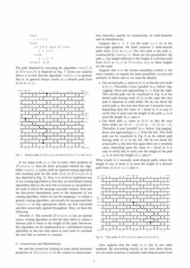
The path obtained by executing the algorithmroute(7, 5)in 3Torus(4, 8) is depicted in Fig. 7. Given our analysisabove, it is clear that the algorithmroute(u, v) is optimal;that is, in general always results in a shortest path from(0, 0) to (u, v).
...
...
...
...
...
...
...
row 1
row 0
row
4m - 1
row 2m
row
2m + 1
... ...
...
...
...
...
... ... ...
...
...
...
col 0 col 1col 4n - 1 col 2n
......
... ...
...
Fig. 7. Shortest paths in3Torus(4, 8) from (0, 0) to (7, 5) and(9, 6).
If our target node(u, v) lies in some other quadrant of3Torus(m,n) then the basic principles behind the algo-rithm route(u, v) easily yield an optimal routing algorithm(the resulting path for the node(9, 6) in 3Torus(4, 8) isalso depicted in Fig. 7). Also, it is trivial to implement anyof our routing algorithms so that they are distributed routingalgorithms (that is, the next link to traverse is calculatedbythe node at which the message currently resides). Note thatthe discussion immediately prior to the statement of ourrouting algorithm, where we use the mappingΓ to obtain ageneric routing algorithm, can trivially be incorporated intoroute(u, v) so that appropriate offsets are first calculatedand then universally applied throughout. Thus, we have thefollowing.
Theorem 3:The network3Torus(m,n) has an optimalsource routing algorithm so that the time taken to output ashortest path is linear in the length of this path. Moreover,this algorithm can be implemented as a distributed routingalgorithm so that the time taken at each node to calculatethe next link to traverse is constant.
C. Connectivity and Hamiltonicity
We end this section by looking at some useful structuralproperties of3Torus(m,n) in the context of interconnec-
tion networks, namely its connectivity, its wide-diameterand its Hamiltonicity.
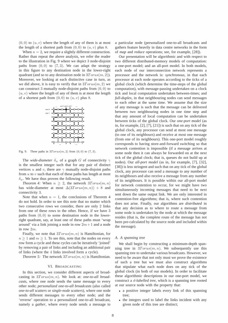
Suppose thatn ≥ 3. Let the node(u, v) lie in thelower-right quadrant. We shall construct3 node-disjointpaths from(0, 0) to (u, v). Our first path is the pathρ1constructed byroute(u, v). There are two possibilities: thepathρ1 has length different to the length of a shortest pathfrom (0, 0) to (u, v) in Torus(4m, 4n); or these lengthsare the same.
Suppose that it is the former possibility (which is themore complex; as regards the latter possibility, we proceedsimilarly to below and so we omit the details).
• Our second pathρ2 starts at(0, 0) so that the next nodeis (0, 1). Thereafter, it runs ‘parallel’ toρ1 before ‘zig-zagging’ down and approaching(u, v) from the right.This second path can be visualized in Fig. 8 as thedotted path leaving node(0, 0) to the right (the firstpath is depicted in solid bold). We do not detail theactual pathρ2 but note that there are4 essential cases,depending upon the value ofv (mod 4). It is easy toverify that in each case the length of the pathρ2 is atmost the length ofρ1 plus 8.
• Our third path ρ3 starts at(0, 0) so that the nextthree nodes are(0, 4n − 1), (0, 4n − 2), (0, 4n − 3).Thereafter, it runs ‘parallel’ toρ1 before ‘zig-zagging’down and approaching(u, v) from the left. This thirdpath can be visualized in Fig. 8 as the dotted pathleaving node(0, 0) to the left. We do not detail theactual pathρ3 but note that again there are4 essentialcases, depending upon the value ofv (mod 4). It iseasy to verify that in each case the length of the pathρ3 is at most the length ofρ1 plus 8.
What results is3 mutually node-disjoint paths where thelength of any of them is at most the length of a shortestpath from(0, 0) to (u, v) plus 8.
...
...
...
...
...
...
...
row 1
row 0
row
4m - 1
row 2m
row
2m + 1
... ... ... ...
...
...
...
...
... ...... ...
...
...
...
col 0 col 1col 4n - 1 col 2ncol 2n + 1
......
... ...
Fig. 8. Three paths in3Torus(4, 5) from (0, 0) to (6, 5).
Now suppose that the node(u, v) lies in any otherquadrant. By proceeding exactly as we have done above,we can easily construct3 mutually node-disjoint paths from
7
(0, 0) to (u, v) where the length of any of them is at mostthe length of a shortest path from(0, 0) to (u, v) plus 8.
Whenn = 2, we require a slightly different construction.Rather than repeat the above analysis, we refer the readerto the illustration in Fig. 9 where we depict3 node-disjointpaths from (0, 0) to (7, 3). We can adapt the strategyin this figure to any destination node in the lower-rightquadrant (and so to any destination node in3Torus(m, 2)).Moreover, we looking at each distinctive case in turn, aswe did above, it is easy to verify that in3Torus(m, 2) wecan construct3 mutually node-disjoint paths from(0, 0) to(u, v) where the length of any of them is at most the lengthof a shortest path from(0, 0) to (u, v) plus 8.
row 1
row 0
col 0 col 1col 7
... ...
... ...
Fig. 9. Three paths in3Torus(m, 2) from (0, 0) to (7, 3).
The wide-diameterδw of a graphG of connectivityγis the smallest integer such that for any pair of distinctverticesu andv, there areγ mutually node-disjoint pathsfrom u to v such that each of these paths has length at mostδw. We have thus proven the following result.
Theorem 4:When n ≥ 2, the network3Torus(m,n)has wide-diameter at most∆(3Torus(m,n)) + 8 andconnectivity3.
Note that whenn = 1, the conclusions of Theorem 4do not hold. In order to see this note that no matter whichtwo consecutive rows we consider, there are only2 linksfrom one of these rows to the other. Hence, if we have3paths from(0, 0) to some destination node in the lower-right quadrant, say, at least one of these paths must ‘wraparound’ via a link joining a node in row2m+1 and a nodein row 2m.
Finally, we note that3Torus(m,n) is Hamiltonian, forn ≥ 1 andm ≥ 1. To see this, note that the nodes on everyrow form a cycle and these cycles can be iteratively ‘joined’by removing a pair of links and including an additional pairof links (where the4 links involved form a cycle).
Theorem 5:The network3Torus(m,n) is Hamiltonian.
VI. B ROADCASTING
In this section, we consider different aspects of broad-casting in 3Torus(m,n). We look at: one-to-all broad-casts, where one node sends the same message to everyother node;personalized one-to-all broadcasts(also calledone-to-all scattersor single-node scatters), where one nodesends different messages to every other node; and the‘reverse’ operation to a personalized one-to-all broadcast,namely agather, where every node sends a message to
a particular node (personalized one-to-all broadcasts andgathers feature heavily in data centre networks in the formof mapand reduceoperations; see, for example, [28]).
Our presentation will be algorithmic and with respect totwo different distributed-memory models of computation:a one-port model; and an all-port model. In both models,each node of our interconnection network represents aprocessor and the network is:synchronous, in that eachprocessor at each node operates according to the ticks of aglobal clock (which determine the time-steps of the globalcomputation), with message-passing undertaken on a clocktick and local computation undertaken between-times; andfull-duplex, in that neighbouring nodes can send messagesto each other at the same time. We assume that the sizeof any message is such that the message can be deliveredbetween two neighbouring nodes in one time step andthat any amount of local computation can be undertakenbetween ticks of the global clock. Ourone-port model(asin, for example, [2], [7], [21]) is such that on any tick of theglobal clock, any processor can send at most one message(to one of its neighbours) and receive at most one message(from one of its neighbours). This one-port model roughlycorresponds to having store-and-forward switching so thatnetwork contention is impossible (if a message arrives atsome node then it can always be forwarded on at the nexttick of the global clock; that is, queues do not build up atnodes). Ourall-port model (as in, for example, [7], [32],[38]) is less stringent and such that on any tick of the globalclock, any processor can send a message to any number ofits neighbours and also receive a message from any numberof its neighbours. It is possible within our all-port modelfor network contention to occur, for we might have twosimultaneously incoming messages that need to be nextsent down the same output link. We are only interested incontention-free algorithms; that is, where such contentiondoes not arise. Finally, our algorithms aredistributed inthat any decision as to where to route a message fromsome node is undertaken by the node at which the messageresides (that is, the complete route of the message has notbeen pre-calculated by the source node and included withinthe message).
A. A spanning tree
We shall begin by constructing a minimum-depth span-ning tree in 3Torus(m,n). We subsequently use thisspanning tree to undertake various broadcasts. However, weneed to be aware that not only must we prove the existenceof such a tree but we must also construct algorithmsthat stipulate what each node does on any tick of theglobal clock (in both of our models). In order to facilitatethese algorithmic descriptions in our one-port model, weconstruct ad-labelled tree, which is a spanning tree rootedat our source node with the property that:
• a positive integer labels every link of this spanningtree;
• the integers used to label the links incident with anygiven node of this tree are distinct;
8
• the integer used to label the link joining some (non-root) node to its parent in this tree is less than any ofthe integers used to label any link from this node toone of its children; and
• the integers used as labels come from the set{1, 2,. . . , d}, for somed, with every integer from this setappearing as a label at least once.
Given somed-labelled tree, we perform a one-to-all broad-cast in our one-port model, for example, as follows. Themessageǫ starts at the root node and on theith tick of theglobal clock, wherei ∈ {1, 2, . . . , d}, any nodeu joined toa childv via a link labelledi sends the messageǫ, currentlyat u, to v. A simple induction yields that if we have ad-labelled spanning tree then the resulting algorithm is well-defined; that is, is such that when a nodeu wishes to sendthe messageǫ, this message does indeed reside atu.
Theorem 6:Define d = ∆(3Torus(m,n)) and let ube any node of3Torus(m,n). There exists ad-labelledspanning treeTu of depthd that is rooted atu so that forevery nodev of 3Torus(m,n), the length of the path fromu to v in Tu is equal to the length of a shortest path fromu to v in 3Torus(m,n).
Proof: By Theorem 1, we may assume thatu = (0, 0).There are two case: when2m ≤ n; and when2m > n.
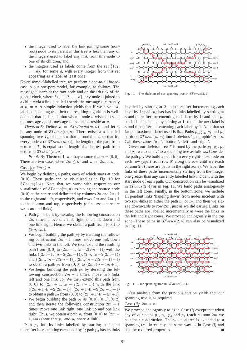
Case (i): 2m ≤ n.
We begin by defining4 paths, each of which starts at node(0, 0). These paths can be visualized as in Fig. 10 for3Torus(2, 4). Note that we work with respect to ourvisualization of3Torus(m,n) as having the source node(0, 0) at the centre and delimitted by columns2n and2n+1to the right and left, respectively, and rows2m and2m+1to the bottom and top, respectively (of course, there arewrap-around links).
• Pathp1 is built by iterating the following construction2m times: move one link right, one link down andone link right. Hence, we obtain a path from(0, 0) to(2m, 4m).
• We begin building the pathp2 by iterating the follow-ing construction2m − 1 times: move one link downand two links to the left. We then extend the resultingpath from(0, 0) to (2m−1, 4n−2(2m−1)) with thelinks ((2m−1, 4n−2(2m−1)), (2m, 4n−2(2m−1))and((2m, 4n−2(2m−1)), (2m, 4n−2(2m−1)−1)to obtain a pathp2 from (0, 0) to (2m, 4n− 4m+1).
• We begin building the pathp3 by iterating the fol-lowing construction2m − 1 times: move two linksleft and one link up. We then extend this path from(0, 0) to (2m + 1, 4n − 2(2m − 1)) with the link((2m+1, 4n−2(2m−1)), (2m+1, 4n−2(2m−1)−1)to obtain a pathp2 from (0, 0) to (2m+1, 4n−4m+1).
• We begin building the pathp4 as (0, 0), (0, 1), (0, 2)and then iterate the following construction2m − 1times: move one link right, one link up and one linkright. Thus, we obtain a pathp4 from (0, 0) to (2m+1, 4m) (note thatp1 andp4 share a link).
Path p1 has its links labelled by starting at1 andthereafter incrementing each label by1; pathp2 has its links
434
4 35
7 6
910
8
11
12
10
...
col 0 col 1...
7
3
2
1
4
6
5
2
row 1
row 0
row 7
...
...
col 15
row 1
row 0
row 7
...
...
col 0 col 1... col 15
3
...
9 10
8
11
12
5
76
9
8
11 12
57 6
9108
1112
path p1path p
2
path p4
path p3
Fig. 10. The skeleton of our spanning tree in3Torus(2, 4).
labelled by starting at2 and thereafter incrementing eachlabel by1; pathp3 has has its links labelled by starting at3 and thereafter incrementing each label by1; and pathp4has its links labelled by starting at1 so that the next label is3 and thereafter incrementing each label by1. Note that sofar the maximum label used is6m. Pathsp1, p2, p3 andp4partition3Torus(m,n) into 4 obvious ‘geographic’ zones.Call these zones ‘top’, ‘bottom’, ‘left’ and ‘right’.
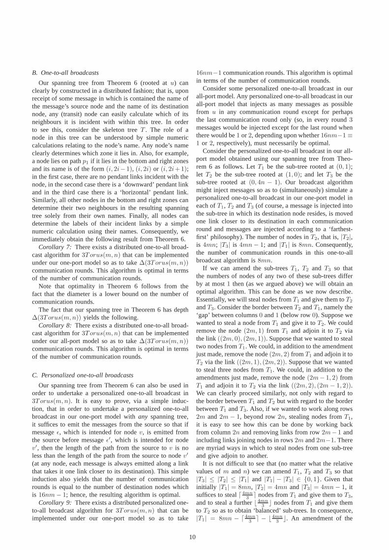
Given our skeleton treeT formed by the pathsp1, p2, p3andp4, we extendT to a spanning tree as follows. Considerthe pathp1. We build a path from every right-most node oneach row (apart from row0) along the row until we reachcolumn2n (these are paths in the right zone). We label thelinks of these paths incrementally starting from the integerone greater than any currently labelled link incident with thestart node of each path. Our construction can be visualizedin 3Torus(2, 4) as in Fig. 11. We build paths analogouslyin the left zone. Finally, in the bottom zone, we includeall pendant links ‘hanging down’ from nodes incident withtwo row-links in either the pathp1 or p2, and then we zig-zag downwards to row2m, just as we did earlier. Links onthese paths are labelled incrementally as were the links inthe left and right zones. We proceed analogously in the topzone. These paths in3Torus(2, 4) can also be visualizedin Fig. 11.
4 35
7 6
910
8
11
12
10
...
col 0 col 1...
7
3
2
1
4
6
4
5
23
row 1
row 0
row 7
...
...
col 15
row 1
row 0
row 7
...
...
col 0 col 1... col 15
3
...
9 10
8
11
12
576
98
11
12
4
57 6
9108
11
12
9 10
8 9
8 9
9 10
12
11
10
10
1112
66 7
7
5 5
1111
8 8
6
77
6
9 8 8 9
109910
11 10 10 11 1212
9
8
8
9
77 6
6
8 8
9 91111 1010
11 10 10 11 1212
5 5
677
6
8 899
10
9
9
10
12
11
10
10
11
12
Fig. 11. Our spanning tree in3Torus(2, 4).
Our analysis from the previous section yields that ourspanning tree is as required.
Case (ii ): 2m > n.
We proceed analogously to as in Case (i) except that whenany of our pathsp1, p2, p3 and p4 reach column2m wehalt their construction. The skeleton tree is extended to aspanning tree in exactly the same way as in Case (i) andhas the required properties.
9
B. One-to-all broadcasts
Our spanning tree from Theorem 6 (rooted atu) canclearly by constructed in a distributed fashion; that is, uponreceipt of some message in which is contained the name ofthe message’s source node and the name of its destinationnode, any (transit) node can easily calculate which of itsneighbours it is incident with within this tree. In orderto see this, consider the skeleton treeT . The role of anode in this tree can be understood by simple numericcalculations relating to the node’s name. Any node’s nameclearly determines which zone it lies in. Also, for example,a node lies on pathp1 if it lies in the bottom and right zonesand its name is of the form(i, 2i− 1), (i, 2i) or (i, 2i+1);in the first case, there are no pendant links incident with thenode, in the second case there is a ‘downward’ pendant linkand in the third case there is a ‘horizontal’ pendant link.Similarly, all other nodes in the bottom and right zones candetermine their two neighbours in the resulting spanningtree solely from their own names. Finally, all nodes candetermine the labels of their incident links by a simplenumeric calculation using their names. Consequently, weimmediately obtain the following result from Theorem 6.
Corollary 7: There exists a distributed one-to-all broad-cast algorithm for3Torus(m,n) that can be implementedunder our one-port model so as to take∆(3Torus(m,n))communication rounds. This algorithm is optimal in termsof the number of communication rounds.
Note that optimality in Theorem 6 follows from thefact that the diameter is a lower bound on the number ofcommunication rounds.
The fact that our spanning tree in Theorem 6 has depth∆(3Torus(m,n)) yields the following.
Corollary 8: There exists a distributed one-to-all broad-cast algorithm for3Torus(m,n) that can be implementedunder our all-port model so as to take∆(3Torus(m,n))communication rounds. This algorithm is optimal in termsof the number of communication rounds.
C. Personalized one-to-all broadcasts
Our spanning tree from Theorem 6 can also be used inorder to undertake a personalized one-to-all broadcast in3Torus(m,n). It is easy to prove, via a simple induc-tion, that in order to undertake a personalized one-to-allbroadcast in our one-port model withany spanning tree,it suffices to emit the messages from the source so that ifmessageǫ, which is intended for nodev, is emitted fromthe source before messageǫ′, which is intended for nodev′, then the length of the path from the source tov is noless than the length of the path from the source to nodev′
(at any node, each message is always emitted along a linkthat takes it one link closer to its destination). This simpleinduction also yields that the number of communicationrounds is equal to the number of destination nodes whichis 16nm− 1; hence, the resulting algorithm is optimal.
Corollary 9: There exists a distributed personalized one-to-all broadcast algorithm for3Torus(m,n) that can beimplemented under our one-port model so as to take
16nm−1 communication rounds. This algorithm is optimalin terms of the number of communication rounds.
Consider some personalized one-to-all broadcast in ourall-port model. Any personalized one-to-all broadcast in ourall-port model that injects as many messages as possiblefrom u in any communication round except for perhapsthe last communication round only (so, in every round3messages would be injected except for the last round whenthere would be1 or 2, depending upon whether16nm−1 ≡1 or 2, respectively), must necessarily be optimal.
Consider the personalized one-to-all broadcast in our all-port model obtained using our spanning tree from Theo-rem 6 as follows. LetT1 be the sub-tree rooted at(0, 1);let T2 be the sub-tree rooted at(1, 0); and letT3 be thesub-tree rooted at(0, 4n − 1). Our broadcast algorithmmight inject messages so as to (simultaneously) simulate apersonalized one-to-all broadcast in our one-port model ineach ofT1, T2 andT3 (of course, a message is injected intothe sub-tree in which its destination node resides, is movedone link closer to its destination in each communicationround and messages are injected according to a ‘farthest-first’ philosophy). The number of nodes inT2, that is,|T2|,is 4mn; |T3| is 4mn− 1; and |T1| is 8mn. Consequently,the number of communication rounds in this one-to-allbroadcast algorithm is8mn.
If we can amend the sub-treesT1, T2 and T3 so thatthe numbers of nodes of any two of these sub-trees differby at most1 then (as we argued above) we will obtain anoptimal algorithm. This can be done as we now describe.Essentially, we will steal nodes fromT1 and give them toT2andT3. Consider the border betweenT2 andT1, namely the‘gap’ between columns0 and1 (below row0). Suppose wewanted to steal a node fromT1 and give it toT2. We couldremove the node(2m, 1) from T1 and adjoin it toT2 viathe link ((2m, 0), (2m, 1)). Suppose that we wanted to stealtwo nodes fromT1. We could, in addition to the amendmentjust made, remove the node(2m, 2) from T1 and adjoin it toT2 via the link ((2m, 1), (2m, 2)). Suppose that we wantedto steal three nodes fromT1. We could, in addition to theamendments just made, remove the node(2m− 1, 2) fromT1 and adjoin it toT2 via the link ((2m, 2), (2m− 1, 2)).We can clearly proceed similarly, not only with regard tothe border betweenT1 andT2 but with regard to the borderbetweenT1 andT3. Also, if we wanted to work along rows2m and2m− 1, beyond row2n, stealing nodes fromT1,it is easy to see how this can be done by working backfrom column2n and removing links from row2m− 1 andincluding links joining nodes in rows2m and2m−1. Thereare myriad ways in which to steal nodes from one sub-treeand give adjoin to another.
It is not difficult to see that (no matter what the relativevalues ofm andn) we can amendT1, T2 andT3 so that|T3| ≤ |T2| ≤ |T1| and |T1| − |T3| ∈ {0, 1}. Given thatinitially |T1| = 8mn, |T2| = 4mn and |T3| = 4mn− 1, itsuffices to steal⌈ 4mn
3⌉ nodes fromT1 and give them toT3,
and to steal a further⌊ 4mn3
⌋ nodes fromT1 and give themto T2 so as to obtain ‘balanced’ sub-trees. In consequence,|T1| = 8mn − ⌈ 4mn
3⌉ − ⌊ 4mn
3⌋. An amendment of the
10
sub-treesT1, T2 and T3 (in the above fashion) in thecase of 3Torus(2, 4) can be visualized as in Fig. 12,where the roots of the sub-trees are grey nodes, wherethe dashed lines are the new borders between the amendedsub-trees and where|T1| = 43 and |T2| = |T3| = 42.Moreover, with more precision, we could clearly developan algorithm that every node of3Torus(m,n) (that is,processor) could apply locally in order to give its amendedlinks in the resulting spanning tree (such an algorithmwould be a straightforward, if messy, numeric calculationwith parametersm, n and the row and column of thenode). Hence, by our discussion above (and including thatimmediately following Corollary 9), we have the followingresult.
...
col 0 col 1...
row 1
row 0
row 7
...
...
col 15
row 1
row 0
row 7
...
...
col 0 col 1... col 15
...
Fig. 12. Our amended sub-trees in3Torus(2, 4).
Corollary 10: There exists a distributed personalizedone-to-all broadcast algorithm for3Torus(m,n) that canbe implemented under our all-port model so as to take8mn−⌈ 4mn
3⌉− ⌊ 4mn
3⌋ communication rounds. This algo-
rithm is optimal in terms of the number of communicationrounds.
D. Gathers
Finally, consider a gather in3Torus(m,n). In our one-port model, we can clearly use our spanning-tree fromTheorem 6 in order to undertake a gather that is optimal(essentially, we just ‘reverse’ the personalized one-to-allbroadcast from Corollary 9; the resulting algorithm stillconforms to our one-port model). As regards our person-alized one-to-all broadcast in our all-port model, againby ‘reversing’ it we obtain a gather, with this algorithmbeing optimal for the reason detailed immediately afterCorollary 9 (this is immediate given that the algorithmimplicit in Corollary 10 consists of3 independent ‘one-portalgorithms’). Hence, we have the following results.
Corollary 11: There exists a distributed gather algorithmfor 3Torus(m,n) that can be implemented under ourone-port model so as to take16mn − 1 communicationrounds. This algorithm is optimal in terms of the numberof communication rounds.
Corollary 12: There exists a distributed gather algorithmfor 3Torus(m,n) that can be implemented under our all-port model so as to take8mn− ⌈ 4mn
3⌉ − ⌊ 4mn
3⌋ commu-
nication rounds. This algorithm is optimal in terms of thenumber of communication rounds.
VII. E VALUATION
Having derived some properties of3Torus(m,n), wenow compare3Torus(m,n) with Torus(4m, 4n), whichhas the same number of nodes (note that the primarymotivation of the design of3Torus(m,n) is as a ‘degree-3’ version of a torus). As we shall see, the comparison isgenerally favourable although (as might be expected) thereis a price to be paid by pruning and consequent degreereduction. Our evaluation comes in two parts: first, we com-pare3Torus(m,n) andTorus(4m, 4n) in terms of theirstructural (graph-theoretic) properties (that are pertinentin their usage as interconnection networks); and second,we undertake a preliminary performance evaluation ofrouting algorithms in3Torus(m,n) andTorus(4m, 4n).Our performance evaluation is but a prelude to a morethorough simulation (as we explain in our conclusions inSection VIII).
A. A structural comparison
First, we note from Theorem 1 that3Torus(m,n) isnode-symmetric but not link-symmetric. It is well-known(and easy to see) thatTorus(N,N) is both node- andlink-symmetric; however, note thatTorus(N1, N2) is nolonger link-symmetric ifN1 6= N2. Link-symmetry can beimportant in terms of load balancing. However, the lack oflink-symmetry might be ameliorated depending upon theapplication, for there is still a degree of link-symmetry in3Torus(m,n) in that: there is clearly an automorphismmapping any column-link to any other column-link; andthe row-links partition into two disjoint sets,E4 andE8, sothat there is an automorphism mapping any row-link ofE4
(resp.E8) to any other row-link ofE4 (resp.E8) (in group-theoretic terms, there are only three orbits of edges underthe action of the automorphism group of3Torus(m,n);the setsE4 andE8 are so named so as to reflect the lengthof a shortest cycle in which the row-link lies).
As regards diameters, when we compare3Torus(m,n)with Torus(4m, 4n) we can immediately see fromTheorem 2 that ∆(3Torus(m,n)) is identical to∆(Torus(4m, 4n)) = 2m + 2n, if n ≥ 2m, andgreater than∆(Torus(4m, 4n)) by 2m − n, if n <
2m. For the special case wherem = n we have that∆(Torus(4m, 4m)) = 4m and∆(3Torus(m,m)) = 5m.Consequently, depending onm andn, we might be able tobuild 3Torus(m,n) so that we lose nothing in comparisonwith the diameter ofTorus(4m, 4n). Our optimal andeasy-to-implement routing algorithm ensures that we canefficiently utilize this state of affairs.
As regards the average inter-node distance, that ofTorus(4m, 4n) is better than that of3Torus(m,n) (aswe might expect). The quality of the average inter-nodedistance of 3Torus(m,n) in comparison with that ofTorus(4m, 4n) depends upon the relative values ofm andn with the largern is in comparison tom, the better. Justas when we compared the diameters ofTorus(4m, 4n) and3Torus(m,n), it makes sense to try and increasen withrespect tom.
11
From [23], the wide-diameter ofTorus(4m, 4n) is∆(Torus(4m, 4n))+1, if bothm andn are greater than1,and∆(Torus(4m, 4n)) + 2, if eitherm or n is equal to1and the other component is at least3. From Theorem 4, thewide-diameter of3Torus(m,n) is ∆(3Torus(m,n)) + 8which is still relatively good in comparison (in that it isdifferent from the diameter by a small constant value). Ofcourse, the lower degree of3Torus(m,n) in comparisonwith Torus(4m, 4n) means that we have less connectivity(and so less path diversity and capacity to tolerant faults);nevertheless, the connectivity of3Torus(m,n) is equal toits degree (which is all that we can hope for). As regardsHamiltonicity, by Theorem 53Torus(m,n) is Hamilto-nian, just likeTorus(4m, 4n). However, there cannot existedge-disjoint Hamiltonian cycles in3Torus(m,n) (as thedegree is3) whereas it is well-known thatTorus(4m, 4n)does have edge-disjoint Hamiltonian cycles (see, for exam-ple, [5]).
In [2], optimal one-to-all and personalized one-to-allbroadcast algorithms for tori were given for the one-port model of computation; in [7], [19] optimal one-to-allbroadcast algorithms for tori were given for the all-portmodel of computation; and in [19] optimal personalizedone-to-all broadcast algorithms for tori were given for theall-port model of computation. Given our comments aboveas regards the relative diameters of3Torus(m,n) andTorus(4m, 4n), along with Corollaries 7, 8, 9 and 10,3Torus(m,n) behaves comparably toTorus(4m, 4n) interms of one-to-all broadcasts.
B. Simulating routing algorithms
Our performance evaluation compares our routing al-gorithm for 3Torus(m,n) with the XY-routing algorithmfor Torus(4m, 4n). Recall, theXY-routing algorithmina torus is simply to route along a row until the messagereaches a node in the same column as the destination, andthen to route along the column, with both the X-route andthe Y-route being the shortest from the two possibilities.Given that we have a precise closed form of the length ofany route obtained within3Torus(m,n) (via our routingalgorithm), we focus on loads arising (or, more precisely,on the distribution of generated paths over each link) in ourchosen traffic pattern.
As regards the preliminary nature of our performanceevaluation, the primary purpose of the research in thispaper is the introduction of the interconnection network3Torus(m,n), together with a structural analysis of itsviability as a replacement network for a torus in a ‘degree-3’ context; that is, a full and proper performance evaluationis beyond our scope and requires additional research asregards more sophisticated (adaptive) routing algorithmsand also all-to-all broadcasts (we have more to say in Sec-tion VIII). Nevertheless, we are in a position to undertakea preliminary experimental analysis. Of particular interestto us is how the relative sizes of the parametersm andn in 3Torus(m,n) impact upon routing performance (interms of loads arising and the balance of these loads),
and of how the routing performance in3Torus(m,n) andTorus(4m, 4n) (its natural counterpart) differ.
We assume therandom traffic patternwhere every nodeof a network (simultaneously) sends a message to someuniformly randomly chosen node (possibly itself). Ouranalysis consists of undertaking numerous trials of randomtraffic messaging (actually,1000 trials), with respect to ourrouting algorithms, so as to acquire data as regards thecumulative loads on (that is, number of generated pathsusing) each individual link in the network. We vary theparametersm andn in 3Torus(m,n) and compare the re-sulting loads with the loads obtained (using XY-routing) inTorus(4m, 4n). Given the structure of3Torus(m,n) andTorus(4m, 4n), we also consider row-links and column-links separately; indeed, for3Torus(m,n) we partitionrow-links into those that are contained within a cycle oflength 4, which we callrow4-links, and those that aren’t,which we callrow8-links (cf. our comments above on link-symmetry).
From our structural analysis, we have seen that thesituation whenn = 2m− 1 would appear to be a cusp atwhich the behaviour of3Torus(m,n) changes. One aim ofour experiments is to investigate around this threshold. Tothis end, for a fixedm ranging from2 to 12, we allown tovary at intervals of (the integer part of)m
2from m
2through
m and 2m up to 7m2
(which we deem sufficiently large).For each scenario, we collect the load on each link (asdescribed above and with data from1000 trials) so that wemight calculate the average link load and also the standarddeviation of the link load, so that we might obtain someappreciation of the balance of loads across all links.
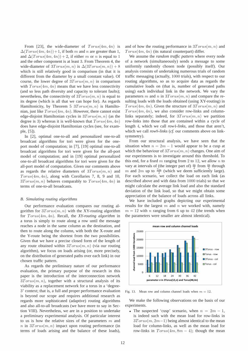
We have included graphs depicting our experimentalresults for the largestm and n we worked with, namelym = 12 with n ranging from6 up to 42 (the trends whenthe parameters were smaller are almost identical).
0
5000
10000
15000
20000
25000
6 12 18 24 30 36 42
cha
nn
el
loa
d f
rom
10
00
ite
ra!
on
s
parameter n in 3Torus(12,n) and Torus(48,4n)
mean row and column channel loads
3Torus - row
Torus - row
3Torus - col
Torus - col
Fig. 13. Mean row and column channel loads whenm = 12.
We make the following observations on the basis of ourexperiments.
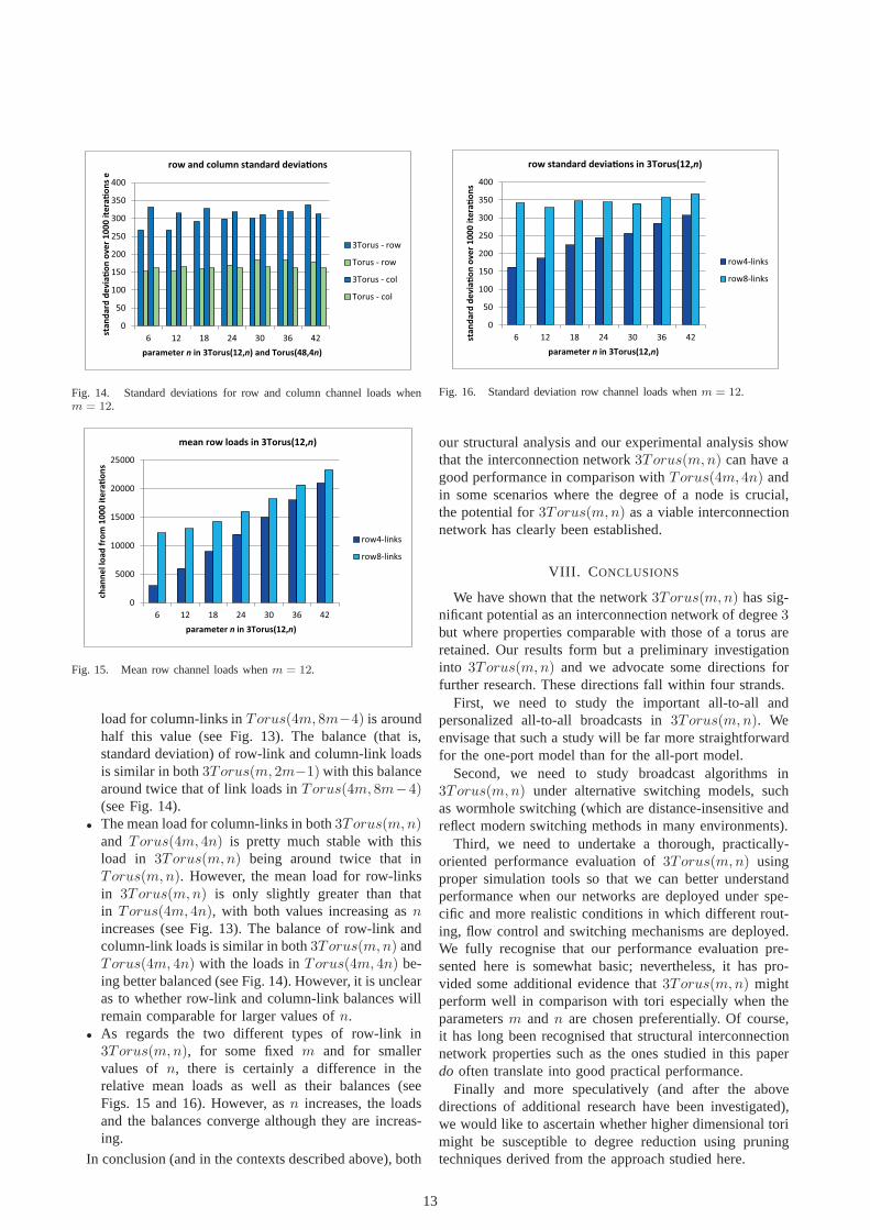
• The suspected ‘cusp’ scenario, whenn = 2m − 1,is indeed such with the mean load for row-links in3Torus(m, 2m−1) being almost identical to the meanload for column-links, as well as the mean load forrow-links in Torus(4m, 8m − 4); though the mean
12
0
50
100
150
200
250
300
350
400
6 12 18 24 30 36 42
sta
nd
ard
de
via
!o
n o
ve
r 1
00
0 i
tera
!o
ns
e
parameter n in 3Torus(12,n) and Torus(48,4n)
row and column standard devia!ons
3Torus - row
Torus - row
3Torus - col
Torus - col
Fig. 14. Standard deviations for row and column channel loads whenm = 12.
0
5000
10000
15000
20000
25000
6 12 18 24 30 36 42
cha
nn
el
loa
d f
rom
10
00
ite
ra!
on
s
parameter n in 3Torus(12,n)
mean row loads in 3Torus(12,n)
row4-links
row8-links
Fig. 15. Mean row channel loads whenm = 12.
load for column-links inTorus(4m, 8m−4) is aroundhalf this value (see Fig. 13). The balance (that is,standard deviation) of row-link and column-link loadsis similar in both3Torus(m, 2m−1) with this balancearound twice that of link loads inTorus(4m, 8m−4)(see Fig. 14).
• The mean load for column-links in both3Torus(m,n)and Torus(4m, 4n) is pretty much stable with thisload in 3Torus(m,n) being around twice that inTorus(m,n). However, the mean load for row-linksin 3Torus(m,n) is only slightly greater than thatin Torus(4m, 4n), with both values increasing asnincreases (see Fig. 13). The balance of row-link andcolumn-link loads is similar in both3Torus(m,n) andTorus(4m, 4n) with the loads inTorus(4m, 4n) be-ing better balanced (see Fig. 14). However, it is unclearas to whether row-link and column-link balances willremain comparable for larger values ofn.
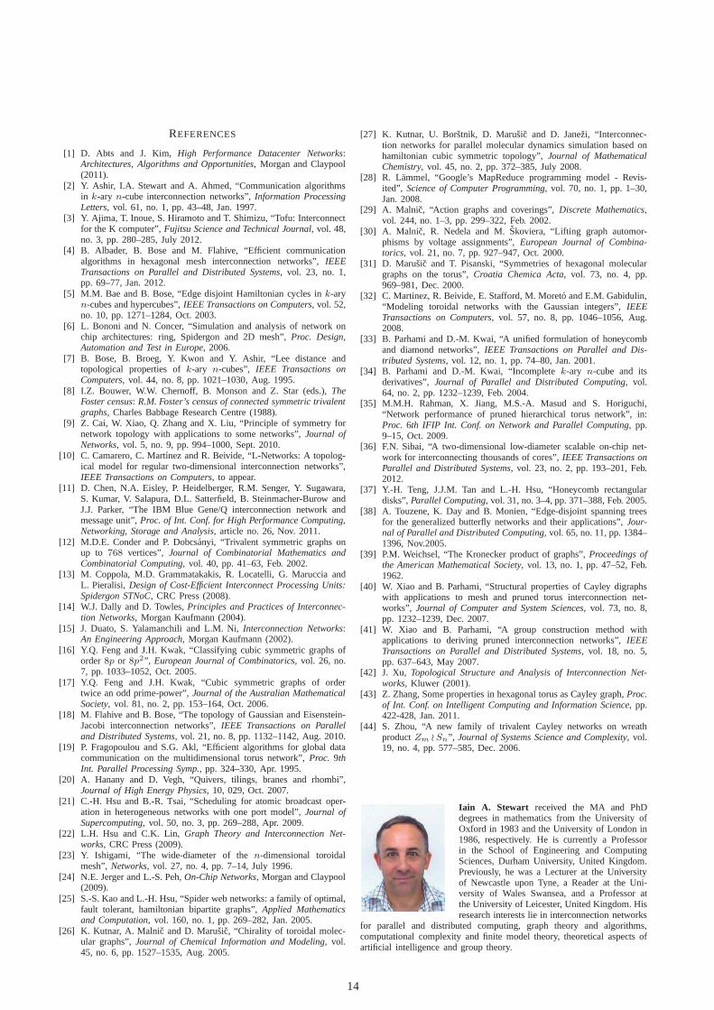
• As regards the two different types of row-link in3Torus(m,n), for some fixedm and for smallervalues of n, there is certainly a difference in therelative mean loads as well as their balances (seeFigs. 15 and 16). However, asn increases, the loadsand the balances converge although they are increas-ing.
In conclusion (and in the contexts described above), both
0
50
100
150
200
250
300
350
400
6 12 18 24 30 36 42sta
nd
ard
de
via
!o
n o
ve
r 1
00
0 i
tera
!o
ns
parameter n in 3Torus(12,n)
row standard devia!ons in 3Torus(12,n)
row4-links
row8-links
Fig. 16. Standard deviation row channel loads whenm = 12.
our structural analysis and our experimental analysis showthat the interconnection network3Torus(m,n) can have agood performance in comparison withTorus(4m, 4n) andin some scenarios where the degree of a node is crucial,the potential for3Torus(m,n) as a viable interconnectionnetwork has clearly been established.
VIII. C ONCLUSIONS
We have shown that the network3Torus(m,n) has sig-nificant potential as an interconnection network of degree3but where properties comparable with those of a torus areretained. Our results form but a preliminary investigationinto 3Torus(m,n) and we advocate some directions forfurther research. These directions fall within four strands.
First, we need to study the important all-to-all andpersonalized all-to-all broadcasts in3Torus(m,n). Weenvisage that such a study will be far more straightforwardfor the one-port model than for the all-port model.
Second, we need to study broadcast algorithms in3Torus(m,n) under alternative switching models, suchas wormhole switching (which are distance-insensitive andreflect modern switching methods in many environments).
Third, we need to undertake a thorough, practically-oriented performance evaluation of3Torus(m,n) usingproper simulation tools so that we can better understandperformance when our networks are deployed under spe-cific and more realistic conditions in which different rout-ing, flow control and switching mechanisms are deployed.We fully recognise that our performance evaluation pre-sented here is somewhat basic; nevertheless, it has pro-vided some additional evidence that3Torus(m,n) mightperform well in comparison with tori especially when theparametersm andn are chosen preferentially. Of course,it has long been recognised that structural interconnectionnetwork properties such as the ones studied in this paperdo often translate into good practical performance.
Finally and more speculatively (and after the abovedirections of additional research have been investigated),we would like to ascertain whether higher dimensional torimight be susceptible to degree reduction using pruningtechniques derived from the approach studied here.
13
REFERENCES
[1] D. Abts and J. Kim, High Performance Datacenter Networks:Architectures, Algorithms and Opportunities, Morgan and Claypool(2011).
[2] Y. Ashir, I.A. Stewart and A. Ahmed, “Communication algorithmsin k-ary n-cube interconnection networks”,Information ProcessingLetters, vol. 61, no. 1, pp. 43–48, Jan. 1997.
[3] Y. Ajima, T. Inoue, S. Hiramoto and T. Shimizu, “Tofu: Interconnectfor the K computer”,Fujitsu Science and Technical Journal, vol. 48,no. 3, pp. 280–285, July 2012.
[4] B. Albader, B. Bose and M. Flahive, “Efficient communicationalgorithms in hexagonal mesh interconnection networks”,IEEETransactions on Parallel and Distributed Systems, vol. 23, no. 1,pp. 69–77, Jan. 2012.
[5] M.M. Bae and B. Bose, “Edge disjoint Hamiltonian cycles in k-aryn-cubes and hypercubes”,IEEE Transactions on Computers, vol. 52,no. 10, pp. 1271–1284, Oct. 2003.
[6] L. Bononi and N. Concer, “Simulation and analysis of network onchip architectures: ring, Spidergon and 2D mesh”,Proc. Design,Automation and Test in Europe, 2006.
[7] B. Bose, B. Broeg, Y. Kwon and Y. Ashir, “Lee distance andtopological properties ofk-ary n-cubes”, IEEE Transactions onComputers, vol. 44, no. 8, pp. 1021–1030, Aug. 1995.
[8] I.Z. Bouwer, W.W. Chernoff, B. Monson and Z. Star (eds.),TheFoster census: R.M. Foster’s census of connected symmetric trivalentgraphs, Charles Babbage Research Centre (1988).
[9] Z. Cai, W. Xiao, Q. Zhang and X. Liu, “Principle of symmetry fornetwork topology with applications to some networks”,Journal ofNetworks, vol. 5, no. 9, pp. 994–1000, Sept. 2010.
[10] C. Camarero, C. Martınez and R. Beivide, “L-Networks:A topolog-ical model for regular two-dimensional interconnection networks”,IEEE Transactions on Computers, to appear.
[11] D. Chen, N.A. Eisley, P. Heidelberger, R.M. Senger, Y. Sugawara,S. Kumar, V. Salapura, D.L. Satterfield, B. Steinmacher-Burow andJ.J. Parker, “The IBM Blue Gene/Q interconnection network andmessage unit”,Proc. of Int. Conf. for High Performance Computing,Networking, Storage and Analysis, article no. 26, Nov. 2011.
[12] M.D.E. Conder and P. Dobcsanyi, “Trivalent symmetricgraphs onup to 768 vertices”, Journal of Combinatorial Mathematics andCombinatorial Computing, vol. 40, pp. 41–63, Feb. 2002.
[13] M. Coppola, M.D. Grammatakakis, R. Locatelli, G. Maruccia andL. Pieralisi, Design of Cost-Efficient Interconnect Processing Units:Spidergon STNoC, CRC Press (2008).
[14] W.J. Dally and D. Towles,Principles and Practices of Interconnec-tion Networks, Morgan Kaufmann (2004).
[15] J. Duato, S. Yalamanchili and L.M. Ni,Interconnection Networks:An Engineering Approach, Morgan Kaufmann (2002).
[16] Y.Q. Feng and J.H. Kwak, “Classifying cubic symmetric graphs oforder8p or 8p2”, European Journal of Combinatorics, vol. 26, no.7, pp. 1033–1052, Oct. 2005.
[17] Y.Q. Feng and J.H. Kwak, “Cubic symmetric graphs of ordertwice an odd prime-power”,Journal of the Australian MathematicalSociety, vol. 81, no. 2, pp. 153–164, Oct. 2006.
[18] M. Flahive and B. Bose, “The topology of Gaussian and Eisenstein-Jacobi interconnection networks”,IEEE Transactions on Paralleland Distributed Systems, vol. 21, no. 8, pp. 1132–1142, Aug. 2010.
[19] P. Fragopoulou and S.G. Akl, “Efficient algorithms for global datacommunication on the multidimensional torus network”,Proc. 9thInt. Parallel Processing Symp., pp. 324–330, Apr. 1995.
[20] A. Hanany and D. Vegh, “Quivers, tilings, branes and rhombi”,Journal of High Energy Physics, 10, 029, Oct. 2007.
[21] C.-H. Hsu and B.-R. Tsai, “Scheduling for atomic broadcast oper-ation in heterogeneous networks with one port model”,Journal ofSupercomputing, vol. 50, no. 3, pp. 269–288, Apr. 2009.
[22] L.H. Hsu and C.K. Lin,Graph Theory and Interconnection Net-works, CRC Press (2009).
[23] Y. Ishigami, “The wide-diameter of then-dimensional toroidalmesh”,Networks, vol. 27, no. 4, pp. 7–14, July 1996.
[24] N.E. Jerger and L.-S. Peh,On-Chip Networks, Morgan and Claypool(2009).
[25] S.-S. Kao and L.-H. Hsu, “Spider web networks: a family of optimal,fault tolerant, hamiltonian bipartite graphs”,Applied Mathematicsand Computation, vol. 160, no. 1, pp. 269–282, Jan. 2005.
[26] K. Kutnar, A. Malnic and D. Marusic, “Chirality of toroidal molec-ular graphs”,Journal of Chemical Information and Modeling, vol.45, no. 6, pp. 1527–1535, Aug. 2005.
[27] K. Kutnar, U. Borstnik, D. Marusic and D. Janezi, “Interconnec-tion networks for parallel molecular dynamics simulation based onhamiltonian cubic symmetric topology”,Journal of MathematicalChemistry, vol. 45, no. 2, pp. 372–385, July 2008.
[28] R. Lammel, “Google’s MapReduce programming model - Revis-ited”, Science of Computer Programming, vol. 70, no. 1, pp. 1–30,Jan. 2008.
[29] A. Malnic, “Action graphs and coverings”,Discrete Mathematics,vol. 244, no. 1–3, pp. 299–322, Feb. 2002.
[30] A. Malnic, R. Nedela and M.Skoviera, “Lifting graph automor-phisms by voltage assignments”,European Journal of Combina-torics, vol. 21, no. 7, pp. 927–947, Oct. 2000.
[31] D. Marusic and T. Pisanski, “Symmetries of hexagonalmoleculargraphs on the torus”,Croatia Chemica Acta, vol. 73, no. 4, pp.969–981, Dec. 2000.
[32] C. Martinez, R. Beivide, E. Stafford, M. Moreto and E.M. Gabidulin,“Modeling toroidal networks with the Gaussian integers”,IEEETransactions on Computers, vol. 57, no. 8, pp. 1046–1056, Aug.2008.
[33] B. Parhami and D.-M. Kwai, “A unified formulation of honeycomband diamond networks”,IEEE Transactions on Parallel and Dis-tributed Systems, vol. 12, no. 1, pp. 74–80, Jan. 2001.
[34] B. Parhami and D.-M. Kwai, “Incompletek-ary n-cube and itsderivatives”, Journal of Parallel and Distributed Computing, vol.64, no. 2, pp. 1232–1239, Feb. 2004.
[35] M.M.H. Rahman, X. Jiang, M.S.-A. Masud and S. Horiguchi,“Network performance of pruned hierarchical torus network”, in:Proc. 6th IFIP Int. Conf. on Network and Parallel Computing, pp.9–15, Oct. 2009.
[36] F.N. Sibai, “A two-dimensional low-diameter scalableon-chip net-work for interconnecting thousands of cores”,IEEE Transactions onParallel and Distributed Systems, vol. 23, no. 2, pp. 193–201, Feb.2012.
[37] Y.-H. Teng, J.J.M. Tan and L.-H. Hsu, “Honeycomb rectangulardisks”,Parallel Computing, vol. 31, no. 3–4, pp. 371–388, Feb. 2005.
[38] A. Touzene, K. Day and B. Monien, “Edge-disjoint spanning treesfor the generalized butterfly networks and their applications”, Jour-nal of Parallel and Distributed Computing, vol. 65, no. 11, pp. 1384–1396, Nov.2005.
[39] P.M. Weichsel, “The Kronecker product of graphs”,Proceedings ofthe American Mathematical Society, vol. 13, no. 1, pp. 47–52, Feb.1962.
[40] W. Xiao and B. Parhami, “Structural properties of Cayley digraphswith applications to mesh and pruned torus interconnectionnet-works”, Journal of Computer and System Sciences, vol. 73, no. 8,pp. 1232–1239, Dec. 2007.
[41] W. Xiao and B. Parhami, “A group construction method withapplications to deriving pruned interconnection networks”, IEEETransactions on Parallel and Distributed Systems, vol. 18, no. 5,pp. 637–643, May 2007.
[42] J. Xu, Topological Structure and Analysis of Interconnection Net-works, Kluwer (2001).
[43] Z. Zhang, Some properties in hexagonal torus as Cayley graph,Proc.of Int. Conf. on Intelligent Computing and Information Science, pp.422-428, Jan. 2011.
[44] S. Zhou, “A new family of trivalent Cayley networks on wreathproductZm ≀Sn”, Journal of Systems Science and Complexity, vol.19, no. 4, pp. 577–585, Dec. 2006.
Iain A. Stewart received the MA and PhDdegrees in mathematics from the University ofOxford in 1983 and the University of London in1986, respectively. He is currently a Professorin the School of Engineering and ComputingSciences, Durham University, United Kingdom.Previously, he was a Lecturer at the Universityof Newcastle upon Tyne, a Reader at the Uni-versity of Wales Swansea, and a Professor atthe University of Leicester, United Kingdom. Hisresearch interests lie in interconnection networks
for parallel and distributed computing, graph theory and algorithms,computational complexity and finite model theory, theoretical aspects ofartificial intelligence and group theory.
14