Interactive Procedural Modelling of Coherent Waterfall … · Interactive Procedural Modelling of Coherent Waterfall Scenes ... Computer Graphics Forum, Wiley, 2015 ... scene contains

HAL Id: hal-01095858https://hal.inria.fr/hal-01095858

Submitted on 8 Sep 2015

HAL is a multi-disciplinary open accessarchive for the deposit and dissemination of sci-entific research documents, whether they are pub-lished or not. The documents may come fromteaching and research institutions in France orabroad, or from public or private research centers.

L’archive ouverte pluridisciplinaire HAL, estdestinée au dépôt et à la diffusion de documentsscientifiques de niveau recherche, publiés ou non,émanant des établissements d’enseignement et derecherche français ou étrangers, des laboratoirespublics ou privés.

Interactive Procedural Modelling of Coherent WaterfallScenes

Arnaud Emilien, Pierre Poulin, Marie-Paule Cani, Ulysse Vimont

To cite this version:Arnaud Emilien, Pierre Poulin, Marie-Paule Cani, Ulysse Vimont. Interactive Procedural Mod-elling of Coherent Waterfall Scenes. Computer Graphics Forum, Wiley, 2015, 34 (6), pp.22-35.<10.1111/cgf.12515>. <hal-01095858>

https://hal.inria.fr/hal-01095858

https://hal.archives-ouvertes.fr

Volume xx (200y), Number z, pp. 1–15

Interactive Procedural Modeling of

Coherent Waterfall Scenes

A. Emilien1,2† P. Poulin1‡ M.-P. Cani2§ U. Vimont2¶

1 LIGUM, Dept. I.R.O., Université de Montréal 2 LJK, Université Grenoble-Alpes, CNRS & Inria

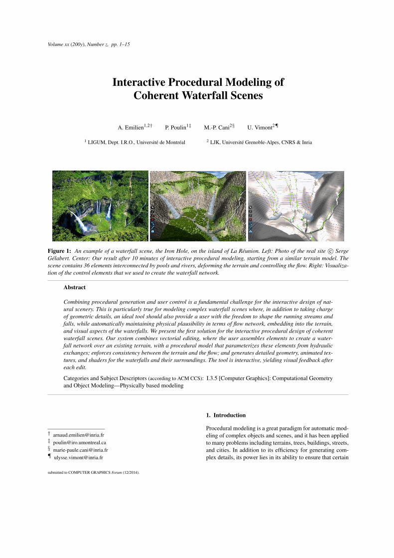
Figure 1: An example of a waterfall scene, the Iron Hole, on the island of La Réunion. Left: Photo of the real site c© Serge

Gélabert. Center: Our result after 10 minutes of interactive procedural modeling, starting from a similar terrain model. The

scene contains 36 elements interconnected by pools and rivers, deforming the terrain and controlling the flow. Right: Visualiza-

tion of the control elements that we used to create the waterfall network.

Abstract

Combining procedural generation and user control is a fundamental challenge for the interactive design of nat-

ural scenery. This is particularly true for modeling complex waterfall scenes where, in addition to taking charge

of geometric details, an ideal tool should also provide a user with the freedom to shape the running streams and

falls, while automatically maintaining physical plausibility in terms of flow network, embedding into the terrain,

and visual aspects of the waterfalls. We present the first solution for the interactive procedural design of coherent

waterfall scenes. Our system combines vectorial editing, where the user assembles elements to create a water-

fall network over an existing terrain, with a procedural model that parameterizes these elements from hydraulic

exchanges; enforces consistency between the terrain and the flow; and generates detailed geometry, animated tex-

tures, and shaders for the waterfalls and their surroundings. The tool is interactive, yielding visual feedback after

each edit.

Categories and Subject Descriptors (according to ACM CCS): I.3.5 [Computer Graphics]: Computational Geometryand Object Modeling—Physically based modeling

† [email protected]‡ [email protected]§ [email protected]¶ [email protected]

1. Introduction

Procedural modeling is a great paradigm for automatic mod-eling of complex objects and scenes, and it has been appliedto many problems including terrains, trees, buildings, streets,and cities. In addition to its efficiency for generating com-plex details, its power lies in its ability to ensure that certain

submitted to COMPUTER GRAPHICS Forum (12/2014).

2 A. Emilien, P. Poulin, M.-P. Cani, and U. Vimont / Interactive Procedural Modeling of Coherent Waterfall Scenes

constraints are respected (for instance from a physical, bi-ological, or architectural viewpoint), making it much easierfor the user to create plausible models.

However, when one has a very specific goal in mind, con-trolling the many intricate parameters of these automaticprocedures can be very cumbersome. In such situations, itwould be great to have access to an interactive system en-abling the user to handle the coarse design, while the systemautomatically ensures consistency and support for the proce-dural generation of all the details. In this paper, we apply thisparadigm of interconnected procedural generation and inter-active user-control, to the difficult task of modeling coherentwaterfall scenes.

Waterfalls offer some of the most beautiful settings in na-ture. Despite this, no easy-to-use method for designing wa-terfall scenes has been developed so far in computer graph-ics. One solution consists of using physically based simu-lation of fluids on top of a modified terrain. Unfortunately,modeling a terrain in order to produce specific waterfallsis an extremely daunting task. Fluid simulation depends onslopes, collisions, riverbeds, source influx, water properties,flow speed, etc. All the work of deforming a terrain doesnot ensure the final appearance of a waterfall, as these mutu-ally dependent constraints and the governing physical lawsare complex and highly nonlinear. Another potential solutionconsists of manually creating a few waterfalls with standardmodeling tools, using manifold meshes and/or particles, andthen positioning them along the terrain and connecting themby streams. In this long and tedious process, the artist alsoneeds to manually maintain the consistency between the ter-rain and waterfalls, as well as the self-consistency of the wa-terfall network.

In this paper, we combine interactive and proceduralmethods to enable fast and easy design of plausible water-fall scenes. Our solution, based on a new interactive proce-dural model for flowing-water networks, allows users to eas-ily shape complex waterfall scenes while automatically en-forcing the physical consistency of the results, both in termsof hydraulic flow and of plausible embedding into the ter-rain. Coherence is enforced at several levels, ensuring thatthe flow always goes downstream, the user-edited water net-work follows the terrain (or the terrain is adapted to the net-work), the flow is distributed in the network without loss orgain of volume, and that the type of waterfall and the appear-ance of water is adapted to the flow. Our main contributionsinclude:

• a slope-flow diagram-based classification of waterfalls;• three parametric models for designing waterfall elements;• a procedural method for ensuring waterfall network con-

sistency;• automatic methods for locally adapting user-input water

trajectories to the terrain and/or the terrain to the flow.

All these contributions combine into a framework allowing

an artistic approach to river and waterfall design. The result-ing scene could either be used as a synthetic environmentfor games or films, or as an initial setup for further refine-ment through physically based fluid simulation when moresophisticated simulation effects are needed.

2. Previous Work

Many types of procedural methods [STBB14] have beendesigned for specific types of objects, including ter-rains [GGG∗13], plants [LRBP12], buildings [LWW08],cities [CEW∗08], road networks [GPGB11], and vil-lages [EBP∗12]. To our knowledge, no previous work ad-dresses the procedural modeling of waterfall scenes. Wetherefore focus our literature review on the modeling ofrivers, waterfalls, and terrains, which are key elements forour problem.

2.1. Rivers and Waterfalls

Most previous methods for creating running-water elements,from rivers to waterfalls, consist in simulating shallow wa-ter flows over an existing terrain [KM90, HW04, KW06,TMFSG07, YNBH09, LH10, BSW10, CM10]. In particular,particle systems are heavily used for generating waterfalls.However, even when optimized with hierarchical or screen-space methods [BSW10], these approaches suffer from theinherent complexity of simulating networks of running waterover large environments. Moreover, they only provide indi-rect control on the nature of waterfalls and on the trajectoriesof streams, the latter being dictated by the geometry of theunderlying terrain.

To increase user control over complex waterfalls, Sak-aguchi et al. [SDZ∗07] introduce pre-tuned particle systemsdesigned to capture specific types of waterfalls. These sys-tems are assembled by the user to generate visually complexscenes. Another solution [GCZ∗06] directly creates water-fall scenes by placing polygonal primitives over the terrain,and renders them using animated textures. However, in bothcases, the consistency within the flow network and betweenthe terrain and waterfall elements needs to be manually en-sured by the user.

As with these two last approaches, we move away frompure simulation methods in order to give more control to theuser. However, we do so while maintaining the main benefitsof physically based simulation, namely automatically ensur-ing a coherent result. This includes both that flow strengthsare coherent between the elements of the waterfall networkand that each flow segment is geometrically consistent withrespect to the underlying terrain. The way our user-designedvector elements control flow trajectories is similar in spiritto the sketch-based approach from Bhat et al. [BSHK04] forediting videos of 2D flows, although their method is basedon video processing only and does not address the problemof plausibly embedding water flows into a 3D terrain.


A. Emilien, P. Poulin, M.-P. Cani, and U. Vimont / Interactive Procedural Modeling of Coherent Waterfall Scenes 3

Although we do not use their simulation methods, werely on rendering techniques introduced in previous workto display the aspects of waterfall scenes in real time: Yuet al. [YNBH09] derive an animated texture from the mo-tion of particles simulated at the surface of a river, which ef-fectively provides the appearance of a complex fluid. Thesetextures can be augmented with their flow skirting aroundstones and borders [YNS11]. Instead, Van Hoesel [vH11]tiles flow textures and modulates their application on the wa-ter surface polygons according to the flow speed. His methodproves to be quite efficient, compact, and effective. Zhu etal. [ZIH∗11] introduce an interactive flow and diffusion edi-tor with a sketching interface. The flow textures we use com-bine ideas from all of these approaches, and are enhancedby simple forms of particle systems, inspired by work fromHolmberg and Wünsche [HW04].

2.2. Terrains

Allowing users to design a specific waterfall scene oversome input terrain requires automatic ways of adapting theterrain in order to ensure consistency with the flow. Wetherefore briefly review previous methods for terrain gen-eration and editing.

Most terrain models are represented using a 2.5D height-field that is well adapted to GPU processing, enabling thehandling of very large environments [LH04, BN08]. In con-trast, Peytavie et al. [PGGM09] introduce a specific pilingmodel for capturing complex terrain structures, such as over-hangs and caves that can be observed at the top of free-fallsor near pools at their bottom. In our work, we instead adapta horizontal displacement method [GM01] to capture over-hangs over a standard heightfield representation.

Many solutions exist for terrain generation and edit-ing [SDKT∗09], from fully procedural methods to thosecombining examples or textures with sketch-based interac-tion. We focus on the latter, since they could be adapted tocontrol some local deformations of the terrain.

Hydraulic erosion methods [BTHB06,MDH07,ŠBBK08]simulate the effect of water flows on the progressive sculpt-ing of terrains, which results in very realistic landscapes.However, here the control is indirect since the flow dependson the current terrain. Therefore, this approach is not suit-able for our problem. Closer to our concerns, Génevaux etal. [GGG∗13] present a procedural method for generatingterrains based on hydrology: a realistic terrain is fully gen-erated from dense hydraulic graphs. Unfortunately, their ap-proach does not directly address our goal: we are insteadlooking for plausible ways to locally edit an existing terrainin order to make it consistent with user-designed flow net-works.

Re-using existing terrains to match user specifications,such as sketches, is generally accomplished using texture-based approaches, where heightfield patches from the input

terrain are combined to match user constraints [ZSTR07,TGM13]. We are rather interested in local, feature-basedediting of the input terrain, to have it match the range ofslopes and local geometry consistently with user-designedflow networks. We are therefore inspired by feature-basedterrain generation methods [HGA∗10, BMV∗11, GMS09],and we adapt them for the first time to the editing of an ex-isting heightfield.

3. Overview of our Method

The key goal of our method is to leave coarse design of wa-terfall scenes in the hands of the user, while providing auto-matic ways to generate plausible and detailed results.

In the real world, flow networks formed by complex wa-terfalls, such as the one in Figure 1(left), include free-falls,segments where running water remains in contact with theterrain, as well as pools. Moreover, each of these segmentscan be of many different types, from rivers to rapids forthe ones in contact with the terrain, and from plunges tocataracts for free-falls. Having to manually select plausibletypes for each segment of a full network would be both te-dious and require specialized knowledge from the user.

Below we propose a two-level classification for segmentsof waterfall networks, enabling us to leave the choice of low-level classes to the user, while automatically computing themost appropriate running-water types from quantitative in-formation, such as the slope of the underlying terrain andthe intensity of the flow. The processing pipeline that we usefor modeling a waterfall scene, based on this analysis, is pre-sented next.

3.1. Two-level Classification for Running Water

Waterfall scenes are comprised of three types of elements:running-water segments that remain in contact with the ter-rain, free-fall segments where water is in the air, and poolsthat receive water from the free-falls. Our goal is to providesome coarse, intuitive control to the user, and we leave thechoice of these three classes, contact, free-fall, and pool, tothe user during interactive design.

In contrast, we would like to free the user from the manualand explicit determination of the precise characteristics thateach running-water segment should take, because this can bedetermined in a more plausible way using an automatic pro-cedure. After studying the existing classifications of streamsand falls, we designed a new, slope-flow classification thatmatches our goals, as explained next.

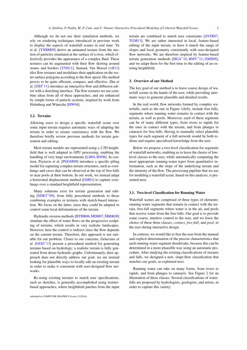
Running water can take on many forms, from rivers torapids, and from plunges to cataracts. See Figure 2 for anillustration of these classes. Several classifications of water-falls are proposed by hydrologists, geologists, and artists, inorder to capture this variety:



stream river rapid cascade horsetail block cataract ledge plunge ribbon

Figure 2: Artistic drawings illustrating the different types of running water and free-falls that can be found in nature.

• volume-based classifications of waterfalls [Bei06] sortwaterfalls into classes by using a logarithmic scale overthe volume of water in the air at a given time. Althougheasy to compute from quantitative information, this clas-sification provides little clue on the visual aspect of thefall. Moreover, it is restricted to free-falls, and thereforedoes not fully meet our needs;

• geometric classifications, such as the one found in the Wa-terfall Lover’s Guides [DD06, Plu05] or the one depictedin Figure 2, analyze the different types of geometries thatcan be observed in nature. However, they only providevisual information. No quantitative measurement is pro-posed to automatically compute the class that a running-water segment belongs to.

In this work, we would like to classify waterfall segmentsfrom quantitative information, while getting visual clues en-abling us to generate plausible 3D representations for eachsegment. We therefore decided to augment the geometricclassification of Figure 2 with quantitative evaluation of theclasses, as in volume-based approaches. However, we needmeasures applicable to both running water in contact withthe terrain and to free-falls, and therefore our solution is dif-ferent.

By studying the existing geometric classifications andlooking at many real cases, we noticed that the geomet-ric type of running water mostly depends on two importantquantitative parameters: the flow value (defined as the vol-ume of water per second traveling through a cross-section ofthe segment), and the local slope of the terrain. Intuitively,when the flow decreases, a river becomes a stream, a cas-cade becomes a horsetail, and a free-fall cataract becomesa ledge. Meanwhile, if a given water flow is running on ter-rains of increasing slope, a river tends to become a rapid, andthen eventually a block.

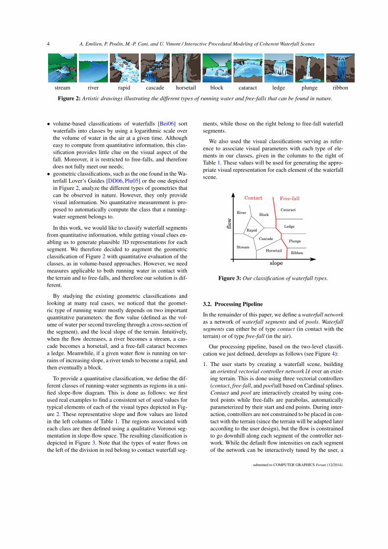
To provide a quantitative classification, we define the dif-ferent classes of running-water segments as regions in a uni-fied slope-flow diagram. This is done as follows: we firstused real examples to find a consistent set of seed values fortypical elements of each of the visual types depicted in Fig-ure 2. These representative slope and flow values are listedin the left columns of Table 1. The regions associated witheach class are then defined using a qualitative Voronoi seg-mentation in slope-flow space. The resulting classification isdepicted in Figure 3. Note that the types of water flows onthe left of the division in red belong to contact waterfall seg-

ments, while those on the right belong to free-fall waterfallsegments.

We also used the visual classifications serving as refer-ence to associate visual parameters with each type of ele-ments in our classes, given in the columns to the right ofTable 1. These values will be used for generating the appro-priate visual representation for each element of the waterfallscene.

slope

Contact Free-fall

Stream

River

Rapid

Cascade

Horsetail

Cataract

Ledge

Plunge

Ribbon

Block

flow

Figure 3: Our classification of waterfall types.

3.2. Processing Pipeline

In the remainder of this paper, we define a waterfall network

as a network of waterfall segments and of pools. Waterfall

segments can either be of type contact (in contact with theterrain) or of type free-fall (in the air).

Our processing pipeline, based on the two-level classifi-cation we just defined, develops as follows (see Figure 4):

1. The user starts by creating a waterfall scene, buildingan oriented vectorial controller network U over an exist-ing terrain. This is done using three vectorial controllers(contact, free-fall, and pool)all based on Cardinal splines.Contact and pool are interactively created by using con-trol points while free-falls are parabolas, automaticallyparameterized by their start and end points. During inter-action, controllers are not constrained to be placed in con-tact with the terrain (since the terrain will be adapted lateraccording to the user design), but the flow is constrainedto go downhill along each segment of the controller net-work. While the default flow intensities on each segmentof the network can be interactively tuned by the user, a



Type Slope Flow Foam Rocks Dist. Part.

Ribbon π/2 1 0 0.3 0 0Plunge π/2 2 1 0.4 0 0.2Ledge π/2 5 0 0.5 0 0.5

Cataract π/2 8 1 1 1 1Stream π/16 2 0 0.2 0 0River π/32 5 0 0.2 0.1 0Rapid π/16 5 0.2 0.5 0.5 0

Cascade π/8 3 0.5 1 1 0Horsetail π/4 2 1 0 0 0

Block π/4 6 1 0 0.2 0

Table 1: Classification of running-water segments that may

appear in a waterfall network. The coordinates (slope, flow)

give the position of the class seed in the slope-flow dia-

gram of Figure 3. Slope is an average inclination in radi-

ans, while flow is expressed in “flow units”, which gives

an informal notion of relative proportions between waterfall

types. Foam, rocks, disturbance, and particle are parameters

(∈ [0,1]) used in our procedural generation of geometry and

for rendering.

consistent hydraulic graph G (with fully consistent flowvalues) is automatically computed at the end of the inter-active modeling process. (See Section 4)

2. The next step is the generation of the waterfall net-

work W , which uses the coarse water trajectories fromthe controller network and the flow information from thehydraulic graph to define a more precise representationof the waterfall. In addition to directly using the controlcurves that they defined, the user has the option of furtherrefining the geometry of the network through an auto-matic procedure that locally adapts running-water trajec-tories to the underlying terrain. Each curve of the networkis then divided into a number of water segments, whosesub-class is determined by slope-flow classification fromSection 3.1. Finally, the last geometric parameters, suchas flow width and depth, are computed for each segmentof the waterfall network. (See Section 5)

3. Lastly, the 3D representation for the waterfall network,called the integration mesh, is generated and embeddedinto the scene through appropriate local deformations ofthe terrain. Although they can include large changes, suchas digging a canyon to allow a stream to find its waydownhill (in the extreme case where the user designedwater segments go through a mountain), constraints ap-plied to the terrain are mainly aimed at automaticallyadding all the details that make the scene plausible: thisincludes borders along streams, riverbeds, and the cre-ation of overhangs behind free-falls. Appropriate deco-rative elements such as trees and rocks are generated atthis stage, using the distance to the closest riverbed andthe class of the waterfall segment it belongs to as de-

Figure 4: Processing pipeline used for creating waterfall

scenes. The first step is the creation by the artist of the con-

troller network U . Then, a hydraulic graph G is generated;

the width of an arc encodes flow quantity. The waterfall net-

work W is then generated with a subdivision algorithm, and

the waterfall types are determined. Finally, the integration

mesh M is generated and used to deform the terrain and

generate the procedural details.

sign guidelines. Rendering attributes are also set from theclass of each segment. (See Section 6)

Note that we chose to compute a coherent hydraulicgraph G (Step 1 of the pipeline above) based on the con-troller network U , i.e., from the coarse trajectories definedby the user, before refining these trajectories into a water-fall network W . This enables us to use consistent flow val-ues in Step 2, while refining water trajectories. This helpsus, for instance, to prevent large rivers from being refinedinto a series of short twists when adapted to the terrain, al-though a smaller stream would be allowed to be more wind-ing. The fact that our algorithm interleaves geometric com-



p

p

j,k-1

j,k

smin

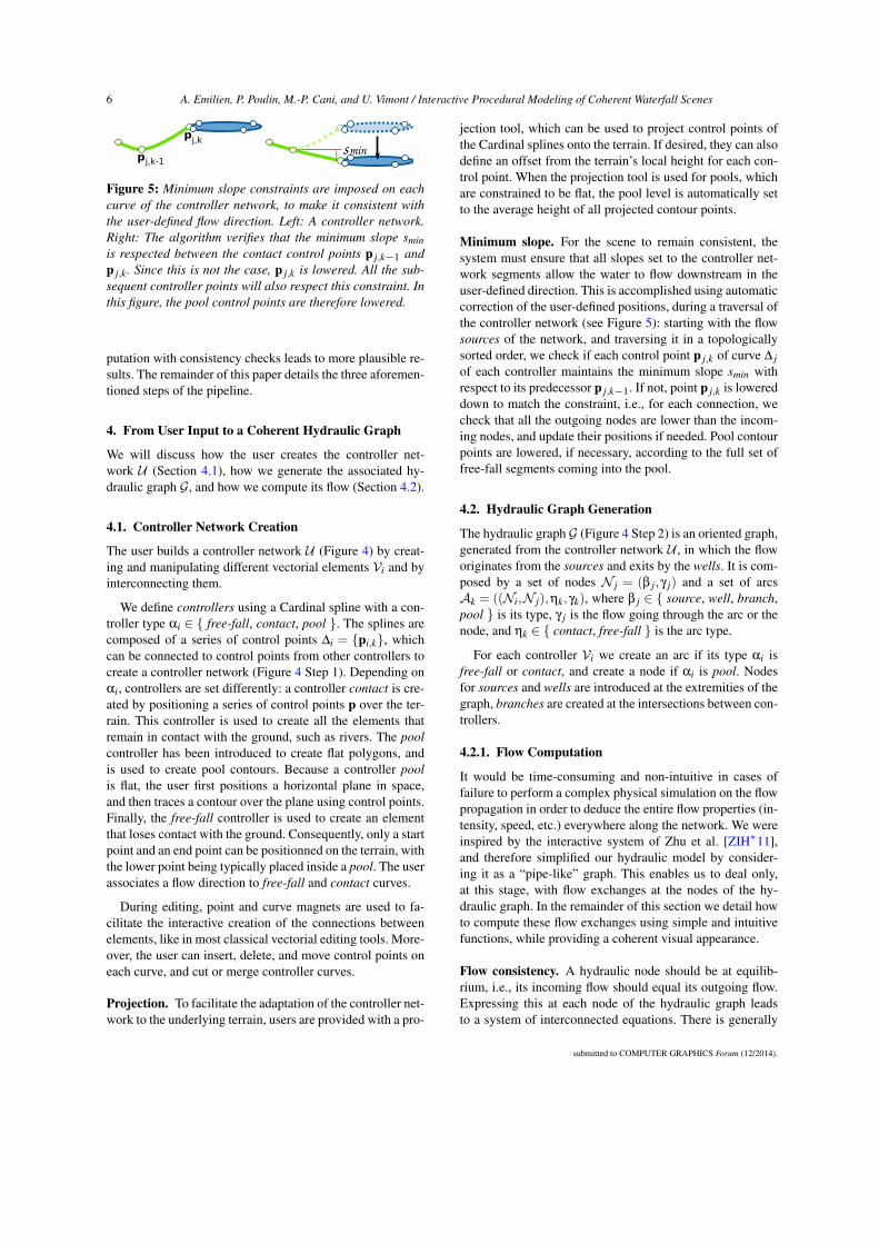
Figure 5: Minimum slope constraints are imposed on each

curve of the controller network, to make it consistent with

the user-defined flow direction. Left: A controller network.

Right: The algorithm verifies that the minimum slope smin

is respected between the contact control points p j,k−1 and

p j,k. Since this is not the case, p j,k is lowered. All the sub-

sequent controller points will also respect this constraint. In

this figure, the pool control points are therefore lowered.

putation with consistency checks leads to more plausible re-sults. The remainder of this paper details the three aforemen-tioned steps of the pipeline.

4. From User Input to a Coherent Hydraulic Graph

We will discuss how the user creates the controller net-work U (Section 4.1), how we generate the associated hy-draulic graph G, and how we compute its flow (Section 4.2).

4.1. Controller Network Creation

The user builds a controller network U (Figure 4) by creat-ing and manipulating different vectorial elements Vi and byinterconnecting them.

We define controllers using a Cardinal spline with a con-troller type αi ∈ free-fall, contact, pool . The splines arecomposed of a series of control points ∆i = pi,k, whichcan be connected to control points from other controllers tocreate a controller network (Figure 4 Step 1). Depending onαi, controllers are set differently: a controller contact is cre-ated by positioning a series of control points p over the ter-rain. This controller is used to create all the elements thatremain in contact with the ground, such as rivers. The pool

controller has been introduced to create flat polygons, andis used to create pool contours. Because a controller pool

is flat, the user first positions a horizontal plane in space,and then traces a contour over the plane using control points.Finally, the free-fall controller is used to create an elementthat loses contact with the ground. Consequently, only a startpoint and an end point can be positionned on the terrain, withthe lower point being typically placed inside a pool. The userassociates a flow direction to free-fall and contact curves.

During editing, point and curve magnets are used to fa-cilitate the interactive creation of the connections betweenelements, like in most classical vectorial editing tools. More-over, the user can insert, delete, and move control points oneach curve, and cut or merge controller curves.

Projection. To facilitate the adaptation of the controller net-work to the underlying terrain, users are provided with a pro-

jection tool, which can be used to project control points ofthe Cardinal splines onto the terrain. If desired, they can alsodefine an offset from the terrain’s local height for each con-trol point. When the projection tool is used for pools, whichare constrained to be flat, the pool level is automatically setto the average height of all projected contour points.

Minimum slope. For the scene to remain consistent, thesystem must ensure that all slopes set to the controller net-work segments allow the water to flow downstream in theuser-defined direction. This is accomplished using automaticcorrection of the user-defined positions, during a traversal ofthe controller network (see Figure 5): starting with the flowsources of the network, and traversing it in a topologicallysorted order, we check if each control point p j,k of curve ∆ j

of each controller maintains the minimum slope smin withrespect to its predecessor p j,k−1. If not, point p j,k is lowereddown to match the constraint, i.e., for each connection, wecheck that all the outgoing nodes are lower than the incom-ing nodes, and update their positions if needed. Pool contourpoints are lowered, if necessary, according to the full set offree-fall segments coming into the pool.

4.2. Hydraulic Graph Generation

The hydraulic graph G (Figure 4 Step 2) is an oriented graph,generated from the controller network U , in which the floworiginates from the sources and exits by the wells. It is com-posed by a set of nodes N j = (β j,γ j) and a set of arcsAk = ((Ni,N j),ηk,γk), where β j ∈ source, well, branch,pool is its type, γ j is the flow going through the arc or thenode, and ηk ∈ contact, free-fall is the arc type.

For each controller Vi we create an arc if its type αi isfree-fall or contact, and create a node if αi is pool. Nodesfor sources and wells are introduced at the extremities of thegraph, branches are created at the intersections between con-trollers.

4.2.1. Flow Computation

It would be time-consuming and non-intuitive in cases offailure to perform a complex physical simulation on the flowpropagation in order to deduce the entire flow properties (in-tensity, speed, etc.) everywhere along the network. We wereinspired by the interactive system of Zhu et al. [ZIH∗11],and therefore simplified our hydraulic model by consider-ing it as a “pipe-like” graph. This enables us to deal only,at this stage, with flow exchanges at the nodes of the hy-draulic graph. In the remainder of this section we detail howto compute these flow exchanges using simple and intuitivefunctions, while providing a coherent visual appearance.

Flow consistency. A hydraulic node should be at equilib-rium, i.e., its incoming flow should equal its outgoing flow.Expressing this at each node of the hydraulic graph leadsto a system of interconnected equations. There is generally



an infinite number of solutions to this system. Therefore, in-stead of using a global solver to find consistent flow values,we solve them in succession for each node of the graph, ex-ploring it in dependency order from sources to wells. Thisenables us to take into account the user specifications for therelative strength of the input flows, and to generate a solutionthat best matches the coarse geometric trajectories in termsof branching angles at each node. Our method for doing sois explained next.

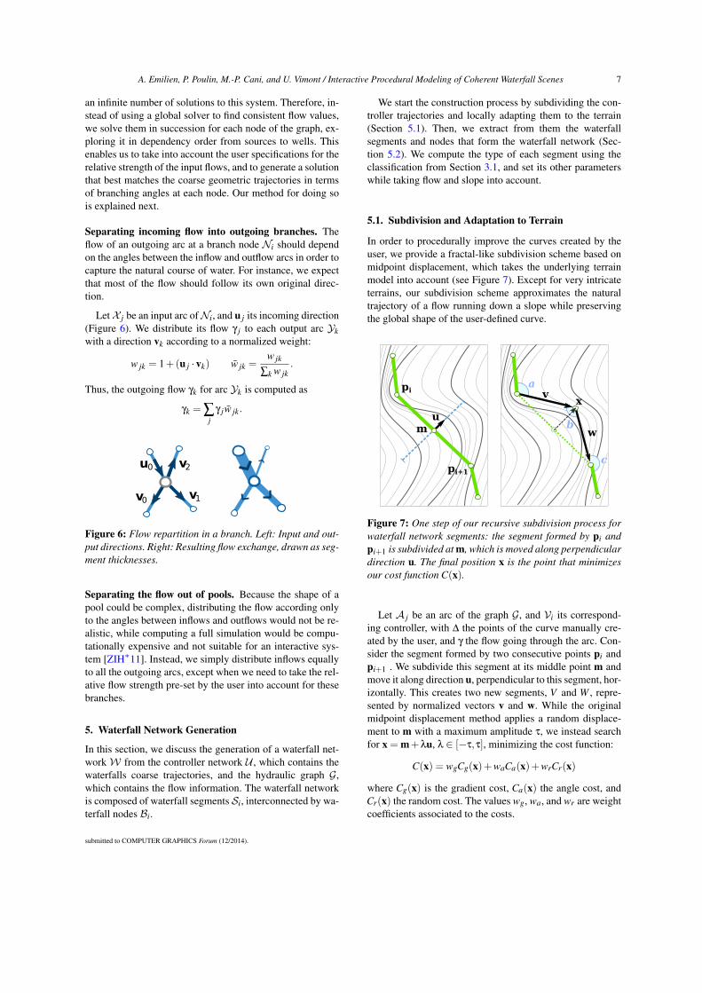
Separating incoming flow into outgoing branches. Theflow of an outgoing arc at a branch node Ni should dependon the angles between the inflow and outflow arcs in order tocapture the natural course of water. For instance, we expectthat most of the flow should follow its own original direc-tion.

Let X j be an input arc of Ni, and u j its incoming direction(Figure 6). We distribute its flow γ j to each output arc Yk

with a direction vk according to a normalized weight:

w jk = 1+(u j ·vk) w jk =w jk

∑k w jk

.

Thus, the outgoing flow γk for arc Yk is computed as

γk = ∑j

γ jw jk.

u v0 2

v0 v1

Figure 6: Flow repartition in a branch. Left: Input and out-

put directions. Right: Resulting flow exchange, drawn as seg-

ment thicknesses.

Separating the flow out of pools. Because the shape of apool could be complex, distributing the flow according onlyto the angles between inflows and outflows would not be re-alistic, while computing a full simulation would be compu-tationally expensive and not suitable for an interactive sys-tem [ZIH∗11]. Instead, we simply distribute inflows equallyto all the outgoing arcs, except when we need to take the rel-ative flow strength pre-set by the user into account for thesebranches.

5. Waterfall Network Generation

In this section, we discuss the generation of a waterfall net-work W from the controller network U , which contains thewaterfalls coarse trajectories, and the hydraulic graph G,which contains the flow information. The waterfall networkis composed of waterfall segments Si, interconnected by wa-terfall nodes Bi.

We start the construction process by subdividing the con-troller trajectories and locally adapting them to the terrain(Section 5.1). Then, we extract from them the waterfallsegments and nodes that form the waterfall network (Sec-tion 5.2). We compute the type of each segment using theclassification from Section 3.1, and set its other parameterswhile taking flow and slope into account.

5.1. Subdivision and Adaptation to Terrain

In order to procedurally improve the curves created by theuser, we provide a fractal-like subdivision scheme based onmidpoint displacement, which takes the underlying terrainmodel into account (see Figure 7). Except for very intricateterrains, our subdivision scheme approximates the naturaltrajectory of a flow running down a slope while preservingthe global shape of the user-defined curve.

um

xv

w

a

b

c

pi

pi+1

Figure 7: One step of our recursive subdivision process for

waterfall network segments: the segment formed by pi and

pi+1 is subdivided at m, which is moved along perpendicular

direction u. The final position x is the point that minimizes

our cost function C(x).

Let A j be an arc of the graph G, and Vi its correspond-ing controller, with ∆ the points of the curve manually cre-ated by the user, and γ the flow going through the arc. Con-sider the segment formed by two consecutive points pi andpi+1 . We subdivide this segment at its middle point m andmove it along direction u, perpendicular to this segment, hor-izontally. This creates two new segments, V and W , repre-sented by normalized vectors v and w. While the originalmidpoint displacement method applies a random displace-ment to m with a maximum amplitude τ, we instead searchfor x = m+λu, λ ∈ [−τ,τ], minimizing the cost function:

C(x) = wgCg(x)+waCa(x)+wrCr(x)

where Cg(x) is the gradient cost, Ca(x) the angle cost, andCr(x) the random cost. The values wg, wa, and wr are weightcoefficients associated to the costs.



Gradient cost. The gradient cost favors paths that followthe slope of the terrain, and is defined as:

Cg(x)=

∫V ‖g(t))‖ fp(v,g(t))dt+

∫W ‖g(t))‖ fp(w,g(t))dt

‖pi+1 −pi‖,

fp(v,g(t)) =

(

−2v ·g(t)

‖g(t)‖

)

+1,

where vector g(t) is the gradient of the terrain elevation atposition t. By integrating the elevation gradient along seg-ments V and W , and by using the scalar product betweenthe gradient and the segment vectors (v or w) as a penaltycoefficient, the path will follow the slope and avoid obsta-cles (Figure 7). Moreover, instead of simply using the scalarproduct value as a penality coefficient, we use function fp topenalize paths that follow the isolines (i.e., when the scalarproduct with the gradient is zero); climbing a slope is penal-ized even more severly. Consequently, this cost is low whenv and w are aligned in the same direction as the slope of theterrain, and high otherwise.

Angle cost. The angle cost prevents undesirable sharp an-gles that could appear between two consecutive segments,because of their independent subdivisions. We take into ac-count the angles a, b, and c (in radians), created at the intro-duction of new point x (see Figure 7), as:

Ca(x) =(

a

π

)2+

(

b

π

)2

+(

c

π

)2.

Random cost. Finally, to add fractal-like details on flat ter-rains, we use the random cost Cr(x), which is negligiblewhen the other costs are high.

The segments are recursively subdivided until their lengthis inferior to l. Displacement amplitude τ and detail size l

are set as:

τ = ‖u‖/2 l = γ/σ.

The minimum subdivision length l is proportional to the seg-ment flow, where σ is a user parameter. This enables us toget a more detailed trajectory for small flow values, enablingstreams to become more winding than rivers. In our proto-type we use the following values: σ= 1/2, wg = 1, wa = 0.1,and wr = 0.2 for all our examples.

5.2. Waterfall Network Construction

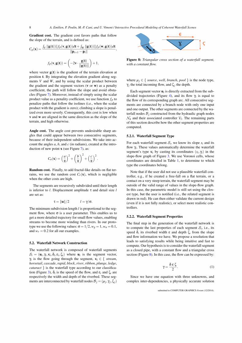
The waterfall network is composed of waterfall segmentsSi = (ui,γi,κi,δi,εi,ζi) where ui is the segment vector,γi is the flow going through the segment, κi ∈ stream,horsetail, cascade, rapid, block, river, ribbon, plunge, ledge,cataract is the waterfall type according to our classifica-tion (Figure 3), δi is the speed of the flow, and εi and ζi arerespectively the width and depth of the riverbed. These seg-ments are interconnected by waterfall nodes B j = (µ j,γ j,ζ j)

Figure 8: Triangular cross section of a waterfall segment,

with a constant flow.

where µ j ∈ source, well, branch, pool is the node type,γ j the total incoming flow, and ζ j the depth.

Each segment vector ui is directly extracted from the sub-divided trajectories (Figure 4), and its flow γi is equal tothe flow of its corresponding graph arc. All consecutive seg-ments are connected by a branch node with only one inputand one output. The other segments are connected by the wa-terfall nodes B j constructed from the hydraulic graph nodesNk and their associated controller Vl . The remaining partsof this section describe how the other segment properties arecomputed.

5.2.1. Waterfall Segment Type

For each waterfall segment Si, we know its slope si and itsflow γi. These values automatically determine the waterfallsegment’s type κi by casting its coordinates (si,γi) in theslope-flow graph of Figure 3. We use Voronoi cells, whosecoordinates are detailed in Table 1, to determine to whichtype the coordinates belong.

Note that if the user did not use a plausible waterfall con-troller, e.g., if he created a free-fall on a flat terrain, or acontact on a very steep terrain, the waterfall segment may beoutside of the valid range of values in the slope-flow graph.In this case, the parametric model is still set using the clos-est type, but the user is notified (i.e., the related segment isdrawn in red). He can then either validate the current design(even if it is not fully realistic), or select more realistic con-trollers.

5.2.2. Waterfall Segment Properties

The final step in the generation of the waterfall network isto compute the last properties of each segment Si, i.e., itsspeed δ, its riverbed width ε and depth ζ, from the slopeand flow information we have. We propose a resolution thatleads to satisfying results while being intuitive and fast tocompute. Our hypothesis is to consider the waterfall segmentas a closed pipe, with a constant flow and a triangular crosssection (Figure 8). In this case, the flow can be expressed by:

γ =δ ε ζ

2. (1)

Since we have one equation with three unknowns, andcomplex inter-dependencies, a physically accurate solution



should rely on strong assumptions, which cannot be justi-fied in our context. Instead, we decided to solve the systemby providing simple and intuitive functions to compute thesevariables.

We first propose to solve for the speed as a simple lin-ear function of slope s: δ = ks, k ∈ R

+. Then, we set thedepth as a function fd of the width and of the segment typeas: ζ = fd(ε,γ). Note that our slope constraint enforces thats > 0 everywhere for a waterfall segment. We used k = 10 inall our scenes. In our prototype, we use only one profile func-tion, fd(ε,γ) =

12 γ. Applying Equation (1), it is now possible

to compute the width and to deduce the depth value.

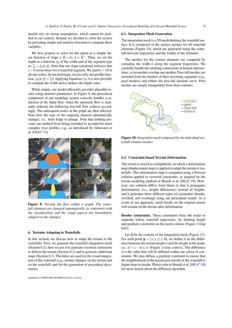
While simple, our model efficiently provides plausible re-sults using intuitive parameters. In Figure 9, the proceduralcomponent of our modeling system correctly handles a re-duction of the input flow: when the upstream flow is man-ually reduced, the following free-fall flow reduces accord-ingly. The subsequent nodes in the graph are then affected.Note how the type of the outgoing element automaticallychanges, i.e., from ledge to plunge. Note that nothing pre-vents our method from being extended to account for morecomplex river profiles, e.g., as introduced by Génevaux etal. [GGG∗13].

Figure 9: Varying the flow within a graph. The water-

fall elements are changed automatically, in conformity with

the classification, and the visual aspects are immediately

adapted to the changes.

6. Terrains Adapting to Waterfalls

In this section, we discuss how to adapt the terrain to thewaterfalls. First, we generate the waterfall integration mesh(Section 6.1), then we use it to generate vectorial constraintsto deform the terrain (Section 6.2) and to generate additionalmaps (Section 6.3). The latter are used for the visual integra-tion of the waterfall (e.g., texture changes on the terrain andon the waterfall) and for the generation of procedural deco-rations.

6.1. Integration Mesh Generation

The integration mesh is a 3D mesh defining the waterfall sur-face. It is composed of the surface meshes for all waterfallelements (Figure 10), which are generated using the water-fall network trajectories and the widths of the elements.

The meshes for the contact elements are computed byextruding the width ε along the segment trajectories. Wecarefully handle the meshing connections at branch intersec-tions, so no meshes overlap one another. Free-fall meshes areextruded from the borders of their incoming segments (e.g.,pool borders) and follow the free-fall element curve. Poolmeshes are simply triangulated from their contours.

contactpoolfree-fallbranch

Figure 10: Integration mesh composed by the individual wa-

terfall element meshes.

6.2. Constraint-based Terrain Deformation

The terrain is stored as a heightfield, on which a deformationmap (displacement map) is applied to adapt the terrain to wa-terfalls. This deformation map is computed using a Poissonsolution applied to vectorial constraints, as inspired by theterrain modeling method of Hnaidi et al. [HGA∗10]. How-ever, our solution differs from theirs in that it propagatesdeformations (i.e., height differences) instead of heights,and it generates three different types of constraints (border,riverbed, and overhang) using our procedural model. As aresult of our approach, small details on the original terrainwill remain on the terrain after deformation.

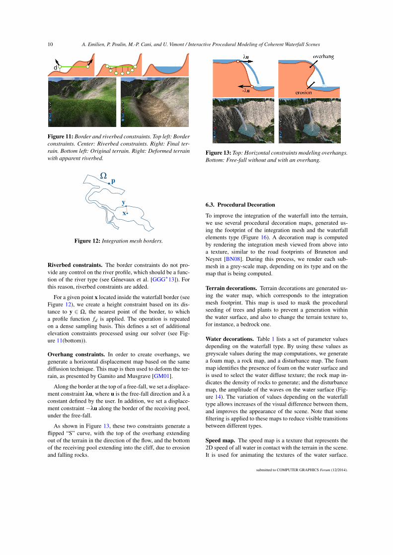
Border constraints. These constraints force the water tonaturally follow waterfall trajectories, by defining heightand gradient constraints on the mesh contour (Figure 11(topleft)).

Let Ω be the contour of the integration mesh (Figure 12).For each point p = (x,y,z) ∈ Ω, we define d as the differ-ence between the terrain height h and the height at the point,i.e., d = z− h(x,y) (Figure 11(top center)). The differenced is the value that will be diffused within our solver of con-straints. We also diffuse a gradient constraint to ensure thatthe neighborhood of the terrain just outside of the waterfall ishigher than its border. Please refer to Hnaidi et al. [HGA∗10]for more details about the diffusion algorithm.



d

Figure 11: Border and riverbed constraints. Top left: Border

constraints. Center: Riverbed constraints. Right: Final ter-

rain. Bottom left: Original terrain. Right: Deformed terrain

with apparent riverbed.

p

x

y

Figure 12: Integration mesh borders.

Riverbed constraints. The border constraints do not pro-vide any control on the river profile, which should be a func-tion of the river type (see Génevaux et al. [GGG∗13]). Forthis reason, riverbed constraints are added.

For a given point x located inside the waterfall border (seeFigure 12), we create a height constraint based on its dis-tance to y ∈ Ω, the nearest point of the border, to whicha profile function fd is applied. The operation is repeatedon a dense sampling basis. This defines a set of additionalelevation constraints processed using our solver (see Fig-ure 11(bottom)).

Overhang constraints. In order to create overhangs, wegenerate a horizontal displacement map based on the samediffusion technique. This map is then used to deform the ter-rain, as presented by Gamito and Musgrave [GM01].

Along the border at the top of a free-fall, we set a displace-ment constraint λu, where u is the free-fall direction and λ aconstant defined by the user. In addition, we set a displace-ment constraint −λu along the border of the receiving pool,under the free-fall.

As shown in Figure 13, these two constraints generate aflipped “S” curve, with the top of the overhang extendingout of the terrain in the direction of the flow, and the bottomof the receiving pool extending into the cliff, due to erosionand falling rocks.

Figure 13: Top: Horizontal constraints modeling overhangs.

Bottom: Free-fall without and with an overhang.

6.3. Procedural Decoration

To improve the integration of the waterfall into the terrain,we use several procedural decoration maps, generated us-ing the footprint of the integration mesh and the waterfallelements type (Figure 16). A decoration map is computedby rendering the integration mesh viewed from above intoa texture, similar to the road footprints of Bruneton andNeyret [BN08]. During this process, we render each sub-mesh in a grey-scale map, depending on its type and on themap that is being computed.

Terrain decorations. Terrain decorations are generated us-ing the water map, which corresponds to the integrationmesh footprint. This map is used to mask the proceduralseeding of trees and plants to prevent a generation withinthe water surface, and also to change the terrain texture to,for instance, a bedrock one.

Water decorations. Table 1 lists a set of parameter valuesdepending on the waterfall type. By using these values asgreyscale values during the map computations, we generatea foam map, a rock map, and a disturbance map. The foammap identifies the presence of foam on the water surface andis used to select the water diffuse texture; the rock map in-dicates the density of rocks to generate; and the disturbancemap, the amplitude of the waves on the water surface (Fig-ure 14). The variation of values depending on the waterfalltype allows increases of the visual difference between them,and improves the appearance of the scene. Note that somefiltering is applied to these maps to reduce visible transitionsbetween different types.

Speed map. The speed map is a texture that represents the2D speed of all water in contact with the terrain in the scene.It is used for animating the textures of the water surface.



Figure 14: Using the integration mesh and the waterfall types, we generate various maps used to render the waterfalls.

Figure 15 shows how the speed of the water is computed de-pending on the type of the segment. We use three differentapproaches to compute the surface speed of contacts, pools,and branches. For a contact, the speed at point x is given by

δx = δc

(

1− ‖x−c‖‖b−c‖

)

where c and b are the projections of

x along the cross section on the main axis and on the shorerespectively. For a pool, a fixed number of 2D fluid simu-lation steps [Sta99] are evaluated. For branches, we use 2Dinterpolation based on a standard technique of weighting bythe inverse distance, where each point pi is considered as avelocity constraint δi. The speed within a branch is given byδx = ∑i ωi δi. Interpolation weights ωi are computed usingthe equation:

ωi =ωi

∑i ωiωi = ∏

j

(

1−‖x−pi‖

‖p j −pi‖

)

.

Figure 15: Internal speed computation for a contact (left), a

pool (center), and a branch (right).

7. Implementation and Results

The system is implemented in C++, using OpenGL andGLSL Compute Shaders. The computations are performedon an NVidia 660GTX GPU and an Intel R© Xeon R© E5-1650CPU, running at 3.20 GHz with 16 GB of memory. The sys-tem uses two threads: one CPU thread for the interface andcomputation control, and one CPU/GPU thread for the GPUcomputations and rendering.

Rendering. The waterfalls in our editor are rendered in realtime using the integration mesh and the parameter mapscomputed earlier (Figure 14). We use the technique of “tiled

Figure 16: Incremental representation of procedural dec-

orations. In usual order: Terrain only, adding rocks, water,

foam, speed map, final result with vegetation.

directional flow” [vH11] for the animation of both the nor-mal texture of the waves and the diffuse texture of the foam.The splashes at the bottom of the falls are rendered usingparticles emitted from the free-fall ends.

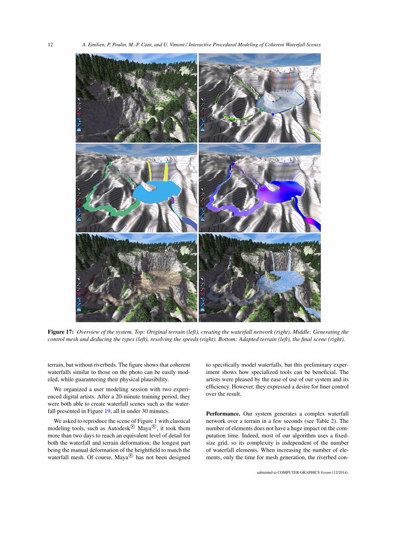
Evaluation. Figures 17 and 18 show an overview of oursystem under editing, with different stages described in thecaption of the figure. An accompanying video gives a muchbetter understanding of our system in action, and illustratesseveral of the features described in the previous sections.

In Figure 1, we show a photo of a real waterfall network,and the result of a 10-minute session with our modeling sys-tem; we started with a terrain resembling the original real



Figure 17: Overview of the system. Top: Original terrain (left), creating the waterfall network (right). Middle: Generating the

control mesh and deducing the types (left), resolving the speeds (right). Bottom: Adapted terrain (left), the final scene (right).

terrain, but without riverbeds. The figure shows that coherentwaterfalls similar to those on the photo can be easily mod-eled, while guaranteeing their physical plausibility.

We organized a user modeling session with two experi-enced digital artists. After a 20-minute training period, theywere both able to create waterfall scenes such as the water-fall presented in Figure 19, all in under 30 minutes.

We asked to reproduce the scene of Figure 1 with classicalmodeling tools, such as Autodesk R© Maya R©, it took themmore than two days to reach an equivalent level of detail forboth the waterfall and terrain deformation; the longest partbeing the manual deformation of the heightfield to match thewaterfall mesh. Of course, Maya R© has not been designed

to specifically model waterfalls, but this preliminary exper-iment shows how specialized tools can be beneficial. Theartists were pleased by the ease of use of our system and itsefficiency. However, they expressed a desire for finer controlover the result.

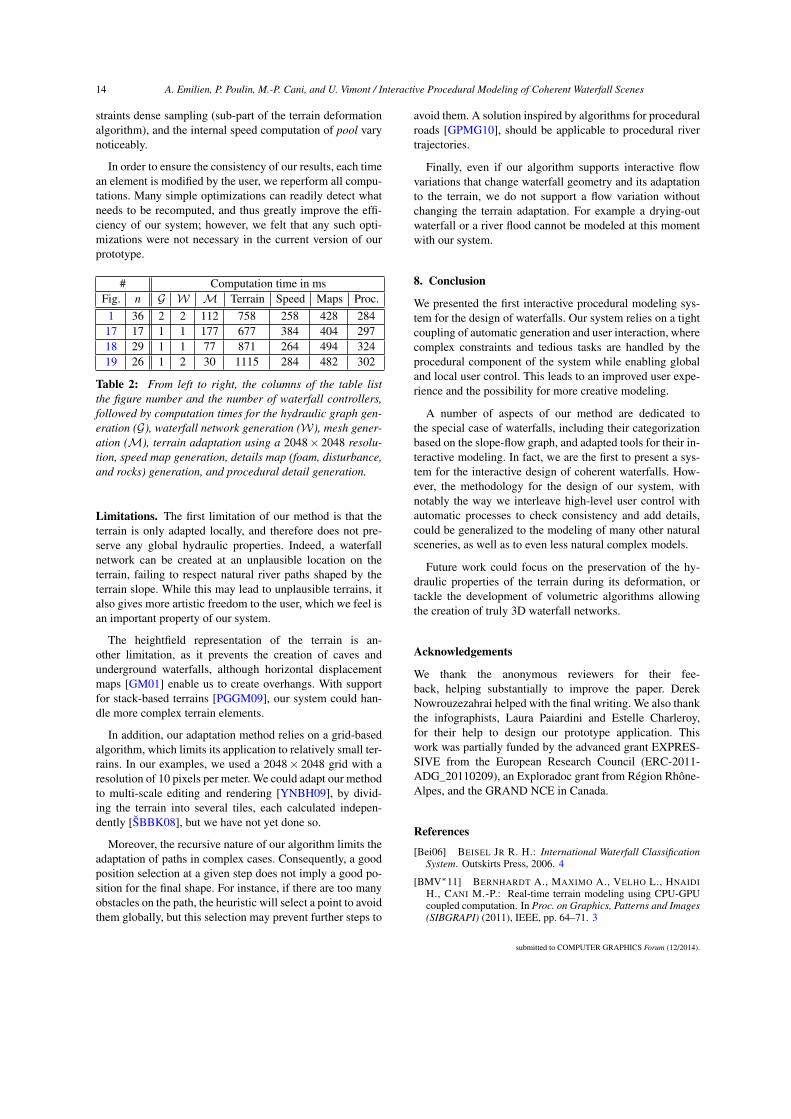
Performance. Our system generates a complex waterfallnetwork over a terrain in a few seconds (see Table 2). Thenumber of elements does not have a huge impact on the com-putation time. Indeed, most of our algorithm uses a fixed-size grid, so its complexity is independent of the numberof waterfall elements. When increasing the number of ele-ments, only the time for mesh generation, the riverbed con-



Figure 18: Another example of waterfall scene. Top left: Controller network. Top right: Integration mesh with types. Bottom

left: Deformed terrain. Bottom right: Final scene.

Figure 19: Waterfalls modeled by one of our digital artists.



straints dense sampling (sub-part of the terrain deformationalgorithm), and the internal speed computation of pool varynoticeably.

In order to ensure the consistency of our results, each timean element is modified by the user, we reperform all compu-tations. Many simple optimizations can readily detect whatneeds to be recomputed, and thus greatly improve the effi-ciency of our system; however, we felt that any such opti-mizations were not necessary in the current version of ourprototype.

# Computation time in msFig. n G W M Terrain Speed Maps Proc.

1 36 2 2 112 758 258 428 28417 17 1 1 177 677 384 404 29718 29 1 1 77 871 264 494 32419 26 1 2 30 1115 284 482 302

Table 2: From left to right, the columns of the table list

the figure number and the number of waterfall controllers,

followed by computation times for the hydraulic graph gen-

eration (G), waterfall network generation (W), mesh gener-

ation (M), terrain adaptation using a 2048× 2048 resolu-

tion, speed map generation, details map (foam, disturbance,

and rocks) generation, and procedural detail generation.

Limitations. The first limitation of our method is that theterrain is only adapted locally, and therefore does not pre-serve any global hydraulic properties. Indeed, a waterfallnetwork can be created at an unplausible location on theterrain, failing to respect natural river paths shaped by theterrain slope. While this may lead to unplausible terrains, italso gives more artistic freedom to the user, which we feel isan important property of our system.

The heightfield representation of the terrain is an-other limitation, as it prevents the creation of caves andunderground waterfalls, although horizontal displacementmaps [GM01] enable us to create overhangs. With supportfor stack-based terrains [PGGM09], our system could han-dle more complex terrain elements.

In addition, our adaptation method relies on a grid-basedalgorithm, which limits its application to relatively small ter-rains. In our examples, we used a 2048× 2048 grid with aresolution of 10 pixels per meter. We could adapt our methodto multi-scale editing and rendering [YNBH09], by divid-ing the terrain into several tiles, each calculated indepen-dently [ŠBBK08], but we have not yet done so.

Moreover, the recursive nature of our algorithm limits theadaptation of paths in complex cases. Consequently, a goodposition selection at a given step does not imply a good po-sition for the final shape. For instance, if there are too manyobstacles on the path, the heuristic will select a point to avoidthem globally, but this selection may prevent further steps to

avoid them. A solution inspired by algorithms for proceduralroads [GPMG10], should be applicable to procedural rivertrajectories.

Finally, even if our algorithm supports interactive flowvariations that change waterfall geometry and its adaptationto the terrain, we do not support a flow variation withoutchanging the terrain adaptation. For example a drying-outwaterfall or a river flood cannot be modeled at this momentwith our system.

8. Conclusion

We presented the first interactive procedural modeling sys-tem for the design of waterfalls. Our system relies on a tightcoupling of automatic generation and user interaction, wherecomplex constraints and tedious tasks are handled by theprocedural component of the system while enabling globaland local user control. This leads to an improved user expe-rience and the possibility for more creative modeling.

A number of aspects of our method are dedicated tothe special case of waterfalls, including their categorizationbased on the slope-flow graph, and adapted tools for their in-teractive modeling. In fact, we are the first to present a sys-tem for the interactive design of coherent waterfalls. How-ever, the methodology for the design of our system, withnotably the way we interleave high-level user control withautomatic processes to check consistency and add details,could be generalized to the modeling of many other naturalsceneries, as well as to even less natural complex models.

Future work could focus on the preservation of the hy-draulic properties of the terrain during its deformation, ortackle the development of volumetric algorithms allowingthe creation of truly 3D waterfall networks.

Acknowledgements

We thank the anonymous reviewers for their fee-back, helping substantially to improve the paper. DerekNowrouzezahrai helped with the final writing. We also thankthe infographists, Laura Paiardini and Estelle Charleroy,for their help to design our prototype application. Thiswork was partially funded by the advanced grant EXPRES-SIVE from the European Research Council (ERC-2011-ADG_20110209), an Exploradoc grant from Région Rhône-Alpes, and the GRAND NCE in Canada.

References

[Bei06] BEISEL JR R. H.: International Waterfall Classification

System. Outskirts Press, 2006. 4

[BMV∗11] BERNHARDT A., MAXIMO A., VELHO L., HNAIDI

H., CANI M.-P.: Real-time terrain modeling using CPU-GPUcoupled computation. In Proc. on Graphics, Patterns and Images

(SIBGRAPI) (2011), IEEE, pp. 64–71. 3



[BN08] BRUNETON E., NEYRET F.: Real-time rendering andediting of vector-based terrains. Computer Graphics Forum (Eu-

rographics) 27, 2 (2008), 311–320. 3, 10

[BSHK04] BHAT K., SEITZ S., HODGINS J., KHOSLA P.: Flow-based video synthesis and editing. ACM Trans. on Graphics

(SIGGRAPH) 23, 3 (2004), 360–363. 2

[BSW10] BAGAR F., SCHERZER D., WIMMER M.: A layeredparticle-based fluid model for real-time rendering of water. Com-

puter Graphics Forum (EGSR) 29, 4 (2010), 1383–1389. 2

[BTHB06] BENEŠ B., TEŠÍNSKY V., HORNYŠ J., BHATIA

S. K.: Hydraulic erosion. Computer Animation and Virtual

Worlds 17, 2 (2006), 99–108. 3

[CEW∗08] CHEN G., ESCH G., WONKA P., MÜLLER P.,ZHANG E.: Interactive procedural street modeling. ACM Trans.

on Graphics 27, 3 (2008), 103. 2

[CM10] CHENTANEZ N., MÜLLER M.: Real-time simulation oflarge bodies of water with small scale details. In Proc. Sympo-

sium on Computer Animation (2010), pp. 197–206. 2

[DD06] DANIELSSON M., DANIELSSON K.: Waterfall Lover’s

Guide Northern California. Mountaineers Books, 2006. 4

[EBP∗12] EMILIEN A., BERNHARDT A., PEYTAVIE A., CANI

M.-P., GALIN E.: Procedural generation of villages on arbitraryterrains. The Visual Computer 28, 6-8 (2012), 809–818. 2

[GCZ∗06] GUAN Y., CHEN W., ZOU L., ZHANG L., PENG Q.:Modeling and rendering of realistic waterfall scenes with dy-namic texture sprites. Computer Animation and Virtual Worlds

17, 5 (2006), 573–583. 2

[GGG∗13] GÉNEVAUX J.-D., GALIN E., GUÉRIN E., PEY-TAVIE A., BENEŠ B.: Terrain generation using procedural mod-els based on hydrology. ACM Trans. on Graphics (SIGGRAPH)

32, 4 (2013), 143:1–13. 2, 3, 9, 10

[GM01] GAMITO M. N., MUSGRAVE F. K.: Procedural land-scapes with overhangs. In 10th Portuguese Computer Graphics

Meeting (2001), vol. 2. 3, 10, 14

[GMS09] GAIN J., MARAIS P., STRASSER W.: Terrain sketch-ing. In Proc. Symposium on Interactive 3D Graphics and Games

(2009), ACM, pp. 31–38. 3

[GPGB11] GALIN E., PEYTAVIE A., GUÉRIN E., BENEŠ B.:Authoring hierarchical road networks. Computer Graphics Fo-

rum (Pacific Graphics) 30, 7 (2011), 2021–2030. 2

[GPMG10] GALIN E., PEYTAVIE A., MARÉCHAL N., GUÉRIN

E.: Procedural generation of roads. Computer Graphics Forum

29, 2 (2010), 429–438. 14

[HGA∗10] HNAIDI H., GUÉRIN E., AKKOUCHE S., PEYTAVIE

A., GALIN E.: Feature based terrain generation using diffusionequation. Computer Graphics Forum (Pacific Graphics) 29, 7(2010), 2179–2186. 3, 9

[HW04] HOLMBERG N., WÜNSCHE B. C.: Efficient modelingand rendering of turbulent water over natural terrain. In Proc.

Intl. Conf. on Computer Graphics and Interactive Techniques in

Australasia and South East Asia (2004), ACM, pp. 15–22. 2, 3

[KM90] KASS M., MILLER G.: Rapid, stable fluid dynamics forcomputer graphics. ACM SIGGRAPH Computer Graphics 24, 4(1990), 49–57. 2

[KW06] KIPFER P., WESTERMANN R.: Realistic and interactivesimulation of rivers. In Proc. Graphics Interface (2006), Cana-dian Information Processing Society, pp. 41–48. 2

[LH04] LOSASSO F., HOPPE H.: Geometry clipmaps: terrain ren-dering using nested regular grids. ACM Trans. on Graphics (SIG-

GRAPH) 23, 3 (2004), 769–776. 3

[LH10] LEE H., HAN S.: Solving the shallow water equationsusing 2D SPH particles for interactive applications. The Visual

Computer 26, 6-8 (2010), 865–872. 2

[LRBP12] LONGAY S., RUNIONS A., BOUDON F.,PRUSINKIEWICZ P.: TreeSketch: Interactive procedural mod-eling of trees on a tablet. In Proc. Symposium on Sketch-Based

Interfaces and Modeling (2012), pp. 107–120. 2

[LWW08] LIPP M., WONKA P., WIMMER M.: Interactive visualediting of grammars for procedural architecture. ACM Trans. on

Graphics 27, 3 (2008), 102:1–10. 2

[MDH07] MEI X., DECAUDIN P., HU B.-G.: Fast hydraulic ero-sion simulation and visualization on gpu. In Proc. Pacific Graph-

ics (2007), IEEE, pp. 47–56. 3

[PGGM09] PEYTAVIE A., GALIN E., GROSJEAN J., MERILLOU

S.: Arches: a framework for modeling complex terrains. Com-

puter Graphics Forum (Eurographics) 28, 2 (2009), 457–467. 3,14

[Plu05] PLUMB G. A.: Waterfall Lover’s Guide Pacific North-

west. Mountaineers Books, 2005. 4

[ŠBBK08] ŠTAVA O., BENEŠ B., BRISBIN M., KRIVÁNEK J.:Interactive terrain modeling using hydraulic erosion. In Proc.

Symposium on Computer Animation (2008), pp. 201–210. 3, 14

[SDKT∗09] SMELIK R., DE KRAKER K., TUTENEL T.,BIDARRA R., GROENEWEGEN S.: A survey of procedural meth-ods for terrain modelling. In Proc. CASA Workshop on 3D Ad-

vanced Media In Gaming And Simulation (3AMIGAS) (2009). 3

[SDZ∗07] SAKAGUCHI R., DUFOR T., ZALZALA J., LAMBERT

P., KAPLER A.: End of the world waterfall setup for “Pirates ofthe Caribbean 3”. In ACM SIGGRAPH Sketches (2007), ACM. 2

[Sta99] STAM J.: Stable fluids. In Proc. SIGGRAPH (1999),pp. 121–128. 11

[STBB14] SMELIK R. M., TUTENEL T., BIDARRA R., BENES

B.: A survey on procedural modelling for virtual worlds. Com-

puter Graphics Forum (2014). 2

[TGM13] TASSE F. P., GAIN J., MARAIS P.: Enhanced texture-based terrain synthesis on graphics hardware. Computer Graph-

ics Forum 31, 6 (2013), 1959–1972. 3

[TMFSG07] THUREY N., MÜLLER-FISCHER M., SCHIRM S.,GROSS M.: Real-time breakingwaves for shallow water simula-tions. In Proc. Pacific Graphics (2007), IEEE, pp. 39–46. 2

[vH11] VAN HOESEL F.: Tiled directional flow. In ACM SIG-

GRAPH Posters (2011), p. 19:1. 3, 11

[YNBH09] YU Q., NEYRET F., BRUNETON E., HOLZSCHUCH

N.: Scalable real-time animation of rivers. Computer Graphics

Forum 28, 2 (2009), 239–248. 2, 3, 14

[YNS11] YU Q., NEYRET F., STEED A.: Feature-based vec-tor simulation of water waves. Computer Animation and Virtual

Worlds 22, 2-3 (2011), 91–98. 3

[ZIH∗11] ZHU B., IWATA M., HARAGUCHI R., ASHIHARA T.,UMETANI N., IGARASHI T., NAKAZAWA K.: Sketch-based dy-namic illustration of fluid systems. ACM Trans. on Graphics

(SIGGRAPH Asia) 30, 6 (2011), 134:1–8. 3, 6, 7

[ZSTR07] ZHOU H., SUN J., TURK G., REHG J. M.: Terrainsynthesis from digital elevation models. IEEE Trans. Visualiza-

tion and Computer Graphics 13, 4 (2007), 834–848. 3


Documents

Interactive Procedural Modelling of Coherent Waterfall … · Interactive Procedural Modelling of Coherent Waterfall Scenes ... Computer Graphics Forum, Wiley, 2015 ... scene contains