Interactions of Energy Storage and Transmission … Final Project...Interactions of Energy Storage and Transmission Expansion Final Report May 2018 Qingyu Xu and Benjamin F. Hobbs

Interactions of Energy Storage and Transmission Expansion

Final Report

May 2018

Qingyu Xu and Benjamin F. Hobbs

Department of Environmental Health & Engineering

Environment, Energy, Sustainability & Health Institute

The Johns Hopkins University

Baltimore, MD

Report Prepared for

The Western Electricity Coordinating Council

WESTERN ELECTRICITY COORDINATING COUNCIL

JHSMINE Storage & Transmission Final Report

i

Disclaimer and Acknowledgments

This material is based upon work supported by the Western Electricity Coordinating Council. All authors performed this work when associated with Johns Hopkins University.

The goal of this project was to demonstrate the potential applicability of a tool to transmission and storage project evaluation, and not to provide an economic evaluation of particular projects. Emphasis has been placed on illustrating model capabilities, and not on quality checking of input assumptions. These assumptions and results have not been reviewed in detail by relevant stake-holders. Therefore, even though particular projects are referred to in this report, any results con-cerning their economic benefits and costs are highly preliminary in nature and should not be re-lied upon for project evaluation and planning. Results should not be cited as supporting any con-clusions concerning the economics of any of the projects.

The project team would like to thank Vijay Satyal, Michael Bailey, Jonathan Jensen, Bharath Ketineni, Byron Woertz, Chris Albrecht, and Andrea Coon of WECC for their support and ad-vice during this project. We would also like to thank our JHU colleagues on the previous WECC-DOE JHSMINE project for their contributions to the development of JHSMINE and its daabases, namely Jonathan Ho (now at NREL), Pearl Donohoo-Vallett (now at Brattle), Saamrat Kasina (now at E-three), Sangwoo Park (now at the University of California, Berkeley), and Jas-mine Ouyang (also at E-Three). However, the authors are solely responsible for any opinions or errors in this document.


ii

Table of Contents

1. INTRODUCTION ...................................................................................................................... 1

2. EXAMPLE LONG-RUN BENEFIT-COST ANALYSES OF LARGE-SCALE AND BATTERY STORAGE: ILLUSTRATION OF JHSMINE CAPABILITIES ................................ 3

2.1 Database update and modeling assumptions ........................................................................ 3

2.1.1 JHSMINE-361 test system for 2034 planning ............................................................... 3

2.1.2. Align JH-361 test system and JHSMINE with WECC-LTPT ...................................... 7

2.1.3 Customable Day Selection Procedure .......................................................................... 16

2.1.4. Generation, Transmission and Storage Expansion Assumptions ............................... 16

2.2 Results of CAES/PHES Analyses ...................................................................................... 18

2.2.1. Impact of CAES/PHES on long-term expansion planning ......................................... 19

2.2.2 Impact of CAES and PHES on the prices .................................................................... 21

2.2.3 Profitability of CAES and PHES ................................................................................. 22

2.2.4 Impact of PHES/CAES on congestion in 2034............................................................ 27

2.3 Comparison of the base and alternative cases to determine the interaction of storage, transmission economics, and renewable integration ................................................................. 30

3. QUALITATIVE ASSESSMENT OF JHSMINE CAPABILITIES TO ADDRESS KEY ISSUES IN PLANNING............................................................................................................... 41

3.1 Public Policy Goals: - Ability of the tool to capture policy goals (state RPS, carve-out, tiers) ...................................................................................................................................... 42

3.2 Resource Adequacy: Framework for assessing resource adequacy to meet annual load energy needs.......................................................................................................................... 43

3.3 Optimal Generation modeling capability: Modeling functionality to assess optimal generation dispatch to minimize cost and alleviate security violations, simulating operational flexibility ............................................................................................................ 44

3.4 Modeling logic and protocol for evaluating transmission expansion when co-optimized with generation portfolios ..................................................................................................... 46

3.5 Reliability considerations including must-run, local and system portfolio and dispatch constraints as a function of load, and flexible portfolio and dispatch constraints as a function of other resource types (e.g., wind & solar) .......................................................................... 47

3.6 Multiple generation, transmission, and substation configurations and corresponding costs....................................................................................................................................... 47


iii

3.7 Geospatial considerations including environmental risk impact, terrain difficulty (e.g., slope, land cover), ROW costs (e.g., BLM zone costs), renewable potentials (e.g., NREL wind and solar) ...................................................................................................................... 48

3.8 Pool constraints (e.g., renewable potential, water availability, carbon constraints) ....... 49

3.9 Seasonal load variations (e.g., load duration blocks) ...................................................... 50

Appendix A. WECC Storage-Transmission Planning Interactions: Selecting Days .................... 51

A.1 Introduction ........................................................................................................................ 51

A.2 Day Selection Procedure .................................................................................................... 51

A.2.1 Importance of proposed method ................................................................................. 52

A.2.2 JHU Day selection procedure: .................................................................................... 52

A.2.3 Day Selection Results ................................................................................................ 55

A.3 Features of the proposed Day Selection procedure ........................................................... 56

A.4 Customization of Day Selection procedure ....................................................................... 56

Appendix B. Generation and Storage Expansion Co-optimization with Consideration of Unit Commitment: Application to Storage-Transmission Relations .................................................... 58


iv

List of Tables

Table 1. Existing Storage Facilities in JH-361 Test System ........................................................... 6 Table 2. LTPT's Load Block Definition ......................................................................................... 7 Table 3. 2026 Common Case Equal Probable Block LDC (JHSMINE Team) (MW) ................... 8 Table 4. 2034 Reference Case Equal Probable Block LDC (MW) ................................................ 9 Table 5. 2026 to 2034 Reshaping Factors obtained by JHSMINE team ...................................... 11 Table 6. Distributed factor from Load Area to State, from CC 2026 ........................................... 13 Table 7. RPS goals in JHSMINE, from LTPT.............................................................................. 14 Table 8. Reliability and Reserve goals in JHSMINE, from LTPT ............................................... 15 Table 9. Day Selection Result ....................................................................................................... 16 Table 10. Base capital cost assumptions in JHSMINE ................................................................. 18 Table 11. Test Cases for Sections 2.2.1, 2.2.2 and 2.2.3, 2.2.4 .................................................... 19 Table 12. Annualized Cost Comparison of Test Cases 1-6 (Annualized Cost, Million $/yr, negative values represent cost reductions) .................................................................................... 20 Table 13. Investment Comparison of Test Cases 1-6 (GW in the Year 2026, online in Year 2034)....................................................................................................................................................... 21 Table 14. 365-day simulation result: LMPs, operating reserve prices and long-term capacity payment rate at IPP in three cases: Case 1: without any of CAES, PHES and Pathfinder wind in system; Case 2: With only PHES in system, and Case 4: with only CAES in system ................. 22 Table 15. Annual (52 weeks) Cost and Benefit of CAES and PSES ($Million/yr), Carbon price $58/Metric ton, transmission and generation fleets expanded as in Case 6 .................................. 24 Table 16. 2034-yearly profit ($M/yr) of CAES in Case 6 (with CAES, PHES and Pathfinder wind installed) in different look-ahead scheme. ........................................................................... 25 Table 17. 2034-yearly profit ($M/yr) of PHES in Case 6 (with CAES, PHES and Pathfinder wind installed) in different look-ahead scheme. .................................................................................... 25 Table 18. CAES Revenue from case with CAES and PHES installed without the construction of Pathfinder wind ............................................................................................................................. 26 Table 19. CAES revenue from case with CAES, PHES and Pathfinder wind installed; carbon price is set to $20/metric ton ......................................................................................................... 26 Table 20. CAES revenue if WECC-wide Hydro is 20% less than base case, but with CAES, PHES and Pathfinder wind installed ............................................................................................. 26 Table 21. Preserved Paths in JH-361 ............................................................................................ 28 Table 22. Test Cases for Task 4 .................................................................................................... 31 Table 23. Cost Comparison of Cases 1-5, Carbon Price $58/Metric ton, 100% BESS cost = $292/kW-yr (Annualized Cost, Billion $/yr) ................................................................................ 32 Table 24. Cost Comparison between Case 6-10, Carbon Price $100/Metric ton, 100% BESS cost = $292/kW-yr (Annualized Cost, Billion $/yr) ............................................................................. 33 Table 25. WREZ Hub and Transmission Investment in Case 1 (No BESS) and 4 (30% of Baseline BESS Cost), Carbon Price: $58/Metric ton, 2034(GW) ................................................ 39 Table 26. WREZ Hub and Transmission Investment in Case 6 (No BESS) and 9 (30% of Baseline level BESS Cost), Carbon Price: $100/Metric ton, 2034(GW) ..................................... 40 Table 27. Profiles Included in Day Selection ............................................................................... 51


v

Table 28. Bin Assignment Definition ........................................................................................... 52 Table 29. Nomenclature for Similarity Score Calculation ............................................................ 53 Table 30. Clustering Result with K=4 .......................................................................................... 54 Table 31. Pros and Cons of Random Selection plus Result Filtering Approach .......................... 55 Table 32. Day Selection Optimization .......................................................................................... 55 Table 33. Pros and Cons of Integer Programming Approach ....................................................... 55 Table 34. Day Selection Result of Approach 2 ............................................................................. 56 Table 35. The First Moment Deviation of the Year Comprised of Selected Days against the Original year ................................................................................................................................. 56 Table 36. Customization of Proposed Day Selection ................................................................... 57


vi

List of Figures

Figure 1. JH-361 Test Network ...................................................................................................... 5 Figure 2. Winter Heavy Loads for 2026 (Common Case, x-axis) and 2034 (Reference Case, y-axis). .............................................................................................................................................. 10 Figure 3. 2026 and 2034 Load Profiles for Alberta (AESO) (in MWs) ....................................... 12 Figure 4. Analysis Road Map for Analysis of Section 2.2 ........................................................... 18 Figure 5. Charge and discharge duration curve of CAES/PSES (Positive: Generation) .............. 23 Figure 6. Path Utilization (U75) in 2034, a comparison between Case 1 (without CAES/PHES/Pathfinder) and Case 6 (with CAES/PHES/Pathfinder); Paths with U75 lower than 15% in both Case 1 and 6 NOT shown ......................................................................................... 29 Figure 7. Path Utilization (U90) in 2034, a comparison between Case 1 (without CAES/PHES/Pathfinder) and Case 6 (with CAES/PHES/Pathfinder); Paths with U90 lower than 10% in both Case 1 and 6 NOT shown ......................................................................................... 29 Figure 8. Path Utilization (U99) in 2034, a comparison between Case 1 (without CAES/PHES/Pathfinder) and Case 6 (with CAES/PHES/Pathfinder); Paths with U99 lower than 5% in both Case 1 and 6 NOT shown ........................................................................................... 30 Figure 9. Analysis Road Map for Section 2.3 ............................................................................... 30 Figure 10. WECC-wide generation production mix for Cases 1, 4, 6 and 9. (2034 TWh) .......... 34 Figure 11. Cases 1-5: Generation capacity and storage additions in 2034 (GW, left axis), and carbon intensity (metric T/GWh, red dashes, right axis), carbon price = $58/Metric ton ............ 35 Figure 12. Cases 6-10: Generation and storage expansion (left axis) and carbon intensity (red dashes, right axis), carbon price = $100/Metric ton...................................................................... 36 Figure 13. Backbone Reinforcements in Case 1-5 (left) and Case 6-10 (right). Red-circled line is cancelled when BESS cost is 20% of baseline level ..................................................................... 37 Figure 14. Map of WREZ Hubs .................................................................................................... 38 Figure 15. Bin Assignment for Wind Profile of Alberta January (Daily, colors other than red), and yearly average (red). X axis are bins and Y axis are number of hours in the bins ................. 53


1

1. INTRODUCTION

This document serves as the final product of the project Interactions of Energy Storage and Transmission Expansion, as described in the “WECC-Johns Hopkins University Services Con-tact, Exhibit A-Statement of Work”, as modified on Nov. 13, 2017.

This project is a follow-on to an earlier WECC-sponsored project in which the Johns Hopkins Stochastic Multistate Integrated Network Expansion model (JHMSINE) was used to analyze the value of uncertainty-based planning for the Western Electricity Coordinating Council region.1

There are two phases in this project, whose results are reported in separate sections of this report. The goal of the first phase, which is reported in Section 2, is to conduct an initial analysis of in-teractions of electricity transmission and storage economics for two realistic large-scale storage projects using the 2026 CCTA data base. Questions addressed are whether storage and transmis-sion are substitutes (building one lowers the value of the other) or complements (building one increases the value of the other), and how storage affects the value of renewables and transmis-sion in different locations. This analysis is highly preliminary in nature, in that it is based on un-reviewed data input assumptions, and is intended to illustrate the functionality of the JHSMINE model used to conduct the analysis.

In this first phase, the two projects considered are:

an Oregon/Washington State pumped storage facility located near the northern end of the Pacific Coast AC and DC interties; and

a 1200 MW Compressed Air Energy Storage facility located near the Intermountain Power Plant (Delta, UT).

The impact of those projects on the economics of new transmission and generation resources in the WECC region are be assessed by comparing the results of JHSMINE runs with and without those projects. The results that will be compared include the location and timing of recom-mended investments in WECC in new facilities, fuel mixes, congestion and production costs, and CO2 emissions. If the model shows that implementation of the storage projects increases the profitability or likelihood of construction of some transmission, then a complementarity is identi-fied. On the other hand, decreased profitability or likelihood of construction indicates that stor-

1 J.L. Ho, B.F. Hobbs, P. Donohoo-Vallett, Q. Xu, S. Kasina, S.W. Park, and Y. Ouyang, Planning Transmission for Uncertainty: Applications and Lessons for the Western Interconnection, Final Report, Johns Hopkins University, Prepared for the Western Electricity Coordinating Council, Jan. 2016, www.wecc.biz/Reliability/Planning-for-Uncertainty-Final-Report.pdf. This work was summarized in B.F. Hobbs, Q. Xu, J. Ho, P. Donohoo, S. Kasina, J. Ouyang, S.W. Park, J. Eto, and V. Satyal, Adaptive Transmission Planning: Implementing a New Paradigm for Managing Economic Risks in Grid Expansion, IEEE Power & Energy Magazine, 14(4), July-August 2016, 30-40.


2

age and transmission have a substitution type of relationship. We also examine how those facili-ties affect the optimal locations of new renewable investment, in the form of battery storage sys-tems.

In the second phase of the study, an assessment is conducted of the present and potential capabil-ities of JHSMINE to perform transmission-generation-storage co-optimization analyses, and to capture aspects of the technical and economic systems that determine the net benefits of trans-mission. Section 3 presents the results of this phase of the project.

Two Appendices are also provided in this report. In Appendix A, we describe the day selection method used to choose the days to include in the JHSMINE investment planning model, since it is not possible to include 365 days per year in the planning model. In Appendix B, a published paper that explores the complementary and substitution relations of renewable resources and bat-tery storage is reproduced;2 this paper is based on some of the methods and data developed in Section 2.

2Qingyu Xu, Shenshen Li, and Benjamin F. Hobbs, “Generation and Storage Expansion Co-optimization with Consideration of Unit Commitment”, to Appear, Proceedings of the Probabilistic Methods Applied to Power Systems Conference, Probabilistic Methods: Practical Approaches for Managing Risk and Uncertainty in the Electric Power Industry, Boise Idaho, June 24, 28, 2018


3

2. EXAMPLE LONG-RUN BENEFIT-COST ANALYSES OF LARGE-SCALE AND BATTERY STORAGE: ILLUSTRATION OF JHSMINE

CAPABILITIES

In this section of the report, we summarize the JHSMINE database update, and modeling as-sumptions on the storage studies using the JHSMINE tool. Results of the analyses of CAES/PHES modeled technologies and resulting impacts are then reported in the subsequent subsections on the following results: costs, congestion levels, potential need for new transmis-sion or not, production costs and related CO2 emissions.

This section of the report is composed of three parts. In Section 2.1, we document the database updates and general modeling assumptions for all the analyses in Sections 2.2 and 2.3 of this re-port. In Section 2.2, the capability of the JHSMINE tool to perform analyses of impact of Com-pressed Air Energy Storage (CAES) and Pumped Hydro Energy Storage (PHES) on long-term planning is illustrated. Then in Section 2.3, we explore the sources and amounts of revenue from capacity markets and spot markets, including energy and operating reserves. In Section 2.4, the analysis of the interaction of storage, transmission economics, and renewable integration is docu-mented, with a focus on battery energy storage systems.

These results are intended to illustrate the capabilities of the model and should not be interpreted as a planning or project financial analysis. Limitations include simplifications of the production costing model (e.g., limited number of operating hours considered in the planning model) and a simplified set of demand and generation cost assumptions that have not been subjected to stake-holder review.

2.1 Database update and modeling assumptions

In this section, the JHSMINE team documents all the data preparation for storage analyses of the Phase 1 analysis. This includes building the JH-361 test system, enabling JHSMINE to storage operation (Section 2.1.1), assumption harmonization between JHSMINE+JH361 system with LTPT (Section 2.1.2) and finally a highly customable procedure for selecting hours/days for the planning model (Section 2.1.3).

2.1.1 JHSMINE-361 test system for 2034 planning

o Summary: A reduced network (here after as JH-361 System) is constructed for the 2034 plan-ning period.

o Transmission Network Description: A network reduction algorithm3 has been applied to the network provided in 2026 Common Case Version 1.5. A new set of preserved buses has been selected by combining the experience of the previous JHU reduction (referred to as the “300-

3 Discussed in J.L. Ho et al., Footnote 1, supra. The methodology is based on Y. Zhu & D. Tylavsky, “An optimization-based dc-network reduction method,” IEEE Transactions on Power Systems, 33(3), 2509-2517, 2018.


4

bus network”) and the new network topology in the 2026 Common Case. Some post-reduc-tion adjustments have been made.

The new network has 361 preserved buses, 414 preserved high-voltage (230 kV and above) AC lines, 5 preserved DC lines, 473 equivalent lines, and 15 modified AC lines. Equivalent lines are the calculated results of a reduction algorithm applied to non-preserved AC lines. Modified lines are AC lines modified to eliminate negative impedances in the test system, which are usually a result of serial capacitor compensation. A map showing preserved lines and buses are shown in Figure 1 (left), below.

o Generator Description: Generators are aggregated from the latest 2026 Common Case Ver-sion 2.0. There are up to 848 aggregated generators in the system. The total number of gener-ators depends on whether the user assumes that generators under-review, planned, or concep-tual will be online. There are 53 WREZ hubs where renewables can be constructed, as in the previous 300-bus system. Generator capacity is derated to account for expected forced out-ages.


5

Figure 1. JH-361 Test Network

6

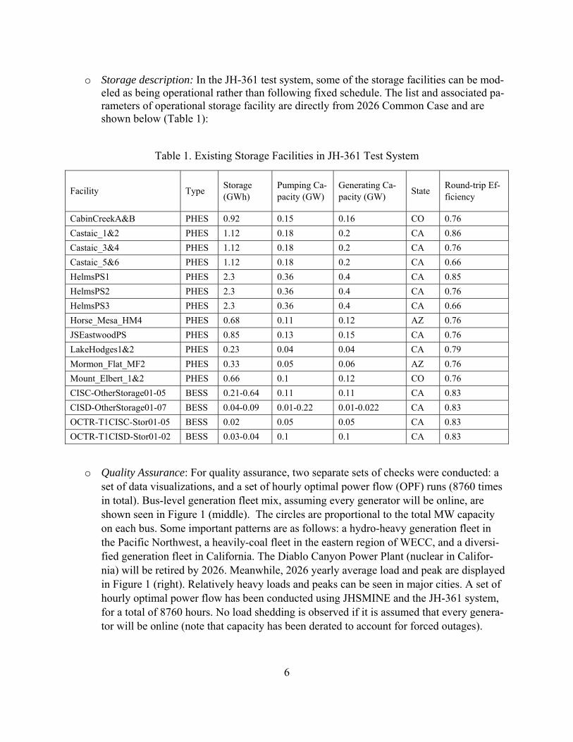
o Storage description: In the JH-361 test system, some of the storage facilities can be mod-eled as being operational rather than following fixed schedule. The list and associated pa-rameters of operational storage facility are directly from 2026 Common Case and are shown below (Table 1):

Table 1. Existing Storage Facilities in JH-361 Test System

Facility Type Storage (GWh)

Pumping Ca-pacity (GW)

Generating Ca-pacity (GW)

State Round-trip Ef-ficiency

CabinCreekA&B PHES 0.92 0.15 0.16 CO 0.76

Castaic_1&2 PHES 1.12 0.18 0.2 CA 0.86

Castaic_3&4 PHES 1.12 0.18 0.2 CA 0.76

Castaic_5&6 PHES 1.12 0.18 0.2 CA 0.66

HelmsPS1 PHES 2.3 0.36 0.4 CA 0.85

HelmsPS2 PHES 2.3 0.36 0.4 CA 0.76

HelmsPS3 PHES 2.3 0.36 0.4 CA 0.66

Horse_Mesa_HM4 PHES 0.68 0.11 0.12 AZ 0.76

JSEastwoodPS PHES 0.85 0.13 0.15 CA 0.76

LakeHodges1&2 PHES 0.23 0.04 0.04 CA 0.79

Mormon_Flat_MF2 PHES 0.33 0.05 0.06 AZ 0.76

Mount_Elbert_1&2 PHES 0.66 0.1 0.12 CO 0.76

CISC-OtherStorage01-05 BESS 0.21-0.64 0.11 0.11 CA 0.83

CISD-OtherStorage01-07 BESS 0.04-0.09 0.01-0.22 0.01-0.022 CA 0.83

OCTR-T1CISC-Stor01-05 BESS 0.02 0.05 0.05 CA 0.83

OCTR-T1CISD-Stor01-02 BESS 0.03-0.04 0.1 0.1 CA 0.83

o Quality Assurance: For quality assurance, two separate sets of checks were conducted: a set of data visualizations, and a set of hourly optimal power flow (OPF) runs (8760 times in total). Bus-level generation fleet mix, assuming every generator will be online, are shown seen in Figure 1 (middle). The circles are proportional to the total MW capacity on each bus. Some important patterns are as follows: a hydro-heavy generation fleet in the Pacific Northwest, a heavily-coal fleet in the eastern region of WECC, and a diversi-fied generation fleet in California. The Diablo Canyon Power Plant (nuclear in Califor-nia) will be retired by 2026. Meanwhile, 2026 yearly average load and peak are displayed in Figure 1 (right). Relatively heavy loads and peaks can be seen in major cities. A set of hourly optimal power flow has been conducted using JHSMINE and the JH-361 system, for a total of 8760 hours. No load shedding is observed if it is assumed that every genera-tor will be online (note that capacity has been derated to account for forced outages).

7

2.1.2. Align JH-361 test system and JHSMINE with WECC-LTPT

o Summary: The structure of JHSMINE and assumptions of the JH-361 network have been updated to align with LTPT to the maximum extent. These changes include reshaped load profiles, reliability and reserve goals, renewable portfolio goals, and pool constraints (maximum allowable installable capacity at a given location).

o Load profile alignment: Since it has been confirmed that hourly profiles for 2034 load were not available and will not be, JHSMINE team utilized LTPT’s equal-probable 8 block definition and 2026 common case profile. A definition of LTPT load blocks can be found below:

Table 2. LTPT's Load Block Definition

Season-Heavy/Lite Begin Date End Date Winter-Heavy 01/01/2034 03/31/2034 Winter-Lite 01/01/2034 03/31/2034 Spring-Heavy 04/01/2034 06/30/2034 Spring-Lite 04/01/2034 06/30/2034 Summer-Heavy 07/01/2034 09/30/2034 Summer-Lite 07/01/2034 09/30/2034 Autumn-Heavy 10/01/2034 12/31/2034 Autumn-Lite 10/01/2034 12/31/2034

The JHSMINE team reshaped the 2026 Common Case area load profiles into 2034 area load pro-files, which satisfied the requirement that if newly reshaped profiles were divided into 8 load blocks for each area, they will correspond to the LTPT 2034 load blocks. The procedure can be found below. This approach can be utilized to obtain any 2034 load hourly profile if we are given LTPT’s load blocks; this capability might be used if other scenarios are constructed by the LTPT team.

1) For each area-level 2026 load profile, JHSMINE team divided it into 4 seasons, according to the following table.

2) For each area-level seasonal load profile, JHSMINE team calculate the median; all load above median will be defined as “heavy”, otherwise “lite”.

3) For each area-level seasonal load profile, calculate the average among “heavy” and “lite”. Basically, Steps 2 and 3 construct the seasonal load duration curve (LDC) for 2026 area-level load assuming equal durations. The results can be found below:

8

Table 3. 2026 Common Case Equal Probable Block LDC (JHSMINE Team) (MW)

2024 Season

Winter Spring Summer Autumn Winter Spring Summer Autumn

H/L Heavy Heavy Heavy Heavy Lite Lite Lite Lite AESO 13164 11709 12130 13012 11765 10396 10618 11353 AVA 1899 1591 1701 1863 1531 1234 1273 1432 AZPS 4205 5531 7173 4410 3552 3633 4695 3583 BANC 2319 2644 3178 2297 1402 1423 1599 1488 BCHA 10201 8579 8455 10134 8373 6780 6632 7830 BPAT 8288 7121 7253 8224 6553 5635 5759 6254 CFE 1597 2063 2568 1729 1262 1497 1932 1335 CHPD 599 466 472 578 507 405 417 472 CIPB 5766 5728 6062 5871 4064 3966 4121 4070 CIPV 7763 9207 10669 7820 5370 6532 7250 5409 CISC 12427 13388 16423 12752 9827 10249 11780 9827 CISD 2810 2831 3393 2941 2086 2048 2320 2099 DOPD 318 218 242 313 227 153 172 209 EPE 1101 1376 1589 1132 797 825 1060 800 GCPD 673 713 801 708 575 600 659 596 IID 461 752 976 531 310 398 520 324 IPFE 325 361 412 324 278 255 283 261 IPMV 579 808 921 590 499 511 664 467 IPTV 1395 1419 1857 1438 1157 1079 1268 1111 LDWP 3831 3936 4679 3884 2405 2484 2670 2493 NEVP 3282 4476 5199 3191 3092 3066 3768 2608 NWMT 1601 1409 1585 1558 1379 1206 1253 1314 PACW 2911 2567 2798 2868 2270 1964 2037 2144 PAID 802 792 890 772 646 603 651 577 PAUT 4401 4309 5307 4391 3713 3416 3837 3671 PAWY 1413 1383 1436 1408 1257 1208 1183 1247 PGE 3236 2914 3062 3206 2545 2254 2258 2419 PNM 1795 1802 2208 1771 1486 1373 1581 1453 PSCO 5585 5475 6412 5518 4552 4221 4463 4483 PSEI 4320 3440 3409 4355 3527 2867 2676 3230 SCL 1486 1255 1229 1472 1172 974 951 1103 SPPC 1244 1635 1895 1207 1062 1095 1352 893 SRP 3824 4916 6494 3969 3079 3055 4191 3032 TEPC 1917 2458 2914 1983 1628 1689 2079 1661 TIDC 341 421 534 371 269 303 346 281 TPWR 836 647 617 803 664 518 494 606 VEA 74 78 102 86 52 48 66 56 WACM 4020 3915 4615 4160 3536 3516 3657 3629 WALC 1391 1682 1476 1187 998 1314 1001 961 WAUW 127 112 129 125 103 83 95 85

4) The counterpart LDC in 2034 has been provided by LTPT team, and is shown in the fol-lowing table:

9

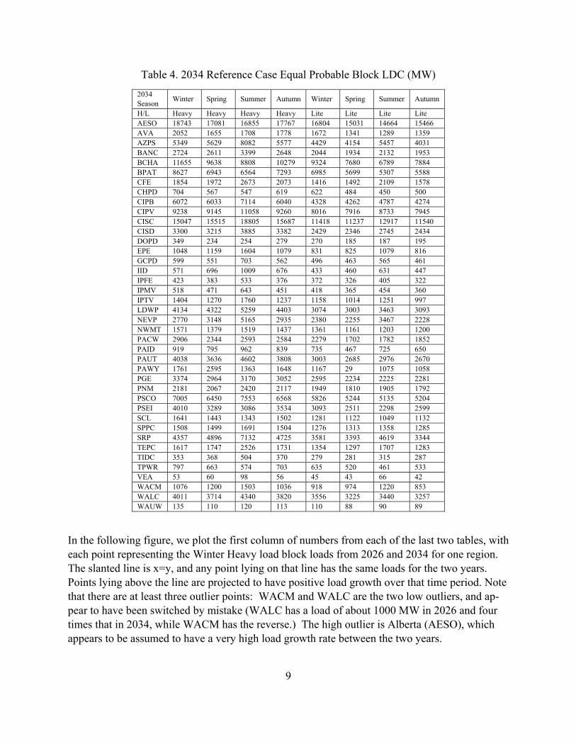
Table 4. 2034 Reference Case Equal Probable Block LDC (MW)

2034 Season

Winter Spring Summer Autumn Winter Spring Summer Autumn

H/L Heavy Heavy Heavy Heavy Lite Lite Lite Lite AESO 18743 17081 16855 17767 16804 15031 14664 15466 AVA 2052 1655 1708 1778 1672 1341 1289 1359 AZPS 5349 5629 8082 5577 4429 4154 5457 4031 BANC 2724 2611 3399 2648 2044 1934 2132 1953 BCHA 11655 9638 8808 10279 9324 7680 6789 7884 BPAT 8627 6943 6564 7293 6985 5699 5307 5588 CFE 1854 1972 2673 2073 1416 1492 2109 1578 CHPD 704 567 547 619 622 484 450 500 CIPB 6072 6033 7114 6040 4328 4262 4787 4274 CIPV 9238 9145 11058 9260 8016 7916 8733 7945 CISC 15047 15515 18805 15687 11418 11237 12917 11540 CISD 3300 3215 3885 3382 2429 2346 2745 2434 DOPD 349 234 254 279 270 185 187 195 EPE 1048 1159 1604 1079 831 825 1079 816 GCPD 599 551 703 562 496 463 565 461 IID 571 696 1009 676 433 460 631 447 IPFE 423 383 533 376 372 326 405 322 IPMV 518 471 643 451 418 365 454 360 IPTV 1404 1270 1760 1237 1158 1014 1251 997 LDWP 4134 4322 5259 4403 3074 3003 3463 3093 NEVP 2770 3148 5165 2935 2380 2255 3467 2228 NWMT 1571 1379 1519 1437 1361 1161 1203 1200 PACW 2906 2344 2593 2584 2279 1702 1782 1852 PAID 919 795 962 839 735 467 725 650 PAUT 4038 3636 4602 3808 3003 2685 2976 2670 PAWY 1761 2595 1363 1648 1167 29 1075 1058 PGE 3374 2964 3170 3052 2595 2234 2225 2281 PNM 2181 2067 2420 2117 1949 1810 1905 1792 PSCO 7005 6450 7553 6568 5826 5244 5135 5204 PSEI 4010 3289 3086 3534 3093 2511 2298 2599 SCL 1641 1443 1343 1502 1281 1122 1049 1132 SPPC 1508 1499 1691 1504 1276 1313 1358 1285 SRP 4357 4896 7132 4725 3581 3393 4619 3344 TEPC 1617 1747 2526 1731 1354 1297 1707 1283 TIDC 353 368 504 370 279 281 315 287 TPWR 797 663 574 703 635 520 461 533 VEA 53 60 98 56 45 43 66 42 WACM 1076 1200 1503 1036 918 974 1220 853 WALC 4011 3714 4340 3820 3556 3225 3440 3257 WAUW 135 110 120 113 110 88 90 89

In the following figure, we plot the first column of numbers from each of the last two tables, with each point representing the Winter Heavy load block loads from 2026 and 2034 for one region. The slanted line is x=y, and any point lying on that line has the same loads for the two years. Points lying above the line are projected to have positive load growth over that time period. Note that there are at least three outlier points: WACM and WALC are the two low outliers, and ap-pear to have been switched by mistake (WALC has a load of about 1000 MW in 2026 and four times that in 2034, while WACM has the reverse.) The high outlier is Alberta (AESO), which appears to be assumed to have a very high load growth rate between the two years.

10

Figure 2. Winter Heavy Loads for 2026 (Common Case, x-axis) and 2034 (Reference Case, y-axis).

5) Thus, the load reshaping factors can be obtained by dividing the 2034 LDC block values by the 2026 LDC values for each region and period. Then for each hour within a given block and region, that factor can be multiplied by the Common Case 2026 load for that hour to obtain the assumed 2034 load. The next table shows these load reshaping factors.

0

2000

4000

6000

8000

10000

12000

14000

16000

18000

20000

0 2000 4000 6000 8000 10000 12000 14000

2034

Win

ter

Hea

vy L

oad

(MW

)

2026 Winter Heavy Load (MW)

11

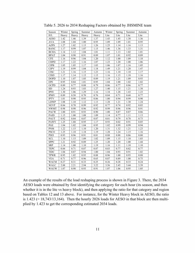
Table 5. 2026 to 2034 Reshaping Factors obtained by JHSMINE team

Season Winter Spring Summer Autumn Winter Spring Summer Autumn H/L Heavy Heavy Heavy Heavy Lite Lite Lite Lite AESO 1.42 1.46 1.39 1.37 1.43 1.45 1.38 1.36 AVA 1.08 1.04 1.00 0.95 1.09 1.09 1.01 0.95 AZPS 1.27 1.02 1.13 1.26 1.25 1.14 1.16 1.13 BANC 1.17 0.99 1.07 1.15 1.46 1.36 1.33 1.31 BCHA 1.14 1.12 1.04 1.01 1.11 1.13 1.02 1.01 BPAT 1.04 0.98 0.91 0.89 1.07 1.01 0.92 0.89 CFE 1.16 0.96 1.04 1.20 1.12 1.00 1.09 1.18 CHPD 1.17 1.22 1.16 1.07 1.23 1.20 1.08 1.06 CIPB 1.05 1.05 1.17 1.03 1.06 1.07 1.16 1.05 CIPV 1.19 0.99 1.04 1.18 1.49 1.21 1.20 1.47 CISC 1.21 1.16 1.15 1.23 1.16 1.10 1.10 1.17 CISD 1.17 1.14 1.15 1.15 1.16 1.15 1.18 1.16 DOPD 1.10 1.07 1.05 0.89 1.19 1.21 1.09 0.93 EPE 0.95 0.84 1.01 0.95 1.04 1.00 1.02 1.02 GCPD 0.89 0.77 0.88 0.79 0.86 0.77 0.86 0.77 IID 1.24 0.93 1.03 1.27 1.40 1.15 1.21 1.38 IPFE 1.30 1.06 1.29 1.16 1.34 1.28 1.43 1.23 IPMV 0.89 0.58 0.70 0.76 0.84 0.71 0.68 0.77 IPTV 1.01 0.90 0.95 0.86 1.00 0.94 0.99 0.90 LDWP 1.08 1.10 1.12 1.13 1.28 1.21 1.30 1.24 NEVP 0.84 0.70 0.99 0.92 0.77 0.74 0.92 0.85 NWMT 0.98 0.98 0.96 0.92 0.99 0.96 0.96 0.91 PACW 1.00 0.91 0.93 0.90 1.00 0.87 0.87 0.86 PAID 1.15 1.00 1.08 1.09 1.14 0.77 1.11 1.13 PAUT 0.92 0.84 0.87 0.87 0.81 0.79 0.78 0.73 PAWY 1.25 1.88 0.95 1.17 0.93 0.02 0.91 0.85 PGE 1.04 1.02 1.04 0.95 1.02 0.99 0.99 0.94 PNM 1.22 1.15 1.10 1.20 1.31 1.32 1.21 1.23 PSCO 1.25 1.18 1.18 1.19 1.28 1.24 1.15 1.16 PSEI 0.93 0.96 0.91 0.81 0.88 0.88 0.86 0.80 SCL 1.10 1.15 1.09 1.02 1.09 1.15 1.10 1.03 SPPC 1.21 0.92 0.89 1.25 1.20 1.20 1.00 1.44 SRP 1.14 1.00 1.10 1.19 1.16 1.11 1.10 1.10 TEPC 0.84 0.71 0.87 0.87 0.83 0.77 0.82 0.77 TIDC 1.04 0.87 0.94 1.00 1.04 0.93 0.91 1.02 TPWR 0.95 1.02 0.93 0.88 0.96 1.00 0.93 0.88 VEA 0.71 0.77 0.96 0.65 0.87 0.89 1.00 0.75 WACM 0.27 0.31 0.33 0.25 0.26 0.28 0.33 0.24 WALC 2.88 2.21 2.94 3.22 3.56 2.45 3.44 3.39 WAUW 1.07 0.98 0.93 0.91 1.07 1.06 0.95 1.05

An example of the results of the load reshaping process is shown in Figure 3. There, the 2034 AESO loads were obtained by first identifying the category for each hour (its season, and then whether it is in the lite vs heavy block), and then applying the ratio for that category and region based on Tables 12 and 13 above. For instance, for the Winter Heavy block in AESO, the ratio is 1.423 (= 18,743/13,164). Then the hourly 2026 loads for AESO in that block are then multi-plied by 1.423 to get the corresponding estimated 2034 loads.

12

Figure 3. 2026 and 2034 Load Profiles for Alberta (AESO) (in MWs)

o Generation expansion-RPS goals alignment: The renewable portfolio standards (RPS) constraints are modified to align with LTPT. It is should be mentioned that: 1) if a RPS goal is specified by the type of utility, this goal will be guaranteed to be satisfied since the more generic RPS goal (state-level) has to be satisfied; 2) earmarked renewable re-source goals are approximated by making the assumption that every renewable generator will meet the RPS of the state where it is geographically located or of the state that was specified by common case; 3) the REC trading system in JHSMINE has been turned off, thus no-instate renewable requirement is needed;4 4) since distributed generation is not an investment option in JHSMINE, RPS goals for DG are not modeled; and 5) to align with LTPT tools, hydropower is credited towards RPS goals in all jurisdictions except for Cal-ifornia. For each state, in order to calculate renewable energy requirements, it is necessary to esti-mate state-level total energy. This is done by redistributing the total energy load at the

4 Note that the absence or presence of REC trading among states can have a significant effect on generation mixes and transmission plans. See A.P. Perez, E.E. Sauma, F.D. Munoz, and B.F. Hobbs, “The Economic Effects of Interregional Trading of Renewable Energy Certificates in the WECC,” The Energy Journal, 37(4), 2016, 267-296.

7500

9500

11500

13500

15500

17500

19500

21500

121

041

962

883

710

4612

5514

6416

7318

8220

9123

0025

0927

1829

2731

3633

4535

5437

6339

7241

8143

9045

9948

0850

1752

2654

3556

4458

5360

6262

7164

8066

8968

9871

0773

1675

2577

3479

4381

5283

6185

70

AESO-2034 AESO-2026

13

BA-level load to the state; the required distribution factors are derived from the 2026 common case and can be found below:

Table 6. Distributed factor from Load Area to State, from CC 2026

Load Area State Ratio Load Area State Ratio AESO AB 100.00% PNM NM 100.00% AZPS AZ 100.00% EPE NM 21.59% SRP AZ 100.00% WACM NM 5.05% TEPC AZ 100.00% WALC NM 6.03% WALC AZ 72.70% PGE OR 100.00% BCHA BC 100.00% PACW OR 73.90% CIPB CA 100.00% BPAT OR 24.70% CIPV CA 100.00% EPE TX 78.41% CISC CA 100.00% PAUT UT 100.00% CISD CA 100.00% WACM UT 3.50% IID CA 100.00% WALC UT 0.57% LDWP CA 100.00% BPAT UT 0.07% BANC CA 100.00% NEVP UT 0.13% TIDC CA 100.00% BPAT WA 68.56% PACW CA 4.52% AVA WA 65.04% WALC CA 18.55% PACW WA 21.57% PSCO CO 100.00% PSEI WA 100.00% WACM CO 64.20% SCL WA 100.00% AVA ID 34.96% TPWR WA 100.00% PAID ID 100.00% CHPD WA 100.00% BPAT ID 2.74% DOPD WA 100.00% NWMT MT 100.00% GCPD WA 100.00% WAUW MT 100.00% PAWY WY 100.00% BPAT MT 3.62% WACM WY 27.25% AVA MT 0.01% CFE MX 100.00% NEVP NV 99.87% IPFE ID 95.61% SPPC NV 100.00% IPFE OR 4.39% BPAT NV 0.31% IPMV ID 95.61% WALC NV 2.16% IPMV OR 4.39% VEA NV 100.00% IPTV ID 95.61% PACW NV 0.00% IPTV OR 4.39%

For each state, the RPS goal is obtained directly from latest LTPT data and is shown below. These goals have to be satisfied in JHSMINE, or a penalty of 100 $/MWh will apply.

14

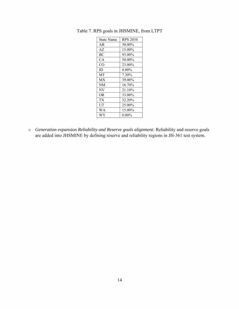
Table 7. RPS goals in JHSMINE, from LTPT

State Name RPS 2034 AB 30.00% AZ 15.00% BC 93.00% CA 50.00% CO 23.00% ID 0.00% MT 7.30% MX 39.00% NM 16.70% NV 21.10% OR 33.00% TX 32.20% UT 25.00% WA 15.00% WY 0.00%

o Generation expansion Reliability and Reserve goals alignment: Reliability and reserve goals are added into JHSMINE by defining reserve and reliability regions in JH-361 test system.

15

Table 8. Reliability and Reserve goals in JHSMINE, from LTPT

Reliability Area

Reliability Goals Reserve Goals

Eligibility (generators in the specified state)

Margin

Eligibility (generators in the specified reserve re-gions)

Margin

AB AB 1% Alberta 3% AZ AZ 0.5% AZ-NM-NV 0.75% BC BC 1% British Columbia 3% CA-NO (44.44% of CA)

CA 0.5% CA-North 0.75%

CA-SO (55.56% of CA)

CA 1% CA-South 2.7%

CO CO 1% RMPA 2.7% ID ID 0.5% Basin 0.75% MT MT 0.5% NWPP 0.75% MX MX 1% Mexico 3% NM NM 1% AZ-NM-NV 2.7% NV-NO (31.55% of NV)

NV 0.5% Basin 0.75%

NV-SO (68.45% of NV)

NV 1% AZ-NM-NV 2.7%

OR OR 0.5% NWPP 0.75% TX TX 1% AZ-NM-NV 2.7% UT UT 0.5% Basin 0.75% WA WA 0.5% NWPP 0.75% WY WY 0.5% RMPA 2.7%

All reliability and reserve goals are modeled using the following constraints:

∗

1 ∗

The effective load carrying capability (ELCC) for each resource type is directly from the LTPT.

o Pool constraints and generation candidates: for renewable generation candidates, JHSMINE has been aligned with the assumption in LTPT that renewables are located on the WREZ hub and are limited by the pool constraints for each fuel type: wind, solar, geothermal and bio-mass. To limit the number of decision variables, wind is assumed to be onshore wind, while solar is assumed to be utility-scale photovoltaic. Overnight capital costs of generation, trans-

16

mission and storage facilities are based on the latest TEPPC Generation Capital Cost Calcu-lator5 and TEPPC Transmission Capital Cost Calculator.6 More details are described below under Section 2.1.4, below.

o Changes from Common Case 2026: For hydroelectric facilities in British Columbia that are scheduled to retired between 2027-2033, the retirement dates are postponed, making sure that BC has enough hydro in 2034.

2.1.3 Customable Day Selection Procedure

o Summary: A highly customizable day selection procedure based on a clustering methodology has been developed to develop the data base that meets the chronological data requirements of storage modeling. Four days (96 hours) are selected by this procedure and they form one key input of the model runs for other results in this report. The procedure is documented in the appendix.

o The selected four days and their associated cluster are summarized in the following table.

Table 9. Day Selection Result Day Cluster (Day 1 as Jan. 1st) 1-124, 290-365 125-174 175-251 252-289 Representative Day 31 (Jan. 31st) 159 (June 8th) 200 (July 19th) 275 (Oct. 2nd) Cluster Size 200 50 77 38

2.1.4. Generation, Transmission and Storage Expansion Assumptions

o Summary: The expansion assumption for generation, transmission and storages are listed below. Generally, this included: planning horizon, existing system, candidate and capital cost.

o Planning horizon: To align with LTPT, JHSMINE is set up to plan for 2034 investments, and the operating conditions, such as load and policy, will be the same for each year be-tween 2034 and 2065. The capital cost of generation, transmission and storage are ad-justed based on the capital cost recovering factor (CRF). The annualized capital cost cal-culated by using CRF are assumed to be repeated from 2034-2065.

o Generation candidates: Conventional generation (gas combustion turbine and combine cycle) can be sited on any existing bus without upper limits. Renewable generation (bio-

5 E3 WECC Capital Costs ProForma Tool Final 2017-01-31. www.wecc.biz/Reliability/E3_WECC_ProForma_FINAL.xlsm 6 2014 TEPPC Transmission Capital Cost Calculator. www.wecc.biz/Reliability/2014_TEPPC_TransCapCostCalculator.xlsx

17

mass, geothermal, on-shore wind and solar PV) can be put on WREZ hubs up to a speci-fied amount, based on the location of the WREZ. WREZ hubs must be connected to the grid by a WREZ line (constructed at an assumed cost) to deliver renewable energy.

o Renewable transmission candidates: For renewable access transmission investment (hereafter called “WREZ lines”), they are designated as connections between WREZ hubs and the closest existing buses (target). The voltage levels of WREZ lines are as-sumed to be the same as target buses, and the distances are calculated using GIS infor-mation. All WREZ lines are assumed to be double circuits. For each WREZ hub, the maximum of connections is designed to be enough to deliver all generation on WREZ. For example, if Hub A has 5000 MW of renewable potential, and the connection is de-signed to be 345 kV double circuits (1500 MW), the maximum of 4 lines can be built. There are 109 WREZ lines in total.

o Backbone reinforcement candidates: 54 backbone reinforcement candidates are designed. These represent major lines in the WECC paths.

o Storage candidates: In JHSMINE, storages can be invested on all buses/hubs to the maxi-mum of 1 GW (generation capacity), there are 361+53=414 candidates in total. Storages are assumed to be 8-hour Li-ion BESS system, with a lifetime of 15 years and a round-trip efficiency of 92%. Since storages are assumed to be online in 2034, 2034 capital cost for BESS are assumed in JHSMINE. Base capital cost of generation, transmission and storage facilities are shown in the below table. Note that generation costs are state differ-entiated, and transmission capital cost depends on distance, voltage level and right-of-way cost.

18

Table 10. Base capital cost assumptions in JHSMINE

Technology 2016 Overnight Cost Ratio of 2034/2016 Lifetime

Combined Cycle (CCGT) $1213/kW 100% 20 years

Combustion Turbine (CT) $825/kW 100% 20 years

Biomass (BIO) $4300/kW 100% 20 years

Geothermal (GEO) $5000/kW 100% 25 years

Wind Turbine Onshore (WIND) $1700/kW 79.7% 20 years

Solar PV (PV) $1755/kW 83.8% 35 years

Li-ion Battery (BESS) $5000/kW 60.6% 15 years

Transmission Depends on topology Not applicable 60 years

o Other assumptions: The transmission network is modeled as transshipment power flow (KCL only). Linearized unit commitment is modeled, including ramp rates, start-up costs, Pmin constraints, and minimum down/up time constraints. Carbon cost of $58/Metric-ton across WECC is assumed, unless specified otherwise.

2.2 Results of CAES/PHES Analyses

In this section, the JHSMINE model’s capability to explore the impact of CAES/PHES facilities on the WECC system is illustrated with four sets of results: the impact of CAES/PHES on gener-ation/transmission expansion and associated cost saving, the impact of CAES/PHES on prices, the profitability of CAES/PHES by price arbitrage and the impact of CAES/PHES on congestion levels. The road map for the analysis of this Section is shown below.

Figure 4. Analysis Road Map for Analysis of Section 2.2

Enabling Storage Operation

Simulation in JHSMINE

Construct test cases by adding

PHES and CAES facilities

Planning for 2034

•Output 1: Cost savings from storage

•Output 2: Generation/ transmission expansion plan

365-day Daily Simulation with Fixed G/T Expansion Plan

• Output 3: Storage operation & duration curve, powerflows

• Output 4: LMP & storage profitability measurement

19

2.2.1. Impact of CAES/PHES on long-term expansion planning

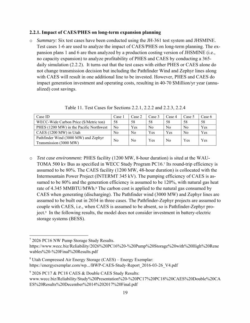
o Summary: Six test cases have been conducted using the JH-361 test system and JHSMINE. Test cases 1-6 are used to analyze the impact of CAES/PHES on long-term planning. The ex-pansion plans 1 and 6 are then analyzed by a production costing version of JHSMINE (i.e., no capacity expansion) to analyze profitability of PHES and CAES by conducting a 365-daily simulation (2.2.2). It turns out that the test cases with either PHES or CAES alone do not change transmission decision but including the Pathfinder Wind and Zephyr lines along with CAES will result in one additional line to be invested. However, PHES and CAES do impact generation investment and operating costs, resulting in 40-70 $Million/yr year (annu-alized) cost savings.

Table 11. Test Cases for Sections 2.2.1, 2.2.2 and 2.2.3, 2.2.4

Case ID Case 1 Case 2 Case 3 Case 4 Case 5 Case 6 WECC-Wide Carbon Price ($/Metric ton) 58 58 58 58 58 58 PHES (1200 MW) in the Pacific Northwest No Yes No No No Yes CAES (1200 MW) in Utah No No Yes Yes No Yes Pathfinder Wind (3000 MW) and Zephyr Transmission (3000 MW)

No No Yes No Yes Yes

o Test case environment: PHES facility (1200 MW, 8-hour duration) is sited at the WAU-TOMA 500 kv Bus as specified in WECC Study Program PC16.7 Its round-trip efficiency is assumed to be 80%. The CAES facility (1200 MW, 48-hour duration) is collocated with the Intermountain Power Project (INTERMT 345 kV). The pumping efficiency of CAES is as-sumed to be 80% and the generation efficiency is assumed to be 120%, with natural gas heat rate of 4.345 MMBTU/MWh.8 The carbon cost is applied to the natural gas consumed by CAES when generating (discharging). The Pathfinder wind (3000 MW) and Zephyr lines are assumed to be built out in 2034 in three cases. The Pathfinder-Zephyr projects are assumed to couple with CAES, i.e., when CAES is assumed to be absent, so is Pathfinder-Zephyr pro-ject.9 In the following results, the model does not consider investment in battery-electric storage systems (BESS).

7 2026 PC16 NW Pump Storage Study Results. https://www.wecc.biz/Reliability/2026%20PC16%20-%20Pump%20Storage%20with%20High%20Renewables%20-%20Final%20Results.pdf 8 Utah Compressed Air Energy Storage (CAES) – Energy Exemplar: https://energyexemplar.com/wp.../BWP-CAES-Study-Report_2016-03-26_V4.pdf 9 2026 PC17 & PC18 CAES & Double CAES Study Results: www.wecc.biz/Reliability/Study%20Presentation%20-%20PC17%20PC18%20CAES%20Double%20CAES%20Results%20December%2014%202017%20Final.pdf

20

o Cost Savings: A detailed cost comparison among all 6 test cases, as well as the resulting mixes of transmission and generation investments are shown in the next two tables below. The major conclusions are as follows. The investigated storage facilities can provide benefits to the system, mainly by lowering carbon costs in operations, and lowering generation invest-ment costs by providing capacity to meet reliability and reserve goals, substituting for gas-fired combustion turbine. By comparing Cases 1 and 2 (with/without PHES), we can con-clude that the PHES alone can provide 13 Million $/yr of benefits to the system (from 2034 and beyond). By comparing Case 1 and Case 4 (with/without CAES, no Pathfinder), we can conclude CAES alone can provide 40 Million $/yr to the system. The existence of a carbon price together CAES’s use of natural gas, results in less usage of CAES and PHES.

o CAES and Pathfinder Wind: By comparing Case 1 and Case 3 (with/without CAES and Path-finder project), we can conclude that this coupled project can provide 2.80 billion $/yr to the system. The cost saving is mostly composed of savings from cheap wind energy, and a re-duced RPS alternative compliance penalty. The latter is a result of Pathfinder making up for a lack of utility scale renewable energy candidates in California.

o Additive Effect: By comparing Case 1-6 altogether, we can conclude that the benefits from PHES, CAES and Pathfinder is additive, i.e., the sum of the cost saving from any individual projects equals the cost saving from implementing them together. Therefore, their benefits can be quantified one project at a time, and it is not necessary to consider all possible combi-nations.

o Emissions: Row 4 in Table 12 indicates that PHES and Pathfinder wind can lower the emis-sions costs by 0.007 B$/yr to 0.44B$/yr. With a carbon price of 58$/Metric ton, this trans-lates to 0.12-7.57 Million Metric tons/yr.

Table 12. Annualized Cost Comparison of Test Cases 1-6 (Annualized Cost, Million $/yr, nega-

tive values represent cost reductions)

Cost Component/Case code name

Incremental relative to Case 1 Case 1 Case 2 Case 3 Case 4 Case 5 Case 6

Generation Expansion 5932 -1 83 -66 154 82 Transmission Expansion 367 0 7 0 7 7

Carbon Cost 8164 -7 -432 4 -439 -435 Variable O&M Cost 2787 1 -107 4 -110 -107

Fuel Cost 14821 -11 -706 10 -713 -725 Fixed O&M Cost 8154 19 177 5 174 196 Unit Commitment

(Start-Up, Shut-Down)155 -14 7 -16 22 -3

RPS Penalty 4082 0 -1828 18 -1850 -1828 TOTAL 44462 -13 -2797 -40 -2755 -2811

21

Table 13. Investment Comparison of Test Cases 1-6 (GW in the Year 2026, online in Year 2034)

Investment Type/ Case code Name

Incremental relative to Case 1

Case 1 Case 2 Case 3 Case 4 Case 5 Case 6

WREZ Lines 46

(22 Lines)0

3 (1 line)*

0 3

(1 line)* 3

(1 line)*

Backbone Reinforcement 8.91

(5 Lines)0 0 0 0 0

Biomass 0.41 0.00 0.00 0.00 0.00 0.00Geothermal 1.76 0.00 0.00 0.00 0.00 0.00

Solar PV with Fixed Tilt 16.98 0.00 1.57 -0.33 1.94 1.57Onshore Wind Generation 21.70 0.00 0.00 0.00 0.00 0.00

Gas CCGT 2.65 -0.03 -0.24 0.00 -0.22 -0.28Gas CT 11.55 0.03 -0.33 -0.56 0.23 -0.30

*This line is an interconnector from WREZ zone 05 (AZ_WE) to Palo Verde (500 kV bus, 15021)

2.2.2 Impact of CAES and PHES on the prices

o Summary: By conducting a 365-day simulation of the generation investments and expanded transmission system in Case 1, Case 2 and Case 4, the JHSMINE team investigated the individual impact of CAES/PHES on the price signals, including LMPs on the facility installation bus, operating reserve prices in sharing region, and capacity payment rate in planning reserve region. The result shows that the installation of CAES/PHES has impact of compressing the volatility.

o Test environment: Three 365-day simulations are conducted using the production cost model module of JHSMINE. The generation and transmission fleets are assumed to be the expanded system resulting from Case 1, Case 2 and Case 4 above. A 365-day simulation is defined as a 24-hour dispatch with unit commitment, repeated for every day in 2034. Note that storages and unit commitment are modeled as the “snake-bite-tail manner,” i.e., the status of generators and storages are assumed to be the same at the beginning and the end of the day. This will understate the value of storage, at least slightly, because it may be optimal to operate storage so that the energy in storage at the end of the day is not the same as at the start of the day, which results in energy being transferred among days and not just among hours within a day.10 A carbon price of $58/Metric ton is applied.

o Price Compression on capacity payment rate: As in Table 12, major benefit to the system from CAES are through savings of generation expansion costs, however, as shown in Table 14, adding CAES at a capacity of 1.2 GW will decrease the capacity payment rate to zero. Thus, a full-size CAES facility will not realize through revenues the full value that it brings to the market, in terms of resource adequacy.

10 A comparison between model intraday operation only and looking 7 days ahead will also be provided in the next section.

22

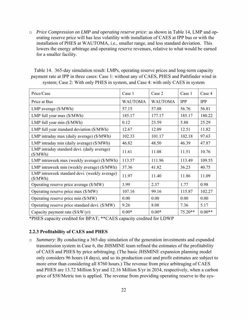
o Price Compression on LMP and operating reserve price: as shown in Table 14, LMP and op-erating reserve price will has less volatility with installation of CAES at IPP bus or with the installation of PHES at WAUTOMA, i.e., smaller range, and less standard deviation. This lowers the energy arbitrage and operating reserve revenues, relative to what would be earned for a smaller facility.

Table 14. 365-day simulation result: LMPs, operating reserve prices and long-term capacity payment rate at IPP in three cases: Case 1: without any of CAES, PHES and Pathfinder wind in

system; Case 2: With only PHES in system, and Case 4: with only CAES in system

Price/Case Case 1 Case 2 Case 1 Case 4

Price at Bus WAUTOMA WAUTOMA IPP IPP

LMP average ($/MWh) 57.15 57.08 56.76 56.81

LMP full year max ($/MWh) 185.17 177.17 185.17 180.22

LMP full year min ($/MWh) 0.12 23.59 5.88 25.29

LMP full year standard deviation ($/MWh) 12.67 12.09 12.51 11.82

LMP intraday max (daily average) ($/MWh) 102.33 101.17 102.18 97.63

LMP intraday min (daily average) ($/MWh) 46.82 48.50 46.39 47.87 LMP intraday standard devi. (daily average) ($/MWh)

11.61 11.08 11.51 10.76

LMP intraweek max (weekly average) ($/MWh) 113.57 111.96 113.49 109.55

LMP intraweek min (weekly average) ($/MWh) 37.36 41.82 36.23 40.75 LMP intraweek standard devi. (weekly average) ($/MWh)

11.97 11.40 11.86 11.09

Operating reserve price average ($/MW) 3.99 2.37 1.77 0.98

Operating reserve price max ($/MW) 107.16 99.16 115.87 102.27

Operating reserve price min ($/MW) 0.00 0.00 0.00 0.00

Operating reserve price standard devi. ($/MW) 9.26 8.08 7.36 5.17

Capacity payment rate ($/kW/yr) 0.00* 0.00* 75.20** 0.00**

*PHES capacity credited for BPAT; **CAES capacity credited for LDWP

2.2.3 Profitability of CAES and PHES

o Summary: By conducting a 365-day simulation of the generation investments and expanded transmission system in Case 6, the JHSMINE team refined the estimates of the profitability of CAES and PHES by price arbitraging. (The basic JHSMINE expansion planning model only considers 96 hours (4 days), and so its production cost and profit estimates are subject to more error than considering all 8760 hours.) The revenue from price arbitraging of CAES and PHES are 13.72 Million $/yr and 12.16 Million $/yr in 2034, respectively, when a carbon price of $58/Metric ton is applied. The revenue from providing operating reserve to the sys-

23

tem of CAES and PHES are 5.51 Million $/yr and 15.55 Million $/yr. The sums of the reve-nues are significantly lower than the associated cost reductions: sum of annualized capital cost, fixed cost and fuel cost. See detailed numerical results below. This can occur because the size of the CAES and PHES facilities can result in a decline in day-night price differences at their buses relative to the situation without those facilities. CAES is miss its payment by providing capacity to the California-South region because the size of CAES diminishes the capacity payment rate to zero, see details in the previous section.

o Test environment: A 365-day simulation is conducted using the production cost model mod-ule of JHSMINE. The generation and transmission fleets are assumed to be the expanded system resulting from “Planning 2034 with CAES/PHES (Case 6)” above. A 365-day simula-tion is defined as a 24-hour dispatch with unit commitment, repeated for every day in 2034. Note that storages and unit commitment are modeled as the “snake-bite-tail manner,” i.e., the status of generators and storages are assumed to be the same at the beginning and the end of the day. This will understate the value of storage, at least slightly, because it may be optimal to operate storage so that the energy in storage at the end of the day is not the same as at the start of the day, which results in energy being transferred among days and not just among hours within a day. A carbon price of $58/Metric ton is applied.

o Operation Duration Curve: The operation duration curve of PHES and CAES can be found below. It shows that PHES is operated much more expensively than CAES.

Figure 5. Charge and discharge duration curve of CAES/PSES (Positive: Generation)

o Revenue from price arbitrage and operating reserve: JHSMINE team defines the revenue of price arbitrage as the revenue if the storage pumps, buying at the locational marginal price of the located bus, and sells its generation also at the LMP of its bus. JHSMINE team defines the revenue of providing operating reserve as selling the reserved capacity (head room) to the des-ignated reserve region: CAES sells reserved spinning capacity to CA-South, and PHES to

‐1500

‐1000

‐500

0

500

1000

1500

1

251

501

751

1001

1251

1501

1751

2001

2251

2501

2751

3001

3251

3501

3751

4001

4251

4501

4751

5001

5251

5501

5751

6001

6251

6501

6751

7001

7251

7501

7751

8001

8251

8501

8751

CAES PHES

24

Northwest Power Pool (NWPP). For storages to provide the operating reserve, the state of charge of the storage at the beginning of the hour should be at least enough for a half hour if the reserve is called, excluding the scheduled discharging energy; if a storage is charging, the charging capacity is automatically accounted for operating reserve. A comparison of revenue of price arbitrage, providing operating reserve and costs associated with the storage facilities can be found below. This shows that the revenue is of the same order of magnitude as the variable costs and is far short of the annual capital cost.

Table 15. Annual (52 weeks) Cost and Benefit of CAES and PSES ($Million/yr), Carbon price $58/Metric ton, transmission and generation fleets expanded as in Case 6

Storage CAES (1200 MW) in IPP PHES (1200 MW) in the PW

Revenue of Price Arbitrage 13.72 12.16

Revenue of Providing Operating Reserve 5.51 15.55

Fixed O&M 17.38 18.90

Fuel Cost and carbon cost 9.27 0.00

Annualized Capital Cost 118.89 174.83

o Impact of looking-ahead: as stated above, looking only at intraday difference might underesti-mate the profitability of CAES and PHES. Thus a separate analysis is conducted by building a storage operations simulation model (in contrast to JHSMINE, a system wide planning/dis-patch simulation model). This model 1) uses as an input the 8760 hours of local prices from the JHSMINE 365 daily simulation for the respectively buses where CAES and PHES are located and 2) optimizes the operating of the storage again by looking ahead 1-day, 7-days or longer. The following table shows the results of the production costing model (dispatch only, fixed generation and transmission plant) including the operating reserve requirement. The ta-ble compares the impact of “looking ahead” 1 day (only intraday benefit is captured) versus 7 full day look-ahead or longer (in the extreme case, looking ahead for the full 8760 hours sim-ulated for 2034). Carbon price is $58/metric ton. We note that there are alternative dispatches that are equally profitable for CAES/PHES. In particular, under the 365 day simulation, it is equally profitable to provide energy arbitrage and operating reserves on many days because operating reserve prices are being set by the opportunity cost of energy provided by CAES/PHES. The most important result is the total Gross Margin. Compared to looking 7 days ahead, 1-day modeling (intraday price differences only) will miss 22.3% of profit of CAES (about $2.85M/year) and 9% of profit of PHES (about $2.74M /year).

25

Table 16. 2034-yearly profit ($M/yr) of CAES in Case 6 (with CAES, PHES and Pathfinder wind installed) in different look-ahead schemes: Storage operations model based on simulated prices

from JHSMINE 365 Day operations model

Price Arbitrage Revenue

Operating Reserve Revenue

Operating Cost

Total Gross Margin

1-Day optimization (for each of 365 days)

13.72 5.51 9.27 9.96

Alternative optimum for 1-Day optimization (365 days) by purely storage operation

simulation

25.70 1.35 17.10 9.96

Optimization over 7 days (52 periods)

27.78 3.39 18.36 12.81


28.67 3.54 19.02 13.20


29.58 3.62 18.37 14.83

Optimization over 365 days (1 period)

29.14 3.65 17.92 14.87

Table 17. 2034-yearly profit ($M/yr) of PHES in Case 6 (with CAES, PHES and Pathfinder wind installed) in different look-ahead scheme.



Total Gross Margin

1-Day optimization (for each of 365 days) 12.16 15.55 27.71 Alternative optimum for 1-Day optimization

(365 days) by purely storage operation simula-tion

11.03 16.68 27.71

Optimization over 7 days (52 periods) 15.89 14.56 30.45



Optimization over 365 days (1 period) 16.03 14.68 30.71

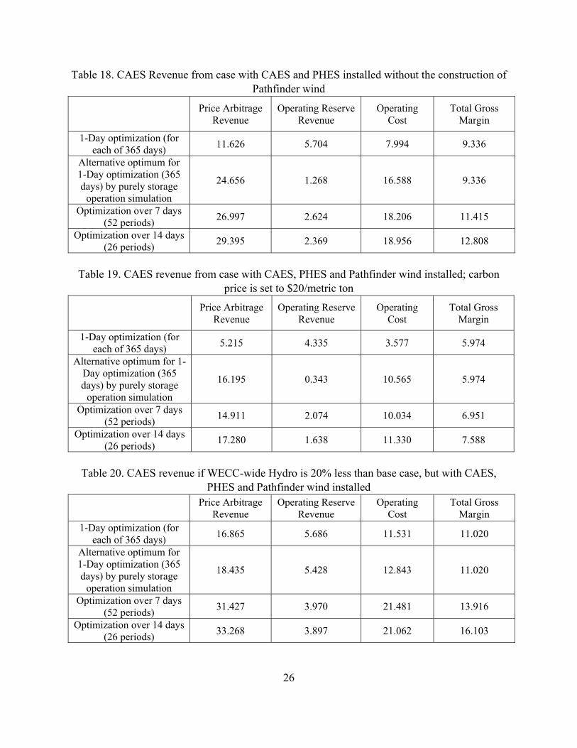
o Sensitivity Analysis of CAES profitability: the impacts of the Pathfinder wind installation, the carbon price (set to $20/metric ton), and the hydroelectricity availability (WECC hydro is down scaled to 80%) on the CAES profitability are investigated. In particular for hydro sen-sitivity, we assume we plan our power system as hydro is medium year (2009) but the really hydro profiles are 80% lower WECC-wide, for the whole year. The result shows that 1) Path-finder wind is making the profit of CAES higher. The profit from “looking-7-day” ahead run is raised $1.4 million/year, about 12.3%, compared to CAES without Pathfinder Wind; 2) a carbon price of $58/metric ton makes the profit of CAES higher; 3) 20% lower hydro availa-bility makes the gross margins of CAES about 20% higher.

26

Table 18. CAES Revenue from case with CAES and PHES installed without the construction of Pathfinder wind



Operating Cost

Total Gross Margin


11.626 5.704 7.994 9.336

Alternative optimum for 1-Day optimization (365 days) by purely storage

operation simulation

24.656 1.268 16.588 9.336


26.997 2.624 18.206 11.415


29.395 2.369 18.956 12.808

Table 19. CAES revenue from case with CAES, PHES and Pathfinder wind installed; carbon

price is set to $20/metric ton



Operating Cost

Total Gross Margin


5.215 4.335 3.577 5.974



16.195 0.343 10.565 5.974


14.911 2.074 10.034 6.951


17.280 1.638 11.330 7.588

Table 20. CAES revenue if WECC-wide Hydro is 20% less than base case, but with CAES,

PHES and Pathfinder wind installed



Operating Cost

Total Gross Margin


16.865 5.686 11.531 11.020



18.435 5.428 12.843 11.020


31.427 3.970 21.481 13.916


33.268 3.897 21.062 16.103

27

2.2.4 Impact of PHES/CAES on congestion in 2034

o Summary: The JHSMINE team investigated the impact of PHES/CAES on congestion in 2034 by comparing path utilization differences between the 365-daily simulations of Cases 1 and 6, above.

o Path Utilization: Path utilization comparisons of Cases 1 and 6 are shown in Figure 6, Figure 7, and Figure 8. Only the Paths with significant differences (>1%) in terms of utilization metric 99 (U99) are shown. Our Path Utilization definition is aligned in the WECC-study case: for one path, the utilization is the percentage of the hours that the path flow is above a threshold level relative to the path limit.11 Noted that backbone candidates in JH-361 can be invested in to raise the path limit. Such updated paths are Path 1, 3, 31, 45.

o Numerical Results:

Remark 1: PHES/CAES/Pathfinder has a great impact upon Path 27 (Intermountain Power Project DC Line) and Path 28 (Intermountain-Mona 345 kV). For Path 27, the utilization is greatly increased because of the WIND/Storage installation. For Path 28, the impact makes the utilization less.

Remark 2: The utilization of multiple Paths that are not nearby the installed storage/wind has changed, showing the impact of investigated facilities can be distance-independent. For example, the utilization of Path 1 (Alberta-British Columbia) is significantly higher when the storage/wind options are installed (Case 6).

11 2026 PC17 & PC18 CAES & Double CAES Study Results, found in www.wecc.biz/Reliability/Study%20Presentation%20-%20PC17%20PC18%20CAES%20Double%20CAES%20Results%20December%2014%202017%20Final.pdf.

For example, U99 of one path is calculated as the following steps. 1) For that path, identify how many hours in a year when the path flows are above 99% of the path limits. If a path limit is 10,000 MW in both directions, then count the hours where path flows are above 99%*10,000 MW = 9900 MW. Say X is the result. 2) U99 of that path is calculated as X/8760. For U75 and U90, the thresholds are 75% and 90%, respectively.

28

Table 21. Preserved Paths in JH-361

Path Name Path Name

P01 Alberta-British Columbia P38 TOT 4B

P03 Northwest-British Columbia P39 TOT 5

P04 West of Cascades-North P42 IID-SCE

P05 West of Cascades-South P45 SDG&E-CFE

P06 West of Hatwai P46 West of Colorado River (WOR)

P08 Montana to Northwest P47 Southern New Mexico (NM1)

P14 Idaho to Northwest P48 Northern New Mexico (NM2)

P15 Midway-LosBanos P49 East of Colorado River (EOR)

P16 Idaho-Sierra P55 Brownlee East

P17 Borah West P58 Eldorado-Mead 230 kV Lines

P18 Montana-Idaho P61 Lugo-Victorville 500 kV Line

P19 Bridger West P62 Eldorado-McCullough 500 kV Line

P20 Path C P65 Pacific DC Intertie (PDCI)

P22 Southwest of Four Corners P66 COI

P26 Northern-Southern California P71 South of Allston

P27 Intermountain Power Project DC Line P73 North of John Day

P28 Intermountain-Mona 345 kV P75 Hemingway-Summer Lake

P29 Intermountain-Gonder 230 kV P76 Alturas Project

P30 TOT 1A P77 Crystal-Allen

P31 TOT 2A P78 TOT 2B1

P32 Pavant-Gonder InterMtn-Gonder 230 kV P79 TOT 2B2

P33 Bonanza West P81 Southern Nevada Transmission Interface (SNIT)

P35 TOT 2C P82 TotBeast

P37 TOT 4A P83 Montana Alberta Tie Line

29

Figure 6. Path Utilization (U75) in 2034, a comparison between Case 1 (without CAES/PHES/Pathfinder) and Case 6 (with CAES/PHES/Pathfinder); Paths with U75 lower than

15% in both Case 1 and 6 NOT shown



0.00%

10.00%

20.00%

30.00%

40.00%

50.00%

60.00%

70.00%

80.00%

90.00%

100.00%

P1

P4

P8

P14

P15

P16

P18

P20

P22

P26

P27

P28

P29

P30

P31

P32

P33

P35

P39

P45

P47

P48

P58

P61

P62

P65

P66

P71

P75

P76

P78

P79

P83

Case 1 Case 6

0.00%

10.00%

20.00%

30.00%

40.00%

50.00%

60.00%

70.00%

80.00%

90.00%

100.00%

P1

P4

P14

P15

P16

P18

P20

P22

P26

P27

P28

P29

P30

P31

P32

P33

P35

P39

P45

P47

P48

P58

P61

P62

P65

P66

P71

P75

P76

P79

P83

Case 1 Case 6

30



2.3 Comparison of the base and alternative cases to determine the interaction of storage, transmission economics, and renewable integration

In this part, we demonstrate the interaction of storage, transmission and generation expansion by conducting analyses for several test cases: generation, transmission and storage expansion co-optimization with various carbon price and storage costs. The target is to answer the following question: Under what circumstances can the option of storage expansion change the transmis-sion and generation expansion and the WECC system? An analysis road map can be found be-low.

Figure 9. Analysis Road Map for Section 2.3

0

0.1

0.2

0.3

0.4

0.5

0.6

0.7

0.8

0.9

P1

P4

P14

P15

P16

P18

P20

P22

P26

P27

P28

P29

P30

P31

P32

P33

P35

P37

P39

P45

P47

P48

P58

P61

P62

P65

P66

P71

P75

P76

P79

P83

Case 1 Case 6

Enabling Storage Investment in JHSMINE

Add BESS Candidates on all existing buses and WREZ hubs

•10 test cases are constructed using different carbon prices and storage capital cost

Planning for 2034

•Output 1: Cost savings for 2034

•Output 2: Generation/ transmission/ storage expansion plan for 2034

31

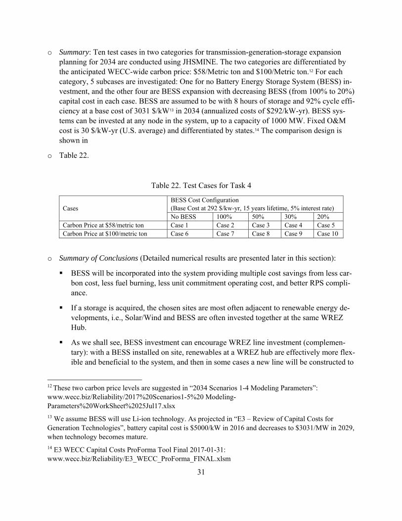
o Summary: Ten test cases in two categories for transmission-generation-storage expansion planning for 2034 are conducted using JHSMINE. The two categories are differentiated by the anticipated WECC-wide carbon price: $58/Metric ton and $100/Metric ton.12 For each category, 5 subcases are investigated: One for no Battery Energy Storage System (BESS) in-vestment, and the other four are BESS expansion with decreasing BESS (from 100% to 20%) capital cost in each case. BESS are assumed to be with 8 hours of storage and 92% cycle effi-ciency at a base cost of 3031 $/kW13 in 2034 (annualized costs of $292/kW-yr). BESS sys-tems can be invested at any node in the system, up to a capacity of 1000 MW. Fixed O&M cost is 30 $/kW-yr (U.S. average) and differentiated by states.14 The comparison design is shown in

o Table 22.

Table 22. Test Cases for Task 4

Cases BESS Cost Configuration (Base Cost at 292 $/kw-yr, 15 years lifetime, 5% interest rate) No BESS 100% 50% 30% 20%

Carbon Price at $58/metric ton Case 1 Case 2 Case 3 Case 4 Case 5 Carbon Price at $100/metric ton Case 6 Case 7 Case 8 Case 9 Case 10

o Summary of Conclusions (Detailed numerical results are presented later in this section):

BESS will be incorporated into the system providing multiple cost savings from less car-bon cost, less fuel burning, less unit commitment operating cost, and better RPS compli-ance.

If a storage is acquired, the chosen sites are most often adjacent to renewable energy de-velopments, i.e., Solar/Wind and BESS are often invested together at the same WREZ Hub.

As we shall see, BESS investment can encourage WREZ line investment (complemen-tary): with a BESS installed on site, renewables at a WREZ hub are effectively more flex-ible and beneficial to the system, and then in some cases a new line will be constructed to

12 These two carbon price levels are suggested in “2034 Scenarios 1-4 Modeling Parameters”: www.wecc.biz/Reliability/2017%20Scenarios1-5%20 Modeling-Parameters%20WorkSheet%2025Jul17.xlsx 13 We assume BESS will use Li-ion technology. As projected in “E3 – Review of Capital Costs for Generation Technologies”, battery capital cost is $5000/kW in 2016 and decreases to $3031/MW in 2029, when technology becomes mature. 14 E3 WECC Capital Costs ProForma Tool Final 2017-01-31: www.wecc.biz/Reliability/E3_WECC_ProForma_FINAL.xlsm

32

deliver the additional renewable power to the system. See WREZ hub 19 in Case 4 (Table 25) and 9 (Table 26).

In contrast, BESS investment can discourage Backbone line investment (substitution): with a BESS installed nearby, there is a case in which a backbone reinforcement project that was selected without BESS is canceled (i.e., no longer built).

o Numerical Results:

A cost comparison between each 5 cases is shown in the next two tables: they show that the cost savings from BESS, when installed, derive from lowering carbon costs, less fuel burn costs, fewer start-ups/shut downs of conventional generation units, and better re-newable accommodation (lower RPS alternative compliance penalty).

Cost comparisons between cases with different carbon prices show that, generally, higher carbon cost will incentive system to invest slightly more in BESS.

Table 23. Cost Comparison of Cases 1-5, Carbon Price $58/Metric ton, 100% BESS cost =

$292/kW-yr (Annualized Cost, Billion $/yr)

Cost Component Case 1:

NO BESS

Case 2: 100%

BESS Cost

Case 3: 50% BESS

Cost

Case 4: 30% BESS

Cost

Case 5: 20% BESS

Cost

Generation Expansion Cost 5.93 6.17 6.29 6.06 5.69 Energy Storage Investment Cost 0.00 0.46 0.60 0.67 0.77 Transmission Expansion Cost 0.37 0.37 0.38 0.37 0.37 Carbon Cost 8.16 8.01 7.88 7.83 7.77 Variable O&M Cost 2.79 2.75 2.72 2.72 2.72 Fuel Cost 14.82 14.56 14.41 14.35 14.28 Fixed O&M Cost 8.15 8.27 8.38 8.45 8.58 Start-up/Shut-down Cost 0.15 0.16 0.15 0.11 0.07 RPS Noncompliance Penalty 4.08 3.63 3.19 3.14 3.14 Total Cost 44.46 44.38 44.00 43.71 43.40 Cost Without BESS Investment Cost 44.46 43.92 43.40 43.04 42.62 Gross Benefit* 0.00 0.54 1.06 1.42 1.84 Benefit/Cost Ratio - 117.63% 177.92% 212.17% 238.02%

*Gross Benefit is defined by the differences of “system costs without BESS capital cost” (row 11) between any case and case 1.

33

Table 24. Cost Comparison between Case 6-10, Carbon Price $100/Metric ton, 100% BESS cost = $292/kW-yr (Annualized Cost, Billion $/yr)

Cost Component Case 6:

NO BESS

Case 7: 100%

BESS Cost

Case 8: 50% BESS

Cost

Case 9: 30% BESS

Cost

Case 10: 20% BESS

Cost

Generation Expansion Cost 8.15 8.27 8.32 8.02 8.18 Energy Storage Investment Cost 0.00 0.69 0.62 0.74 1.01 Transmission Expansion Cost 0.51 0.51 0.51 0.50 0.52 Carbon Cost 12.23 12.02 11.91 11.85 11.39 Variable O&M Cost 2.60 2.57 2.56 2.56 2.50 Fuel Cost 13.17 12.97 12.88 12.84 12.36 Fixed O&M Cost 8.82 8.94 9.00 9.11 9.47 Start-up/Shut-down Cost 0.41 0.38 0.38 0.27 0.16 RPS Noncompliance Penalty 4.08 3.45 3.18 3.14 3.09 Total Cost 49.97 49.82 49.37 49.05 48.68 Cost Without BESS Investment Cost 49.97 49.13 48.75 48.31 47.67 Gross Benefit* 0.00 0.84 1.22 1.66 2.30 Benefit/Cost Ratio - 122.27% 196.64% 223.31% 226.86%

*Gross Benefit is defined by the differences of “system costs without BESS capital cost” (row 11) between any case and case 1.

WECC-wide generation production mix for Case 1, Case 4, Case 6 and Case 9 can be found in Figure 10. The results are showing 1) the carbon price of $58/metric ton or higher elim-inates the coal production; 2) the storage installation is increasing the proportion of Solar in the generation production mix.

34

Figure 10. WECC-wide generation production mix for Cases 1, 4, 6 and 9 (Year 2034 TWh)

WECC-wide generation, transmission and storage expansion plans are shown in different cases summarized below. Generation and storage expansion and associated carbon inten-sity (defined as total emission in 2034 divided by total energy consumed) are shown in Figure 11 and Figure 12. We make three remarks:

The installation of storage incentivizes more solar capacity.

The installation of storage can lower the carbon intensity of the WECC system, even when there is already a high carbon price introduced by aggressive carbon policies.

-50.00 0.00 50.00 100.00 150.00 200.00 250.00 300.00 350.00

BIO

BIO-NEW

COAL

DG-BTM

EE

CCGT

CCGT-NEW

CT

CT-NEW

GEO

GEO-NEW

HYDRO

HYDRO-RPS

MOTORLOAD

NUCLEAR

PS-HYDRO

PVF

PFV-NEW

PVT

CSP

ST-OTHER

WIND

WIND-NEW

Case 1 Case 4 Case 6 Case 9

35

When the BESS cost is 30% percent of the baseline level, the substitution effect from natural gas combustion turbines (CT) to BESS become significant. CT is a major source of planned reserve and reliability goals (see 2.1.2 above) because of its low capital cost and high (near to 1) expected load carrying capability (ELCC). BESS’s ELCC in JHSMINE/LTPT is also set to 1; at a cost that is 30% of the base level, it becomes more attractive than CTs for meeting reserve requirements, given that it also provides value in the form of storage services.

Figure 11. Cases 1-5: Generation capacity and storage additions in 2034 (GW, left axis), and car-bon intensity (metric T/GWh, red dashes, right axis), carbon price = $58/Metric ton

122.00

123.00

124.00

125.00

126.00

127.00

128.00

129.00

130.00

0.00

5.00

10.00

15.00

20.00

25.00

NO BESS 100% BESS Cost 50% BESS Cost 30% BESS Cost 20% BESS CostBIO-NEW (GW) CCGT-NEW (GW) CT-NEW (GW)GEO-NEW (GW) PVF-NEW (GW) WIND-NEW (GW)

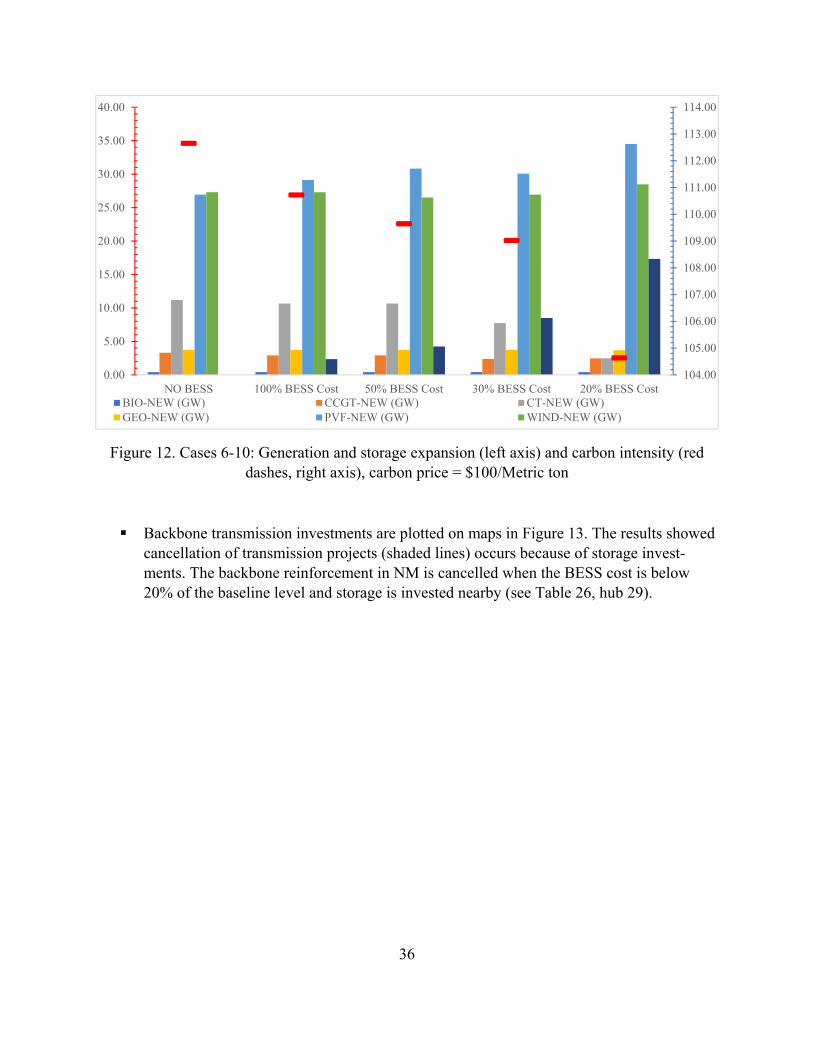
36

Figure 12. Cases 6-10: Generation and storage expansion (left axis) and carbon intensity (red dashes, right axis), carbon price = $100/Metric ton

Backbone transmission investments are plotted on maps in Figure 13. The results showed cancellation of transmission projects (shaded lines) occurs because of storage invest-ments. The backbone reinforcement in NM is cancelled when the BESS cost is below 20% of the baseline level and storage is invested nearby (see Table 26, hub 29).

104.00

105.00

106.00

107.00

108.00

109.00

110.00

111.00

112.00

113.00

114.00

0.00

5.00

10.00

15.00

20.00

25.00

30.00

35.00

40.00

NO BESS 100% BESS Cost 50% BESS Cost 30% BESS Cost 20% BESS CostBIO-NEW (GW) CCGT-NEW (GW) CT-NEW (GW)GEO-NEW (GW) PVF-NEW (GW) WIND-NEW (GW)

37

Figure 13. Backbone Reinforcements in Case 1-5 (left) and Case 6-10 (right). Red-circled line is cancelled when BESS cost is 20% of baseline level

Investments in WREZ hub-level renewable generation investment (map shown in Figure 14), and renewable connections are shown in the next table, where hub rows that have different results between Cases 1 and 4 are highlighted in yellow, and changes in trans-mission are highlighted in red. At hub 19, we can see that with BESS installed, more WREZ transmission is built because more renewable generation is installed. In the bot-tom row, we can see that with BESS installed, more solar and slightly less wind is built. Total BESS investment is around 7.64 GW (Figure 11) of which 5.38 GW (bottom row) is either located “on site” (at the WREZ hub) or at the other end of a WREZ transmission line (where it connects with the grid). At hubs 1 and 50, a BESS system is installed purely for better operation of the wind turbines, since there is no additional renewable in-stallation and new additional transmission investment (Case 4 versus Case 1). Results also show a substitute relationship between BESS and transmission investment, e.g., when batteries become cheap, then a WREZ transmission interconnector (0.8GW) is can-celed on Hub 1, and a storage was put at the WREZ hub.

Similar results for Case 6 and Case 9 can be found in Table 26. With a more aggressive carbon price in place, more renewables are installed compared to Case 1 and 4. More

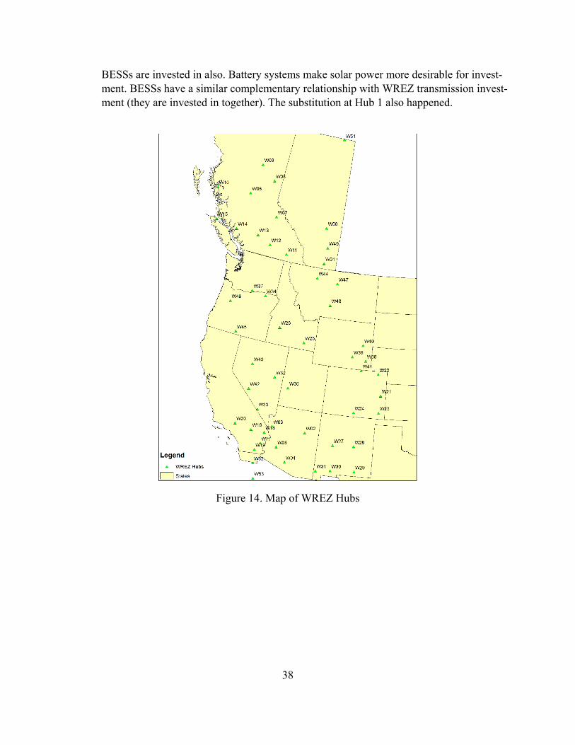
38

BESSs are invested in also. Battery systems make solar power more desirable for invest-ment. BESSs have a similar complementary relationship with WREZ transmission invest-ment (they are invested in together). The substitution at Hub 1 also happened.

Figure 14. Map of WREZ Hubs

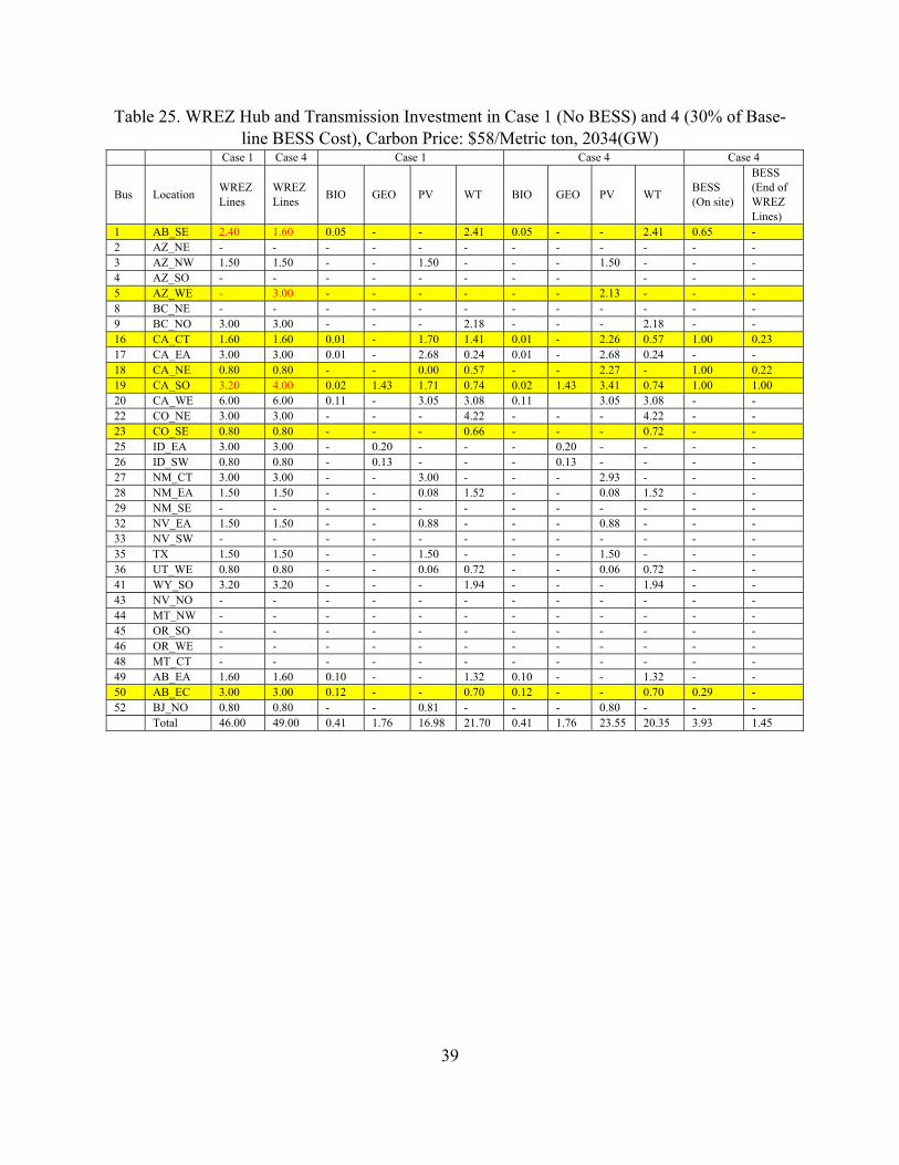
39

Table 25. WREZ Hub and Transmission Investment in Case 1 (No BESS) and 4 (30% of Base-line BESS Cost), Carbon Price: $58/Metric ton, 2034(GW)

Case 1 Case 4 Case 1 Case 4 Case 4

Bus Location WREZ Lines

WREZ Lines

BIO GEO PV WT BIO GEO PV WT BESS (On site)

BESS (End of WREZ Lines)

1 AB_SE 2.40 1.60 0.05 - - 2.41 0.05 - - 2.41 0.65 - 2 AZ_NE - - - - - - - - - - - - 3 AZ_NW 1.50 1.50 - - 1.50 - - - 1.50 - - - 4 AZ_SO - - - - - - - - - - - 5 AZ_WE - 3.00 - - - - - - 2.13 - - - 8 BC_NE - - - - - - - - - - - - 9 BC_NO 3.00 3.00 - - - 2.18 - - - 2.18 - - 16 CA_CT 1.60 1.60 0.01 - 1.70 1.41 0.01 - 2.26 0.57 1.00 0.23 17 CA_EA 3.00 3.00 0.01 - 2.68 0.24 0.01 - 2.68 0.24 - - 18 CA_NE 0.80 0.80 - - 0.00 0.57 - - 2.27 - 1.00 0.22 19 CA_SO 3.20 4.00 0.02 1.43 1.71 0.74 0.02 1.43 3.41 0.74 1.00 1.00 20 CA_WE 6.00 6.00 0.11 - 3.05 3.08 0.11 3.05 3.08 - - 22 CO_NE 3.00 3.00 - - - 4.22 - - - 4.22 - - 23 CO_SE 0.80 0.80 - - - 0.66 - - - 0.72 - - 25 ID_EA 3.00 3.00 - 0.20 - - - 0.20 - - - - 26 ID_SW 0.80 0.80 - 0.13 - - - 0.13 - - - - 27 NM_CT 3.00 3.00 - - 3.00 - - - 2.93 - - - 28 NM_EA 1.50 1.50 - - 0.08 1.52 - - 0.08 1.52 - - 29 NM_SE - - - - - - - - - - - - 32 NV_EA 1.50 1.50 - - 0.88 - - - 0.88 - - - 33 NV_SW - - - - - - - - - - - - 35 TX 1.50 1.50 - - 1.50 - - - 1.50 - - - 36 UT_WE 0.80 0.80 - - 0.06 0.72 - - 0.06 0.72 - - 41 WY_SO 3.20 3.20 - - - 1.94 - - - 1.94 - - 43 NV_NO - - - - - - - - - - - - 44 MT_NW - - - - - - - - - - - - 45 OR_SO - - - - - - - - - - - - 46 OR_WE - - - - - - - - - - - - 48 MT_CT - - - - - - - - - - - - 49 AB_EA 1.60 1.60 0.10 - - 1.32 0.10 - - 1.32 - - 50 AB_EC 3.00 3.00 0.12 - - 0.70 0.12 - - 0.70 0.29 - 52 BJ_NO 0.80 0.80 - - 0.81 - - - 0.80 - - -

Total 46.00 49.00 0.41 1.76 16.98 21.70 0.41 1.76 23.55 20.35 3.93 1.45

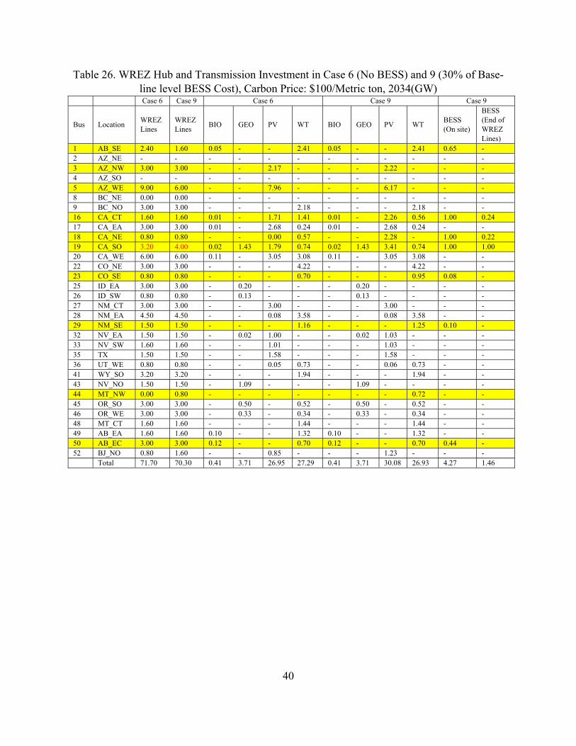
40

Table 26. WREZ Hub and Transmission Investment in Case 6 (No BESS) and 9 (30% of Base-line level BESS Cost), Carbon Price: $100/Metric ton, 2034(GW)

Case 6 Case 9 Case 6 Case 9 Case 9

Bus Location WREZ Lines

WREZ Lines

BIO GEO PV WT BIO GEO PV WT BESS (On site)

BESS (End of WREZ Lines)

1 AB_SE 2.40 1.60 0.05 - - 2.41 0.05 - - 2.41 0.65 - 2 AZ_NE - - - - - - - - - - - - 3 AZ_NW 3.00 3.00 - - 2.17 - - - 2.22 - - - 4 AZ_SO - - - - - - - - - - - - 5 AZ_WE 9.00 6.00 - - 7.96 - - - 6.17 - - - 8 BC_NE 0.00 0.00 - - - - - - - - - - 9 BC_NO 3.00 3.00 - - - 2.18 - - - 2.18 - - 16 CA_CT 1.60 1.60 0.01 - 1.71 1.41 0.01 - 2.26 0.56 1.00 0.24 17 CA_EA 3.00 3.00 0.01 - 2.68 0.24 0.01 - 2.68 0.24 - - 18 CA_NE 0.80 0.80 - - 0.00 0.57 - - 2.28 - 1.00 0.22 19 CA_SO 3.20 4.00 0.02 1.43 1.79 0.74 0.02 1.43 3.41 0.74 1.00 1.00 20 CA_WE 6.00 6.00 0.11 - 3.05 3.08 0.11 - 3.05 3.08 - - 22 CO_NE 3.00 3.00 - - - 4.22 - - - 4.22 - - 23 CO_SE 0.80 0.80 - - - 0.70 - - - 0.95 0.08 - 25 ID_EA 3.00 3.00 - 0.20 - - - 0.20 - - - - 26 ID_SW 0.80 0.80 - 0.13 - - - 0.13 - - - - 27 NM_CT 3.00 3.00 - - 3.00 - - - 3.00 - - - 28 NM_EA 4.50 4.50 - - 0.08 3.58 - - 0.08 3.58 - - 29 NM_SE 1.50 1.50 - - - 1.16 - - - 1.25 0.10 - 32 NV_EA 1.50 1.50 - 0.02 1.00 - - 0.02 1.03 - - - 33 NV_SW 1.60 1.60 - - 1.01 - - - 1.03 - - - 35 TX 1.50 1.50 - - 1.58 - - - 1.58 - - - 36 UT_WE 0.80 0.80 - - 0.05 0.73 - - 0.06 0.73 - - 41 WY_SO 3.20 3.20 - - - 1.94 - - - 1.94 - - 43 NV_NO 1.50 1.50 - 1.09 - - - 1.09 - - - - 44 MT_NW 0.00 0.80 - - - - - - - 0.72 - - 45 OR_SO 3.00 3.00 - 0.50 - 0.52 - 0.50 - 0.52 - - 46 OR_WE 3.00 3.00 - 0.33 - 0.34 - 0.33 - 0.34 - - 48 MT_CT 1.60 1.60 - - - 1.44 - - - 1.44 - - 49 AB_EA 1.60 1.60 0.10 - - 1.32 0.10 - - 1.32 - - 50 AB_EC 3.00 3.00 0.12 - - 0.70 0.12 - - 0.70 0.44 - 52 BJ_NO 0.80 1.60 - - 0.85 - - - 1.23 - - -

Total 71.70 70.30 0.41 3.71 26.95 27.29 0.41 3.71 30.08 26.93 4.27 1.46

41

3. QUALITATIVE ASSESSMENT OF JHSMINE CAPABILITIES TO ADDRESS KEY ISSUES IN PLANNING

This section addresses the second of the two phases of this project. The topics to be addressed in this qualitative assessment include the capability of the JHSMINE tool to address the following considerations in regional transmission planning. These considerations were defined by WECC staff.

1. Public Policy Goals, especially renewable portfolio standards

2. Resource adequacy to meet annual load energy needs

3. Optimal generation modeling capability, including flexibility, least cost dispatch, and se-curity constraints

4. Modeling logic and protocol for evaluating transmission and generation portfolio coopti-mization

5. Reliability considerations including must-run, local and system portfolio and dispatch constraints

6. Multiple generation, transmission, and substation configurations

7. Geospatial considerations

8. Pool constraints

9. Seasonal load variations

A section is devoted to each of these considerations below. In each section, we summarize the model functionalities that planners might desire, and whether and how the present JHSMINE in-cludes those functionalities. If JHSMINE does not have the capability at this time, we describe whether and how a JHSMINE could be revised to do so. We attempt to adhere to WECC termi-nology in discussing each type of functionality.15

Note that we do not discuss the capabilities of JHSMINE to explore the implications of long-run uncertainties (economic, technological, and policy), since those capabilities were thoroughly ex-plored in our previous report.16

15 M. Bailey, "Release Notes – WECC Draft 2034 Reference Case, Accompanies WECC Draft 2034 Reference Case, Version 1.0," WECC System Adequacy Planning (SAP) Department, Salt Lake City, UT, September 16, 2016 16 Ho et al., Footnote 1, supra.

42

3.1 Public Policy Goals: - Ability of the tool to capture policy goals (state RPS, carve-out, tiers)

This concerns the ability of JHSMINE to capture specific features of the renewable portfolio systems in place or potentially adopted in the future by western States and Provinces. These fea-tures include those listed below. For each feature, we summarize whether JHSMINE (present version or future version) can accommodate the feature:

How the requirement is determined (as a fraction of sales within a particular state or other region, most commonly). This is handled in the present JHSMINE by defining a MWh/year requirement, which is calculated based on the assumed load in the relevant re-gion. We have created a mapping of Balancing Areas to states in the WECC region to facilitate definition of these regions (Table 6, above). RPS 2034 goals considered in that version of JHSMINE are shown in Table 7, above.

Whether use of banked credits from previous years and banking of surplus credits is pos-sible. This functionality is not handled in JHSMINE, since accounting is for a single year, and only two operating years (e.g., 2028 and 2038) are represented, without ac-counting for inter-year variability of a resource or precise year of resource additions.

Which types and vintages of resources qualify to provide credits to meet the requirement. Handled in the present JHSMINE by defining which types of generation sources can pro-vide MWh that would be counted. JHSMINE could be easily revised to account for par-tial credits if different types of resources received different credits (multipliers, e.g., as in the case of UK offshore wind, which used to receive two times the credit of UK on-shore wind). The RPS feature in JHSMINE also could be revised to give credit for energy effi-ciency investments (which presently are prespecified by the user and not solved for by the model) or distributed generation not accounted for in the generation optimization by deducting their credits from the MWh requirement

Which locations of resources can be counted, and whether trade with other jurisdictions is allowed. In previous analyses, we have found that restrictions on renewable energy credits trade (RECs) can dramatically change transmission locations, since remote re-sources of high quality are often located in states without their own RPSs, and so REC trade would encourage transmission.17 In our Phase I analyses, no trade was allowed, but users have the option to allow trade between selected jurisdictions or WECC-wide in JHSMINE. JHSMINE creates constraints that trace sales of RECs and ensures that RECs are not double-counted (by an individual resource’s output being used to satisfy more than one jurisdiction’s RPS).

Carve-outs and tiers. These are accounted for in JHSMINE, and are defined mathemati-cally by defining a MWh requirement (see above) and qualifying types, locations, and

17 A.P. Perez, E.E. Sauma, F.D. Munoz, and B.F. Hobbs, “The Economic Effects of Interregional Trading of Renews.able Energy Certificates in the WECC,” The Energy Journal, 37(4), 2016, 267-296.

43

vintages of resources. For instance, solar might have its own RPS, but solar resources might also count towards a second, more general RPS constraint within the same jurisdic-tion. All RPS constraints are simultaneously imposed by JHSMINE (as opposed to the sequential priority logic in LTPT), and penalties are predefined if it is not possible to meet one or more them (e.g., $100/MWh). The DSIRE database is used to determine those carve-outs/tiers.

Merger or Coordination of Balancing Authority Areas. Given the trend in the WECC re-gion towards tighter coordination of balancing decisions by different balancing authori-ties, and also towards more efficient management of day-ahead energy scheduling deci-sions, attention is being paid by balancing authorities to coordinating infrastructure plan-ning decisions. JHSMINE, as formulated, assumes that transmission planning decisions are efficiently coordinated among regions, and that a line will be built if the generation capital and operating cost savings exceed the cost of the line. The impacts of merger or coordination of balancing authorities can be simulated by, first, using and then adjusting “hurdle rates” for energy transactions between selected balancing authorities (which are commonly used in production simulation software), and, second, using hurdle rates for transmission additions (by adjusting upwards assumed transmission capital costs).

3.2 Resource Adequacy: Framework for assessing resource adequacy to meet annual load energy needs.

Installed capacity requirements by region. RA goals are included in JHSMINE by defining reliability regions (see Table 8, above), and the installed reserve requirement in each, equal to (1 + (assumed % reserve margin requirement/100%))*peak (or other load). Note that with large amounts of renewables, the timing of system net load may shift, which in part responsible for the diminishing returns observed as renewable penetration increases.

Qualifying resources, RA counting rules. Qualifying resources are those located within the defined region, and are accounted for by multiplying each qualifying re-source’s capacity by its ELCC (effective load carrying capability) or other assigned credit. Note that RA systems often fail to account for the diminishing marginal con-tributions of capacity of a particular type and location, and instead award a constant percentage; this can yield to distortions in siting resources or in generation mixes.18 JHSMINE simulates the outcome of those RA counting rules and incentives, and does not itself calculate LOLP, expected unserved energy, or other reliability metrics. The ELCC calculations are made outside of JHSMINE, and can be quite complex since in theory the ELCC of one particular resource depends on the load shape and amounts and reliability of other resources on the system. For hydro resources, JHSMINE does

18 C. Bothwell and B.F. Hobbs, “Crediting Renewables in Electricity Capacity Markets: The Effects of Alternative Definitions upon Market Efficiency,” The Energy Journal, 38 (KAPSARC Special Issue), June, 2017.

44

not optimize their operation (except for daily cycles of pumped storage) and does not optimize large reservoir storage operations to maximize the value of energy and ca-pacity.

RA trading rules. JHSMINE does not presently represent the trade of capacity for RA purposes. Nested geographic regions (for instance, a requirement within northern California, which is then nested within a requirement for all the CAISO) are possible if JHSMINE is extended, as is the modeling of transfers of credits among regions, limited by assumed firm transmission capacity or other bounds on trade.

RA Demand Curves. Eastern ISO RA systems involve the definition of downward sloping demand curves for capacity, in which prices are lower if the amount of capac-ity is higher.19 (PJM/Peak Reliability has suggested that such a system could be im-plemented in western markets, if desired.) The present linear programming formula-tion of JHSMINE can handle demand curves represented as step functions.

3.3 Optimal Generation modeling capability: Modeling functionality to assess optimal generation dispatch to minimize cost and alleviate security violations, simulating operational flexibility

Representation of thermal generation flexibility. JHSMINE has one decision variable per resource type per location per “load block” or within-year time period (usually 24-72 representative hours). The simplest representation of dispatch is “load duration curve”-type dispatch, where the available resources are dispatched against load in an individual time period without reference to what the resources produced in previous or subsequent hours. However, this overstates the flexibility of generation units; therefore, we have also implemented a linearized (“relaxed”) unit commitment capa-bility in which ramp limits and Pmin constraints couple generation dispatch and com-mitment decisions in adjacent periods, and start-up costs are incurred if more capacity is brought on-line.20 In our WECC runs, this feature matters most in systems with significant coal capacity,21 and also increases the value of battery storage systems. It is possible to also modify JHSMINE to include minimium on-time and down-time constraints, as well as maximum numbers of starts per day, and the cost of additional complexity and data requirements.

19 B.F. Hobbs, M.C. Hu, J. Inon, M. Bhavaraju, and S. Stoft, “A Dynamic Analysis of a Demand Curve-Based Capacity Market Proposal: The PJM Reliability Pricing Model,” IEEE Transactions on Power Systems, 22(1), Jan. 2007, 3-11. 20 See Appendix in J.L. Ho, B.F. Hobbs, P. Donohoo-Vallett, Q. Xu, S. Kasina, S.W. Park, and Y. Ouyang, Planning Transmission for Uncertainty: Applications and Lessons for the Western Interconnection, Final Report, Johns Hopkins University, Prepared for the Western Electricity Coordinating Council, Jan. 2016, www.wecc.biz/Reliability/Planning-for-Uncertainty-Final-Report.pdf. 21 Ibid.

45

Representation of renewable resource flexibility. Wind and solar resources can be curtailed, which could allow them to be used for operating reserves or to be turned down during times of over-generation. Or, as in the case of distributed resources, they can be modelled as “must take” (inflexible). Only pumped storage resources can be modelled as dispatchable; other hydro resources are modelled as inflexible, follow-ing assumed output profiles based on WECC data. Modeling their flexibility would require significant complication of the JHSMINE framework. A simple annual en-ergy limitation would be the simplest representation of hydro flexibility, but would disregard important in-stream flow rules, interactions with up- and downstream reser-voirs, and other limits.

Transmission limits. In JHSMINE, dispatch is constrained by transmission system and security limits in several ways. In the simplest option, transmission flows are “pipe and bubble” (transshipment representation) subject to thermal limits on individ-ual lines and limits on flows through paths (interfaces), which disregards the parallel flow nature of electric power arising from Kirchhoff’s Voltage law. JHSMINE also allows the imposition of Kirchhoff’s voltage law in a so-called linearized DC load flow representation.

Security constraints, such as N-1 limits, are handled by off-line analyses that result in either derating of individual line thermal ratings, adjustment to path ratings, or defini-tions of RA zones and capacity import capabilities.22 Expert judgment and off-line analyses are used to assess how transmission reinforcements augment path transfer capabilities, accounting for such constraints. Remedial action schemes23 and the new CAISO contingency modeling enhancements24 cannot be modelled in the present JHSMINE, although minimum-online constraints (which operators often use to sat-isfy certain NERC/WECC rules that require compliance with system operating limits within a certain amount of time after a contingency) could readily be included in the unit commitment modeling feature of JHSMINE.

22Some optimization-based transmission planning models include N-1 limits by considering multiple networks, one per contingency, and mandating that flows be feasible on all of them (M. Majidi-Qadikolai & R. Baldick (2016). Integration of N-1 contingency analysis with systematic transmission capacity expansion planning: ERCOT case study. IEEE Transactions on Power Systems, 31(3), 2234-2245. 23www.caiso.com/informed/Pages/StakeholderProcesses/GeneratorContingency_RemedialActionSchemeModeling.aspx 24www.caiso.com/informed/Pages/StakeholderProcesses/ContingencyModelingEnhancements.aspx

46

3.4 Modeling logic and protocol for evaluating transmission expansion when co-optimized with generation portfolios

Cooptimization. Since a large proportion of the benefits of new transmission is ca-pacity cost savings from more efficient generation mixes (e.g., reduced installed re-serve margins needed, siting in less expensive locations, or access to better quality renewable resources), JHSMINE was designed to explicitly co-optimize transmission and generation investment. This is done by defining decision variables for transmis-sion options (0-1 binaries for backbone lines, continuous capacity for WREZ inter-connections in the present implementation) and generation options (building and op-erating capacity in continuous amounts for different technology types and locations). Both sets of variables are optimized simultaneously by the optimization model in a least-cost framework. As we have explained elsewhere,25 this can be viewed in two ways:

1. as a combined transmission-generation IRP approach, or

2. as a situation in which transmission owners who have an objective of maxim-izing market net benefits (net of the cost of transmission) correctly anticipate how a competitive market for generation capacity and energy will react to al-ternative network expansions, under the assumption that transmission capacity is efficiently allocated when congested to the highest value transactions (as in a LMP-type system).

Both approaches make strong assumptions, but we believe are more appropriate than simply building out transmission to meet an assumed fixed generation build-out under the less credible assumption that generation will site irrespective of transmission net-work configuration.

Transmission optimization constraints. If a pipes-and-bubbles formulation is used, JHSMINE simply expands flow capacity for a corridor or path by the predetermined amount multiplied by the appropriate binary (0-1) decision variable. If the linearized DC formulation is used, the model also includes a “disjunctive” logic that alters the equivalent reactance between two adjacent nodes in the network based on which lines are built (which binary variables are 0 or 1). This complicates the model formulation and solution procedures, but can be handled by the Mixed Integer Linear Program-ming logic of the solver.

25 E. Spyrou, J. Ho, B.F. Hobbs, R. Johnson, and J.D. McCalley, “What are the Benefits of Co-optimizing Transmission and Generation Investment? Eastern Interconnection Case Study,” IEEE Transactions on Power Systems, 32(6), 2017, 4265-4277; V. Krishnan, J. Ho, B.F. Hobbs, A.L. Liu, J.D. McCalley, M. Shahidehpour, Q.P. Zheng, “Co-optimization of electricity transmission and generation resources for planning and policy analysis: review of concepts and modeling approaches,” Energy Systems, 7(2), May 2016, 297-332.

47

3.5 Reliability considerations including must-run, local and system portfolio and dispatch constraints as a function of load, and flexible portfolio and dispatch constraints as a function of other resource types (e.g., wind & solar)

Operating Reserves Requirements. Operating reserve requirements (on line capacity that can be ramped up to meet contingencies within a specified time) can be specified exogenously as fraction of load (e.g., 7% of load) or can be modelled in JHSMINE as an endogenous fraction of load plus a (different) fraction of solar and wind output (which are decision variables), or as a “largest contingency” (if predefined based on the largest generator or largest transmission line used for imports). In theory, operat-ing reserve demand curves can also be implemented, as in Texas and (implicitly, based on penalties for inadequate reserves) the CAISO. This would be done using step function demand curves.

Provision of Operating Reserves. JHSMINE has an operating reserves constraint, where there must be at least a given amount of committed but idle generation capacity within a predefined region. When solving the load duration curve (independent load periods) version, this constraint has been observed to be binding only during peak pe-riods, and usually combustion turbine capacity is committed to meet it. If the linear-ized unit commitment constraint version of JHSMINE is used, then usually costs of meeting this constraint are higher than if start-up costs and ramp and Pmin constraints are disregarded.

Minimum On-Line Constraints. See the discussion above (Section 3): these are de-signed to ensure that a minimum amount of capacity is on-line within a zone. JHS-MINE can be modified to incorporate such constraints, which can also be used to rep-resent voltage or inertia requirements.

3.6 Multiple generation, transmission, and substation configurations and corresponding costs

Multiple voltages or multiple circuits. JHSMINE can handle multiple mutually ex-clusive alternatives within a corridor. For instance, three options might be: single cir-cuit 345 kV line, double-circuit 345 kV line (double circuit towers), and single circuit 500 kV line, each with its own fixed cost. The model can choose the best alternative, given the value of transmission versus its cost. Presently, we did not use that in Phase I of this project in order to keep the model running times short. Similarly, alternative reinforcements for a path, with different costs and incremental MW transfer capabil-ity, can be defined.

Multiple substation configurations. JHSMINE only recognizes substation constraints to the extent that they affect path transfer capability. It is possible to model expendi-tures on substations that result in predetermined increases in path capacity at a prede-termined cost; this requires off-line study.

48

Multiple generation configurations. JHSMINE assumes that generation capacity costs are linear in the amount of capacity constructed and so, for instance, doesn’t consider the staged development of combined cycle plants in which the combustion is built first and then later the steam cycle is added. It also doesn’t model different op-eration of combined cycle plants in different configurations (for instance, transitions from just operating the combustion turbines to starting up the steam unit). However, subject to that limitation, JHSMINE implicitly considers all feasible combinations of renewable and nonrenewable plant expansion. Distributed energy resources could also be modelled, if the amount of their investment as a function of energy prices can be described as a supply curve.

3.7 Geospatial considerations including environmental risk impact, terrain difficulty (e.g., slope, land cover), ROW costs (e.g., BLM zone costs), renewable potentials (e.g., NREL wind and solar)

ROW environmental considerations. There are three ways in which right-of-way en-vironmental factors can be considered.

1. The simplest is to not allow corridors that are likely to face more than some threshold of political opposition because of, e.g., proximity to scenic areas (e.g., cross-Cascades corridors), parks or Indian reservations.

2. A more complex approach is to redesign such candidate lines (either rerouting them through less sensitive areas, or assume that more expensive but less vis-ually obtrusive towers are used), such as with SDG&E’s Sunrise line. These first two ways involve significant expert judgment and perhaps off-line anal-yses of the incremental costs of line alternatives.

3. The third way is to develop an environmental scoring system for different cor-ridors, which could be as simple as length, or much more complicated involv-ing a weighting of visibility, terrain, proximity to populations or parks, etc. Then tradeoffs could be explored, in which JHSMINE minimizes a weighted sum of economic and environmental costs; by changing the weight, the sys-tem-wide cost of avoiding more environmentally sensitive corridors could be explored.26

Costs of alternative ROWs. If WECC wishes to consider different corridors with dif-ferent costs and electrical characteristics, these alternatives could be defined with JHSMINE, which would make a choice among the alternatives based on a weighing of all the costs and benefits involved. For instance, one alternative may cross difficult terrain while another would be lengthier to avoid that terrain; which is most economic

26 As just one of many examples, see B.F. Hobbs (1979), Comment on Economides, S., and M. Sharifi, 1978. Environmental Optimization of Power Lines, Journal of the Environmental Engineering Division, ASCE, 104(EE4), 675-684.

49

could be determined by JHSMINE, if the costs and electrical characteristics (e.g., re-actance, surge-impedance loadings) of each are predefined and input into the model.

Renewable potentials. Based on NREL or other sources, supply curves of renewable resource potential could be defined for renewable energy zones, with less favorable or more difficult to access resources having higher costs per unit capacity. We have done this with JHSMINE in a study for BPA, as opposed to assuming a fixed cost per MW and total MW potential. The effort to develop this information is the major con-straint, as the models have no difficulty incorporating such supply curves if they are available.

3.8 Pool constraints (e.g., renewable potential, water availability, carbon constraints)

Renewable potential. See previous section. When different technologies compete for the same land (e.g., solar thermal vs PV, or “system-friendly” wind turbines27 versus other types), then it is possible to define a pool constraint that encompasses more than one technology, where each is multiplied by an appropriate coefficient represent its “consumption” of the limited resource. This is not yet implemented in JHSMINE, but could be.

Water availability. JHSMINE has this feature available, and only requires appropri-ate data. Water supply available for new thermal power generation would need to be defined for relevant geographic units (subbasins) based on unappropriated groundwa-ter or surface supplies, supplies that could be purchased from other users, or retire-ments of existing facilities or retrofit of water conserving technologies. Ideally, up-stream and downstream relationships with other supply sources and users would be considered, as would be the expense of moving water from sources to uses. Available supplies could be a fixed quantity28 or a stepped supply curve with increasing mar-ginal costs and more expensive sources are utilized.29 The demand for water would depend on the generation technology and operations, and alternatives could encom-pass different cooling technologies with a range of capital costs and water consump-tion (e.g., dry vs evaporative cooling towers).30

Note that it is important to distinguish between water consumption (evaporation) and water diversion (some or most of which is returned to the source or elsewhere so that

27 L. Hirth & S. Müller, “System-friendly wind power: How advanced wind turbine design can increase the economic value of electricity generated through wind power,” Energy Economics, 56, 2016, 51-63. 28 An early example is B.F. Hobbs and P.M. Meier, “An Analysis of Water Resources Constraints on Power Plant Siting in the Mid-Atlantic States,” Water Resources Bulletin, 15(6), 1979, 1666-1676. 29An early analysis using power sector demand curves for water together with basin-specific water supply curves is B.F. Hobbs, “Water Supply for Power in the Texas-Gulf Region,” J. Water Resources Planning and Management, 110(4), 1984. 30 Ibid.

50

it is available for other uses). Usually, net consumption is what matters, especially since once-through cooling is not allowed for new power plants and is being phased out for existing plants.

Carbon constraints. Carbon costs are presently implemented through a carbon tax, which can be location specific. Carbon trading can also be implemented in JHS-MINE through a cap-and-trade system in which a fixed amount of allowances is made available to facilities in a particular region and, if desired, imports from other regions based on assumed carbon content (as is proposed by the California Air Resources Board). More complex carbon accounting systems for imports based on attributing imports to particular sources is more complex, but is possible31 as long as the most complicated methods (such as the proposed Energy Imbalance Market two step pro-cedure32) are not modeled. Multiple carbon trading or taxation systems with different designs (e.g., as appear likely in Oregon and Washington, and which differ from Cali-fornia) can be modelled in a linear program like JHSMINE, as long as either the ex-isting or potential sources subject to each system can be identified ahead of time, or the tax/penalties assigned to power imports can be predefined.

3.9 Seasonal load variations (e.g., load duration blocks)

Load variations. JHSMINE, because it models both generation and transmission in-vestments, cannot include 8760 hours per year of loads and dispatch due to computa-tional limitations. We have solved JHSMINE with approximately 10-72 subperiods (load blocks) per year, sometimes arranged in load duration curves (non-chronologic) and in other cases as chronologic hours within representative days (for use in unit commitment models). In the load duration case, using differing numbers of hours can make some difference in transmission investments; this can be readily tested for par-ticular situations. More load blocks can be handled if other complications are simpli-fied (such as using load duration curves rather than unit commitment, or pipe-and-bubbles flows rather than linearized DC models), or fewer generation and transmis-sion options are considered.

31 E.g., Y. Chen, A.L. Liu, and B.F. Hobbs, “Economic and Emissions Implications of Load-based, Source-based and First-seller Emissions Trading Programs under California AB32,” Operations Research, 59, 2011, 696-712. 32 W.W. Hogan “An efficient Western Energy Imbalance Market with conflicting carbon policies,” The Electricity Journal, 30(10), 2016, 8-15.

51

Appendix A. WECC Storage-Transmission Planning Interactions: Selecting Days

A.1 Introduction

To successfully model storage, chronological data is necessary. However, directly using 8760-hourly data from the 2026 Common Case in an optimization-based transmission planning model is not computationally tractable. This means that we need to select chronological data (for exam-ple, select several days) from 8760 hours in a way to retain correlations of loads and renewable production over hours of the day and between different locations, and to attempt to keep the final data statistically similar to the original profiles.

To maintain the desired correlations, we first characterize correlations of the following types:

1. Inter-day correlations: the similarity between the days. For example, day 1 and day 2 can be statistically similar: average load, peak etc.;

2. Inter-resource/load correlation and inter-regional correlations: The correlations across resources such as Wind/Solar/Load, and the correlations between regions are captured by selecting days from all profiles.

The list of profiles selected as inputs to the day selection process is provided in the following ta-ble:

Table 27. Profiles Included in Day Selection

Profiles Detail (2026 Common Case)Wind Existing and projected, all regionsSolar Rooftop, tracking, fixed tilt, CSP, all regionsHydro All existing profiles (outputs from GridView are not included) Load 2026 Load profiles, all regions

The below sections are organized as follows. We first demonstrate the day selection procedure. Then we show the results of day selection. Finally, we highlight the features of JHU proposed day selection procedure and demonstrate how it can be customized by WECC users.

A.2 Day Selection Procedure

In this section, we first demonstrate why we need new procedures for day selection. Then we de-scribe this procedure in detail.

52

A.2.1 Importance of proposed method

In the previous JHU-WECC transmission planning under uncertainty study, JHU conducted k-means clustering method on all available profiles and selected 24-hours within a year based on 24 clusters generated. This method can be used on hour selection since the values of all variables considered (loads and renewable outputs by location) for a particular hour forms a vector, and vectors can be clustered by the k-means method. However, this method cannot be directly used for selecting days, since for sequential 24 hours, form a matrix (with 24 columns, one per hour, and a number of rows equal to the number of load and renewable output variables), which k-means cannot be directly applied to.

A.2.2 JHU Day selection procedure:

JHU thus developed a day-selecting procedure, which is comprised of 4 steps: bin assignment, similarity score calculation, clustering and selection using optimization. The four steps are de-scribed below:

Step - 1. Bin Assignment For any 8760-hour profile, entries are assigned into N+2 bins. The definitions and the number of bins are customizable, and the current used assignment is shown below:

Table 28. Bin Assignment Definition

Bin ID Definition/Assignment ruleBin 0 If the entry is zeroBin 99 If the entry is above the 99.9 percentile of the whole profile Bin 1 – Bin N (N=40 in our case) From the smallest entry above 0 to the largest entry below 99.9 percentile,

numbers can be plotted on an axis. Cut the axis so that adjacent cuts are equal-distant.

Step - 2. Similarity Score Calculation The similarity score for each day each profile is defined by How much close is each day’s bin assignment to the annual average?

An example is in Figure 15 (assumed 40+2=42 bins). After the bin assignment, for each profile, we can calculate how much hours are in each bin in each day (Figure 15). We also can calculate the following: on average, how many hours are in each bin in one day (Figure 15, red curve).

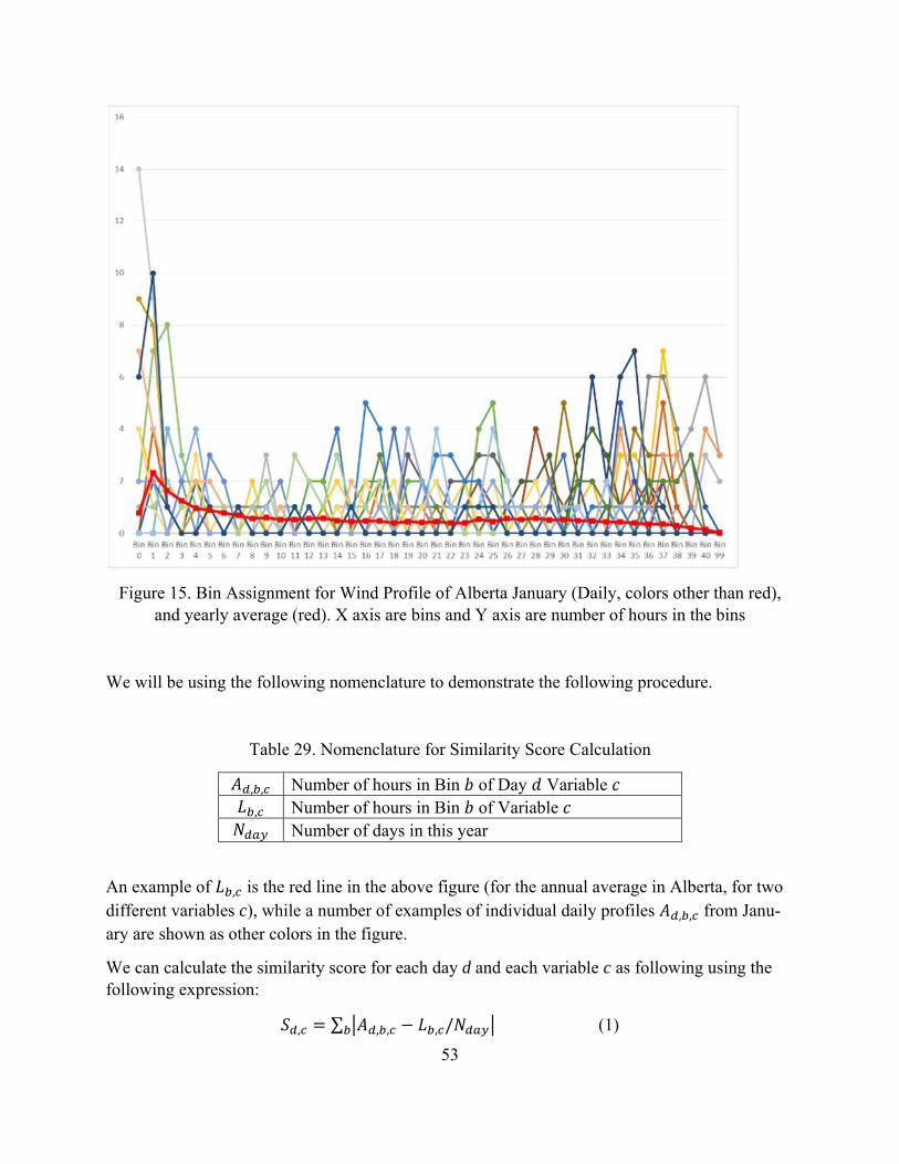
53

Figure 15. Bin Assignment for Wind Profile of Alberta January (Daily, colors other than red), and yearly average (red). X axis are bins and Y axis are number of hours in the bins

We will be using the following nomenclature to demonstrate the following procedure.

Table 29. Nomenclature for Similarity Score Calculation

, , Number of hours in Bin of Day Variable

, Number of hours in Bin of Variable Number of days in this year

An example of , is the red line in the above figure (for the annual average in Alberta, for two different variables c), while a number of examples of individual daily profiles , , from Janu-ary are shown as other colors in the figure.

We can calculate the similarity score for each day d and each variable c as following using the following expression:

, ∑ , , , / (1)

54

It is easy to see that a smaller score , indicates that for variable , day is relatively closer to the yearly average.

Step - 3. Clustering With the similarity score calculated, we immediately see that the similarity score matrix , is two-dimensional (i.e., for each day , , is a vector) and hence k-means clustering is readily used. We can use k-means clustering technique to cluster the days in to groups, based on how close the profiles are to the annual average. The user needs to specify the number of groups K that are desired.

Clustering the days are essential, since we not only want days that are very similar to the annual average, but also the days that are not, to retain the diversity of the days.

The clustering result with 4 is shown in the following table.

Table 30. Clustering Result with K=4

Cluster Days Total number ( ) 1 1-124, 290-365 200 2 125-174 50 3 175-251 77 4 252-289 38

Step - 4. Day Selection Finally, with the clusters identified, preparation for selecting days are complete. We have two approaches: random sampling plus result filtering and integer programing. No matter which ap-proach we use, the following properties are satisfied:

Certain objectives are optimized. These objectives can be one or more functions includ-ing minimizing the sum of first moment error across all profiles (the approach selected in this report), or a weighted sum of first moment error and second moment error or mini-mizing the final similarity score.

One day is selected from each cluster

For each cluster, the selected day will be assumed to repeat times, for which is the total number of days in cluster .

Approach 1 (optional): Random Selection plus result filtering This procedure is very simple:

Sample days from clusters (one day per cluster, thus days per sample) many times, and calculate the objective function.

Select the best or top samples that minimizing the objective function, e.g., sum of first moment error across all profiles

The random selection plus result filtering approach has the following features:

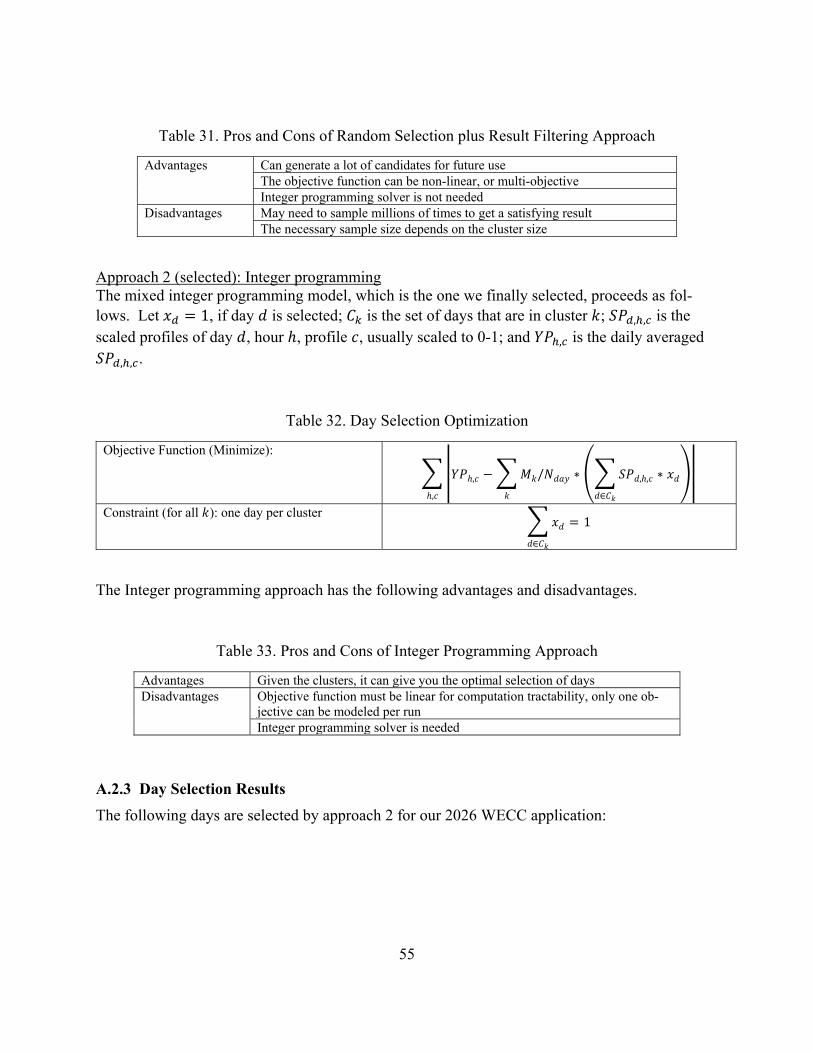
55

Table 31. Pros and Cons of Random Selection plus Result Filtering Approach

Advantages Can generate a lot of candidates for future useThe objective function can be non-linear, or multi-objective Integer programming solver is not needed

Disadvantages May need to sample millions of times to get a satisfying result The necessary sample size depends on the cluster size

Approach 2 (selected): Integer programming The mixed integer programming model, which is the one we finally selected, proceeds as fol-lows. Let 1, if day is selected; is the set of days that are in cluster ; , , is the scaled profiles of day , hour , profile , usually scaled to 0-1; and , is the daily averaged

, , .

Table 32. Day Selection Optimization

Objective Function (Minimize):

, / ∗ , , ∗

∈,

Constraint (for all ): one day per cluster

∈

1

The Integer programming approach has the following advantages and disadvantages.

Table 33. Pros and Cons of Integer Programming Approach

Advantages Given the clusters, it can give you the optimal selection of days Disadvantages Objective function must be linear for computation tractability, only one ob-

jective can be modeled per runInteger programming solver is needed

A.2.3 Day Selection Results

The following days are selected by approach 2 for our 2026 WECC application:

56

Table 34. Day Selection Result of Approach 2

Cluster 1 Cluster 2 Cluster 3 Cluster 4Day 31 Day 159 Day 200 Day 275

We can calculate the deviation between the first moments of profiles between the “pseudo-year” comprised of selected days and the original year 2026. The result is shown in Table 35: each cell shows how many profiles have the deviation specified in top row (left closed), e.g., 39 (sum of row 5, columns 5 and 6) out of 40 (row 5, total showed in most right column) load profiles have deviations within ±10%.

Table 35. The First Moment Deviation of the Year Comprised of Selected Days against the Orig-inal year

Deviation ≤-50% (-50%, -

25%] (-25%, -

10%] (-10%, 0] (0, 10%]

(10%, 25%]

(25%, 50%]

> 50% Total

Wind 7 7 13 3 9 26 26 7 98

Solar 0 0 18 25 18 13 4 0 78

Hydro 4 8 21 22 28 21 12 1 117

Load 0 0 0 19 20 1 0 0 40

Total 11 15 52 69 75 61 42 8 333

A.3 Features of the proposed Day Selection procedure

In this section, we highlight the features of this day selection procedure.

First, this procedure captures the statistics of the profiles (e.g., correlation, average etc.; for details, see previous sections of this Appendix)

Second, this procedure is only dependent on the original profiles of the WECC common case, and so can be used for both LTPT model and JHSMINE model.

Third, this is a click-and-run procedure (if the user chooses approach 1 in Step 4). All procedures are coded in R, and only minimal data massaging (such as determining which hour is in which day) is needed before running the procedure.

Finally, this procedure is highly customable, as we explain next.

A.4 Customization of Day Selection procedure

The customization of the proposed procedure is shown in the following table:

57

Table 36. Customization of Proposed Day Selection

Step CustomizationPreprocessing WECC users can add profiles or ignore profilesStep 1: Bin Assignment Bin assignment rule can be changed by WECC users Step 2: Similarity Score Calculation WECC user can specify which bin they think is more importantStep 3: Clustering Clustering method can be specified by WECC users, such as K-means

clustering, or Ward’s hierarchical clustering; number of clusters can be specified

Step 4: Day selection Different approaches can be selected; if using the random sampling method, different nonlinear objective function can be defined.

58

Appendix B. Generation and Storage Expansion Co-optimization with Consideration of Unit Commitment: Application to Storage-Transmission

Relations

Generation and Storage Expansion Co-optimization with Consideration of Unit Commitment

Qingyu Xu, Shenshen Li, and Benjamin F. Hobbs Department of Environmental Health and Engineering

The Johns Hopkins University Baltimore, U.S.A [email protected]

Abstract—A generation and storage expansion co-optimization model is formulated as an MILP. This expansion model is characterized by the inclusion of unit commitment modeling, such as the minimum run requirement, the ramp-rate limit, minimum up/down time and start-up/shut-down costs. Storage operation considering energy and power capacity limits and energy losses are also modeled. Storage and generation expansion is modeled as continuous variables, and an operating reserve requirement is included. The new formulation is tested in the IEEE RTS-24 test system, and the numerical results show the importance of considering unit commitment in generation and storage operation expansion modeling. Furthermore, the complementary and substitution relationships between intermittent resources and storage are quantified using the model; sometimes storage enhances the values of wind, but in other circumstances the reverse is true.

Keywords—Storage expansion; generation expansion; mixed integer programming; economics

I. NOMENCLATURE

A. Sets and subsets:

Buses, index Generators, index Generators located on bus

Storage facilities located on bus Storage facilities, index Transmission lines, index Operating periods, index

B. Parameters

, Load (MW) Maximum discharging time (duration) of (Hour)

Annualized generation capacity cost ($/MW-year) Annualized storage capacity cost ($/MW-year)

Period duration (Hour) A large number

Minimum down time (Hour) Minimum up time (Hour)

Minimum run (fraction of capacity) Minimum discharge and charge rate (fraction of

capacity)

, Minimum charge rate (fraction of storage capacity)

, Minimum discharge rate (fraction of storage capacity) Required up reserve (fraction of total demand) Ramping rate of (fraction of capacity)

S Line susceptance (MW) Unit start-up cost ($/MW capacity) Unit shut-down cost ($/MW capacity)

Thermal limit (MW) , Variable cost of generators ($/MWh)

, Variable cost of storages ($/MWh)

, Resource availability (fraction) Capacity potential of (MW)

Capacity potential of (MW) Charge and discharge efficiency of (fraction)

Φ , Bus-line incidence matrix element, 1 for “to” bus, -1 for “from” bus, 0 otherwise

C. Decision Variables

, Power flow in line l in period (MW)

, 1 if shuts down in period ; 0 otherwise

, State of charge of in period (MWh), non-negative

, Discharge of in period (MW), non-negative

, Charge of in period (MW), non-negative

, Ramp-down limit of in period t, non-negative

, Operating reserve offered by g in period , non-negative

, Operating reserve offered by in period , non-negative

, Ramp-up limit of in period t, non-negative

, Start-up cost of at ($), non-negative

, Shut-down cost of at ($), non-negative

, 1 if is on in period ; 0 otherwise

, 1 if starts up in period ; 0 otherwise

, 1 if is discharging at ; 0 otherwise

, 1 if is charging at ; 0 otherwise Installed capacity of (MW), non-negative

Installed capacity of (MW), non-negative

, Power output of in period (MW), non-negative

, Phase angle at bus in period

To Appear, Proceedings of the Probabilistic Methods Applied to Power Systems Conference, “Probabilistic Methods: Practical Approaches for Managing Risk and Uncertainty in the Electric Power Industry”, Boise Idaho, June 24, 28, 2018

II. INTRODUCTION

The rapidly falling cost of batteries [1] is making this technology a potential driver of the future mix of power generation technologies. Currently, power system operators and/or government have begun the process of adopting distributed storage in the grid. For example, Southern California Edison, a utility in California, USA, had contracted 400 MW of storage in its service area in 2017, which is double the total storage installed in the USA in 2015 [2].

One of the most important applications of energy storage is to help accommodate intermittent resources [3, 4]. Storage can absorb excess power generation from intermittent resources during times of low power prices and, on the other hand, discharge when prices are high. In this case, storage complements intermittent resources by decreasing curtailment and together providing more benefits.

However, storage can also benefit conventional thermal units, which often have limited flexibility: when a low net-load is observed, instead of shutting down, slow thermal plants can pay storage to absorb its excessive power. By doing this, storage benefits the system by avoiding expensive shut-downs and start-ups. Further, by making the operation of the conventional generation more economic, storage implicitly intensifies competition between conventional and intermittent resources, and thus can lower the benefits of the latter. In this circumstance, storage acts as an economic substitute for intermittent renewables.

Here we ask the following questions: How can we characterize the relationship between the intermittent resources and storage? In particular would more storage increase or decrease the economic value of renewables? I.e., do they complement or substitute for each other? Finally, how does more accurate modeling of thermal generation flexibility (i.e., unit commitment constraints and costs) affect estimates of the of the role and value of storage in a renewable-heavy system?

To answer these questions, a planning model is needed for generation and storage expansion problem that includes unit commitment.

Unit commitment (UC) modeling includes but is not limited to model ramping limits, minimum run limits and the costs of start-ups and shut-downs. Generation expansion planning with unit commitment has been modelled in [5-8]. In generation expansion planning (GEP), considering UC is difficult because UC usually involves a commitment variable multiplied by the capacity, which is a decision variable in GEP, and hence a non-linearity is introduced in the form of bilinear terms. However, this nonlinearity can be handled by modeling generation expansion using binary or integer variables [5-7]. Another approach, as in [8], is to linearize the unit commitment constraints so that a GEP with UC becomes a linear problem but with some loss of fidelity.

There is rich literature on storage expansion modeling, such as [4, 9, 10]. In [4], storage expansion problem is solved using particle swarm optimization, a metaheuristic optimization algorithm. In [9, 10], storage and transmission co-optimization is proposed, but generation capacities are treated as fixed.

The contribution of this work is two-fold. First, we propose a new formulation of the storage and generation expansion co-optimization with unit commitment, in which expansion variables are continuous. Second, we test this new formulation in the IEEE RTS-24 and address the following questions: Is unit commitment consideration important for modeling storage expansion? Do intermittent resources and storage substitute or complement each other?

III. GENERATION AND STORAGE EXPANSION CO-OPTIMIZATION

The problem is modeled as a static expansion planning problem. Thus, the objective is to minimize the annual system cost, which is composed of the variable cost of generation and storage, start-up and shut-down costs, and the annualized cost of capacity:

Variable costs are composed of fuel cost and variable O&M cost. Annualized cost of capacity includes the annualized cost of capacity and fixed O&M cost.

In the following subsection, each major set of constraints are discussed. Unit commitment constraints are similar to [6] [7] but differ in that 1) expansion variables are continuous and 2) ramp-rate, minimum run and storage operation are handled by disjunctive constraints. Wind generators are not subject to unit commitment constraints.

A. DC-OPF and Operating Reserve

Linearized Kirchhoff’s current and voltage laws are given in (2), for all bus and , and (3), for all lines and . Constraints (4) and (5) are transmission thermal limits and operating reserve requirements, respectively.

B. Start-up and Shut-down

For all conventional generators and operating periods :

Constraints (6) and (7) calculate the start-up and shut-down

costs of generation. For example, if the generator is started up in period , then the right-hand-side of (6) is the start-up cost; if

, , , ,

,

, ,

,

(1)

,

∈

,

∈

, , ,

∈

,

, Φ , ,

| , |

, , ,

(2)

(3)

(4)

(5)

, 1 ,

, 1 ,

, , , , 1

(6)

(7)

(8)

the generator is not started up, then constraint (6) is not binding, hence start-up cost will be minimized to zero. The start-up and shut-down logic is captured in constraint (8).

C. Ramp Rate Limits:

For all conventional generators and periods :

Constraints (9) and (10) are ramping-down and ramping-up

constraints. Ramping-up and down limits are imposed through disjunctive constraints (11-18). For example, if the generator is started up in period , then (11) and (12) will make sure that the ramp-rate limit is the minimum run level, and will ensure that the ramp-rate limits (13) and (14) are relaxed; on the other hand, if the generator is not started-up in period , then (11) and (12) are not binding, and (13) and (14) will make sure that the effective ramp-rate limit is the just the ramp-rate limit alone. The same goes for the ramp-down limits (15-18).

D. Minimum and Maximum Run, Minimum Up and Down Time

For all thermal generators and periods :

Constraint (19) is the minimum run constraint. Equations

(20-21) are the maximum run constraints: if a generator is started up, the maximum run is its capacity multiplied by the availability; if not, then the maximum run will be zero. Further, (22) and (23) are the minimum up and down constraints. For example, in (22), if in any time within the minimum up time range the generator had been started up, then the generator is not able to be turned off.

E. Storage Operation

For all storage units and periods :

Constraints (24-35) are storage operating constraints.

Constraint (24) makes sure that storage can only be in charge mode, discharge mode or idle. Constraints (25-30) are the discharge and charging limits of storage. For example, if storage is discharging, then (25) will force discharging to be higher than the minimum discharge rate; meanwhile, (26) will require that the discharge plus operating reserve to be no more than capacity. When storage is not discharging, (25) and (26) will be relaxed and (27) will force the discharge to zero. Specifically, since storage can provide operating reserves by curtailing charging, inequality (28) is making sure, in that situation, that the operating reserve lies between zero and the difference between the charging rate and the minimum charging. Constraints (31) is the state of charge limit. Constraint (32) is the operating reserve upper limit. Constraint (33) is the maximum potential of storage. Constraint (34) is the energy balance of storage. Constraint (35) enforces the operating reserve to be zero if the storage is idle. Please note that energy limits for reserve can be easily added, e.g., the state of charge at hour must be enough to support the current discharge plus the provided reserve. We drop them here since we assume that if operating reserves are drawn upon, that would only occur for a short duration (well below an hour) and hence the energy consumed is not significant compared to the length of the operating period.

IV. EXPERIMENT DESIGN

In this section, test cases are described that are designed to answer the research questions: 1) How important is it to consider unit commitment in a generation and storage expansion co-optimization model? And 2) Are intermittent resources and storages substitutes or complements for each other? First, the experiment environment is presented: a modified RTS-24 system [11] for generation and storage expansion. Second, how the experimental design addresses the above questions is explained and the test cases are summarized.

A. A Modified RTS-24 system

The RTS-24 system [11] is modified for generation and storage expansion as follows. The modifications include: 1) adding generation candidate sites (coal steam units, natural gas combustion turbines, natural gas combined cycle units, and wind), 2) adding storage candidate sites, 3) adding hourly wind

, , ,

, , , ,

, 1 ,

, 1 ,

, ,

, ,

, 1 ,

, 1 ,

, ,

, ,

(9) (10) (11) (12) (13) (14) (15) (16) (17) (18)

1 , ,

, , ,

, , ,

∑, ′

′

′ 1 ,

∑ , ′′

′ 1 1 ,

(19)

(20)

(21)

(22)

(23)

, , 1

1 , ,

1 , , ,

,

1 , , ,

1 , ,

,

,

, ,

,

, , , 1/ ,

, , ,

(24) (25) (26) (27) (28) (29) (30) (31) (32) (33) (34) (35)

availability profiles and 4) modifying the hourly loads. The transmission topology and the existing generators are unchanged in the RTS-24 system, with the exception that the operating costs (start-up, shut-down and variable costs) are tripled to set up an environment where wind is competitive. For the whole network, a 5% operating reserve requirement is also modeled, and can be met not only by the thermal plants but also by storage.

Generation and storage candidates: Conventional generation, namely coal, gas combustion turbine (CT) and combined cycle (CC) can be expanded at buses 3, 10 and 19, respectively, with no upper bound on the amount added. Wind turbines can be added on buses 3, 5, 7, 16, 21, 23 with a maximum potential of 200 MW on each bus. Storage candidates, assuming to be 8-hour Li-ion batteries, are located on bus 1, 3, 15 and 18 with a maximum potential of 200 MW each. Cost data can be found in TABLE I and Operation data in TABLE II. Capital cost and fixed O&M data is from [12] and the year is assumed to be 2026. An interest rate of 5% is assumed in the test cases.

TABLE I. CANDIDATE COST DATA IN THE MODIFIED RTS-24 SYSTEM

Tech Lifetime (years)

Fixed OM

($/kw-year)

Overnight. Cap. Cost

($/kW)

Annual. Cost of Cap. ($/kW-year)

Variable Cost

($/MWh)Bus

Wind 20 40 1718 177.8 0.00 3, 5, 7, 16, 21,

23Coal 40 35 3700 250.6 25.50 3CT 20 9 825 75.2 57.50 10CC 20 10 1300 114.3 39.65 19

Storage 15 30 3138 332.3 0.00 1, 3,

15, 18

TABLE II. CANDIDATE OPERATION DATA IN THE MODIFIED RTS-24 SYSTEM

Tech Minimum

Run (of capacity)

Ramp-Rate (% of

Capacity)

Startup Cost

($/MW)

MUT (Hours)

MDT (Hours)

Wind - - - - -Coal 51% 28.5% 61.26 24 24CT 41% 75% 24.32 1 1CC 51% 44.1% 59.68 6 8

Storage 10% Round-trip Efficiency = 92%, Duration = 8 Hours

Hourly wind availability and loads: Two 8760 hourly wind

availability curves of California (North and South) are obtained from the WECC TEPPC 2026 Common Case [13], and the 24-hour wind availability is calculated by averaging across 365 days and then renormalizing outputs to a 0-1 range, where 1 is the turbine capacity and 0 was the minimum output. The normalized 8760-hour load shape of balance area Turlock Irrigation District is selected, and the 24-hour load shape is calculated by averaging across 365 days. The maximum load of RTS-24 and the system-to-bus load distribution factors are unchanged. Wind farm candidates on bus 16, 21 and 23 (North) follow wind profile 1 and the others use wind profile 2 (South) Figure 1.

Figure 1. Assumed load (left axis, MW) and wind (right axis) profiles in the modified RTS-24 system

B. Test Cases

In order to answer the first question (Is unit commitment consideration important for modeling storage expansion?) the following test cases are designed (TABLE III). In principle, with capacity cost decreasing, more storage should be installed into the system (Cases 16, Cases 712, which include and exclude unit commitment, respectively). If the model without unit commitment starts to install the storages with a capacity cost lower than the model with unit commitment, this indicates that lack of unit commitment underestimates the benefit of storages to the system.

TABLE III. Test Cases to Analyze the Importance of Unit Commitment

Unit Commitment

Storage Cost of Capacity Compared to Baseline Level 100% 50% 40% 30% 10% 5%

Yes Case 1 Case 2 Case 3 Case 4 Case 5 Case

6

No Case 7 Case 8 Case 9 Case 10

Case 11

Case 12

We now summarize the cases that address the second

question: Do intermittent generation and storage substitute or complement each other? The definitions of substitute and complement effects in power system expansion are given first.

In power system expansion, planner optimize the portfolio of investment, e.g., generation, transmission and storage, in order to minimize the system cost, which is composed of investment cost and operation cost. If decreasing the cost of component A in the portfolio, e.g., less expensive wind, causes the planner to expand more of another component B, e.g., more investment in storage, then we say component A complements component B. This could happen when A and B can provide more benefits to the system together than the sum of their individual benefits if added individually. Similarly, if decreasing of capacity cost of component A causes a decreasing of component B in the planner’s expansion portfolio, then we say component A substitutes for B.

A total of 328 test cases are designed to test if the substitution and complement effects exist between wind and storages. In the

0

0.1

0.2

0.3

0.4

0.5

0.6

0.7

0.8

0.9

1

0

500

1000

1500

2000

2500

3000

3500

1 2 3 4 5 6 7 8 9 101112131415161718192021222324

load wind profile2 wind profile1

328 test cases, wind costs of capacity are varied from 50% to 120% of the baseline level in TABLE I (step size: 10%) and storage cost of capacity are ranging from 10% to 50% of the baseline level (step size: 1%). The optimal expansion plans of the test cases are compared to identify whether storage and wind investments exhibit a substitution or complement effect. All 328 test cases include the unit commitment formulation.

V. NUMERICAL RESULTS

In this section, the numerical results of the test cases are presented. All test cases are solved using CPLEX®12.6.3 to a Mixed Integer Programing (MIP) gap of 0.01%. Running time for each test case ranges from 1-3 seconds. The largest model had 4094 continuous variables, 1272 binary (unit commitment) variables, and 11030 constraints.

A. The Importance of Unit Commitnent to Storage Expansion

The storage expansion plan is shown in Table IV. Without unit commitment, model starts to invest in storage only when the capacity cost is at 5% of the original level (right column, last row). However, in test cases with unit commitment implemented, storage investments being to appear at much higher levels of annual capacity cost (at $99.7/kw-year, or about 30% of the original level) of the original level. These results imply that a planning model without unit commitment considerations will greatly underestimate the benefit that storage facility can provided to the system. However, the results also indicate that at current levels of annual capacity cost costs, (100%, or 332.3 $/kW-year) batteries are still not economic to the power system under our assumptions

TABLE IV. STORAGE EXPANSION PLANS IN TEST CASES 1-12

Storage Capacity Cost Level (% of baseline)

With Unit Commitment

Without Unit Commitment

100% 0 050% 0 040% 0 MW 030% 5.49 MW 010% 304.31 MW 05% 400.00 MW 276.55 MW

Because unit commitment constraints and costs

significantly affect the solution, we only use the unit commitment formulation to address the second question, next.

B. Substitutes and Complements: Impact of Wind Capacity Cost on Storage Expansion

In this subsection, the substitution and complementary relationships between storage and generation are explored. The results show that 1) both substitute and complement effects exist and 2) which one dominates depends on the cost level and the correlation between the intermittent resources and the load.

In Figure 2, the amount of storage added in different test cases are shown. Given a level of wind capacity cost, cheaper battery costs result in more battery investment, as might be expected. But the effect of cheaper wind on battery acquisition is ambiguous, as we now discuss.

We first identify the level of wind capacity cost at which at which 30 MW or more of storage starts to be acquired.

Interestingly, the levels of wind cost at which some storage becomes economic is between 80-90% of the baseline level if storage costs 30% or more its baseline cost. When wind capacity cost is below 80% or above 90%, storage needs to be much cheaper to enter the system in significant amounts. For example, when wind capacity cost is at 100% of its baseline, storage enters the system (amounting to115 MW) only when is cost at 19% of its baseline or less.

Figure 2. Total storage expansion (red axis, MW) in different test cases.

However, this trend (storage is more attractive when wind costs are intermediate) reverses when storage capacity costs became much lower. In the test cases where storage annual capacity cost costs are at 10-15% level, Figure 2 shows that the storage expansion is much lower (rather than higher) when wind capacity cost is in the 80-90% range, compared to when wind costs are lower or higher.

We make two remarks about these results. First, at a particular level of capacity costs, substitution or complement effects can both exist. For example, starting at the point where storage capacity cost is at 37% of the baseline and wind is at 90%, cheaper wind results in less storage expansion (substitute effect), while wind investment increases (discussed in the next section). On the other hand, starting from that point and then making wind more expensive also decreases storage investment (complement effect).

Second, the presence and strength of substitution or complement effects depends on the cost level of both resources. As noted earlier in this section, when storage capacity cost is very low, the effects can reverse compared to when storage costs are higher.

C. Substitute and Complement Effects: Impact of Storage Capacity Cost on Wind Expansion

As shown in the Section IV, candidate sites for new wind plants have two distinct wind production profiles, depending on their location. As shown in Figure 1, type 2 wind is more correlated with load. Figure 3 and Figure 4 show that the impact of decreasing storage capacity cost (from right to left) is different for two types of wind. For type 1 wind (Figure 3), the trends change when wind capacity cost decreases from 80% to

0.5 0.6 0.7 0.8 0.9 1 1.1 1.2

0

100

200

300

400

500

0.1

0.19

0.28

0.37

0.46

Sto

rage

Exp

ansi

on: (

MW

)

70% of the baseline level: in those cases, storage changes from substituting for wind (lower storage cost results less wind expansion) to complementing wind (lower storage cost increases wind investment). For type 2 wind, the trends are less straight forward: for a given wind capacity cost, both effects can be found, depending on the battery cost.

Figure 3. Capacity additions (MW) of wind following profile 1.

Figure 4. Capacity additions (MW) of wind following profile 2.

VI. DISCUSSION AND FUTURE WORK

Returning to the first research question: Is it necessary to consider unit commitment in a generation and storage expansion model? The numerical results emphasis the importance of unit commitment by showing that disregarding would result in much less storage in the system.

However, modeling unit commitment will usually introduce a lot more (binary) decision variables into the model and greatly slow down the model. This suggests that computationally more efficient models are needed when modeling storage and generation expansion for larger systems, especially if other complications are needed in the planning model, such as transmission expansion and stochastic programming.

The second question is: Are wind resources and storage substitutes or complements? The numerical results suggest that

both relationships can occur, depending on the level of wind and battery costs. Interestingly, this implies that wind resources do not necessarily make storage more attractive; indeed, the reverse can be true.

Future work should apply the formulation to larger networks, adding environmental policies such as renewable portfolio standards and carbon pricing.

ACKNOWLEDGMENT

This work is partially funded by the Western Electricity Coordinating Council. However, any opinions expressed or errors are the sole responsibility of the authors.

REFERENCES

[1] B. Nykvist and M. Nilsson, "Rapidly falling costs of battery packs for electric vehicles," Nature Climate Change, vol. 5, p. 329, 03/23/online 2015.

[2] SCE Battery Energy Storage Resources. Available: https://www.edison.com/home/innovation/energy-storage.html

[3] F. Steinke, P. Wolfrum, and C. Hoffmann, "Grid vs. storage in a 100% renewable Europe," Renewable Energy, vol. 50, pp. 826-832, 2013.

[4] R. Hemmati, H. Saboori, and M. A. Jirdehi, "Multistage generation expansion planning incorporating large scale energy storage systems and environmental pollution," Renewable Energy, vol. 97, pp. 636-645, 2016.

[5] B. S. Palmintier and M. D. Webster, "Impact of Operational Flexibility on Electricity Generation Planning With Renewable and Carbon Targets," IEEE Transactions on Sustainable Energy, vol. 7, no. 2, pp. 672-684, 2016.

[6] B. Hua, R. Baldick, and J. Wang, "Representing Operational Flexibility in Generation Expansion Planning Through Convex Relaxation of Unit Commitment," IEEE Transactions on Power Systems, 2017. [Online].

[7] A. Schwele, J. Kazempour, and P. Pinson, "Do unit commitment constraints affect generation expansion planning? A scalable stochastic model," Preprint submitted to Energy Economics, 2017.

[8] J. Ho, B. F. Hobbs, P. Donohoo-Vallett, Q. Xu, S. Kasina, S. W. Park, and Y. Ouyang, "Planning Transmission for Uncertainty: Applications and Lessons for the Western Interconnection," The Western Electricity Coordinating Council, 2016.

[9] Y. Dvorkin, R. Fernandez Blanco Carramolino, Y. Wang, B. Xu, D. Kirschen, H. Pandzic, J.-P. Watson, and C. A. Silva-Monroy, "Co-planning of Investments in Transmission and Merchant Energy Storage," IEEE Transactions on Power Systems, vol. 33, no. 1, pp. 245-256, 2018.

[10] T. Qiu, B. Xu, Y. Wang, Y. Dvorkin, and D. S. Kirschen, "Stochastic Multistage Coplanning of Transmission Expansion and Energy Storage," IEEE Transactions on Power Systems, vol. 32, no. 1, pp. 643-651, 2017.

[11] C. Ordoudis, P. Pinson, J. M. Morales González, and M. Zugno, "An Updated Version of the IEEE RTS 24-Bus System for Electricity Market and Power System Operation Studies," Technical University of Denmark (DTU), 2016.

[12] WECC and E3, "Review of Capital Costs for Generation Technologies," Salt Lake City, UT,2017, Available: https://www.wecc.biz/Reliability/E3_WECC_CapitalCosts_FINAL.pdf.

[13] WECC, "2026 Common Case Version 2.0," Salt Lake City, UT, 2017, Available: https://www.wecc.biz/Reliability/WECC%202026%20Common%20Case%20Version%202.0%20Release%20PackagePublic.zip.

0

100

200

300

400

500

600

700

0.1

0.12

0.14

0.16

0.18 0.2

0.22

0.24

0.26

0.28 0.3

0.32

0.34

0.36

0.38 0.4

0.42

0.44

0.46

0.48 0.5

0.5 0.6 0.7 0.80.9 1 1.1 1.2

X-axis: test-case cost/baseline cost

Series: wind test-case cost/baseline cost

0

100

200

300

400

500

600

700

0.1

0.12

0.14

0.16

0.18 0.

20.

220.

240.

260.

28 0.3

0.32

0.34

0.36

0.38 0.

40.

420.

440.

460.

48 0.5

0.5 0.6 0.7 0.80.9 1 1.1 1.2

X-axis: test-case cost/baseline cost

Series: wind test-case cost/baseline cost

Documents

Interactions of Energy Storage and Transmission … Final Project...Interactions of Energy Storage and Transmission Expansion Final Report May 2018 Qingyu Xu and Benjamin F. Hobbs