Embed Size (px)
Citation preview
Interaction-Induced Dynamics
in Ultracold Rydberg Gases –
Mechanical Effects and Coherent Processes
Thomas Amthor
Fakultat fur Mathematik und Physik
Albert-Ludwigs-Universitat Freiburg

Interaction-Induced Dynamics
in Ultracold Rydberg Gases –
Mechanical Effects and Coherent Processes
INAUGURAL-DISSERTATION
zur
Erlangung des Doktorgrades
der Fakultat fur Mathematik und Physik
der Albert-Ludwigs-Universitat
Freiburg im Breisgau
vorgelegt von
Dipl.-Phys. Thomas Amthor
aus Hanau
im Juli 2008

Dekan: Prof. Dr. Jorg Flum
Leiter der Arbeit: Prof. Dr. Matthias Weidemuller
Referent: Prof. Dr. Matthias Weidemuller
Koreferent:
Prufer: Prof. Dr. Andreas Buchleitner
Prof. Dr. Oskar von der Luhe
Tag der Verkundigung
des Prufungsergebnisses: 3. September 2008
III
Part of the work presented in this thesis has been published in the following articles:
• T. Amthor et al.
Controlling the pair distribution in an ultracold Rydberg gas
in prep.
• T. Amthor et al.
Probing Rabi oscillations using Ramsey interference in a three-level system
in prep.
• T. Amthor, J. Denskat, C. Giese, N. N. Bezuglov, A. Ekers, L. Cederbaum, M. Weidemuller
Autoionization of an ultracold Rydberg gas through resonant dipole coupling
in prep.
• T. Amthor, M. Reetz-Lamour, M. Weidemuller
Frozen Rydberg Gases
to appear in Cold Atoms and Molecules, Wiley-VCH (2008)
• T. Amthor, M. Reetz-Lamour, S. Westermann, J. Denskat, M. Weidemuller
Mechanical effect of van der Waals interactions observed in real time in an ultracold
Rydberg gas
Phys. Rev. Lett. 98, 023004 (2007)
• T. Amthor, M. Reetz-Lamour, C. Giese, M. Weidemuller
Modeling many-particle mechanical effects of an interacting Rydberg gas
Phys. Rev. A, 76, 054702 (2007)
• M. Reetz-Lamour, T. Amthor, J. Deiglmayr, M. Weidemuller
Rabi oscillations and excitation trapping in the coherent excitation of a mesoscopic
frozen Rydberg gas
Phys. Rev. Lett. 100, 253001 (2008)
• M. Reetz-Lamour, T. Amthor, S. Westermann, J. Denskat, M. Weidemuller
Modelling few-body phenomena in an ultracold Rydberg gas
Nucl. Phys. A 790, 728c (2007)
• O. Mulken, A. Blumen, T. Amthor, C. Giese, M. Reetz-Lamour, M. Weidemuller
Survival Probabilities in Coherent Exciton Transfer with Trapping
Phys. Rev. Lett. 99, 090601 (2007)
IV
• S. Westermann, T. Amthor, A.L. de Oliveira, J. Deiglmayr, M. Reetz-Lamour, M. Wei-
demuller
Dynamics of resonant energy transfer in a cold Rydberg gas
Eur. Phys. J. D 40, 37 (2006)
In addition, the author has contributed to the following publications:
• M. Reetz-Lamour, J. Deiglmayr, T. Amthor, M. Weidemuller
Rabi oscillations between ground and Rydberg states and van der Waals blockade in
a mesoscopic frozen Rydberg gas
New J. Phys. 10, 045026 (2008)
• A. H. Iavaronni, E. A. L. Henn, E. R. F. Ramos, J. A. Seman, T. Amthor, V. S. Bagnato
Evaporacao em armadilhas atomicas e as temperaturas mais baixas do Universo
Rev. Bras. Ens. Fıs. 29, 209 (2007)
• E. A. L. Henn, J. A. Seman, E. R. F. Ramos, A. H. Iavaronni, T. Amthor, V. S. Bagnato
Evaporation in atomic traps: A simple approach
Am. J. Phys. 75, 907 (2007)
• R. F. Shiozaki, E. A. L. Henn, K. M. F. Magalhaes, T. Amthor, V. S. Bagnato
Tunable electro-optical modulators based on a split-ring resonator
Rev. Sci. Inst. 78, 016103 (2007)
• J. Deiglmayr, M. Reetz-Lamour, T. Amthor, S. Westermann, A.L. de Oliveira, M. Wei-
demuller
Coherent excitation of Rydberg atoms in an ultracold gas
Opt. Comm. 264, 293 (2006)
• M. Reetz-Lamour, T. Amthor, J. Deiglmayr, S. Westermann, K. Singer, A.L. de Oliveira, L.G.
Marcassa, M. Weidemuller
Prospects of ultracold Rydberg gases for quantum information processing
Fortschr. Phys. 54, 776 (2006)
• K. Singer, M. Reetz-Lamour, T. Amthor, S. Folling, M. Tscherneck, M. Weidemuller
Spectroscopy of an ultracold Rydberg gas and signatures of Rydberg-Rydberg inter-
actions
J. Phys. B 38, S321 (2005)
V
• M. Weidemuller, M. Reetz-Lamour, T. Amthor, J. Deiglmayr, K. Singer, L.G. Marcassa
Interactions in an ultracold gas of Rydberg atoms
Laser Spectroscopy XVII, edited by E.A. Hinds, A. Ferguson, E. Riis (World Scientific,
New Jersey), 264-274 (2005)
• M. Weidemuller, K. Singer, M. Reetz-Lamour, T. Amthor, L.G. Marcassa
Ultralong-Range Interactions and Blockade of Excitation in a Cold Rydberg Gas
Atomic Physics XIX, edited by L.G. Marcassa, K. Helmerson and V.S. Bagnato, AIP Con-
ference Proceedings 770 (AIP, Melville), 157-163 (2004)
• K. Singer, M. Reetz-Lamour, T. Amthor, L. G. Marcassa, M. Weidemuller
Suppression of Excitation and Spectral Broadening Induced by Interactions in a Cold
Gas of Rydberg Atoms
Phys. Rev. Lett. 93, 163001 (2004)
VI
Abstract. In this thesis the dynamics of ultracold Rydberg gases under the influence of
long-range interactions is investigated, with regard to both the incoherent motion of the
atoms and coherent effects in the preparation and interaction of the gas. Due to their ex-
ceptional properties, these highly excited atoms have a great potential for applications in
many different areas, while requiring an increasing degree of understanding and control
of the complex many-body dynamics in the gas. One important aspect is the interaction-
induced motion, which can lead to collisions and decoherence. As shown here, this mo-
tion is one of the main processes triggering autoionization and ultracold plasma formation,
and can be controlled by detuned laser excitation. Ionizing collisions are exploited as a
sensitive probe to reveal variations in the Rydberg pair distribution. Another requirement
for controlled manipulation of the system, the coherent excitation of the Rydberg sample,
is demonstrated in terms of Rabi oscillations and Ramsey interference. Finally, the co-
herence of many-body interactions is investigated in different spatial arrangements. The
possibility to control interactions and to realize exciton traps make Rydberg atoms an ideal
model system for resonant energy transfer processes. In this regard an implementation of
structured arrangements of Rydberg atoms is proposed.
Zusammenfassung. Diese Arbeit untersucht die durch langreichweitige Wechselwirkung
in ultrakalten Rydberg-Gasen induzierte Dynamik, im Hinblick sowohl auf inkoharente
Bewegung der Atome als auch auf koharente Effekte in der Prapration und Wechselwir-
kung des Gases. Wegen ihrer außergewohnlichen Eigenschaften haben die hochangereg-
ten Atome ein großes Anwendungspotential in verschiedenen Bereichen, wobei in zuneh-
mendem Maße Verstandnis und Kontrolle der komplexen Vielteilchendynamik im Gas er-
forderlich ist. Ein wichtiger Aspekt ist dabei die wechselwirkungsinduzierte Bewegung,
die zu Kollisionen und Dekoharenz fuhren kann. Wie hier gezeigt, ist dies einer der grund-
legenden Prozesse, die zur Autoionisation und Bildung ultrakalter Plasmen fuhren, der
aber durch verstimmte Anregung kontrolliert werden kann. Stoßionisation kann als emp-
findliche Sonde fur Variationen in der Rydberg-Paarverteilung genutzt werden. Eine wei-
tere Voraussetzung fur kontrollierte Manipulation des Systems, die koharente Rydberg-
Anregung, wird in Form von Rabi-Oszillationen und Ramsey-Interferenz demonstriert.
Schließlich wird die Koharenz von Vielteilchen-Wechselwirkungen in verschiedenen
raumlichen Anordnungen untersucht. Die Moglichkeit der Kontrolle der Wechselwirkun-
gen und der Realisierung von Exzitonen-Fallen machen Rydbergatome zu einem idea-
len Modellsystem fur Energietransfer-Prozesse. Hierzu wird eine Implementierung einer
strukturierter Anordnung von Rydbergatomen vorgeschlagen.
VII
”Vi far inte rum med flera namn i vara huvuden,”
skreko ungarna. ”Vi far inte rum med flera namn i
vara huvuden.” — ”Ju mera, som kommer in i ett
huvud, desto battre rum blir det,” svarade forargasen
och fortsatte att ropa ut de markvardiga namnen pa
samma satt.
– Selma Lagerlof,
Nils Holgerssons underbara resa genom Sverige

VIII
Contents
1 Introduction 1
2 Rydberg atoms 7
2.1 Rydberg states of alkali atoms . . . . . . . . . . . . . . . . . . . . . . . 9
2.2 Wavefunctions and dipole matrix elements . . . . . . . . . . . . . . . . . 11
2.3 Stark structure . . . . . . . . . . . . . . . . . . . . . . . . . . . . . . . . 16
2.4 Experimental setup . . . . . . . . . . . . . . . . . . . . . . . . . . . . . 18
3 Interactions in a Rydberg gas 27
3.1 Long-range interactions . . . . . . . . . . . . . . . . . . . . . . . . . . . 27
3.2 Pair distribution functions . . . . . . . . . . . . . . . . . . . . . . . . . . 34
3.3 Influence of surrounding atoms . . . . . . . . . . . . . . . . . . . . . . . 37
3.4 Ionization processes . . . . . . . . . . . . . . . . . . . . . . . . . . . . . 39
4 Mechanical effects of Rydberg interactions 55
4.1 Monte-Carlo excitation model . . . . . . . . . . . . . . . . . . . . . . . 56
4.2 Dynamics of attractive Rydberg systems . . . . . . . . . . . . . . . . . . 58
4.3 Dynamics of repulsive Rydberg systems . . . . . . . . . . . . . . . . . . 66
4.4 Dynamics on a Forster resonance . . . . . . . . . . . . . . . . . . . . . . 74
4.5 Shaping the pair distribution . . . . . . . . . . . . . . . . . . . . . . . . 77
4.6 Using Autler-Townes splitting for excitation control . . . . . . . . . . . . 80
5 Coherence in Rydberg gases 93
5.1 Rabi oscillations . . . . . . . . . . . . . . . . . . . . . . . . . . . . . . . 94
5.2 Ramsey interference . . . . . . . . . . . . . . . . . . . . . . . . . . . . 97
5.3 Resonant energy transfer in an unordered gas . . . . . . . . . . . . . . . 105
IX
X CONTENTS
5.4 Energy transport in one-dimensional chains . . . . . . . . . . . . . . . . 116
5.5 Experimental realization of energy transport . . . . . . . . . . . . . . . . 119
6 Conclusion and outlook 129
A Three-level systems and Optical Bloch Equations 135
B LCoS beam shaping 139
C Ultrastable cavity lock 143
D Electronic circuits 151
Acknowledgements 159
Bibliography 162
Chapter 1
Introduction
Rydberg atoms, highly excited atomic states with intriguing properties, have been subject
to experimental investigations since many decades. While in the early years of Rydberg
physics only hot vapor and atomic beams were available, today’s techniques of laser cool-
ing and trapping allow insight into the world of ultracold, frozen Rydberg gases, where
the thermal energies are much smaller than the typical interaction energies. The dynamics
of such a system is completely determined by long-range interactions.
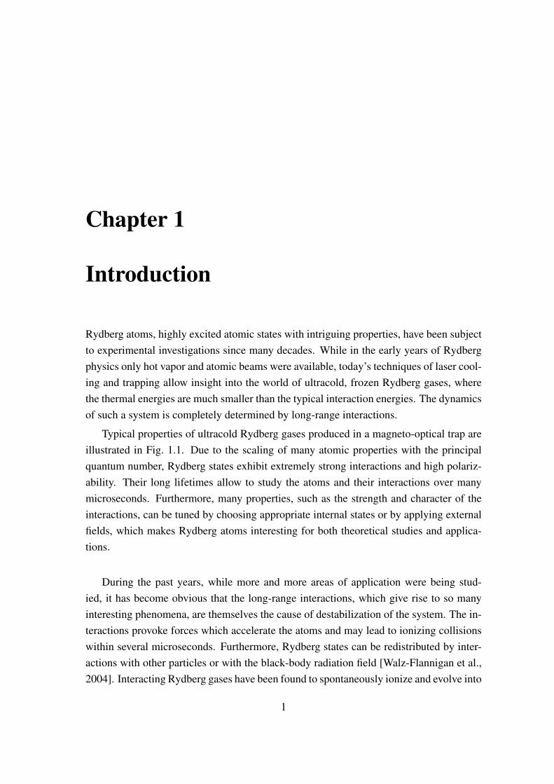
Typical properties of ultracold Rydberg gases produced in a magneto-optical trap are
illustrated in Fig. 1.1. Due to the scaling of many atomic properties with the principal
quantum number, Rydberg states exhibit extremely strong interactions and high polariz-
ability. Their long lifetimes allow to study the atoms and their interactions over many
microseconds. Furthermore, many properties, such as the strength and character of the
interactions, can be tuned by choosing appropriate internal states or by applying external
fields, which makes Rydberg atoms interesting for both theoretical studies and applica-
tions.
During the past years, while more and more areas of application were being stud-
ied, it has become obvious that the long-range interactions, which give rise to so many
interesting phenomena, are themselves the cause of destabilization of the system. The in-
teractions provoke forces which accelerate the atoms and may lead to ionizing collisions
within several microseconds. Furthermore, Rydberg states can be redistributed by inter-
actions with other particles or with the black-body radiation field [Walz-Flannigan et al.,
2004]. Interacting Rydberg gases have been found to spontaneously ionize and evolve into
1
2 CHAPTER 1. INTRODUCTION
Figure 1.1: Properties of ultracold Rydberg gases produced in a magneto-optical trap. The
strong long-range interactions are observable over the typical distances of several microns.
Due to their low thermal velocities and long lifetimes, the interaction-induced dynamics of
the system can be investigated over many microseconds.
a plasma1 [Robinson et al., 2000, Li et al., 2004, Gallagher et al., 2003], a phenomenon
which before had only been known from hot dense gases [Vitrant et al., 1982]. It is there-
fore of great importance to understand the dynamics of interacting Rydberg gases and
to find ways of controlling and stabilizing the system. Even though the mechanisms of
autoionization in ultracold gases are still not understood in all detail [Tanner et al., 2008],
interaction-induced collisions have been suspected to be one of the main processes con-
tributing to the initial ionization of Rydberg gases. Collisions on dipole-dipole interaction
potentials have been evoked using microwave spectroscopy [Li et al., 2005]. Collisions
induced by van der Waals interactions, the dominant type of interactions in a gas of atoms
prepared in a specific Rydberg state, are indeed identified to be the main contribution to
autoionization of the gas [Amthor et al., 2007a, Amthor et al., 2007b], as shown in the
framework of this thesis. It is further shown that the dynamics of the ionization process
can be controlled by variations in the pair distribution of the Rydberg atoms induced by
different excitation schemes. Despite being undesirable for most applications, collisional
ionization is also found to be a sensitive probe for interaction potentials and pair distribu-
tions.
1The physics of ultracold plasmas is an interesting field of research of its own, especially because of the
possible strong coupling [Killian et al., 2007], which has led to a number of studies about ultracold plasma
formation and evolution , e.g. [Kulin et al., 2000, Robicheaux and Hanson, 2002, Pohl et al., 2003].
3
One of the major fields of application for ultracold Rydberg gases has been opened
by theoretical proposals of how to exploit Rydberg atoms and their strong long-range in-
teractions for the purpose of quantum information processing [Jaksch et al., 2000, Lukin
et al., 2001]. The proposed gate operations rely on the concept of the dipole block-
ade, an interaction-induced inhibition of excitation, which should make it possible to
prepare mesoscopic atom samples sharing a single Rydberg excitation. The first obser-
vations of excitation suppression by van der Waals interaction (including the work in our
group) [Tong et al., 2004,Singer et al., 2004] were followed by investigations of suppres-
sion induced by dipole-dipole interaction [Vogt et al., 2006,Vogt et al., 2007]. The block-
ade manifests itself in a change of counting statistics [Cubel Liebisch et al., 2005] and has
recently been observed in systems with only two interacting atoms [Urban et al., 2008].
When the density of the atoms is increased significantly, interaction effects become dra-
matic. Excitation suppression and collective excitation have recently been investigated in
very dense samples and even in Bose-Einstein condensates [Heidemann et al., 2007, Hei-
demann et al., 2008, Raitzsch et al., 2008]. In this high-density regime, the excitation
suppression is found to be described by a universal power law [Weimer et al., 2008].
Meanwhile alternative schemes for quantum gate operations have been proposed, even
without the requirement of a dipole blockade [Cozzini et al., 2006] and without substantial
population of the Rydberg state [Brion et al., 2007b]. A recent idea is to encode quantum
information in multilevel quantum systems [Brion et al., 2007a, Saffman and Mølmer,
2008]. All of these applications require that the Rydberg excitation process can be con-
trolled to a high degree in order to maximize excitation efficiency and to create well-
known superpositions of states. Rapid adiabatic passage turns out to be robust scheme
to transfer population to Rydberg states [Cubel et al., 2005, Deiglmayr et al., 2006] and
even to prepare maximally entangled states in the presence of interactions [Møller et al.,
2008]. The coherent coupling of the atom to the light field further allows one to study
electromagnetically induced transparency (EIT), which has been used for non-destructive
optical probing of Rydberg states [Mohapatra et al., 2007]. Rydberg gases also exhibit
a very strong electro-optic effect [Mohapatra et al., 2008]. Rabi oscillations between
ground and Rydberg state, one prerequisite for Rydberg gate operations, have been ob-
served in few-body samples [Johnson et al., 2008], and, by our group, in mesoscopic
clouds [Reetz-Lamour et al., 2008a, Reetz-Lamour et al., 2008b]. As an interesting ex-
tension, the coherence in the excitation of Rydberg states can be observed via Ramsey
4 CHAPTER 1. INTRODUCTION
interference in a three-level system, as described in this thesis.
Another intriguing phenomenon which occurs in Rydberg gases is the resonant energy
transfer process, induced by resonant dipole coupling of the atomic levels. One reason for
the broad interest in this subject is the possibility to control the coupling strength by sim-
ply tuning an electric field. In earlier hot vapor experiments, energy transfer could be de-
scribed in terms of binary collisions [Stoneman et al., 1987]. In a frozen gas, however, the
process has be be considered as a many-particle effect [Anderson et al., 1998,Mourachko
et al., 1998], which allows to study many-body physics in a controllable way [Anderson
et al., 2002,Akulin et al., 1999]. Energy transfer in Rydberg gases is related to similar pro-
cesses in otherwise very different systems. Resonant energy transfer has first been studied
in photosynthesis, where energy is transported radiationless among molecules [Forster,
1948]. The extremely efficient energy transport in biological systems has again become
an area of active research [Ritz and Schulten, 2001]. Similar energy transfer processes are
relevant for organic electronics and organic solar cells, where energy is transported by dye
molecules [Gregg, 2003,Schlosser and Lochbrunner, 2006]. While in all of these transport
systems, energy transfer takes place among molecules, Rydberg systems allow to study
these processes with discrete atomic levels. Due to the ability to tune the interaction
strength and to deliberately induce coupling to continua or other sources of decoherence,
structured Rydberg atom arrangements may in future serve as a model system for tailored
energy transfer. Together with the group of Prof. Blumen, we have proposed a possible
experimental implementation of such a structured arrangement of Rydberg atoms to in-
vestigate energy transport under the presence of exciton traps [Mulken et al., 2007]. Our
experimental investigations of energy transfer dynamics in a many-body system [Wester-
mann et al., 2006] and observations of excitation trapping [Reetz-Lamour et al., 2008a],
both being essential ingredients for the proposed scheme, are also presented in the context
of this thesis.
The wide range of phenomena connected with ultracold Rydberg atoms demonstrate
that these systems are valuable tools in many different areas. Further investigations and
applications in all of these areas require a detailed understanding of the coherent and
incoherent dynamic processes present in ultracold interacting Rydberg gases, in order to
prepare and manipulate the system in a controlled way. The investigations presented in
this thesis, which cover both the mechanical motion induced by long-range interactions
5
and the coherence in the excitation and interaction of Rydberg atoms, constitute one step
in this direction. The work is structured as follows:
Chapter 2 gives an introduction of the physics of alkali Rydberg atoms, and introduces
the experimental setup used to prepare and detect Rydberg atoms in ultracold gases. The
calculation of Rydberg wavefunctions and dipole matrix elements is also reviewed.
Interactions among Rydberg atoms are discussed in Chapter 3. After an introduction
of long-range dipole interactions some properties of many-particle systems are described.
The interaction-induced ionization processes found in ultracold Rydberg gases are ad-
dressed in detail, as they are of particular importance for the experimental work presented
in the following chapters.
Chapter 4 covers the experimental observation of interaction-induced motion and the
dynamics of interaction-induced ionization in an initially frozen Rydberg gas under the
influence of attractive and repulsive interaction. A Monte Carlo model of the many-
particle system allows to extract information about the interaction potentials and the pair
distribution in the gas. The distribution of distances in the atom cloud can be controlled
to some degree by different configurations of detuned narrow-bandwidth excitation.
Coherent effects are discussed in Chapter 5. Rabi oscillations between ground and
Rydberg state are observed in a mesoscopic ensemble and the Autler-Townes splitting
of an intermediate state is used to create Ramsey interference patterns. The coherence
of resonant energy transfer in Rydberg gases is described with a few-body model and
compared to experimental observations. This chapter also presents a proposal for the
implementation of a regular arrangement of atoms with the possibility to insert excitation
traps, and provides experimental evidence for excitation trapping in internal states.
Finally, Chapter 6 gives a summary of the results and presents perspectives for fu-
ture experiments. Some technical improvements and electronic circuits which have been
developed in the course of this work are presented in the appendix.

6 CHAPTER 1. INTRODUCTION
Chapter 2
Rydberg atoms
In 1885 Johann Balmer realized that the wavelength of spectral lines of hydrogen could
be expressed with a simple formula [Balmer, 1885],
λ=m2
1
m21 −m2
2
h , (2.1)
where m1 and m2 are integer numbers (m2 = 2 for the Balmer series) and h is a constant.
Johannes Rydberg reformulated these findings in terms of wavenumbers (corresponding
to energy), which led to the expression of the binding energies of hydrogen
Ebind = −Ry
n2. (2.2)
Ry is called the Rydberg constant, its value for hydrogen is 13.6 eV. With the development
of the Bohr’s model of the atom, n was understood as the principal quantum number
[Bohr, 1913]. Bohr found the Rydberg constant to be connected to other fundamental
constants,
Ry =Z2e4me
2(4πε0h)2, (2.3)
with Z the charge of the atomic nucleus in units of e, e the electron charge, me the electron
mass, ε0 the vacuum permittivity, and h Planck’s constant.
The simple expression in Eq. (2.2) allows to calculate energy levels of very high prin-
cipal quantum numbers n, the Rydberg states. Even some fundamental scaling laws of
different atomic properties with the principal quantum number can easily be derived from
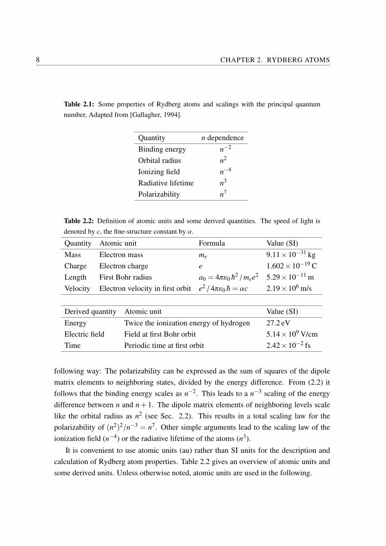
Bohr’s picture. Some of the most important quantities and their scaling exponents are
listed in Table 2.1. As an example, the scaling of the polarizability can be deduced in the
7
8 CHAPTER 2. RYDBERG ATOMS
Table 2.1: Some properties of Rydberg atoms and scalings with the principal quantum
number, Adapted from [Gallagher, 1994].
Quantity n dependence
Binding energy n−2
Orbital radius n2
Ionizing field n−4
Radiative lifetime n3
Polarizability n7
Table 2.2: Definition of atomic units and some derived quantities. The speed of light is
denoted by c, the fine-structure constant by α.
Quantity Atomic unit Formula Value (SI)
Mass Electron mass me 9.11×10⁻³¹ kg
Charge Electron charge e 1.602×10⁻¹⁹ C
Length First Bohr radius a0 = 4πε0 h2 /mee
2 5.29×10⁻¹¹ m
Velocity Electron velocity in first orbit e2 /4πε0 h = αc 2.19×10⁶ m/s
Derived quantity Atomic unit Value (SI)
Energy Twice the ionization energy of hydrogen 27.2 eV
Electric field Field at first Bohr orbit 5.14×10⁹ V/cm
Time Periodic time at first orbit 2.42×10⁻² fs
following way: The polarizability can be expressed as the sum of squares of the dipole
matrix elements to neighboring states, divided by the energy difference. From (2.2) it
follows that the binding energy scales as n−2. This leads to a n−3 scaling of the energy
difference between n and n+ 1. The dipole matrix elements of neighboring levels scale
like the orbital radius as n2 (see Sec. 2.2). This results in a total scaling law for the
polarizability of (n2)2/n−3 = n7. Other simple arguments lead to the scaling law of the
ionization field (n−4) or the radiative lifetime of the atoms (n3).
It is convenient to use atomic units (au) rather than SI units for the description and
calculation of Rydberg atom properties. Table 2.2 gives an overview of atomic units and
some derived units. Unless otherwise noted, atomic units are used in the following.
2.1. RYDBERG STATES OF ALKALI ATOMS 9
2.1 Rydberg states of alkali atoms
Electronically excited alkali atoms have much in common with the simple hydrogen atom.
Their single valence electron can be excited to a high-lying state, while the remaining
electrons stay close to the core and shield the core charge, so that the effective core charge
becomes Z = 1. Only when the angular momentum of the valence electron is small (ℓ≤ 3)
can it penetrate this extended core and the binding energies for these levels are increased.
This is accounted for by introducing the quantum defect δn,ℓ, j which depends on the quan-
tum numbers n, ℓ, and j:
En,ℓ, j = Ei−Ry
(n−δn,ℓ, j)2. (2.4)
The quantum defect can be calculated with high precision using the extended Rydberg-
Ritz formula
δn,ℓ, j = δ0 +δ2
(n−δ0)2+
δ4
(n−δ0)4+
δ6
(n−δ0)6+
δ8
(n−δ0)8. (2.5)
The constants δi are specific for each element. The corresponding values for rubidium are
given in Table 2.3. States with ℓ > 4 do not penetrate the core region considerably and
their quantum defect is zero. These degenerate states are therefore called hydrogen-like
states. In the following sections, the symbol n∗ will be used for the effective principal
quantum number including the quantum defect,
n∗ = n−δn,ℓ, j . (2.6)
With the Rydberg constant for rubidium RyRb = 109736.605 cm−1 and its ionization en-
ergy ERbi = 33690.798(2) cm−1, measured from the center of gravity of the hyperfine
split ground state [Lorenzen and Niemax, 1983], the laser frequency for the excitation of
a specific Rydberg state can be calculated very accurately.
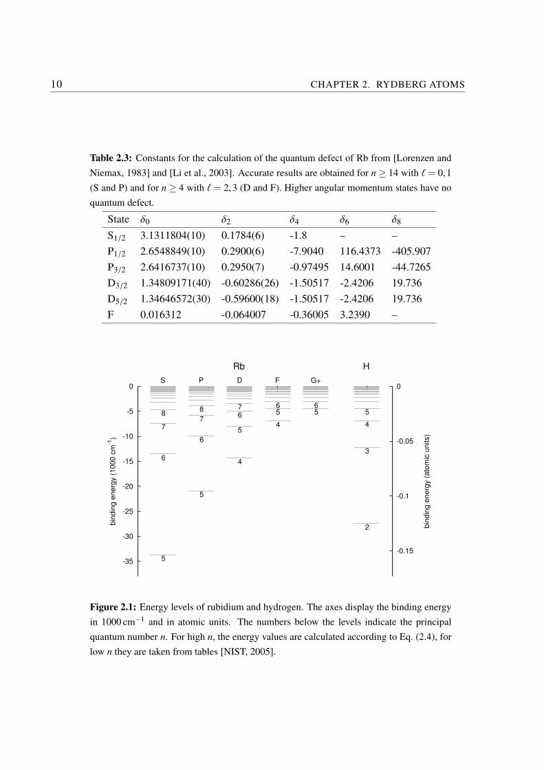
Fig. 2.1 illustrates the relative position of the energy levels of rubidium and hydrogen.
In rubidium, the states with low angular momentum ℓ ≤ 3 are shifted with respect to the
hydrogen levels due to the quantum defect. States with ℓ > 3 (marked G+) are degenerate
(hydrogen-like). The scale is given in cm−1 and in atomic units. The state n = 1 of
hydrogen (not shown) has the binding energy 1/2 in atomic units.
10 CHAPTER 2. RYDBERG ATOMS
Table 2.3: Constants for the calculation of the quantum defect of Rb from [Lorenzen and
Niemax, 1983] and [Li et al., 2003]. Accurate results are obtained for n≥ 14 with ℓ = 0,1
(S and P) and for n≥ 4 with ℓ = 2,3 (D and F). Higher angular momentum states have no
quantum defect.
State δ0 δ2 δ4 δ6 δ8
S1/2 3.1311804(10) 0.1784(6) -1.8 – –
P1/2 2.6548849(10) 0.2900(6) -7.9040 116.4373 -405.907
P3/2 2.6416737(10) 0.2950(7) -0.97495 14.6001 -44.7265
D3/2 1.34809171(40) -0.60286(26) -1.50517 -2.4206 19.736
D5/2 1.34646572(30) -0.59600(18) -1.50517 -2.4206 19.736
F 0.016312 -0.064007 -0.36005 3.2390 –
-35
-30
-25
-20
-15
-10
-5
0
-0.15
-0.1
-0.05
0
bin
din
g e
nerg
y (
1000 c
m-1
)
bin
din
g e
nerg
y (
ato
mic
units)
S P D F G+
Rb H
5
6
7
8
5
6
7
8
4
5
67
4
56
56
2
3
4
5
Figure 2.1: Energy levels of rubidium and hydrogen. The axes display the binding energy
in 1000 cm−1 and in atomic units. The numbers below the levels indicate the principal
quantum number n. For high n, the energy values are calculated according to Eq. (2.4), for
low n they are taken from tables [NIST, 2005].
2.2. WAVEFUNCTIONS AND DIPOLE MATRIX ELEMENTS 11
2.2 Wavefunctions and dipole matrix elements
Similar to the hydrogen problem, the wavefunctions of the alkali electrons in a stationary
picture can be expressed as the energy eigenstates of the Hamilton operator for a one-
electron atom,(
−∆2
2µ− Z
r
)
ψ= Eψ . (2.7)
Here ψ is the wavefunction of the electron and E is the corresponding energy. The reduced
mass of the atom (core plus electron) is denoted µ, and r is the distance of the electron
from the core. The wavefunction ψ can be separated in a radial and a spherical term,
ψ=1
rUnℓ(r)Yℓm(θ,ϕ) (2.8)
where the spherical part is expressed in terms of the spherical harmonics Yℓm(θ,ϕ) [Saku-
rai, 1994,Cohen-Tannoudji et al., 1999]. Inserting this separated form of ψ into Eq. (2.7),
an expression for radial part of the wavefunctions alone is obtained:
(
− 1
2µ
d2
dr2− Z
r+ℓ(ℓ+1)
2µr2
)
Unℓ(r) = EUnℓ(r) (2.9)
As discussed before, the energy E is given by the principal quantum number n and the
quantum defect δnℓ j,
E = − 1
2(n−δnℓ j)2(2.10)
so that Unℓ j(r) can be calculated. Eq. (2.9) is solved by numerical integration from a large
value of r inwards using the Numerov algorithm [Blatt, 1967, Numerov, 1924, Numerov,
1927]. The spacing between the many nodes of a Rydberg wavefunction becomes smaller
and smaller for decreasing r. This suggests the the use of scaled coordinates for the
numerical integration [Bhatti et al., 1981].
For low principal quantum numbers n of alkali atoms, the core potential Z/r assumed
in Eq. (2.7) is not a good description, because the core penetration of the electron is no
longer negligible. In this case, the simple Coulomb potential must be replaced by an
ℓ-dependent model potential which is better adapted to the alkali configuration [Aymar,
1978, Marinescu et al., 1994],
Vℓ(r) = −Zℓ(r)
r− αc
2r4
(
1− e−(r/rc)6)
, (2.11)
12 CHAPTER 2. RYDBERG ATOMS
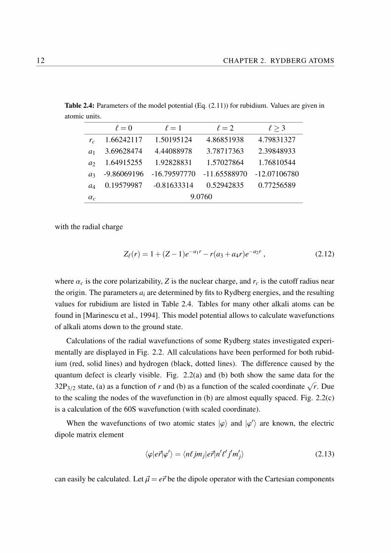
Table 2.4: Parameters of the model potential (Eq. (2.11)) for rubidium. Values are given in
atomic units.
ℓ = 0 ℓ = 1 ℓ = 2 ℓ ≥ 3
rc 1.66242117 1.50195124 4.86851938 4.79831327
a1 3.69628474 4.44088978 3.78717363 2.39848933
a2 1.64915255 1.92828831 1.57027864 1.76810544
a3 -9.86069196 -16.79597770 -11.65588970 -12.07106780
a4 0.19579987 -0.81633314 0.52942835 0.77256589
αc 9.0760
with the radial charge
Zℓ(r) = 1+(Z−1)e−a1r− r(a3 +a4r)e−a2r , (2.12)
where αc is the core polarizability, Z is the nuclear charge, and rc is the cutoff radius near
the origin. The parameters ai are determined by fits to Rydberg energies, and the resulting
values for rubidium are listed in Table 2.4. Tables for many other alkali atoms can be
found in [Marinescu et al., 1994]. This model potential allows to calculate wavefunctions
of alkali atoms down to the ground state.
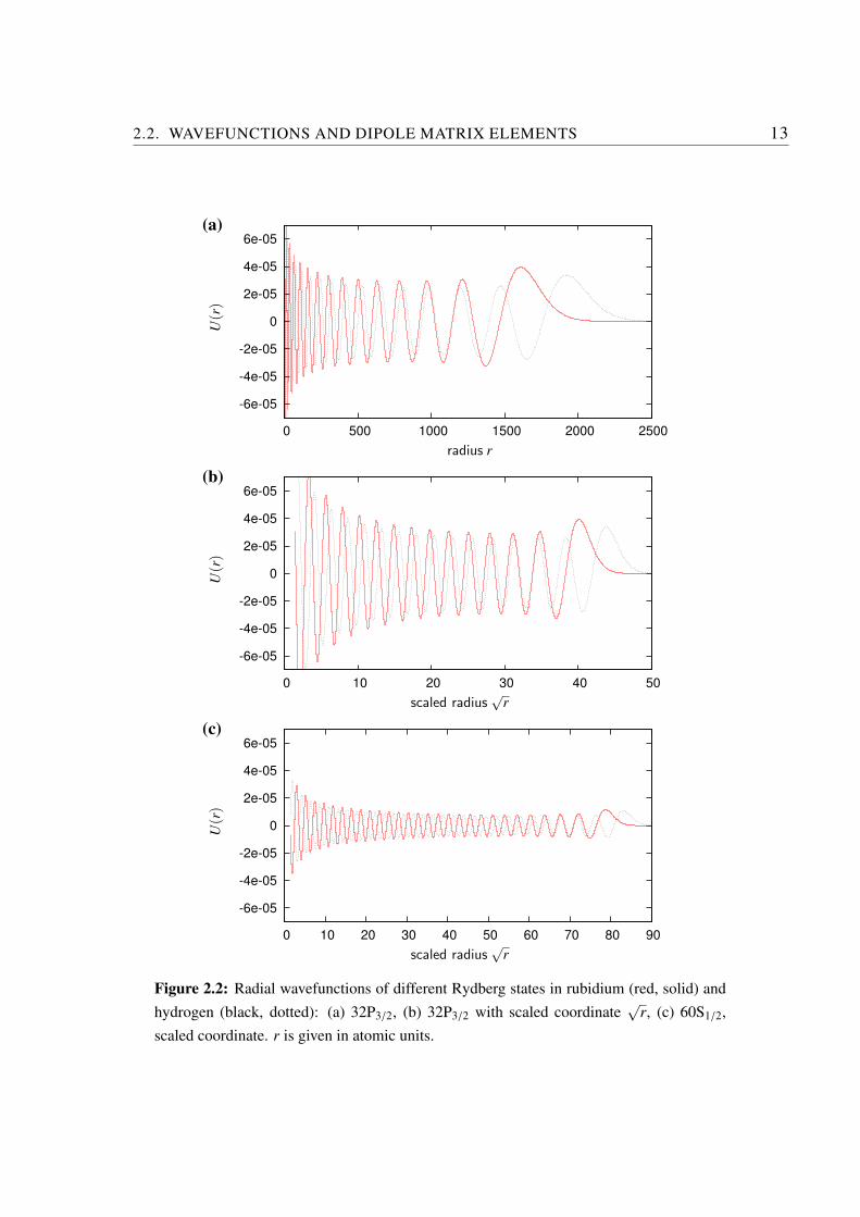
Calculations of the radial wavefunctions of some Rydberg states investigated experi-
mentally are displayed in Fig. 2.2. All calculations have been performed for both rubid-
ium (red, solid lines) and hydrogen (black, dotted lines). The difference caused by the
quantum defect is clearly visible. Fig. 2.2(a) and (b) both show the same data for the
32P3/2 state, (a) as a function of r and (b) as a function of the scaled coordinate√r. Due
to the scaling the nodes of the wavefunction in (b) are almost equally spaced. Fig. 2.2(c)
is a calculation of the 60S wavefunction (with scaled coordinate).
When the wavefunctions of two atomic states |ϕ〉 and |ϕ′〉 are known, the electric
dipole matrix element
〈ϕ|e~r|ϕ′〉 = 〈nℓ jm j|e~r|n′ℓ′ j′m′j〉 (2.13)
can easily be calculated. Let ~µ= e~r be the dipole operator with the Cartesian components
2.2. WAVEFUNCTIONS AND DIPOLE MATRIX ELEMENTS 13
(a)
-6e-05
-4e-05
-2e-05
0
2e-05
4e-05
6e-05
0 500 1000 1500 2000 2500
U(r
)
radius r
(b)
-6e-05
-4e-05
-2e-05
0
2e-05
4e-05
6e-05
0 10 20 30 40 50
U(r
)
scaled radius√r
(c)
-6e-05
-4e-05
-2e-05
0
2e-05
4e-05
6e-05
0 10 20 30 40 50 60 70 80 90
U(r
)
scaled radius√r
Figure 2.2: Radial wavefunctions of different Rydberg states in rubidium (red, solid) and
hydrogen (black, dotted): (a) 32P3/2, (b) 32P3/2 with scaled coordinate√r, (c) 60S1/2,
scaled coordinate. r is given in atomic units.
14 CHAPTER 2. RYDBERG ATOMS
0.01
0.1
40 50 60 70 80 90
dip
ole
matr
ix e
lem
ent
principal quantum number n
1000
10000
dip
ole
matr
ix e
lem
ent
|nS〉 ↔ |nP〉
|5P〉 ↔ |nS〉
|5P〉 ↔ |nD〉
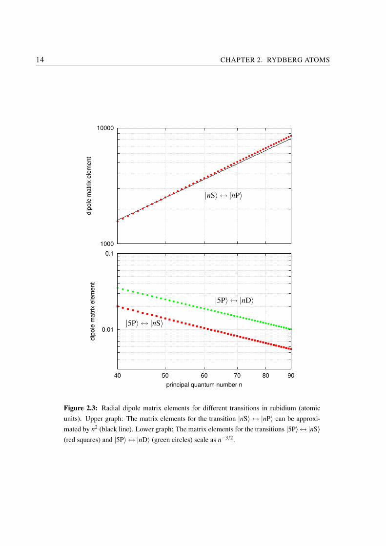
Figure 2.3: Radial dipole matrix elements for different transitions in rubidium (atomic
units). Upper graph: The matrix elements for the transition |nS〉 ↔ |nP〉 can be approxi-
mated by n2 (black line). Lower graph: The matrix elements for the transitions |5P〉↔ |nS〉(red squares) and |5P〉 ↔ |nD〉 (green circles) scale as n−3/2.
2.2. WAVEFUNCTIONS AND DIPOLE MATRIX ELEMENTS 15
µx, µy, µz. The operator can be expressed in a spherical basis with the components
µ−1 = 1/√
2(µx − iµy) (2.14)
µ0 = µz (2.15)
µ+1 = 1/√
2(µx + iµy) (2.16)
which can be rewritten in terms of the spherical harmonics as
µq = er
√
4π
3Y1,q , q = 0,±1 . (2.17)
Using the separation ansatz (2.8), the matrix elements of the dipole operator component
µq can be expressed as
〈nℓ jm j|µq|n′ℓ′ j′m′j〉 = ∑
ms,m′s
⟨
1
rUn,ℓ, j
∣
∣
∣
∣
er
∣
∣
∣
∣
1
rUn′,ℓ′, j′
⟩
×⟨
j,m j
∣
∣
∣
∣
ℓ,mℓ−ms,1
2,ms
⟩
×√
4π
3
⟨
Yℓ,m j−mS
∣
∣
∣Y1,q
∣
∣
∣Yℓ′,m′j−m′
s
⟩
×⟨
1
2,ms
∣
∣
∣
∣
1
2,m′
s
⟩
×⟨
j′,m′j
∣
∣
∣
∣
ℓ′,m′ℓ−m′
s,1
2,m′
s
⟩
.
(2.18)
The first factor in the sum depends only on the radial part of the wavefunction. It is
called the radial dipole matrix element and can be calculated numerically with the radial
wavefunctions obtained above. The other factors are the spherical contributions to the
matrix element, and do not depend on the radial wave function. They contain Clebsch-
Gordan coefficients from which selection rules and transition strengths can be derived.
The total spherical matrix element can be calculated by evaluating the expressions in
Eq. (2.18). It is also described in textbooks on quantum mechanics, see for example
[Sakurai, 1994].
Some calculated absolute values of radial dipole matrix elements for rubidium are
plotted in Fig. 2.3 as a function of the principal quantum number n. The matrix elements
for the transition |nS〉 ↔ |nP〉 are shown in the upper plot. Their value in atomic units
is very well approximated by n2, as indicated by the black line. In the lower graph the
16 CHAPTER 2. RYDBERG ATOMS
-0.04
-0.02
0
0.02
0.04
0.06
0 0.02 0.04 0.06 0.08 0.1 0.12 0.14
fre
qu
en
cy (
GH
z)
electric field (V/cm)
87D5/2
87D3/2
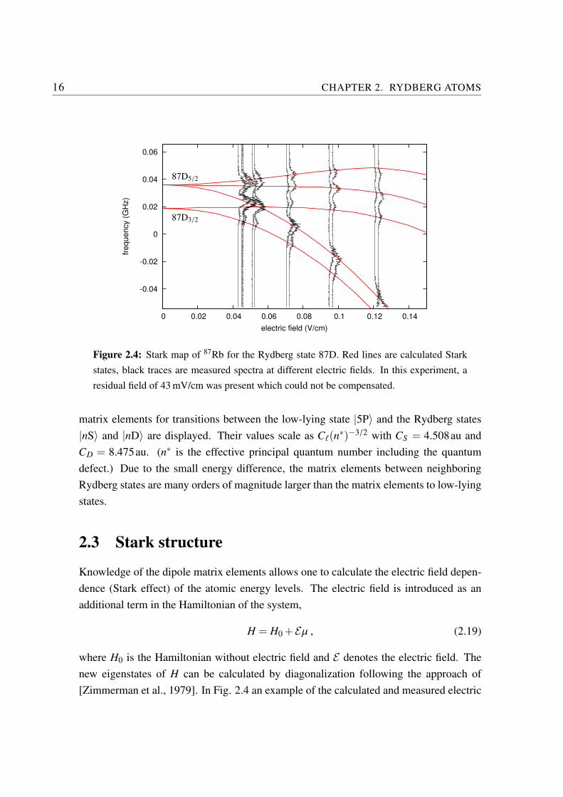
Figure 2.4: Stark map of 87Rb for the Rydberg state 87D. Red lines are calculated Stark
states, black traces are measured spectra at different electric fields. In this experiment, a
residual field of 43 mV/cm was present which could not be compensated.
matrix elements for transitions between the low-lying state |5P〉 and the Rydberg states
|nS〉 and |nD〉 are displayed. Their values scale as Cℓ(n∗)−3/2 with CS = 4.508au and
CD = 8.475au. (n∗ is the effective principal quantum number including the quantum
defect.) Due to the small energy difference, the matrix elements between neighboring
Rydberg states are many orders of magnitude larger than the matrix elements to low-lying
states.
2.3 Stark structure
Knowledge of the dipole matrix elements allows one to calculate the electric field depen-
dence (Stark effect) of the atomic energy levels. The electric field is introduced as an
additional term in the Hamiltonian of the system,
H = H0 +Eµ , (2.19)
where H0 is the Hamiltonian without electric field and E denotes the electric field. The
new eigenstates of H can be calculated by diagonalization following the approach of
[Zimmerman et al., 1979]. In Fig. 2.4 an example of the calculated and measured electric
2.3. STARK STRUCTURE 17
field dependence (Stark map) around the 87D state of rubidium is shown. The graph
visualizes how sensitive Rydberg states are on external electric fields. Large splittings
of the m j components and line shifts in the GHz range are observed already at electric
fields as small as a few V/cm. The electric field dependence of the Rydberg states will
be of importance for many of the experiments described here and calculated Stark maps
of atomic states and pair states will reappear several times throughout this thesis (see for
example Secs. 4.4, 5.4).
Due to their sensitivity on external fields, Rydberg atoms can also be used as a probe
to determine and compensate electric stray fields in the experiment. The electric field in
the region of the MOT can be divided in two components, E‖ and E⊥, parallel and perpen-
dicular to the symmetry axis of the setup, respectively. The electric field component E‖can be canceled by the field EFP generated by the field plates around the MOT. The total
electric field is then given by
E =√
(E⊥ +EFP)2 +E‖2 . (2.20)
The best possible field compensation thus always leaves a residual field E‖. E‖ and E⊥can be determined by plotting the scans for different settings of EFP on the calculated
Stark map and varying E‖ and E⊥ as parameters to find the best possible overlap. For
the experimental configuration used in Fig. 2.4, the field components are estimated to be
E‖ ≈ 255mV/cm and E⊥ ≈ 43mV/cm. (The residual fields in the setup are mainly caused
by high-voltage supply cables for the ion detector.)
If the electric field is increased above a critical value Ecrit, the atom is field-ionized.
The critical electric field can be estimated as [Gallagher, 1994, Gallagher et al., 1976,
Ducas et al., 1975, Stebbings et al., 1975]
Ecrit =1
16(n∗)−4 a.u. (2.21)
≈ 3.21×10⁸ (n∗)−4 V/cm . (2.22)
Here n∗ is the effective principal quantum number including the quantum defect. This
expression is useful to obtain an approximate value of the ionizing field. The exact process
of field ionization of an ultracold Rydberg gas is complex, as avoided crossings may also
be passed adiabatically [Han and Gallagher, 2008].
18 CHAPTER 2. RYDBERG ATOMS
2.4 Experimental setup
This section provides an overview of the experimental setup for the production and the
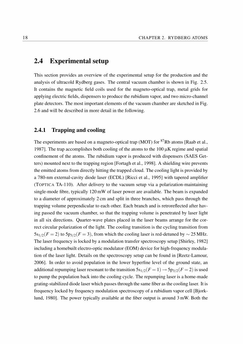
analysis of ultracold Rydberg gases. The central vacuum chamber is shown in Fig. 2.5.
It contains the magnetic field coils used for the magneto-optical trap, metal grids for
applying electric fields, dispensers to produce the rubidium vapor, and two micro-channel
plate detectors. The most important elements of the vacuum chamber are sketched in Fig.
2.6 and will be described in more detail in the following.
2.4.1 Trapping and cooling
The experiments are based on a magneto-optical trap (MOT) for 87Rb atoms [Raab et al.,
1987]. The trap accomplishes both cooling of the atoms to the 100 µK regime and spatial
confinement of the atoms. The rubidium vapor is produced with dispensers (SAES Get-
ters) mounted next to the trapping region [Fortagh et al., 1998]. A shielding wire prevents
the emitted atoms from directly hitting the trapped cloud. The cooling light is provided by
a 780-nm external-cavity diode laser (ECDL) [Ricci et al., 1995] with tapered amplifier
(TOPTICA TA-110). After delivery to the vacuum setup via a polarization-maintaining
single-mode fibre, typically 120 mW of laser power are available. The beam is expanded
to a diameter of approximately 2 cm and split in three branches, which pass through the
trapping volume perpendicular to each other. Each branch and is retroreflected after hav-
ing passed the vacuum chamber, so that the trapping volume is penetrated by laser light
in all six directions. Quarter-wave plates placed in the laser beams arrange for the cor-
rect circular polarization of the light. The cooling transition is the cycling transition from
5s1/2(F = 2) to 5p3/2(F = 3), from which the cooling laser is red-detuned by ∼ 25 MHz.
The laser frequency is locked by a modulation transfer spectroscopy setup [Shirley, 1982]
including a homebuilt electro-optic modulator (EOM) device for high-frequency modula-
tion of the laser light. Details on the spectroscopy setup can be found in [Reetz-Lamour,
2006]. In order to avoid population in the lower hyperfine level of the ground state, an
additional repumping laser resonant to the transition 5s1/2(F = 1)→ 5p3/2(F = 2) is used
to pump the population back into the cooling cycle. The repumping laser is a home-made
grating-stabilized diode laser which passes through the same fiber as the cooling laser. It is
frequency locked by frequency modulation spectroscopy of a rubidium vapor cell [Bjork-
lund, 1980]. The power typically available at the fiber output is around 3 mW. Both the
2.4. EXPERIMENTAL SETUP 19
(a)
(b)
6
5
3
3
47
8
1
1
2
2
2
6
Figure 2.5: Central part of the vacuum chamber. (a) Rendered CAD image, (b) Photograph
of the assembly before installation of the windows. (1) Vacuum chamber, (2) MOT coils,
(3) Ioffe coil (not used in the experiments), (4) rubidium dispensers, (5) position of the
atom cloud, (6) MCP detector, (7) MCP shielding grid, (8) wire meshes encasing trapping
region.
20 CHAPTER 2. RYDBERG ATOMS
MOT lasers
780 nm
excitation
480 nm
MCP
detector
field plates
vacuum
chamber
excitation
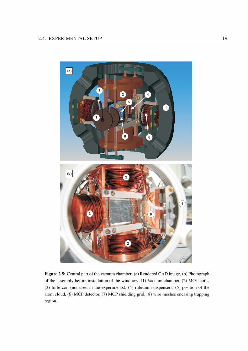
780 nm
Figure 2.6: Schematic view of the vacuum chamber with lasers and detection setup. The
excitation lasers at 780 nm and 480 nm are counter-propagating. Field plates (wire meshes)
and MCP detector are also shown.
cooling and the repumping laser can be switched on an off by acousto-optic modulators
(AOM). The relevant atomic energy levels for cooling and trapping of 87Rb are depicted
in Fig. 2.7.
The magnetic field for spatial confinement is provided by coils in anti-Helmholtz con-
figuration which are mounted inside the vacuum (see Fig. 2.5). A field gradient of ap-
proximately 20 G/cm is present in the trap region. A detailed description of the design
is given in [Tscherneck, 2002]. Three pairs of Helmholtz coils around the chamber are
used to compensate external magnetic fields [Deiglmayr, 2006]. A very precise method
of field compensation is based on the mechanical Hanle effect [Kaiser et al., 1991] which
has been successfully implemented in this setup [Reetz-Lamour, 2006]. The magnetic
field used for trapping can be switched on and off with a MOSFET (BUK456) to allow
for a field-free environment during Rydberg excitation.
The density, size, and temperature of the trapped atom cloud can be determined from
fluorescence imaging [Folling, 2003]. For this purpose the setup is equipped with a sensi-
tive CCD camera (THETA SYSTEMS SIS1-P18M) and imaging optics. Typically around
107 atoms are trapped at peak densities on the order of 1010 cm−3 and temperatures of
∼100 µK. The fluorescence of the MOT is also permanently recorded with a photo diode.
2.4. EXPERIMENTAL SETUP 21
~780nm
Rydberg states
~480 nm
6.83 GHz
72.2 MHz
156.9 MHz
266.7 MHz
excit
ati
on
repum
per
cooling +
tra
ppin
g
excit
ati
on
n = ∞
n≈ 30nℓ
F = 0
F = 1
F = 1
F = 2
F = 2
F = 3
5s1/2
5p3/2
δE
δM
Figure 2.7: Level scheme of the D2 line of 87Rb and the transition to Rydberg states. The
different laser transitions used for cooling and trapping, as well as for Rydberg excitation
are indicated. δM is the detuning of the cooling laser, δE is the (variable) detuning of the
excitation lasers from the intermediate level.
22 CHAPTER 2. RYDBERG ATOMS
2.4.2 Excitation of Rydberg states
The Rydberg excitation scheme involves two photons (see Fig. 2.7). The first photon
may be resonant with the transition 5s1/2(F = 2) → 5p3/2(F = 3), or be detuned by
δE , depending on the specific requirements of the experiment. It can be provided by
different lasers available in the setup. Unless otherwise noted, the experiments presented
in this thesis made use of a tapered laser chip (TOPTICA DLX-110) with a separate EOM
modulation branch and modulation transfer lock, delivered to the vacuum setup through
a separate optical fiber.
The second photon at 480 nm is provided by a frequency-doubled amplified diode
laser (TOPTICA TA-SHG). The master laser, running at 960 nm, can be tuned over a wide
range, so that Rydberg levels from n = 30 up to the ionization continuum are accessible.
The typical output power of the second-harmonic generation (SHG) cavity is 100 mW.
In contrast to the 780-nm lasers, this excitation laser cannot be referenced to any atomic
transition in a rubidium vapor cell. In order to stabilize the frequency against both short-
term fluctuations and long-term drifts, the laser is locked to an ultrastable reference cavity.
A detailed description of the cavity lock can be found in appendix C. The two excitation
lasers are counter-propagating (See Fig. 2.6). In most of the experiments discussed here,
the 480-nm laser is sent through a polarization-maintaining single-mode fiber for mode
cleaning and reproducible alignment, and is then focused with a lens of 100 mm focal
length to a waist of 37 µm in the MOT. This results in a cigar-shaped excitation volume
containing roughly 50 000 atoms.
The frequency of the 480-nm laser must be known with at least 1 GHz precision to dis-
tinguish Rydberg states with high principal quantum number and to set the laser frequency
to exactly the desired Rydberg state. The required frequency can easily be calculated ac-
cording to Eq. (2.2), taking the quantum defect into account. A homebuilt wavemeter is
used to measure the laser frequency. The apparatus consists of a Michelson interferometer
with moving retroreflectors. The number of interference fringes observed while moving
the reflectors is compared to a HeNe reference laser traveling the same way.
The excitation lasers are switched on for a short time, typically 100 ns to 1 µs. The
laser at 780 ns is switched with an AOM, while for the laser at 480 nm two switching meth-
ods are available. Either another AOM can be used, or a Pockels cell (LASERMETRICS
5046SC). The Pockels cell has the advantage of very fast switching times without mixing
additional frequencies into the excitation laser. For experiments requiring a time delay
2.4. EXPERIMENTAL SETUP 23
after the excitation, the Pockels cell may not be suited because of ringing effects which
can cause leaking of laser light > 1µs after the pulse. Laser pulse shapes produced by
the different switching elements and recorded by a fast photodiode are can be found in
Fig. 4.20 (blue laser switched by AOM) and Fig. 5.7 (blue laser switched by Pockels cell).
The density of Rydberg atoms can be varied in a controlled way by changing the
density of atoms in the 5p3/2 state. This is accomplished by turning off the repumping
laser for a well-defined time, while leaving the trapping laser on. In this way atoms are
pumped down into the dark 5s1/2(F = 1) hyperfine ground state and the population of
5p3/2 decreases. The time constant of this decrease can be determined by monitoring the
fluorescence of the atoms. This technique is for example applied for the measurements of
the energy transfer dynamics in Sec. 5.3.
2.4.3 Detection techniques
Rydberg states are detected by field ionization. A voltage high enough to field-ionize the
Rydberg state is applied to the nickel wire meshes (BUCKBEE MEARS MN-4) encasing
the trapped atom cloud. The meshes have a distance of 15 mm. All high voltages used
in the setup are provided by ISEG NHQ206L-s voltage supplies and switched with fast
high voltage switches (BEHLKE HTS 31-GSM). If state-selective detection is required
or if Rydberg atoms and previously produced ions should be discriminated, the electric
field is not switched on directly, but ramped up by an additional low pass filter (time
constant 10µs) between the switch and the field grids. Depending on the Rydberg state,
the required ionization fields vary drastically, reaching from only a few V/cm at high
quantum numbers (n > 80) to several hundred V/cm for n∼ 35.
The ionization field also accelerates ions towards the microchannel plate detector
(MCP). When hitting the detector, the ions release an electron avalanche which even-
tually leads to a short current flow through a resistor connected to the detector output.
The corresponding voltage pulse at this resistor is amplified, while the high voltage dc
part of the signal is blocked by a capacitor.
The setup offers two possibilities to process the ion signal: Either the peaks are inte-
grated by gated integrators, or single ion pulses are counted by a fast discriminator and
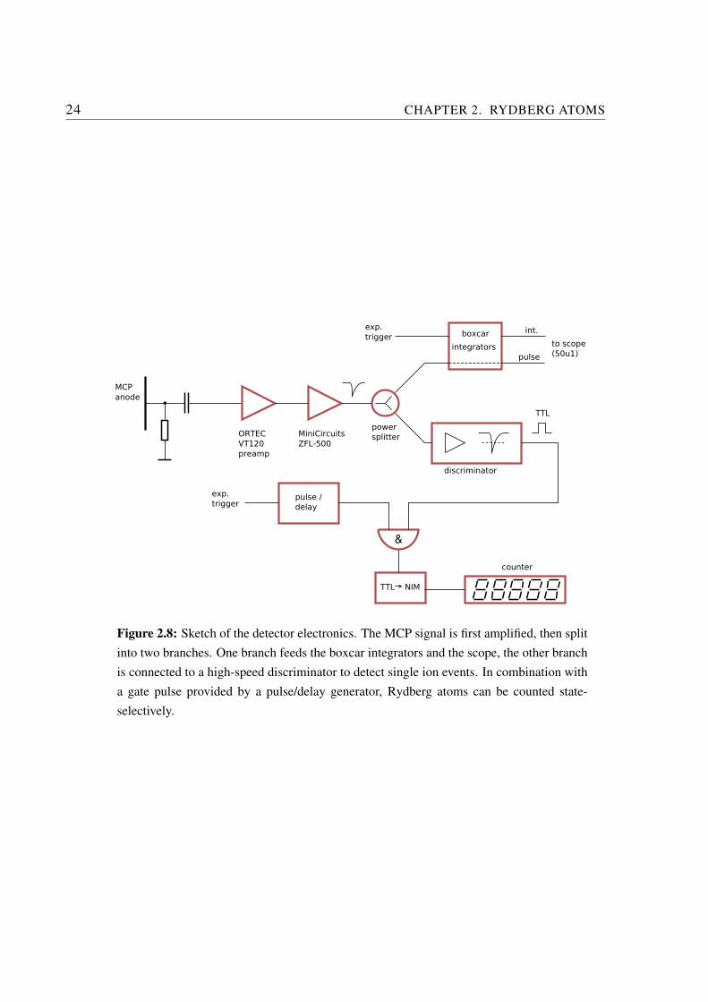
counter circuit. A simplified sketch of the electronics is depicted in Fig. 2.8. The MCP
output is fed into a fast preamplifier (ORTEC VT120) and then into a second amplifier
stage (MINICIRCUITS ZFL-500). A power splitter is used to split the signal line in two
24 CHAPTER 2. RYDBERG ATOMS
MCP
anode
ORTEC
VT120
preamp
MiniCircuits
ZFL−500
power
splitter
discriminator
TTL
pulse /
delay
TTL NIM
counter
exp.
trigger
exp.
trigger boxcar
integrators to scope
(50u1)
&
int.
pulse
Figure 2.8: Sketch of the detector electronics. The MCP signal is first amplified, then split
into two branches. One branch feeds the boxcar integrators and the scope, the other branch
is connected to a high-speed discriminator to detect single ion events. In combination with
a gate pulse provided by a pulse/delay generator, Rydberg atoms can be counted state-
selectively.
2.4. EXPERIMENTAL SETUP 25
0
500
1000
1500
2000
2500
3000
3500
4000
4500
-452 -451 -450 -449 -448 -447 -446 -445
de
tecto
r sig
na
l (a
rb.
u.)
energy relative to continuum (GHz)
88P3/2
88P5/2
87D 89S1/2
86h
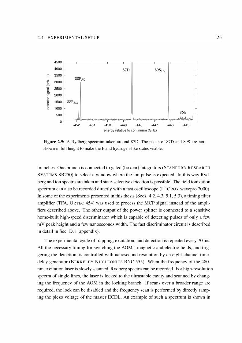
Figure 2.9: A Rydberg spectrum taken around 87D. The peaks of 87D and 89S are not
shown in full height to make the P and hydrogen-like states visible.
branches. One branch is connected to gated (boxcar) integrators (STANFORD RESEARCH
SYSTEMS SR250) to select a window where the ion pulse is expected. In this way Ryd-
berg and ion spectra are taken and state-selective detection is possible. The field ionization
spectrum can also be recorded directly with a fast oscilloscope (LECROY wavepro 7000).
In some of the experiments presented in this thesis (Secs. 4.2, 4.3, 5.1, 5.3), a timing filter
amplifier (TFA, ORTEC 454) was used to process the MCP signal instead of the ampli-
fiers described above. The other output of the power splitter is connected to a sensitive
home-built high-speed discriminator which is capable of detecting pulses of only a few
mV peak height and a few nanoseconds width. The fast discriminator circuit is described
in detail in Sec. D.1 (appendix).
The experimental cycle of trapping, excitation, and detection is repeated every 70 ms.
All the necessary timing for switching the AOMs, magnetic and electric fields, and trig-
gering the detection, is controlled with nanosecond resolution by an eight-channel time-
delay generator (BERKELEY NUCLEONICS BNC 555). When the frequency of the 480-
nm excitation laser is slowly scanned, Rydberg spectra can be recorded. For high-resolution
spectra of single lines, the laser is locked to the ultrastable cavity and scanned by chang-
ing the frequency of the AOM in the locking branch. If scans over a broader range are
required, the lock can be disabled and the frequency scan is performed by directly ramp-
ing the piezo voltage of the master ECDL. An example of such a spectrum is shown in
26 CHAPTER 2. RYDBERG ATOMS
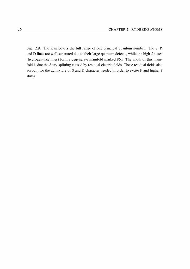
Fig. 2.9. The scan covers the full range of one principal quantum number. The S, P,
and D lines are well separated due to their large quantum defects, while the high-ℓ states
(hydrogen-like lines) form a degenerate manifold marked 86h. The width of this mani-
fold is due the Stark splitting caused by residual electric fields. These residual fields also
account for the admixture of S and D character needed in order to excite P and higher ℓ
states.
Chapter 3
Interactions in a Rydberg gas
Rydberg atoms are strongly polarizable and therefore react very sensitively on their en-
vironment, on other atoms in their vicinity, and on external fields. This Chapter gives an
overview of interaction effects in a gas of Rydberg atoms and their implications on the
dynamics of such a system. Sec. 3.1 is an introduction to binary dipole interactions and
discusses one important consequence of these interactions, the excitation blockade. In
the next two sections some essential properties and of many-body systems are addressed:
Sec. 3.2 introduces pair distribution functions, and in Sec. 3.3 the influence of surround-
ing atoms on a nearest-neighbor pair is described in general terms. Finally, in Sec. 3.4
different interaction-induced ionization processes are discussed in detail. This involves
interaction-induced motion, binary and many-particle effects – concepts which determine
the dynamics of the gas and which are of particular importance for the experiments pre-
sented in Chapter 4.
3.1 Long-range interactions
3.1.1 Dipole interactions of two atoms
Due to their large polarizability, Rydberg atoms exhibit strong dipole-dipole and van der
Waals interactions over large distances. For two classical dipoles with dipole moments ~µ1
and ~µ2, the interaction energy in atomic units is given by
Vdd(R) =~µ1 ·~µ2
|~R|3− 3
(
~µ1 · ~R)(
~µ2 · ~R)
|~R|5, (3.1)
27
28 CHAPTER 3. INTERACTIONS IN A RYDBERG GAS
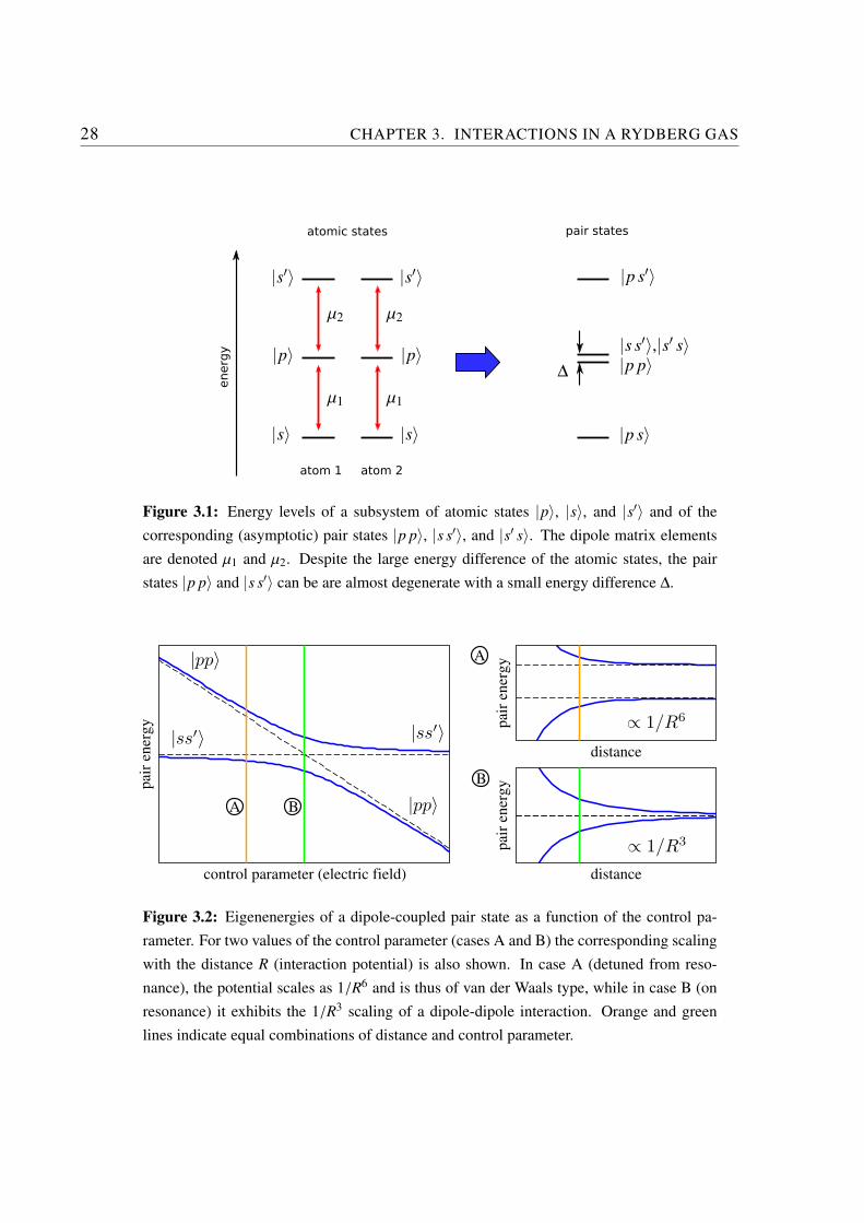
atomic states pair states
atom 1 atom 2
energ
y |p〉|p〉
|s〉|s〉
|s′〉|s′〉 |p s′〉
|p s〉
|p p〉|s s′〉,|s′ s〉
µ1µ1
µ2µ2
∆
Figure 3.1: Energy levels of a subsystem of atomic states |p〉, |s〉, and |s′〉 and of the
corresponding (asymptotic) pair states |p p〉, |s s′〉, and |s′ s〉. The dipole matrix elements
are denoted µ1 and µ2. Despite the large energy difference of the atomic states, the pair
states |p p〉 and |s s′〉 can be are almost degenerate with a small energy difference ∆.
control parameter (electric field)
pai
r en
erg
y
distance
pai
r en
erg
y
distance
pai
r en
erg
y
A
B
A B
|pp〉
|pp〉
|ss′〉 |ss′〉 ∝ 1/R6
∝ 1/R3
Figure 3.2: Eigenenergies of a dipole-coupled pair state as a function of the control pa-
rameter. For two values of the control parameter (cases A and B) the corresponding scaling
with the distance R (interaction potential) is also shown. In case A (detuned from reso-
nance), the potential scales as 1/R6 and is thus of van der Waals type, while in case B (on
resonance) it exhibits the 1/R3 scaling of a dipole-dipole interaction. Orange and green
lines indicate equal combinations of distance and control parameter.
3.1. LONG-RANGE INTERACTIONS 29
where ~R is the distance vector connecting the the two dipoles [Jackson, 1975]. Depending
on the spatial alignment of the dipoles, the interaction can be either attractive or repulsive.
For a quantum-mechanical system, the dipole moment is expressed in terms of the dipole
operator. Its matrix elements 〈ϕ |e~r|ϕ′〉 already been discussed in Sec. 2.2. Consider two
atoms in states |ϕ1〉 and |ϕ2〉. Neglecting the angular dependence of the dipole interaction,
the interaction energy is given by
Vdd(R) ∝1
R3 ∑|ϕ′1〉,|ϕ′2〉
⟨
ϕ1 |µ1|ϕ′1⟩⟨
ϕ2 |µ2|ϕ′2⟩
= ∑|ϕ′1ϕ′2〉
⟨
ϕ1ϕ2
∣
∣
∣
µ1 µ2
R3
∣
∣
∣ϕ′1ϕ′2
⟩
, (3.2)
where the sums extend over all internal states of the two atoms. A simple but instructive
analysis of the dipole interactions is already possible when only the two neighboring
atomic states are included. This simplification is justified by the fact that the dipole matrix
elements between these states are largest. This leads to a subsystem of three atomic levels
as depicted in Fig. 3.1. In the following, the initially populated state is denoted |p〉 and
the two dipole-coupled states are given the names |s〉 and |s′〉. The three atomic states are
energetically well separated. When considering pair states, the states |p p〉 and |s s′〉,|s s′〉are almost degenerate, with an energy gap ∆ as indicated in Fig. 3.1. With the dipole
matrix elements µ1 = 〈p|e~r|s〉 and µ2 = 〈p|e~r|s′〉 the complete Hamiltonian of the subset
(|p p〉 , |s s′〉) can be written
H = HA +Hint =
(
−∆ µ1 µ2
R3
µ1 µ2
R3 0
)
, (3.3)
as the sum of the atomic Hamiltonian HA (with the energy of |p p〉 set to zero), and the
interaction part Hint containing the off-diagonal elements. The new eigenenergies of the
coupled system are
E± = −∆
2±
√
(
∆
2
)2
+(µ1 µ2
R3
)2
. (3.4)
These energies are plotted as functions of ∆ and R in Fig. 3.2. At a detuning of ∆ = 0, the
energies of the new eigenstates |+〉 and |−〉 are split by 2µ1µ2/R3.
In most atomic systems, one has only little influence on the pair state detuning ∆.
Rydberg atoms, however, as a consequence of the enormous Stark shifts, offer a unique
way of tuning the relative position of atomic levels with moderate electric fields. For
some combinations of Rydberg states, even the case ∆ = 0 can be realized. It is therefore
of practical importance to investigate the two limiting cases for very large and very small
values of |∆| (indicated as A and B in Fig. 3.2), which is done in the following.
30 CHAPTER 3. INTERACTIONS IN A RYDBERG GAS
|∆| ≫ |µ1µ2/R3| – van der Waals interaction In the case of a large detuning ∆ (see
case A in Fig. 3.2), Taylor expansion of expression (3.4) yields
E± = −∆
2±(
∆
2+
1
∆
(µ1µ2)2
R6
+ · · ·)
, (3.5)
so that the energy shift of the |pp〉 state is given by
∆E|pp〉 =(µ1 µ2)
2 /∆
R6. (3.6)
This is the van der Waals (induced dipole) interaction energy. With µ ∝ n2 and ∆ ∝ n−3
(see Sec. 2.1) the scaling of the vdW coefficient with the principal quantum number n is
obtained,
C6 = −(µ1 µ2)2
∆∝ n11 . (3.7)
Depending on the sign of ∆, the van der Waals interaction can be either attractive or
repulsive. In the case of rubidium, the high-lying D states exhibit attractive interaction,
while the high-lying S states show repulsive interaction. The van der Waals interaction
plays a central role for the interaction-induced motion discussed in Chapter 4, where
systems of attractively and repulsively interacting atoms are investigated. By considering
a large number of dipole-coupled states with the actual detunings for Rb (or other alkalis),
approximate values for the vdW coefficients can be determined (see for example [Singer
et al., 2005b]).
|∆| ≪ |µ1µ2/R3| – Resonant dipoles When the energy difference ∆ approaches zero
(see case B in Fig. 3.2), the system exhibits a pair state resonance, and Eq. (3.4) reduces
to
E± = ±µ1 µ2
R3= ±C3
R3. (3.8)
The interaction energy now depends on the distance as 1/R−3. In an experiment with al-
kali atoms, such a situation can be achieved for certain settings of the electric field. For ru-
bidium, the pair states |43D5/2〉+ |43D5/2〉 and |41F7/2〉+ |45P3/2〉 are almost degenerate
at zero electric field [Reinhard et al., 2008]. For other pair states, the resonance condition
can be fulfilled at certain offset fields. In cold Rydberg physics this is frequently referred
to as a Forster resonance, in analogy to Forster resonances in biological systems, where a
similar dipole-dipole coupling between molecules is responsible for radiation-less energy
3.1. LONG-RANGE INTERACTIONS 31
-2500
-2000
-1500
-1000
-500
0
0 1 2 3 4 5
energ
y (
MH
z)
distance (µm)
-60
-50
-40
-30
-20
-10
0
10
1.5 2 2.5 3 3.5 4 4.5 5
E−
−C3
R3
C6
R6
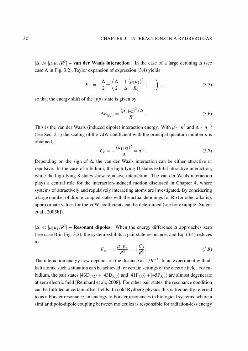
Figure 3.3: Pair interaction potential for the state |32P,32P〉 coupled to |32S,33S〉, with
∆ = −998Mhz (no electric field) and µ1 ≈ µ2 ≈ 1000au. The black solid line is the eigen-
value E−, the red dashed line is the approximation C6/R6 valid for large distances, and the
blue dotted line is of the form −C3/R3, valid for short distances. At typical atomic dis-
tances in the MOT of R > 2µm, the pure van der Waals potential (C6/R6) is a very good
approximation (see inset).
transfer [Forster, 1948, Jares-Erijman and Jovin, 2003]. The interaction strength can ob-
viously be tuned between van der Waals (or induced dipole) interaction of 1/R6 character
and resonant dipole interaction of 1/R3 character. Only a single control parameter is nec-
essary, which, in the case of alkali atoms, can be the electric field. In Sec. 5.3 the energy
transfer resonance is investigated in more detail.
The transition between a C3 and a C6 behavior can of course also be observed when
changing the pair distance instead of the detuning. An example for the energy shift of the
pair state |32P,32P〉 coupled to |32S,33S〉 is presented in Fig. 3.3. (These states are of
particular importance for the energy transfer processes discussed in Sec. 5.3.) In this ex-
ample, no electric field is present and the detuning ∆ is fixed to −998 MHz. Furthermore,
µ1 ≈ µ2 ≈ 1000au for the Rydberg states considered here. In addition to the eigenvalue
E− from Eq. (3.4) (solid black line) the approximations of the form (3.6) (van der Waals
potential, red dashed line) and (3.8) (dipole-dipole potential, blue dotted line) are also
plotted. These approximated potentials intersect at |µ1µ2/R3| = |∆|. For pair distances
R > 2µm, as is typically the case in a MOT, the C6 potential is a very good approxima-
32 CHAPTER 3. INTERACTIONS IN A RYDBERG GAS
tion, as can be seen in the inset of Fig. 3.3.
Rydberg atoms can also acquire permanent dipole moments by polarization in an ex-
ternal electric field. In this case the mixing of different angular momentum states accounts
for a permanent dipole moment, leading to dipole-dipole interaction with R−3 character
among the atoms. As the energy of an electric dipole µ in an electric field E is given by
E =−µ ·E , the dipole moment is represented by the slope of the lines in a Stark map (like
the one shown in Fig. 2.4),
µ(E) = −dE
dE , (3.9)
at the applied electric field E . As already noted in Chapter 2, the polarizability scales
with the principal quantum number as n7 and can thus become very large for high n. This
polarizability in turn leads to extraordinary large dipole moments and accordingly to very
strong dipole interactions. In most experiments presented in this thesis, the effect of the
electric field on state mixing is negligible, so that the dynamics of the system is governed
by van der Waals interaction.
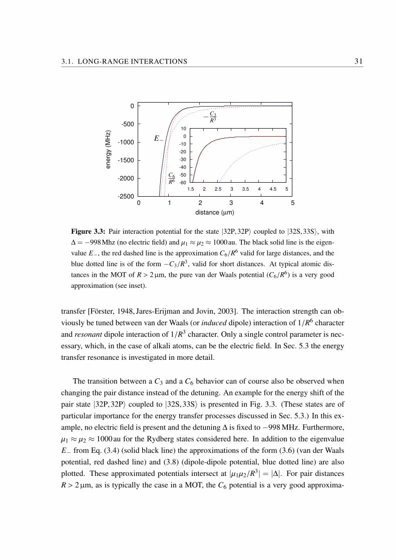
3.1.2 Excitation blockade
The strong long-range interactions between Rydberg atoms can lead to an excitation
blockade, i.e. an inhibition of multiple excitations in a mesoscopic ensemble of atoms.
The effect is caused by the interaction-induced energy shifts and splittings. It is some-
what similar to the Coulomb blockade, where the tunneling of multiple electrons is inhib-
ited [Devoret et al., 1992]. The basic idea of the dipole blockade mechanism is illustrated
in Fig. 3.4: Once an atom is excited to a Rydberg state, no second atom near it can be
excited, because the excitation laser is not resonant any more with the shifted energy
level. The blockade radius Rb is defined as the distance between two atoms at which the
Rydberg interaction energy equals the excitation linewidth:
Vdd(Rb) = γexc (3.10)
Within the region R < Rb around a Rydberg atom no second excitation is possible, as
indicated by the shaded area in Fig. 3.4. This blocked volume is sometimes called a
domain of a single excitation. For typical experimental conditions with laser linewidths
on the oder of 1 MHz, a blockade radius of several µm can be achieved. This is still
small compared to the dimensions of a magneto-optically trapped cloud, so that many
domains are created in the sample. Small dipole traps can be used to traps atoms in
3.1. LONG-RANGE INTERACTIONS 33
(a) (b)
RRb
Energ
y
|gg〉
|gr〉
|rr〉
Figure 3.4: Excitation blockade. (a) A laser tuned to the atomic resonance cannot excite a
second atom within a radius Rb, as the energy level is shifted out of resonance by the inter-
action of the atoms. (b) Illustration of atoms excited in a laser focus. In a simplified picture
several domains of radius Rb are formed, within which only a single Rydberg excitation is
possible.
a sufficiently small volume so that only a single excitation is possible. This technique
has recently been demonstrated [Urban et al., 2008]. The realization of fully blockaded
mesoscopic ensembles is also one prerequisite for the observation of resonant energy
transfer in atom chains, as proposed in Sec. 5.4. A small interacting ensemble of atoms is
correctly described in a multi-particle picture. A mesoscopic cloud of N atoms with all in
the ground state |g〉 is then denoted
|G〉 = |g1 g2 g3 . . .gN〉 . (3.11)
When exciting this multi-particle system, only a single atom can be transferred to the
Rydberg state r. As it is not possible to tell which of the atoms is excited, the state of the
system must then be described as a superposition of many-particle states,
|R〉 =1√N
N
∑i=1
|g1 g2 . . .ri . . .gN−1 gN〉 , (3.12)
where atom i is excited and the other atoms are in their ground states.
In principle, any of the different forms of interaction discussed in Sec. 3.1.1 can cause
an excitation blockade effect, as has been seen in a number of experiments: A blockade
34 CHAPTER 3. INTERACTIONS IN A RYDBERG GAS
was first observed as a suppression of excitation in macroscopic clouds exhibiting strong
van der Waals interaction at high principal quantum numbers [Tong et al., 2004, Singer
et al., 2004]. These measurements showed that the excitation fraction decreases with
increasing density. Later a blockade induced by both resonant and permanent dipoles was
investigated [Vogt et al., 2006,Vogt et al., 2007]. The blockade effect is also accompanied
by a change in counting statistics [Cubel Liebisch et al., 2005].
When exciting this interacting system from the ground state |0〉 to the many-particle
state |R〉 as defined in Eq. (3.12), the Rabi frequency of the transition is modified com-
pared to the Rabi frequency of a single atom [Lukin et al., 2001]. The many-body Rabi
frequency of an N-particle system can be expressed in terms of the atomic Rabi frequency
Ω1 as
ΩN =√NΩ1 . (3.13)
This collective Rabi frequency obviously depends on the number of atoms in the block-
aded ensemble. Although not observed directly, evidence of the modified many-particle
Rabi frequency has recently been found [Heidemann et al., 2007], and the coherent char-
acter of the excitation of a dense interacting sample has been demonstrated [Raitzsch
et al., 2008].
3.2 Pair distribution functions
In order to describe collective behavior of a cloud of atoms, a statistical description of
the distribution of distances is necessary. Especially interesting is the nearest neighbor
distribution, which gives the probability of finding the nearest neighbor of a selected atom
at a given distance.
Consider an atom inside a cloud with a density distribution ρ(~r). Without loss of gen-
erality the atom can be assumed to be at the origin of the coordinate system. In spherical
coordinates, the number of atoms dN found at within the distance interval [r,r+ dr] can
then be expressed as
dN =
[
∫ 2π
0
∫ π
0ρ(ϕ,θ,r)r2 sinθdθdϕ
]
dr . (3.14)
If the density distribution is spherically symmetric around the atom (e.g. the atom is
placed in the center of a magneto-optically trapped cloud), Eq. (3.14) can be integrated,
dN = 4πr2ρ(r)dr . (3.15)
3.2. PAIR DISTRIBUTION FUNCTIONS 35
0
0.5
1
1.5
2
2.5
0 0.2 0.4 0.6 0.8 1 1.2 1.4
r /ρ−1/3
Pnn/ρ
1/3
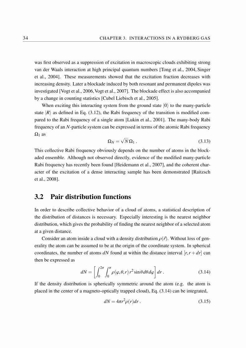
Figure 3.5: Nearest neighbor distribution (3.17) in coordinates scaled by ρ−1/3. The func-
tion rises quadratically in the beginning, as indicated by the dotted line. The maximum of
the curve is found at r ≈ (5/9)ρ−1/3.
Within a volume small enough to assume a constant density, the number of pairs thus
grows with the square of distance.
In many of the phenomena discussed in this work only the interaction with the near-
est neighbor is of interest. It is therefore useful to determine the distribution of nearest
neighbors, i.e. the probability that the nearest neighbor (and not any atom in general) is
found at a given distance. It is assumed that the distribution of atom positions in space
is Poissonian, with a homogeneous density ρ around the atom under consideration. The
probability for finding exactly k atoms in a given volume is then expressed by the Poisson
distribution [Bronstein et al., 2000]
p(k,λ) =λke−λ
k!, (3.16)
where the parameter λ is the average number of particles in this volume. In a sphere of
radius r, the average number of particles is λ = (4/3)πr3ρ. The probability to find the
nearest neighbor of an atom in a spherical shell of radius r and width dr is then given by
the probability for an atom to be found within this volume, 4πr2ρdr, multiplied by the
probability that no atom is inside the sphere of radius r, p(k = 0,λ = (4/3)πr3ρ), which
yields the nearest-neighbor distribution
Pnn(r) = 4πr2ρe−43πρr
3
, (3.17)
plotted in Fig. 3.5. Being a probability density distribution, the nearest-neighbor distribu-
36 CHAPTER 3. INTERACTIONS IN A RYDBERG GAS
tion is normalized,∫ ∞
0Pnn(r)dr = 1 . (3.18)
The most probable nearest neighbor distance (the maximum of the distribution function)
is found from the requirement that
dPnn(r)
dr= 0 (3.19)
which leads to
rmax = 3
√
1
2πρ(3.20)
≈ 0.5419ρ−1/3 . (3.21)
The average nearest neighbor distance is derived by weighting the distances with their
corresponding probabilities:
ravg =∫ ∞
0r×4πρr2e−
43πρr
3
(3.22)
=Γ(1
3)
62/3π1/3ρ1/3(3.23)
≈ 0.5540ρ−1/3 (3.24)
As already pointed out by [Hertz, 1909], both quantities can be approximated by
rmax ≈ ravg ≈5
9ρ−1/3 . (3.25)
This distribution is valid for fully penetrable particles without spatial correlation, and can
be used as an approximation for atoms in a magneto-optical trap or a gas of Rydberg
atoms, provided that the density is not too high. The derivation of similar distribution
functions for hard spheres (instead of fully penetrable particles) can for example be found
in [Torquato et al., 1990, Macdonald, 1992].
It is important to keep in mind that the average distance of neighboring particles in an
unordered gas is not given simply by the cube root of the inverse density, ρ−1/3, as would
be the case for a periodic alignment on a grid.
In many-particle systems where the interaction between the atoms is sufficiently strong,
the pair distribution can be influenced. This is shown in Sec. 4.2, where interaction-
induced line shifts modify the pair distribution during excitation of a Rydberg gas. An
example of how pair distributions change in time while the atoms move due to their inter-
actions is presented in Sec. 4.5.
3.3. INFLUENCE OF SURROUNDING ATOMS 37
3.3 Influence of surrounding atoms
Most investigations of Rydberg systems involve an unordered ensemble of atoms. It is
therefore necessary to estimate the average influence of surrounding atoms on the proper-
ties of single atoms and close atom pairs. In other words, it is important to know when a
description in terms of single atoms or atom pairs is sufficient and in which cases a larger
number of atoms has to be taken into account.
Most distance-dependent quantities considered in this thesis scale as 1/R6 (like the
van der Waals interaction or the resonant dipole-induced ionization rate) or 1/R3 (like the
dipole-dipole interaction). Consider an atom with a nearest neighbor at a distance R0. Let
Q(R) be some quantity depending on the interatomic distance as q/R6 with some constant
q. The value of Qpair for this atom induced by the nearest neighbor only is then given by
Qpair =q
R60
. (3.26)
To estimate the importance of other atoms surrounding the pair, it is assumed that the
quantity is additive and the atom density ρ is constant. An additional contribution Qs
to the quantity under consideration can then be calculated by integrating the pair density
(3.14) from a radius R0 to infinity (as the nearest neighbor is at R0 by definition, all other
atoms must be at larger distance),
Qs =∫ ∞
R0
Ppair(R)Q(R) (3.27)
=∫ ∞
R0
4πR2 ρq
R6dR (3.28)
=4π
3ρq
1
R30
(3.29)
For a homogeneous density ρ the average nearest neighbor distance is given by a =
(5/9)ρ−1/3 (See Eq. (3.25)). For the estimation it is therefore assumed that R0 = a. In
this case ρ can be expressed in terms of R0 which leads to
Qs =4π
3
(
5
9
)3q
R60
(3.30)
≈ 0.718Qpair . (3.31)
The contribution Qs induced by the surrounding of a nearest neighbor pair is therefore
smaller than the value Qpair itself. If an attractive van der Waals interaction (itself scaling
38 CHAPTER 3. INTERACTIONS IN A RYDBERG GAS
as 1/R6) accelerates the atoms towards each other, the nearest neighbors will approach
each other quickly while the surrounding atoms are unaffected by them (refer to Sec. 4.2).
The influence of the surrounding atoms will thus even decrease in a dynamic system.
Another approach to this question is to take the complete distribution of nearest neigh-
bor distances into account. One can compare the total contribution to Q induced on one
atom by all other atoms to the contribution of nearest neighbors, averaging over all possi-
ble nearest neighbor distances for the given density.
The nearest neighbor probability distribution for randomly arranged particles is given
in Eq. (3.17). The average value of Q induced by the nearest neighbor (between distance
R and infinity) can thus be written
Qnn =∫ ∞
RPnn(r)Q(r)dr (3.32)
=4
3πqρ
(
1
R3e−
43πρR
3
+4
3πEi(−4
3πρR3)
)
. (3.33)
Here Ei is the exponential integral function. The sum of the contributions from all sur-
rounding atoms from a distance R to infinity can be expressed similar to Eq. (3.29) by the
integral
Qtotal =∫ ∞
R4πr2ρ Q(r)dr (3.34)
=4
3πqρ
1
R3. (3.35)
Both Qtotal and Qnn diverge in the limit R→ 0 because of the 1/R6 scaling of the quantity
Q. The ratio of Qnn and Qtotal, however, is still a well-defined quantity in this limit:
limR→0
Qnn
Qtotal= 1 (3.36)
Although taking the limit R→ 0 is questionable considering the actual physical system,
this approach leads to the same conclusion, that the value of the Q is mainly determined
by the nearest neighbor while the surrounding atoms do not have significant influence. It
should be noted that Eq. (3.36) is valid not only a 1/R6-dependent quantity, but for all
scalings Q ∝ 1/Rα with α > 3.
These estimations justify to consider a sample of atoms subject to attractive van der
Waals interaction as a collection of nearest-neighbor pairs, as it is assumed in the model
in Sec. 4.2.
3.4. IONIZATION PROCESSES 39
For quantities Q′ scaling as 1/R3 the influence of surrounding atoms becomes signif-
icant. The integral for Q′s derived similar to Eq. (3.29) then diverges and can only be
evaluated with an upper limit Rmax. Expressing the limits of the integral in terms of the
average nearest neighbor distance a as R0 = a and Rmax = βa (β > 1) the integral yields
Q′s = 2.155lnβ Q′
pair (3.37)
where Q′s and Q′
pair now represent arbitrary accumulative quantities scaling as 1/R3. For a
large Rydberg sample in a magneto-optical trap, a value of β= 100 is realistic. In this case
the influence of the surrounding outweighs the nearest neighbor by an order of magnitude.
The different influence of the surrounding for different scaling of the quantity Q is
important for the estimation of interaction-induced energy shifts. In the case of a van der
Waals interaction (1/R6), it may be sufficient to consider only the nearest neighbor (see
for example the excitation model in Sec. 4.1), while the dipole-dipole interaction (1/R3)
requires taking a larger number of atoms into account (an example is the energy transfer
investigated in Sec. 5.3.1).
3.4 Ionization processes
3.4.1 Collisional ionization
Rydberg atoms can be ionized by collisions with other particles. These can be charged
particles like electrons or ions, or other neutral atoms in ground or Rydberg states.
An electron or ion approaching a Rydberg atom can influence the highly polarizable
atom simply with its electric field. Close encounters of Rydberg atoms and electrons
are responsible for n and ℓ changing processes, as the electric field mixes the atomic
states [Dutta et al., 2001]. For high-lying Rydberg states, the electric field of an electron
(or ion) passing a Rydberg atom can even be sufficient to field-ionize the atom. The
electric field at a distance r from a charged particle with charge e is (in SI units)
E =1
4πε0
e
r2. (3.38)
Assuming that the charged particle travels a distance d through a cloud of Rydberg atoms
at a density ρRyd, it will pass
N = πr2 d ρRyd (3.39)
40 CHAPTER 3. INTERACTIONS IN A RYDBERG GAS
Rydberg atoms with an impact parameter smaller than r. Assuming a typical Rydberg
density of ρRyd = 109 cm−3 and a travel distance d = 100µm, an electron can on average
field-ionize 0.58 Rydberg atoms at a principal quantum number of n≈ 80. (The ionization
field is assumed to be ≈ 7.8V/cm according to Eq. (2.21).) The number of Rydberg atoms
redistributed to other states by a passing charged particle can be much higher. A detailed
treatment of ℓ-mixing collisions of hydrogen with ions can be found in [Chibisov, 2007].
Each of the N released electrons will in turn release N secondary electrons, and so forth. If
N < 1, the total increase in the number of ions including the effect of secondary electrons
can therefore be expressed in terms of the geometric progression
∞
∑i=0
Ni =1
1−N, (3.40)
which yields a increase of a factor of 2.4 for the configuration discussed above. For N ≥ 1
the sum diverges and an ionization avalanche takes place. This will be the case when the
electrons are trapped, effectively increasing the interaction distance d (the trapping will
be discussed in Sec. 3.4.4).
At first glance, a collision of two ultracold atoms in the sample seems unlikely be-
cause at the low temperatures of 100µK the atoms can be considered at rest during the
time of observation (typically several µs). This is indeed true if at least one of the atoms is
in its ground state. If both atoms are in Rydberg states, the assumption of a “frozen” gas
does not hold, because the atoms are accelerated due to their strong long-range interaction
potentials. The production of fast Rydberg atoms due to interaction-induced acceleration
has been observed experimentally [Knuffman and Raithel, 2006]. If the interaction is at-
tractive, this can easily lead to a collision within the time scales of observation. Collisions
of Rydberg atoms will almost certainly result in the ionization of one of the collision part-
ners, while the other atom is transferred to a lower Rydberg state [Robicheaux, 2005, Ol-
son, 1979]. This Penning ionization process of two highly excited atoms (X∗∗) can thus
be expressed in the following way:
X∗∗ +X∗∗ → X+ +X∗ + e− (3.41)
Energy conservation demands that the effective principal quantum number of the remain-
ing Rydberg atom (X∗) be reduced by at least a factor of√
2 (this can easily be derived
from Eq. (2.2)). The process of acceleration on attractive pair potentials and subsequent
collision and ionization is illustrated schematically in Fig. 3.6.
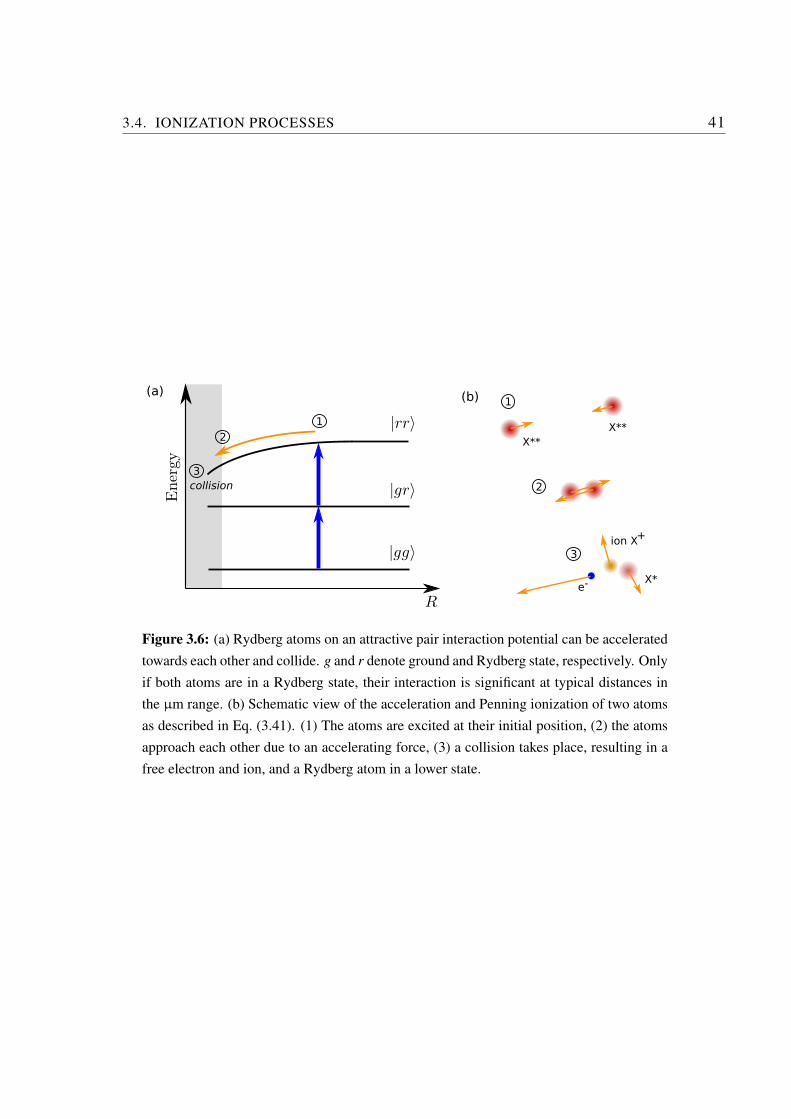
3.4. IONIZATION PROCESSES 41
collision
(a)
e−
ion X
X**
X*
X**
+
(b)
1
1
2
2
3
3
R
Energ
y
|gg〉
|gr〉
|rr〉
Figure 3.6: (a) Rydberg atoms on an attractive pair interaction potential can be accelerated
towards each other and collide. g and r denote ground and Rydberg state, respectively. Only
if both atoms are in a Rydberg state, their interaction is significant at typical distances in
the µm range. (b) Schematic view of the acceleration and Penning ionization of two atoms
as described in Eq. (3.41). (1) The atoms are excited at their initial position, (2) the atoms
approach each other due to an accelerating force, (3) a collision takes place, resulting in a
free electron and ion, and a Rydberg atom in a lower state.
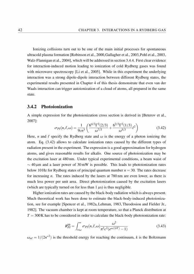
42 CHAPTER 3. INTERACTIONS IN A RYDBERG GAS
Ionizing collisions turn out to be one of the main initial processes for spontaneous
ultracold plasma formation [Robinson et al., 2000,Gallagher et al., 2003,Pohl et al., 2003,
Walz-Flannigan et al., 2004], which will be addressed in section 3.4.4. First clear evidence
for interaction-induced motion leading to ionization of cold Rydberg gases was found
with microwave spectroscopy [Li et al., 2005]. While in this experiment the underlying
interaction was a strong dipole-dipole interaction between different Rydberg states, the
experimental results presented in Chapter 4 of this thesis demonstrate that even van der
Waals interaction can trigger autoionization of a cloud of atoms, all prepared in the same
state.
3.4.2 Photoionization
A simple expression for the photoionization cross section is derived in [Beterov et al.,
2007]:
σPI(n, ℓ,ω) =1
9cn3
(
64/3Γ2(2/3)
ω7/3+
62/3Γ2(1/3)
ω5/3ℓ2
)
(3.42)
Here, n and ℓ specify the Rydberg state and ω is the energy of a photon ionizing the
atom. Eq. (3.42) allows to calculate ionization rates caused by the different types of
radiation present in the experiment. The expression is a good approximation for hydrogen
atoms, and gives reasonable results for alkalis. One source of photoionization may be
the excitation laser at 480 nm. Under typical experimental conditions, a beam waist of
∼ 40µm and a laser power of 30 mW is possible. This leads to photoionization rates
below 10 Hz for Rydberg states of principal quantum number n = 30. The rates decrease
for increasing n. The rates induced by the lasers at 780 nm are even lower, as there is
much less power per unit area. Direct photoionization caused by the excitation lasers
(which are typically turned on for less than 1 µs) is thus negligible.
Higher ionization rates are caused by the black-body radiation which is always present.
Much theoretical work has been done to estimate the black-body-induced photoioniza-
tion, see for example [Spencer et al., 1982a, Lehman, 1983, Theodosiou and Fielder Jr.,
1982]. The vacuum chamber is kept at room temperature, so that a Planck distribution at
T = 300K has to be considered in order to calculate the black-body photoionization rate:
RbbPI =
∫ ∞
ωnℓ
σPI(n, ℓ,ω)ω2
π2c2(eω/(kT )−1)(3.43)
ωnℓ = 1/(2n∗2) is the threshold energy for reaching the continuum, k is the Boltzmann
3.4. IONIZATION PROCESSES 43
0
50
100
150
200
250
300
0 20 40 60 80 100
principal quantum number n
RbbPI
(s−
1)
Figure 3.7: Photoionization rates induced by black-body radiation at T = 300K for rubid-
ium S states (calculated using Eq. (3.44)). The highest rates are found for n≈ 30.
constant, and c is the speed of light. An approximate formula for the integral (3.43) is
again found in [Beterov et al., 2007]:
RbbPI ≈CℓT
(
14423
n∗7/3+
10770ℓ2
n∗11/3
)
× ln
1
1− exp(
−1−157890
Tn∗2
)
s−1 (3.44)
Here Cℓ is an ℓ-dependent factor (CS =CP = 0.2) and T is given in Kelvins. Some values
calculated for S states of rubidium at T = 300K are plotted in Fig. 3.7. The rate peaks at
n≈ 30 and decreases to below 100 s−1 for high principal quantum numbers.
Black-body radiation will also cause redistribution of population among bound states
[Spencer et al., 1982b]. This process will be important for the many-body dynamics in-
vestigated in Sec. 4.3, because the newly populated states induce attractive interactions in
a system initially in repulsive van der Waals states. The transition rate to another Rydberg
state depends on the square of the dipole matrix element connecting these states [Sakurai,
1994]. The largest matrix elements are found between close-lying states (see Sec. 2.2),
which is why the energetically close dipole-coupled states are the ones populated by
black-body radiation. (Note that the spontaneous emission of a Rydberg state is strongest
for final states of low principal quantum number, due to the ω3-dependence of the Ein-
stein A coefficient.) The black-body-induced transition rate from a state |nℓ〉 to a state
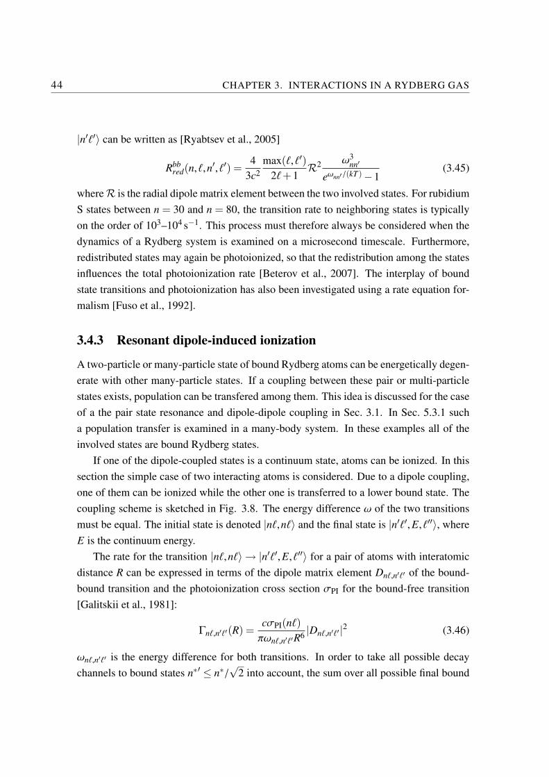
44 CHAPTER 3. INTERACTIONS IN A RYDBERG GAS
|n′ℓ′〉 can be written as [Ryabtsev et al., 2005]
Rbbred(n, ℓ,n
′, ℓ′) =4
3c2
max(ℓ,ℓ′)2ℓ+1
R2 ω3nn′
eωnn′/(kT )−1(3.45)
where R is the radial dipole matrix element between the two involved states. For rubidium
S states between n = 30 and n = 80, the transition rate to neighboring states is typically
on the order of 103–104 s−1. This process must therefore always be considered when the
dynamics of a Rydberg system is examined on a microsecond timescale. Furthermore,
redistributed states may again be photoionized, so that the redistribution among the states
influences the total photoionization rate [Beterov et al., 2007]. The interplay of bound
state transitions and photoionization has also been investigated using a rate equation for-
malism [Fuso et al., 1992].
3.4.3 Resonant dipole-induced ionization
A two-particle or many-particle state of bound Rydberg atoms can be energetically degen-
erate with other many-particle states. If a coupling between these pair or multi-particle
states exists, population can be transfered among them. This idea is discussed for the case
of a the pair state resonance and dipole-dipole coupling in Sec. 3.1. In Sec. 5.3.1 such
a population transfer is examined in a many-body system. In these examples all of the
involved states are bound Rydberg states.
If one of the dipole-coupled states is a continuum state, atoms can be ionized. In this
section the simple case of two interacting atoms is considered. Due to a dipole coupling,
one of them can be ionized while the other one is transferred to a lower bound state. The
coupling scheme is sketched in Fig. 3.8. The energy difference ω of the two transitions
must be equal. The initial state is denoted |nℓ,nℓ〉 and the final state is |n′ℓ′,E, ℓ′′〉, where
E is the continuum energy.
The rate for the transition |nℓ,nℓ〉 → |n′ℓ′,E, ℓ′′〉 for a pair of atoms with interatomic
distance R can be expressed in terms of the dipole matrix element Dnℓ,n′ℓ′ of the bound-
bound transition and the photoionization cross section σPI for the bound-free transition
[Galitskii et al., 1981]:
Γnℓ,n′ℓ′(R) =cσPI(nℓ)
πωnℓ,n′ℓ′R6|Dnℓ,n′ℓ′ |2 (3.46)
ωnℓ,n′ℓ′ is the energy difference for both transitions. In order to take all possible decay
channels to bound states n∗′ ≤ n∗/√
2 into account, the sum over all possible final bound
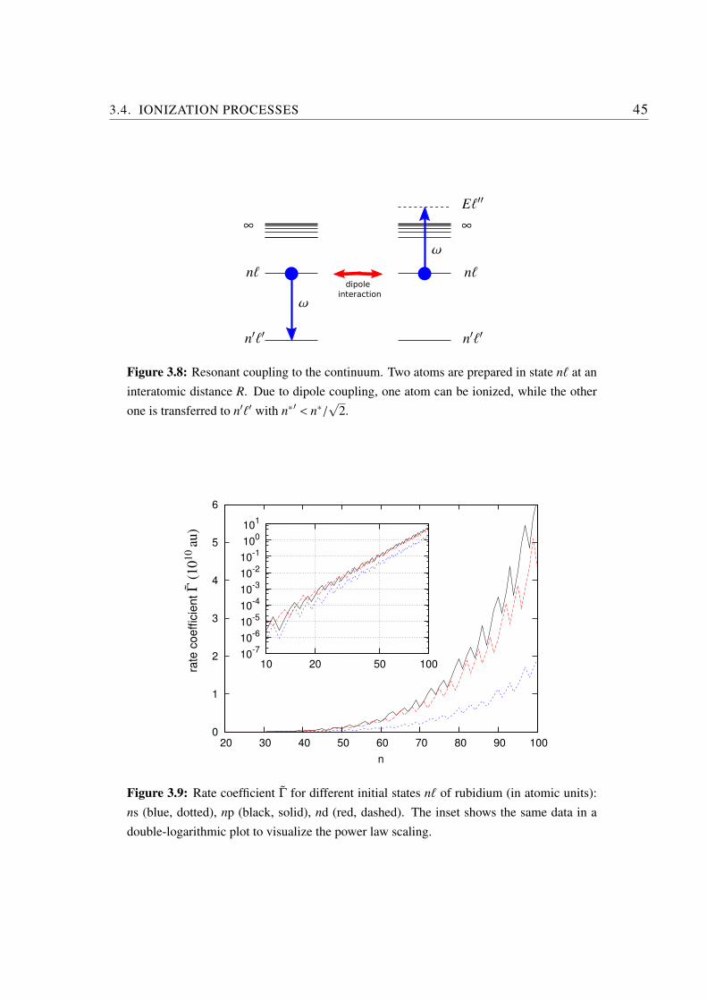
3.4. IONIZATION PROCESSES 45
dipole
interaction
∞∞
nℓnℓ
n′ℓ′n′ℓ′
Eℓ′′
ω
ω
Figure 3.8: Resonant coupling to the continuum. Two atoms are prepared in state nℓ at an
interatomic distance R. Due to dipole coupling, one atom can be ionized, while the other
one is transferred to n′ℓ′ with n∗′ < n∗/√
2.
0
1
2
3
4
5
6
20 30 40 50 60 70 80 90 100
n
10-7
10-6
10-5
10-4
10-3
10-2
10-1
100
101
10 20 50 100rate
coeffi
cie
ntΓ
(10
10
au)
Figure 3.9: Rate coefficient Γ for different initial states nℓ of rubidium (in atomic units):
ns (blue, dotted), np (black, solid), nd (red, dashed). The inset shows the same data in a
double-logarithmic plot to visualize the power law scaling.
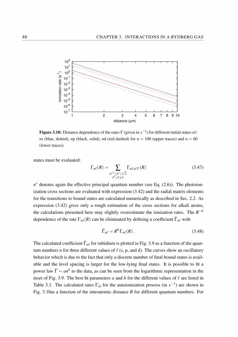
46 CHAPTER 3. INTERACTIONS IN A RYDBERG GAS
10-7
10-6
10-5
10-4
10-3
10-2
10-1
100
101
102
1 2 3 4 5 6 7 8 9 10
ioniz
ation r
ate
(s
-1)
distance (µm)
Figure 3.10: Distance dependence of the rates Γ (given in s−1) for different initial states nℓ:
ns (blue, dotted), np (black, solid), nd (red dashed) for n = 100 (upper traces) and n = 60
(lower traces).
states must be evaluated:
Γnℓ(R) = ∑n∗′≤n∗/
√2
ℓ′=ℓ±1
Γnℓ,n′ℓ′(R) (3.47)
n∗ denotes again the effective principal quantum number (see Eq. (2.6)). The photoion-
ization cross sections are evaluated with expression (3.42) and the radial matrix elements
for the transitions to bound states are calculated numerically as described in Sec. 2.2. As
expression (3.42) gives only a rough estimation of the cross sections for alkali atoms,
the calculations presented here may slightly overestimate the ionization rates. The R−6
dependence of the rate Γnℓ(R) can be eliminated by defining a coefficient Γnℓ with
Γnℓ = R6 Γnℓ(R) . (3.48)
The calculated coefficient Γnℓ for rubidium is plotted in Fig. 3.9 as a function of the quan-
tum numbers n for three different values of ℓ (s, p, and d). The curves show an oscillatory
behavior which is due to the fact that only a discrete number of final bound states is avail-
able and the level spacing is larger for the low-lying final states. It is possible to fit a
power law Γ = anb to the data, as can be seen from the logarithmic representation in the
inset of Fig. 3.9. The best fit parameters a and b for the different values of ℓ are listed in
Table 3.1. The calculated rates Γnl for the autoionization process (in s−1) are shown in
Fig. 3.10as a function of the interatomic distance R for different quantum numbers. For
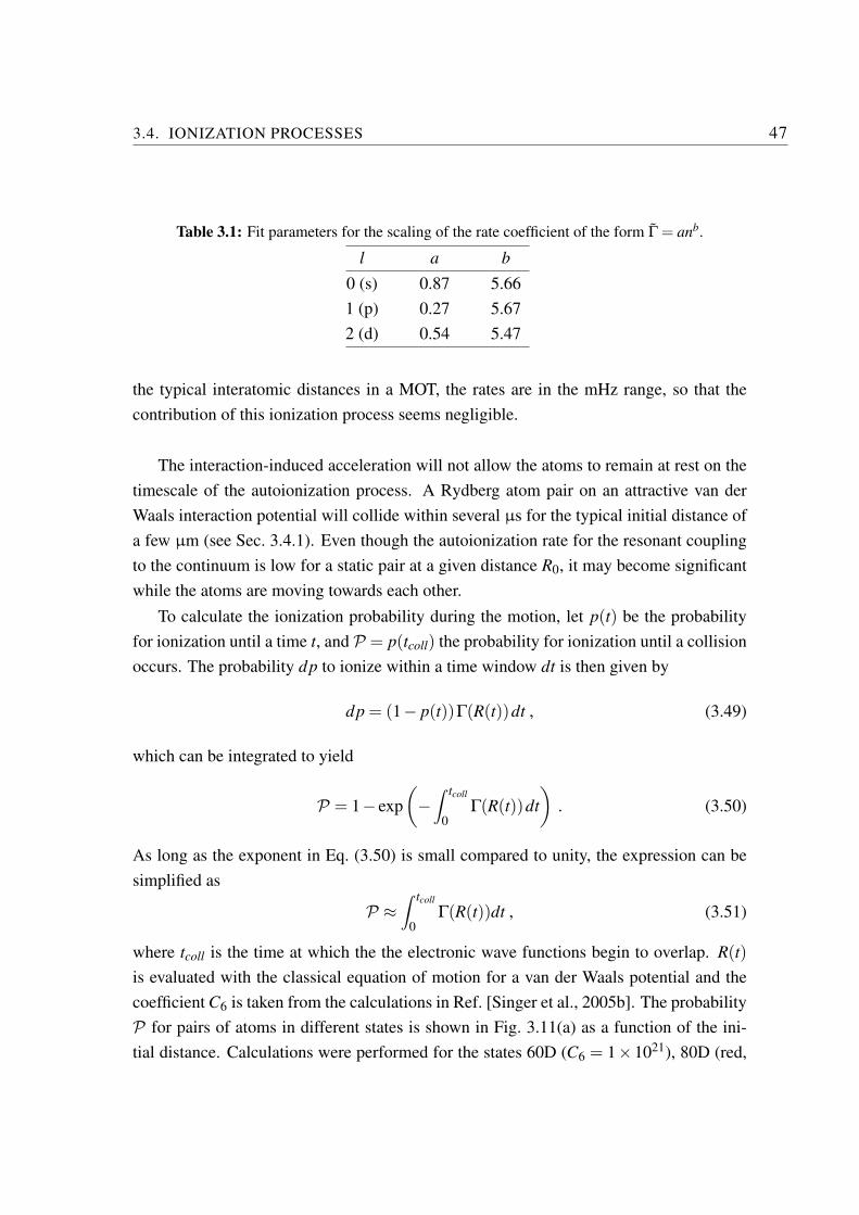
3.4. IONIZATION PROCESSES 47
Table 3.1: Fit parameters for the scaling of the rate coefficient of the form Γ = anb.
l a b
0 (s) 0.87 5.66
1 (p) 0.27 5.67
2 (d) 0.54 5.47
the typical interatomic distances in a MOT, the rates are in the mHz range, so that the
contribution of this ionization process seems negligible.
The interaction-induced acceleration will not allow the atoms to remain at rest on the
timescale of the autoionization process. A Rydberg atom pair on an attractive van der
Waals interaction potential will collide within several µs for the typical initial distance of
a few µm (see Sec. 3.4.1). Even though the autoionization rate for the resonant coupling
to the continuum is low for a static pair at a given distance R0, it may become significant
while the atoms are moving towards each other.
To calculate the ionization probability during the motion, let p(t) be the probability
for ionization until a time t, and P = p(tcoll) the probability for ionization until a collision
occurs. The probability dp to ionize within a time window dt is then given by
dp = (1− p(t))Γ(R(t))dt , (3.49)
which can be integrated to yield
P = 1− exp
(
−∫ tcoll
0Γ(R(t))dt
)
. (3.50)
As long as the exponent in Eq. (3.50) is small compared to unity, the expression can be
simplified as
P ≈∫ tcoll
0Γ(R(t))dt , (3.51)
where tcoll is the time at which the the electronic wave functions begin to overlap. R(t)
is evaluated with the classical equation of motion for a van der Waals potential and the
coefficient C6 is taken from the calculations in Ref. [Singer et al., 2005b]. The probability
P for pairs of atoms in different states is shown in Fig. 3.11(a) as a function of the ini-
tial distance. Calculations were performed for the states 60D (C6 = 1×10²¹), 80D (red,
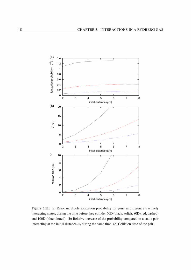
48 CHAPTER 3. INTERACTIONS IN A RYDBERG GAS
0
0.2
0.4
0.6
0.8
1
1.2
1.4
2 3 4 5 6 7 8
ion
iza
tio
n p
rob
ab
ility
(1
0-8
)
inital distance (µm)
(a)
0
5
10
15
20
2 3 4 5 6 7 8
inital distance (µm)
(b)
0
2
4
6
8
10
2 3 4 5 6 7 8
co
llisio
n t
ime
(µ
s)
inital distance (µm)
(c)
P/P
0
Figure 3.11: (a) Resonant dipole ionization probability for pairs in different attractively
interacting states, during the time before they collide: 60D (black, solid), 80D (red, dashed)
and 100D (blue, dotted). (b) Relative increase of the probability compared to a static pair
interacting at the initial distance R0 during the same time. (c) Collision time of the pair.
3.4. IONIZATION PROCESSES 49
C6 = 2.4×10²²), and 100D (red, C6 = 2.8×10²³). For the given probabilities, the obser-
vation time must obviously be at least as long as the collision time plotted in Fig. 3.11(c).
For a limited observation time the rates will decrease again with increasing R0. Despite
the higher value of Γ for increasing principal quantum number n, the ionization proba-
bility decreases, as the atoms spend only a short time in close proximity to each other
before they collide. With P0 = Γ(R(0))tcoll the ionization probability for a static pair
interacting during the same time tcoll, the relative probability P/P0 can be obtained (see
Fig. 3.11(b)). For typical initial distances the attractive motion increases the ionization
probability before a collision by an order of magnitude compared to the static pair.
If the pair of atoms under consideration is a nearest neighbor pair embedded in a
larger ensemble of atoms, the above estimations for attractive interaction are still valid
without taking the surrounding atoms into account (see Sec. 3.3 for a justification). If the
atoms are prepared in states exhibiting repulsive interaction, however, the dynamics of
the whole sample of atoms must be considered. The ionization probability for an isolated
pair is small, as the atoms are drawn apart immediately. When the pair is surrounded
by a cloud of many atoms, each of the two initial partners will come into the vicinity of
other atoms several times while moving across the cloud [Amthor et al., 2007a]. In this
way the ionization probability of this specific atom increases compared to the situation
where only one partner atom is present. For the description of this dynamic system, the
ionization probability is expressed as a function of time, P = P(t). The ionization prob-
ability P(t) for an atom pair in the 60S state is shown in Fig. 3.12. Two isolated atoms
in free space will be accelerated and move away from each other, so that the ionization
probability reaches a steady-state value. When the same nearest-neighbor pair is placed
in the middle of a large atom cloud, the probability that one of the initial partners ionized
is increasing steadily in time, as both atoms come close to other particles while moving
away from each other. The simulations shown here are based on a Monte Carlo model
similar to the one described in Sec. 4.3. For a cloud of randomly placed Rydberg atoms
the equations of motion for all particles are solved, assuming repulsive interaction poten-
tials with C6 = −1021 au. The results are averaged over 50 runs of the simulation. In the
calculation presented in Fig. 3.12, a Rydberg density of 1.5× 109 cm−3 is assumed. For
a typical nearest-neighbor distance of ∼ 4µm the ionization rate of a pair is enhanced by
the surrounding atoms by roughly a factor of 1.4.
Even when many-particle systems are considered, the ionization probability induced
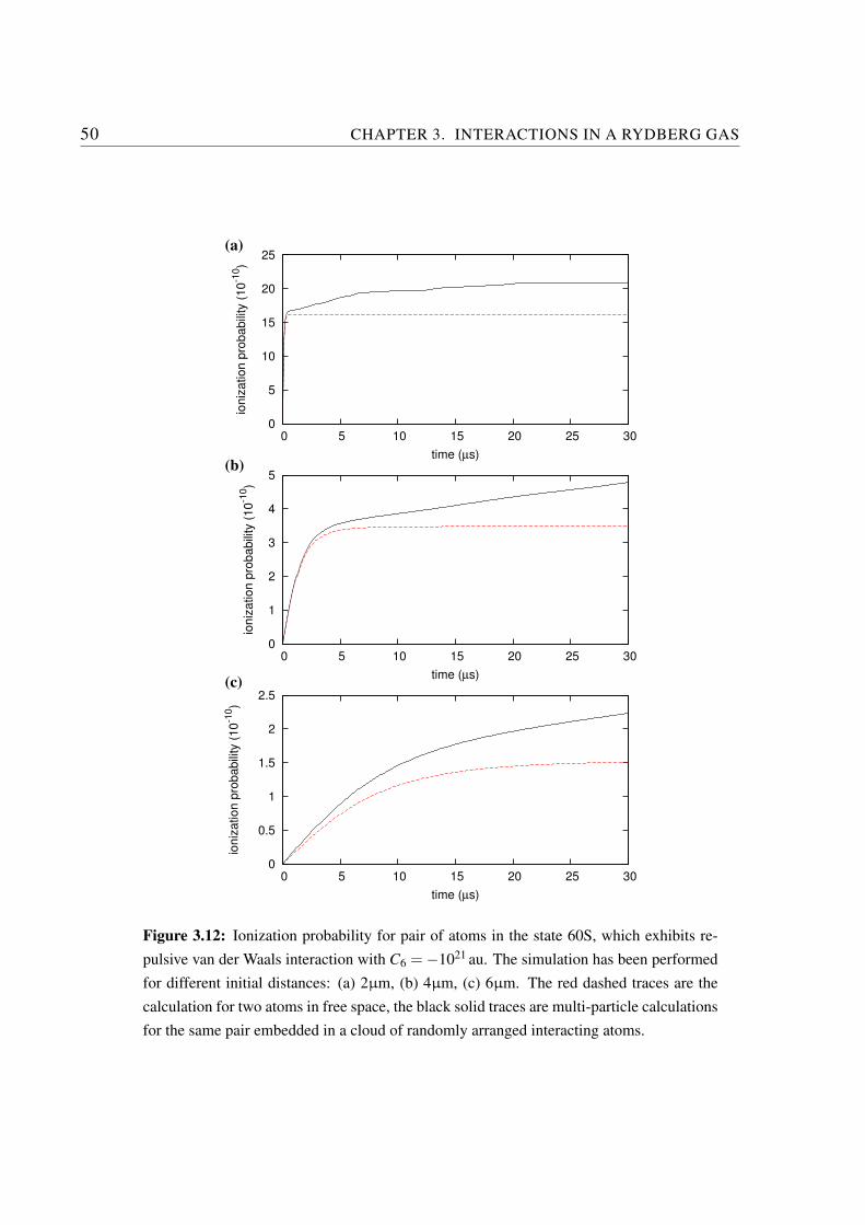
50 CHAPTER 3. INTERACTIONS IN A RYDBERG GAS
0
5
10
15
20
25
0 5 10 15 20 25 30
ion
iza
tio
n p
rob
ab
ility
(1
0-1
0)
time (µs)
(a)
0
1
2
3
4
5
0 5 10 15 20 25 30
ion
iza
tio
n p
rob
ab
ility
(1
0-1
0)
time (µs)
(b)
0
0.5
1
1.5
2
2.5
0 5 10 15 20 25 30
ion
iza
tio
n p
rob
ab
ility
(1
0-1
0)
time (µs)
(c)
Figure 3.12: Ionization probability for pair of atoms in the state 60S, which exhibits re-
pulsive van der Waals interaction with C6 = −1021 au. The simulation has been performed
for different initial distances: (a) 2µm, (b) 4µm, (c) 6µm. The red dashed traces are the
calculation for two atoms in free space, the black solid traces are multi-particle calculations
for the same pair embedded in a cloud of randomly arranged interacting atoms.
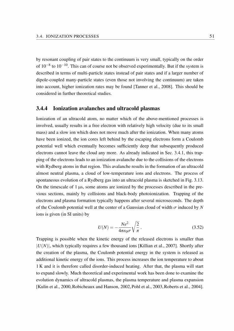
3.4. IONIZATION PROCESSES 51
by resonant coupling of pair states to the continuum is very small, typically on the order
of 10−8 to 10−10. This can of course not be observed experimentally. But if the system is
described in terms of multi-particle states instead of pair states and if a larger number of
dipole-coupled many-particle states (even those not involving the continuum) are taken
into account, higher ionization rates may be found [Tanner et al., 2008]. This should be
considered in further theoretical studies.
3.4.4 Ionization avalanches and ultracold plasmas
Ionization of an ultracold atom, no matter which of the above-mentioned processes is
involved, usually results in a free electron with relatively high velocity (due to its small
mass) and a slow ion which does not move much after the ionization. When many atoms
have been ionized, the ion cores left behind by the escaping electrons form a Coulomb
potential well which eventually becomes sufficiently deep that subsequently produced
electrons cannot leave the cloud any more. As already indicated in Sec. 3.4.1, this trap-
ping of the electrons leads to an ionization avalanche due to the collisions of the electrons
with Rydberg atoms in that region. This avalanche results in the formation of an ultracold
almost neutral plasma, a cloud of low-temperature ions and electrons. The process of
spontaneous evolution of a Rydberg gas into an ultracold plasma is sketched in Fig. 3.13.
On the timescale of 1 µs, some atoms are ionized by the processes described in the pre-
vious sections, mainly by collisions and black-body photoionization. Trapping of the
electrons and plasma formation typically happens after several microseconds. The depth
of the Coulomb potential well at the center of a Gaussian cloud of width σ induced by N
ions is given (in SI units) by
U(N) = − Ne2
4πε0σ
√
2
π. (3.52)
Trapping is possible when the kinetic energy of the released electrons is smaller than
|U(N)|, which typically requires a few thousand ions [Killian et al., 2007]. Shortly after
the creation of the plasma, the Coulomb potential energy in the system is released as
additional kinetic energy of the ions. This process increases the ion temperature to about
1 K and it is therefore called disorder-induced heating. After that, the plasma will start
to expand slowly. Much theoretical and experimental work has been done to examine the
evolution dynamics of ultracold plasmas, the plasma temperature and plasma expansion
[Kulin et al., 2000,Robicheaux and Hanson, 2002,Pohl et al., 2003,Roberts et al., 2004].
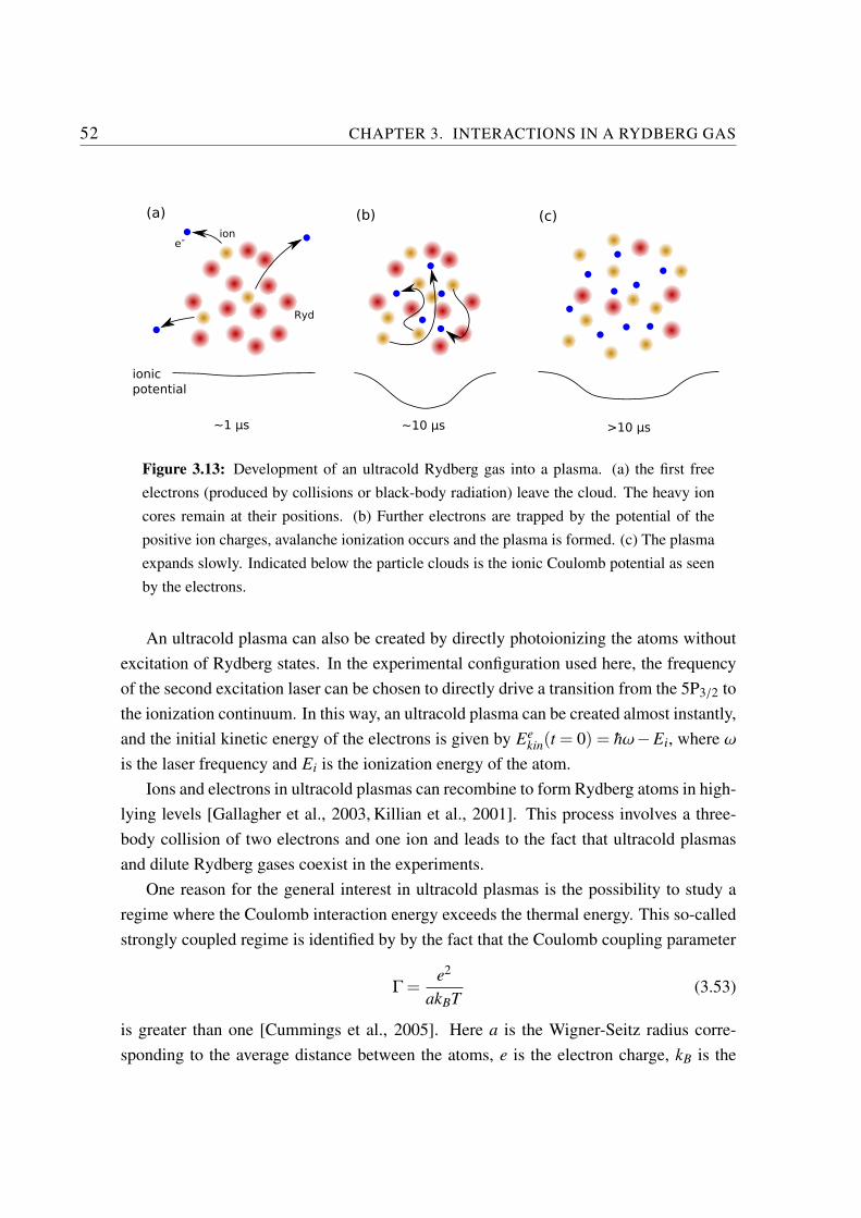
52 CHAPTER 3. INTERACTIONS IN A RYDBERG GAS
(a) (b) (c)
e−
Ryd
ion
ionic
potential
~1 µs ~10 µs >10 µs
Figure 3.13: Development of an ultracold Rydberg gas into a plasma. (a) the first free
electrons (produced by collisions or black-body radiation) leave the cloud. The heavy ion
cores remain at their positions. (b) Further electrons are trapped by the potential of the
positive ion charges, avalanche ionization occurs and the plasma is formed. (c) The plasma
expands slowly. Indicated below the particle clouds is the ionic Coulomb potential as seen
by the electrons.
An ultracold plasma can also be created by directly photoionizing the atoms without
excitation of Rydberg states. In the experimental configuration used here, the frequency
of the second excitation laser can be chosen to directly drive a transition from the 5P3/2 to
the ionization continuum. In this way, an ultracold plasma can be created almost instantly,
and the initial kinetic energy of the electrons is given by Eekin(t = 0) = hω−Ei, where ω
is the laser frequency and Ei is the ionization energy of the atom.
Ions and electrons in ultracold plasmas can recombine to form Rydberg atoms in high-
lying levels [Gallagher et al., 2003, Killian et al., 2001]. This process involves a three-
body collision of two electrons and one ion and leads to the fact that ultracold plasmas
and dilute Rydberg gases coexist in the experiments.
One reason for the general interest in ultracold plasmas is the possibility to study a
regime where the Coulomb interaction energy exceeds the thermal energy. This so-called
strongly coupled regime is identified by by the fact that the Coulomb coupling parameter
Γ =e2
akBT(3.53)
is greater than one [Cummings et al., 2005]. Here a is the Wigner-Seitz radius corre-
sponding to the average distance between the atoms, e is the electron charge, kB is the
3.4. IONIZATION PROCESSES 53
Boltzmann constant, and T is the temperature. In the case Γ ≪ 1 the plasma is called
weakly coupled. In the strongly coupled regime, spatial correlations among the particles
should be expected. Being themselves fascinating objects to study, these systems are also
of interest for other research areas investigating dense plasmas, such as astrophysics. The
physics of ultracold plasmas is reviewed in detail in [Killian, 2007, Killian et al., 2007].
3.4.5 Anion formation
In addition to the formation of positive ions by removal of the highly excited electron as
described in the previous sections, it is also possible that a neutral atom captures a free
electron from a plasma or a weakly bound electron from a Rydberg atom, thereby form-
ing a negative ion (anion). Transfer of Rydberg electrons to other atoms or molecules has
been observed in collision experiments, for example the charge transfer between xenon
Rydberg atoms and SF6 molecules [West et al., 1976], or the charge transfer from a Ryd-
berg atom to another Rydberg or ground state atom in a hot thermal gas [Cheret and
Barbier, 1984, Ciocca et al., 1986]. These observations raise the question as to whether
anions can be formed in a gas of ultracold atoms. In the following, the possible anion
formation processes in a system of ultracold rubidium atoms are discussed.
Anion formation in an ultracold plasma Starting from an ultracold plasma, a free
electron could be captured by a Rydberg or ground state atom:
Rb∗ + e− → Rb− + Ekin (3.54)
Rb + e− → Rb− + Ekin (3.55)
where Rb∗ denotes a Rydberg atom and Ekin is the excess energy converted to kinetic
energy of the involved particles.
Anion formation in an ultracold Rydberg gas In a cloud of highly excited neutral
atoms, a Rydberg electron can be transferred to another neutral atom, which itself is in
either a Rydberg or ground state:
Rb∗ + Rb∗ → Rb+ + Rb− + Ekin (3.56)
Rb∗ + Rb → Rb+ + Rb− + Ekin (3.57)
54 CHAPTER 3. INTERACTIONS IN A RYDBERG GAS
Estimations of the expected anion formation rate can be made with the expressions derived
by [Cheret and Barbier, 1984] and [Ciocca et al., 1986] for hot gases. The temperature
dependence of the anion formation rate k− is given by [Cheret and Barbier, 1984]
k− =∫ ∞
0σ f (v)vdv , (3.58)
where f (v) is the Maxwellian velocity distribution (in SI units) [Atkins, 1998]
f (v) = 4π
(
mRb
2πkBT
)3/2
v2 exp
(
−mRbv2
2kBT
)
(3.59)
and σ is the cross section of the process, which is approximated by the orbital cross
section of the Rydberg atom, σ≈ π(a0n2)2. For the Rydberg state with n = 20 discussed
by [Cheret and Barbier, 1984], a calculation yields k− = 3.8× 10⁻¹³ m3/s for a room
temperature gas (T = 300K), and k− = 2.2× 10⁻¹⁶ m3/s for an ultracold gas with T =
100µK. Considering that the number of anions N− produced per laser shot depends on
the square of the Rydberg density ρRyd,
N− ∝ ρ2Rydk
− , (3.60)
and the fact that the typical Rydberg density in an ultracold cloud is four orders of mag-
nitude smaller than the density of the hot vapor used by [Cheret and Barbier, 1984], the
total expected number of anions in the ultracold gas is eleven orders of magnitude smaller.
Provided that expression (3.58) is still valid in the ultracold regime, the observation of an-
ions in an ultracold gas is very improbable.
In an experiment to search for anions, the electric field configuration was inverted
with respect to the normal positive ion detection described in Sec. 2.4. In this way, nega-
tively charged particles (electrons and anions) could be detected by the MCP detector. A
detailed description of the experimental setup is given in [Hofmann, 2008]. Knowledge
of all static and time-dependent electric fields applied to the electrodes in the setup allows
to calculate the trajectories of anions. In this way, a time window for the expected arrival
of anions on the MCP detector could be determined. Experiments have been performed
with both a gas of highly excited Rydberg atoms and an ultracold plasma produced by
photoionization [Hofmann, 2008]. Despite the high sensitivity of the ion detection, no
evidence for anions could be found in any of the experiments. This supports the assump-
tion that the probability for anion production in ultracold gases is indeed very low.
Chapter 4
Mechanical effects of Rydberg
interactions
Rydberg atoms interact over large distances and interaction energies at typical interatomic
separations in a magneto-optical trap outweigh the thermal energy of the atoms. On a
timescale of microseconds, cold atoms confined in the trap can usually be assumed to be
at rest. Atoms excited to Rydberg levels exert forces on each other, given by the gradient
of the long-range interaction potentials. The atoms are thus accelerated and gain kinetic
energy. The interaction can be either attractive or repulsive, depending on the Rydberg
state chosen. Atom pairs on attractive interaction potentials can approach each other
quickly and even collide on the typical experimental time scales of several microseconds.
The assumption of a frozen gas is thus not always valid.
Motion and ionizing collisions of the atoms must be well understood and considered
in many experiments, because these effects may completely determine the dynamics of
the system, introduce decoherence, and change the interaction strengths. In the following
sections, the mechanical effects of the interaction are investigated in detail for different
interaction potentials. Ionizing collisions serve as a tool to observe the motion of the
atoms in real time. All experimental observations are compared to Monte Carlo models
of interacting Rydberg gases. These comparisons can even provide information on the
interaction strength. Using different configurations of detuned Rydberg excitation, it is
demonstrated that the pair distribution and the collision dynamics can be controlled to
some degree. The simulations have been coded in C and run on a standard Pentium
processor system.
55
56 CHAPTER 4. MECHANICAL EFFECTS OF RYDBERG INTERACTIONS
4.1 Monte-Carlo excitation model
For the investigation of the motion and collision dynamics of a gas of Rydberg atoms it is
essential to know the exact distribution of distances in the cloud directly after the excita-
tion. Due to the strong long-range interaction of Rydberg states, the excitation probability
of the atoms is influenced by surrounding Rydberg atoms which leads to effects such as
suppression of excitation and variations in the pair distribution.
A simple description of a semiclassical excitation rate taking into account the energy
shift on an attractive dipole potential has been discussed by [Gallagher and Pritchard,
1989]. In this work, the authors derive the probability to excite a pair of Na(3S 1/2) atoms
to a Na(3S 1/2)–Na(3P3/2) pair. In this case a bath of ground state atoms is available and
only one atom of a pair is excited. As long as only few ground state–excited state pairs
are created, the density of ground state atoms can be assumed to be homogeneous and
constant in time, and the excitation probability for an atom at a distance R from another
atom can be expressed as
Ppair(R) ∝ 4πR2L(δ−V(R)) (4.1)
where 4πR2 is the density of pairs (see Section 3.2) and L is a Lorentzian line shape of the
excitation shifted by the interaction energy at the given pair distance. This description of
the excitation process is only possible if the involved interaction is between a ground state
and an excited state atom and the density of excited atoms is not too high. In the case of
an excitation of a cold gas to Rydberg states the interaction to be considered is between
the excited atoms only, while the Rydberg–ground state interaction can be neglected. In
other words, the density of the atoms to be considered as interaction partners is not con-
stant in time, as more and more Rydberg atoms are excited. The simple description in
terms of a pair distribution at a known density is not appropriate for Rydberg excitation.
Instead, the excitation process must be modeled with a Monte Carlo algorithm, to deter-
mine the excitation probability of a specific atom at a given time, taking into account the
interaction-induced line shift of neighboring Rydberg atoms.
The calculations shown in this chapter are based on the following algorithm. First,
5000 atoms are randomly placed in space to represent a density of 1010 cm−3 which corre-
sponds to the typical density at the center of the MOT. The excitation model is an iterative
process. In each iteration step, each of the atoms has a certain probability for excitation
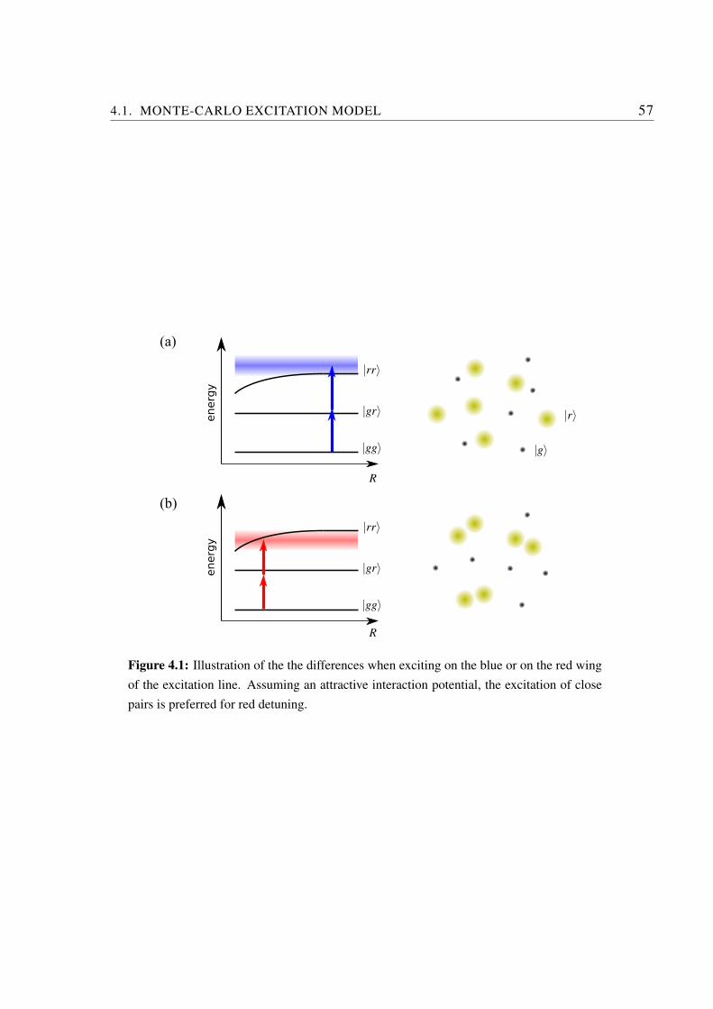
4.1. MONTE-CARLO EXCITATION MODEL 57
(a)
(b)
energ
yenerg
y
|rr〉
|rr〉
|gr〉
|gr〉
|gg〉
|gg〉
R
R
|g〉
|r〉
Figure 4.1: Illustration of the the differences when exciting on the blue or on the red wing
of the excitation line. Assuming an attractive interaction potential, the excitation of close
pairs is preferred for red detuning.
58 CHAPTER 4. MECHANICAL EFFECTS OF RYDBERG INTERACTIONS
or stimulated emission. For atom i, this probability reads
Pi = aL(δ−VvdW(Ri))e−2(x2
i +y2i )/w
2
. (4.2)
L represents the laser line shape, determined by the width of the intermediate state 5P
(6 MHz FWHM), the widths of the two lasers (1–2 MHz), and the Fourier transform of
the excitation pulse (∼3 MHz FWHM). The Rydberg excitation line can usually be ap-
proximated reasonably well by a Lorentzian, which is why
L(x) =(Γ
2)2
x2 +(Γ2)2
(4.3)
is a Lorentzian in all the simulations presented here, Γ being the width of the distribu-
tion. It is evaluated at a detuning δ (the detuning of the laser from resonance), and also
takes an interaction-induced line shift into account. This van der Waals interaction energy
VvdW(Ri) is determined by the interaction with the nearest Rydberg neighbor. The last
factor accounts for the Gaussian intensity distribution of the excitation laser. Assigning
the factor a a small value (a = 0.001) ensures that only a small number of excitations
occur in each iteration step and the outcome of the simulation is independent of the or-
der in which the atoms are addressed. The procedure is iterated several hundred times
until the actual percentage of excited atoms observed in the experiment is reached (typi-
cally 10–30% at δ = 0). For each atom, the distance Ri to its nearest Rydberg neighbor
is recalculated after each excitation or stimulated emission event. The restriction to the
nearest neighbor when determining the interaction-induced line shift can be justified with
the arguments presented in Sec. 3.3, as the van der Waals interactions scales as 1/R6.
Fig. 4.1 illustrates the difference of excitation for blue and red detuning of the ex-
citation laser on an attractive interaction potential. While for blue detuning atoms are
excited at larger separation, a red detuning enhances the excitation of close pairs, as the
Rydberg–Rydberg interaction shifts the energy level into resonance with the laser for
small separations. Even though the total number of excited atoms in this illustration is the
same for both detunings, the distribution of pair distances differs.
4.2 Dynamics of attractive Rydberg systems
Given an attractive van der Waals potential, Rydberg atoms are influenced mostly by their
nearest neighbor, and when the atoms start to move towards each other, the influence
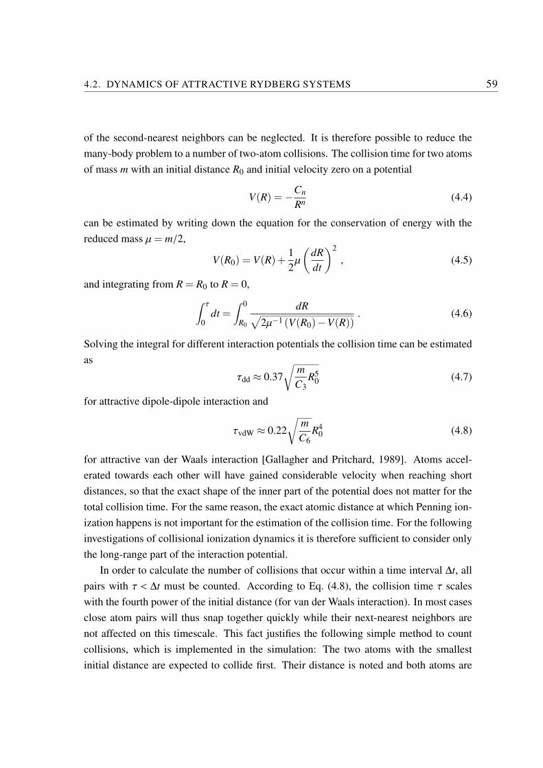
4.2. DYNAMICS OF ATTRACTIVE RYDBERG SYSTEMS 59
of the second-nearest neighbors can be neglected. It is therefore possible to reduce the
many-body problem to a number of two-atom collisions. The collision time for two atoms
of mass m with an initial distance R0 and initial velocity zero on a potential
V(R) = −Cn
Rn(4.4)
can be estimated by writing down the equation for the conservation of energy with the
reduced mass µ= m/2,
V(R0) = V(R)+1
2µ
(
dR
dt
)2
, (4.5)
and integrating from R = R0 to R = 0,
∫ τ
0dt =
∫ 0
R0
dR√
2µ−1 (V(R0)−V(R)). (4.6)
Solving the integral for different interaction potentials the collision time can be estimated
as
τdd ≈ 0.37
√
m
C3R5
0 (4.7)
for attractive dipole-dipole interaction and
τvdW ≈ 0.22
√
m
C6
R40 (4.8)
for attractive van der Waals interaction [Gallagher and Pritchard, 1989]. Atoms accel-
erated towards each other will have gained considerable velocity when reaching short
distances, so that the exact shape of the inner part of the potential does not matter for the
total collision time. For the same reason, the exact atomic distance at which Penning ion-
ization happens is not important for the estimation of the collision time. For the following
investigations of collisional ionization dynamics it is therefore sufficient to consider only
the long-range part of the interaction potential.
In order to calculate the number of collisions that occur within a time interval ∆t, all
pairs with τ < ∆t must be counted. According to Eq. (4.8), the collision time τ scales
with the fourth power of the initial distance (for van der Waals interaction). In most cases
close atom pairs will thus snap together quickly while their next-nearest neighbors are
not affected on this timescale. This fact justifies the following simple method to count
collisions, which is implemented in the simulation: The two atoms with the smallest
initial distance are expected to collide first. Their distance is noted and both atoms are
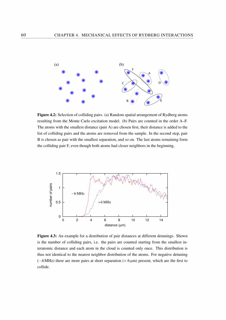
60 CHAPTER 4. MECHANICAL EFFECTS OF RYDBERG INTERACTIONS
A
B
C D
E
F
(a) (b)
Figure 4.2: Selection of colliding pairs. (a) Random spatial arrangement of Rydberg atoms
resulting from the Monte Carlo excitation model. (b) Pairs are counted in the order A–F.
The atoms with the smallest distance (pair A) are chosen first, their distance is added to the
list of colliding pairs and the atoms are removed from the sample. In the second step, pair
B is chosen as pair with the smallest separation, and so on. The last atoms remaining form
the colliding pair F, even though both atoms had closer neighbors in the beginning.
0
0.5
1
1.5
0 2 4 6 8 10 12 14
num
ber
of
pairs
distance (µm)
−6 MHz
+6 MHz
Figure 4.3: An example for a distribution of pair distances at different detunings. Shown
is the number of colliding pairs, i.e. the pairs are counted starting from the smallest in-
teratomic distance and each atom in the cloud is counted only once. This distribution is
thus not identical to the nearest neighbor distribution of the atoms. For negative detuning
(−6MHz) there are more pairs at short separation (< 6µm) present, which are the first to
collide.
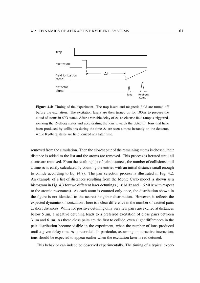
4.2. DYNAMICS OF ATTRACTIVE RYDBERG SYSTEMS 61
excitation
field ionization
ramp
trap
detector
signal
ions Rydberg
atoms
∆t
Figure 4.4: Timing of the experiment. The trap lasers and magnetic field are turned off
before the excitation. The excitation lasers are then turned on for 100 ns to prepare the
cloud of atoms in 60D states. After a variable delay of ∆t, an electric field ramp is triggered,
ionizing the Rydberg states and accelerating the ions towards the detector. Ions that have
been produced by collisions during the time ∆t are seen almost instantly on the detector,
while Rydberg states are field ionized at a later time.
removed from the simulation. Then the closest pair of the remaining atoms is chosen, their
distance is added to the list and the atoms are removed. This process is iterated until all
atoms are removed. From the resulting list of pair distances, the number of collisions until
a time ∆t is easily calculated by counting the entries with an initial distance small enough
to collide according to Eq. (4.8). The pair selection process is illustrated in Fig. 4.2.
An example of a list of distances resulting from the Monte Carlo model is shown as a
histogram in Fig. 4.3 for two different laser detunings (−6 MHz and +6 MHz with respect
to the atomic resonance). As each atom is counted only once, the distribution shown in
the figure is not identical to the nearest-neighbor distribution. However, it reflects the
expected dynamics of ionization There is a clear difference in the number of excited pairs
at short distances. While for positive detuning only very few pairs are excited at distances
below 5µm, a negative detuning leads to a preferred excitation of close pairs between
3µm and 6µm. As these close pairs are the first to collide, even slight differences in the
pair distribution become visible in the experiment, when the number of ions produced
until a given delay time ∆t is recorded. In particular, assuming an attractive interaction,
ions should be expected to appear earlier when the excitation laser is red detuned.
This behavior can indeed be observed experimentally. The timing of a typical exper-
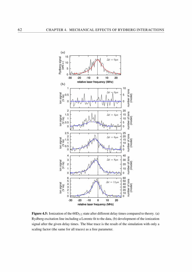
62 CHAPTER 4. MECHANICAL EFFECTS OF RYDBERG INTERACTIONS
(a)
∆t = 0µs
0
5
10
15
-30 -20 -10 0 10 20
Ryd
be
rg s
ign
al
(arb
.u.)
relative laser frequency (MHz)
-30 -20 -10 0 10 20
relative laser frequency (MHz)(b)
∆t = 0µs
0
0.5
1
ion
sig
na
l(V
ns)
0
5
10
nu
mb
er
of
ion
s(m
od
el)
∆t = 4µs
0
0.5
1
1.5
2
ion
sig
na
l(V
ns)
0
5
10
15
20
nu
mb
er
of
ion
s(m
od
el)
∆t = 6µs
0
0.5
11.5
2
2.5
ion
sig
na
l(V
ns)
0
5
1015
20
25
nu
mb
er
of
ion
s(m
od
el)
∆t = 8µs
0
1
2
3
4
ion
sig
na
l(V
ns)
0
10
20
30
40
nu
mb
er
of
ion
s(m
od
el)
∆t = 11µs
0123456
-30 -20 -10 0 10 20
ion
sig
na
l(V
ns)
relative laser frequency (MHz)
-30 -20 -10 0 10 20
0102030405060
nu
mb
er
of
ion
s(m
od
el)
relative laser frequency (MHz)
Figure 4.5: Ionization of the 60D5/2 state after different delay times compared to theory. (a)
Rydberg excitation line including a Lorentz fit to the data, (b) development of the ionization
signal after the given delay times. The blue trace is the result of the simulation with only a
scaling factor (the same for all traces) as a free parameter.
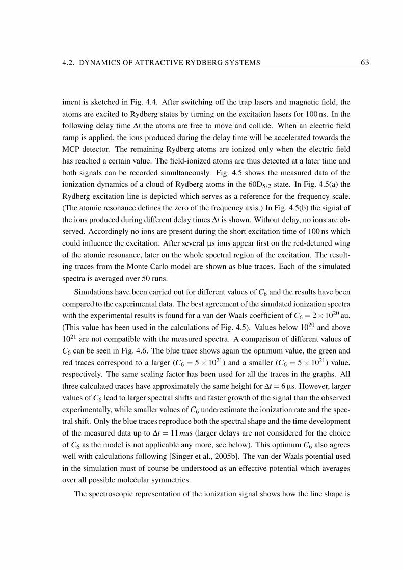
4.2. DYNAMICS OF ATTRACTIVE RYDBERG SYSTEMS 63
iment is sketched in Fig. 4.4. After switching off the trap lasers and magnetic field, the
atoms are excited to Rydberg states by turning on the excitation lasers for 100 ns. In the
following delay time ∆t the atoms are free to move and collide. When an electric field
ramp is applied, the ions produced during the delay time will be accelerated towards the
MCP detector. The remaining Rydberg atoms are ionized only when the electric field
has reached a certain value. The field-ionized atoms are thus detected at a later time and
both signals can be recorded simultaneously. Fig. 4.5 shows the measured data of the
ionization dynamics of a cloud of Rydberg atoms in the 60D5/2 state. In Fig. 4.5(a) the
Rydberg excitation line is depicted which serves as a reference for the frequency scale.
(The atomic resonance defines the zero of the frequency axis.) In Fig. 4.5(b) the signal of
the ions produced during different delay times ∆t is shown. Without delay, no ions are ob-
served. Accordingly no ions are present during the short excitation time of 100 ns which
could influence the excitation. After several µs ions appear first on the red-detuned wing
of the atomic resonance, later on the whole spectral region of the excitation. The result-
ing traces from the Monte Carlo model are shown as blue traces. Each of the simulated
spectra is averaged over 50 runs.
Simulations have been carried out for different values of C6 and the results have been
compared to the experimental data. The best agreement of the simulated ionization spectra
with the experimental results is found for a van der Waals coefficient of C6 = 2×10²⁰ au.
(This value has been used in the calculations of Fig. 4.5). Values below 1020 and above
1021 are not compatible with the measured spectra. A comparison of different values of
C6 can be seen in Fig. 4.6. The blue trace shows again the optimum value, the green and
red traces correspond to a larger (C6 = 5× 10²¹) and a smaller (C6 = 5× 10²¹) value,
respectively. The same scaling factor has been used for all the traces in the graphs. All
three calculated traces have approximately the same height for ∆t = 6µs. However, larger
values of C6 lead to larger spectral shifts and faster growth of the signal than the observed
experimentally, while smaller values of C6 underestimate the ionization rate and the spec-
tral shift. Only the blue traces reproduce both the spectral shape and the time development
of the measured data up to ∆t = 11mus (larger delays are not considered for the choice
of C6 as the model is not applicable any more, see below). This optimum C6 also agrees
well with calculations following [Singer et al., 2005b]. The van der Waals potential used
in the simulation must of course be understood as an effective potential which averages
over all possible molecular symmetries.
The spectroscopic representation of the ionization signal shows how the line shape is
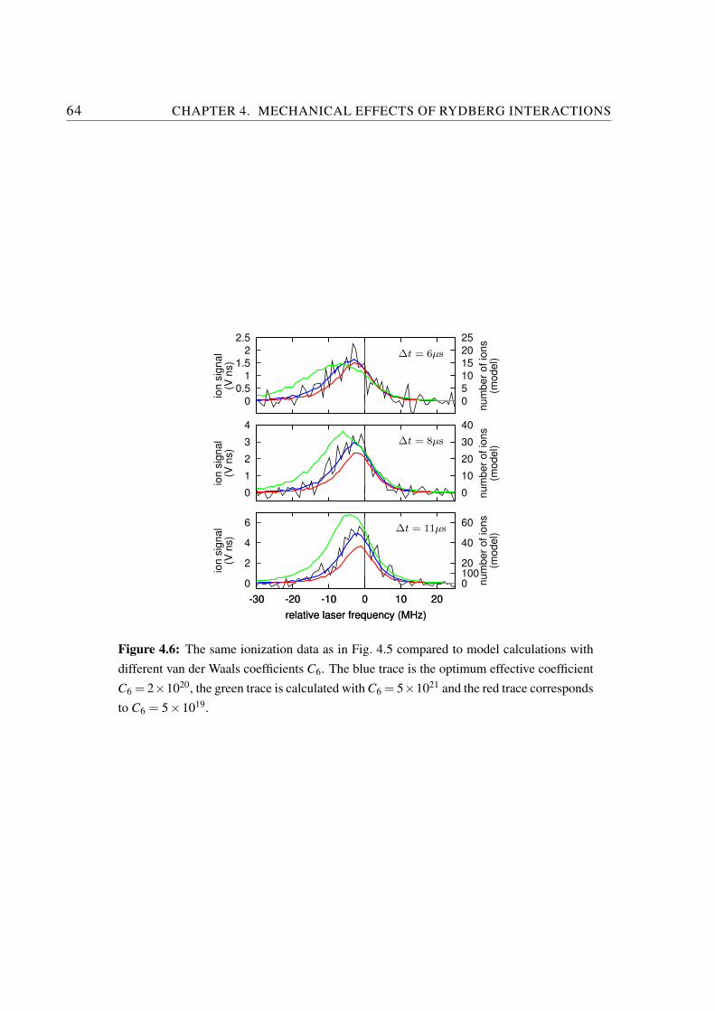
64 CHAPTER 4. MECHANICAL EFFECTS OF RYDBERG INTERACTIONS
∆t = 6µs
0
0.5
11.5
2
2.5
ion s
ignal
(V n
s)
0
5
1015
20
25
num
ber
of io
ns
(model)
∆t = 8µs
0
1
2
3
4
ion s
ignal
(V n
s)
0
10
20
30
40
num
ber
of io
ns
(model)
∆t = 11µs
0
2
4
6
-30 -20 -10 0 10 20
ion s
ignal
(V n
s)
relative laser frequency (MHz)
-30 -20 -10 0 10 20
010020
40
60
num
ber
of io
ns
(model)
relative laser frequency (MHz)
Figure 4.6: The same ionization data as in Fig. 4.5 compared to model calculations with
different van der Waals coefficients C6. The blue trace is the optimum effective coefficient
C6 = 2×10²⁰, the green trace is calculated withC6 = 5×10²¹ and the red trace corresponds
to C6 = 5×10¹⁹.
4.2. DYNAMICS OF ATTRACTIVE RYDBERG SYSTEMS 65
0
0.1
0.2
0.3
fraction o
f io
niz
ed a
tom
s
measurement
0
0.05
0.1
0 2 4 6 8 10 12 14
interaction time ∆t (µs)
model
Figure 4.7: Time dependence of the ionization signal at different excitation laser detunings.
The upper graph shows the measured data, the lower graph the corresponding simulation.
The three laser detunings are: 0 MHz (black, solid), −6 MHz (red, dotted), +6 MHz (blue,
dashed). The relative ionization rates of the different detunings are well reproduced by
the model. For long delay times (∆t > 11µs) the model is not applicable any more and
underestimates the ion production.
reproduced by the simulation. But one can still gain some more insight in the system by
investigating the time development of the measured signal and the model at fixed detun-
ings. In Fig. 4.7 the time development is plotted for three different detunings, 0MHz,
−6MHz (red-detuned), and +6MHz (blue-detuned). The upper graph shows the mea-
sured data, the lower graph displays the results of the simulation. The error bars at the
measured data points represent the standard deviation of fluctuations in the signal. Due to
experimental uncertainties, the fraction of ionized atoms is subject to a systematic error
of a factor of two. The model predicts a threshold for the ion production at around 3-4 µs,
which is also observed in the experiment. The development of the ionization signal at
different detunings relative to each other also shows a similar behavior in model and ex-
periment. At −6 MHz (red detuning), the ionization rate is comparable to the one at zero
detuning. At +6 MHz (blue detuning) the rate is significantly lower.
The model described above will describe the dynamics system only as long as cold
Rydberg–Rydberg collisions are the main source of ionization. When the density of ions
becomes so large that electrons are trapped in the effective potential formed by the ion
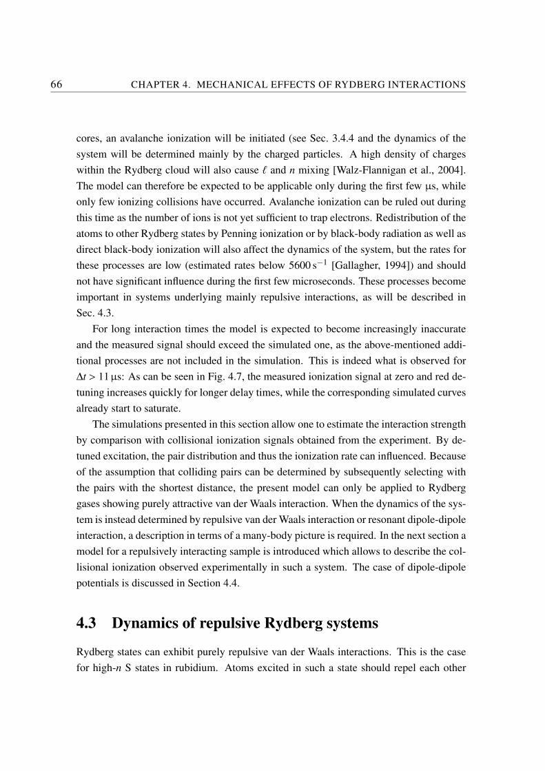
66 CHAPTER 4. MECHANICAL EFFECTS OF RYDBERG INTERACTIONS
cores, an avalanche ionization will be initiated (see Sec. 3.4.4 and the dynamics of the
system will be determined mainly by the charged particles. A high density of charges
within the Rydberg cloud will also cause ℓ and n mixing [Walz-Flannigan et al., 2004].
The model can therefore be expected to be applicable only during the first few µs, while
only few ionizing collisions have occurred. Avalanche ionization can be ruled out during
this time as the number of ions is not yet sufficient to trap electrons. Redistribution of the
atoms to other Rydberg states by Penning ionization or by black-body radiation as well as
direct black-body ionization will also affect the dynamics of the system, but the rates for
these processes are low (estimated rates below 5600 s−1 [Gallagher, 1994]) and should
not have significant influence during the first few microseconds. These processes become
important in systems underlying mainly repulsive interactions, as will be described in
Sec. 4.3.
For long interaction times the model is expected to become increasingly inaccurate
and the measured signal should exceed the simulated one, as the above-mentioned addi-
tional processes are not included in the simulation. This is indeed what is observed for
∆t > 11µs: As can be seen in Fig. 4.7, the measured ionization signal at zero and red de-
tuning increases quickly for longer delay times, while the corresponding simulated curves
already start to saturate.
The simulations presented in this section allow one to estimate the interaction strength
by comparison with collisional ionization signals obtained from the experiment. By de-
tuned excitation, the pair distribution and thus the ionization rate can influenced. Because
of the assumption that colliding pairs can be determined by subsequently selecting with
the pairs with the shortest distance, the present model can only be applied to Rydberg
gases showing purely attractive van der Waals interaction. When the dynamics of the sys-
tem is instead determined by repulsive van der Waals interaction or resonant dipole-dipole
interaction, a description in terms of a many-body picture is required. In the next section a
model for a repulsively interacting sample is introduced which allows to describe the col-
lisional ionization observed experimentally in such a system. The case of dipole-dipole
potentials is discussed in Section 4.4.
4.3 Dynamics of repulsive Rydberg systems
Rydberg states can exhibit purely repulsive van der Waals interactions. This is the case
for high-n S states in rubidium. Atoms excited in such a state should repel each other
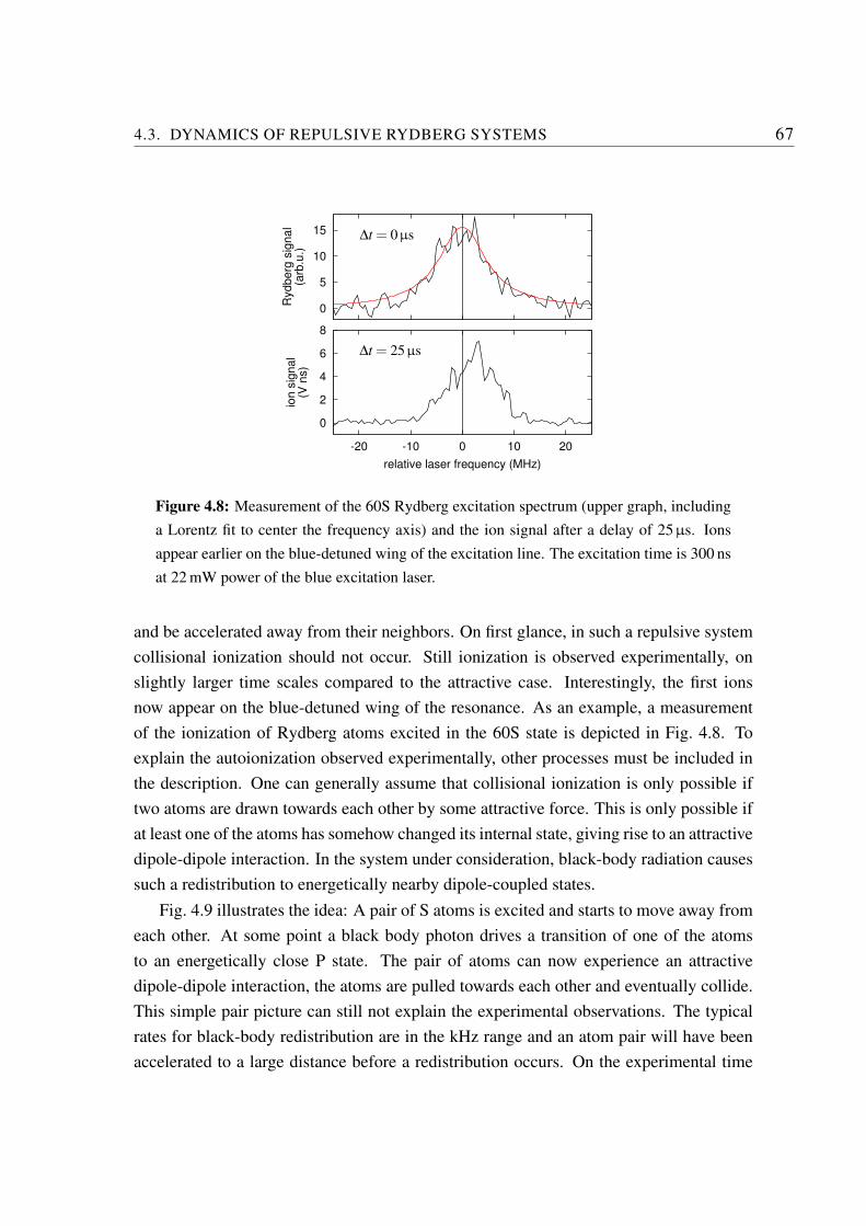
4.3. DYNAMICS OF REPULSIVE RYDBERG SYSTEMS 67
0
5
10
15
Rydberg
sig
nal
(arb
.u.)
0
2
4
6
8
-20 -10 0 10 20
ion s
ignal
(V n
s)
relative laser frequency (MHz)
∆t = 0µs
∆t = 25µs
Figure 4.8: Measurement of the 60S Rydberg excitation spectrum (upper graph, including
a Lorentz fit to center the frequency axis) and the ion signal after a delay of 25µs. Ions
appear earlier on the blue-detuned wing of the excitation line. The excitation time is 300 ns
at 22 mW power of the blue excitation laser.
and be accelerated away from their neighbors. On first glance, in such a repulsive system
collisional ionization should not occur. Still ionization is observed experimentally, on
slightly larger time scales compared to the attractive case. Interestingly, the first ions
now appear on the blue-detuned wing of the resonance. As an example, a measurement
of the ionization of Rydberg atoms excited in the 60S state is depicted in Fig. 4.8. To
explain the autoionization observed experimentally, other processes must be included in
the description. One can generally assume that collisional ionization is only possible if
two atoms are drawn towards each other by some attractive force. This is only possible if
at least one of the atoms has somehow changed its internal state, giving rise to an attractive
dipole-dipole interaction. In the system under consideration, black-body radiation causes
such a redistribution to energetically nearby dipole-coupled states.
Fig. 4.9 illustrates the idea: A pair of S atoms is excited and starts to move away from
each other. At some point a black body photon drives a transition of one of the atoms
to an energetically close P state. The pair of atoms can now experience an attractive
dipole-dipole interaction, the atoms are pulled towards each other and eventually collide.
This simple pair picture can still not explain the experimental observations. The typical
rates for black-body redistribution are in the kHz range and an atom pair will have been
accelerated to a large distance before a redistribution occurs. On the experimental time
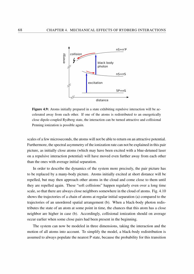
68 CHAPTER 4. MECHANICAL EFFECTS OF RYDBERG INTERACTIONS
Figure 4.9: Atoms initially prepared in a state exhibiting repulsive interaction will be ac-
celerated away from each other. If one of the atoms is redistributed to an energetically
close dipole-coupled Rydberg state, the interaction can be turned attractive and collisional
Penning ionization is possible again.
scales of a few microseconds, the atoms will not be able to return on an attractive potential.
Furthermore, the spectral asymmetry of the ionization rate can not be explained in this pair
picture, as initially close atoms (which may have been excited with a blue-detuned laser
on a repulsive interaction potential) will have moved even further away from each other
than the ones with average initial separation.
In order to describe the dynamics of the system more precisely, the pair picture has
to be replaced by a many-body picture. Atoms initially excited at short distance will be
repelled, but may then approach other atoms in the cloud and come close to them until
they are repelled again. These “soft collisions” happen regularly even over a long time
scale, so that there are always close neighbors somewhere in the cloud of atoms. Fig. 4.10
shows the trajectories of a chain of atoms at regular initial separation (a) compared to the
trajectories of an unordered spatial arrangement (b). When a black-body photon redis-
tributes the state of an atom at some point in time, the chances that this atom has a close
neighbor are higher in case (b). Accordingly, collisional ionization should on average
occur earlier when some close pairs had been present in the beginning.
The system can now be modeled in three dimensions, taking the interaction and the
motion of all atoms into account. To simplify the model, a black-body redistribution is
assumed to always populate the nearest P state, because the probability for this transition
4.3. DYNAMICS OF REPULSIVE RYDBERG SYSTEMS 69
40
20
0
-20
-40
0 5 10 15 20 25 30
po
sitio
n (
µm
)
time (µs)
40
20
0
-20
-40
0 5 10 15 20 25 30
time (µs)
Figure 4.10: A one-dimensional model to visualize the dynamics of repulsive multi-
particle systems. (a) In a regularly spaced chain of atoms a slight repulsion of the atoms is
visible, and the distances between neighboring atoms stays large. (b) If some close pairs
exist in the beginning, these atoms will be repelled more quickly. The faster atoms will
always come close to other particles and during a long timescale there will always be close
pairs somewhere in the ensemble.
is largest. Each of the atoms can thus be in one of three different states, the state of atom
i being denoted by si:
si =
0 ground state
1 initial Rydberg state (S)
2 redistributed Rydberg state (P)
(4.9)
The classical equations of motion for N atoms based on the interatomic interaction po-
tentials can be written as a system of N coupled differential equations. The force acting
on atom i is assumed to be the sum of the forces induced by the interaction with all other
atoms j 6= i, each force given by the gradient of the pair interaction potential. For atom i,
the corresponding equation of motion reads
∑j 6=i
∇Vi j(~r j−~ri) = mRbd2~ri
dt2, (4.10)
where the potential depends on the state of the atoms i and j. If both atoms are in the
initial S state, the interaction is repulsive and of van der Waals type. If one atom is in the
initial state, the other one in a redistributed state, the interaction is of dipole-dipole type.
Interactions of two redistributed atoms are neglected, as the model should only simulate
70 CHAPTER 4. MECHANICAL EFFECTS OF RYDBERG INTERACTIONS
the initial ion production while most atoms are still in their initial states. Explicitly, the
potential Vi j is given by (in atomic units):
Vi j(~r) =
− C6
|~r|6 for si = 1∧ s j = 1
~µi~µ j
|~r|3 −3(~µi~r)(~µ j~r)
|~r|5 for (si = 1∧ s j = 2)∨ (si = 2∧ s j = 1)
0 otherwise
(4.11)
The orientation of the dipole moments ~µi is chosen randomly, with equal absolute values.
The dipole moments are connected to an effective C3 coefficient as |~µi|2 = µ2e f f = C
e f f3 .
This value Ce f f3 is used as a variable parameter in the model. The equations of motion
are now solved by numerical integration. In order to reduce the calculation time, a ded-
icated algorithm adapts the integration stepsize automatically and individually for each
of the particles. The number of integration steps per time interval is derived from the
current velocity of the particle. For slowly moving atoms the position in phase space is
updated in larger time intervals while for fast atoms position and velocity are recalculated
at each integration step. The shortest integration step possible in the calculation is 1 ns, a
sufficiently short time to resolve even fast motion prior to a collision. As most atoms in
the simulation are not accelerated much during the first few microseconds, the adaptive
stepsize technique saves a large amount of calculation time.
Whenever the distance between two atoms i and j becomes less than 4n2a0, these
atoms are assumed to collide and undergo Penning ionization [Robicheaux, 2005, Olson,
1979]. The products of this collision are not considered in the model, and the states of the
two atoms are simply set to zero after a collision, si = s j = 0. The internal state of the
atoms can be influenced during their motion by different processes, each expressed as a
rate Γ, yielding a probability of Γ∆t for this process to happen to a specific atom during
an integration time step ∆t. For each atom, each time step and each redistribution process,
a random number is generated to decide whether this process happens. The following
processes and rates are incorporated in the model:
1. Black-body-induced redistribution to other Rydberg states, Γbb. This process will
mainly lead to nearby states, because of the higher transition matrix elements. The
corresponding rates are calculated following [Gallagher, 1994] and listed in Ta-
ble 4.1. This process changes the state of an atom i from si = 1 to si = 2.
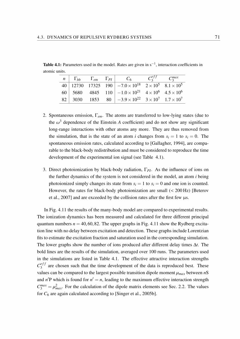
4.3. DYNAMICS OF REPULSIVE RYDBERG SYSTEMS 71
Table 4.1: Parameters used in the model. Rates are given in s−1, interaction coefficients in
atomic units.
n Γbb Γem ΓPI C6 Ce f f3 Cmax
3
40 12730 17325 190 −7.0×10¹⁸ 2×10⁵ 8.1×10⁵
60 5680 4845 110 −1.0×10²¹ 4×10⁶ 4.5×10⁶
82 3030 1853 80 −3.9×10²² 3×10⁷ 1.7×10⁷
2. Spontaneous emission, Γem. The atoms are transferred to low-lying states (due to
the ω3 dependence of the Einstein A coefficient) and do not show any significant
long-range interactions with other atoms any more. They are thus removed from
the simulation, that is the state of an atom i changes from si = 1 to si = 0. The
spontaneous emission rates, calculated according to [Gallagher, 1994], are compa-
rable to the black-body redistribution and must be considered to reproduce the time
development of the experimental ion signal (see Table 4.1).
3. Direct photoionization by black-body radiation, ΓPI . As the influence of ions on
the further dynamics of the system is not considered in the model, an atom i being
photoionized simply changes its state from si = 1 to si = 0 and one ion is counted.
However, the rates for black-body photoionization are small (< 200 Hz) [Beterov
et al., 2007] and are exceeded by the collision rates after the first few µs.
In Fig. 4.11 the results of the many-body model are compared to experimental results.
The ionization dynamics has been measured and calculated for three different principal
quantum numbers n = 40,60,82. The upper graphs in Fig. 4.11 show the Rydberg excita-
tion line with no delay between excitation and detection. These graphs include Lorentzian
fits to estimate the excitation fraction and saturation used in the corresponding simulation.
The lower graphs show the number of ions produced after different delay times ∆t. The
bold lines are the results of the simulation, averaged over 100 runs. The parameters used
in the simulations are listed in Table 4.1. The effective attractive interaction strengths
Ce f f3 are chosen such that the time development of the data is reproduced best. These
values can be compared to the largest possible transition dipole moment µmax between nS
and n′P which is found for n′ = n, leading to the maximum effective interaction strength
Cmax3 = µ2
max. For the calculation of the dipole matrix elements see Sec. 2.2. The values
for C6 are again calculated according to [Singer et al., 2005b].
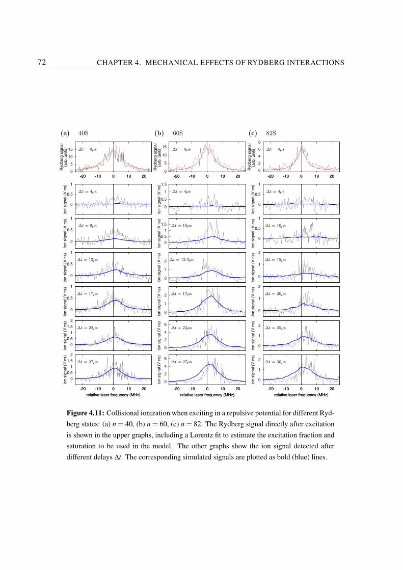
72 CHAPTER 4. MECHANICAL EFFECTS OF RYDBERG INTERACTIONS
(a) 40S (b) 60S (c) 82S
∆t = 0µs
0
5
10
15
-20 -10 0 10 20
Rydberg
sig
nal
(arb
. units)
-20 -10 0 10 20
∆t = 0µs
0
5
10
15
-20 -10 0 10 20
Rydberg
sig
nal
(arb
. units)
-20 -10 0 10 20
∆t = 0µs
0
2
4
6
8
-20 -10 0 10 20
Rydberg
sig
nal
(arb
. units)
-20 -10 0 10 20
∆t = 4µs
0
0.5
1
ion s
ignal (V
ns)
∆t = 4µs
0
0.5
1
1.5
ion s
ignal (V
ns)
∆t = 4µs
0
0.5
1
ion s
ignal (V
ns)
∆t = 9µs
0
0.5
1
ion s
ignal (V
ns)
∆t = 10µs
0
0.5
1
1.5
ion s
ignal (V
ns)
∆t = 10µs
0
0.5
1
ion s
ignal (V
ns)
∆t = 13µs
0
0.5
1
ion s
ignal (V
ns)
∆t = 12.5µs
0
1
2
ion s
ignal (V
ns)
∆t = 15µs
0
1
2io
n s
ignal (V
ns)
∆t = 17µs
0
0.5
1
ion s
ignal (V
ns)
∆t = 17µs
0
1
2
ion s
ignal (V
ns)
∆t = 20µs
0
1
2
ion s
ignal (V
ns)
∆t = 22µs
0
0.5
1
1.5
2
ion s
ignal (V
ns)
∆t = 23µs
0
2
4
6
ion s
ignal (V
ns)
∆t = 25µs
0
1
2
ion s
ignal (V
ns)
∆t = 27µs
0
0.5
1
1.5
2
-20 -10 0 10 20
ion s
ignal (V
ns)
relative laser frequency (MHz)
-20 -10 0 10 20
relative laser frequency (MHz)
∆t = 27µs
0
2
4
6
-20 -10 0 10 20
ion s
ignal (V
ns)
relative laser frequency (MHz)
-20 -10 0 10 20
relative laser frequency (MHz)
∆t = 30µs
0
1
2
-20 -10 0 10 20
ion s
ignal (V
ns)
relative laser frequency (MHz)
-20 -10 0 10 20
relative laser frequency (MHz)
Figure 4.11: Collisional ionization when exciting in a repulsive potential for different Ryd-
berg states: (a) n = 40, (b) n = 60, (c) n = 82. The Rydberg signal directly after excitation
is shown in the upper graphs, including a Lorentz fit to estimate the excitation fraction and
saturation to be used in the model. The other graphs show the ion signal detected after
different delays ∆t. The corresponding simulated signals are plotted as bold (blue) lines.
4.3. DYNAMICS OF REPULSIVE RYDBERG SYSTEMS 73
The qualitative behavior of the ionization dynamics is very well reproduced: The
maximum initial ionization rate is found on the blue-detuned side of the atomic resonance.
This spectral shift increases towards higher n, as the interaction-induced variation in the
pair distance distribution becomes more distinct. For n = 40, no significant asymmetry
can be seen in the ionization signal, while for n = 82 the spectral shift is clearly visible.
The simulated curves for the ion production have been scaled to the experimental data.
For all traces belonging to the same principal quantum number n, the same scaling factor
has been used. Satisfactory overlap of all the curves could only be achieved when using
different scaling factors for different principal quantum numbers. This is not surprising
considering that there are several effects which have not been considered in the model.
1. Secondary effects of the collision products, such as local electric fields caused by
the ions, state-changing collisions [Walz-Flannigan et al., 2004], and avalanche
ionization effects are neglected.
2. Additional redistribution by superradiant effects have not been included. Superradi-
ance has been found to play a role in dense Rydberg samples [Wang et al., 2007,Day
et al., 2008, Gounand et al., 1979].
3. The interaction potentials at short distance are not exactly known. Furthermore,
admixture of other states when two atoms are in close vicinity to each other is not
considered.
4. Another distance-dependent ionization process is the resonant coupling of few-
body states to the ionization continuum. As long as only direct coupling of pair
states is considered, this process is not significant (see Sec. 3.4.3). But taking into
account a larger number of intermediate pair states or even many-particle states may
result in higher ionization rates [Tanner et al., 2008].
A considerable number of atoms may therefore experience a mixing of states in addition
to the black-body-induced redistribution, especially for high principal quantum numbers,
where the interactions are stronger. This implies that the ion production should be sys-
tematically underestimated as n is increased, and accordingly the Ce f f3 should be over-
estimated. This is in fact what is found from the comparison of the simulated ion signal
to to measurement: For the 40S state the simulated ionization fraction at ∆t = 30µs is
3.0%, which corresponds reasonably well to the experimental estimate of 4–8%. As n
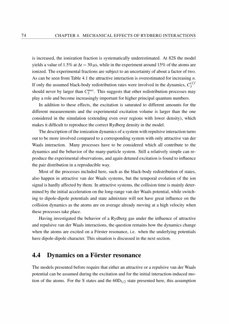
74 CHAPTER 4. MECHANICAL EFFECTS OF RYDBERG INTERACTIONS
is increased, the ionization fraction is systematically underestimated. At 82S the model
yields a value of 1.5% at ∆t = 30µs, while in the experiment around 15% of the atoms are
ionized. The experimental fractions are subject to an uncertainty of about a factor of two.
As can be seen from Table 4.1 the attractive interaction is overestimated for increasing n.
If only the assumed black-body redistribution rates were involved in the dynamics, Ce f f3
should never by larger than Cmax3 . This suggests that other redistribution processes may
play a role and become increasingly important for higher principal quantum numbers.
In addition to these effects, the excitation is saturated to different amounts for the
different measurements and the experimental excitation volume is larger than the one
considered in the simulation (extending even over regions with lower density), which
makes it difficult to reproduce the correct Rydberg density in the model.
The description of the ionization dynamics of a system with repulsive interaction turns
out to be more involved compared to a corresponding system with only attractive van der
Waals interaction. Many processes have to be considered which all contribute to the
dynamics and the behavior of the many-particle system. Still a relatively simple can re-
produce the experimental observations, and again detuned excitation is found to influence
the pair distribution in a reproducible way.
Most of the processes included here, such as the black-body redistribution of states,
also happen in attractive van der Waals systems, but the temporal evolution of the ion
signal is hardly affected by them. In attractive systems, the collision time is mainly deter-
mined by the initial acceleration on the long-range van der Waals potential, while switch-
ing to dipole-dipole potentials and state admixture will not have great influence on the
collision dynamics as the atoms are on average already moving at a high velocity when
these processes take place.
Having investigated the behavior of a Rydberg gas under the influence of attractive
and repulsive van der Waals interactions, the question remains how the dynamics change
when the atoms are excited on a Forster resonance, i.e. when the underlying potentials
have dipole-dipole character. This situation is discussed in the next section.
4.4 Dynamics on a Forster resonance
The models presented before require that either an attractive or a repulsive van der Waals
potential can be assumed during the excitation and for the initial interaction-induced mo-
tion of the atoms. For the S states and the 60D5/2 state presented here, this assumption
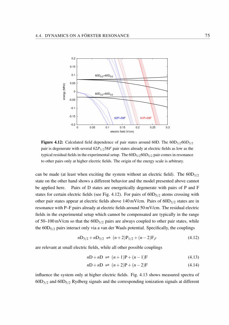
4.4. DYNAMICS ON A FORSTER RESONANCE 75
-0.2
-0.15
-0.1
-0.05
0
0.05
0.1
0.15
0.2
0 0.05 0.1 0.15 0.2 0.25 0.3
en
erg
y (
MH
z)
electric field (V/cm)
61P+59F62P+58F
60D5/2+60D5/2
60D3/2+60D3/2
Figure 4.12: Calculated field dependence of pair states around 60D. The 60D3/260D3/2
pair is degenerate with several 62P1/258F pair states already at electric fields as low as the
typical residual fields in the experimental setup. The 60D5/260D5/2 pair comes in resonance
to other pairs only at higher electric fields. The origin of the energy scale is arbitrary.
can be made (at least when exciting the system without an electric field). The 60D3/2
state on the other hand shows a different behavior and the model presented above cannot
be applied here. Pairs of D states are energetically degenerate with pairs of P and F
states for certain electric fields (see Fig. 4.12). For pairs of 60D5/2 atoms crossing with
other pair states appear at electric fields above 140 mV/cm. Pairs of 60D3/2 states are in
resonance with P–F pairs already at electric fields around 50 mV/cm. The residual electric
fields in the experimental setup which cannot be compensated are typically in the range
of 50–100 mV/cm so that the 60D3/2 pairs are always coupled to other pair states, while
the 60D5/2 pairs interact only via a van der Waals potential. Specifically, the couplings
nD3/2 +nD3/2 (n+2)P1/2 +(n−2)FJ′ (4.12)
are relevant at small electric fields, while all other possible couplings
nD+nD (n+1)P+(n−1)F (4.13)
nD+nD (n+2)P+(n−2)F (4.14)
influence the system only at higher electric fields. Fig. 4.13 shows measured spectra of
60D3/2 and 60D5/2 Rydberg signals and the corresponding ionization signals at different
76 CHAPTER 4. MECHANICAL EFFECTS OF RYDBERG INTERACTIONS
∆t = 6µs
0
2
4
6
8
10
12
14
-70 -60 -50 -40 -30 -20 -10 0 10 20
de
tecto
r sig
na
l (V
ns)
∆t = 8µs
0
2
4
6
8
10
12
14
-70 -60 -50 -40 -30 -20 -10 0 10 20
de
tecto
r sig
na
l (V
ns)
∆t = 11µs
0
2
4
6
8
10
12
14
-70 -60 -50 -40 -30 -20 -10 0 10 20
de
tecto
r sig
na
l (V
ns)
relative laser frequency (MHz)
Figure 4.13: Collisional ionization of the 60D state at different delay times after the exci-
tation. The black trace is the Rydberg signal measured at the given delay, the red trace is
the signal of the ions produced by collisions at the same time. The ion signal is scaled with
a factor of 5 with respect to the Rydberg signal for better visibility. The 60D5/2 component
shows the typical spectral shift of the ionization signal, while the 60D3/2 component ionizes
symmetrically to the atomic resonance. Furthermore, the ionization rate of the 60D3/2 state
is clearly smaller than that of the 60D5/2 state. The differences are caused by the fact that
the 60D5/2 pairs interact via purely attractive van der Waals potentials, while the 60D3/2
pairs are subject to a more complex dipole-dipole interaction.
4.5. SHAPING THE PAIR DISTRIBUTION 77
delay times. The maximum ionization of the 60D5/2 states is red-shifted with respect to
the center of the excitation line, as described before. The 60D3/2 state ionization is sym-
metric to the Rydberg line and its ionization rate is smaller than the one of 60D5/2. Due
to the coupling to other pair states, the interaction potentials differ from a pure van der
Waals shape. Depending on the energetic distance to the resonance, the potentials acquire
dipole-dipole character and exhibit both attractive and repulsive branches. Furthermore,
a redistribution of Rydberg states to the involved P and F levels takes place (see model
calculations in Sec. 5.5). The pair distribution after the excitation of the 60D3/2 state can
therefore not be derived from a simple attractive van der Waals potential. The differences
in the pair distribution for red and blue detuning should be expected to be less pronounced
because the involved potentials are not purely attractive. Instead, the dipole-dipole inter-
action suggest a more symmetric configuration of attractive and repulsive potentials and
may even be able to stabilize the system with regard to collisions.
The Monte Carlo model presented before is well suited to simulate interacting Ryd-
berg systems as long as the van der Waals interaction determines the dynamics. In the
case of resonant dipole-dipole interaction, however, both the excitation and the evolution
of the system must be described differently: It has been shown in Sec. 3.3 that for atoms
interacting with a 1/R3-dependent potential, the restriction to the nearest Rydberg neigh-
bor when modeling the excitation is not justified any more. For the simulation of the
atomic motion it may further be necessary to consider the system as a superposition of
many-body states instead of pairwise interacting atoms in well-defined states. A quantum
mechanical few-body model as the one presented in Sec. 5.3.1 can be more appropriate
in this case, provided that the excitation and atomic motion are included. The motion in
chain of atoms described by many-body states is investigated in [Ates et al., 2008]. A
similar model may be developed for the case of an unordered gas prepared by detuned
excitation.
4.5 Shaping the pair distribution
As investigated in the previous sections, the pair distribution of an ultracold Rydberg gas
can be influenced by detuning the excitation laser from resonance. This induces spatial
correlations in the gas in a controllable way. Given a system with underlying repulsive van
der Waals Potentials, spatial correlations in the cloud can even develop automatically after
some time, because the particles start to move according to the interatomic interaction
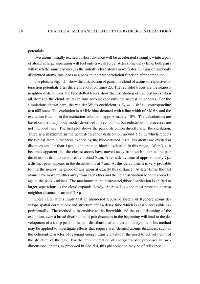
78 CHAPTER 4. MECHANICAL EFFECTS OF RYDBERG INTERACTIONS
potentials.
Two atoms initially excited at short distance will be accelerated strongly, while a pair
of atoms at large separation will feel only a weak force. After some delay time, both pairs
will reach the same distance, as the initially close atoms move faster. In a gas of randomly
distributed atoms, this leads to a peak in the pair correlation function after some time.
The plots in Fig. 4.14 show the distribution of pairs in a cloud of atoms on repulsive in-
teraction potentials after different evolution times ∆t. The red solid traces are the nearest-
neighbor distributions, the blue dotted traces show the distribution of pair distances when
all atoms in the cloud are taken into account (not only the nearest neighbors). For the
simulations shown here, the van der Waals coefficient is C6 = −1021 au, corresponding
to a 60S state. The excitation is 6 MHz blue-detuned with a line width of 8MHz, and the
excitation fraction in the excitation volume is approximately 10%. The calculations are
based on the many-body model described in Section 4.3, but redistribution processes are
not included here. The first plot shows the pair distribution directly after the excitation.
There is a maximum in the nearest-neighbor distribution around 5.5µm which reflects
the typical atomic distances excited by the blue-detuned laser. No atoms are excited at
distances smaller than 4µm, as interaction blocks excitation in this range. After 3µs it
becomes apparent that the closest atoms have moved away from each other, as the pair
distributions drop to zero already around 5µm. After a delay time of approximately 7µs
a distinct peak appears in the distributions at 7µm. At this delay time it is very probable
to find the nearest neighbor of any atom at exactly this distance. At later times the fast
atoms have moved further away from each other and the pair distribution becomes broader
again, the peak vanishes. The maximum in the nearest-neighbor distribution is shifted to
larger separations as the cloud expands slowly. At ∆t = 14µs the most probable nearest
neighbor distance is around 7.8µm.
These calculations imply that an unordered repulsive system of Rydberg atoms de-
velops spatial correlations and structure after a delay time which is easily accessible ex-
perimentally. The method is insensitive to the linewidth and the exact detuning of the
excitation, even a broad distribution of pair distances in the beginning will lead to the de-
velopment of a sharp peak in the pair distribution after a certain delay time. This method
may be applied to investigate effects that require well-defined atomic distances, such as
the coherent character of resonant energy transfer, without the need to actively control
the structure of the gas. For the implementation of energy transfer processes in one-
dimensional chains, as proposed in Sec. 5.4, this phenomenon may be of relevance.
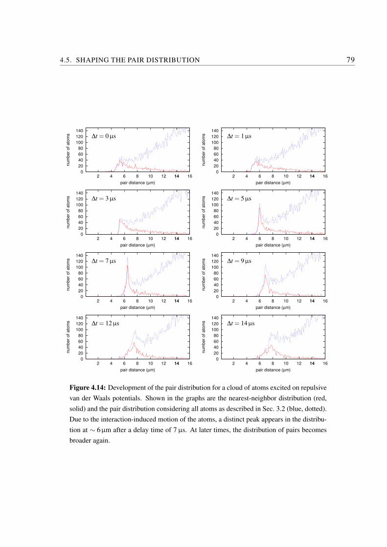
4.5. SHAPING THE PAIR DISTRIBUTION 79
0
20
40
60
80
100
120
140
16141412108642
nu
mb
er
of
ato
ms
pair distance (µm)
∆t = 0µs
0
20
40
60
80
100
120
140
16141412108642
nu
mb
er
of
ato
ms
pair distance (µm)
∆t = 1µs
0
20
40
60
80
100
120
140
16141412108642
nu
mb
er
of
ato
ms
pair distance (µm)
∆t = 3µs
0
20
40
60
80
100
120
140
16141412108642
nu
mb
er
of
ato
ms
pair distance (µm)
∆t = 5µs
0
20
40
60
80
100
120
140
16141412108642
nu
mb
er
of
ato
ms
pair distance (µm)
∆t = 7µs
0
20
40
60
80
100
120
140
16141412108642
nu
mb
er
of
ato
ms
pair distance (µm)
∆t = 9µs
0
20
40
60
80
100
120
140
16141412108642
nu
mb
er
of
ato
ms
pair distance (µm)
∆t = 12µs
0
20
40
60
80
100
120
140
16141412108642
nu
mb
er
of
ato
ms
pair distance (µm)
∆t = 14µs
Figure 4.14: Development of the pair distribution for a cloud of atoms excited on repulsive
van der Waals potentials. Shown in the graphs are the nearest-neighbor distribution (red,
solid) and the pair distribution considering all atoms as described in Sec. 3.2 (blue, dotted).
Due to the interaction-induced motion of the atoms, a distinct peak appears in the distribu-
tion at ∼ 6µm after a delay time of 7 µs. At later times, the distribution of pairs becomes
broader again.
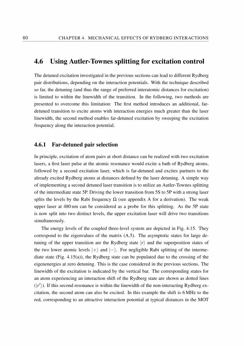
80 CHAPTER 4. MECHANICAL EFFECTS OF RYDBERG INTERACTIONS
4.6 Using Autler-Townes splitting for excitation control
The detuned excitation investigated in the previous sections can lead to different Rydberg
pair distributions, depending on the interaction potentials. With the technique described
so far, the detuning (and thus the range of preferred interatomic distances for excitation)
is limited to within the linewidth of the transition. In the following, two methods are
presented to overcome this limitation: The first method introduces an additional, far-
detuned transition to excite atoms with interaction energies much greater than the laser
linewidth, the second method enables far-detuned excitation by sweeping the excitation
frequency along the interaction potential.
4.6.1 Far-detuned pair selection
In principle, excitation of atom pairs at short distance can be realized with two excitation
lasers, a first laser pulse at the atomic resonance would excite a bath of Rydberg atoms,
followed by a second excitation laser, which is far-detuned and excites partners to the
already excited Rydberg atoms at distances defined by the laser detuning. A simple way
of implementing a second detuned laser transition is to utilize an Autler-Townes splitting
of the intermediate state 5P. Driving the lower transition from 5S to 5P with a strong laser
splits the levels by the Rabi frequency Ω (see appendix A for a derivation). The weak
upper laser at 480 nm can be considered as a probe for this splitting. As the 5P state
is now split into two distinct levels, the upper excitation laser will drive two transitions
simultaneously.
The energy levels of the coupled three-level system are depicted in Fig. 4.15. They
correspond to the eigenvalues of the matrix (A.5). The asymptotic states for large de-
tuning of the upper transition are the Rydberg state |r〉 and the superposition states of
the two lower atomic levels |+〉 and |−〉. For negligible Rabi splitting of the interme-
diate state (Fig. 4.15(a)), the Rydberg state can be populated due to the crossing of the
eigenenergies at zero detuning. This is the case considered in the previous sections. The
linewidth of the excitation is indicated by the vertical bar. The corresponding states for
an atom experiencing an interaction shift of the Rydberg state are shown as dotted lines
(|r′〉). If this second resonance is within the linewidth of the non-interacting Rydberg ex-
citation, the second atom can also be excited. In this example the shift is 6 MHz to the
red, corresponding to an attractive interaction potential at typical distances in the MOT
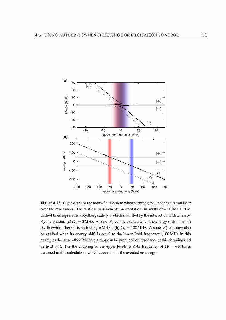
4.6. USING AUTLER-TOWNES SPLITTING FOR EXCITATION CONTROL 81
-30
-20
-10
0
10
20
30
-40 -20 0 20 40
energ
y (
MH
z)
upper laser detuning (MHz)
(a)
-200
-100
0
100
200
-200 -150 -100 -50 0 50 100 150 200
energ
y (
MH
z)
upper laser detuning (MHz)
(b)
|+〉
|+〉
|−〉
|−〉
|r〉
|r〉
|r′〉
|r′〉
Figure 4.15: Eigenstates of the atom–field system when scanning the upper excitation laser
over the resonances. The vertical bars indicate an excitation linewidth of ∼ 10MHz. The
dashed lines represents a Rydberg state |r′〉 which is shifted by the interaction with a nearby
Rydberg atom. (a) Ω1 = 2MHz. A state |r′〉 can be excited when the energy shift is within
the linewidth (here it is shifted by 6 MHz). (b) Ω1 = 100MHz. A state |r′〉 can now also
be excited when its energy shift is equal to the lower Rabi frequency (100 MHz in this
example), because other Rydberg atoms can be produced on resonance at this detuning (red
vertical bar). For the coupling of the upper levels, a Rabi frequency of Ω2 = 4 MHz is
assumed in this calculation, which accounts for the avoided crossings.
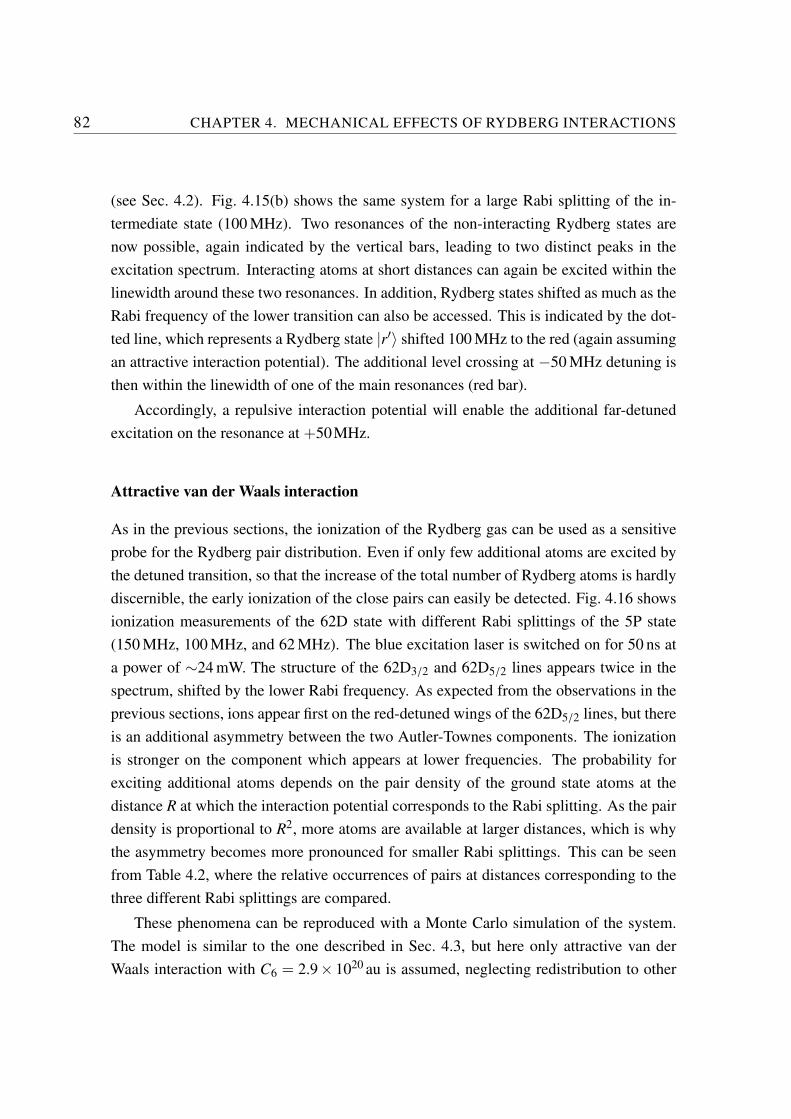
82 CHAPTER 4. MECHANICAL EFFECTS OF RYDBERG INTERACTIONS
(see Sec. 4.2). Fig. 4.15(b) shows the same system for a large Rabi splitting of the in-
termediate state (100 MHz). Two resonances of the non-interacting Rydberg states are
now possible, again indicated by the vertical bars, leading to two distinct peaks in the
excitation spectrum. Interacting atoms at short distances can again be excited within the
linewidth around these two resonances. In addition, Rydberg states shifted as much as the
Rabi frequency of the lower transition can also be accessed. This is indicated by the dot-
ted line, which represents a Rydberg state |r′〉 shifted 100 MHz to the red (again assuming
an attractive interaction potential). The additional level crossing at −50 MHz detuning is
then within the linewidth of one of the main resonances (red bar).
Accordingly, a repulsive interaction potential will enable the additional far-detuned
excitation on the resonance at +50MHz.
Attractive van der Waals interaction
As in the previous sections, the ionization of the Rydberg gas can be used as a sensitive
probe for the Rydberg pair distribution. Even if only few additional atoms are excited by
the detuned transition, so that the increase of the total number of Rydberg atoms is hardly
discernible, the early ionization of the close pairs can easily be detected. Fig. 4.16 shows
ionization measurements of the 62D state with different Rabi splittings of the 5P state
(150 MHz, 100 MHz, and 62 MHz). The blue excitation laser is switched on for 50 ns at
a power of ∼24 mW. The structure of the 62D3/2 and 62D5/2 lines appears twice in the
spectrum, shifted by the lower Rabi frequency. As expected from the observations in the
previous sections, ions appear first on the red-detuned wings of the 62D5/2 lines, but there
is an additional asymmetry between the two Autler-Townes components. The ionization
is stronger on the component which appears at lower frequencies. The probability for
exciting additional atoms depends on the pair density of the ground state atoms at the
distance R at which the interaction potential corresponds to the Rabi splitting. As the pair
density is proportional to R2, more atoms are available at larger distances, which is why
the asymmetry becomes more pronounced for smaller Rabi splittings. This can be seen
from Table 4.2, where the relative occurrences of pairs at distances corresponding to the
three different Rabi splittings are compared.
These phenomena can be reproduced with a Monte Carlo simulation of the system.
The model is similar to the one described in Sec. 4.3, but here only attractive van der
Waals interaction with C6 = 2.9× 10²⁰ au is assumed, neglecting redistribution to other
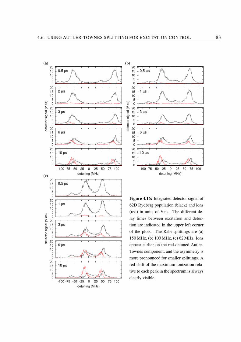
4.6. USING AUTLER-TOWNES SPLITTING FOR EXCITATION CONTROL 83
0
5
10
15
200.5 µs
(a)
0
5
10
15
202 µs
0
5
10
15
203 µs
0
5
10
15
206 µs
0
5
10
15
20
-100 -75 -50 -25 0 25 50 75 100
detuning (MHz)
10 µs
dete
cto
r sig
nal (V
ns)
0
5
10
15
200.5 µs
(c)
0
5
10
15
201 µs
0
5
10
15
203 µs
0
5
10
15
206 µs
0
5
10
15
20
-100 -75 -50 -25 0 25 50 75 100
detuning (MHz)
10 µs
dete
cto
r sig
nal (V
ns)
0
5
10
15
200.5 µs
(b)
0
5
10
15
201 µs
0
5
10
15
203 µs
0
5
10
15
206 µs
0
5
10
15
20
-100 -75 -50 -25 0 25 50 75 100
detuning (MHz)
10 µs
dete
cto
r sig
nal (V
ns)
Figure 4.16: Integrated detector signal of
62D Rydberg population (black) and ions
(red) in units of V ns. The different de-
lay times between excitation and detec-
tion are indicated in the upper left corner
of the plots. The Rabi splittings are (a)
150 MHz, (b) 100 MHz, (c) 62 MHz. Ions
appear earlier on the red-detuned Autler-
Townes component, and the asymmetry is
more pronounced for smaller splittings. A
red-shift of the maximum ionization rela-
tive to each peak in the spectrum is always
clearly visible.
84 CHAPTER 4. MECHANICAL EFFECTS OF RYDBERG INTERACTIONS
0
0.1
0.2
0.3
0µs
(a)
0 0.001 0.002 0.003 0.004 0.005
2µs
0
0.005
0.01
0.015
0.02
4µs
0
0.01
0.02
0.03
0.04
7µs
0 0.01 0.02 0.03 0.04 0.05
-100 -50 0 50 100
detuning (MHz)
10µs
fraction o
f to
tal num
ber
of ato
ms
0
0.1
0.2
0.3
0µs
(c)
0 0.001 0.002 0.003 0.004 0.005
2µs
0
0.005
0.01
0.015
0.02
4µs
0
0.01
0.02
0.03
0.04
7µs
0 0.01 0.02 0.03 0.04 0.05
-100 -50 0 50 100
detuning (MHz)
10µs
fraction o
f to
tal num
ber
of ato
ms
0
0.1
0.2
0.3
0µs
(b)
0 0.001 0.002 0.003 0.004 0.005
2µs
0
0.005
0.01
0.015
0.02
4µs
0
0.01
0.02
0.03
0.04
7µs
0 0.01 0.02 0.03 0.04 0.05
-100 -50 0 50 100
detuning (MHz)
10µs
fraction o
f to
tal num
ber
of ato
ms
Figure 4.17: Simulated Rydberg exci-
tation and ionizing collisions under the
presence of an Autler-Townes splitting
and attractive van der Waals potentials.
The plots show the Rydberg signal (black)
for ∆t = 0µs and the ion signal (red) for
∆t > 0µs. The delay between excitation
and detection is indicated in the corner of
the plots. The signals are given as frac-
tion of the total number of atoms in the
simulation. The splitting is (a) 150 MHz,
(b) 100 MHz, (c) 62 MHz. The vertical
lines correspond to the position of the res-
onances.
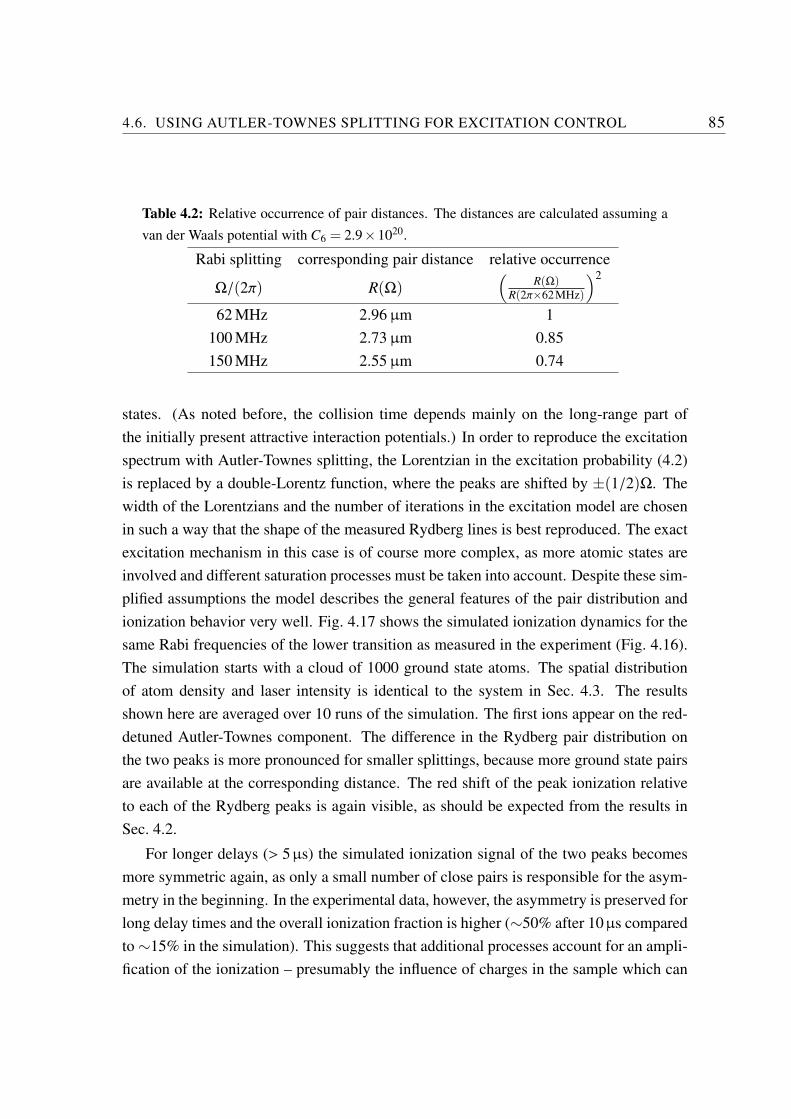
4.6. USING AUTLER-TOWNES SPLITTING FOR EXCITATION CONTROL 85
Table 4.2: Relative occurrence of pair distances. The distances are calculated assuming a
van der Waals potential with C6 = 2.9×10²⁰.
Rabi splitting corresponding pair distance relative occurrence
Ω/(2π) R(Ω)(
R(Ω)R(2π×62MHz)
)2
62 MHz 2.96 µm 1
100 MHz 2.73 µm 0.85
150 MHz 2.55 µm 0.74
states. (As noted before, the collision time depends mainly on the long-range part of
the initially present attractive interaction potentials.) In order to reproduce the excitation
spectrum with Autler-Townes splitting, the Lorentzian in the excitation probability (4.2)
is replaced by a double-Lorentz function, where the peaks are shifted by ±(1/2)Ω. The
width of the Lorentzians and the number of iterations in the excitation model are chosen
in such a way that the shape of the measured Rydberg lines is best reproduced. The exact
excitation mechanism in this case is of course more complex, as more atomic states are
involved and different saturation processes must be taken into account. Despite these sim-
plified assumptions the model describes the general features of the pair distribution and
ionization behavior very well. Fig. 4.17 shows the simulated ionization dynamics for the
same Rabi frequencies of the lower transition as measured in the experiment (Fig. 4.16).
The simulation starts with a cloud of 1000 ground state atoms. The spatial distribution
of atom density and laser intensity is identical to the system in Sec. 4.3. The results
shown here are averaged over 10 runs of the simulation. The first ions appear on the red-
detuned Autler-Townes component. The difference in the Rydberg pair distribution on
the two peaks is more pronounced for smaller splittings, because more ground state pairs
are available at the corresponding distance. The red shift of the peak ionization relative
to each of the Rydberg peaks is again visible, as should be expected from the results in
Sec. 4.2.
For longer delays (> 5µs) the simulated ionization signal of the two peaks becomes
more symmetric again, as only a small number of close pairs is responsible for the asym-
metry in the beginning. In the experimental data, however, the asymmetry is preserved for
long delay times and the overall ionization fraction is higher (∼50% after 10µs compared
to ∼15% in the simulation). This suggests that additional processes account for an ampli-
fication of the ionization – presumably the influence of charges in the sample which can
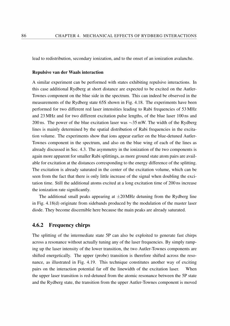
86 CHAPTER 4. MECHANICAL EFFECTS OF RYDBERG INTERACTIONS
lead to redistribution, secondary ionization, and to the onset of an ionization avalanche.
Repulsive van der Waals interaction
A similar experiment can be performed with states exhibiting repulsive interactions. In
this case additional Rydberg at short distance are expected to be excited on the Autler-
Townes component on the blue side in the spectrum. This can indeed be observed in the
measurements of the Rydberg state 65S shown in Fig. 4.18. The experiments have been
performed for two different red laser intensities leading to Rabi frequencies of 53 MHz
and 23 MHz and for two different excitation pulse lengths, of the blue laser 100 ns and
200 ns. The power of the blue excitation laser was ∼35 mW. The width of the Rydberg
lines is mainly determined by the spatial distribution of Rabi frequencies in the excita-
tion volume. The experiments show that ions appear earlier on the blue-detuned Autler-
Townes component in the spectrum, and also on the blue wing of each of the lines as
already discussed in Sec. 4.3. The asymmetry in the ionization of the two components is
again more apparent for smaller Rabi splittings, as more ground state atom pairs are avail-
able for excitation at the distances corresponding to the energy difference of the splitting.
The excitation is already saturated in the center of the excitation volume, which can be
seen from the fact that there is only little increase of the signal when doubling the exci-
tation time. Still the additional atoms excited at a long excitation time of 200 ns increase
the ionization rate significantly.
The additional small peaks appearing at ±20MHz detuning from the Rydberg line
in Fig. 4.18(d) originate from sidebands produced by the modulation of the master laser
diode. They become discernible here because the main peaks are already saturated.
4.6.2 Frequency chirps
The splitting of the intermediate state 5P can also be exploited to generate fast chirps
across a resonance without actually tuning any of the laser frequencies. By simply ramp-
ing up the laser intensity of the lower transition, the two Autler-Townes components are
shifted energetically. The upper (probe) transition is therefore shifted across the reso-
nance, as illustrated in Fig. 4.19. This technique constitutes another way of exciting
pairs on the interaction potential far off the linewidth of the excitation laser. When
the upper laser transition is red-detuned from the atomic resonance between the 5P state
and the Rydberg state, the transition from the upper Autler-Townes component is moved
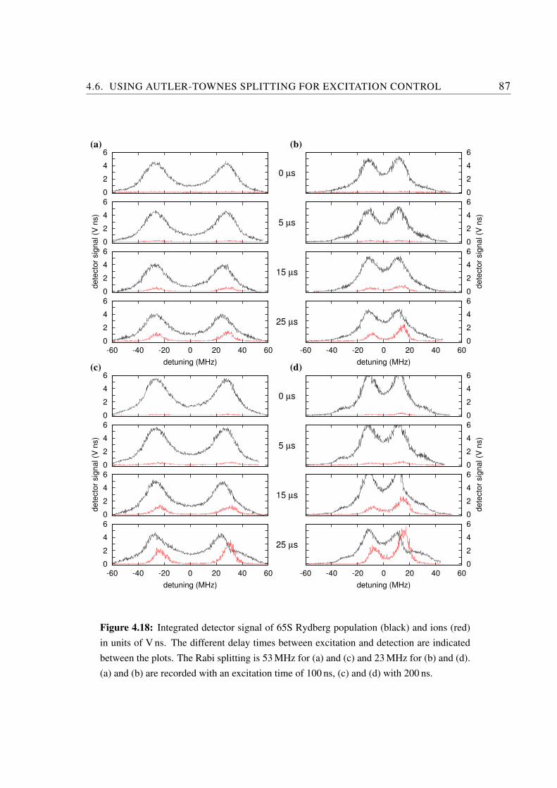
4.6. USING AUTLER-TOWNES SPLITTING FOR EXCITATION CONTROL 87
0
2
4
6
0 µs
(a)
0
2
4
6
5 µs
0
2
4
6
15 µs
0
2
4
6
-60 -40 -20 0 20 40 60
detuning (MHz)
25 µs
dete
cto
r sig
nal (V
ns)
0
2
4
6
0 µs
(c)
0
2
4
6
5 µs
0
2
4
6
15 µs
0
2
4
6
-60 -40 -20 0 20 40 60
detuning (MHz)
25 µs
dete
cto
r sig
nal (V
ns)
0
2
4
6(b)
0
2
4
6
0
2
4
6
-60 -40 -20 0 20 40 600
2
4
6
detuning (MHz)
dete
cto
r sig
nal (V
ns)
0
2
4
6(d)
0
2
4
6
0
2
4
6
-60 -40 -20 0 20 40 600
2
4
6
detuning (MHz)
dete
cto
r sig
nal (V
ns)
Figure 4.18: Integrated detector signal of 65S Rydberg population (black) and ions (red)
in units of V ns. The different delay times between excitation and detection are indicated
between the plots. The Rabi splitting is 53 MHz for (a) and (c) and 23 MHz for (b) and (d).
(a) and (b) are recorded with an excitation time of 100 ns, (c) and (d) with 200 ns.
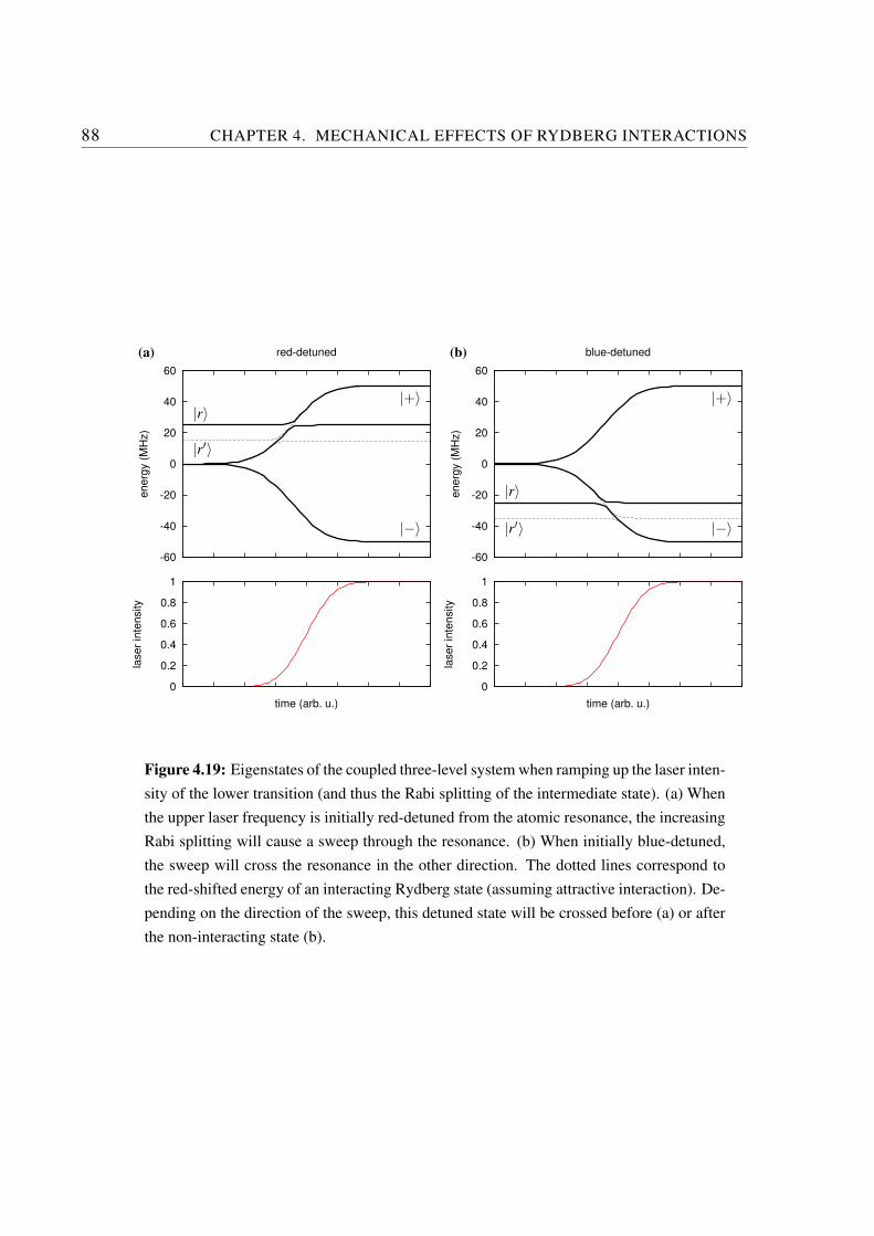
88 CHAPTER 4. MECHANICAL EFFECTS OF RYDBERG INTERACTIONS
-60
-40
-20
0
20
40
60
energ
y (
MH
z)
red-detuned(a)
-60
-40
-20
0
20
40
60
energ
y (
MH
z)
blue-detuned(b)
0
0.2
0.4
0.6
0.8
1
laser
inte
nsity
time (arb. u.)
0
0.2
0.4
0.6
0.8
1
laser
inte
nsity
time (arb. u.)
|r〉
|r〉
|r′〉
|r′〉
|+〉|+〉
|−〉|−〉
Figure 4.19: Eigenstates of the coupled three-level system when ramping up the laser inten-
sity of the lower transition (and thus the Rabi splitting of the intermediate state). (a) When
the upper laser frequency is initially red-detuned from the atomic resonance, the increasing
Rabi splitting will cause a sweep through the resonance. (b) When initially blue-detuned,
the sweep will cross the resonance in the other direction. The dotted lines correspond to
the red-shifted energy of an interacting Rydberg state (assuming attractive interaction). De-
pending on the direction of the sweep, this detuned state will be crossed before (a) or after
the non-interacting state (b).
4.6. USING AUTLER-TOWNES SPLITTING FOR EXCITATION CONTROL 89
0
0.2
0.4
0.6
0.8
1
1.2
1.4
0 0.5 1 1.5 2
photo
dio
de s
ignal (a
rb. u.)
time (µs)
480 nm
780 nm
Figure 4.20: Excitation laser pulse shapes recorded with a fast photodiode. Both pulses
are 500 ns wide and shifted by ∼250 ns relative to each other, so that the increase of the
red laser intensity causes a frequency sweep in the upper transition. The traces are offset
vertically for clarity.
across the Rydberg resonance from lower to higher energies, while the transition from the
other component is far red-detuned (Fig. 4.19(a)). For a blue-detuned excitation laser the
transition from the lower Autler-Townes component crosses the resonance and the chirp
direction is reversed (Fig. 4.19(b)).
The solid lines in Fig. 4.19 correspond to the eigenstates of the system with a detuning
δ2 = ±25MHz of the upper transition. The dashed lines represent a Rydberg state which
experiences an interaction-induced shift by −10MHz, corresponding to an attractive in-
teraction with a nearby Rydberg atom. In case (a) this additional state is crossed before
the non-interacting resonance, so that it cannot be populated (no interaction partners are
present at that time). In case (b) Rydberg atoms are excited on the atomic resonance first,
and the sweep follows the interaction potential to lower frequencies, so that interacting
atoms can subsequently be excited. The expected differences in the pair distribution can
again be probed by recording the ionizing collisions after different delay times.
Fig. 4.21 shows a measurement of the Rydberg excitation and collisional ionization
of the 62D state when scanning the upper laser frequency. The blue excitation pulse is
500 ns wide at a power of ∼35 mW, and the intensity of the red laser is ramped up dur-
ing approximately 80 ns in the center of the blue excitation pulse, as shown in Fig. 4.20.
The maximum Rabi frequency of the red laser is 140 MHz. The Rydberg excitation line
looks somewhat similar to the Autler-Townes spectrum without chirp shown in Fig. 4.16,
because most of the excitation is produced when the red laser intensity is already at its
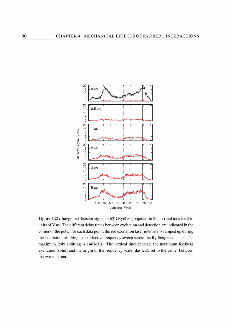
90 CHAPTER 4. MECHANICAL EFFECTS OF RYDBERG INTERACTIONS
0
5
10
15
200 µs
0
5
10
15
200.5 µs
0
5
10
15
201 µs
0
5
10
15
202 µs
0
5
10
15
203 µs
0
5
10
15
20
-100 -75 -50 -25 0 25 50 75 100
detuning (MHz)
5 µs
dete
cto
r sig
nal (V
ns)
Figure 4.21: Integrated detector signal of 62D Rydberg population (black) and ions (red) in
units of V ns. The different delay times between excitation and detection are indicated in the
corner of the pots. For each data point, the red excitation laser intensity is ramped up during
the excitation, resulting in an effective frequency sweep across the Rydberg resonance. The
maximum Rabi splitting is 140 MHz. The vertical lines indicate the maximum Rydberg
excitation (solid) and the origin of the frequency scale (dashed), set to the center between
the two maxima.
4.6. USING AUTLER-TOWNES SPLITTING FOR EXCITATION CONTROL 91
highest value and the blue excitation laser is still turned on. However, some more ex-
citation is visible between the two outer peaks, because the upper transition is always
sweeped across the resonance for a short time. The origin of the frequency scale is cho-
sen to be centered between the two Rydberg maxima, and vertical lines at 0 and ±70 MHz
have been drawn into the plots to guide the eye. The interesting regions in the spectrum
lie in the ranges from 25 MHz to 50 MHz to both sides of the origin, where the only exci-
tation takes place while the transition is quickly sweeped across the resonance. Due to the
attractive van der Waals interaction of the 62D state, the increasing Rydberg population
allows to access more and more atom pairs at shorter distances while the sweep contin-
ues. On the other hand, a sweep in the opposite direction only allows for the excitation of
separated atoms, because the interactions push the energy levels away from the resonance.
It is clearly visible that during the first few microseconds, most ions appear in the re-
gion of positive detuning. Even though the absolute number of Rydberg atoms is highest
at the two outer peaks in the spectrum, the number of collisions is higher in the inter-
mediate region at positive detunings. This suggests that far more close pairs exist in this
region, in accordance with the expectation that a chirp from high to low energy excites
atoms at short distance.
In addition to the transition being sweeped through the Rydberg resonance, the second
component of the Autler-Townes doublet enables far-detuned transitions in the same way
as described in Sec. 4.6.1. This explains the asymmetric behavior in the ionization of the
outer peaks in the spectrum, where the peak at negative detuning ionizes more strongly.
Fast chirps of the excitation laser frequency have been used to control the collision
rate of rubidium ground state atoms in a magneto-optical trap [Wright et al., 2005,Wright
et al., 2007]. The approach presented here is a similar scheme for controlling collisions of
Rydberg atoms by influencing the pair distribution. The results show that fast frequency
chirps can be achieved without the need for varying the laser frequency and that the pair
distribution of the excited state atoms can be influenced by the chirp direction. Motion
on the attractive potentials happens on a timescale of microseconds, while the frequency
sweep itself acts on the system within 50 ns. Interference effects of a moving wave packet
due to multiple interactions with the light field as observed by [Wright et al., 2007] in
a ground-state system will therefore not be of relevance here. Instead, a description in
terms of subsequently excited Rydberg atoms forming a specific pair distribution seems
more appropriate.
In future experiments, the sweep rate could be changed by implementing a fast con-

92 CHAPTER 4. MECHANICAL EFFECTS OF RYDBERG INTERACTIONS
trolled attenuator to vary the AOM power instead of a switch. This should allow one to
investigate the regime where the sweep follows the atomic motion in real time.
Chapter 5
Coherence in Rydberg gases
The results of the previous chapter have shown that the mechanical motion induced by
the long-range interactions in a Rydberg gas can be understood in a picture of classical
accelerated particles and that the dynamics of the system can be controlled to some degree
by appropriate detuning of the excitation.
It remains to be investigated how the system can be prepared in a well-known quantum
state or superposition, and how the coherent evolution of the system can be described and
controlled. At the same time it must be considered in how far coherence is affected by
interaction-induced motion.
Sec. 5.1 and Sec. 5.2 focus on the coherent evolution of atomic states coupled to the
excitation light field. The atom-light interaction is described in terms of the Optical Bloch
Equations. Experimental techniques for the observation of coherent excitation effects are
described and two manifestations of quantum mechanical coherence, Rabi oscillations
and Ramsey interference, are discussed.
The remaining sections explore the coherent character of Rydberg interactions in
many-particle systems. In Sec. 5.3 the dynamics of resonant energy transfer in an un-
ordered gas is examined with a few-body Monte Carlo model which is compared to exper-
imental results. In Sec. 5.4 and Sec. 5.5 the coherent energy transfer in one-dimensional
chains is discussed and an experimental realization of such a system is proposed. The
influence of interaction-induced motion on the evolution of these systems is also consid-
ered.
93
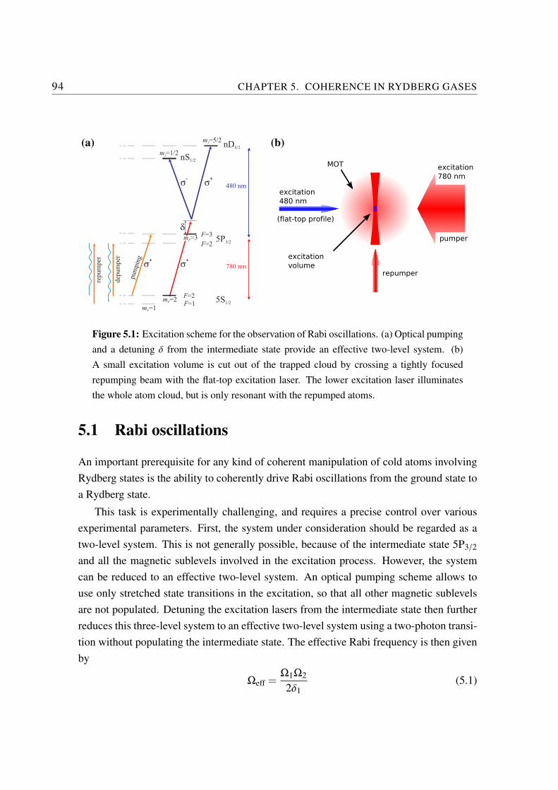
94 CHAPTER 5. COHERENCE IN RYDBERG GASES
5P3/2
d
5S1/2
F=2
F=1
F=3
mF=1
mF=2
F=2
nD5/2
nS1/2
mF=3
mJ=1/2
mJ=5/2
s+
s+
s+
s-
dep
um
per
repum
per
480 nm
780 nm
pum
pin
g(a)
excitation
480 nm
repumper
excitation
780 nm
pumper
excitation
volume
MOT
(flat−top profile)
(b)
Figure 5.1: Excitation scheme for the observation of Rabi oscillations. (a) Optical pumping
and a detuning δ from the intermediate state provide an effective two-level system. (b)
A small excitation volume is cut out of the trapped cloud by crossing a tightly focused
repumping beam with the flat-top excitation laser. The lower excitation laser illuminates
the whole atom cloud, but is only resonant with the repumped atoms.
5.1 Rabi oscillations
An important prerequisite for any kind of coherent manipulation of cold atoms involving
Rydberg states is the ability to coherently drive Rabi oscillations from the ground state to
a Rydberg state.
This task is experimentally challenging, and requires a precise control over various
experimental parameters. First, the system under consideration should be regarded as a
two-level system. This is not generally possible, because of the intermediate state 5P3/2
and all the magnetic sublevels involved in the excitation process. However, the system
can be reduced to an effective two-level system. An optical pumping scheme allows to
use only stretched state transitions in the excitation, so that all other magnetic sublevels
are not populated. Detuning the excitation lasers from the intermediate state then further
reduces this three-level system to an effective two-level system using a two-photon transi-
tion without populating the intermediate state. The effective Rabi frequency is then given
by
Ωeff =Ω1Ω2
2δ1(5.1)
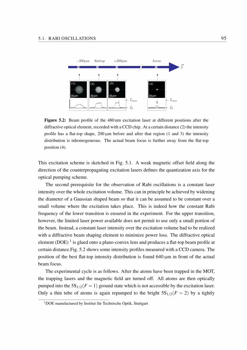
5.1. RABI OSCILLATIONS 95
50 mm 50 mm 50 mm 50 mm
(1) (2) (3) (4)
~z
Imax Imax
I0 I0
−200µm flattop +200µm focus
Figure 5.2: Beam profile of the 480 nm excitation laser at different positions after the
diffractive optical element, recorded with a CCD chip. At a certain distance (2) the intensity
profile has a flat-top shape, 200 µm before and after that region (1 and 3) the intensity
distribution is inhomogeneous. The actual beam focus is further away from the flat-top
position (4).
This excitation scheme is sketched in Fig. 5.1. A weak magnetic offset field along the
direction of the counterpropagating excitation lasers defines the quantization axis for the
optical pumping scheme.
The second prerequisite for the observation of Rabi oscillations is a constant laser
intensity over the whole excitation volume. This can in principle be achieved by widening
the diameter of a Gaussian shaped beam so that it can be assumed to be constant over a
small volume where the excitation takes place. This is indeed how the constant Rabi
frequency of the lower transition is ensured in the experiment. For the upper transition,
however, the limited laser power available does not permit to use only a small portion of
the beam. Instead, a constant laser intensity over the excitation volume had to be realized
with a diffractive beam shaping element to minimize power loss. The diffractive optical
element (DOE) 1 is glued onto a plano-convex lens and produces a flat-top beam profile at
certain distance.Fig. 5.2 shows some intensity profiles measured with a CCD camera. The
position of the best flat-top intensity distribution is found 640 µm in front of the actual
beam focus.
The experimental cycle is as follows. After the atoms have been trapped in the MOT,
the trapping lasers and the magnetic field are turned off. All atoms are then optically
pumped into the 5S1/2(F = 1) ground state which is not accessible by the excitation laser.
Only a thin tube of atoms is again repumped to the bright 5S1/2(F = 2) by a tightly
1DOE manufactured by Institut fur Technische Optik, Stuttgart
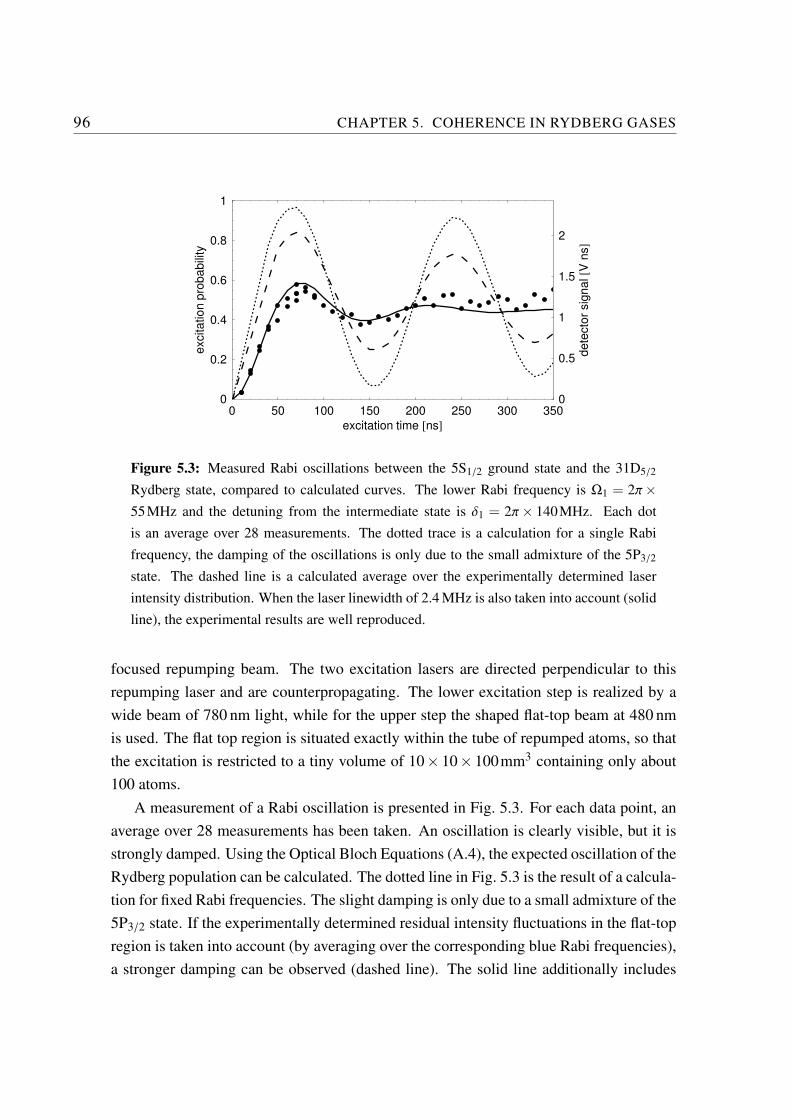
96 CHAPTER 5. COHERENCE IN RYDBERG GASES
0 50 100 150 200 250 300 350
excitation time @nsD
0
0.2
0.4
0.6
0.8
1e
xcita
tio
np
rob
ab
ility
0
0.5
1
1.5
2
de
tecto
rsig
na
l@V
nsD
Figure 5.3: Measured Rabi oscillations between the 5S1/2 ground state and the 31D5/2
Rydberg state, compared to calculated curves. The lower Rabi frequency is Ω1 = 2π×55MHz and the detuning from the intermediate state is δ1 = 2π× 140MHz. Each dot
is an average over 28 measurements. The dotted trace is a calculation for a single Rabi
frequency, the damping of the oscillations is only due to the small admixture of the 5P3/2
state. The dashed line is a calculated average over the experimentally determined laser
intensity distribution. When the laser linewidth of 2.4 MHz is also taken into account (solid
line), the experimental results are well reproduced.
focused repumping beam. The two excitation lasers are directed perpendicular to this
repumping laser and are counterpropagating. The lower excitation step is realized by a
wide beam of 780 nm light, while for the upper step the shaped flat-top beam at 480 nm
is used. The flat top region is situated exactly within the tube of repumped atoms, so that
the excitation is restricted to a tiny volume of 10× 10× 100mm3 containing only about
100 atoms.
A measurement of a Rabi oscillation is presented in Fig. 5.3. For each data point, an
average over 28 measurements has been taken. An oscillation is clearly visible, but it is
strongly damped. Using the Optical Bloch Equations (A.4), the expected oscillation of the
Rydberg population can be calculated. The dotted line in Fig. 5.3 is the result of a calcula-
tion for fixed Rabi frequencies. The slight damping is only due to a small admixture of the
5P3/2 state. If the experimentally determined residual intensity fluctuations in the flat-top
region is taken into account (by averaging over the corresponding blue Rabi frequencies),
a stronger damping can be observed (dashed line). The solid line additionally includes
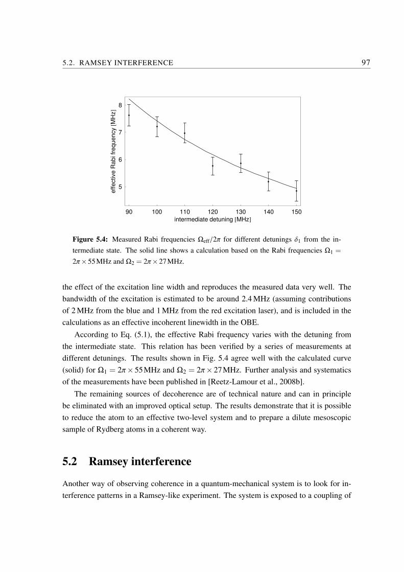
5.2. RAMSEY INTERFERENCE 97
90 100 110 120 130 140 150
intermediate detuning @MHzD
5
6
7
8
eff
ective
Ra
bifr
eq
ue
ncy@M
HzD
Figure 5.4: Measured Rabi frequencies Ωeff/2π for different detunings δ1 from the in-
termediate state. The solid line shows a calculation based on the Rabi frequencies Ω1 =
2π×55MHz and Ω2 = 2π×27MHz.
the effect of the excitation line width and reproduces the measured data very well. The
bandwidth of the excitation is estimated to be around 2.4 MHz (assuming contributions
of 2 MHz from the blue and 1 MHz from the red excitation laser), and is included in the
calculations as an effective incoherent linewidth in the OBE.
According to Eq. (5.1), the effective Rabi frequency varies with the detuning from
the intermediate state. This relation has been verified by a series of measurements at
different detunings. The results shown in Fig. 5.4 agree well with the calculated curve
(solid) for Ω1 = 2π× 55MHz and Ω2 = 2π× 27MHz. Further analysis and systematics
of the measurements have been published in [Reetz-Lamour et al., 2008b].
The remaining sources of decoherence are of technical nature and can in principle
be eliminated with an improved optical setup. The results demonstrate that it is possible
to reduce the atom to an effective two-level system and to prepare a dilute mesoscopic
sample of Rydberg atoms in a coherent way.
5.2 Ramsey interference
Another way of observing coherence in a quantum-mechanical system is to look for in-
terference patterns in a Ramsey-like experiment. The system is exposed to a coupling of
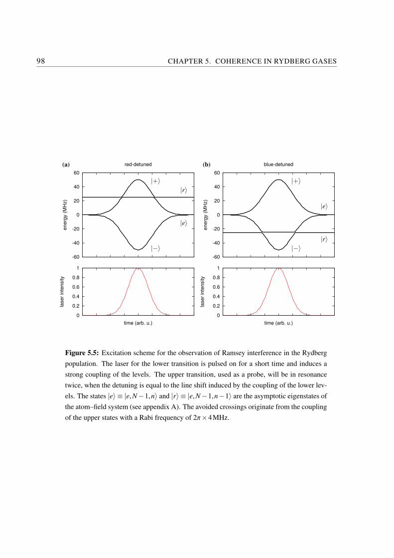
98 CHAPTER 5. COHERENCE IN RYDBERG GASES
-60
-40
-20
0
20
40
60
energ
y (
MH
z)
red-detuned(a)
-60
-40
-20
0
20
40
60
energ
y (
MH
z)
blue-detuned(b)
0
0.2
0.4
0.6
0.8
1
laser
inte
nsity
time (arb. u.)
0
0.2
0.4
0.6
0.8
1
laser
inte
nsity
time (arb. u.)
|r〉
|r〉
|e〉
|e〉
|+〉|+〉
|−〉|−〉
Figure 5.5: Excitation scheme for the observation of Ramsey interference in the Rydberg
population. The laser for the lower transition is pulsed on for a short time and induces a
strong coupling of the levels. The upper transition, used as a probe, will be in resonance
twice, when the detuning is equal to the line shift induced by the coupling of the lower lev-
els. The states |e〉 ≡ |e,N−1,n〉 and |r〉 ≡ |e,N−1,n−1〉 are the asymptotic eigenstates of
the atom–field system (see appendix A). The avoided crossings originate from the coupling
of the upper states with a Rabi frequency of 2π×4MHz.
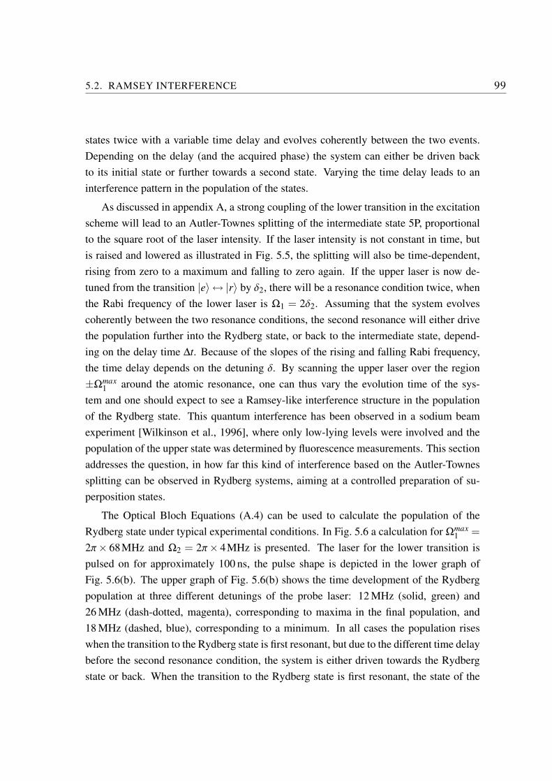
5.2. RAMSEY INTERFERENCE 99
states twice with a variable time delay and evolves coherently between the two events.
Depending on the delay (and the acquired phase) the system can either be driven back
to its initial state or further towards a second state. Varying the time delay leads to an
interference pattern in the population of the states.
As discussed in appendix A, a strong coupling of the lower transition in the excitation
scheme will lead to an Autler-Townes splitting of the intermediate state 5P, proportional
to the square root of the laser intensity. If the laser intensity is not constant in time, but
is raised and lowered as illustrated in Fig. 5.5, the splitting will also be time-dependent,
rising from zero to a maximum and falling to zero again. If the upper laser is now de-
tuned from the transition |e〉 ↔ |r〉 by δ2, there will be a resonance condition twice, when
the Rabi frequency of the lower laser is Ω1 = 2δ2. Assuming that the system evolves
coherently between the two resonance conditions, the second resonance will either drive
the population further into the Rydberg state, or back to the intermediate state, depend-
ing on the delay time ∆t. Because of the slopes of the rising and falling Rabi frequency,
the time delay depends on the detuning δ. By scanning the upper laser over the region
±Ωmax1 around the atomic resonance, one can thus vary the evolution time of the sys-
tem and one should expect to see a Ramsey-like interference structure in the population
of the Rydberg state. This quantum interference has been observed in a sodium beam
experiment [Wilkinson et al., 1996], where only low-lying levels were involved and the
population of the upper state was determined by fluorescence measurements. This section
addresses the question, in how far this kind of interference based on the Autler-Townes
splitting can be observed in Rydberg systems, aiming at a controlled preparation of su-
perposition states.
The Optical Bloch Equations (A.4) can be used to calculate the population of the
Rydberg state under typical experimental conditions. In Fig. 5.6 a calculation for Ωmax1 =
2π× 68MHz and Ω2 = 2π× 4MHz is presented. The laser for the lower transition is
pulsed on for approximately 100 ns, the pulse shape is depicted in the lower graph of
Fig. 5.6(b). The upper graph of Fig. 5.6(b) shows the time development of the Rydberg
population at three different detunings of the probe laser: 12 MHz (solid, green) and
26 MHz (dash-dotted, magenta), corresponding to maxima in the final population, and
18 MHz (dashed, blue), corresponding to a minimum. In all cases the population rises
when the transition to the Rydberg state is first resonant, but due to the different time delay
before the second resonance condition, the system is either driven towards the Rydberg
state or back. When the transition to the Rydberg state is first resonant, the state of the
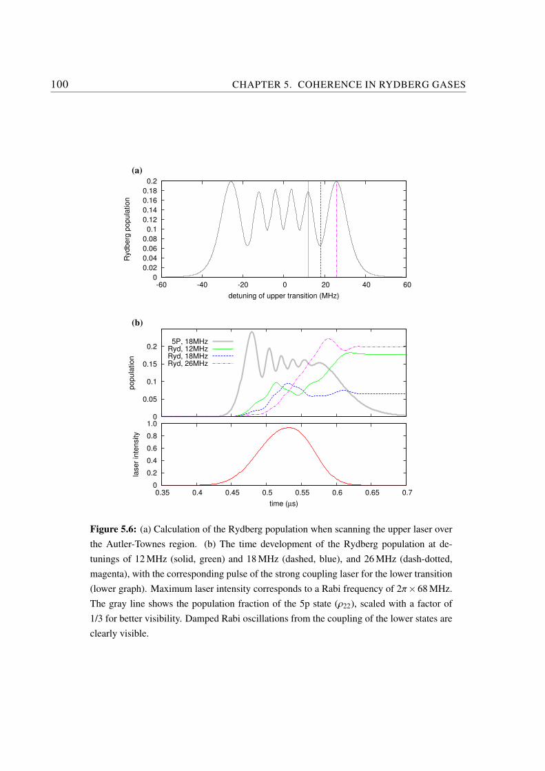
100 CHAPTER 5. COHERENCE IN RYDBERG GASES
0
0.02
0.04
0.06
0.08
0.1
0.12
0.14
0.16
0.18
0.2
-60 -40 -20 0 20 40 60
Rydberg
popula
tion
detuning of upper transition (MHz)
(a)
0
0.05
0.1
0.15
0.2
popula
tion
(b)
5P, 18MHzRyd, 12MHzRyd, 18MHzRyd, 26MHz
0
0.2
0.4
0.6
0.8
1.0
0.35 0.4 0.45 0.5 0.55 0.6 0.65 0.7
laser
inte
nsity
time (µs)
Figure 5.6: (a) Calculation of the Rydberg population when scanning the upper laser over
the Autler-Townes region. (b) The time development of the Rydberg population at de-
tunings of 12 MHz (solid, green) and 18 MHz (dashed, blue), and 26 MHz (dash-dotted,
magenta), with the corresponding pulse of the strong coupling laser for the lower transition
(lower graph). Maximum laser intensity corresponds to a Rabi frequency of 2π×68 MHz.
The gray line shows the population fraction of the 5p state (ρ22), scaled with a factor of
1/3 for better visibility. Damped Rabi oscillations from the coupling of the lower states are
clearly visible.
5.2. RAMSEY INTERFERENCE 101
0
5
10
15
20
25
-200 -150 -100 -50 0 50 100 150 200
photo
dio
de s
ignal (a
rb.u
.)
time (ns)
Figure 5.7: Measured pulse shapes of the two excitation lasers. The laser for the lower
transition (780 nm, red trace) is switched with an AOM, the laser for the upper transition
(480 nm, blue trace) is switched with a Pockels cell. The pulse shapes can be well repro-
duced with error functions fitted to the slopes. The pulse length of the red laser is 80 ns in
this example (delay between the switching TTL pulses).
system splits in two branches (see Fig. 5.6), which interfere again at the second resonance.
One of the branches is the Rydberg state itself, the other one does not contain much
admixture of the Rydberg state, and is mainly a superposition of the two lower states |g〉and |e〉. The population of |e〉 (given by the density matrix element ρ22 in the notation
of appendix A) is shown as the gray line in Fig. 5.6(b) (scaled by 1/3). It reflects the
Rabi oscillation between the strongly coupled states |g〉 and |e〉, and its phase at the time
of the second resonance condition determines the further development of the Rydberg
population. The oscillations of |g〉 are strongly damped due to the finite lifetime of the
5P state. This damping is responsible for the limited visibility of the Ramsey fringes in
Fig. 5.6(a).
The laser pulse shape shown in Fig. 5.6 is derived from a measurement of the pulse
shape realized in the experiment by fitting two error functions to the slopes. The measured
pulse shapes of both excitation lasers (upper and lower transition) are shown in Fig. 5.7.
While the laser for the lower transition (780 nm) is switched with an AOM, a Pockels cell
is used to switch the upper transition laser (480 nm), resulting in much steeper slopes.
Both pulses are measured successively with the same high-bandwidth photodiode to en-
sure that the relative time delay between the pulses is monitored correctly. The pulse
width of the excitation lasers can be varied to investigate a larger range of time delays
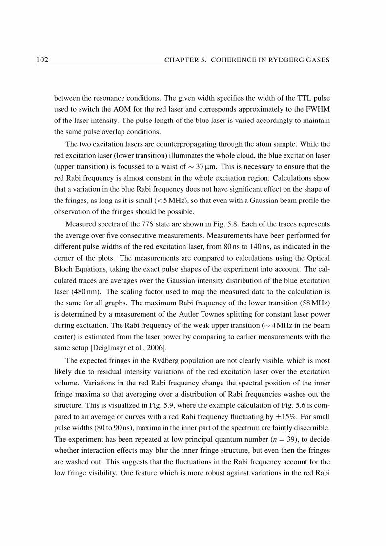
102 CHAPTER 5. COHERENCE IN RYDBERG GASES
between the resonance conditions. The given width specifies the width of the TTL pulse
used to switch the AOM for the red laser and corresponds approximately to the FWHM
of the laser intensity. The pulse length of the blue laser is varied accordingly to maintain
the same pulse overlap conditions.
The two excitation lasers are counterpropagating through the atom sample. While the
red excitation laser (lower transition) illuminates the whole cloud, the blue excitation laser
(upper transition) is focussed to a waist of ∼ 37µm. This is necessary to ensure that the
red Rabi frequency is almost constant in the whole excitation region. Calculations show
that a variation in the blue Rabi frequency does not have significant effect on the shape of
the fringes, as long as it is small (< 5 MHz), so that even with a Gaussian beam profile the
observation of the fringes should be possible.
Measured spectra of the 77S state are shown in Fig. 5.8. Each of the traces represents
the average over five consecutive measurements. Measurements have been performed for
different pulse widths of the red excitation laser, from 80 ns to 140 ns, as indicated in the
corner of the plots. The measurements are compared to calculations using the Optical
Bloch Equations, taking the exact pulse shapes of the experiment into account. The cal-
culated traces are averages over the Gaussian intensity distribution of the blue excitation
laser (480 nm). The scaling factor used to map the measured data to the calculation is
the same for all graphs. The maximum Rabi frequency of the lower transition (58 MHz)
is determined by a measurement of the Autler Townes splitting for constant laser power
during excitation. The Rabi frequency of the weak upper transition (∼ 4MHz in the beam
center) is estimated from the laser power by comparing to earlier measurements with the
same setup [Deiglmayr et al., 2006].
The expected fringes in the Rydberg population are not clearly visible, which is most
likely due to residual intensity variations of the red excitation laser over the excitation
volume. Variations in the red Rabi frequency change the spectral position of the inner
fringe maxima so that averaging over a distribution of Rabi frequencies washes out the
structure. This is visualized in Fig. 5.9, where the example calculation of Fig. 5.6 is com-
pared to an average of curves with a red Rabi frequency fluctuating by ±15%. For small
pulse widths (80 to 90 ns), maxima in the inner part of the spectrum are faintly discernible.
The experiment has been repeated at low principal quantum number (n = 39), to decide
whether interaction effects may blur the inner fringe structure, but even then the fringes
are washed out. This suggests that the fluctuations in the Rabi frequency account for the
low fringe visibility. One feature which is more robust against variations in the red Rabi
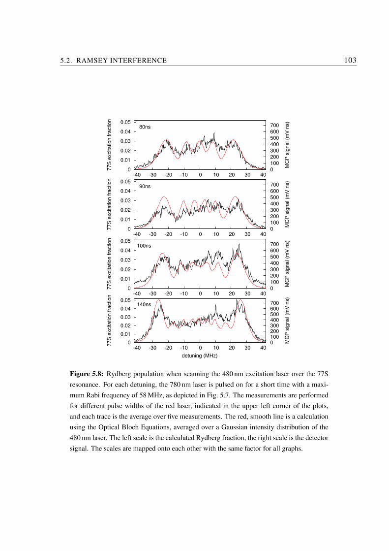
5.2. RAMSEY INTERFERENCE 103
0
0.01
0.02
0.03
0.04
0.05
-40 -30 -20 -10 0 10 20 30 40 0
100
200
300
400
500
600
700
77S
excitation fra
ction
MC
P s
ignal (m
V n
s)
80ns
0
0.01
0.02
0.03
0.04
0.05
-40 -30 -20 -10 0 10 20 30 40 0
100
200
300
400
500
600
700
77S
excitation fra
ction
MC
P s
ignal (m
V n
s)
90ns
0
0.01
0.02
0.03
0.04
0.05
-40 -30 -20 -10 0 10 20 30 40 0
100
200
300
400
500
600
700
77S
excitation fra
ction
MC
P s
ignal (m
V n
s)
100ns
0
0.01
0.02
0.03
0.04
0.05
-40 -30 -20 -10 0 10 20 30 40 0 100 200 300 400 500 600 700
77S
excitation fra
ction
MC
P s
ignal (m
V n
s)
detuning (MHz)
140ns
Figure 5.8: Rydberg population when scanning the 480 nm excitation laser over the 77S
resonance. For each detuning, the 780 nm laser is pulsed on for a short time with a maxi-
mum Rabi frequency of 58 MHz, as depicted in Fig. 5.7. The measurements are performed
for different pulse widths of the red laser, indicated in the upper left corner of the plots,
and each trace is the average over five measurements. The red, smooth line is a calculation
using the Optical Bloch Equations, averaged over a Gaussian intensity distribution of the
480 nm laser. The left scale is the calculated Rydberg fraction, the right scale is the detector
signal. The scales are mapped onto each other with the same factor for all graphs.
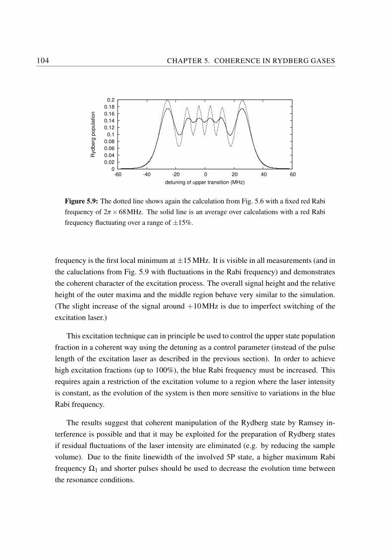
104 CHAPTER 5. COHERENCE IN RYDBERG GASES
0
0.02
0.04
0.06
0.08
0.1
0.12
0.14
0.16
0.18
0.2
-60 -40 -20 0 20 40 60
Rydberg
popula
tion
detuning of upper transition (MHz)
Figure 5.9: The dotted line shows again the calculation from Fig. 5.6 with a fixed red Rabi
frequency of 2π× 68MHz. The solid line is an average over calculations with a red Rabi
frequency fluctuating over a range of ±15%.
frequency is the first local minimum at ±15 MHz. It is visible in all measurements (and in
the caluclations from Fig. 5.9 with fluctuations in the Rabi frequency) and demonstrates
the coherent character of the excitation process. The overall signal height and the relative
height of the outer maxima and the middle region behave very similar to the simulation.
(The slight increase of the signal around +10MHz is due to imperfect switching of the
excitation laser.)
This excitation technique can in principle be used to control the upper state population
fraction in a coherent way using the detuning as a control parameter (instead of the pulse
length of the excitation laser as described in the previous section). In order to achieve
high excitation fractions (up to 100%), the blue Rabi frequency must be increased. This
requires again a restriction of the excitation volume to a region where the laser intensity
is constant, as the evolution of the system is then more sensitive to variations in the blue
Rabi frequency.
The results suggest that coherent manipulation of the Rydberg state by Ramsey in-
terference is possible and that it may be exploited for the preparation of Rydberg states
if residual fluctuations of the laser intensity are eliminated (e.g. by reducing the sample
volume). Due to the finite linewidth of the involved 5P state, a higher maximum Rabi
frequency Ω1 and shorter pulses should be used to decrease the evolution time between
the resonance conditions.
5.3. RESONANT ENERGY TRANSFER IN AN UNORDERED GAS 105
5.3 Resonant energy transfer in an unordered gas
Apart from the coherent interaction of the atom with the light fields described in the pre-
vious sections, coherence can also be observed in the dipole interaction between Rydberg
atoms. This section focuses on the coherent transfer of population among Rydberg atoms
by resonant dipole coupling. This process has been introduced in Sec. 3.1.1 for atom pairs,
where it has been found that the electric field can be used to switch on a resonance condi-
tion between two different pair states. Here the description is extended to many-particle
systems.
In an unordered gas of Rydberg atoms, the distribution of distances between the atoms
accounts for a large variation of interaction strengths. Coherent population oscillations of
the involved states are therefore washed out and can not be directly observed experimen-
tally. Still the total fraction of population in one or the other state can be measured and
the time evolution of the many-body system can be investigated.
5.3.1 Many-body model of resonant energy transfer
To model the dynamics of an unordered gas, consider a sub-ensemble of N atoms at
random positions. Each atom has three different internal states, p, s, and s′, so that the
total number of many-particle states is 3N . All atoms are prepared in the state p. The
initial many-body state can thus be expressed as
|0〉 = |ppp . . . p〉 . (5.2)
Switching the system to the resonance condition introduces a number of interactions
among the particles. The new Hamiltonian must now be diagonalized to obtain a set
of new eigenfunctions as linear combinations of the unperturbed states. Any two atoms
can change their state from pp to ss′ and vice versa, so that the number of s and s′ atoms
must always be equal. This reduces the number of possible states to be considered in the
model significantly:
number of atoms N 2 3 4 6 8 10
number of states 3 7 19 141 1107 8953
Specifically, the following interactions are considered:
p + p s + s′ (5.3)
106 CHAPTER 5. COHERENCE IN RYDBERG GASES
is the energy transfer process made resonant by tuning the electric field to a Forster res-
onance. This process increases or decreases the number of s atoms. In addition, the
excitation exchange processes
p + s s + p (5.4)
p + s′ s′ + p (5.5)
are included. These processes represent a diffusion of excitation through the cloud. They
are always resonant and conserve the number of s atoms in the sample.
The dipole-dipole interaction is anisotropic and depends on the angle between the
quantization axis (defined by the electric field) and the distance vector ~R between the
atoms. The interaction energies are thus given by
〈pp|V|ss′〉 =~µ~µ′
|~R|3−3
(~µ~R)(~µ′~R)
|~R|5(5.6)
for the energy transfer process (5.3) and
〈ps|V|sp〉 =~µ2
|~R|3−3
(~µ~R)2
|~R|5(5.7)
〈ps′|V|s′p〉 =~µ′2
|~R|3−3
(~µ′~R)2
|~R|5(5.8)
for the energy exchange processes (5.4) and (5.5).
The calculations were adapted to the experimental conditions with the Rydberg states
p = 32P3/2, s = 32S1/2 and s′ = 33S1/2, using the calculated radial dipole matrix ele-
ments µrad = 966au and µ′rad = 943au (see Sec. 2.2). It is further assumed that half of
the atoms are initially in the state 32P3/2(mJ = +3/2) and the other half in the state
32P3/2(mJ =−3/2). Including the Clebsch-Gordan coefficients the only non-zero matrix
for the transition 32P3/2(|mJ| = 3/2)↔32S1/2 in a spherical basis are
µ=∣
∣
∣
⟨
32P 32 ,mJ=+ 3
2
∣
∣
∣µ+
∣
∣
∣32S 12 ,mJ=+ 1
2
⟩∣
∣
∣ (5.9)
=∣
∣
∣
⟨
32P 32 ,mJ=+ 3
2
∣
∣
∣µ+
∣
∣
∣32S 12 ,mJ=+ 1
2
⟩∣
∣
∣
=1√3
µrad
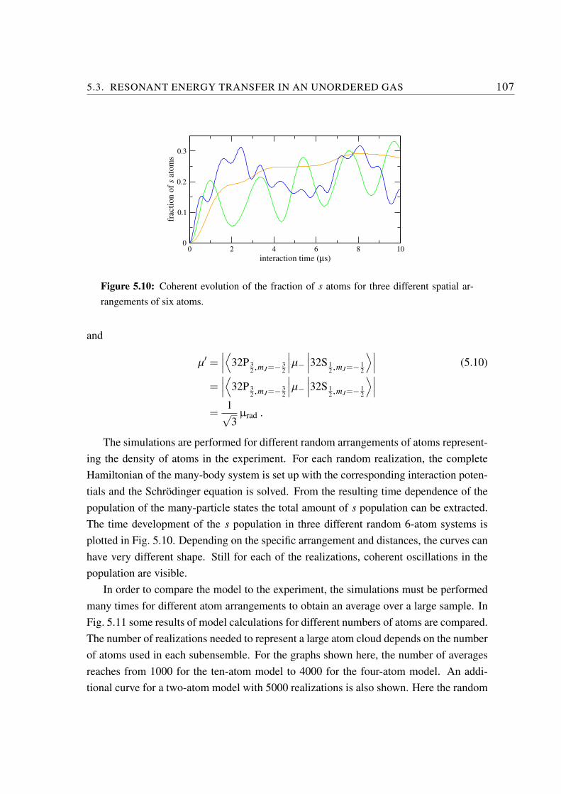
5.3. RESONANT ENERGY TRANSFER IN AN UNORDERED GAS 107
0 2 4 6 8 10
interaction time (µs)
0
0.1
0.2
0.3
frac
tion o
f s
atom
s
Figure 5.10: Coherent evolution of the fraction of s atoms for three different spatial ar-
rangements of six atoms.
and
µ′ =∣
∣
∣
⟨
32P 32 ,mJ=− 3
2
∣
∣
∣µ−∣
∣
∣32S 12 ,mJ=− 1
2
⟩∣
∣
∣ (5.10)
=∣
∣
∣
⟨
32P 32 ,mJ=− 3
2
∣
∣
∣µ−∣
∣
∣32S 12 ,mJ=− 1
2
⟩∣
∣
∣
=1√3
µrad .
The simulations are performed for different random arrangements of atoms represent-
ing the density of atoms in the experiment. For each random realization, the complete
Hamiltonian of the many-body system is set up with the corresponding interaction poten-
tials and the Schrodinger equation is solved. From the resulting time dependence of the
population of the many-particle states the total amount of s population can be extracted.
The time development of the s population in three different random 6-atom systems is
plotted in Fig. 5.10. Depending on the specific arrangement and distances, the curves can
have very different shape. Still for each of the realizations, coherent oscillations in the
population are visible.
In order to compare the model to the experiment, the simulations must be performed
many times for different atom arrangements to obtain an average over a large sample. In
Fig. 5.11 some results of model calculations for different numbers of atoms are compared.
The number of realizations needed to represent a large atom cloud depends on the number
of atoms used in each subensemble. For the graphs shown here, the number of averages
reaches from 1000 for the ten-atom model to 4000 for the four-atom model. An addi-
tional curve for a two-atom model with 5000 realizations is also shown. Here the random
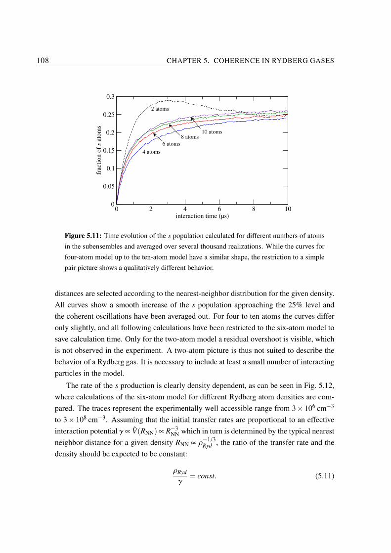
108 CHAPTER 5. COHERENCE IN RYDBERG GASES
0 2 4 6 8 10interaction time (µs)
0
0.05
0.1
0.15
0.2
0.25
0.3fr
acti
on o
f s
atom
s
6 atoms
4 atoms
8 atoms10 atoms
2 atoms
Figure 5.11: Time evolution of the s population calculated for different numbers of atoms
in the subensembles and averaged over several thousand realizations. While the curves for
four-atom model up to the ten-atom model have a similar shape, the restriction to a simple
pair picture shows a qualitatively different behavior.
distances are selected according to the nearest-neighbor distribution for the given density.
All curves show a smooth increase of the s population approaching the 25% level and
the coherent oscillations have been averaged out. For four to ten atoms the curves differ
only slightly, and all following calculations have been restricted to the six-atom model to
save calculation time. Only for the two-atom model a residual overshoot is visible, which
is not observed in the experiment. A two-atom picture is thus not suited to describe the
behavior of a Rydberg gas. It is necessary to include at least a small number of interacting
particles in the model.
The rate of the s production is clearly density dependent, as can be seen in Fig. 5.12,
where calculations of the six-atom model for different Rydberg atom densities are com-
pared. The traces represent the experimentally well accessible range from 3× 106 cm−3
to 3× 108 cm−3. Assuming that the initial transfer rates are proportional to an effective
interaction potential γ∝ V(RNN) ∝ R−3NN which in turn is determined by the typical nearest
neighbor distance for a given density RNN ∝ ρ−1/3Ryd , the ratio of the transfer rate and the
density should be expected to be constant:
ρRyd
γ= const. (5.11)
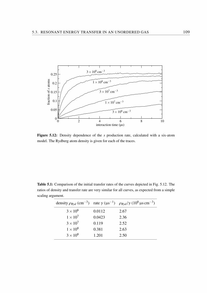
5.3. RESONANT ENERGY TRANSFER IN AN UNORDERED GAS 109
0 2 4 6 8 10interaction time (µs)
0
0.05
0.1
0.15
0.2
0.25
frac
tion o
f s
atom
s
3×108 cm−3
1×108 cm−3
3×107 cm−3
1×107 cm−3
3×106 cm−3
Figure 5.12: Density dependence of the s production rate, calculated with a six-atom
model. The Rydberg atom density is given for each of the traces.
Table 5.1: Comparison of the initial transfer rates of the curves depicted in Fig. 5.12. The
ratios of density and transfer rate are very similar for all curves, as expected from a simple
scaling argument.
density ρRyd (cm−3) rate γ (µs−1) ρRyd/γ (108µs cm−3)
3×10⁶ 0.0112 2.67
1×10⁷ 0.0423 2.36
3×10⁷ 0.119 2.52
1×10⁸ 0.381 2.63
3×10⁸ 1.201 2.50
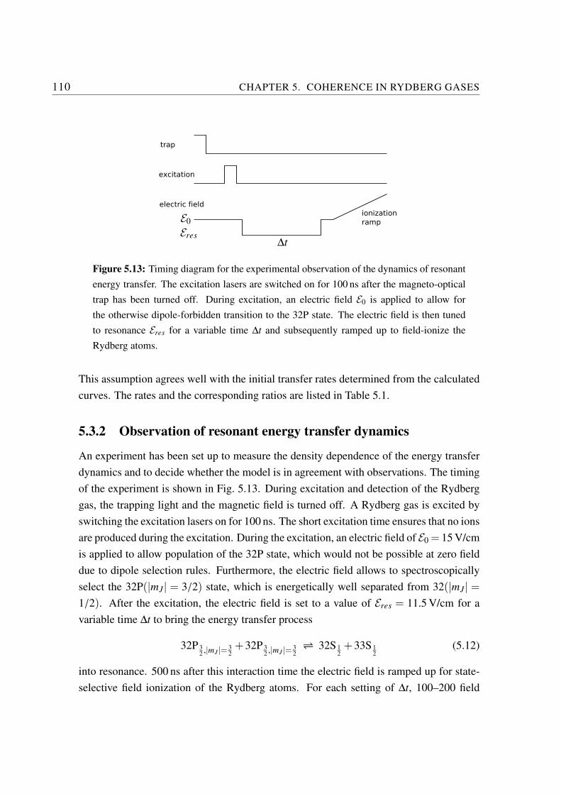
110 CHAPTER 5. COHERENCE IN RYDBERG GASES
excitation
electric field
trap
ionization
ramp
∆t
E0
Eres
Figure 5.13: Timing diagram for the experimental observation of the dynamics of resonant
energy transfer. The excitation lasers are switched on for 100 ns after the magneto-optical
trap has been turned off. During excitation, an electric field E0 is applied to allow for
the otherwise dipole-forbidden transition to the 32P state. The electric field is then tuned
to resonance Eres for a variable time ∆t and subsequently ramped up to field-ionize the
Rydberg atoms.
This assumption agrees well with the initial transfer rates determined from the calculated
curves. The rates and the corresponding ratios are listed in Table 5.1.
5.3.2 Observation of resonant energy transfer dynamics
An experiment has been set up to measure the density dependence of the energy transfer
dynamics and to decide whether the model is in agreement with observations. The timing
of the experiment is shown in Fig. 5.13. During excitation and detection of the Rydberg
gas, the trapping light and the magnetic field is turned off. A Rydberg gas is excited by
switching the excitation lasers on for 100 ns. The short excitation time ensures that no ions
are produced during the excitation. During the excitation, an electric field of E0 = 15 V/cm
is applied to allow population of the 32P state, which would not be possible at zero field
due to dipole selection rules. Furthermore, the electric field allows to spectroscopically
select the 32P(|mJ| = 3/2) state, which is energetically well separated from 32(|mJ| =
1/2). After the excitation, the electric field is set to a value of Eres = 11.5 V/cm for a
variable time ∆t to bring the energy transfer process
32P 32 ,|mJ |= 3
2+32P 3
2 ,|mJ |= 32
32S 12+33S 1
2(5.12)
into resonance. 500 ns after this interaction time the electric field is ramped up for state-
selective field ionization of the Rydberg atoms. For each setting of ∆t, 100–200 field
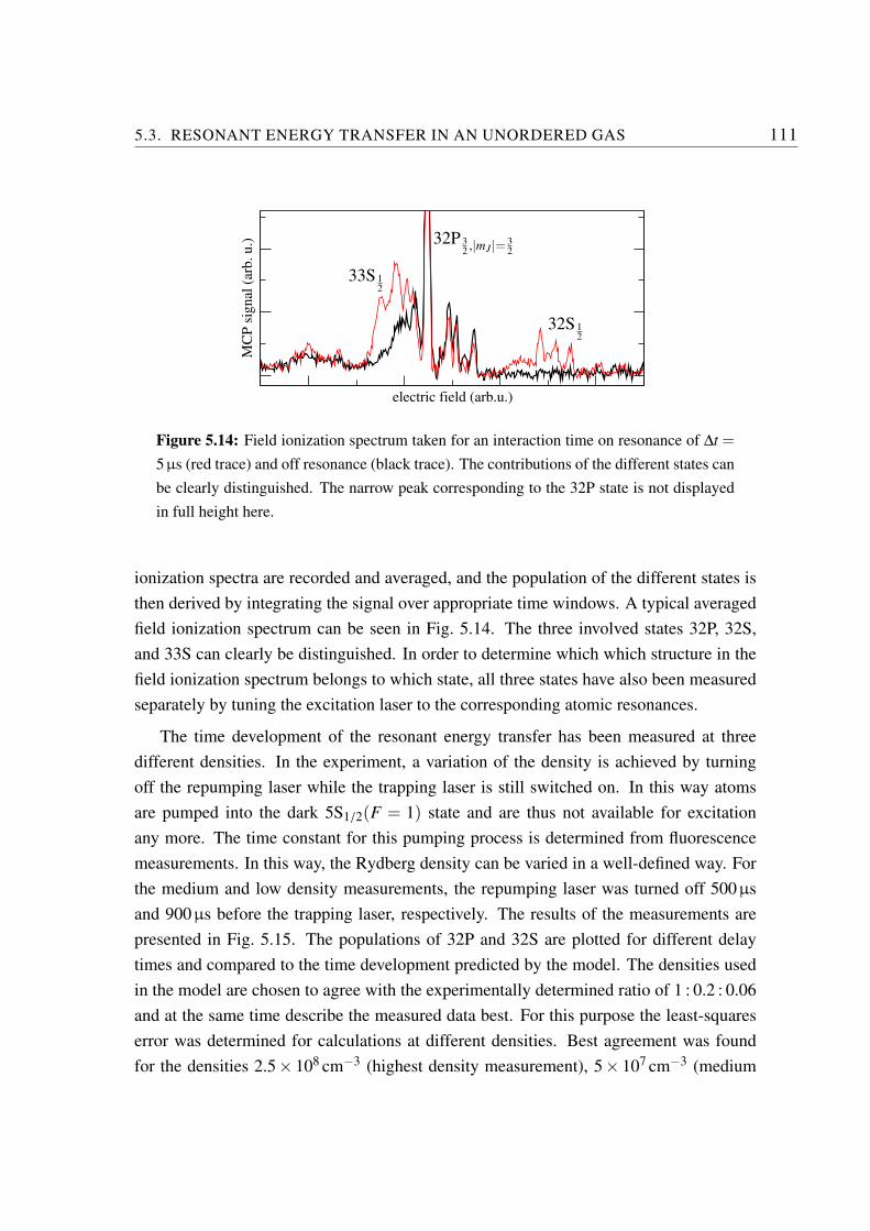
5.3. RESONANT ENERGY TRANSFER IN AN UNORDERED GAS 111
electric field (arb.u.)
MC
P s
ignal
(ar
b. u.) 32P 3
2 ,|mJ |= 32
32S 12
33S 12
Figure 5.14: Field ionization spectrum taken for an interaction time on resonance of ∆t =
5µs (red trace) and off resonance (black trace). The contributions of the different states can
be clearly distinguished. The narrow peak corresponding to the 32P state is not displayed
in full height here.
ionization spectra are recorded and averaged, and the population of the different states is
then derived by integrating the signal over appropriate time windows. A typical averaged
field ionization spectrum can be seen in Fig. 5.14. The three involved states 32P, 32S,
and 33S can clearly be distinguished. In order to determine which which structure in the
field ionization spectrum belongs to which state, all three states have also been measured
separately by tuning the excitation laser to the corresponding atomic resonances.
The time development of the resonant energy transfer has been measured at three
different densities. In the experiment, a variation of the density is achieved by turning
off the repumping laser while the trapping laser is still switched on. In this way atoms
are pumped into the dark 5S1/2(F = 1) state and are thus not available for excitation
any more. The time constant for this pumping process is determined from fluorescence
measurements. In this way, the Rydberg density can be varied in a well-defined way. For
the medium and low density measurements, the repumping laser was turned off 500µs
and 900µs before the trapping laser, respectively. The results of the measurements are
presented in Fig. 5.15. The populations of 32P and 32S are plotted for different delay
times and compared to the time development predicted by the model. The densities used
in the model are chosen to agree with the experimentally determined ratio of 1 : 0.2 : 0.06
and at the same time describe the measured data best. For this purpose the least-squares
error was determined for calculations at different densities. Best agreement was found
for the densities 2.5× 108 cm−3 (highest density measurement), 5× 107 cm−3 (medium
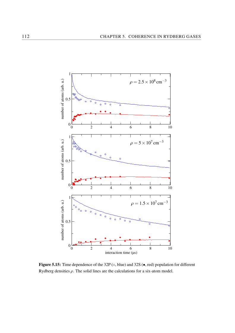
112 CHAPTER 5. COHERENCE IN RYDBERG GASES
0 2 4 6 8 100
0.5
1
num
ber
of
atom
s (a
rb. u.)
0 2 4 6 8 100
0.5
1
num
ber
of
atom
s (a
rb. u.)
0 2 4 6 8 10interaction time (µs)
0
0.5
1
num
ber
of
atom
s (a
rb. u.)
ρ= 2.5×108 cm−3
ρ= 5×107 cm−3
ρ= 1.5×107 cm−3
Figure 5.15: Time dependence of the 32P (, blue) and 32S (•, red) population for different
Rydberg densities ρ. The solid lines are the calculations for a six-atom model.
5.3. RESONANT ENERGY TRANSFER IN AN UNORDERED GAS 113
density measurement), and 1.5×107 cm−3 (low density measurement). These values are
reasonable considering a typical excitation fraction on the order of 10% for the highest
density. The spontaneous decay of the atoms is considered in the calculated curves by
multiplication with an exponential factor e−t/τeff . τeff is the effective lifetime of both
S and P states, estimated as τ−1eff = 1
2
(
(τS)−1 +(τP)
−1)
= (24µs)−1, where τS = 20µs
and τP = 30µs are calculated values for the lifetime of 32S and 32P states at vanishing
electric field. These values include both spontaneous decay and decay induced by black
body radiation [Gallagher, 1994]. The calculated curves for 32S shown in Fig. 5.15 are
scaled in height to the corresponding data, and the same scaling factor has been used
for the 32P curve of the same plot. The scaling factors differ for the three densities,
because of the difference in the absolute atom number and the saturation behavior of the
detector. Some redistribution to other Rydberg states may also take place and influence
the absolute number of Rydberg atoms detected [Walz-Flannigan et al., 2004]. The scale
of the plots is normalized to the calculated population fraction. Because of the different
temporal structure and the overlap of the field ionization signals of S and P states, a direct
comparison of the integrals is difficult. The restriction of the 32P integration window to
the narrow peak systematically underestimates the total atom number (See Fig. 5.15).
5.3.3 Effect of the interaction-induced motion of the atoms
As described in Chapter 4, the interaction-induced mechanical motion of the Rydberg
atoms can influence the system on a timescale of microseconds. It is therefore important
to estimate in how far the acceleration and possibly the collisional ionization of the atoms
play a role in the system described here. The collision time for two atoms on an attractive
dipole-dipole potential τdd has been calculated in Sec. 4.2 (see Eq. (4.7)). The atomic
motion should be expected to be negligible for the resonant energy transfer if the time
τdd exceeds the typical time scale of the s population rise time, τrise ≈ R30/C3 (as derived
above),
τdd
τrise
= 0.37
√
mRbC3
R0≫ 1 . (5.13)
Assuming C3 = (µµ′)/R3 ≈ 3× 10⁵ au and typical nearest-neighbor separations for den-
sities between 106 cm−3 and 108 cm−3, is is found that
τdd > 50τrise , (5.14)
114 CHAPTER 5. COHERENCE IN RYDBERG GASES
so that the motion of atoms should not have a significant influence on the initial time
development of the s population in the experimental configuration described here.
These estimations can be verified by including the motion of atoms in the model. The
interaction potential of two atoms is assumed to be a purely attractive,
V(R) = −µµ′
R3, (5.15)
and the Schrodinger equation for a two-atom system is solved for a time dependent inter-
action strength, as the distance R between the atoms changes with time according to the
classical equation of motion on the interaction potential (see Eq. (4.10)). As in the Monte
Carlo simulations presented in Sec. 4.3, the calculation is terminated once the distance of
the atoms becomes comparable to 4n2a0, the distance where collisional ionization hap-
pens with high probability. For a Rydberg density of 108 cm−3, the initial slope of the
s population is not affected when the motion of the atoms is included in the model, as
expected from (5.14). In addition to the variation of the interaction strength by the time-
dependent distance, the energy transfer dynamics will also be influenced by the presence
of free charges when ionizing collision have occurred. The electric field induced by a
free ion can shift surrounding atoms out of resonance. This influences the energy transfer
rates especially at longer delay times, where ions may have accumulated in the cloud. For
a Rydberg density of 108 cm−3, on the order of 5% of the atoms have collided after 10 µs
and, taking the nearest neighbor distribution for this density into account, each ion shifts
approximately one Rydberg atom out of resonance [Westermann, 2006]. The influence of
ions on the initial transfer rate is still negligible, as collisions occur only after several µs.
5.3.4 Coherent population oscillations of atom pairs
The observation of resonant energy transfer described so far assumed a completely un-
ordered gas of a given homogeneous density. If the sample could be prepared in a way
that only pairs of a specific distance are produced, coherent oscillations should become
visible. Such a sample could in principle be prepared by exploiting the long-range Ryd-
berg interactions. In a first step, a dilute Rydberg gas could be excited, and a second
(detuned) excitation laser could then excite partners to some of the Rydberg atoms at a
well-defined distance. A second approach to producing separated pairs at a given pair dis-
tance relies on first structuring the gas with micro-optical dipole traps and then exciting
a single Rydberg atom in each trap site exploiting the dipole blockade. Both techniques
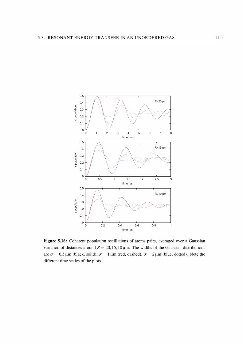
5.3. RESONANT ENERGY TRANSFER IN AN UNORDERED GAS 115
0
0.1
0.2
0.3
0.4
0.5
0 1 2 3 4 5 6 7 8
s p
op
ula
tio
n
time (µs)
R=20 µm
0
0.1
0.2
0.3
0.4
0.5
0 0.5 1 1.5 2 2.5 3
s p
opula
tion
time (µs)
R=15 µm
0
0.1
0.2
0.3
0.4
0.5
0 0.2 0.4 0.6 0.8 1
s p
opula
tion
time (µs)
R=10 µm
Figure 5.16: Coherent population oscillations of atoms pairs, averaged over a Gaussian
variation of distances around R = 20,15,10µm. The widths of the Gaussian distributions
are σ = 0.5µm (black, solid), σ = 1µm (red, dashed), σ = 2µm (blue, dotted). Note the
different time scales of the plots.
116 CHAPTER 5. COHERENCE IN RYDBERG GASES
will be considered for future experiments described in the Outlook (Chapter 6).
Fig. 5.16 shows a calculation of the expected population oscillations when a large
number of pairs oscillate simultaneously. The atoms are again prepared in the 32P state
and the population is transferred to S states via the energy transfer resonance (5.12). The
calculations are performed for three different mean values of the distance, R = 10µm,
R = 15µm, and R = 20µm. Residual fluctuations of the pair distance around different
mean values of R = 10µm, R = 15µm, and R = 20µm are accounted for by averaging
over 100 realizations with random variations of the distance according to a Gaussian
distribution with σ = 0.5µm (black, solid traces), σ = 1µm (red, dashed traces), and
σ = 2µm (blue, dotted traces). These results suggest that in order to observe coherent
oscillations, single Rydberg atoms or blockaded ensembles must be confined to a region
on the order of 1µm. Withσ= 2µm only a single oscillation is visible before the coherent
evolution is blurred by dephasing of the pairs, even at large interatomic distance of 20µm.
This should be kept in mind for the proposed experimental realization of energy transfer
in chains described in the following.
5.4 Energy transport in one-dimensional chains
A system of two coherently interacting Rydberg atoms could also be extended to a chain
of regularly arranged atoms, interacting with one another via dipole-dipole interactions.
If all atoms are prepared in the same Rydberg state except for one atom which is set to
another dipole-coupled state, the temporal evolution of this one excitation in the chain
can be studied. This mechanism is referred to as energy transport or exciton transport,
as the many-body state containing one excitation can be described as an exciton. Energy
transport plays a central role in many biological systems, such as the light-harvesting com-
plexes found in purple bacteria or photosynthesis in plants [Hader, 1999, Cogdell et al.,
2006, Ritz and Schulten, 2001]. In these systems, energy is picked up by a molecule ab-
sorbing light, and then transferred from one molecule to the next via dipole-coupling until
the excitation reaches a reaction center, where the energy can be converted. This process
has first been studied by Theodor Forster [Forster, 1948], and is frequently referred to as
Forster resonant energy transfer. Energy transport in molecular systems is extremely effi-
cient. This is one of the reasons why the exact mechanics of this process is being intensely
studied. Even single molecules of the light-harvesting system can now be isolated and in-
vestigated [Hofmann et al., 2004]. The question in how far this intermolecular energy
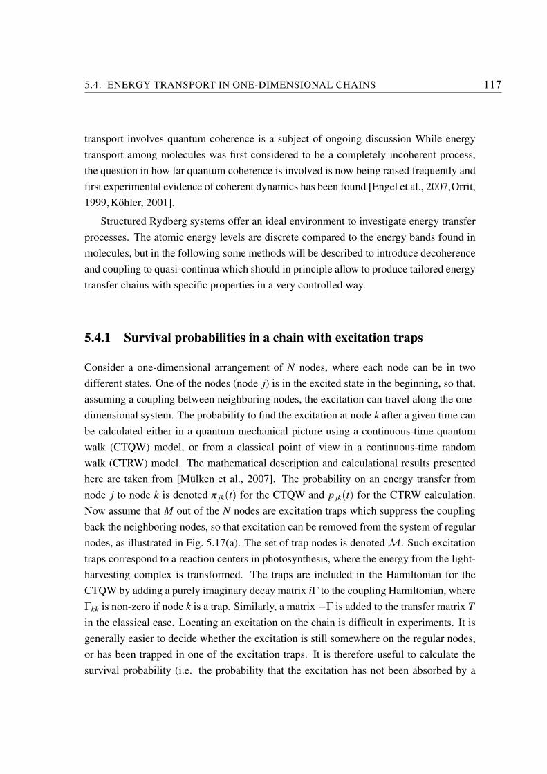
5.4. ENERGY TRANSPORT IN ONE-DIMENSIONAL CHAINS 117
transport involves quantum coherence is a subject of ongoing discussion While energy
transport among molecules was first considered to be a completely incoherent process,
the question in how far quantum coherence is involved is now being raised frequently and
first experimental evidence of coherent dynamics has been found [Engel et al., 2007,Orrit,
1999, Kohler, 2001].
Structured Rydberg systems offer an ideal environment to investigate energy transfer
processes. The atomic energy levels are discrete compared to the energy bands found in
molecules, but in the following some methods will be described to introduce decoherence
and coupling to quasi-continua which should in principle allow to produce tailored energy
transfer chains with specific properties in a very controlled way.
5.4.1 Survival probabilities in a chain with excitation traps
Consider a one-dimensional arrangement of N nodes, where each node can be in two
different states. One of the nodes (node j) is in the excited state in the beginning, so that,
assuming a coupling between neighboring nodes, the excitation can travel along the one-
dimensional system. The probability to find the excitation at node k after a given time can
be calculated either in a quantum mechanical picture using a continuous-time quantum
walk (CTQW) model, or from a classical point of view in a continuous-time random
walk (CTRW) model. The mathematical description and calculational results presented
here are taken from [Mulken et al., 2007]. The probability on an energy transfer from
node j to node k is denoted π jk(t) for the CTQW and p jk(t) for the CTRW calculation.
Now assume that M out of the N nodes are excitation traps which suppress the coupling
back the neighboring nodes, so that excitation can be removed from the system of regular
nodes, as illustrated in Fig. 5.17(a). The set of trap nodes is denoted M. Such excitation
traps correspond to a reaction centers in photosynthesis, where the energy from the light-
harvesting complex is transformed. The traps are included in the Hamiltonian for the
CTQW by adding a purely imaginary decay matrix iΓ to the coupling Hamiltonian, where
Γkk is non-zero if node k is a trap. Similarly, a matrix −Γ is added to the transfer matrix T
in the classical case. Locating an excitation on the chain is difficult in experiments. It is
generally easier to decide whether the excitation is still somewhere on the regular nodes,
or has been trapped in one of the excitation traps. It is therefore useful to calculate the
survival probability (i.e. the probability that the excitation has not been absorbed by a
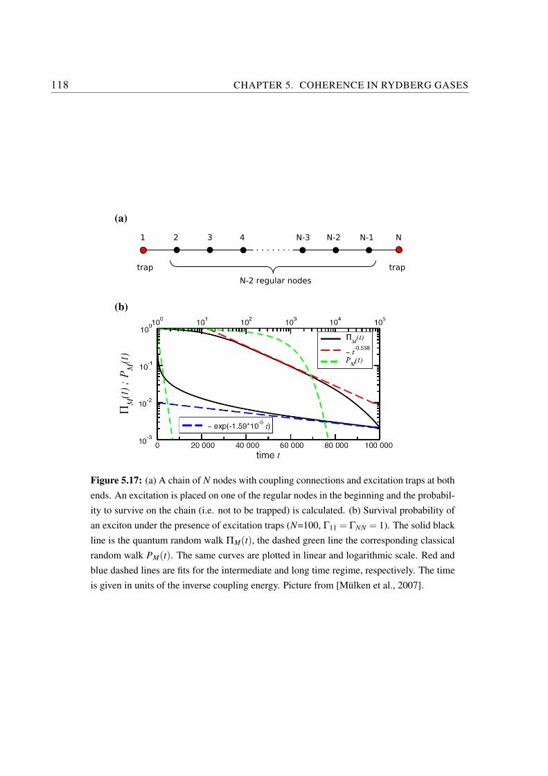
118 CHAPTER 5. COHERENCE IN RYDBERG GASES
(a)
N−2 regular nodes
trap trap
1 2 3 NN−1N−24 N−3
(b)
Figure 5.17: (a) A chain of N nodes with coupling connections and excitation traps at both
ends. An excitation is placed on one of the regular nodes in the beginning and the probabil-
ity to survive on the chain (i.e. not to be trapped) is calculated. (b) Survival probability of
an exciton under the presence of excitation traps (N=100, Γ11 = ΓNN = 1). The solid black
line is the quantum random walk ΠM(t), the dashed green line the corresponding classical
random walk PM(t). The same curves are plotted in linear and logarithmic scale. Red and
blue dashed lines are fits for the intermediate and long time regime, respectively. The time
is given in units of the inverse coupling energy. Picture from [Mulken et al., 2007].
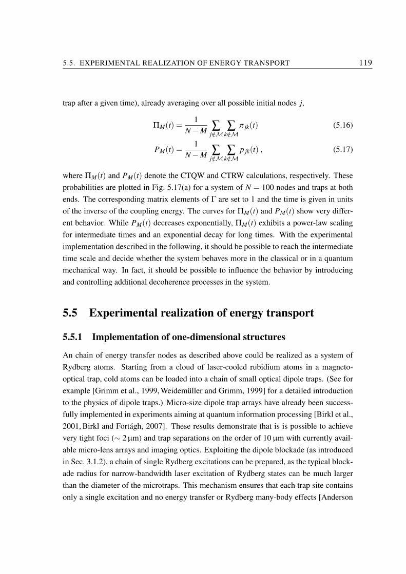
5.5. EXPERIMENTAL REALIZATION OF ENERGY TRANSPORT 119
trap after a given time), already averaging over all possible initial nodes j,
ΠM(t) =1
N−M∑j /∈M
∑k /∈M
π jk(t) (5.16)
PM(t) =1
N−M∑j /∈M
∑k /∈M
p jk(t) , (5.17)
where ΠM(t) and PM(t) denote the CTQW and CTRW calculations, respectively. These
probabilities are plotted in Fig. 5.17(a) for a system of N = 100 nodes and traps at both
ends. The corresponding matrix elements of Γ are set to 1 and the time is given in units
of the inverse of the coupling energy. The curves for ΠM(t) and PM(t) show very differ-
ent behavior. While PM(t) decreases exponentially, ΠM(t) exhibits a power-law scaling
for intermediate times and an exponential decay for long times. With the experimental
implementation described in the following, it should be possible to reach the intermediate
time scale and decide whether the system behaves more in the classical or in a quantum
mechanical way. In fact, it should be possible to influence the behavior by introducing
and controlling additional decoherence processes in the system.
5.5 Experimental realization of energy transport
5.5.1 Implementation of one-dimensional structures
An chain of energy transfer nodes as described above could be realized as a system of
Rydberg atoms. Starting from a cloud of laser-cooled rubidium atoms in a magneto-
optical trap, cold atoms can be loaded into a chain of small optical dipole traps. (See for
example [Grimm et al., 1999, Weidemuller and Grimm, 1999] for a detailed introduction
to the physics of dipole traps.) Micro-size dipole trap arrays have already been success-
fully implemented in experiments aiming at quantum information processing [Birkl et al.,
2001, Birkl and Fortagh, 2007]. These results demonstrate that is is possible to achieve
very tight foci (∼ 2µm) and trap separations on the order of 10 µm with currently avail-
able micro-lens arrays and imaging optics. Exploiting the dipole blockade (as introduced
in Sec. 3.1.2), a chain of single Rydberg excitations can be prepared, as the typical block-
ade radius for narrow-bandwidth laser excitation of Rydberg states can be much larger
than the diameter of the microtraps. This mechanism ensures that each trap site contains
only a single excitation and no energy transfer or Rydberg many-body effects [Anderson
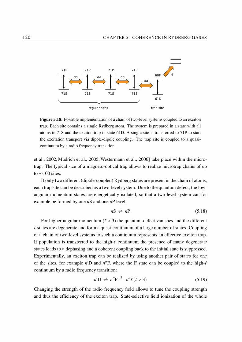
120 CHAPTER 5. COHERENCE IN RYDBERG GASES
71P 71P 71P 71P
71S 71S 71S 71S
60F
61D
rfdd dd dd
dd
regular sites trap site
Figure 5.18: Possible implementation of a chain of two-level systems coupled to an exciton
trap. Each site contains a single Rydberg atom. The system is prepared in a state with all
atoms in 71S and the exciton trap in state 61D. A single site is transferred to 71P to start
the excitation transport via dipole-dipole coupling. The trap site is coupled to a quasi-
continuum by a radio frequency transition.
et al., 2002, Mudrich et al., 2005, Westermann et al., 2006] take place within the micro-
trap. The typical size of a magneto-optical trap allows to realize microtrap chains of up
to ∼100 sites.
If only two different (dipole-coupled) Rydberg states are present in the chain of atoms,
each trap site can be described as a two-level system. Due to the quantum defect, the low-
angular momentum states are energetically isolated, so that a two-level system can for
example be formed by one nS and one nP level:
nS nP (5.18)
For higher angular momentum (ℓ > 3) the quantum defect vanishes and the different
ℓ states are degenerate and form a quasi-continuum of a large number of states. Coupling
of a chain of two-level systems to such a continuum represents an effective exciton trap.
If population is transferred to the high-ℓ continuum the presence of many degenerate
states leads to a dephasing and a coherent coupling back to the initial state is suppressed.
Experimentally, an exciton trap can be realized by using another pair of states for one
of the sites, for example n′D and n′′F, where the F state can be coupled to the high-ℓ
continuum by a radio frequency transition:
n′D n′′Frf−→ n′′ℓ (ℓ > 3) (5.19)
Changing the strength of the radio frequency field allows to tune the coupling strength
and thus the efficiency of the exciton trap. State-selective field ionization of the whole
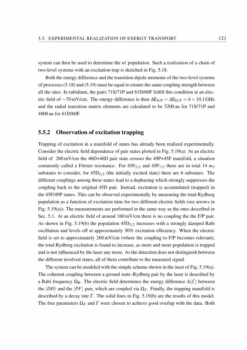
5.5. EXPERIMENTAL REALIZATION OF ENERGY TRANSPORT 121
system can then be used to determine the nℓ population. Such a realization of a chain of
two-level systems with an excitation trap is sketched in Fig. 5.18.
Both the energy difference and the transition dipole moments of the two-level systems
of processes (5.18) and (5.19) must be equal to ensure the same coupling strength between
all the sites. In rubidium, the pairs 71S/71P and 61D/60F fulfill this condition at an elec-
tric field of ∼70 mV/cm. The energy difference is then ∆ES/P = ∆ED/F = h× 10.1GHz
and the radial transition matrix elements are calculated to be 5200 au for 71S/71P and
4800 au for 61D/60F.
5.5.2 Observation of excitation trapping
Trapping of excitation in a manifold of states has already been realized experimentally.
Consider the electric field dependence of pair states plotted in Fig. 5.19(a). At an electric
field of 260 mV/cm the 46D+46D pair state crosses the 49P+45F manifold, a situation
commonly called a Forster resonance. For 45F5/2 and 45F7/2 there are in total 14 mJ
substates to consider, for 45D5/2 (the initially excited state) there are 6 substates. The
different couplings among these states lead to a dephasing which strongly suppresses the
coupling back to the original 45D pair. Instead, excitation is accumulated (trapped) in
the 45F/49P states. This can be observed experimentally by measuring the total Rydberg
population as a function of excitation time for two different electric fields (see arrows in
Fig. 5.19(a)). The measurements are performed in the same way as the ones described in
Sec. 5.1. At an electric field of around 160 mV/cm there is no coupling the the F/P pair.
As shown in Fig. 5.19(b) the population 45D5/2 increases with a strongly damped Rabi
oscillation and levels off at approximately 50% excitation efficiency. When the electric
field is set to approximately 260 mV/cm (where the coupling to F/P becomes relevant),
the total Rydberg excitation is found to increase, as more and more population is trapped
and is not influenced by the laser any more. As the detection does not distinguish between
the different involved states, all of them contribute to the measured signal.
The system can be modeled with the simple scheme shown in the inset of Fig. 5.19(a).
The coherent coupling between a ground state–Rydberg pair by the laser is described by
a Rabi frequency ΩR. The electric field determines the energy difference ∆(E) between
the |DD〉 and the |PF〉 pair, which are coupled via ΩF . Finally, the trapping manifold is
described by a decay rate Γ. The solid lines in Fig. 5.19(b) are the results of this model.
The free parameters ΩF and Γ were chosen to achieve good overlap with the data. Both
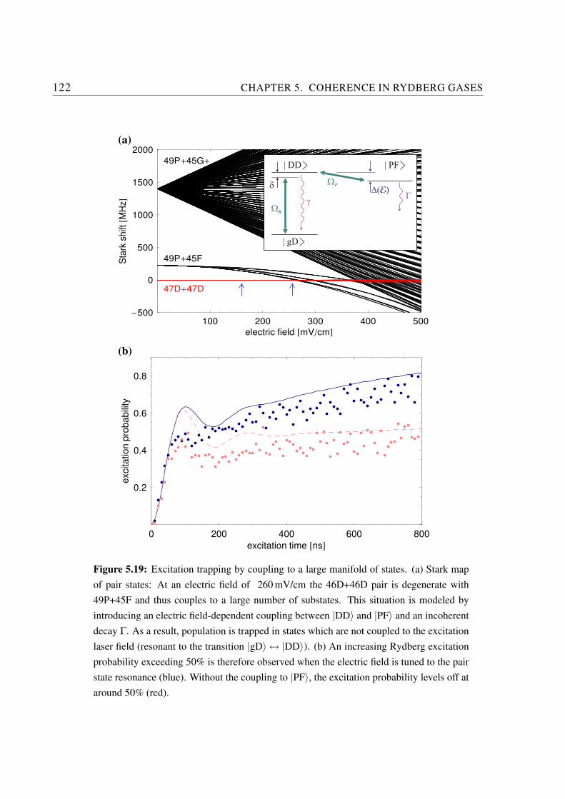
122 CHAPTER 5. COHERENCE IN RYDBERG GASES
(a)
100 200 300 400 500
electric field @mVcmD
-500
0
500
1000
1500
2000
Sta
rksh
ift@M
HzD
49P+45F
49P+45G+
47D+47D
WF
WR
D( )EG
g
| DD
| gD
| PF
d
(b)
0 200 400 600 800
excitation time @nsD
0.2
0.4
0.6
0.8
excita
tio
np
rob
ab
ility
Figure 5.19: Excitation trapping by coupling to a large manifold of states. (a) Stark map
of pair states: At an electric field of 260 mV/cm the 46D+46D pair is degenerate with
49P+45F and thus couples to a large number of substates. This situation is modeled by
introducing an electric field-dependent coupling between |DD〉 and |PF〉 and an incoherent
decay Γ. As a result, population is trapped in states which are not coupled to the excitation
laser field (resonant to the transition |gD〉 ↔ |DD〉). (b) An increasing Rydberg excitation
probability exceeding 50% is therefore observed when the electric field is tuned to the pair
state resonance (blue). Without the coupling to |PF〉, the excitation probability levels off at
around 50% (red).
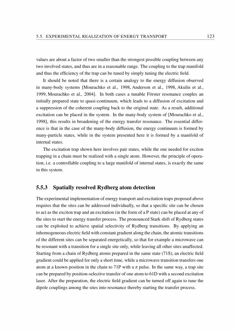
5.5. EXPERIMENTAL REALIZATION OF ENERGY TRANSPORT 123
values are about a factor of two smaller than the strongest possible coupling between any
two involved states, and thus are in a reasonable range. The coupling to the trap manifold
and thus the efficiency of the trap can be tuned by simply tuning the electric field.
It should be noted that there is a certain analogy to the energy diffusion observed
in many-body systems [Mourachko et al., 1998, Anderson et al., 1998, Akulin et al.,
1999, Mourachko et al., 2004]. In both cases a tunable Forster resonance couples an
initially prepared state to quasi-continuum, which leads to a diffusion of excitation and
a suppression of the coherent coupling back to the original state. As a result, additional
excitation can be placed in the system. In the many-body system of [Mourachko et al.,
1998], this results in broadening of the energy transfer resonance. The essential differ-
ence is that in the case of the many-body diffusion, the energy continuum is formed by
many-particle states, while in the system presented here it is formed by a manifold of
internal states.
The excitation trap shown here involves pair states, while the one needed for exciton
trapping in a chain must be realized with a single atom. However, the principle of opera-
tion, i.e. a controllable coupling to a large manifold of internal states, is exactly the same
in this system.
5.5.3 Spatially resolved Rydberg atom detection
The experimental implementation of energy transport and excitation traps proposed above
requires that the sites can be addressed individually, so that a specific site can be chosen
to act as the exciton trap and an excitation (in the form of a P state) can be placed at any of
the sites to start the energy transfer process. The pronounced Stark shift of Rydberg states
can be exploited to achieve spatial selectivity of Rydberg transitions. By applying an
inhomogeneous electric field with constant gradient along the chain, the atomic transitions
of the different sites can be separated energetically, so that for example a microwave can
be resonant with a transition for a single site only, while leaving all other sites unaffected.
Starting from a chain of Rydberg atoms prepared in the same state (71S), an electric field
gradient could be applied for only a short time, while a microwave transition transfers one
atom at a known position in the chain to 71P with a π pulse. In the same way, a trap site
can be prepared by position-selective transfer of one atom to 61D with a second excitation
laser. After the preparation, the electric field gradient can be turned off again to tune the
dipole couplings among the sites into resonance thereby starting the transfer process.
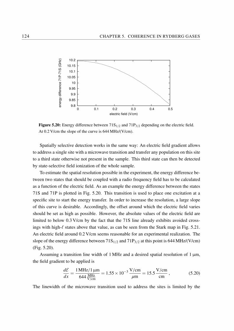
124 CHAPTER 5. COHERENCE IN RYDBERG GASES
9.8
9.85
9.9
9.95
10
10.05
10.1
10.15
10.2
0 0.1 0.2 0.3 0.4 0.5
en
erg
y d
iffe
ren
ce
71
P-7
1S
(G
Hz)
electric field (V/cm)
Figure 5.20: Energy difference between 71S1/2 and 71P3/2 depending on the electric field.
At 0.2 V/cm the slope of the curve is 644 MHz/(V/cm).
Spatially selective detection works in the same way: An electric field gradient allows
to address a single site with a microwave transition and transfer any population on this site
to a third state otherwise not present in the sample. This third state can then be detected
by state-selective field ionization of the whole sample.
To estimate the spatial resolution possible in the experiment, the energy difference be-
tween two states that should be coupled with a radio frequency field has to be calculated
as a function of the electric field. As an example the energy difference between the states
71S and 71P is plotted in Fig. 5.20. This transition is used to place one excitation at a
specific site to start the energy transfer. In order to increase the resolution, a large slope
of this curve is desirable. Accordingly, the offset around which the electric field varies
should be set as high as possible. However, the absolute values of the electric field are
limited to below 0.3 V/cm by the fact that the 71S line already exhibits avoided cross-
ings with high-ℓ states above that value, as can be seen from the Stark map in Fig. 5.21.
An electric field around 0.2 V/cm seems reasonable for an experimental realization. The
slope of the energy difference between 71S1/2 and 71P3/2 at this point is 644 MHz/(V/cm)
(Fig. 5.20).
Assuming a transition line width of 1 MHz and a desired spatial resolution of 1 µm,
the field gradient to be applied is
dEdx
=1MHz/1µm
644 MHzV/cm
= 1.55×10⁻³ V/cm
µm= 15.5
V/cm
cm, (5.20)
The linewidth of the microwave transition used to address the sites is limited by the
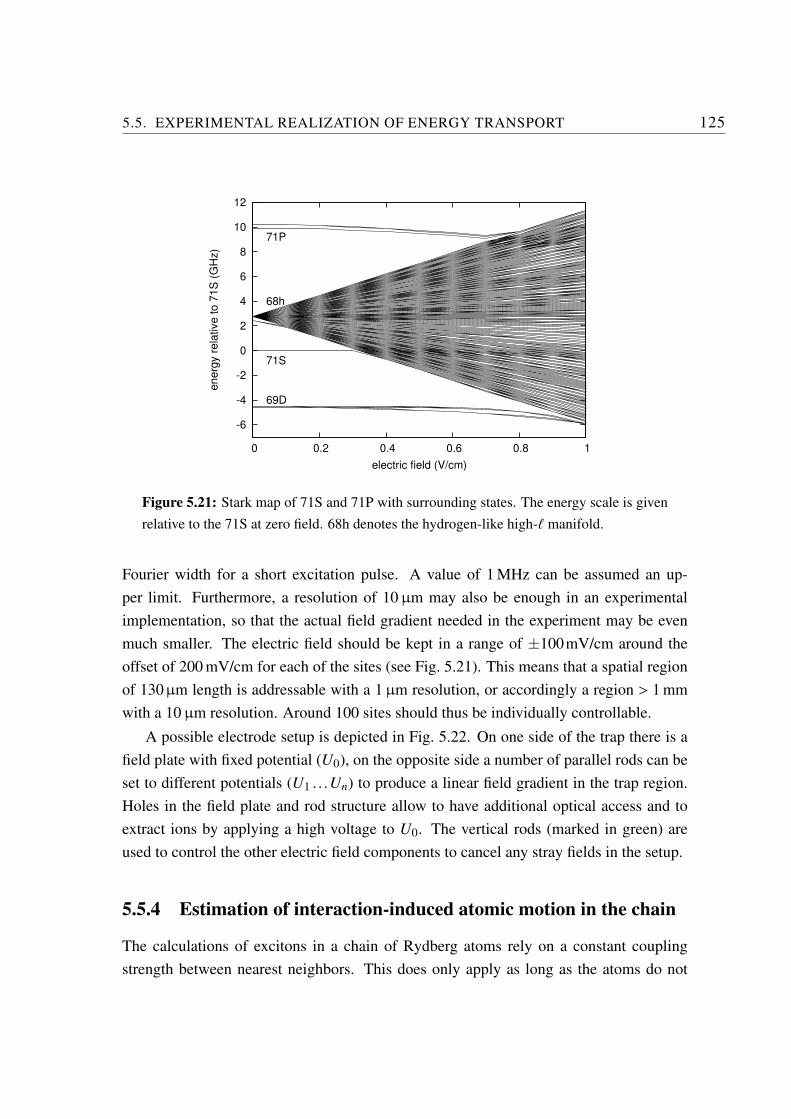
5.5. EXPERIMENTAL REALIZATION OF ENERGY TRANSPORT 125
-6
-4
-2
0
2
4
6
8
10
12
0 0.2 0.4 0.6 0.8 1
en
erg
y r
ela
tive
to
71
S (
GH
z)
electric field (V/cm)
71P
71S
69D
68h
Figure 5.21: Stark map of 71S and 71P with surrounding states. The energy scale is given
relative to the 71S at zero field. 68h denotes the hydrogen-like high-ℓ manifold.
Fourier width for a short excitation pulse. A value of 1 MHz can be assumed an up-
per limit. Furthermore, a resolution of 10 µm may also be enough in an experimental
implementation, so that the actual field gradient needed in the experiment may be even
much smaller. The electric field should be kept in a range of ±100mV/cm around the
offset of 200 mV/cm for each of the sites (see Fig. 5.21). This means that a spatial region
of 130µm length is addressable with a 1 µm resolution, or accordingly a region > 1 mm
with a 10 µm resolution. Around 100 sites should thus be individually controllable.
A possible electrode setup is depicted in Fig. 5.22. On one side of the trap there is a
field plate with fixed potential (U0), on the opposite side a number of parallel rods can be
set to different potentials (U1 . . .Un) to produce a linear field gradient in the trap region.
Holes in the field plate and rod structure allow to have additional optical access and to
extract ions by applying a high voltage to U0. The vertical rods (marked in green) are
used to control the other electric field components to cancel any stray fields in the setup.
5.5.4 Estimation of interaction-induced atomic motion in the chain
The calculations of excitons in a chain of Rydberg atoms rely on a constant coupling
strength between nearest neighbors. This does only apply as long as the atoms do not
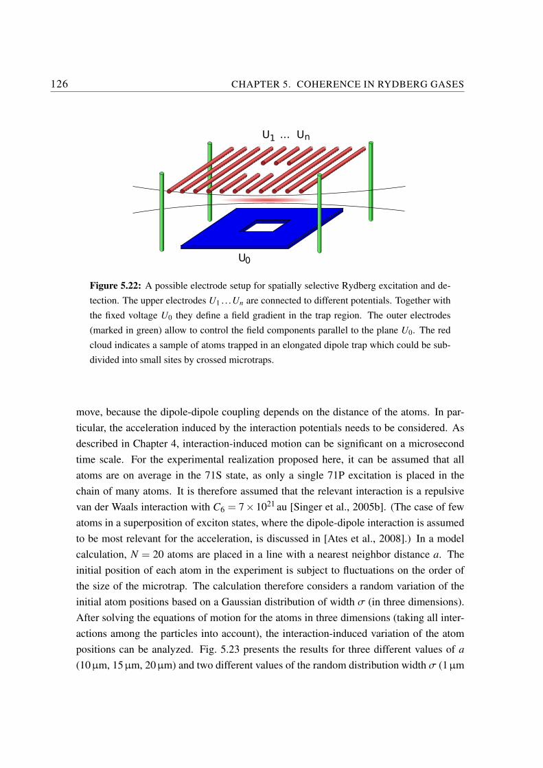
126 CHAPTER 5. COHERENCE IN RYDBERG GASES
Figure 5.22: A possible electrode setup for spatially selective Rydberg excitation and de-
tection. The upper electrodes U1 . . .Un are connected to different potentials. Together with
the fixed voltage U0 they define a field gradient in the trap region. The outer electrodes
(marked in green) allow to control the field components parallel to the plane U0. The red
cloud indicates a sample of atoms trapped in an elongated dipole trap which could be sub-
divided into small sites by crossed microtraps.
move, because the dipole-dipole coupling depends on the distance of the atoms. In par-
ticular, the acceleration induced by the interaction potentials needs to be considered. As
described in Chapter 4, interaction-induced motion can be significant on a microsecond
time scale. For the experimental realization proposed here, it can be assumed that all
atoms are on average in the 71S state, as only a single 71P excitation is placed in the
chain of many atoms. It is therefore assumed that the relevant interaction is a repulsive
van der Waals interaction with C6 = 7×10²¹ au [Singer et al., 2005b]. (The case of few
atoms in a superposition of exciton states, where the dipole-dipole interaction is assumed
to be most relevant for the acceleration, is discussed in [Ates et al., 2008].) In a model
calculation, N = 20 atoms are placed in a line with a nearest neighbor distance a. The
initial position of each atom in the experiment is subject to fluctuations on the order of
the size of the microtrap. The calculation therefore considers a random variation of the
initial atom positions based on a Gaussian distribution of width σ (in three dimensions).
After solving the equations of motion for the atoms in three dimensions (taking all inter-
actions among the particles into account), the interaction-induced variation of the atom
positions can be analyzed. Fig. 5.23 presents the results for three different values of a
(10µm, 15µm, 20µm) and two different values of the random distribution width σ (1µm
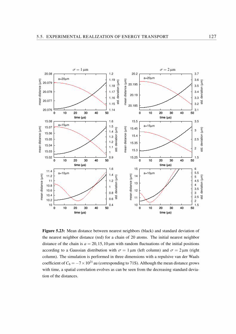
5.5. EXPERIMENTAL REALIZATION OF ENERGY TRANSPORT 127
σ= 1µm σ= 2µm
20.076
20.077
20.078
20.079
20.08
0 10 20 30 40 50
mean d
ista
nce (
µm
)
time (µs)
0 10 20 30 40 50 1.14
1.15
1.16
1.17
1.18
1.19
1.2
std
. devia
tion (
µm
)time (µs)
a=20µm
15.02
15.03
15.04
15.05
15.06
15.07
15.08
0 10 20 30 40 50
mean d
ista
nce (
µm
)
time (µs)
0 10 20 30 40 50 0.9
1
1.1
1.2
1.3
1.4
1.5
1.6
std
. devia
tion (
µm
)
time (µs)
a=15µm
10
10.2
10.4
10.6
10.8
11
11.2
11.4
0 10 20 30 40 50
mean d
ista
nce (
µm
)
time (µs)
0 10 20 30 40 50 0.4
0.6
0.8
1
1.2
1.4
1.6
std
. devia
tion (
µm
)
time (µs)
a=10µm
20.185
20.19
20.195
20.2
0 10 20 30 40 50
mean d
ista
nce (
µm
)
time (µs)
0 10 20 30 40 50 3.1
3.2
3.3
3.4
3.5
3.6
3.7
std
. devia
tion (
µm
)
time (µs)
a=20µm
15.25
15.3
15.35
15.4
15.45
15.5
0 10 20 30 40 50
mean d
ista
nce (
µm
)
time (µs)
0 10 20 30 40 50 1.5
2
2.5
3
3.5
std
. devia
tion (
µm
)
time (µs)
a=15µm
10
11
12
13
14
15
0 10 20 30 40 50
mean d
ista
nce (
µm
)
time (µs)
0 10 20 30 40 50 1.5
2
2.5
3
3.5
4
4.5
5
5.5
6
std
. devia
tion (
µm
)
time (µs)
a=10µm
Figure 5.23: Mean distance between nearest neighbors (black) and standard deviation of
the nearest neighbor distance (red) for a chain of 20 atoms. The initial nearest neighbor
distance of the chain is a = 20,15,10µm with random fluctuations of the initial positions
according to a Gaussian distribution with σ = 1µm (left column) and σ = 2µm (right
column). The simulation is performed in three dimensions with a repulsive van der Waals
coefficient ofC6 =−7×10²¹ au (corresponding to 71S). Although the mean distance grows
with time, a spatial correlation evolves as can be seen from the decreasing standard devia-
tion of the distances.
128 CHAPTER 5. COHERENCE IN RYDBERG GASES
and 2µm). The plots show the mean distance between nearest neighbors,
r = (N−1)−1N−1
∑i=1
|~ri+1 −~ri| , (5.21)
and the standard deviation of the nearest neighbor distance,
s =
√
√
√
√
1
N−1
N−1
∑i=1
(|~ri+1 −~ri|− r)2 , (5.22)
as functions of time. For initial separations of a = 20µm and a = 15µm, the motion
of the atoms is negligible. The change of the mean distance for a = 15µm and position
fluctuations of σ = 2µm, the mean nearest neighbor distance changes by only 1% over
a time of 50µs. At short initial distance (a = 10µm), motion can become significant.
For σ = 1µm, the mean distance rises by 10% over 50µs, for σ = 2µm, the increase
is already 50% at 40µs. Even though the repulsive forces increase the average distance
between the atoms, it also introduces a certain correlation of the atom positions and ef-
fectively decreases the disorder. This can be seen by the fact that the standard deviation
of the nearest neighbor distances s decreases with time. Its initial value is determined by
the random position fluctuations. Only after long delay times or for strong interactions
(a = 10µm) does the standard deviation increase again. The minimum of the standard
deviation corresponds to the peaking pair density discussed in Sec. 4.5 for a disordered
many-particle system.
The proposed implementation of resonant energy transfer mechanisms in a chain of
Rydberg atoms seems to be experimentally feasible. A planned realization of the setup is
expected to deliver first results in the near future, thereby opening the way to a new and
exciting application of ultracold Rydberg atoms.
Chapter 6
Conclusion and outlook
In this thesis different approaches to describing and controlling the many-particle dynam-
ics of interacting Rydberg gases have been discussed.
One part of this work focused on the interaction-induced motion, which always must
be considered in experiments involving Rydberg interactions. This mechanical motion of
the atoms can lead to unwanted decoherence and ionizing collisions. It has been found
that a Monte Carlo model of excitation and motion under the influence of long-range van
der Waals potentials can describe the early phase (several microseconds) of acceleration
and collisional ionization in the gas very well. Based on this description, information
about the Rydberg pair distribution and about the shape of the interaction potentials could
be extracted from experimental data. Collisional ionization has been identified as one
of the trigger processes for ultracold plasma formation and at the same time has been
utilized as a sensitive probe for variations in the distribution of Rydberg atom distances.
Different schemes of detuned excitation have been applied to influence the Rydberg atom
pair distribution and the collision dynamics.
In a second part, coherent processes in the excitation and the interaction of Rydberg
atoms have been studied. The control of excitation in terms of Rabi cycles is vital for the
implementation of quantum information processing schemes with Rydberg atoms. Direct
measurements and calculations of Rabi oscillations and Ramsey interference have been
presented. Despite the unordered arrangement of atoms in a gas, resonant energy pro-
cesses were successfully described in terms of a coherent few-body model, while a simple
two-atom model fails to reproduce the experimental observations. Coherent population
oscillations should be observable if atom pairs or chains are prepared with well-defined
129
130 CHAPTER 6. CONCLUSION AND OUTLOOK
interatomic distances. By deliberately introducing excitation traps or other sources of de-
phasing in such a structured system, the character of energy transfer dynamics (quantum
walk or classical random walk) can be influenced and observed. Experimental evidence
for excitation trapping in internal states has already been provided and a possible imple-
mentation of a spatially addressable regular chain for energy transfer studies has been
proposed.
Detailed knowledge of the different coherent and incoherent dynamic processes is
necessary to gain more control over ultracold Rydberg interactions and to further explore
the fascinating properties of ultracold Rydberg gases. The results of this thesis contribute
to this goal. The following projects for future research exemplify the broad range of
applications and the potential of these unique systems.
Rydbergmacrodimers The same long-range interactions which in this thesis have been
found to destabilize the system, may also, in some cases, provide stable long-range bound
states between the atoms [Boisseau et al., 2002]. In these so-called macrodimers, the re-
pulsive part of the interaction potential overtakes the attractive part already at distances
where the two electronic wavefunctions do not yet overlap. As a consequence, both atoms,
although bound, are still well separated and stable against collisions. (The stability can
be limited by autoionization through dipole-coupling, see Sec. 3.4.3.) Spectroscopic sig-
natures of molecular resonances have been observed at the crossing of long-range molec-
ular potentials [Farooqi et al., 2003, Stanojevic et al., 2006], and at shallow potential
minima at typical pair distances of magneto-optically trapped atoms [Schwettmann et al.,
2006, Overstreet et al., 2007]. Experimental evidence for bound long-range molecules
has not been provided so far. The results of this thesis suggest that it should be possi-
ble to prepare atom pairs at specific distances by detuned excitation. A first laser pulse
at the atomic resonance could excite a dilute gas of Rydberg atoms, while a second, far
detuned laser excites partners to some of the atoms at well-known distance. In order to
distinguish the additionally excited atoms from the bath of atoms prepared before, the ex-
citation lasers can address the two different isotopes of rubidium, so that the atoms can be
separated in the detection by time-of-flight techniques. For this purpose, a double-MOT
system is currently being set up to trap both isotopes simultaneously.
Rydberg–ground state molecules A second proposed class of molecules is the com-
bination of a Rydberg atom and one or more ground state atoms [Greene et al., 2000,
131
Granger et al., 2001, Hamilton et al., 2002, Liu and Rost, 2006]. The Born-Oppenheimer
potential curves describing the molecular potentials show a characteristic oscillatory be-
havior which is reminiscent of the Rydberg wavefunction, and the minima in these po-
tentials should support many vibrational states. Molecules formed from low angular mo-
mentum states (ℓ ≤ 2) are non-polar and have been identified as the cause for satellite
features in the spectra of hot Rydberg vapor [Greene et al., 2006]. Molecules involving
high angular momenta (ℓ≥ 3) exhibit an extraordinarily large dipole which is not found in
any other homonuclear molecules [Khuskivadze et al., 2002, Chibisov et al., 2002]. Due
to the shape of the electron density, these molecules are dubbed trilobite states.
Rydberg–ground state molecules can be formed when the electronic wavefunction
of the Rydberg atom extends all the way to the ground state atom. This requires much
higher densities than achieved with magneto-optical traps. Typical densities in Bose-
Einstein condensates are more appropriate. In a future setup, an optical dipole trap and
evaporation techniques will be implemented to achieve the necessary densities for the
observation of Rydberg–ground state molecular states.
Dense Rydberg gases Eventually increasing the density of the sample and lowering the
temperature will lead to the regime of Bose-Einstein condensation. Rydberg excitation
of a Bose-Einstein-condensed sample has recently be demonstrated [Heidemann et al.,
2008]. When superimposed with an optical lattice, the condensate can be turned into a
Mott insulator state, a perfectly filled lattice. Excitation of the atoms in this crystalline
structure may allow for the observation of delocalized electrons and metal-like properties.
Structured arrangements All the experiments presented here were performed in an
unordered atom cloud, so that coherent effects in the interaction were mostly concealed
by the random distribution of distances. For further studies of these effects, it is nec-
essary to impose a spatial structure on the sample, either by structuring the excitation
in the cloud, or by arranging the atoms in microtraps. Studies of spatial beam shaping
using an LCoS display are presented in Appendix B. As already mentioned in Sec, 5.4,
micro-optical lens arrays have already been successfully used by other groups to create ar-
rangements of tight laser foci of around 2µm waist [Birkl et al., 2001, Birkl and Fortagh,
2007]. This technique will be implemented in a future setup for Rydberg experiments.
Two-dimensional micro-lens arrays illuminated with two slightly tilted laser beams can
produce a collection of dipole trap pairs of variable distance. Provided that a total Ryd-
132 CHAPTER 6. CONCLUSION AND OUTLOOK
berg excitation blockade can be achieved in the traps, a large number of identical Rydberg
pairs can be prepared, ideally suited to investigate long-range binary interactions without
the influence of surrounding atoms. One-dimensional micro-lens arrangements may be
used as dipole-trap arrays to prepare a chain of regularly spaced Rydberg atoms, as pro-
posed in Sec. 5.4. The realization of this trap setup combined with the proposed spatially
resolved excitation and detection scheme is another goal for future experiments. As the
coupling between the atoms as well as the coupling of internal states can be controlled to
a high degree, such a setup can serve as a model system for different aspects of resonant
energy transport in tailored configurations.
Lifetimes and superradiance The lifetime of Rydberg states is not only determined
by the spontaneous decay to low-lying levels. Interaction with black-body radiation and
long-range interaction among the Rydberg atoms which lead to state redistribution and
ionization have substantial influence on the lifetime of a specific Rydberg state. Collec-
tive effects such as superradiance have also been found to play a role for the stability of
Rydberg gases and can decrease the lifetime of the states [Wang et al., 2007, Day et al.,
2008, Gounand et al., 1979]. Only few measurements of Rydberg lifetimes have been
performed so far (e.g. [Magalhaes et al., 2000, de Oliveira et al., 2002]). In a planned
future experiment the significance of superradiance for the redistribution of states will be
investigated and systematic measurements will help to disentangle the different effects
that contribute to the decay of Rydberg states.
Two-electron systems Instead of using alkali atoms with their single valence electron,
it is also of interest to study Rydberg states of atoms with two valence electrons, the al-
kaline earth metals. While in alkali atoms only one electron is available for trapping and
cooling, Rydberg interaction, and detection, two-electron atoms offer the possibility to
use one electron for Rydberg interaction and the other one for trapping or spectroscopy.
This technique has been successfully used to study ultracold plasmas in experiments with
strontium atoms [Simien et al., 2004]. Two-electron atoms thus allow to decouple inter-
actions and spatial control. Furthermore, doubly excited planetary atoms open the way to
a new area of fascinating Rydberg physics.
133
The realization of the above-mentioned projects is planned for the near future with a
technically improved experimental setup. Yet there are many more interesting applica-
tions which have to be tackled, such as the implementation of quantum gate operations.
And certainly there are even more fascinating aspects of the physics of ultracold Rydberg
atoms which still await to be discovered.

134 CHAPTER 6. CONCLUSION AND OUTLOOK
Appendix A
Three-level systems and Optical Bloch
Equations
Consider the three-level system depicted in Fig. A.1. The states |g〉, |e〉, and |r〉 corre-
spond to the ground state, the first excited state, and the Rydberg state, respectively. The
incident monochromatic light is described as a classical electric field,
~E(t) = ~E0,1 cos(ω1t)+ ~E0,2 cos(ω2t) , (A.1)
where ω1 and ω2 are the laser frequencies nearly resonant with the transitions |g〉 ↔ |e〉and |e〉 ↔ |r〉, respectively. Neglecting decay of the levels (i.e. the coupling to an infinite
number of initially empty modes of the electric field), the Hamiltonian can be expressed
as the sum of the atomic Hamiltonian HA and the coupling of the atomic dipole moment
~µ to the electric field,
H = HA−~µ~E(t) . (A.2)
The evolution of the density operator σ can now be derived from the Schrodinger equa-
tion:
ihd
dtσ= [HA−~µ~E(t),σ] (A.3)
The coupling to a quantum radiation field describing the spontaneous and black-body-
induced emission of the levels |e〉 and |r〉 can be introduced by adding damping terms with
the respective decay rates Γe and Γr. While the decay of the intermediate state |e〉 leads
back to the ground state |g〉, the state |r〉 is mainly transferred to nearby Rydberg states, so
that the population is removed from the three-level system. In the rotating wave approx-
imation, the Hamiltonian and the density matrix can be rewritten, effectively eliminating
135
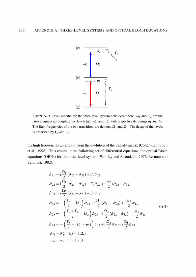
136 APPENDIX A. THREE-LEVEL SYSTEMS AND OPTICAL BLOCH EQUATIONS
|g〉
|e〉
|r〉
ω1
ω2
Ω1
Ω2
δ1
δ2
Γe
Γr
Figure A.1: Level scheme for the three-level system considered here. ω1 and ω2 are the
laser frequencies coupling the levels |g〉, |e〉, and |r〉, with respective detunings δ1 and δ2.
The Rabi frequencies of the two transitions are denoted Ω1 and Ω2. The decay of the levels
is described by Γe and Γr.
the high frequenciesω1 andω2 from the evolution of the density matrix [Cohen-Tannoudji
et al., 1998]. This results in the following set of differential equations, the optical Bloch
equations (OBEs) for the three-level system [Whitley and Stroud, Jr., 1976, Berman and
Salomaa, 1982]:
˙σ11 = iΩ1
2(σ12 − σ21)+Γe σ22
˙σ22 = iΩ1
2(σ21 − σ12)−Γe σ22 + i
Ω2
2(σ23 − σ32)
˙σ33 = iΩ2
2(σ32 − σ23)−Γr σ33
˙σ12 = −(
Γe
2− iδ1
)
σ12 + iΩ1
2(σ11 − σ22)+ i
Ω2
2σ13
˙σ23 = −(
Γe +Γr
2− iδ2
)
σ23 + iΩ2
2(σ22 − σ33)− i
Ω1
2σ13
˙σ13 = −(
Γr
2− i(δ1 +δ2)
)
σ13 + iΩ2
2σ12 − i
Ω1
2σ23
σi j = σ∗ji i, j = 1,2,3
σii = σii i = 1,2,3 .
(A.4)
137
Here δ1 = ωge−ω1 and δ2 = ωer−ω2 are the detunings of the laser frequencies from the
atomic transition frequencies. Ω1 and Ω2 denote the Rabi frequencies of the two tran-
sitions. In the experimental system the state |e〉 corresponds to 5P3/2 in 87Rb, with the
radiative lifetime δ1 = 2π×6.065 MHz [Steck, 2002]. The lifetime δ2 of the Rydberg state
|r〉 can be calculated according to [Gallagher, 1994], including the redistribution to other
Rydberg states induced by black-body radiation. In order to use the OBEs to describe
the excitation of Rydberg states as it is performed in the experiment, the Rabi frequencies
are themselves time-dependent, as the laser intensities are switched on and off. The exact
shape of the laser pulse can be measured with a fast photodiode and the rising and falling
edges can be approximated with error functions.
The eigenenergies of the three-level system can easily be calculated by diagonalizing
the interaction Hamiltonian, neglecting the radiative decay. In an atom–field basis, the
basis vectors are given by |g,N,n〉, |e,N− 1,n〉, |r,N− 1,n− 1〉, where N and n denote
the number of photons in the photon modes coupling the levels 1,2 and 2,3, respectively.
The corresponding Hamiltonian can then be written as
H = h
0 Ω1/2 0
Ω1/2 δ1 Ω2/2
0 Ω2/2 δ2
. (A.5)
Examples of eigenstates calculated by diagonalizing H can be found in Sec. 4.6.
For the case of a strong coupling of the lower transition and a weak upper laser
scanned over the resonance as a probe, The system exhibits the so-called Autler-Townes
splitting [Autler and Townes, 1955], which is of importance for some of the experiments
described in this thesis. In order to calculate the level splitting, it is sufficient to reduce
the system to the lower transition. In this case the remaining Hamiltonian reads
H′ = h
(
0 Ω1/2
Ω1/2 δ1
)
(A.6)
yielding the eigenvalues
E±/h =δ1
2±
√
(
δ1
2
)2
+
(
Ω1
2
)2
. (A.7)
138 APPENDIX A. THREE-LEVEL SYSTEMS AND OPTICAL BLOCH EQUATIONS
When the detuning from the lower transition is zero (δ1 = 0), the energies are given by
E± =hΩ1
2. (A.8)
The corresponding eigenstates are denoted
|±〉 =1√2
(|g〉± |e〉) . (A.9)
The splitting of the two lines visible in the excitation spectrum is thus equal to the Rabi
frequency Ω1, and the measured spectrum can be used to directly determine the Rabi
frequency of the lower transition. Using the complete description of the three-level system
given by the OBEs, even the upper Rabi frequency can be deduced from a comparison of
the measured spectrum with the calculation [Deiglmayr et al., 2006, Deiglmayr, 2006].
Appendix B
LCoS beam shaping
For many future experiments involving structured Rydberg gases it will be important to
generate small and controllable structures in the laser foci for structuring the excitation in
a cloud of atoms or for the implementation of small dipole traps. One approach of con-
trolling the shape and position of laser foci is the use of spatial light modulators (SLMs).
These devices usually consist of a liquid crystal display where each pixel induced a con-
trollable phase shift of the light reflected or transmitted. Being placed in the Fourier plane
of an imaging system, such devices can produce arbitrary intensity profiles. A liquid crys-
tal display can also act as a Fresnel lens, when the appropriate phase pattern is displayed.
For a sinosodial Fresnel zone pattern, the phase shift at a position x, y is given by
φ(x,y) =
(
1+ sin
(
2π
λ f(x2 + y2)
))
π , (B.1)
where λ is the wavelength of the light and f is the focal length of the Fresnel lens.
Beam shaping using a LCoS (liquid crystal on silicon) display has been successfully
demonstrated with the setup shown in Fig. B.1. The display device is used commercially
in video projectors. It has a resolution of 1280× 1024 pixels. A beam focus at a vari-
able distance can easily be obtained by projecting a Fresnel lens pattern on the display.
Unlike an image in a Fourier plane the position of this focus in the plane perpendicular
to the beam direction can be controlled by moving the pattern on the LCoS display. It
is even possible to produce a number of foci with given distances by simply adding the
corresponding Fresnel patterns.
The double lens pattern shown in Fig. B.2 is a superposition of two Fresnel zone pat-
139
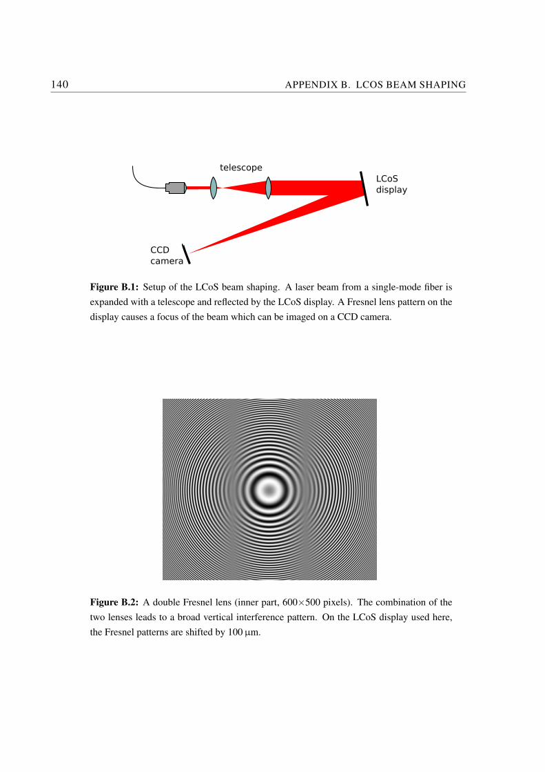
140 APPENDIX B. LCOS BEAM SHAPING
telescope
LCoS
display
CCD
camera
Figure B.1: Setup of the LCoS beam shaping. A laser beam from a single-mode fiber is
expanded with a telescope and reflected by the LCoS display. A Fresnel lens pattern on the
display causes a focus of the beam which can be imaged on a CCD camera.
Figure B.2: A double Fresnel lens (inner part, 600×500 pixels). The combination of the
two lenses leads to a broad vertical interference pattern. On the LCoS display used here,
the Fresnel patterns are shifted by 100 µm.
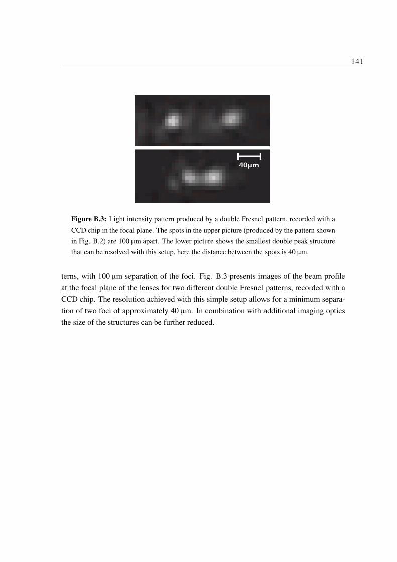
141
Figure B.3: Light intensity pattern produced by a double Fresnel pattern, recorded with a
CCD chip in the focal plane. The spots in the upper picture (produced by the pattern shown
in Fig. B.2) are 100 µm apart. The lower picture shows the smallest double peak structure
that can be resolved with this setup, here the distance between the spots is 40 µm.
terns, with 100 µm separation of the foci. Fig. B.3 presents images of the beam profile
at the focal plane of the lenses for two different double Fresnel patterns, recorded with a
CCD chip. The resolution achieved with this simple setup allows for a minimum separa-
tion of two foci of approximately 40 µm. In combination with additional imaging optics
the size of the structures can be further reduced.

142 APPENDIX B. LCOS BEAM SHAPING
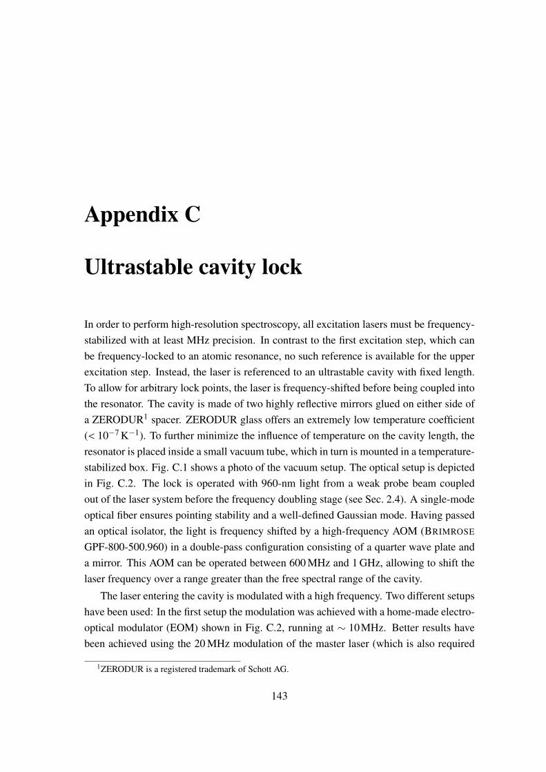
Appendix C
Ultrastable cavity lock
In order to perform high-resolution spectroscopy, all excitation lasers must be frequency-
stabilized with at least MHz precision. In contrast to the first excitation step, which can
be frequency-locked to an atomic resonance, no such reference is available for the upper
excitation step. Instead, the laser is referenced to an ultrastable cavity with fixed length.
To allow for arbitrary lock points, the laser is frequency-shifted before being coupled into
the resonator. The cavity is made of two highly reflective mirrors glued on either side of
a ZERODUR1 spacer. ZERODUR glass offers an extremely low temperature coefficient
(< 10−7 K−1). To further minimize the influence of temperature on the cavity length, the
resonator is placed inside a small vacuum tube, which in turn is mounted in a temperature-
stabilized box. Fig. C.1 shows a photo of the vacuum setup. The optical setup is depicted
in Fig. C.2. The lock is operated with 960-nm light from a weak probe beam coupled
out of the laser system before the frequency doubling stage (see Sec. 2.4). A single-mode
optical fiber ensures pointing stability and a well-defined Gaussian mode. Having passed
an optical isolator, the light is frequency shifted by a high-frequency AOM (BRIMROSE
GPF-800-500.960) in a double-pass configuration consisting of a quarter wave plate and
a mirror. This AOM can be operated between 600 MHz and 1 GHz, allowing to shift the
laser frequency over a range greater than the free spectral range of the cavity.
The laser entering the cavity is modulated with a high frequency. Two different setups
have been used: In the first setup the modulation was achieved with a home-made electro-
optical modulator (EOM) shown in Fig. C.2, running at ∼ 10MHz. Better results have
been achieved using the 20 MHz modulation of the master laser (which is also required
1ZERODUR is a registered trademark of Schott AG.
143
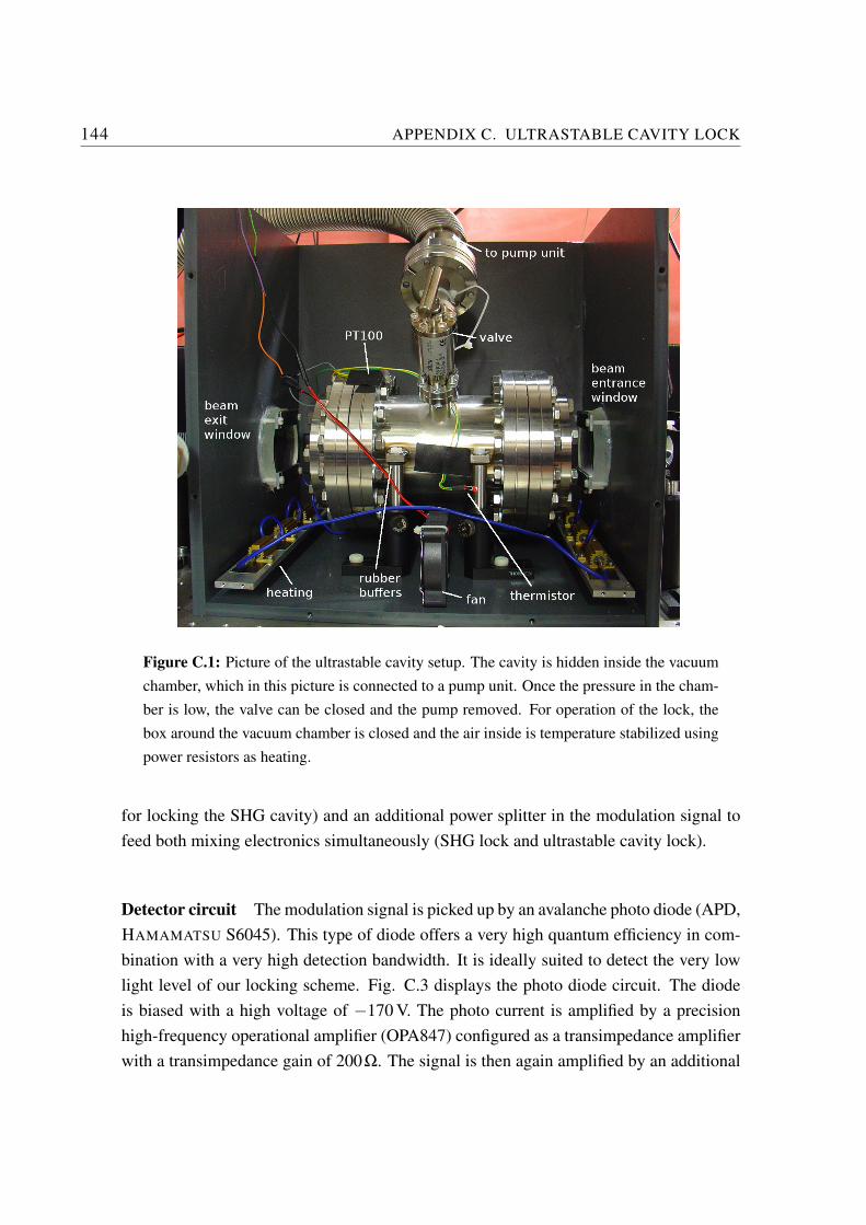
144 APPENDIX C. ULTRASTABLE CAVITY LOCK
Figure C.1: Picture of the ultrastable cavity setup. The cavity is hidden inside the vacuum
chamber, which in this picture is connected to a pump unit. Once the pressure in the cham-
ber is low, the valve can be closed and the pump removed. For operation of the lock, the
box around the vacuum chamber is closed and the air inside is temperature stabilized using
power resistors as heating.
for locking the SHG cavity) and an additional power splitter in the modulation signal to
feed both mixing electronics simultaneously (SHG lock and ultrastable cavity lock).
Detector circuit The modulation signal is picked up by an avalanche photo diode (APD,
HAMAMATSU S6045). This type of diode offers a very high quantum efficiency in com-
bination with a very high detection bandwidth. It is ideally suited to detect the very low
light level of our locking scheme. Fig. C.3 displays the photo diode circuit. The diode
is biased with a high voltage of −170 V. The photo current is amplified by a precision
high-frequency operational amplifier (OPA847) configured as a transimpedance amplifier
with a transimpedance gain of 200Ω. The signal is then again amplified by an additional
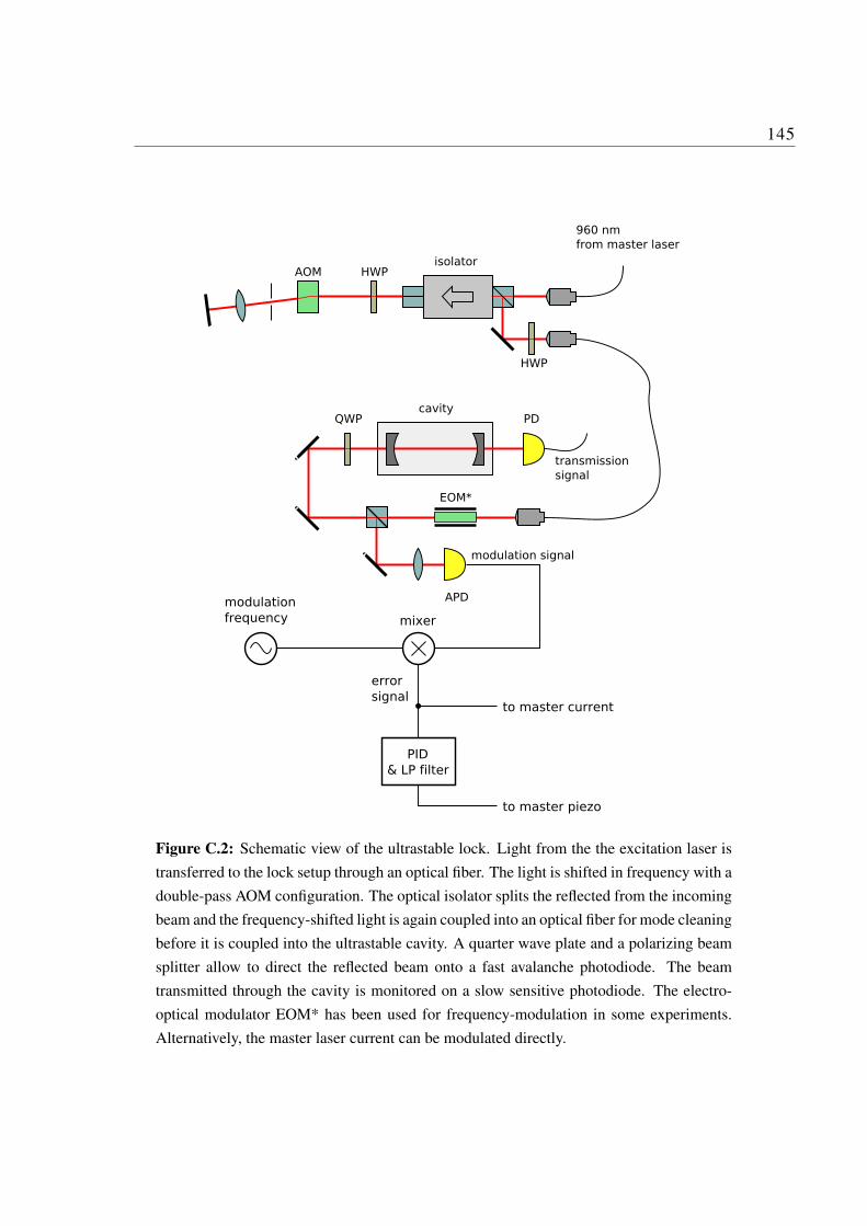
145
960 nm
from master laser
QWPcavity
PD
APD
isolatorHWPAOM
HWP
modulation signal
transmission
signal
EOM*
modulation
frequency mixer
error
signal
PID
& LP filter
to master piezo
to master current
Figure C.2: Schematic view of the ultrastable lock. Light from the the excitation laser is
transferred to the lock setup through an optical fiber. The light is shifted in frequency with a
double-pass AOM configuration. The optical isolator splits the reflected from the incoming
beam and the frequency-shifted light is again coupled into an optical fiber for mode cleaning
before it is coupled into the ultrastable cavity. A quarter wave plate and a polarizing beam
splitter allow to direct the reflected beam onto a fast avalanche photodiode. The beam
transmitted through the cavity is monitored on a slow sensitive photodiode. The electro-
optical modulator EOM* has been used for frequency-modulation in some experiments.
Alternatively, the master laser current can be modulated directly.
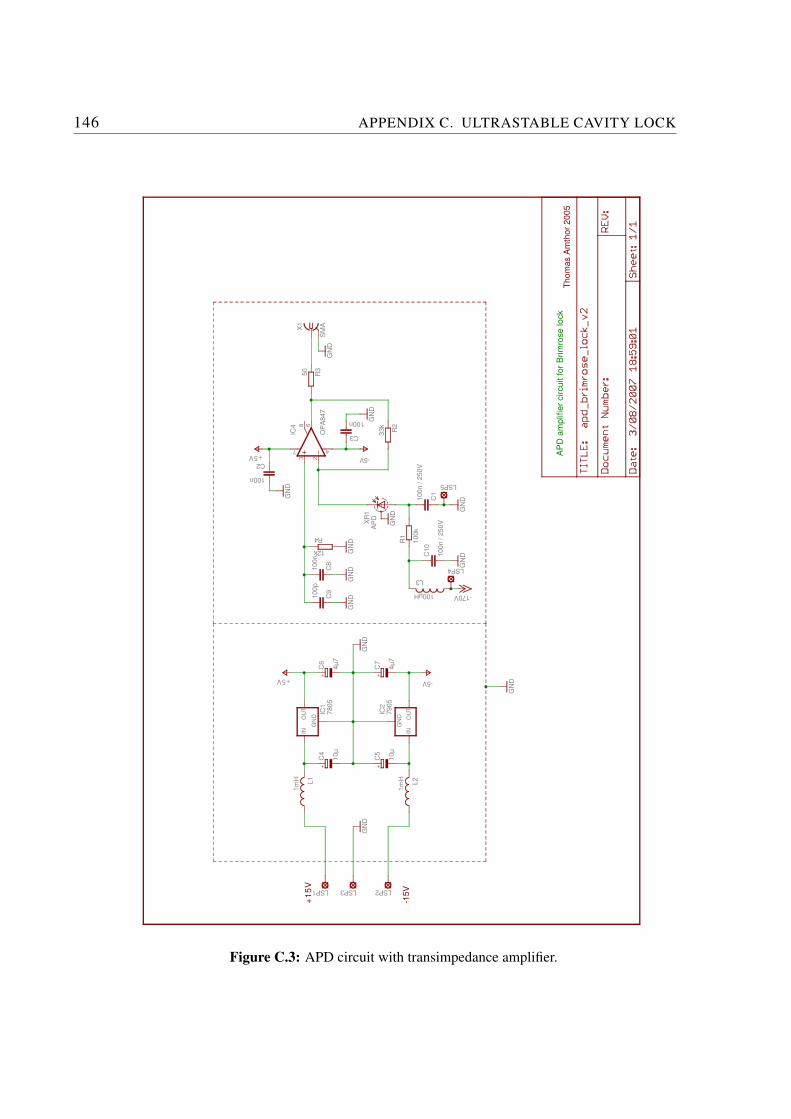
146 APPENDIX C. ULTRASTABLE CAVITY LOCK
AP
D a
mp
lifie
r c
irc
uit
fo
r B
rim
ros
e l
oc
kT
ho
ma
s A
mth
or
20
05
+1
5V
-15
V
+ +
+ +
R1
R2
C1
C2
C3
X1
L1
L2
C4
C5
C6
C7
LSP1 LSP2LSP3
R3
R4
C8
C9
8
236
IC4
7 4
L3
C1
0
LSP4
LSP5
XR
1
IC1
GN
D
INO
UT
IC2
GN
D OU
TIN
10
0k
33
k
10
0n
/ 2
50
V
GN
D
-170V
GN
D
100n
100n
+5V -5V
GN
D
GN
D
SM
AG
ND
1m
H
1m
H
10
µ
10
µ
4µ
7
4µ
7
-5V+5V
GN
DG
ND
GN
D
50
12k
10
0n
10
0p
GN
DG
ND
OP
A8
47
100µH
10
0n
/ 2
50
V
GN
D
AP
D
GN
D
78
05
79
05
Figure C.3: APD circuit with transimpedance amplifier.
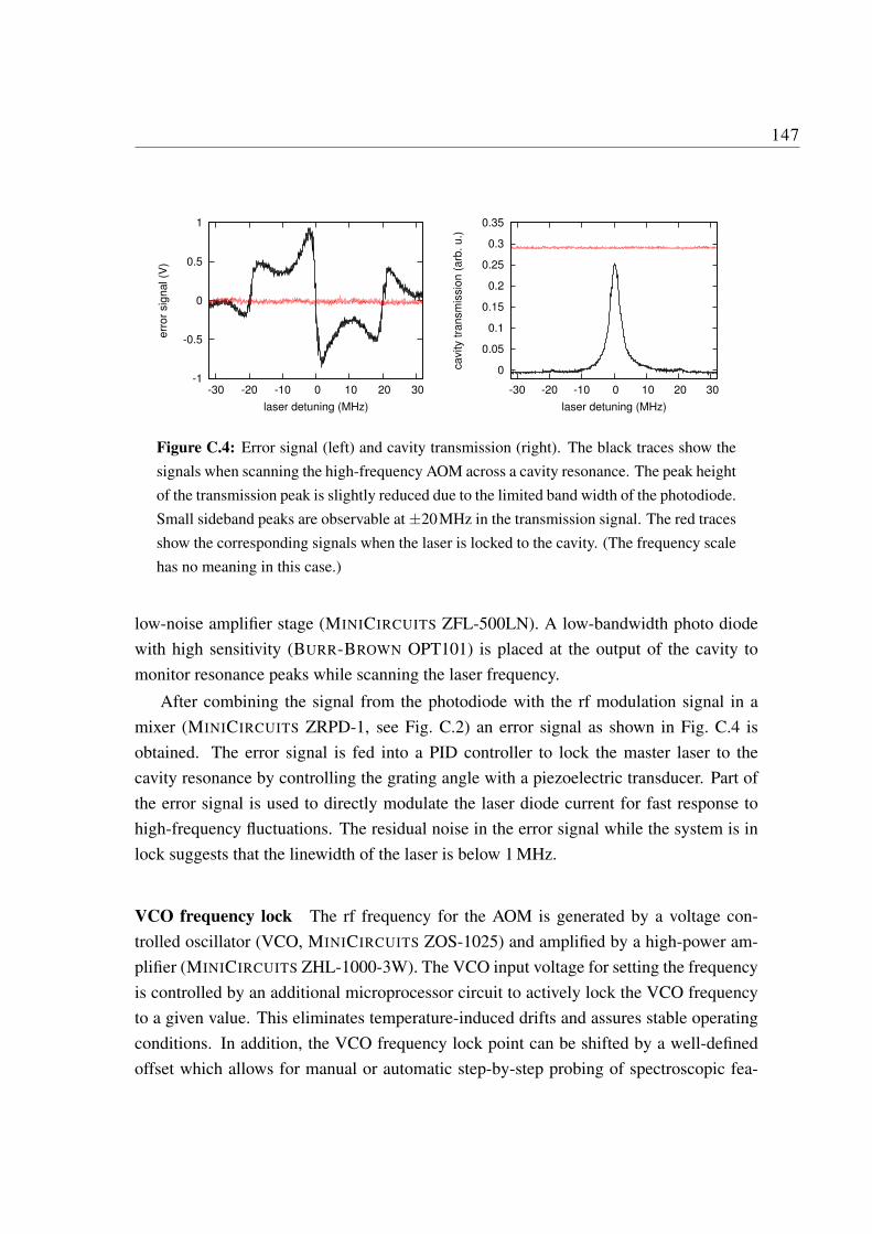
147
-1
-0.5
0
0.5
1
-30 -20 -10 0 10 20 30
err
or
sig
na
l (V
)
laser detuning (MHz)
0
0.05
0.1
0.15
0.2
0.25
0.3
0.35
-30 -20 -10 0 10 20 30
ca
vity t
ran
sm
issio
n (
arb
. u
.)
laser detuning (MHz)
Figure C.4: Error signal (left) and cavity transmission (right). The black traces show the
signals when scanning the high-frequency AOM across a cavity resonance. The peak height
of the transmission peak is slightly reduced due to the limited band width of the photodiode.
Small sideband peaks are observable at ±20MHz in the transmission signal. The red traces
show the corresponding signals when the laser is locked to the cavity. (The frequency scale
has no meaning in this case.)
low-noise amplifier stage (MINICIRCUITS ZFL-500LN). A low-bandwidth photo diode
with high sensitivity (BURR-BROWN OPT101) is placed at the output of the cavity to
monitor resonance peaks while scanning the laser frequency.
After combining the signal from the photodiode with the rf modulation signal in a
mixer (MINICIRCUITS ZRPD-1, see Fig. C.2) an error signal as shown in Fig. C.4 is
obtained. The error signal is fed into a PID controller to lock the master laser to the
cavity resonance by controlling the grating angle with a piezoelectric transducer. Part of
the error signal is used to directly modulate the laser diode current for fast response to
high-frequency fluctuations. The residual noise in the error signal while the system is in
lock suggests that the linewidth of the laser is below 1 MHz.
VCO frequency lock The rf frequency for the AOM is generated by a voltage con-
trolled oscillator (VCO, MINICIRCUITS ZOS-1025) and amplified by a high-power am-
plifier (MINICIRCUITS ZHL-1000-3W). The VCO input voltage for setting the frequency
is controlled by an additional microprocessor circuit to actively lock the VCO frequency
to a given value. This eliminates temperature-induced drifts and assures stable operating
conditions. In addition, the VCO frequency lock point can be shifted by a well-defined
offset which allows for manual or automatic step-by-step probing of spectroscopic fea-
148 APPENDIX C. ULTRASTABLE CAVITY LOCK
tures. The microcontroller circuit is shown in Fig. C.5. A commercial frequency counter
(HAMEG HM 8021-3) is used to determine the VCO output frequency and a microcon-
troller (ATMEL ATmega8515) compares the result to a set value. A correction to the VCO
control voltage is then generated by a digital-to-analog converter (DAC912) and added to
the input voltage by an operational amplifier. As the frequency counter does not feature
a digital output, the displayed value is read out directly by listening to the internal serial
data line of the LED display. The behavior of the lock circuit is fully software-controlled.
Different software versions are available to incorporate different functions and configu-
rations of the input lines and buttons. A 16-character LCD display driven by the same
processor provides information about the status of the lock. Depending on the software
version used, the VCO lock offers the following features:
• Lock point hold: The current control output voltage can be held constant without
reacting to changes of the VCO frequency. In this way a frequency scan can be per-
formed by an external ramp generator and the lock point can be retrieved afterwards
by releasing the hold function.
• Lock point shift: Two buttons allow to shift the lockpoint in pre-defined steps. This
feature is useful when the detuning from an atomic resonance should be varied in a
well-defined way.
• Lock point switching: A TTL input signal can be used to switch the lockpoint
frequency by a pre-defined amount, for example to toggle automatically between
two detunings.
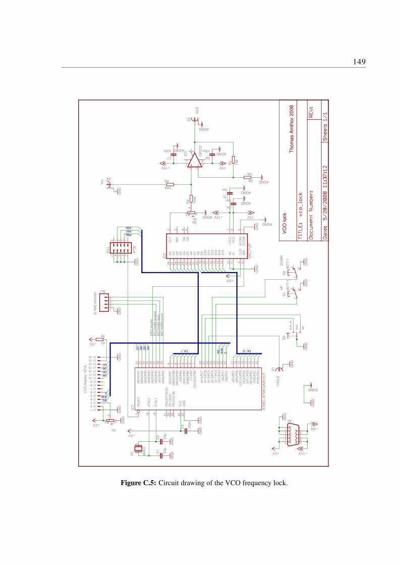
149
D0..7 D8..15
ER/W
RS
Q4
Q5
Q6
Q7
E
R/W
RS
Q4
Q5
Q6
Q7
PB7
PB6
PB5
VC
O l
oc
k
Th
om
as
Am
tho
r 2
00
8
D0
28
D1
27
D2
26
D3
25
D4
24
D5
23
D6
22
D7
21
D8
20
D9
19
D1
01
8
D1
11
7
D1
21
6
D1
31
5
D1
41
4
A0
12
A1
11
CL
R\
9
WR
\1
0
OU
T3
RE
F5
DC
OM
1A
CO
M2
-VC
C8
+V
CC
7
OA
4
GA
6
D1
51
3
IC2
8
1
236
5
IC3
7 4
X1
X2
162738495
X3
1234
SL1
AE
S
R1
AE
S
R2
21
S1
32
1
S2
3
X4
(AD
7)P
A7
32
(AD
6)P
A6
33
(AD
5)P
A5
34
(AD
4)P
A4
35
(AD
3)P
A3
36
(AD
2)P
A2
37
(AD
1)P
A1
38
(AD
0)P
A0
39
(SC
K)P
B7
8
(MIS
O)P
B6
7
(MO
SI)
PB
56
(SS
)PB
45
(AIN
1)P
B3
4
(AIN
0)P
B2
3
(T1
)PB
12
(T0
/OC
0)P
B0
1
(A1
5)P
C7
28
(A1
4)P
C6
27
(A1
3)P
C5
26
(A1
2)P
C4
25
(A1
1)P
C3
24
(A1
0)P
C2
23
(A9
)PC
12
2
(A8
)PC
02
1
PE
2(O
C1
B)
29
PE
1(A
LE
)3
0P
E0
(IC
P/I
NT
2)
31
XT
AL
11
9
XT
AL
21
8
VC
C4
0
GN
D2
0
RE
SE
T9
(RX
D)P
D0
10
(TX
D)P
D1
11
(IN
T0
)PD
21
2(I
NT
1)P
D3
13
(XC
K)P
D4
14
(OC
1A
)PD
51
5(W
R)P
D6
16
(RD
)PD
71
7
IC1
C1
C2
C3
C4
C5
21
Q1
R3
R4
R5 R6
R7
C6C7
J1-1J1-2J1-3J1-4J1-5J1-6J1-7J1-8J1-9J1-10J1-11J1-12J1-13J1-14J1-15J1-16
135
24679
SV
1
810
se
t
loc
k
loc
k o
ff
S3
MC
14
48
9 e
na
ble
MC
14
48
9 d
ata
MC
14
48
9 c
loc
k
DA
C s
tro
be
UP
DO
WND
AC
71
2P
OP
27
Z
HO
LD
Vo
ut
to f
req
co
un
ter
5k
90
77
-19
07
7-1
Vin
AT
ME
L A
TM
EG
A8
51
5-P
GN
D
GN
DG
ND
33
p3
3p
10
0n
10n
10n
GN
D
GN
DG
ND
4M
Hz
GN
D
10
k
10
0k
100k
10k
39
AGND
AGND
AGND
AGND
100n100n
AGND
+5V
+5V
GN
D
+15V
+15V
-15V
-15V
AGNDAGND
GN
D
AGND
GN
D
GN
D
AGND
GN
D
+5V +15V
-15V
GN
D
LC
D d
isp
lay
16
1A
GN
D
+5V GN
DG
ND
+5V
pro
gG
ND
GN
D
Figure C.5: Circuit drawing of the VCO frequency lock.

150 APPENDIX C. ULTRASTABLE CAVITY LOCK
Appendix D
Electronic circuits
A number of electronic apparatus have been developed in the course of this work, some
of which are presented here:
In Sec. D.1 the high-speed discriminator used to count single ion events is described.
Its application in the experimental setup can be found in Sec. 2.4.
A device for heating vacuum chambers in a controlled way is presented in Sec. D.2. It
is software-controlled and features a 8×8 coupling matrix of sensors and heating outputs.
Sec. D.3 describes a low-cost precision wavelength sensor based on a double photo-
diode structure.
151
152 APPENDIX D. ELECTRONIC CIRCUITS
D.1 High-speed pulse discriminator
The detection of single ions requires a very sensitive and fast comparator circuit to dis-
criminate single pulses from the microchannel plate (MCP) detector.
The circuit is depicted in Fig. D.1. It consists mainly of an inverting buffer amplifier
and a high-speed comparator. The amplifier section is built with a wideband precision op-
erational amplifier (BURR-BROWN OPA656). It converts the negative input pulses from
the MCP to positive pulses suitable for the unipolar comparator. A Schottky diode D2
clips off any remaining negative overshoots and the resistors R4/R6 shift the amplified
signal by an offset of some mV to ensure a positive comparator input. The discrimina-
tor level can be set with potentiometer R7. The high-speed comparator (BURR-BROWN
TLV3501) has an output rise time of only 1.5 ns. IC2 (74LS541) is a TTL buffer to drive
additional circuits connected to the output of this device. The additional capacitors have
been carefully chosen to eliminate oscillatory behavior and ringing while preserving a
high bandwidth. The comparator circuit is able to discriminate negative input pulses of
only a few mV pulse hight and a few ns width. A detected input pulse results in a TTL
(high) output pulse to be further processed or counted.
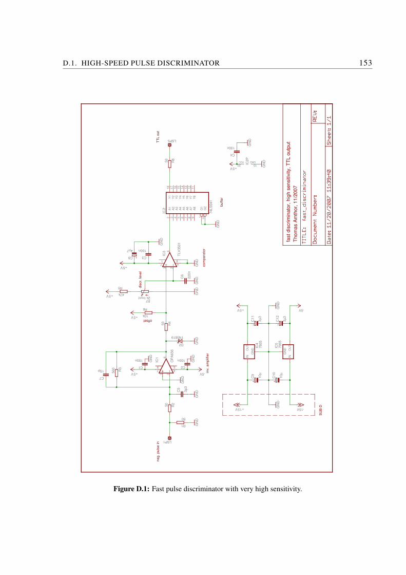
D.1. HIGH-SPEED PULSE DISCRIMINATOR 153
fast discriminator, high sensitivity, TTL output
Thomas Amthor, 11/2007
SUB-D
discr. level
inv. amplifier
comparator
buffer
neg. pulse in
TTL out
offset
+
+ +
+ +
8
236
5
IC1
7 4C1 C2
C3
C4
C5
C6
R1
R2
R3
R4
C7
8
23
1
6
IC3
7 4
LSP1
LSP5
R5
R6
D2
C8
G1
1
A1
2
A2
3
A3
4
A4
5
A5
6
A6
7
A7
8
A8
9Y8
11
Y7
12
Y6
13
Y5
14
Y4
15
Y3
16
Y2
17
Y1
18
G2
19
1020 IC2P
GNDVCC
IC4
GND
INOUT
IC5
GND OUT
IN
C9
C10
C11
C12R7
R8
OPA656
100n 100n
100n
100n
3p3
220n
50
50
560
50
15p
GND
GND
GND
GND
GND
GND
GND
GND
GND
+5V
+5V
+5V
-5V
TLV3501
GND
GND
+5V 47k
10k+5V
1N5819
4µ7
74LS541
GND
7805
7905
10µ
10µ
3µ3
3µ3
GND
-5V+5V
+15V -15VGND
2k front
GND
50
Figure D.1: Fast pulse discriminator with very high sensitivity.
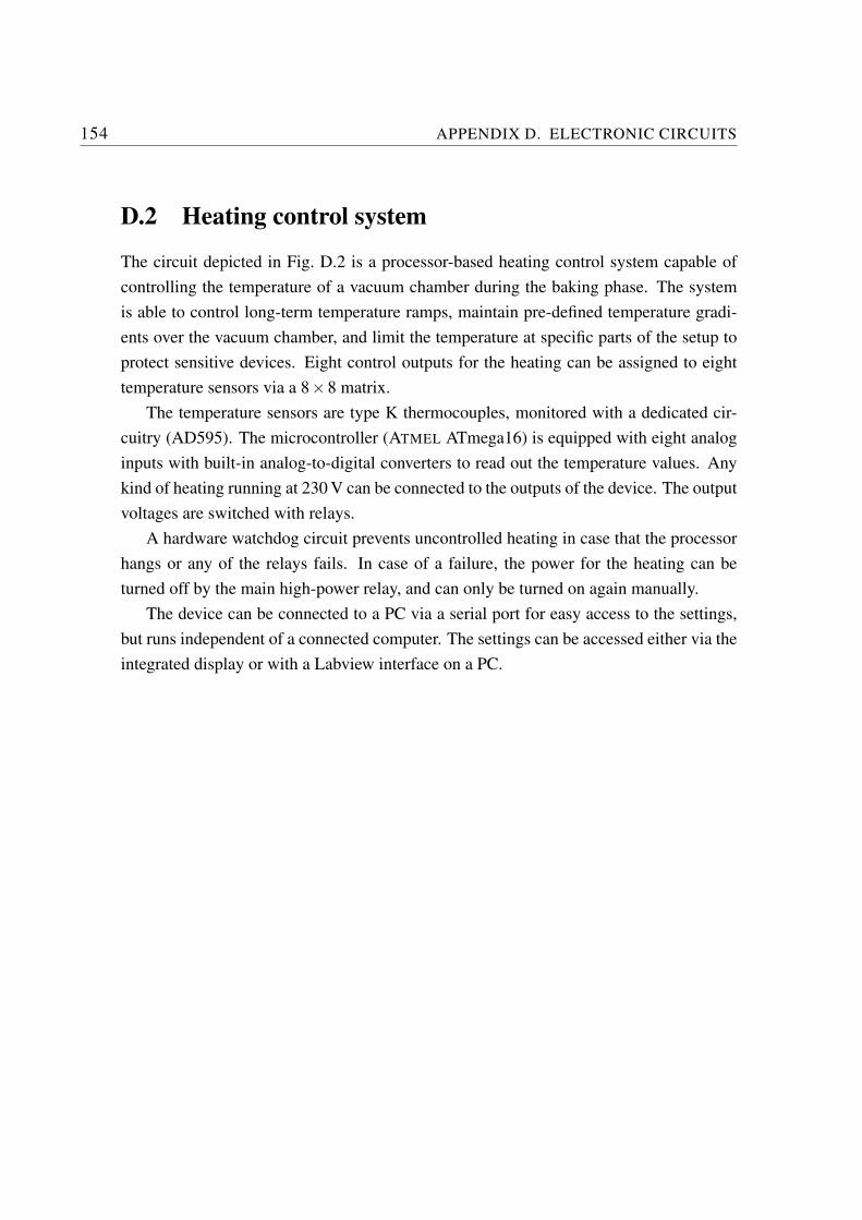
154 APPENDIX D. ELECTRONIC CIRCUITS
D.2 Heating control system
The circuit depicted in Fig. D.2 is a processor-based heating control system capable of
controlling the temperature of a vacuum chamber during the baking phase. The system
is able to control long-term temperature ramps, maintain pre-defined temperature gradi-
ents over the vacuum chamber, and limit the temperature at specific parts of the setup to
protect sensitive devices. Eight control outputs for the heating can be assigned to eight
temperature sensors via a 8×8 matrix.
The temperature sensors are type K thermocouples, monitored with a dedicated cir-
cuitry (AD595). The microcontroller (ATMEL ATmega16) is equipped with eight analog
inputs with built-in analog-to-digital converters to read out the temperature values. Any
kind of heating running at 230 V can be connected to the outputs of the device. The output
voltages are switched with relays.
A hardware watchdog circuit prevents uncontrolled heating in case that the processor
hangs or any of the relays fails. In case of a failure, the power for the heating can be
turned off by the main high-power relay, and can only be turned on again manually.
The device can be connected to a PC via a serial port for easy access to the settings,
but runs independent of a connected computer. The settings can be accessed either via the
integrated display or with a Labview interface on a PC.
D.2. HEATING CONTROL SYSTEM 155
8x
+5V
+9V
600mA
2A
display
prog
Heatin
g control
Thomas Amthor
thermocouple
LCD
8x
+ +
+
+21
Q1 C1
C2
C3
C1+
1
C1-
3
C2+
4
C2-
5
T1IN
11
T2IN
10
R1OUT
12
R2OUT
9
V+
2
V-
6
T1OUT
14
T2OUT
7
R1IN
13
R2IN
8
IC2
16
15
GND
VCC
IC2P
1 2
6 45
OK1
T1
R4
R5
21
K1
NC
NO
C
K1
D5
1 2
6 45
OK2
D6
R7
R8
C6
6
32
5
7
1
IC4
8 4
6
32
5
7
1
IC5
8 4
R9 AE
S
R10
AE
S
R11
R12
T2
C7
C8
LSP2
LSP3
C9
C10
135
24679
SV1
810
135
24679
SV2
810
(ADC7)PA7
33
(ADC6)PA6
34
(ADC5)PA5
35
(ADC4)PA4
36
(ADC3)PA3
37
(ADC2)PA2
38
(ADC1)PA1
39
(ADC0)PA0
40
(SCK)PB7
8
(MISO)PB6
7
(MOSI)PB5
6
(SS)PB4
5
(AIN1/O
C0)PB3
4
(AIN0/INT2)PB2
3
(T1)PB1
2
(T0/XCK)PB0
1
(TOSC2)PC7
29
(TOSC1)PC6
28
(TDI)PC5
27
(TDO)PC4
26
(TMS)PC3
25
(TCK)PC2
24
(SDA)PC1
23
(SCL)PC0
22
AGND
31
AVCC
30
AREF
32
XTAL1
13
XTAL2
12
VCC
10
GND
11
RESET
9
(RXD)PD0
14
(TXD)PD1
15
(INT0)PD2
16
(INT1)PD3
17
(OC1B)PD4
18
(OC1A)PD5
19
(ICP)PD6
20
(OC2)PD7
21
IC1
LSP1
R6
C11
AE
S R13
161
K3
68
4
K3
11
9
13
K3
LSP4
LSP5
LSP6
LSP7
LSP8
LSP9
T3
161
K2
11 9
13
K2
D7
LSP10
LSP11
LSP12
LSP13
-IN
14
+IN
1
+C
2
-C6
+T
3
-T5
+ALM
12
-ALM
13
FB
8
COMP
10
VO
9
V+
11
V-
7
COM
4
IC6
LSP14 LSP15
LSP16
C4
R1
LSP174MHz
33p
33p
GND
GND
VCC GND
100nGND
MAX232
CNY17
BD237
GND
1N4004
CNY17
1N4004
GND
LM311N
LM311N
GND
GND
GND
VCC VCC
GND
GND
VCC VCC
VCC
BD237
GND
GND1µ
1µ
GND
VCC
VCC
1µ
1µ
GND
ATMega16-P
GND
AGND
AGND
GND
100n
VCC
GND
+9V
GND
GND
VCC
GND
BD237
1N4004
GND
+9V
GND
AD595
VCC
AGND100n
AGND
AGND
GND
Figure D.2: Heating control system.
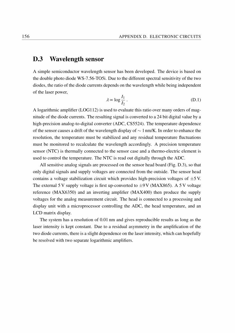
156 APPENDIX D. ELECTRONIC CIRCUITS
D.3 Wavelength sensor
A simple semiconductor wavelength sensor has been developed. The device is based on
the double photo diode WS-7.56-TO5i. Due to the different spectral sensitivity of the two
diodes, the ratio of the diode currents depends on the wavelength while being independent
of the laser power,
λ ∝ logI1
I2. (D.1)
A logarithmic amplifier (LOG112) is used to evaluate this ratio over many orders of mag-
nitude of the diode currents. The resulting signal is converted to a 24 bit digital value by a
high-precision analog-to-digital converter (ADC, CS5524). The temperature dependence
of the sensor causes a drift of the wavelength display of ∼ 1nm/K. In order to enhance the
resolution, the temperature must be stabilized and any residual temperature fluctuations
must be monitored to recalculate the wavelength accordingly. A precision temperature
sensor (NTC) is thermally connected to the sensor case and a thermo-electric element is
used to control the temperature. The NTC is read out digitally through the ADC.
All sensitive analog signals are processed on the sensor head board (Fig. D.3), so that
only digital signals and supply voltages are connected from the outside. The sensor head
contains a voltage stabilization circuit which provides high-precision voltages of ±5 V.
The external 5 V supply voltage is first up-converted to ±9V (MAX865). A 5 V voltage
reference (MAX6350) and an inverting amplifier (MAX400) then produce the supply
voltages for the analog measurement circuit. The head is connected to a processing and
display unit with a microprocessor controlling the ADC, the head temperature, and an
LCD matrix display.
The system has a resolution of 0.01 nm and gives reproducible results as long as the
laser intensity is kept constant. Due to a residual asymmetry in the amplification of the
two diode currents, there is a slight dependence on the laser intensity, which can hopefully
be resolved with two separate logarithmic amplifiers.
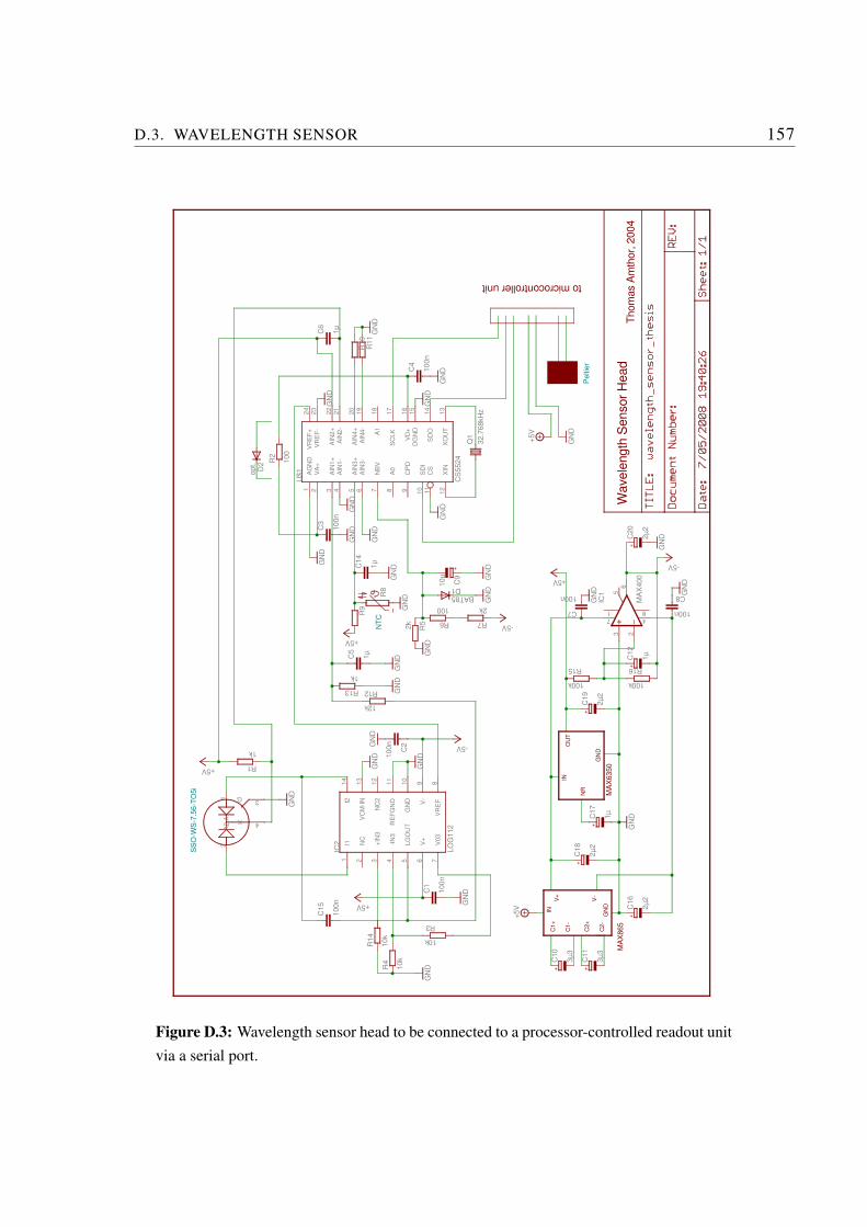
D.3. WAVELENGTH SENSOR 157
MAX865
MAX6350
C1+
C1-
C2+
C2-
GND
GND
NR
IN
V+
V-
OUT
IN
Wavelength Sensor Head
Thomas Amthor, 2004
to microcontroller unit
+
+ +
+
+
+
+
+
+
I11
NC
2
+IN3
3
-IN3
4
LGOUT
5
V+
6
V03
7VREF
8
V-
9
GND
10
REFGND
11
NC2
12
VCM-IN
13
I214
IC2
A1
1A2
2
K4
G3
Q1
C1
C2
C3
C4
C5
C6
C7
C8
R1
R2
R3
R4
R5 R6 R7
D1
C9
C10
C11
R8
AGND
1
VA+
2
AIN3+
5
AIN3-
6
NBV
7
A0
8
CPD
9
SDI
10
CS
11
XIN
12
XOUT
13
SDO
14
DGND
15
VD+
16
SCLK
17
A1
18
AIN4-
19
AIN4+
20
VREF-
23
VREF+
24
U$1 AIN1+
3
AIN1-
4AIN2+
22
AIN2-
21
R9
R10
R11
C14
D2
R12R13
R14
C15
51
236
8
IC1
7 4
C16
C17
C18
C19
C20
C12
R15 R16
LOG112
GND
GND
GND
GND
GND
GND
GND
GND
+5V
+5V
+5V
-5V
-5V
-5V
32.768kH
z
100n
100n
100n
100n
1µ
1µ
100n
100n
1k
100
10k
10k
GND
GND
GND
GNDGND
GND
GND
GND
2k
100 2k
BAT85
10µ
GND
3µ3
3µ3
CS5524
GND
GND
+5V
GND
1µ
GND
opt.
12k
1k
GND
10k
GND
100n
MAX400
GND
+5V
+5V 2µ2
1µ
2µ2
2µ2
2µ2
1µ
100k 100k
GND
GND
GND
Peltier
NTC
SSO-W
S-7.56-TO5i
Figure D.3: Wavelength sensor head to be connected to a processor-controlled readout unit
via a serial port.

158 APPENDIX D. ELECTRONIC CIRCUITS
Acknowledgements
This project was supported in part by the Landesstiftung Baden-Wurttemberg
and by the bilateral PROBRAL program of DAAD and CAPES, and it is
currently being supported by a grant of the Deutsche Forschungsgemeinschaft.
Mein besonderer Dank gilt meinem Betreuer Prof. Dr. Matthias Weidemuller, der
mir neben der Arbeit in einem spannenden Themenbereich auch viele Einblicke in die in-
ternationale Forschungswelt ermoglichte. Du hast es geschafft, mich immer zu motivieren
und zu inspirieren und hast mir zudem von Anfang an großes Vertrauen entgegengebracht.
Auch fur deine jederzeit offene Tur, viele weitblickende Ratschlage und deine immer vor-
handene Unterstutzung mochte ich mich bedanken.
Ich bin sehr dankbar fur die langjahrige Zusammenarbeit mit Markus Reetz-Lamour.
Dein Organisationstalent, deinen physikalischen Uberblick und Blick fur’s Wesentliche
habe ich immer sehr bewundert. Du hattest fur alle ein offenes Ohr und warst immer mit
einer guten Idee zur Stelle. Dies und dein besonderer Humor (und naturlich dein Sofa)
haben viel zur lockeren und motivierenden Rydberg-Atmosphare beigetragen.
Ein weiteres Dankeschon gebuhrt Kilian Singer. Menschen mit einem solchen phy-
sikalischen Verstandnis, solcher Offenheit und Herzlichkeit, wie du sie besitzt, gibt es
wirklich selten. Ich habe von unserer gemeinsamen Zeit sehr profitiert. Und durch deine
vielen unerwarteten Ideen zu ebensolchen Zeitpunkten konnte es mit dir auch nie lang-
weilig werden.
Vielen Dank an Christian Giese, der sich erfolgreich in das lange gewachsene geord-
nete Chaos im Rydberg-Labor eingearbeitet hat und einiges Know-how von ,,nebenan“
mitbrachte. Ich danke dir fur die ausgezeichnete Zusammenarbeit, deinen Humor, und
dafur, daß du auch in in stressigen Phasen die Ruhe bewahrst.
159
160 ACKNOWLEDGEMENTS
Der Erfolg des Rydberg-Projekts ist insbesondere auch der Verdienst all der großarti-
gen Diplomandinnen und Diplomanden, die am Experiment beteiligt waren oder sind. Ich
danke Johannes Deiglmayr fur viele technische Errungenschaften und die weitere ange-
nehme Gesellschaft im Nachbarlabor, Sebastian Westermann fur exzellente Berechnun-
gen und die lustige Zeit neben der Physik, Janne Denskat fur das Durchhaltevermogen
im Ringen mit russischer Fachliteratur, Christoph Hofmann fur die hervorragende Zu-
sammenarbeit und die fur die Entscheidung, den Rydbergs treu zu bleiben, Wendelin
Sprenger fur sichtbare Beats im Labor und horbare außerhalb und Hanna Schempp fur
den sehr erfolgreichen Start und wunderbare Musik.
Many international guests joined the Rydberg project for some period of time during
the past years and contributed a lot to both the scientific advances and the open and inspir-
ing working atmosphere in the group. It was a pleasure to work with Luis G. Marcassa,
Andre de Oliveira, Robin Zheng, Aigars Ekers, Nikolay Bezuglov, and Sebastian
Saliba.
Auch den Mitgliedern der anderen Projekte danke ich fur eine außerst angenehme Ar-
beitsatmosphare. Von Beginn an habe ich mich in der (damals noch kleinen) Gruppe sehr
wohlgefuhlt; dafur vielen Dank an die ,,Heidelberger“ Jorg Lange, StephanKraft, Wen-
zel Salzmann, Jochen Mikosch und Roland Wester. Das derzeitige Team besteht aus
einer Menge weiterer ganz besonderer Menschen, denen ich gleichermaßen dankbar bin,
namlich Sebastian Trippel, Rico Otto, Petr Hlavenka, Martin Stei, Anna Grochola,
Marc Repp, Karin Mortlbauer, Christian Greve, Terry Mullins, Simone Gotz, Ina
Blank und Katja Reiser. Ebenfalls vielen Dank an die ehemaligen Mitglieder unserer
Arbeitsgruppe, und das sind bereits ganz schon viele: Peter Staanum und Magnus Al-
bert (tak for gæstfriheden), Ruth Billen und Sebastian Kaiser (ohne euch ware ich wohl
nie in den Europapark gekommen), Raphael Berhane, Gerald Bock, Markus Debatin,
Christoph Eichhorn, Judith Eng, Ulrike Fruhling, Christian Gluck, Tobias Knopf,
Stefan Kohnert, Torsten Losekamm, Benjamin Muller, Ulrich Poschinger, Helmut
Rathgen, Benjamin Scherer und Leif Vogel.
I am grateful to have met and worked with all the guests and visitors of our group:
Gustavo Telles, Andrea Fioretti, Simon Bernon, Jurgen Eurisch, Andreas Stute,
Christoph Strauß, Alexander Ortner, Sagar Bora, Nathan Morrison, Mackenzie
Barton-Rowledge, and Chris Limbach.
ACKNOWLEDGEMENTS 161
Quero agradecer ao Professor Vanderlei Bagnato por ter possibilitado minha estada
em Sao Carlos, a Jorge Amin Seman e Maikel Jacob pela hospitalidade e pelos dias
inesquecıveis que passamos juntos, a Emanuel Henn pela boa cooperacao no laboratorio,
e a todos os outros membros do Grupo de Optica. Todos voces fizeram minha estada no
Brasil muito agradavel.
Außerdem danke ich Marcel Mudrich fur die Laserbau-Kooperation und naturlich
Juli fur Kuchen in der Not.
Ein ganz besonderer Dank geht an HelgaMuller, ohne deren geduldige Unterstutzung
all die Bestellungen, Reisen und Formalitaten nicht zu bewaltigen gewesen waren.
Uli Person hat uns mit einer Menge Konstruktionsarbeit beim Aufbau des Labors
sehr unterstutzt. Vielen Dank auch an Herrn Gotz fur die Wartung unserer Computer und
Drucker.
Ein großer Dank gilt den Mitarbeitern unserer großartigen Werkstatten, die alle un-
sere Ideen in reale Objekte verwandelt haben. Stellvertretend mochte ich den Leitern der
mechanischen Werkstatt, Herrn Stoll und Herrn Großmann, danken, sowie den Leitern
der Elektronikwerkstatt, Herrn Bergmann und Herrn Keilhauer, und Herrn Meyer fur
die schnelle Hilfe bei fehlenden Teilen.
Die stetige Unterstutzung und das Verstandnis meiner Eltern haben einen wichtigen
Teil zum Gelingen dieser Arbeit beigetragen und waren mir immer eine große Hilfe. Diese
Arbeit ist meinem Vater in dankbarer Erinnerung gewidmet.

162 ACKNOWLEDGEMENTS
Bibliography
[Akulin et al., 1999] Akulin, V., de Tomasi, F., Mourachko, I., and Pillet, P. (1999).
Level-band problem and many-body effects in cold Rydberg atoms. Physica D,
131:125.
[Amthor et al., 2008a] Amthor, T., Denskat, J., Giese, C., Bezuglov, N. N., Ekers, A.,
Cederbaum, L., and Weidemuller, M. (2008a). Autoionization of an ultracold Rydberg
gas through resonant dipole coupling. in prep.
[Amthor et al., 2008b] Amthor, T. et al. (2008b). Controlling the pair distribution in an
ultracold Rydberg gas. in prep.
[Amthor et al., 2008c] Amthor, T. et al. (2008c). Probing Rabi oscillations using Ramsey
interference in a three-level system. in prep.
[Amthor et al., 2007a] Amthor, T., Reetz-Lamour, M., Giese, C., and Weidemuller, M.
(2007a). Modeling many-particle mechanical effects of an interacting Rydberg gas.
Phys. Rev. A, 76:054702.
[Amthor et al., 2008d] Amthor, T., Reetz-Lamour, M., and Weidemuller, M. (2008d).
Frozen Rydberg gases. submitted.
[Amthor et al., 2007b] Amthor, T., Reetz-Lamour, M., Westermann, S., Denskat, J., and
Weidemuller, M. (2007b). Mechanical effect of van der Waals interactions observed
in real time in an ultracold Rydberg gas. Phys. Rev. Lett., 98:023004.
[Anderson et al., 2002] Anderson, W. R., Robinson, M. P., Martin, J. D. D., and Gal-
lagher, T. F. (2002). Dephasing of resonant energy transfer in a cold Rydberg gas.
Phys. Rev. A, 65:063404.
163
164 BIBLIOGRAPHY
[Anderson et al., 1998] Anderson, W. R., Veale, J. R., and Gallagher, T. F. (1998). Res-
onant dipole-dipole energy transfer in a nearly frozen Rydberg gas. Phys. Rev. Lett.,
80:249.
[Ates et al., 2008] Ates, C., Eisfeld, A., and Rost, J. M. (2008). Motion of Rydberg atoms
induced by resonant dipole-dipole interactions. New J. Phys., 10:045030.
[Atkins, 1998] Atkins, P. W. (1998). Physical Chemistry. Oxford University Press, Ox-
ford.
[Autler and Townes, 1955] Autler, S. H. and Townes, C. H. (1955). Stark effect in rapidly
varying fields. Phys. Rev., 100:703.
[Aymar, 1978] Aymar, M. (1978). Influence of core-polarisation effects on the photoion-
isation cross sections of the ground level and excited ns levels of neutral sodium. J.
Phys. B, 11:1413.
[Balmer, 1885] Balmer, J. J. (1885). Notiz uber die Spectrallinien des Wasserstoffs. Ann.
Phys. Chem., 25:80.
[Berman and Salomaa, 1982] Berman, P. R. and Salomaa, R. (1982). Comparison be-
tween dressed-atom and bare-atom pictures in laser spectroscopy. Phys. Rev. A,
25:2667.
[Beterov et al., 2007] Beterov, I. I., Tretyakov, D. B., Ryabtsev, I. I., Ekers, A., and Bezu-
glov, N. N. (2007). Ionization of sodium and rubidium ns, np, and nd Rydberg atoms
by blackbody radiation. Phys. Rev. A, 75:052720.
[Bhatti et al., 1981] Bhatti, S. A., Cromer, C. L., and Cooke, W. E. (1981). Analysis of
the Rydberg character of the 5d7d1d2 state of barium. Phys. Rev. A, 24:161.
[Birkl et al., 2001] Birkl, G., Buchkremer, F. B. J., Dumke, R., and Ertmer, W. (2001).
Atom optics with microfabricated optical elements. Opt. Comm., 191:67.
[Birkl and Fortagh, 2007] Birkl, G. and Fortagh, J. (2007). Micro traps for quantum in-
formation processing and presicion force sensing. Laser & Photon. Rev., 1:12.
[Bjorklund, 1980] Bjorklund, G. C. (1980). Frequency-modulation spectroscopy: a new
method for measuring weak absorptions and dispersions. Opt. Lett., 5:15.
BIBLIOGRAPHY 165
[Blatt, 1967] Blatt, J. M. (1967). Practical points concerning the solution of the
Schrodinger equation. J. Comput. Phys., 1:382.
[Bohr, 1913] Bohr, N. (1913). On the constitution of atoms and molecules. Phil. Mag.,
26:1.
[Boisseau et al., 2002] Boisseau, C., Simbotin, I., and Cote, R. (2002). Macrodimers:
Ultralong range Rydberg molecules. Phys. Rev. Lett., 88:133004.
[Brion et al., 2007a] Brion, E., Mølmer, K., and Saffman, M. (2007a). Quantum comput-
ing with collective ensembles of multilevel systems. Phys. Rev. Lett., 99:260501.
[Brion et al., 2007b] Brion, E., Pedersen, L. H., and Mølmer, K. (2007b). Implementing
a neutral atom Rydberg gate without populating the Rydberg state. J. Phys. B, 40:S159.
[Bronstein et al., 2000] Bronstein, I. N., Semendjajew, K. A., Musiol, G., and Muhlig, H.
(2000). Taschenbuch der Mathematik. Harri Deutsch, Frankfurt.
[Cheret and Barbier, 1984] Cheret, M. and Barbier, L. (1984). Experimental evidence
for negative-ion formation by the collisional reaction Rb(6d)+Rb(5s) →Rb++Rb−.
Phys. Rev. A, 30:1132.
[Chibisov, 2007] Chibisov, M. I. (2007). Coulomb Rydberg electron l-mixing in colli-
sions with atomic ions. J. Exp. Theor. Phys., 105:926.
[Chibisov et al., 2002] Chibisov, M. I., Khuskivadze, A. A., and Fabrikant, I. I. (2002).
Energies and dipole moments of long-range molecular Rydberg states. J. Phys. B,
35:L193.
[Ciocca et al., 1986] Ciocca, M., Allegrini, M., Arimondo, E., Burkhardt, C. E., Garver,
W. P., and Leventhal, J. J. (1986). Negative ion formation in Rydberg-atom interactions
(n = 7−40). Phys. Rev. Lett., 56:704.
[Cogdell et al., 2006] Cogdell, R. J., Gall, A., and Kohler, J. (2006). The architecture and
function of the light-harvesting apparatus of purple bacteria: from single molecules to
in vivo membranes. Quarterly Review of Biophysics, 39:227.
[Cohen-Tannoudji et al., 1999] Cohen-Tannoudji, C., Diu, B., and Laloe, F. (1999).
Quantenmechanik. W. de Gruyter, Berlin.
166 BIBLIOGRAPHY
[Cohen-Tannoudji et al., 1998] Cohen-Tannoudji, C., Dupont-Roc, J., and Grynberg, G.
(1998). Atom–Photon Interactions. John Wiley & Sons, New York.
[Cozzini et al., 2006] Cozzini, M., Calarco, T., Recati, A., and Zoller, P. (2006). Fast
Rydberg gates without dipole blockade via quantum control. Opt. Comm., 264:375.
[Cubel et al., 2005] Cubel, T., Teo, B. K., Malinovsky, V. S., Guest, J. R., Reinhard, A.,
Knuffman, B., Berman, P. R., and Raithel, G. (2005). Coherent population transfer of
ground-state atoms into Rydberg states. Phys. Rev. A, 72:023405.
[Cubel Liebisch et al., 2005] Cubel Liebisch, T., Reinhard, A., Berman, P. R., and
Raithel, G. (2005). Atom counting statistics in ensembles of interacting Rydberg
atoms. Phys. Rev. Lett., 95:253002.
[Cummings et al., 2005] Cummings, E. A., Daily, J. E., Durfee, D. S., and Bergeson,
S. D. (2005). Fluorescence measurements of expanding strongly coupled neutral plas-
mas. Phys. Rev. Lett., 95:235001.
[Day et al., 2008] Day, J. O., Brekke, E., and Walker, T. G. (2008). Dynamics of low-
density ultracold Rydberg gases. Phys. Rev. A, 77:052712.
[de Oliveira et al., 2002] de Oliveira, A. L., Mancini, M. W., Bagnato, V. S., and Mar-
cassa, L. G. (2002). Measurement of Rydberg-state lifetimes using cold trapped atoms.
Phys. Rev. A, 65:031401.
[Deiglmayr, 2006] Deiglmayr, J. (2006). Coherent excitation of an ultracold gas of Ryd-
berg atoms. Diploma thesis, Physikalisches Institut, Universitat Freiburg.
[Deiglmayr et al., 2006] Deiglmayr, J., Reetz-Lamour, M., Amthor, T., Westermann, S.,
de Oliveira, A. L., and Weidemuller, M. (2006). Coherent excitation of Rydberg atoms
in an ultracold gas. Opt. Comm., 264:293.
[Devoret et al., 1992] Devoret, M. H., Esteve, D., and Urbina, C. (1992). Single-electron
transfer in metallic nanostructures. Nature, 360:547.
[Ducas et al., 1975] Ducas, T. W., Littman, M. G., Freeman, R. R., and Kleppner, D.
(1975). Stark ionization of high-lying states of sodium. Phys. Rev. Lett., 35:366.
BIBLIOGRAPHY 167
[Dutta et al., 2001] Dutta, S. K., Feldbaum, D., Walz-Flannigan, A., Guest, J. R., and
Raithel, G. (2001). High-angular-momentum states in cold Rydberg gases. Phys. Rev.
Lett., 86:3993.
[Engel et al., 2007] Engel, G. S., Calhoun, T. R., Read, E. L., Ahn, T.-K., Mancal, T.,
Cheng, Y.-C., Blankenship, R. E., and Fleming, G. R. (2007). Evidence for wave-
like energy transfer through quantum coherence in photosynthetic systems. Nature,
446:782.
[Farooqi et al., 2003] Farooqi, S. M., Tong, D., Krishnan, S., Stanojevic, J., Zhang, Y. P.,
Ensher, J. R., Estrin, A. S., Boisseau, C., Cote, R., Eyler, E. E., and Gould, P. L. (2003).
Long-range molecular resonances in a cold Rydberg gas. Phys. Rev. Lett., 91:183002.
[Folling, 2003] Folling, S. (2003). 3d Raman sideband cooling of rubidium – towards an
ultracold, dense ensemble of Rydberg atoms. Diploma thesis, Max-Planck-Institut fur
Kernphysik, Heidelberg, Universitat Heidelberg.
[Forster, 1948] Forster, T. (1948). Zwischenmolekulare Energieumwandlung und Fluo-
reszenz. Ann. Phys., 437:55.
[Fortagh et al., 1998] Fortagh, J., Grossmann, A., Hansch, T. W., and Zimmermann, C.
(1998). Fast loading of a magneto-optical trap from a pulsed thermal source. J. Appl.
Phys., 84:6499.
[Fuso et al., 1992] Fuso, F., Allegrini, M., Arimondo, E., and Manson, S. T. (1992).
Model for atomic multiphoton ionization via Rydberg states. Z. Phys. D, 23:233.
[Galitskii et al., 1981] Galitskii, V. M., Nikitin, E. E., and Smirnov, B. M., editors (1981).
Theory of the Collisions of Atomic Particles (in Russian). Nauka, Moscow.
[Gallagher and Pritchard, 1989] Gallagher, A. and Pritchard, D. E. (1989). Exoergic col-
lisions of cold Na*-Na. Phys. Rev. Lett., 63:957.
[Gallagher, 1994] Gallagher, T. F. (1994). Rydberg Atoms. Cambridge University Press,
Cambridge.
[Gallagher et al., 1976] Gallagher, T. F., Humphrey, T. M., Hill, R. M., and Edelstein,
S. A. (1976). Resolution of |ml| and |m j| levels in the electric field ionization of highly
excited d states of Na. Phys. Rev. Lett., 37:1465.
168 BIBLIOGRAPHY
[Gallagher et al., 2003] Gallagher, T. F., Pillet, P., Robinson, M. P., Laburthe-Tolra, B.,
and Noel, M. W. (2003). Back and forth between Rydberg atoms and ultracold plasmas.
J. Opt. Soc. Am. B, 20:1091.
[Gounand et al., 1979] Gounand, F., Hugon, M., Fournier, P. R., and Berlande, J. (1979).
Superradiant cascading effects in rubidium Rydberg levels. J. Phys. B, 12:547.
[Granger et al., 2001] Granger, B. E., Hamilton, E. L., and Greene, C. H. (2001). Quan-
tum and semiclassical analysis of long-range Rydberg molecules. Phys. Rev. A,
64:042508.
[Greene et al., 2000] Greene, C. H., Dickinson, A. S., and Sadeghpour, H. R. (2000).
Creation of polar and nonpolar ultra-long-range Rydberg molecules. Phys. Rev. Lett.,
85:2458.
[Greene et al., 2006] Greene, C. H., Hamilton, E. L., Crowell, H., Vadla, C., and Niemax,
K. (2006). Experimental verification of minima in excited long-range Rydberg states
of Rb2. Phys. Rev. Lett., 97:233002.
[Gregg, 2003] Gregg, B. A. (2003). Excitonic solar cells. J. Phys. Chem. B, 107:4688.
[Grimm et al., 1999] Grimm, R., Weidemuller, M., and Ovchinnikov, Y. B. (1999). Op-
tical dipole traps for neutral atoms. arXiv:physics/9902072.
[Hader, 1999] Hader, D.-P., editor (1999). Photosynthese. Georg Thieme Verlag,
Stuttgart.
[Hamilton et al., 2002] Hamilton, E. L., Greene, C. H., and Sadeghpour, H. R. (2002).
Shape-resonance-induced long-range molecular Rydberg states. J. Phys. B, 35:L199.
[Han and Gallagher, 2008] Han, J. and Gallagher, T. F. (2008). Field ionization of the
frozen Rydberg gas. Phys. Rev. A, 77:015404.
[Heidemann et al., 2007] Heidemann, R., Raitzsch, U., Bendkowsky, V., Butscher, B.,
Low, R., Santos, L., and Pfau, T. (2007). Evidence for coherent collective Rydberg
excitation in the strong blockade regime. Phys. Rev. Lett., 99:163601.
[Heidemann et al., 2008] Heidemann, R., Raitzsch, U., Bendowsky, V., Butscher, B.,
Low, R., and Pfau, T. (2008). Rydberg excitation of Bose-Einstein condensates. Phys.
Rev. Lett., 100:033601.
BIBLIOGRAPHY 169
[Henn et al., 2007] Henn, E. A. L., Seman, J. A., Ramos, E. R. F., Iavaronni, A. H.,
Amthor, T., and Bagnato, V. S. (2007). Evaporation in atomic traps: A simple ap-
proach. Am. J. Phys., 75:907.
[Hertz, 1909] Hertz, P. (1909). Uber den gegenseitigen durchschnittlichen Abstand von
Punkten, die mit bekannter mittlerer Dichte im Raume angeordnet sind. Math. Ann.,
67:387.
[Hofmann et al., 2004] Hofmann, C., Aartsma, T. J., Michel, H., and Kohler, J. (2004).
Spectral dynamics in the B800 band of LH2 from Rhodospirillum molischianum - a
single molecule study. New Journal of Physics, 6:8.
[Hofmann, 2008] Hofmann, C. S. (2008). Spectroscopy of an interacting ultracold Ryd-
berg gas. Diploma thesis, Universitat Freiburg.
[Iavaronni et al., 2007] Iavaronni, A. H., Henn, E. A. L., Ramos, E. R. F., Seman, J. A.,
Amthor, T., and Bagnato, V. S. (2007). Evaporacao em armadilhas atomicas e as
temperaturas mais baixas do universo. Rev. Bras. Ens. Fıs., 29:209.
[Jackson, 1975] Jackson, J. D. (1975). Classical Electrodynamics. John Wiley & Sons,
New York.
[Jaksch et al., 2000] Jaksch, D., Cirac, J. I., Zoller, P., Rolston, S. L., Cote, R., and Lukin,
M. D. (2000). Fast quantum gates for neutral atoms. Phys. Rev. Lett., 85:2208.
[Jares-Erijman and Jovin, 2003] Jares-Erijman, E. A. and Jovin, T. M. (2003). FRET
imaging. Nature Biotechnology, 21:1387.
[Johnson et al., 2008] Johnson, T. A., Urban, E., Henage, T., Isenhower, L., Yavuz, D. D.,
Walker, T. G., and Saffman, M. (2008). Rabi oscillations between ground and Rydberg
states with dipole-dipole atomic interactions. Phys. Rev. Lett., 100:113003.
[Kaiser et al., 1991] Kaiser, R., Vansteenkiste, N., Aspect, A., E., E. A., and Cohen-
Tannoudji, C. (1991). Mechanical Hanle effect. Z. Phys. D, 18:17.
[Khuskivadze et al., 2002] Khuskivadze, A. A., Chibisov, M. I., and Fabrikant, I. I.
(2002). Adiabatic energy levels and electric dipole moments of Rydberg states of
Rb2 and Cs2 dimers. Phys. Rev. A, 66:042709.
170 BIBLIOGRAPHY
[Killian, 2007] Killian, T. C. (2007). Ultracold neutral plasmas. Science, 316:705.
[Killian et al., 2001] Killian, T. C., Lim, M. J., Kulin, S., Dumke, R., Bergeson, S. D.,
and Rolston, S. L. (2001). Formation of Rydberg atoms in an expanding ultracold
neutral plasma. Phys. Rev. Lett., 86:3759.
[Killian et al., 2007] Killian, T. C., Pattard, T., Pohl, T., and Rost, J. M. (2007). Ultracold
neutral plasmas. Physics Reports, 449:77.
[Knuffman and Raithel, 2006] Knuffman, B. and Raithel, G. (2006). Emission of fast
atoms from a cold Rydberg gas. Phys. Rev. A, 73:020704(R).
[Kohler, 2001] Kohler, J. (2001). Photosynthese und Exzitonen. Physikalische Blatter,
56(1):47.
[Kulin et al., 2000] Kulin, S., Killian, T. C., Bergeson, S. D., and Rolston, S. L. (2000).
Plasma oscillations and expansion of an ultracold neutral plasma. Phys. Rev. Lett.,
85:318.
[Lehman, 1983] Lehman, G. W. (1983). Rate of ionisation of H and Na Rydberg atoms
by black-body radiation. J. Phys. B, 16:2145.
[Li et al., 2003] Li, W., Mourachko, I., Noel, M. W., and Gallagher, T. F. (2003).
Millimeter-wave spectroscopy of cold Rb Rydberg atoms in a magneto-optical trap:
Quantum defects of the ns, np, and nd series. Phys. Rev. A, 67:052502.
[Li et al., 2004] Li, W., Noel, M. W., Robinson, M. P., Tanner, P. J., Gallagher, T. F.,
Comparat, D., Tolra, B. L., Vanhaecke, N., Vogt, T., Zahzam, N., and Pillet, P. (2004).
Evolution dynamics of a dense frozen Rydberg gas to plasma. Phys. Rev. A, 70:042713.
[Li et al., 2005] Li, W., Tanner, P. J., and Gallagher, T. F. (2005). Dipole-dipole excitation
and ionization in an ultracold gas of Rydberg atoms. Phys. Rev. Lett., 94:173001.
[Liu and Rost, 2006] Liu, I. C. H. and Rost, J. M. (2006). Polyatomic molecules formed
with a Rydberg atom in an ultracold environment. Eur. Phys. J. D, 40:65.
[Lorenzen and Niemax, 1983] Lorenzen, C. J. and Niemax, K. (1983). Quantum defects
of the n2P1/2,3/2 levels in 39K I and 85Rb I. Physica Scripta, 27:300–305.
BIBLIOGRAPHY 171
[Lukin et al., 2001] Lukin, M. D., Fleischhauer, M., Cote, R., Duan, L. M., Jaksch, D.,
Cirac, J. I., and Zoller, P. (2001). Dipole blockade and quantum information processing
in mesoscopic atomic ensembles. Phys. Rev. Lett., 87:037901.
[Macdonald, 1992] Macdonald, J. R. (1992). Nearest-neighbor distribution functions and
mean separation for impenetrable particles in one to three dimensions. Phys. Rev. A,
46:R2988.
[Magalhaes et al., 2000] Magalhaes, K., de Oliveira, A., Zanon, R., Bagnato, V., and
Marcassa, L. (2000). Lifetime determination of high excited states of 85Rb using a
sample of cold atoms. Opt. Comm., 184:385.
[Marinescu et al., 1994] Marinescu, M., Sadeghpour, H. R., and Dalgarno, A. (1994).
Dispersion coefficients for alkali-metal dimers. Phys. Rev. A, 49:982.
[Mohapatra et al., 2008] Mohapatra, A. K., Bason, M. G., Butscher, B., Weatherill, K. J.,
and Adams, C. S. (2008). Giant electro-optic effect using polarizable dark states.
arXiv:0804.3273v1.
[Mohapatra et al., 2007] Mohapatra, A. K., Jackson, T. R., and Adams, C. S. (2007).
Coherent optical detection of highly excited Rydberg states using electromagnetically
induced transparency. Phys. Rev. Lett., 98:113003.
[Møller et al., 2008] Møller, D., Madsen, L. B., and Mølmer, K. (2008). Quantum gates
and multiparticle entanglement by Rydberg excitation blockade and adiabatic passage.
Phys. Rev. Lett., 100:170504.
[Mourachko et al., 1998] Mourachko, I., Comparat, D., de Tomasi, F., Fioretti, A., Nos-
baum, P., Akulin, V. M., and Pillet, P. (1998). Many-body effects in a frozen Rydberg
gas. Phys. Rev. Lett., 80:253.
[Mourachko et al., 2004] Mourachko, I., Li, W., and Gallagher, T. F. (2004). Controlled
many-body interactions in a frozen Rydberg gas. Phys. Rev. A, 70:031401.
[Mudrich et al., 2005] Mudrich, M., Zahzam, N., Vogt, T., Comparat, D., and Pillet, P.
(2005). Back and forth transfer and coherent coupling in a cold Rydberg dipole gas.
Phys. Rev. Lett., 95:233002.
172 BIBLIOGRAPHY
[Mulken et al., 2007] Mulken, O., Blumen, A., Amthor, T., Giese, C., Reetz-Lamour, M.,
and Weidemuller, M. (2007). Survival probabilities in coherent exciton transfer with
trapping. Phys. Rev. Lett., 99:090601.
[NIST, 2005] NIST (2005). Atomic spectra database v3.0.
http://physics.nist.gov/PhysRefData/ASD1/.
[Numerov, 1927] Numerov, B. (1927). Note on the numerical integration of d2x/dt2 =
f (x, t). Astron. Nachr., 230:359.
[Numerov, 1924] Numerov, B. V. (1924). A method of extrapolation of perturbations.
Mon. Not. R. Astron. Soc., 84:592.
[Olson, 1979] Olson, R. (1979). Ionization cross sections for Rydberg-atom–Rydberg-
atom collisions. Phys. Rev. Lett., 43:126.
[Orrit, 1999] Orrit, M. (1999). Coherent excitation in the antenna complex. Science,
285:349.
[Overstreet et al., 2007] Overstreet, K. R., Schwettmann, A., Tallant, J., and Shaffer,
J. P. (2007). Photoinitiated collisions between cold Cs Rydberg atoms. Phys. Rev.
A, 76:011403(R).
[Pohl et al., 2003] Pohl, T., Pattard, T., and Rost, J. M. (2003). Plasma formation from
ultracold Rydberg gases. Phys. Rev. A, 68:010703.
[Raab et al., 1987] Raab, E. L., Prentiss, M., Cable, A., Chu, S., and Pritchard, D. E.
(1987). Trapping of neutral sodium atoms with radiation pressure. Phys. Rev. Lett.,
59:2631.
[Raitzsch et al., 2008] Raitzsch, U., Bendkowsky, V., Heidemann, R., Butscher, B., Low,
R., and Pfau, T. (2008). Echo experiments in a strongly interacting Rydberg gas. Phys.
Rev. Lett., 100:013002.
[Reetz-Lamour, 2006] Reetz-Lamour, M. (2006). Coherence and decoherence in an ul-
tracold gas of Rydberg atoms. PhD thesis, Universitat Freiburg.
[Reetz-Lamour et al., 2008a] Reetz-Lamour, M., Amthor, T., Deiglmayr, J., and Wei-
demuller, M. (2008a). Rabi oscillations and excitation trapping in the coherent excita-
tion of a mesoscopic frozen Rydberg gas. Phys. Rev. Lett., 100:253001.
BIBLIOGRAPHY 173
[Reetz-Lamour et al., 2006] Reetz-Lamour, M., Amthor, T., Deiglmayr, J., Westermann,
S., Singer, K., de Oliveira, A. L., Marcassa, L. G., and Weidemuller, M. (2006).
Prospects of ultracold Rydberg gases for quantum information processing. Fortschr.
Phys., 54:776.
[Reetz-Lamour et al., 2007] Reetz-Lamour, M., Amthor, T., Westermann, S., Denskat, J.,
de Oliveira, A. L., and Weidemuller, M. (2007). Modeling few-body phenomena in an
ultracold Rydberg gas. Nucl. Phys. A, 790:728c.
[Reetz-Lamour et al., 2008b] Reetz-Lamour, M., Deiglmayr, J., Amthor, T., and Wei-
demuller, M. (2008b). Rabi oscillations between ground and Rydberg states and van
der Waals blockade in a mesoscopic frozen Rydberg gas. New J. Phys., 10:045026.
[Reinhard et al., 2008] Reinhard, A., Liebisch, T. C., Younge, K. C., Berman, P. R., and
Raithel, G. (2008). Rydberg-Rydberg collisions: Resonant enhancement of state mix-
ing and Penning ionization. Phys. Rev. Lett., 100:123007.
[Ricci et al., 1995] Ricci, L., Weidemuller, M., Esslinger, T., Hemmerich, A., Zimmer-
mann, C., Vuletic, V., Konig, W., and Hansch, T. W. (1995). A compact grating-
stabilized diode laser system for atomic physics. Opt. Comm., 117:541–549.
[Ritz and Schulten, 2001] Ritz, T. and Schulten, K. (2001). Physik der Photosynthese.
Physikalische Bltter, 57(2):49.
[Roberts et al., 2004] Roberts, J. L., Fertig, C. D., Lim, M. J., and Rolston, S. L. (2004).
Electron temperature of ultracold plasmas. Phys. Rev. Lett., 92:253003.
[Robicheaux, 2005] Robicheaux, F. (2005). Ionization due to the interaction between
two Rydberg atoms. J. Phys. B, 38:S333.
[Robicheaux and Hanson, 2002] Robicheaux, F. and Hanson, J. D. (2002). Simulation of
the expansion of an ultracold neutral plasma. Phys. Rev. Lett., 88:055002.
[Robinson et al., 2000] Robinson, M. P., Tolra, B. L., Noel, M. W., Gallagher, T. F., and
Pillet, P. (2000). Spontaneous evolution of Rydberg atoms into an ultracold plasma.
Phys. Rev. Lett., 85:4466.
174 BIBLIOGRAPHY
[Ryabtsev et al., 2005] Ryabtsev, I. I., Tretyakov, D. B., Beterov, I. I., Bezuglov, N. N.,
Miculis, K., and Ekers, A. (2005). Collisional and thermal ionization of sodium Ryd-
berg atoms: I. Experiment for nS and nD atoms with n = 8−20. J. Phys. B, 38:S17.
[Saffman and Mølmer, 2008] Saffman, M. and Mølmer, K. (2008). Scaling the neu-
tral atom Rydberg gate quantum computer by collective encoding in holmium atoms.
arXiv:0805.0440v1.
[Sakurai, 1994] Sakurai, J. J. (1994). Modern Quantum Mechanics. Addison Wesley,
Reading, Massachusetts.
[Schlosser and Lochbrunner, 2006] Schlosser, M. and Lochbrunner, S. (2006). Exciton
migration by ultrafast Forster transfer in highly doped matrixes. J. Phys. Chem. B,
110:6001.
[Schwettmann et al., 2006] Schwettmann, A., Crawford, J., Overstreet, K. R., and Shaf-
fer, J. P. (2006). Cold Cs Rydberg-gas interactions. Phys. Rev. A, 74:020701(R).
[Shiozaki et al., 2007] Shiozaki, R. F., Henn, E. A. L., Magalhaes, K. M. F., Amthor, T.,
and Bagnato, V. S. (2007). Tunable eletro-optical modulators based on a split-ring
resonator. Rev. Sci. Inst., 78:016103.
[Shirley, 1982] Shirley, J. H. (1982). Modulation transfer processes in optical heterodyne
saturation spectroscopy. Opt. Lett., 7:537.
[Simien et al., 2004] Simien, C. E., Chen, Y. C., Gupta, P., Laha, S., Martinez, Y. N.,
Mickelson, P. G., Nagel, S. B., and Killian, T. C. (2004). Using absorption imaging to
study ion dynamics in an ultracold neutral plasma. Phys. Rev. Lett., 92:143001.
[Singer et al., 2005a] Singer, K., Reetz-Lamour, M., Amthor, T., Folling, S., Tscherneck,
M., and Weidemuller, M. (2005a). Spectroscopy of an ultracold Rydberg gas and
signatures of Rydberg–Rydberg interactions. J. Phys. B, 38:S321.
[Singer et al., 2004] Singer, K., Reetz-Lamour, M., Amthor, T., Marcassa, L. G., and
Weidemuller, M. (2004). Suppression of excitation and spectral broadening induced
by interactions in a cold gas of Rydberg atoms. Phys. Rev. Lett., 93:163001.
BIBLIOGRAPHY 175
[Singer et al., 2005b] Singer, K., Stanojevic, J., Weidemuller, M., and Cote, R. (2005b).
Long-range interactions between alkali Rydberg atom pairs correlated to the ns-ns,
np-np and nd-nd asymptotes. J. Phys. B, 38:S295.
[Spencer et al., 1982a] Spencer, W. P., Vaidyanathan, A. G., Kleppner, D., and Ducas,
T. W. (1982a). Photoionization by blackbody radiation. Phys. Rev. A, 26:1490.
[Spencer et al., 1982b] Spencer, W. P., Vaidyanathan, A. G., Kleppner, D., and Ducas,
T. W. (1982b). Temperature dependence of blackbody-radiation-induced transfer
among highly excited states of sodium. Phys. Rev. A, 25:380.
[Stanojevic et al., 2006] Stanojevic, J., Cote, R., Tong, D., Farooqi, S. M., Eyler, E. E.,
and Gould, P. L. (2006). Long-range Rydberg–Rydberg interactions and molecular
resonances. Eur. Phys. J. D, 40:3.
[Stebbings et al., 1975] Stebbings, R. F., Latimer, C. J., West, W. P., Dunning, F. B., and
Cook, T. B. (1975). Studies of xenon atoms in high Rydberg states. Phys. Rev. A,
12:1453.
[Steck, 2002] Steck, D. A. (2002). Rubidium 87 d line data.
[Stoneman et al., 1987] Stoneman, R. C., Adams, M. D., and Gallagher, T. F. (1987).
Resonant-collision spectroscopy of Rydberg atoms. Phys. Rev. Lett., 58:1324.
[Tanner et al., 2008] Tanner, P. J., Han, J., Shuman, E. S., and Gallagher, T. F. (2008).
Many-body ionization in a frozen Rydberg gas. Phys. Rev. Lett., 100:043002.
[Theodosiou and Fielder Jr., 1982] Theodosiou, C. E. and Fielder Jr., W. (1982). Pho-
toionisation of the outermost closed shell of the alkali metal atoms. J. Phys. B, 15:4113.
[Tong et al., 2004] Tong, D., Farooqi, S. M., Stanojevic, J., Krishnan, S., Zhang, Y. P.,
Cote, R., Eyler, E. E., and Gould, P. L. (2004). Local blockade of Rydberg excitation
in an ultracold gas. Phys. Rev. Lett., 93:063001.
[Torquato et al., 1990] Torquato, S., Lu, B., and Rubinstein, J. (1990). Nearest-neighbor
distribution functions in many-body systems. Phys. Rev. A, 41:2059.
[Tscherneck, 2002] Tscherneck, M. (2002). Aufbau eines Experimentes zur Erzeugung
ultrakalter, dichter Gase unter Verwendung eines neuartigen Lasersystems. Diploma
thesis, Max-Planck-Institut fur Kernphysik, Heidelberg, Universitat Heidelberg.
176 BIBLIOGRAPHY
[Urban et al., 2008] Urban, E., Johnson, T. A., Henage, T., Isenhower, L., Yavuz, D. D.,
Walker, T. G., , and Saffman, M. (2008). Observation of Rydberg blockade between
two atoms. arXiv:0805.0758v1.
[Vitrant et al., 1982] Vitrant, G., Raimond, J. M., Gross, M., and Haroche, S. (1982).
Rydberg to plasma evolution in a dense gas of very excited atoms. J. Phys. B, 15:L49.
[Vogt et al., 2007] Vogt, T., Viteau, M., Chotia, A., Zhao, J., Comparat, D., and Pillet, P.
(2007). Electric-field induced dipole blockade with Rydberg atoms. Phys. Rev. Lett.,
99:073002.
[Vogt et al., 2006] Vogt, T., Viteau, M., Zhao, J., Chotia, A., Comparat, D., and Pillet,
P. (2006). Dipole blockade at forster resonances in high resolution laser excitation of
Rydberg states of cesium atoms. Phys. Rev. Lett., 97:083003.
[Walz-Flannigan et al., 2004] Walz-Flannigan, A., Guest, J. R., Choi, J.-H., and Raithel,
G. (2004). Cold-Rydberg-gas dynamics. Phys. Rev. A, 69:063405.
[Wang et al., 2007] Wang, T., Yelin, S. F., Cote, R., Eyler, E. E., Farooqi, S. M., Gould,
P. L., Kostrun, M., Tong, D., and Vrinceanu, D. (2007). Superradiance in ultracold
Rydberg gases. Phys. Rev. A, 75:033802.
[Weidemuller and Grimm, 1999] Weidemuller, M. and Grimm, R. (1999). Optische
Dipolfallen: Experimente mit ultrakalten Atomen und anderen kleinen Teilchen im
Lichtkafig. Physikalische Blatter, 55:41.
[Weidemuller et al., 2005] Weidemuller, M., Reetz-Lamour, M., Amthor, T., Deiglmayr,
J., and Singer, K. (2005). Interactions in an ultracold gas of Rydberg atoms. Laser
Spectroscopy XVII (ICOLS Proceedings), page 264.
[Weidemuller et al., 2004] Weidemuller, M., Singer, K., Reetz-Lamour, M., Amthor, T.,
and Marcassa, L. G. (2004). Ultralong-range interactions and blockade of excitation
in a cold Rydberg gas. Atomic Physics XIX (ICAP Proceedings), page 157.
[Weimer et al., 2008] Weimer, H., Low, R., Pfau, T., and Buchler, H. P. (2008). Quantum
critical behavior in strongly interacting Rydberg gases. arXiv:0806.3754.
BIBLIOGRAPHY 177
[West et al., 1976] West, W. P., Foltz, G. W., Dunning, F. B., Latimer, C. J., and Steb-
bings, R. F. (1976). Absolute measurements of collisional ionization of xenon atoms
in well-defined high Rydberg states. Phys. Rev. Lett., 36:854.
[Westermann, 2006] Westermann, S. (2006). Resonant energy transfer in ultracold Ryd-
berg gases. Diploma thesis, Universitat Freiburg.
[Westermann et al., 2006] Westermann, S., Amthor, T., de Oliveira, A. L., Deiglmayr, J.,
Reetz-Lamour, M., and Weidemuller, M. (2006). Dynamics of resonant energy transfer
in a cold Rydberg gas. Eur. Phys. J. D, 40:37.
[Whitley and Stroud, Jr., 1976] Whitley, R. M. and Stroud, Jr., C. R. (1976). Double
optical resonance. Phys. Rev. A, 14:1498.
[Wilkinson et al., 1996] Wilkinson, S. R., Smith, A. V., Scully, M. O., and Fry, E. (1996).
Observation of interference fringes in Autler-Townes line shapes. Phys. Rev. A, 53:126.
[Wright et al., 2005] Wright, M., Gensemer, S., Vala, J., Kosloff, R., and Gould, P.
(2005). Control of ultracold collisions with frequency-chirped light. Phys. Rev. Lett.,
95:063001.
[Wright et al., 2007] Wright, M. J., Pechkis, J. A., Carini, J. L., Kallush, S., Kosloff, R.,
and Gould, P. L. (2007). Coherent control of ultracold collisions with chirped light:
Direction matters. Phys. Rev. A, 75:051401.
[Zimmerman et al., 1979] Zimmerman, M. L., Littman, M. G., Kash, M. M., and Klepp-
ner, D. (1979). Stark structure of the Rydberg states of alkali-metal atoms. Phys. Rev.
A, 20:2251.