Interaction Effects in Econometrics

October 16, 2011

Abstract

We provide practical advice for applied economists regarding robust specificationand interpretation of linear regression models with interaction terms. We replicatea number of prominent published results using interaction effects and examine ifthey are robust to reasonable specification permutations.

JEL classification: C12, C13Keywords: Non-Linear Regression, Interaction Terms.

1 Introduction

A country may consider a reform that would strengthen the financial sector. Would

this help economic growth and development? This simple question is frustratingly hard

to answer using empirical data because economic development itself spawns financial

development, so while economic and financial developments are positively correlated

this does not answer the question asked. In a highly influential paper, Rajan and

Zingales (1998) provide convincing evidence that financial development is important for

economic development by asking the simple question: do industrial sectors that are more

dependent on external finance grow faster in countries with a high level of development.

This question involves interactions between financial development and dependency on

external finance. Since the publication of Rajan and Zingales’ highly influential study,

the estimation of models with interaction effects have become very common in applied

economics.

Many articles applying interaction terms are motivated in an intuitive fashion similar

to the story we just outlined which makes robustness analysis particularly important.

Robustness analysis with respect to variables included besides the main variable(s) of

interest are now routinely performed in most empirical articles. However, it is our view

that robustness analysis with respect to the functional form should be standard when

one uses non-linear specifications, in particular those involving interactions which we

focus on here.1 This article discusses the case where the true specification, which we

will also refer to as the true Data Generating Process (DGP), is not precisely known.

If the DGP is not pinned down by theory, the standard linear specification can be seen

as a first order Taylor series expansion. If one wants to examine the role of, say, x ∗ z in

a relation y = f(x, z), then we argue that it is reasonable to examine if the interaction

term may be picking up other left-out components in the second order expansion of

f . Further, we believe that it is often informative to consider the interaction of, say,

1In the case where the specification of the empirical model is tightly pinned down by theory, “ro-bustness analysis” is rather a test of the underlying theory.

1

x and z after these have been transformed to be orthogonal to other variables. For

example, if z is, say, financial openness, and one is interested in how financial openness

affects the impact of x on y one would include x ∗ z. But z may be correlated with

other variables and including linear terms of those will not prevent x∗ z from spuriously

picking up the affect of the interaction of some of those variables with x. However, if one

orthogonalizes z to other variables, this will not happen. This is, of course, what OLS

does automatically in a linear regression but in non-linear specifications the researcher

needs to explicitly consider this. In our experience, this form of robustness analysis is

rarely performed and this article calls for this to become as standard as other typical

robustness checks. We further point out a few issues of interpretation and very briefly

discuss choice of instruments when interaction terms are included.

We replicate parts of five influential articles, starting with Rajan and Zingales (1998),

checking if their results are robust. The second paper is also written by Rajan and

Zingales (2003) who examined if the number of listed firms in a country is affected by

openness and the historical (1913) level of industrialization. The third article, by Castro,

Clementi, and MacDonald (2004), hypothesizes that strengthening of property rights is

beneficial for growth and more so when restrictions on capital transactions (capital

flows) are weaker, while the fourth article, Caprio, Laeven, and Levine (2007), examines

if bank valuations (relative to book values) are higher where owners have stronger rights.

The fifth and last replication examines Spilimbergo (2009) who studies if countries that

send large number of students abroad have better democracies. We find that most of

these papers, if not Spilimbergo’s, are robust to our suggested robustness tests and for

several of these, some of our alternative specifications strengthen the authors’ cases.

The specification tested in the Spilimbergo article is one of many specifications that he

employs and our results for this case are better seen as illustrating our suggestions than

as a serious criticism of the conclusions of the article.

In Section 2, we discuss some practical issues related to the specification of regressions

with interaction effects, illustrate our recommendations with Monte Carlo simulations,

2

and make recommendations for practitioners. In Section 3, we revisit some prominent

applied papers where interaction effects figure prominently, including Rajan and Zingales

(1998), and examine if the published results are robust and Section 4 concludes.

2 Linear Regression with Interaction Effects

Many econometric issues related to models with interaction effects are very simple and we

illustrate our discussion using simple Ordinary Least Squares (OLS) estimation. Often

applied papers use more complicated methods involving, say, Generalized Method of

Moments, clustered standards errors, etc., but the points we are making typically carry

over to such settings with little modification.

Let Y be a dependent variable, such as growth of an industrial sector, and X1 and X2

independent variables that may impact on growth, such as the dependency on external

finance and financial development. Applied econometricians have typically allowed for

interaction effects between two independent variables, X1 and X2 by estimating a simple

multiple regression model of the form:

Y = β0 + β1X1 + β2X2 + β3X1X2 + ε , (1)

where X1X2 refers to a variable calculated as the simple observation-by-observation

product of X1 and X2. In the example of Rajan and Zingales (1998), the interest centers

around the coefficient β3—a significant positive coefficient implies that sectors that are

more dependent on external finance grow faster following financial development. We

refer to the independent terms X1 and X2 as “main terms” and the product of the main

terms, X1X2, as the “interaction term.” This brings us to our first simple observations.

3

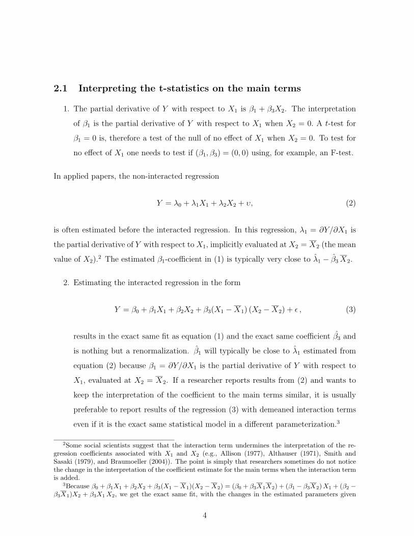
2.1 Interpreting the t-statistics on the main terms

1. The partial derivative of Y with respect to X1 is β1 + β3X2. The interpretation

of β1 is the partial derivative of Y with respect to X1 when X2 = 0. A t-test for

β1 = 0 is, therefore a test of the null of no effect of X1 when X2 = 0. To test for

no effect of X1 one needs to test if (β1, β3) = (0, 0) using, for example, an F-test.

In applied papers, the non-interacted regression

Y = λ0 + λ1X1 + λ2X2 + υ, (2)

is often estimated before the interacted regression. In this regression, λ1 = ∂Y/∂X1 is

the partial derivative of Y with respect to X1, implicitly evaluated at X2 = X2 (the mean

value of X2).2 The estimated β1-coefficient in (1) is typically very close to λ̂1 − β̂3X2.

2. Estimating the interacted regression in the form

Y = β0 + β1X1 + β2X2 + β3(X1 −X1) (X2 −X2) + ε , (3)

results in the exact same fit as equation (1) and the exact same coefficient β̂3 and

is nothing but a renormalization. β̂1 will typically be close to λ̂1 estimated from

equation (2) because β1 = ∂Y/∂X1 is the partial derivative of Y with respect to

X1, evaluated at X2 = X2. If a researcher reports results from (2) and wants to

keep the interpretation of the coefficient to the main terms similar, it is usually

preferable to report results of the regression (3) with demeaned interaction terms

even if it is the exact same statistical model in a different parameterization.3

2Some social scientists suggest that the interaction term undermines the interpretation of the re-gression coefficients associated with X1 and X2 (e.g., Allison (1977), Althauser (1971), Smith andSasaki (1979), and Braumoeller (2004)). The point is simply that researchers sometimes do not noticethe change in the interpretation of the coefficient estimate for the main terms when the interaction termis added.

3Because β0 + β1X1 + β2X2 + β3(X1 −X1)(X2 −X2) = (β0 + β3X1X2) + (β1 − β3X2)X1 + (β2 −β3X1)X2 + β3X1X2, we get the exact same fit, with the changes in the estimated parameters given

4

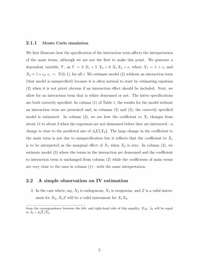
2.1.1 Monte Carlo simulation

We first illustrate how the specification of the interaction term affects the interpretation

of the main terms, although we are not the first to make this point. We generate a

dependent variable, Y , as Y = 3 X1 + 5 X2 + 8 X1X2 + ε, where X1 = 1 + ε1 and

X2 = 1 + ε2, εi ∼ N(0, 1), for all i. We estimate model (2) without an interaction term

(that model is misspecified) because it is often natural to start by estimating equation

(2) when it is not priori obvious if an interaction effect should be included. Next, we

allow for an interaction term that is either demeaned or not. The latter specifications

are both correctly specified. In column (1) of Table 1, the results for the model without

an interaction term are presented and, in columns (2) and (3), the correctly specified

model is estimated. In column (2), we see how the coefficient to X1 changes from

about 11 to about 3 when the regressors are not demeaned before they are interacted—a

change is close to the predicted size of β3E{X2}. The large change in the coefficient to

the main term is not due to misspecification but it reflects that the coefficient to X1

is to be interpreted as the marginal effect of X1 when X2 is zero. In column (3), we

estimate model (3) where the terms in the interaction are demeaned and the coefficient

to interaction term is unchanged from column (2) while the coefficients of main terms

are very close to the ones in column (1)—with the same interpretation.

2.2 A simple observation on IV estimation

3. In the case where, say, X2 is endogenous, X1 is exogenous, and Z is a valid instru-

ment for X2, X1Z will be a valid instrument for X1X2.

from the correspondence between the left- and right-hand side of this equality. E.g., λ̂0 will be equalto β̂0 + β3X1X2 .

5

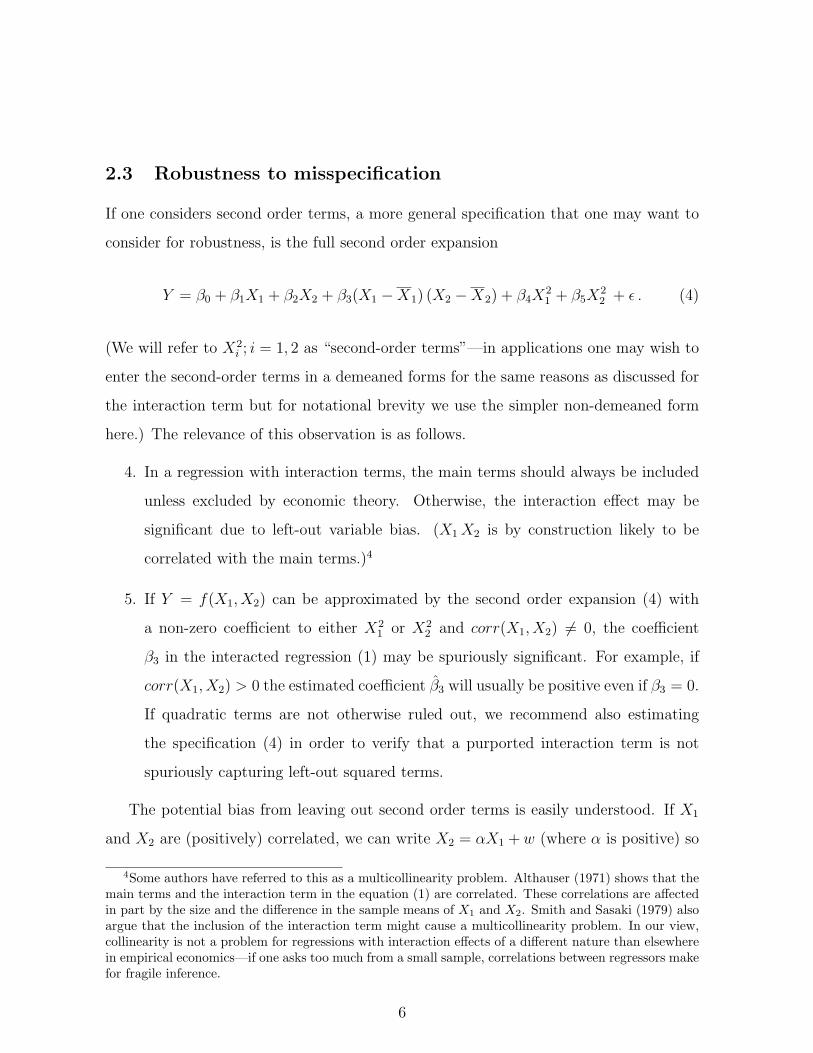
2.3 Robustness to misspecification

If one considers second order terms, a more general specification that one may want to

consider for robustness, is the full second order expansion

Y = β0 + β1X1 + β2X2 + β3(X1 −X1) (X2 −X2) + β4X21 + β5X

22 + ε . (4)

(We will refer to X2i ; i = 1, 2 as “second-order terms”—in applications one may wish to

enter the second-order terms in a demeaned forms for the same reasons as discussed for

the interaction term but for notational brevity we use the simpler non-demeaned form

here.) The relevance of this observation is as follows.

4. In a regression with interaction terms, the main terms should always be included

unless excluded by economic theory. Otherwise, the interaction effect may be

significant due to left-out variable bias. (X1X2 is by construction likely to be

correlated with the main terms.)4

5. If Y = f(X1, X2) can be approximated by the second order expansion (4) with

a non-zero coefficient to either X21 or X2

2 and corr(X1, X2) 6= 0, the coefficient

β3 in the interacted regression (1) may be spuriously significant. For example, if

corr(X1, X2) > 0 the estimated coefficient β̂3 will usually be positive even if β3 = 0.

If quadratic terms are not otherwise ruled out, we recommend also estimating

the specification (4) in order to verify that a purported interaction term is not

spuriously capturing left-out squared terms.

The potential bias from leaving out second order terms is easily understood. If X1

and X2 are (positively) correlated, we can write X2 = αX1 +w (where α is positive) so

4Some authors have referred to this as a multicollinearity problem. Althauser (1971) shows that themain terms and the interaction term in the equation (1) are correlated. These correlations are affectedin part by the size and the difference in the sample means of X1 and X2. Smith and Sasaki (1979) alsoargue that the inclusion of the interaction term might cause a multicollinearity problem. In our view,collinearity is not a problem for regressions with interaction effects of a different nature than elsewherein empirical economics—if one asks too much from a small sample, correlations between regressors makefor fragile inference.

6

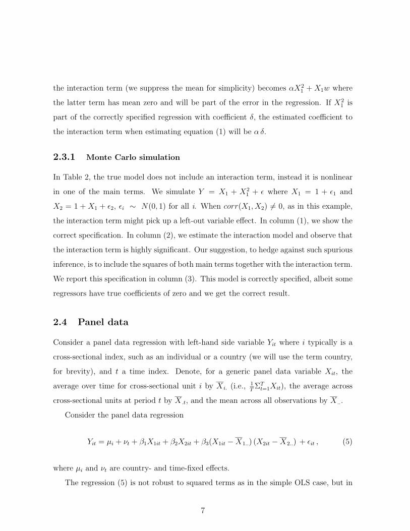
the interaction term (we suppress the mean for simplicity) becomes αX21 + X1w where

the latter term has mean zero and will be part of the error in the regression. If X21 is

part of the correctly specified regression with coefficient δ, the estimated coefficient to

the interaction term when estimating equation (1) will be α δ.

2.3.1 Monte Carlo simulation

In Table 2, the true model does not include an interaction term, instead it is nonlinear

in one of the main terms. We simulate Y = X1 + X21 + ε where X1 = 1 + ε1 and

X2 = 1 + X1 + ε2, εi ∼ N(0, 1) for all i. When corr(X1, X2) 6= 0, as in this example,

the interaction term might pick up a left-out variable effect. In column (1), we show the

correct specification. In column (2), we estimate the interaction model and observe that

the interaction term is highly significant. Our suggestion, to hedge against such spurious

inference, is to include the squares of both main terms together with the interaction term.

We report this specification in column (3). This model is correctly specified, albeit some

regressors have true coefficients of zero and we get the correct result.

2.4 Panel data

Consider a panel data regression with left-hand side variable Yit where i typically is a

cross-sectional index, such as an individual or a country (we will use the term country,

for brevity), and t a time index. Denote, for a generic panel data variable Xit, the

average over time for cross-sectional unit i by X i. (i.e., 1T

ΣTt=1Xit), the average across

cross-sectional units at period t by X .t, and the mean across all observations by X ...

Consider the panel data regression

Yit = µi + νt + β1X1it + β2X2it + β3(X1it −X1..) (X2it −X2..) + εit , (5)

where µi and νt are country- and time-fixed effects.

The regression (5) is not robust to squared terms as in the simple OLS case, but in

7

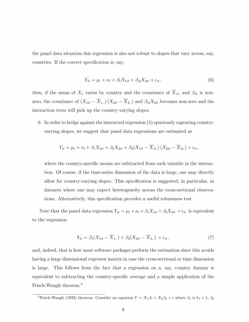
the panel data situation this regression is also not robust to slopes that vary across, say,

countries. If the correct specification is, say,

Yit = µi + νt + β1X1it + βi2X2it + εit , (6)

then, if the mean of X1 varies by country and the covariance of X1i. and βi2 is non-

zero, the covariance of (X1it −X1..) (X2it −X2..) and βi2X2it becomes non-zero and the

interaction term will pick up the country-varying slopes.

6. In order to hedge against the interacted regression (5) spuriously capturing country-

varying slopes, we suggest that panel data regressions are estimated as

Yit = µi + νt + β1X1it + β2X2it + β3(X1it −X1i.) (X2it −X2i.) + εit ,

where the country-specific means are subtracted from each variable in the interac-

tion. Of course, if the time-series dimension of the data is large, one may directly

allow for country-varying slopes. This specification is suggested, in particular, in

datasets where one may expect heterogeneity across the cross-sectional observa-

tions. Alternatively, this specification provides a useful robustness test.

Note that the panel data regression Yit = µi + νt +β1X1it +β2X2it + εit is equivalent

to the regression

Yit = β1(X1it −X1..) + β2(X2it −X2..) + εit , (7)

and, indeed, that is how most software packages perform the estimation since this avoids

having a large dimensional regressor matrix in case the cross-sectional or time dimension

is large. This follows from the fact that a regression on a, say, country dummy is

equivalent to subtracting the country-specific average and a simple application of the

Frisch-Waugh theorem.5

5Frisch-Waugh (1933) theorem: Consider an equation Y = X1β1 +X2β2 + ε where β1 is k1 × 1, β2

8

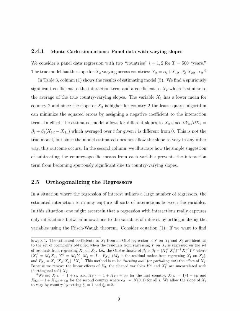
2.4.1 Monte Carlo simulations: Panel data with varying slopes

We consider a panel data regression with two “countries” i = 1, 2 for T = 500 “years.”

The true model has the slope forX2 varying across countries: Yit = αi+X1it+ξi X2it+εit.6

In Table 3, column (1) shows the results of estimating model (5). We find a spuriously

significant coefficient to the interaction term and a coefficient to X2 which is similar to

the average of the true country-varying slopes. The variable X1 has a lower mean for

country 2 and since the slope of X2 is higher for country 2 the least squares algorithm

can minimize the squared errors by assigning a negative coefficient to the interaction

term. In effect, the estimated model allows for different slopes to X2 since ∂Yit/∂X2 =

β2 + β3(X1it−X1..) which averaged over t for given i is different from 0. This is not the

true model, but since the model estimated does not allow the slope to vary in any other

way, this outcome occurs. In the second column, we illustrate how the simple suggestion

of subtracting the country-specific means from each variable prevents the interaction

term from becoming spuriously significant due to country-varying slopes.

2.5 Orthogonalizing the Regressors

In a situation where the regression of interest utilizes a large number of regressors, the

estimated interaction term may capture all sorts of interactions between the variables.

In this situation, one might ascertain that a regression with interactions really captures

only interactions between innovations to the variables of interest by orthogonalizing the

variables using the Frisch-Waugh theorem. Consider equation (1). If we want to find

is k2 × 1. The estimated coefficients to X1 from an OLS regression of Y on X1 and X2 are identicalto the set of coefficients obtained when the residuals from regressing Y on X2 is regressed on the setof residuals from regressing X1 on X2. I.e., the OLS estimate of β1 is β̂1 = (Xψ ′

1 Xψ1 )−1Xψ ′

1 Y ψ where(Xψ

1 = M2X1, Yψ = M2 Y, M2 = [I − PX2 ] (M2 is the residual maker from regressing X1 on X2),

and PX2 = X2 (X2′X2)−1X2

′. This method is called “netting out” (or partialing out) the effect of X2.

Because we remove the linear effects of X2, the cleaned variables Y ψ and Xψ1 are uncorrelated with

(“orthogonal to”) X2.6We set X11t = 1 + ε1t and X21t = 1 + X11t + ε2t for the first country, X12t = 1/4 + ε3t and

X22t = 1 + X12t + ε4t for the second country where εit ∼ N(0, 1) for all i. We allow the slope of X2

to vary by country by setting ξ1 = 1 and ξ2 = 2.

9

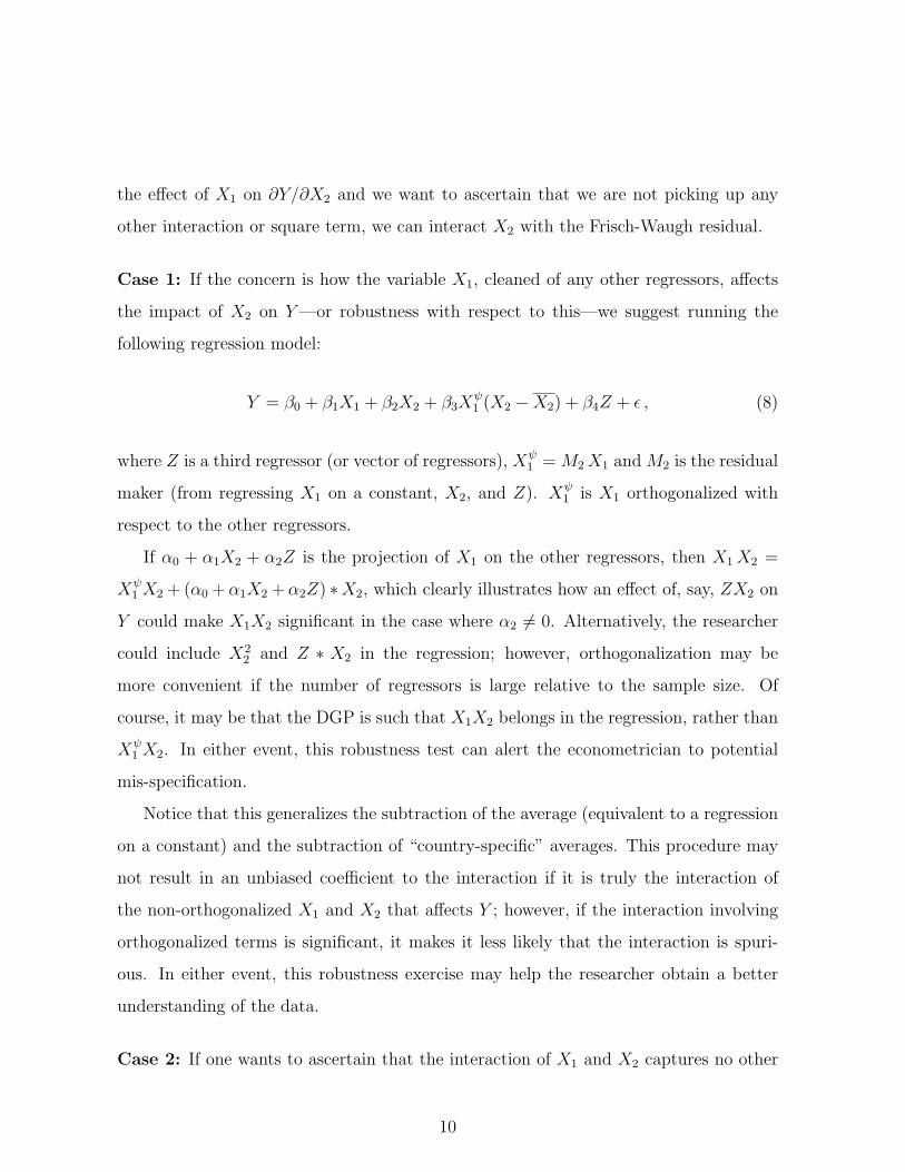
the effect of X1 on ∂Y/∂X2 and we want to ascertain that we are not picking up any

other interaction or square term, we can interact X2 with the Frisch-Waugh residual.

Case 1: If the concern is how the variable X1, cleaned of any other regressors, affects

the impact of X2 on Y—or robustness with respect to this—we suggest running the

following regression model:

Y = β0 + β1X1 + β2X2 + β3Xψ1 (X2 −X2) + β4Z + ε , (8)

where Z is a third regressor (or vector of regressors), Xψ1 = M2X1 and M2 is the residual

maker (from regressing X1 on a constant, X2, and Z). Xψ1 is X1 orthogonalized with

respect to the other regressors.

If α0 + α1X2 + α2Z is the projection of X1 on the other regressors, then X1X2 =

Xψ1 X2 + (α0 + α1X2 + α2Z) ∗X2, which clearly illustrates how an effect of, say, ZX2 on

Y could make X1X2 significant in the case where α2 6= 0. Alternatively, the researcher

could include X22 and Z ∗ X2 in the regression; however, orthogonalization may be

more convenient if the number of regressors is large relative to the sample size. Of

course, it may be that the DGP is such that X1X2 belongs in the regression, rather than

Xψ1 X2. In either event, this robustness test can alert the econometrician to potential

mis-specification.

Notice that this generalizes the subtraction of the average (equivalent to a regression

on a constant) and the subtraction of “country-specific” averages. This procedure may

not result in an unbiased coefficient to the interaction if it is truly the interaction of

the non-orthogonalized X1 and X2 that affects Y ; however, if the interaction involving

orthogonalized terms is significant, it makes it less likely that the interaction is spuri-

ous. In either event, this robustness exercise may help the researcher obtain a better

understanding of the data.

Case 2: If one wants to ascertain that the interaction of X1 and X2 captures no other

10

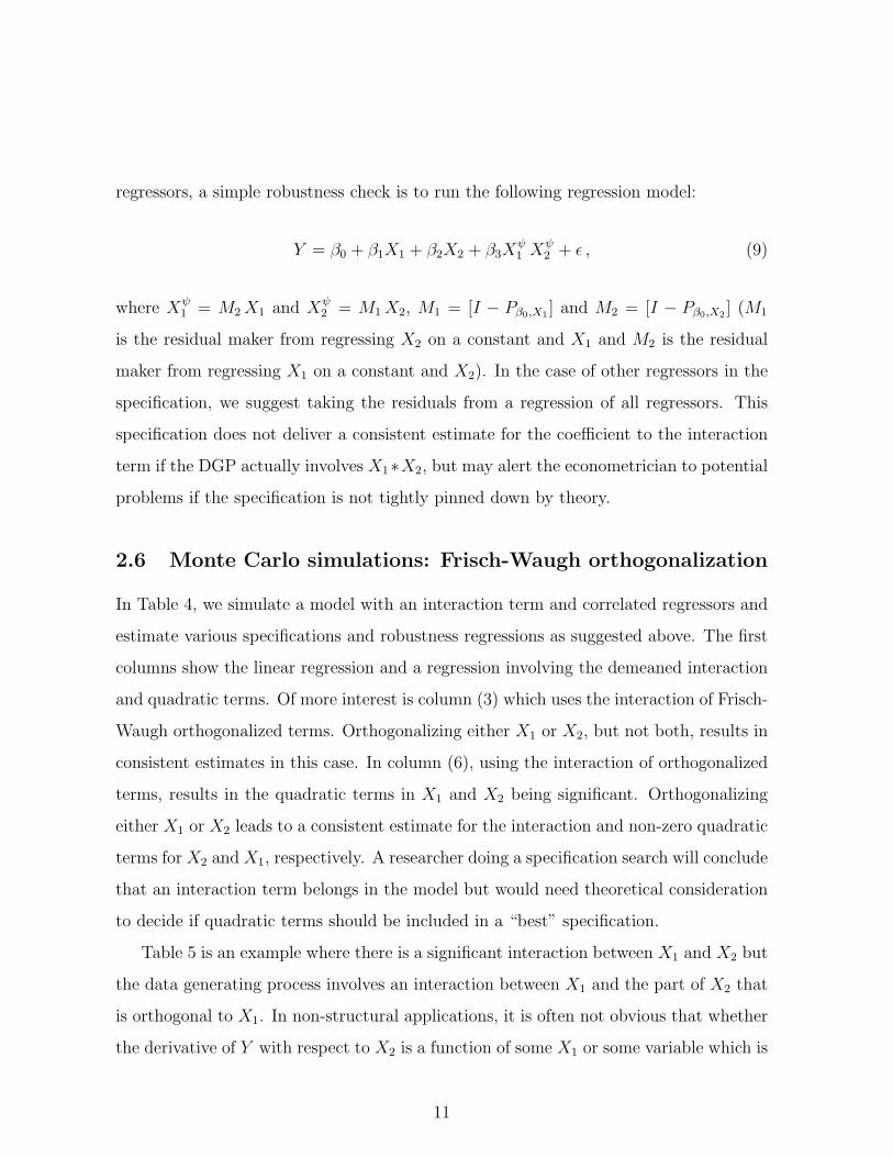
regressors, a simple robustness check is to run the following regression model:

Y = β0 + β1X1 + β2X2 + β3Xψ1 X

ψ2 + ε , (9)

where Xψ1 = M2X1 and Xψ

2 = M1X2, M1 = [I − Pβ0,X1 ] and M2 = [I − Pβ0,X2 ] (M1

is the residual maker from regressing X2 on a constant and X1 and M2 is the residual

maker from regressing X1 on a constant and X2). In the case of other regressors in the

specification, we suggest taking the residuals from a regression of all regressors. This

specification does not deliver a consistent estimate for the coefficient to the interaction

term if the DGP actually involves X1∗X2, but may alert the econometrician to potential

problems if the specification is not tightly pinned down by theory.

2.6 Monte Carlo simulations: Frisch-Waugh orthogonalization

In Table 4, we simulate a model with an interaction term and correlated regressors and

estimate various specifications and robustness regressions as suggested above. The first

columns show the linear regression and a regression involving the demeaned interaction

and quadratic terms. Of more interest is column (3) which uses the interaction of Frisch-

Waugh orthogonalized terms. Orthogonalizing either X1 or X2, but not both, results in

consistent estimates in this case. In column (6), using the interaction of orthogonalized

terms, results in the quadratic terms in X1 and X2 being significant. Orthogonalizing

either X1 or X2 leads to a consistent estimate for the interaction and non-zero quadratic

terms for X2 and X1, respectively. A researcher doing a specification search will conclude

that an interaction term belongs in the model but would need theoretical consideration

to decide if quadratic terms should be included in a “best” specification.

Table 5 is an example where there is a significant interaction between X1 and X2 but

the data generating process involves an interaction between X1 and the part of X2 that

is orthogonal to X1. In non-structural applications, it is often not obvious that whether

the derivative of Y with respect to X2 is a function of some X1 or some variable which is

11

part of X1. For example, if the effect of credit varies by industry, it may not be “indus-

try” (the type of product made) that matters but the correlation of industry dummies

with financial structure. In the example here, the regressions where X2 is Frisch-Waugh

orthogonalized deliver consistent estimates while the regular interaction, still significant,

does not—neither does the specification with both terms orthogonalized. The specifica-

tion in column (5) is the true model. An investigator searching for specifications would

notice the high t-value for the interaction term in this specification. The quadratic term

in X2 in column (7) is also very significant so an investigator would need to invoke the-

oretical considerations to choose between specifications—our suggested robustness tests

do not substitute for this. They do, however, flag potential issues which the practice of

reporting only a regression with X1, X2, and X1 ∗X2 does not.

Table 6 simulates a model with a data generating process which is quadratic in X1

while X1 and X2 are correlated. In this case, the interaction term will be spuriously

significant unless quadratic terms are included or either X2 or both of the independent

variables have been orthogonalized. Our suggestion is to include quadratic terms but

this may be impractical in the case of a large amount of regressors in which case the

orthogonalized regressions may be substitutes.

3 Replications

We replicate five important papers and examine if their implementation of interaction

effects are robust. (Data details are given in the appendix.) First, in Table 7, we ex-

amine if the results of the highly influential paper of Rajan and Zingales (1998) are

robust. The conclusion of this paper, which has by early 2010 has almost 2500 refer-

ences, is that accounting standards matters—in particular in industries that are highly

dependent on finance. Considering the influence of the paper, it is important to exam-

ine if the results are robust. The interactions of interest are between sectors’ external

financial dependence (E) and the country-level indicators of finance availability: the

12

ratio of (total equity market capitalization plus domestic credit) to GDP (T ) and ac-

counting standards (A). We examine if the results are robust to using Frisch-Waugh

residuals for total capitalization (T ) and accounting standards (A). We find that using

Frisch-Waugh residuals in the interaction term strengthens the size and significance of

the interactions; in fact, the interaction of external dependence and equity market capi-

talization and credit turns from insignificant to clearly significant at the 5-percent level

with the expected sign. Our robustness exercise makes the original claims of Rajan and

Zingales (1998) empirically more convincing.

We also briefly consider the results of Rajan and Zingales (2003), who examined if the

number of listed firms in a country is affected by openness (O), the historical (1913) level

of industrialization (I), and the interaction of openness and historical industrialization.

From Table 8, we see that the t-statistic on the main terms are very much affected by the

interaction terms not being centered although this only involves a different interpretation

of the t-statistic which are positive and significant when the variables are centered in

the interaction. The impact of the interaction term is very robust to including quadratic

terms in the main variables or orthogonalizing the regressors (indicating that these were

likely to be near-orthogonal to begin with). Overall, the conclusions of Rajan and

Zingales (2003) are robust to the potential misspecifications that we suggest examining.

Castro, Clementi, and MacDonald (2004) hypothesize that strengthening of prop-

erty rights, as measured by laws mandating “one share-one vote,” “anti-director rights”

(which limit the power of directors to extract surplus), “creditor rights,” and “rule of

law,” are beneficial for growth and more so when restrictions on capital transactions

(capital flows) are weaker. They examine this by including interaction terms between

the property rights indices and capital restrictions. Table 9 replicates Table 1 of their

paper. We do not display regressions with centered interactions because the interaction

terms are the variables of interest. In column (2), quadratic terms for the property

rights measures are included but this strengthens the authors’ main result of negative

interactions. In column (3), we include a quadratic term in log GDP, to which weak-

13

ens the significance of the parameters of interest below standard significance but we

do not further explore this issue which is not at the focus of this article.7 If we use

Frisch-Waugh residuals for either the creditor rights measures of the capital restrictions

measure we again find that the estimated interactions are mainly negative. Overall, the

point estimates in the Castro, Clementi, and MacDonald (2004) study are not all robust,

as one might conjecture from the size of the t-statistics, but the overall message of their

regressions appears very robust to the kind of robustness checks we recommend.

Caprio, Laeven, and Levine (2007) examine if bank valuations (relative to book

values) are higher where owners have stronger rights (Rights), as measured by an anti-

director index, and whether this result is stronger when a larger share of cash flows (CF )

accrues to the owners. The first column of Table 10 replicates Table 5 (column 1) of

Caprio, Laeven, and Levine (2007). Column (2) includes quadratic terms and centers

the variables before interacting. The very large t-statistic found for the main term,

“rights”, in column 1 turns insignificant and both main variables change signs. The

non-centered implementation of Caprio, Laeven, and Levine (2007), in our opinion,

gives a potentially misleading impression of the effect of the main terms; for example,

the t-statistic of “rights” in column 1 implies that there is large significant effect of

ownership rights on valuation when owners’ cash-flow share is nil. But a cash-flow share

of nil is meaningless. Better news for the published paper is that the interaction terms

which are the authors’ main focus clearly are robustly estimated.

Finally, in Table 11, we explore a specific set of results from Spilimbergo (2009), that

the interaction of “students abroad” with “democracy in host country” has a negative

effect on the Polity2 measure of democracy.8 This is a panel-data analysis (country by

time) with both time- and country-fixed effects which implies that the coefficients to

7The dateset used Castro, Clementi, and MacDonald (2004) is fairly small—45 observations—andsome non-robustness must be expected. A fair discussion of the validity of their results would involvea much longer discussion.

8We choose this article because it is an example of panel data regression for which the data are easilyavailable; however, the results we replicate are just one of a set of estimations in Spilimbergo’s (2009)article so the discussion here should be seen as an example rather than an examination of the centralmessage of Spilimbergo’s paper.

14

the main terms, are determined by these variable after country and time means have

been subtracted. We ask if the results are robust to potentially country-varying slopes

to the main terms by removing country-specific averages before interacting. The first

column shows the results reported in Spilimbergo (2009) while the second column repli-

cates the analysis using the data posted by Spilimbergo on the web site of the American

Economic Review—we need both, in order to ascertain that any deviation between our

results and the results in the American Economic Review is not due the discrepancy

between the posted data and the data actually used by Spilimbergo. The results are

very similar between those columns except the R-square is much higher using the posted

data. In column (3), we show the results using interactions that are demeaned country-

by-country. The results are clearly not robust to this alternative specification—the coef-

ficient to (non-interacted) “students abroad” becomes insignificant while the coefficient

to the interaction changes from significantly negative to (nearly significantly) positive.

Within the setting of our paper, it will take us too far afield to discuss in detail whether

country-varying slopes in this setting is a reasonable alternative empirical specification

for Spilimbergo’s study, although it does not seem far fetched that growth of, say, democ-

racy, varies across countries. Our main point is that, in general, in panel studies using

data from heterogenous cross-sectional units it may be a reasonable alternative (unless

rules out by theory) and it will often be reasonable to examine robustness against this

alternative.

4 Conclusions

We provide practical advice regarding interpretation and robustness of models with

interaction terms for econometric practitioners—in particular, we suggest some simple

rules-of-thumb intended to minimize the risk of estimated interaction terms spuriously

capturing other features of the data. The main tenet of our results is that researchers

applying interaction terms should be very careful with specification and interpretation

15

and not just put X1X2 into a regression equation without considering robustness of

results to functional form.

16

Appendix—Notes on data collection

Rajan and Zingales (1998):

The data is downloaded from Luigi Zingales’ home page. The dependent variable is

the annual compounded growth rate in real value added for each ISIC industry in each

country for the period 1980–1990. External dependence (E) is the fraction of capital

expenditures not financed with internal funds for firms in the United States in the same

industry between 1980 and 1990. Total capitalization (T ) is the ratio of (equity market

capitalization plus domestic credit) to GDP. Accounting standards (A) is a country-level

index developed by the Center for International Financial Analysis and Research rank-

ing the amount of disclosure in annual company reports. I is industry’s share of total

value added in manufacturing in 1980 is from the United Nations Statistics. For more

details on data sources, see Rajan and Zingales (1998).

Rajan and Zingales (2003):

We collected the data using the sources given in Rajan and Zingales (2003). The

dependent variable, number of companies to population, is the ratio of the number of

domestic companies whose equity is publicly traded in a domestic stock exchange to

population in millions in 1993 (it is used as an indicator of the importance of equity

markets). As a first source, stock exchange handbooks are used to count the number

of companies and the Bulletin of the International Institute of Statistics is used as a

second source. The countries in the sample are Australia, Austria, Belgium, Brazil,

Canada, Denmark, France, Germany, India, Italy, Japan, the Netherlands, Norway,

Russia, Sweden, Switzerland, the UK, and the United States.

GDP is Gross Domestic Product in 1913 obtained from International Historical

Statistics (Mitchell, 1995). We could not find this series for Russia and we used fig-

ure 2 in Rajan and Zingales (2003) to interpolate the data. Openness (O) is the sum

of exports and imports of goods in 1913 divided by GDP in 1913. Exports and imports

17

are from the Statistical Yearbook of the League of Nations.9 For Brazil and Russia, we

could not find export and import data and we interpolated them from the averages of

the variables in Rajan and Zingales (2003)’s Table 6.

Per capita industrialization (I) is the index of industrialization by country in 1913

as computed by Bairoch (1982). For more details about data sources, see Rajan and

Zingales (2003).

Castro, Clementi, and MacDonald (2004):

We collected the data using the sources given in Castro, Clementi, and MacDon-

ald (2004). The dependent variable is the average annual growth rate of real GDP

per worker 1967-1996. Real GDP per worker is from the Penn World Tables, version

6.1. The set of countries corresponds to the 49 countries in La Porta, Lopez-de-Silanes,

Shleifer, and Vishny (1998) except we do not have data for Germany, Jordan, Venezuela,

Switzerland, Zimbabwe, and Taiwan. Castro, Clementi, and MacDonald (2004) use four

of the indicators of nvestor protection introduced by La Porta, Lopez-de-Silanes, Shleifer,

and Vishny (1998). The variable CR is an index aggregating different creditor rights

in firm reorganization and liquidation upon default. The indicator antidirector rights

(AR), and the dummy one share-one vote (OV ), are two indices of shareholder rights

geared towards measuring the ability of small shareholders to participate in decision

making. Finally, the index rule of law (RL), proxies for the quality of law enforcement.

These variables are described in more details in La Porta, Lopez-de-Silanes, Shleifer,

and Vishny (1998. (1998).

RCT is a variable created to measure restrictions on capital transactions. First,

a time-series dummy is constructed based on the IMF’s Annual Report on Exchange

Arrangements and Exchange Restrictions. The dummy variable takes the value of 1 for

a given country in a given year if the IMF finds evidence of restrictions on payments

on capital transactions for that country-year. Such restrictions include both taxes and

9See http : //www.library.northwestern.edu/govpub/collections/leaque/stat.html.

18

quantity restrictions on the trade of foreign assets. Second, we compute RCT as the

average of this dummy over the sample period to obtain a measure of the fraction of

time each country imposed restrictions on international capital transactions.

Caprio, Laeven, and Levine (2007):

The exact data is used in Caprio, Laeven, and Levine (2007) and is downloaded from

Ross Levine’s home-page. It is a new database on bank ownership around the world

and constructed by Caprio, Laeven, and Levine (2007). Market-to-book is the market

to book value of each bank’s equity of a bank from Bankscope database published in

2003.10 In other words, it is the ratio of the market value of equity to the book value

of equity. Loan Growth (LG) is each bank’s average net loan growth during the last 3

years from Bankscope published in 2003.

Rights is an index of anti-director rights for the country from La Porta, Lopez-de-

Silanes, Shleifer, and Vishny (2002). The range for the index is from zero to six formed

by adding by adding the number of times each of the following conditions hold: (1) the

country allows shareholders to mail their proxy vote, (2) shareholders are not required

to deposit their shares prior to the General Shareholders’ Meeting, (3) cumulative voting

or proportional representation of minorities on the board of directors is allowed, (4) an

oppressed minorities mechanism is in place, (5) the minimum percentage of share capital

that entitles a shareholder to call for an Extraordinary Shareholders’ Meeting is less than

or equal to 10 percent (the sample median), or (6) when shareholders have preemptive

rights that can only be waived by a shareholders meeting.

CF is the fraction of each bank’s ultimate cash-flow rights held by the controlling

owners. CF values are computed as the product of all the equity stakes along the con-

trol chain. The controlling shareholder may hold cash-flow rights directly (i.e., through

shares registered in her name) and indirectly (i.e., through shares held by entities that, in

10Bankscope, maintained by Bureau van Dijk, contains financial and ownership information for about4,000 major banks.

19

turn, she controls). If there is a control chain, then we use the products of the cash-flow

rights along the chain. To compute the controlling shareholders total cash-flow rights

we sum direct and all indirect cash-flow rights.11 See Caprio, Laeven, and Levine (2007)

for more details on data sources.

Spilimbergo (2009):

The exact data is used in Spilimbergo (2009) and is available from the American

Economic Review’s web site. It is a unique panel data set of foreign students. The

data forms an unbalanced panel comprising five year intervals between 1955 and 2000.

The dependent variable, Polity2, is an index of democracy. StudentsAbroad (S) is the

share of foreign students over population and Democracy in host countries (DH) is the

average democracy index in host countries. See Spilimbergo (2009) for more details on

data sources.

11Caprio, Laeven, and Levine (2007)’s calculations are based on Bankscope, Worldscope, the Bankers’Almanac, 20-F filings, and company web sites.

20

References

Allison, Paul D. (1977), “Testing For Interaction in Multiple Regression,” AmericanJournal of Sociology 83, 144–153.

Althauser, Robert (1971), “Multicollinearity and Non-Additive Regression Models,” 453–472 in H. M. Blalock, Jr.(ed). Causal Models in the Social Sciences, Chicago:Aldine-Atherton.

Bairoch, Paul (1982), “International Industrialization levels from 1750 to 1980,” Jour-nal of European Economic History 11, 269–334.

Braumoeller, Bear F. (2004), “Hypothesis Testing and Multiplicative Interaction Terms,”International Organization 58, 807–820.

Burnside, Craig and David Dollar (2000), “Aid, Policies, and Growth,”American Eco-nomic Review 90, 847–868.

Caprio, Gerard, Luc Laeven, and Ross Levine (2007), “Governance and Bank Valuation,”Journal of Financial Intermediation 16, 584–617.

Castro, Rui, Gian Luca Clementi and Glenn MacDonald (2004), “Investor Protection, Op-timal Incentives, and Economic Growth,” Quarterly Journal of Economics 119,1131–1175.

Frisch, Ragnar and Frederick V. Waugh (1933), “Partial Time Regressions as Comparedwith Individual Trends,” Econometrica 1, 387-401.

Heston, Alan, Robert Summers, and Bettina Aten (2002), Penn World Table Version 6.1(Philadelphia, PA: Center for International Comparisons at the University of Penn-sylvania).

Knack, Stephen and Philip Keefer (1995), “Institutions and Economic Performance: Cross-Country Tests Using Alternative Institutional Measures,” Economics and Policies7, 207–227.

La Porta, Rafael, Florencio Lopez-de-Silanes, Andrei Shleifer, and Robert Vishny (1998),“Law and Finance,” Journal of Political Economy 106, 1113–1155.

La Porta, Rafael, Florencio Lopez-de-Silanes, Andrei Shleifer, and Robert Vishny (2002),“Investor Protection and Corporate Valuation,” Journal of Finance 57, 1147–1170.

Mitchell, Brian R. (1995), International Historical Statistics, Stockton Press, London.

Rajan, Raghuram G. and Luigi Zingales (1998), “Financial Dependence and Growth,”American Economic Review 88, 559–589.

21

Rajan, Raghuram G. and Luigi Zingales (2003), “The Great Reversals: The Politics ofFinancial Development in the Twentieth Century,” Journal of Financial Eco-nomics 69, 5–50.

Smith, Kent W. and M.S. Sasaki (1979), “Decreasing Multicollinearity: A Method forModels With Multiplicative Functions,” Sociological Methods and Research 8,35–56.

Spilimbergo, Antonio (2009), “Democracy and Foreign Education,” American EconomicReview 99, 528–543.

22

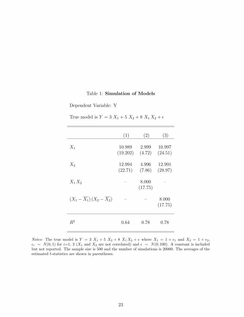
Table 1: Simulation of Models

Dependent Variable: Y

True model is Y = 3 X1 + 5 X2 + 8 X1X2 + ε

(1) (2) (3)

X1 10.989 2.999 10.997(19.202) (4.72) (24.51)

X2 12.994 4.996 12.991(22.71) (7.86) (28.97)

X1X2 – 8.000 –(17.75)

(X1 −X1) (X2 −X2) – – 8.000(17.75)

R2 0.64 0.78 0.78

Notes: The true model is Y = 3 X1 + 5 X2 + 8 X1X2 + ε where X1 = 1 + ε1 and X2 = 1 + ε2,εi ∼ N(0, 1) for i=1, 2 (X1 and X2 are not correlated) and ε ∼ N(0, 100). A constant is includedbut not reported. The sample size is 500 and the number of simulations is 20000. The averages of theestimated t-statistics are shown in parentheses.

23

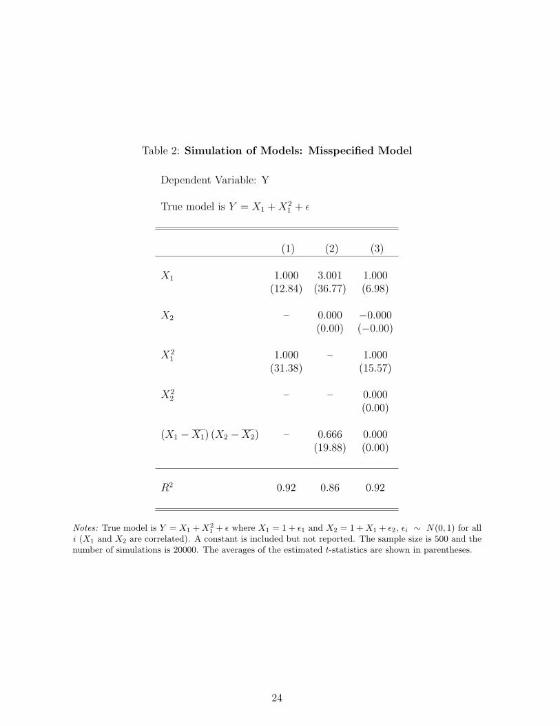
Table 2: Simulation of Models: Misspecified Model

Dependent Variable: Y

True model is Y = X1 +X21 + ε

(1) (2) (3)

X1 1.000 3.001 1.000(12.84) (36.77) (6.98)

X2 – 0.000 −0.000(0.00) (−0.00)

X21 1.000 – 1.000

(31.38) (15.57)

X22 – – 0.000

(0.00)

(X1 −X1) (X2 −X2) – 0.666 0.000(19.88) (0.00)

R2 0.92 0.86 0.92

Notes: True model is Y = X1 +X21 + ε where X1 = 1 + ε1 and X2 = 1 +X1 + ε2, εi ∼ N(0, 1) for all

i (X1 and X2 are correlated). A constant is included but not reported. The sample size is 500 and thenumber of simulations is 20000. The averages of the estimated t-statistics are shown in parentheses.

24

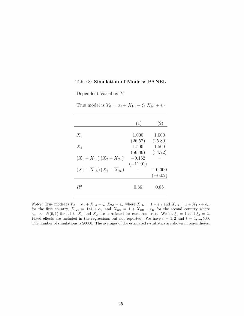
Table 3: Simulation of Models: PANEL

Dependent Variable: Y

True model is Yit = αi +X1it + ξi X2it + εit

(1) (2)

X1 1.000 1.000(26.57) (25.80)

X2 1.500 1.500(56.36) (54.72)

(X1 −X1..) (X2 −X2..) −0.152 –(−11.01)

(X1 −X1i.) (X2 −X2i.) – −0.000(−0.02)

R2 0.86 0.85

Notes: True model is Yit = αi + X1it + ξi X2it + εit where X11t = 1 + ε1t and X21t = 1 + X11t + ε2tfor the first country, X12t = 1/4 + ε3t and X22t = 1 + X12t + ε4t for the second country whereεit ∼ N(0, 1) for all i. X1 and X2 are correlated for each countries. We let ξ1 = 1 and ξ2 = 2.Fixed effects are included in the regressions but not reported. We have i = 1, 2 and t = 1, ..., 500.The number of simulations is 20000. The averages of the estimated t-statistics are shown in parentheses.

25

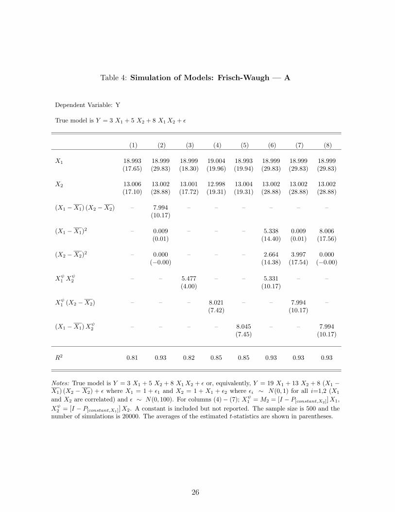
Table 4: Simulation of Models: Frisch-Waugh — A

Dependent Variable: Y

True model is Y = 3 X1 + 5 X2 + 8 X1X2 + ε

(1) (2) (3) (4) (5) (6) (7) (8)

X1 18.993 18.999 18.999 19.004 18.993 18.999 18.999 18.999(17.65) (29.83) (18.30) (19.96) (19.94) (29.83) (29.83) (29.83)

X2 13.006 13.002 13.001 12.998 13.004 13.002 13.002 13.002(17.10) (28.88) (17.72) (19.31) (19.31) (28.88) (28.88) (28.88)

(X1 −X1) (X2 −X2) – 7.994 – – – – – –(10.17)

(X1 −X1)2 – 0.009 – – – 5.338 0.009 8.006(0.01) (14.40) (0.01) (17.56)

(X2 −X2)2 – 0.000 – – – 2.664 3.997 0.000(−0.00) (14.38) (17.54) (−0.00)

Xψ1 X

ψ2 – – 5.477 – – 5.331 – –

(4.00) (10.17)

Xψ1 (X2 −X2) – – – 8.021 – – 7.994 –

(7.42) (10.17)

(X1 −X1)Xψ2 – – – – 8.045 – – 7.994

(7.45) (10.17)

R2 0.81 0.93 0.82 0.85 0.85 0.93 0.93 0.93

Notes: True model is Y = 3 X1 + 5 X2 + 8 X1X2 + ε or, equivalently, Y = 19 X1 + 13 X2 + 8 (X1 −X1) (X2 − X2) + ε where X1 = 1 + ε1 and X2 = 1 + X1 + ε2 where εi ∼ N(0, 1) for all i=1,2 (X1

and X2 are correlated) and ε ∼ N(0, 100). For columns (4)− (7); Xψ1 = M2 = [I − P[constant,X2]]X1,

Xψ2 = [I − P[constant,X1]]X2. A constant is included but not reported. The sample size is 500 and the

number of simulations is 20000. The averages of the estimated t-statistics are shown in parentheses.

26

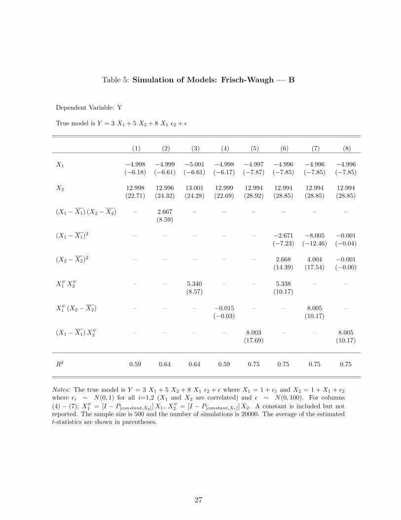
Table 5: Simulation of Models: Frisch-Waugh — B

Dependent Variable: Y

True model is Y = 3 X1 + 5 X2 + 8 X1 ε2 + ε

(1) (2) (3) (4) (5) (6) (7) (8)

X1 −4.998 −4.999 −5.001 −4.998 −4.997 −4.996 −4.996 −4.996(−6.18) (−6.61) (−6.61) (−6.17) (−7.87) (−7.85) (−7.85) (−7.85)

X2 12.998 12.996 13.001 12.999 12.994 12.994 12.994 12.994(22.71) (24.32) (24.28) (22.69) (28.92) (28.85) (28.85) (28.85)

(X1 −X1) (X2 −X2) – 2.667 – – – – – –(8.59)

(X1 −X1)2 – – – – – −2.671 −8.005 −0.001(−7.23) (−12.46) (−0.04)

(X2 −X2)2 – – – – – 2.668 4.004 −0.001(14.39) (17.54) (−0.00)

Xψ1 X

ψ2 – – 5.340 – – 5.338 – –

(8.57) (10.17)

Xψ1 (X2 −X2) – – – −0.015 – – 8.005 –

(−0.03) (10.17)

(X1 −X1)Xψ2 – – – – 8.003 – – 8.005

(17.69) (10.17)

R2 0.59 0.64 0.64 0.59 0.75 0.75 0.75 0.75

Notes: The true model is Y = 3 X1 + 5 X2 + 8 X1 ε2 + ε where X1 = 1 + ε1 and X2 = 1 + X1 + ε2where εi ∼ N(0, 1) for all i=1,2 (X1 and X2 are correlated) and ε ∼ N(0, 100). For columns(4) − (7); Xψ

1 = [I − P[constant,X2]]X1, Xψ2 = [I − P[constant,X1]]X2. A constant is included but not

reported. The sample size is 500 and the number of simulations is 20000. The average of the estimatedt-statistics are shown in parentheses.

27

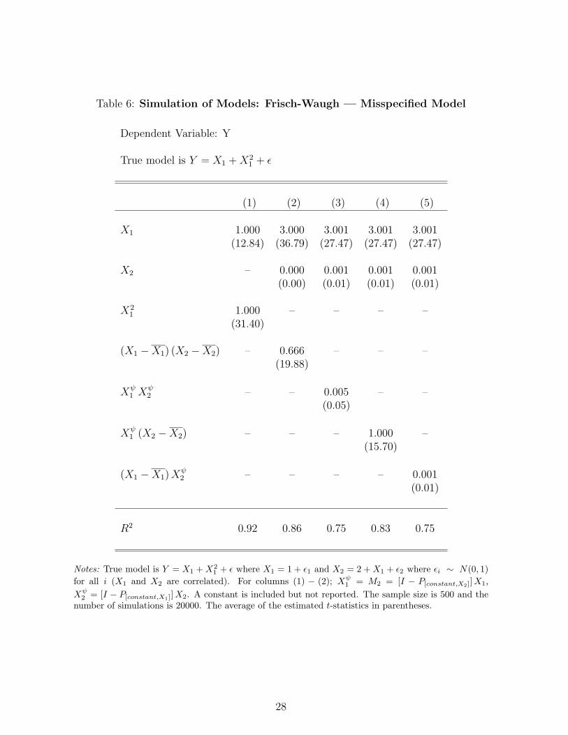
Table 6: Simulation of Models: Frisch-Waugh — Misspecified Model

Dependent Variable: Y

True model is Y = X1 +X21 + ε

(1) (2) (3) (4) (5)

X1 1.000 3.000 3.001 3.001 3.001(12.84) (36.79) (27.47) (27.47) (27.47)

X2 – 0.000 0.001 0.001 0.001(0.00) (0.01) (0.01) (0.01)

X21 1.000 – – – –

(31.40)

(X1 −X1) (X2 −X2) – 0.666 – – –(19.88)

Xψ1 X

ψ2 – – 0.005 – –

(0.05)

Xψ1 (X2 −X2) – – – 1.000 –

(15.70)

(X1 −X1)Xψ2 – – – – 0.001

(0.01)

R2 0.92 0.86 0.75 0.83 0.75

Notes: True model is Y = X1 +X21 + ε where X1 = 1 + ε1 and X2 = 2 +X1 + ε2 where εi ∼ N(0, 1)

for all i (X1 and X2 are correlated). For columns (1) − (2); Xψ1 = M2 = [I − P[constant,X2]]X1,

Xψ2 = [I − P[constant,X1]]X2. A constant is included but not reported. The sample size is 500 and the

number of simulations is 20000. The average of the estimated t-statistics in parentheses.

28

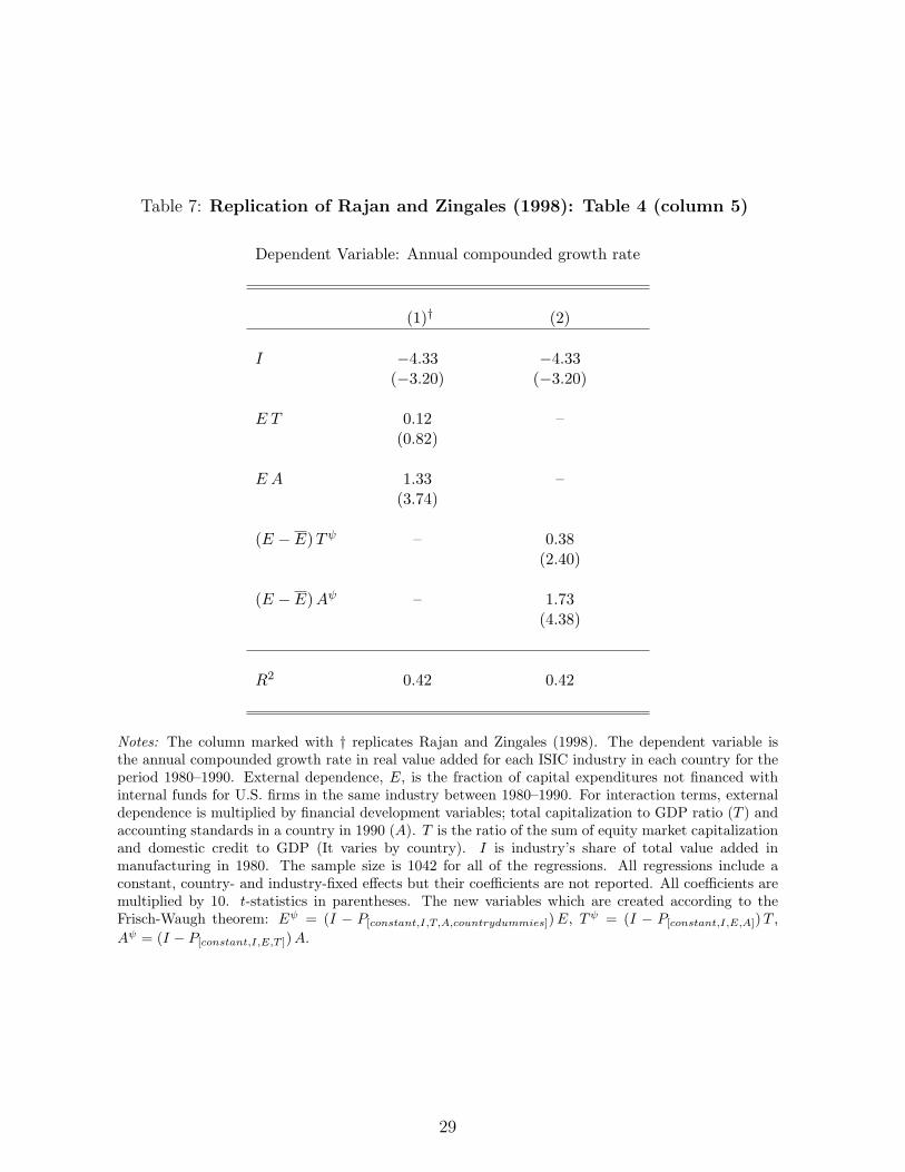
Table 7: Replication of Rajan and Zingales (1998): Table 4 (column 5)

Dependent Variable: Annual compounded growth rate

(1)† (2)

I −4.33 −4.33(−3.20) (−3.20)

E T 0.12 –(0.82)

E A 1.33 –(3.74)

(E − E)Tψ – 0.38(2.40)

(E − E)Aψ – 1.73(4.38)

R2 0.42 0.42

Notes: The column marked with † replicates Rajan and Zingales (1998). The dependent variable isthe annual compounded growth rate in real value added for each ISIC industry in each country for theperiod 1980–1990. External dependence, E, is the fraction of capital expenditures not financed withinternal funds for U.S. firms in the same industry between 1980–1990. For interaction terms, externaldependence is multiplied by financial development variables; total capitalization to GDP ratio (T ) andaccounting standards in a country in 1990 (A). T is the ratio of the sum of equity market capitalizationand domestic credit to GDP (It varies by country). I is industry’s share of total value added inmanufacturing in 1980. The sample size is 1042 for all of the regressions. All regressions include aconstant, country- and industry-fixed effects but their coefficients are not reported. All coefficients aremultiplied by 10. t-statistics in parentheses. The new variables which are created according to theFrisch-Waugh theorem: Eψ = (I − P[constant,I,T,A,countrydummies])E, Tψ = (I − P[constant,I,E,A])T ,Aψ = (I − P[constant,I,E,T ])A.

29

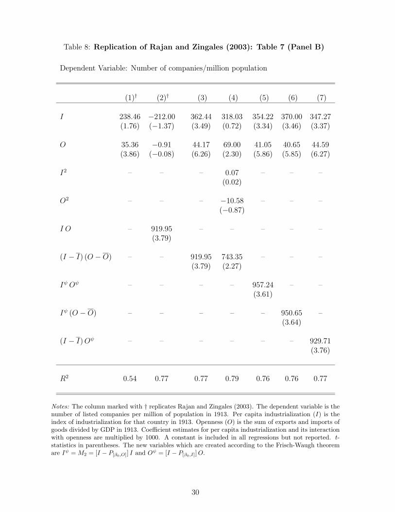
Table 8: Replication of Rajan and Zingales (2003): Table 7 (Panel B)

Dependent Variable: Number of companies/million population

(1)† (2)† (3) (4) (5) (6) (7)

I 238.46 −212.00 362.44 318.03 354.22 370.00 347.27(1.76) (−1.37) (3.49) (0.72) (3.34) (3.46) (3.37)

O 35.36 −0.91 44.17 69.00 41.05 40.65 44.59(3.86) (−0.08) (6.26) (2.30) (5.86) (5.85) (6.27)

I2 – – – 0.07 – – –(0.02)

O2 – – – −10.58 – – –(−0.87)

I O – 919.95 – – – – –(3.79)

(I − I) (O −O) – – 919.95 743.35 – – –(3.79) (2.27)

Iψ Oψ – – – – 957.24 – –(3.61)

Iψ (O −O) – – – – – 950.65 –(3.64)

(I − I)Oψ – – – – – – 929.71(3.76)

R2 0.54 0.77 0.77 0.79 0.76 0.76 0.77

Notes: The column marked with † replicates Rajan and Zingales (2003). The dependent variable is thenumber of listed companies per million of population in 1913. Per capita industrialization (I) is theindex of industrialization for that country in 1913. Openness (O) is the sum of exports and imports ofgoods divided by GDP in 1913. Coefficient estimates for per capita industrialization and its interactionwith openness are multiplied by 1000. A constant is included in all regressions but not reported. t-statistics in parentheses. The new variables which are created according to the Frisch-Waugh theoremare Iψ = M2 = [I − P[β0,O]] I and Oψ = [I − P[β0,I]]O.

30

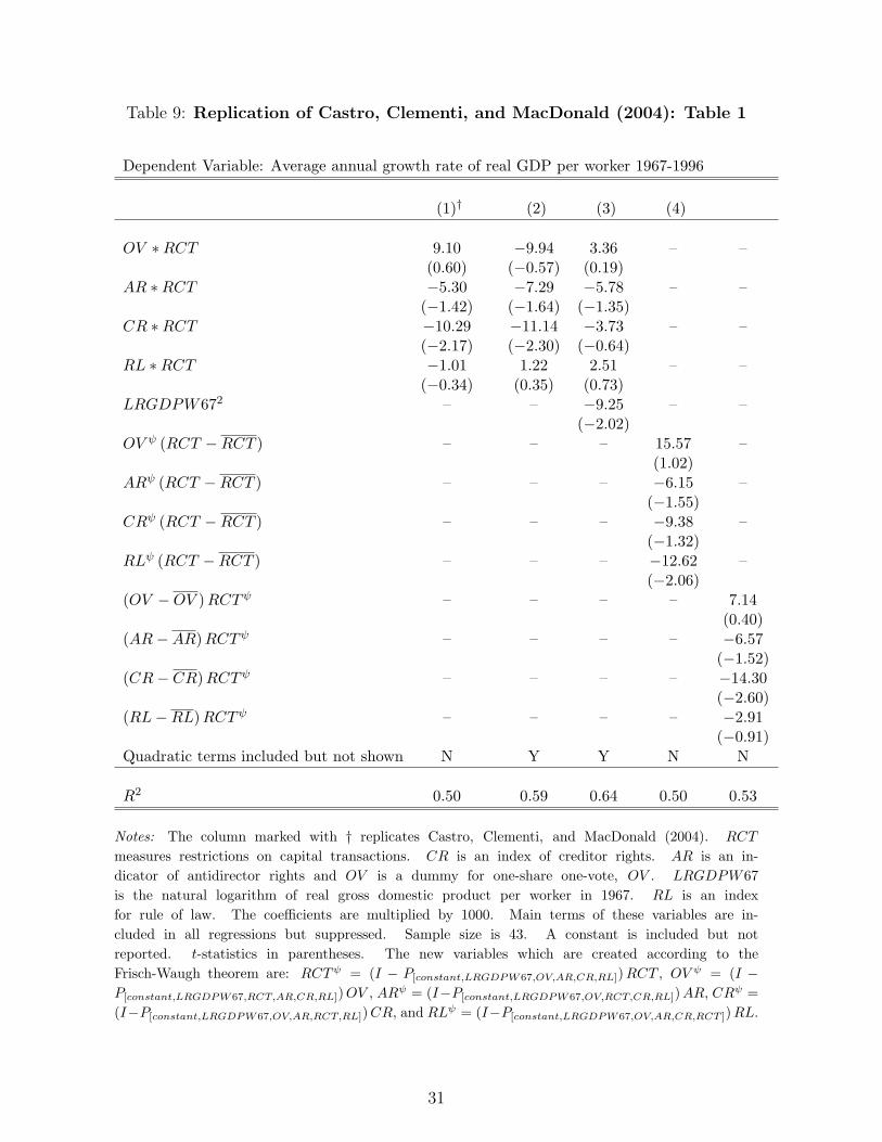
Table 9: Replication of Castro, Clementi, and MacDonald (2004): Table 1

Dependent Variable: Average annual growth rate of real GDP per worker 1967-1996

(1)† (2) (3) (4)

OV ∗RCT 9.10 −9.94 3.36 – –(0.60) (−0.57) (0.19)

AR ∗RCT −5.30 −7.29 −5.78 – –(−1.42) (−1.64) (−1.35)

CR ∗RCT −10.29 −11.14 −3.73 – –(−2.17) (−2.30) (−0.64)

RL ∗RCT −1.01 1.22 2.51 – –(−0.34) (0.35) (0.73)

LRGDPW672 – – −9.25 – –(−2.02)

OV ψ (RCT −RCT ) – – – 15.57 –(1.02)

ARψ (RCT −RCT ) – – – −6.15 –(−1.55)

CRψ (RCT −RCT ) – – – −9.38 –(−1.32)

RLψ (RCT −RCT ) – – – −12.62 –(−2.06)

(OV −OV )RCTψ – – – – 7.14(0.40)

(AR−AR)RCTψ – – – – −6.57(−1.52)

(CR− CR)RCTψ – – – – −14.30(−2.60)

(RL−RL)RCTψ – – – – −2.91(−0.91)

Quadratic terms included but not shown N Y Y N N

R2 0.50 0.59 0.64 0.50 0.53

Notes: The column marked with † replicates Castro, Clementi, and MacDonald (2004). RCT

measures restrictions on capital transactions. CR is an index of creditor rights. AR is an in-dicator of antidirector rights and OV is a dummy for one-share one-vote, OV . LRGDPW67is the natural logarithm of real gross domestic product per worker in 1967. RL is an indexfor rule of law. The coefficients are multiplied by 1000. Main terms of these variables are in-cluded in all regressions but suppressed. Sample size is 43. A constant is included but notreported. t-statistics in parentheses. The new variables which are created according to theFrisch-Waugh theorem are: RCTψ = (I − P[constant,LRGDPW67,OV,AR,CR,RL])RCT , OV ψ = (I −P[constant,LRGDPW67,RCT,AR,CR,RL])OV , ARψ = (I−P[constant,LRGDPW67,OV,RCT,CR,RL])AR, CRψ =(I−P[constant,LRGDPW67,OV,AR,RCT,RL])CR, and RLψ = (I−P[constant,LRGDPW67,OV,AR,CR,RCT ])RL.

31

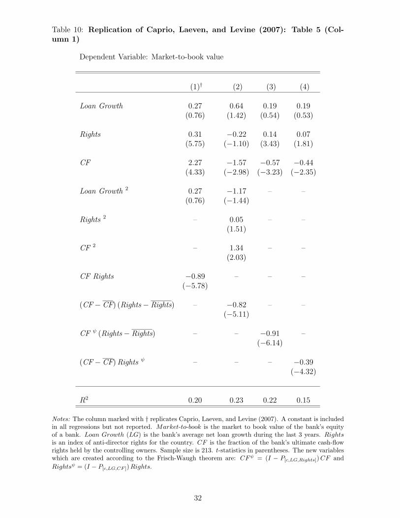
Table 10: Replication of Caprio, Laeven, and Levine (2007): Table 5 (Col-umn 1)

Dependent Variable: Market-to-book value

(1)† (2) (3) (4)

Loan Growth 0.27 0.64 0.19 0.19(0.76) (1.42) (0.54) (0.53)

Rights 0.31 −0.22 0.14 0.07(5.75) (−1.10) (3.43) (1.81)

CF 2.27 −1.57 −0.57 −0.44(4.33) (−2.98) (−3.23) (−2.35)

Loan Growth 2 0.27 −1.17 – –(0.76) (−1.44)

Rights 2 – 0.05 – –(1.51)

CF 2 – 1.34 – –(2.03)

CF Rights −0.89 – – –(−5.78)

(CF− CF) (Rights− Rights) – −0.82 – –(−5.11)

CF ψ (Rights− Rights) – – −0.91 –(−6.14)

(CF− CF) Rights ψ – – – −0.39(−4.32)

R2 0.20 0.23 0.22 0.15

Notes: The column marked with † replicates Caprio, Laeven, and Levine (2007). A constant is includedin all regressions but not reported. Market-to-book is the market to book value of the bank’s equityof a bank. Loan Growth (LG) is the bank’s average net loan growth during the last 3 years. Rightsis an index of anti-director rights for the country. CF is the fraction of the bank’s ultimate cash-flowrights held by the controlling owners. Sample size is 213. t-statistics in parentheses. The new variableswhich are created according to the Frisch-Waugh theorem are: CFψ = (I − P[c,LG,Rights])CF andRightsψ = (I − P[c,LG,CF ])Rights.

32

Table 11: Replication of Spilimbergo (2009): Table 2a (Column 2)

Dependent Variable: Polity2 index of democracy

(1)† (2) (3)

Democracyt−5 0.45 0.44 0.44(9.61) (8.46) (8.44)

Students Abroadt−5 (S) 24.23 24.23 −1.82(2.81) (2.55) (−0.39)

Democracy in host countriest−5 (DH) 0.12 0.12 0.10(2.23) (2.23) (1.84)

St−5 DHt−5 −33.71 −33.31 –(−2.71) (−2.47)

(St−5 − St−5i.) (DHt−5 −DHt−5i.) – – 56.44(1.73)

Time effects Yes Yes Yes

Country effects Yes Yes Yes

Observations 1107 1121 1121

R2 0.41 0.82 0.82

Notes: The column marked with † replicates Spilimbergo (2009). The data forms an unbalancedpanel comprising five year intervals between 1955 and 2000. The dependent variable, Polity2, is thecomposite Polity II democracy index from the Polity IV data set. StudentsAbroad (S) is the shareof foreign students over population and Democracy in host countries (DH) is the average democracyindex in host countries. t-statistics in parentheses.

33