24-06-2008 Im328 Page 1

INTERACTING AND NON-INTERACTING

SYSTEM

Instruction manual

Contents

1 Description 2 Specifications 3 Installation requirements 4 Installation Commissioning

5 Troubleshooting 6 Components used 7 Packing slip 8 Warranty

9 Theory 10 Experiments

APEX INNOVATIONS

Product Code 328

Apex Innovations

24-06-2008 Im328 Page 2

The set up is designed to study dynamic response of single and multi capacity processes when connected in interacting and non-interacting mode. It is combined to study 1) Single capacity process, 2) Non-interacting process and 3) Interacting process. The observed step response of the tank level in different mode can be compared with mathematically predicted response. Setup consists of supply tank, pump for water circulation, rotameter for flow measurement, transparent tanks with graduated scales, which can be connected,

in interacting and non-interacting mode. The components are assembled on frame to form tabletop mounting.

Rotameter

R2 R3

R1

Tank 1

Tank 2 Tank 3

Pump

Product Interacting and Non interacting system Product code 328

Rotameter 10-100 LPH Process tank Acrylic, Cylindrical, Inside Diameter 92mm

With graduated scale in mm. (3 Nos) Supply tank SS304

Pump Fractional horse power, type submersible Overall dimensions 410Wx350Dx705H mm

Shipping details Gross volume 0.24m3, Gross weight 60kg, Net weight 26kg

Electric supply Provide 230 +/- 10 VAC, 50 Hz, single phase electric supply with proper earthing. (Neutral – Earth voltage less than 5 VAC)

• 5A, three pin socket with switch (2 Nos.)

Water supply Distilled water @10 liters Support table Size: 800Wx800Dx750H in mm

Specifications

Description

Installation requirements

Apex Innovations

24-06-2008 Im328 Page 3

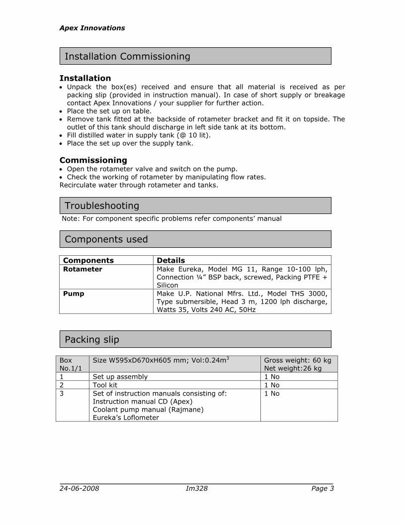
Installation • Unpack the box(es) received and ensure that all material is received as per

packing slip (provided in instruction manual). In case of short supply or breakage contact Apex Innovations / your supplier for further action.

• Place the set up on table. • Remove tank fitted at the backside of rotameter bracket and fit it on topside. The

outlet of this tank should discharge in left side tank at its bottom. • Fill distilled water in supply tank (@ 10 lit). • Place the set up over the supply tank. Commissioning • Open the rotameter valve and switch on the pump. • Check the working of rotameter by manipulating flow rates. Recirculate water through rotameter and tanks.

Note: For component specific problems refer components’ manual

Components Details Rotameter Make Eureka, Model MG 11, Range 10-100 lph,

Connection ¼” BSP back, screwed, Packing PTFE + Silicon

Pump

Make U.P. National Mfrs. Ltd., Model THS 3000, Type submersible, Head 3 m, 1200 lph discharge, Watts 35, Volts 240 AC, 50Hz

Box No.1/1

Size W595xD670xH605 mm; Vol:0.24m3 Gross weight: 60 kg Net weight:26 kg

1 Set up assembly 1 No 2 Tool kit 1 No 3 Set of instruction manuals consisting of:

Instruction manual CD (Apex) Coolant pump manual (Rajmane) Eureka’s Loflometer

1 No

Packing slip

Installation Commissioning

Components used

Troubleshooting

24-06-2008 Im328 Page 4

This product is warranted for a period of 12 months from the date of supply against manufacturing defects. You shall inform us in writing any defect in the system noticed during the warranty period. On receipt of your written notice, Apex at its option either repairs or replaces the product if proved to be defective as stated above. You shall not return any part of the system to us before receiving our confirmation to this effect. The foregoing warranty shall not apply to defects resulting from:

Buyer/ User shall not have subjected the system to unauthorized alterations/ additions/ modifications. Unauthorized use of external software/ interfacing. Unauthorized maintenance by third party not authorized by Apex. Improper site utilities and/or maintenance.

We do not take any responsibility for accidental injuries caused while working with the set up. Apex Innovations Pvt. Ltd. E9/1, MIDC, Kupwad, Sangli-416436 (Maharashtra) India Telefax:0233-2644098, 2644398 Email: san_apexinno@sancharnet.in Web: www.apexinnovations-ind.com

Warranty

24-06-2008 Im328 Page 5

Step response of single capacity system Step function: Mathematically, the step function of magnitude A can be expressed as X (t) = A u (t) where u (t) is a unit step function. It can be graphically represented as

To study the transient response for step function, consider the system consisting of a tank of uniform cross sectional area A1 and outlet flow resistance R such as a valve. qo ,volumetric flow rate through the resistance, is related to head h by a linear relationship qo = h/R -------(1) Writing a transient mass balance around the tank: Mass flow in - Mass flow out = rate of accumulation of mass in the tank. ⟨q (t) - ⟨ qo(t) = d(⟨Ah)/dt q(t) - qo(t) = A1 dh /dt ------(2) Combining equation (1) and (2) to eliminate qo(t) gives the following linear differential equation: q - h/R = A1 dh/dt -------(3) Initially the process is operating at steady state, which means that dh/dt = 0. Therefore equation (3) becomes as qs - hs /R= 0 -----------(4) Where, the subscript s indicates the steady state value of the variable. Subtracting equation (4) from (3) (q - qs) = 1/R ( h - hs) + A1 d(h - hs) / dt ----(5) Defining deviation variable

Theory

24-06-2008 Im328 Page 6

q - qs = Q h - hs = H Equation (5) can be written as Q = 1/R H + A1 dH/dt ---------(6) Taking a transform of equation (6) gives Q(s) = 1/R H(s) + A1s H(s) ----(7) Equation (7) can be rearranged into standard form of first order system as H(s)/Q(s) = R/(τs +1) -----------(8) Where τ = A1R For a step change of magnitude A, we can write Q(t) = A u(t) So Q(s) = A/s From equation (8) we can write H(s) = A/s {R/(τs +1)} -------(9) So by taking Laplace transform of equation (9) we get, H(t) = AR { (1- e -t/τ) } ---------(10)

24-06-2008 Im328 Page 7

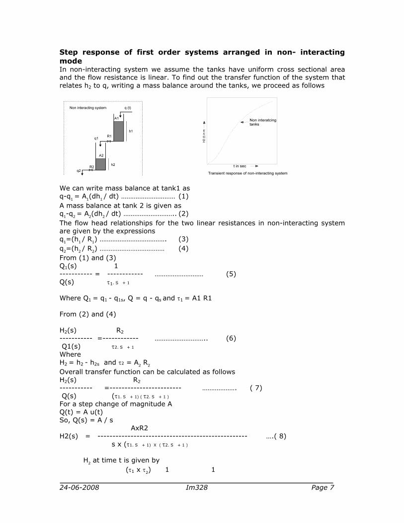
Step response of first order systems arranged in non- interacting mode In non-interacting system we assume the tanks have uniform cross sectional area and the flow resistance is linear. To find out the transfer function of the system that relates h2 to q, writing a mass balance around the tanks, we proceed as follows

We can write mass balance at tank1 as q-q1 = A1(dh1 / dt) ………………………… (1) A mass balance at tank 2 is given as q1-q2 = A2(dh2 / dt) ……………………….. (2) The flow head relationships for the two linear resistances in non-interacting system are given by the expressions q1=(h1 / R1) ………………………………. (3) q2=(h2 / R2) ……………………………… (4) From (1) and (3) Q1(s) 1 ----------- = ------------ ……………………… (5) Q(s) τ1. S + 1 Where Q1 = q1 - q1s, Q = q - qs and τ1 = A1 R1 From (2) and (4) H2(s) R2 ----------- =------------ ……………………….. (6) Q1(s) τ2. S + 1

Where H2 = h2 - h2s and τ2 = A2 R2 Overall transfer function can be calculated as follows H2(s) R2 ----------- =------------------------ ………………. ( 7) Q(s) (τ1. S + 1) ( τ2. S + 1 )

For a step change of magnitude A Q(t) = A u(t) So, Q(s) = A / s

AxR2 H2(s) = -------------------------------------------------- ….( 8) s x (τ1. S + 1) X ( τ2. S + 1 )

H2 at time t is given by

(τ1 x τ2) 1 1

24-06-2008 Im328 Page 8

H2 (t)= A R2 [1 - -------- {--- e-t/ τ1 - ----- e-t/ τ2}] ……………(9) ( τ1- τ2) τ2 τ1

To study impulse response of first order systems arranged in non- interacting mode Mathematically, the impulse function of magnitude A is defined as X(t) = A (t) Where (t) is the unit impulse function. Graphically it can be described as

Overall transfer function of the system as described in previous experiment H2(s) R2 ----------- = ------------------------ ……………… (1) Q(s) (τ1. S + 1) ( τ2. S + 1 ) For a impulse change of magnitude V (volume added to the system) Q(t) = V (t) So, Q (s) = V

VxR2 H2(s) = -------------------------------------------------- … (2) (τ1. S + 1) ( τ2. S + 1) For impulse change H2 at time t is given by e-t/τ1 - e-t/τ2 H2 (t)= V R2 [--------------------------] ………………… (3) ( τ1- τ2)

Considering non-linear resistance at outlet valve of the tank R2 can be calculated as R2 = 2dH2 /dQ Where dH2 is change in level of tank2 and dQ is change of flow from initial to final state. Put the values in equation (3) to find out H (t) Predicted and plot the graph of H (t) Predicted and H (t)Observed Vs time.

24-06-2008 Im328 Page 9

Step response of first order systems arranged in interacting mode Assuming the tanks of uniform cross sectional area and valves with linear flow resistance the transfer function of interacting system can be written as:

H2 (s) R2 ------------------------ = -------------------------------- Q (s) τ1 τ2 s2 +(τ1 + τ2 + A1 R2) s +1

Let 1 1 A1 R2 b = ------- + -------- + -------- τ1 τ2 τ1 τ2

α = (-b/2) + √ [ ( b/2) 2 – ( 1/ τ1 τ2)] β = (-b/2) -√ [ ( b/2) 2 – ( 1/ τ1 τ2)] For a step change of magnitude A

[(1/α) e (αt)] – [(1/β) e (βt)] H2 (t) = AR2 {1 - ---------------------------------}

[1/α - 1/β]

In terms of transient response the interacting system is more sluggish than the non-interacting system.

24-06-2008 Im328 Page 10

Impulse response of first order systems arranged in interacting mode As mentioned in theory part of experiment 3, impulse function is described as X (t)= A (t) Overall transfer function of the system as described in previous experiment

H2(s) R2 -------- = ----------------------------------------- ………(1) Q(s) τ1 τ2 s2 + (τ1 + τ2 + A1 R2) s +1

For a impulse change of magnitude V (volume added to the system) Q(t) = V (t) So, Q (s) = V

V R2 H2(s) = -------------------------------------------------- ---(2)

τ1 τ2 s2 + (τ1 + τ2 + A1 R2) s +1

For impulse change H2 at time t is given by V R2

H2 (t)= ---------------- [e (αt) – e (βt)] -----(3) τ1τ2 (α-β)

(For α, β refer theory part of experiment No. 4) Considering non- linear valve resistance, the resistance at outlet of both tanks can be calculated as R1 = 2 dH1/dQ ------------(4) R2 = 2 dH2/dQ ------------(5)

24-06-2008 Im328 Page 11

1 Step response of single capacity system Procedure • Start up the set up. • A flexible pipe is provided at the rotameter outlet. Insert the pipe in to the cover

of the top Tank 1. Keep the outlet valves (R1 & R2) of the Tank 1 & Tank 2 slightly closed.

• Switch on the pump. Adjust rotameter flow rates in steps of 10 LPH from 50 to 100 LPH and note steady state levels for Tank 1 against each flow rate.

• From the data obtained select a suitable band for experimentation. (Say 90-100 LPH in which we are getting more readings of tank level).

• Adjust the flow rate at lower value of the band selected (say 90 LPH) and allow the level of the Tank 1 to reach the steady state and record the flow and level at steady state.

• Apply the step change by increasing the rotameter flow by @ 10 LPH. • Immediately start recording the level of the Tank 1 at the interval of 15 sec, until

the level reaches at steady state. • Carry out the calculations as mentioned in calculation part and compare the

predicted and observed values of the tank level. • Repeat the experiment by throttling outlet valve (R1) to change resistance. Observations Diameter of tank mm: ID 92 mm Initial flow rate (LPH): Initial steady state tank level (mm): Final flow rate (LPH): Final steady state tank level (mm): (Fill up columns H(t) observed and H(t) predicted after calculations) Sr. No.

Time (sec)

Level (mm)

H(t) observed (mm)

H(t) predicted (mm)

1 0 2 15 3 30 4 --

Calculations H (t) observed = (Level at time t - level at time 0) x 10 –3 m H(t) Predicted = AR { (1- e -t/τ) } Where H (t)Predicted is level predicted at time t in m. A = magnitude of step change = Flow after step input - Initial flow rate in m3/sec. R = Outlet valve resistance in sec/m2 Considering non linear resistance at outlet, it can calculated as R = dH /dQ Where dH is change in level (Final steady state level - Initial steady state level) and dQ is change flow (Final flow rate after step change - Initial flow rate). τ = time constant in sec. =A1 x R Where A1 is area of tank in m2 and R is resistance of outlet

Experiments

24-06-2008 Im328 Page 12

valve in sec/m^2 A1 = Area of tank = ∏/4 (Diameter of tank in m) 2

t = Time in sec from initial steady state. Plot the graph of H(t) Vs time for observed and predicted levels. Sample calculations & results Refer MS Excel program for calculation and graph plotting. Comments Observed response fairly tallies with theoretically calculated response. Deviations observed may be due to following factors: • Non-linearity of valve resistance. • Step change is not instantaneous. • Visual errors in recording observations. • Accuracy of rotameters.

24-06-2008 Im328 Page 13

2 Step response of first order systems arranged in non-interacting mode Procedure • Start up the set up. • A flexible pipe is provided at the rotameter outlet. Insert the pipe in to the cover

of the top Tank 1. Keep the outlet valves (R1 & R2) of both Tank 1 & Tank 2 slightly closed. Ensure that the valve (R3) between Tank 2 and Tank 3 is fully closed.

• Switch on the pump and adjust the flow to @90 LPH. Allow the level of both the tanks (Tank 1 & tank 2) to reach at steady state and record the initial flow and steady state levels of both tanks.

• Apply the step change with increasing the rotameter flow by @ 10 LPH. • Record the level of Tank 2 at the interval of 30 sec, until the level reaches at

steady state. • Record final flow and steady state level of Tank1 • Carry out the calculations as mentioned in calculation part and compare the

predicted and observed values of the tank level. • Repeat the experiment by throttling outlet valve (R1) to change resistance. Observations Diameter of tanks: ID 92mm Initial flow rate (LPH): Initial steady state level of Tank 1 (mm): Initial steady state level of Tank 2 (mm): Final flow rate (LPH): Final steady state level of Tank 1 (mm): Final steady state level of Tank 2 (mm): (Fill up columns H(t) observed and H(t) predicted after calculations) Sr. No. Time

(sec) Level of tank 2 (mm)

H(t) observed (mm)

H(t) predicted (mm)

1 0 2 30 3 60 4 --

Calculations H (t) observed = (Level at time t - level at time 0) x 10 -3 (τ1 x τ2) 1 1 H (t) Predicted = A R2 [1 - -------- { --- e-t/ τ1 - ----- e-t/ τ2}] ------(1) ( τ1- τ2) τ2

τ1

Where H (t)Predicted is level in Tank2 predicted at time t in m. A = magnitude of step change = Flow after step input - Initial flow rate in m3/sec. τ1 = A1 x R1 τ2 = A2 x R2 Where τ1 is time constant of tank1, A1 is area of tank1 and R1 is resistance of outlet valve of tank1. τ2 is time constant of tank2, A2 is area of tank2 and R2 is resistance of outlet valve of tank2 Area of tank 1 = ◊/4 (d1

2) in m2

Area of tank 2 = ◊/4 (d22) in m2

Considering non-linear resistance at outlet valve of both tanks, it can be calculated as

24-06-2008 Im328 Page 14

R1 = dH1 /dQ R2 = dH2 /dQ Where dH1 is change in level of tank1 and dQ is change flow of from initial to final state and dH2 is change in level of tank2 at initial and final state. Put the values in equation (1) to find out H (t) Predicted and plot the graph of H (t) Predicted and H (t)Observed Vs time. Sample calculations & results Refer MS Excel program for calculation and graph plotting. Comments Observed response fairly tallies with theoretically calculated response. Deviations observed may be due to following factors: • Non-linearity of valve resistance. • Step change is not instantaneous. • Visual errors in recording observations. • Accuracy of rotameters.

24-06-2008 Im328 Page 15

3 Impulse response of first order systems arranged in non-interacting mode Procedure • Start up the set up. • A flexible pipe is provided at the rotameter outlet. Insert the pipe in to the cover

of the top tank (T1). Keep the outlet valves (R1 & R2) of both Tank1 & Tank2 slightly closed. Ensure that the valve (R3) between two bottom tanks T2 and T3 is fully closed.

• Switch on the pump and adjust the flow to @90 LPH. Allow the level of both Tank1 and Tank 2, to reach the steady state and record the initial flow and steady state levels of both tanks.

• Apply impulse input by adding 0.5 lit of water in Tank 1. • Record the level of the Tank 2 at the interval of 30 sec, until the level reaches to

steady state. • Record final steady state level of Tank1 • Carry out the calculations as mentioned in calculation part and compare the

predicted and observed values of the tank level. • Repeat the experiment by throttling outlet valve (R1) to change resistance. Observations Diameter of tanks: ID 92mm Initial flow rate (LPH): Initial steady state tank 1 level (mm): Initial steady state tank 2 level (mm): Volume added (lit.): Final steady state tank 1 level (mm): Final steady state tank 2 level (mm): (Fill up columns H(t) observed and H(t) predicted after calculations) Sr. No. Time

(sec) Level of tank 2 (mm)

H(t) observed (mm)

H(t) predicted (mm)

1 0 2 30 3 60 4 --

Calculations H (t) observed = (Level at time t - level at time 0) x 10 -3 e-t/τ1 - e-t/τ2 H2 (t) Predicted = V R2 [--------------------------] ( τ1- τ2)

V = Volume of liquid added as an impulse input (in m3) (For τ1,τ2 and R2 refer values obtained in experiment 2) Put the values in above equation to find out H (t) Predicted and plot the graph of H (t) Predicted and H (t)Observed Vs time. Sample calculations & results Refer MS Excel program for calculation and graph plotting. Comments Observed response fairly tallies with theoretically calculated response. Deviations observed may be due to following factors: • Non-linearity of valve resistance. • Impulse is not instantaneous. • Visual errors in recording observations. • Accuracy of rotameters.

24-06-2008 Im328 Page 16

4 Step response of first order systems arranged in interacting mode Procedure • Start up the set up. • A flexible pipe is provided at the rotameter outlet. Insert the pipe in to the cover

of the Tank 3. Keep the outlet valve (R2) of Tank 2 slightly closed. Ensure that the valve (R3) between Tank 2 and Tank 3 is also slightly closed.

• Switch on the pump and adjust the flow to @90 LPH. Allow the level of both Tank 2 and Tank 3, to reach the steady state and record the initial flow and steady state levels of both tanks.

• Apply the step change with increasing the rotameter flow by @ 10 LPH. • Record the level of the Tank 2 at the interval of 30 sec, until the level reaches at

steady state. • Record final steady state flow and level of Tank 3 • Carry out the calculations as mentioned in calculation part and compare the

predicted and observed values of the tank level. • Repeat the experiment by throttling outlet valve (R1) to change resistance. Observations Diameter of tanks: ID 92mm Initial flow rate (LPH): Initial steady state level of Tank 3 (mm): Initial steady state level of Tank 2 (mm): Final flow rate (LPH): Final steady state level Tank 3 (mm): Final steady state level Tank 2 (mm): (Fill up columns H(t) observed and H(t) predicted after calculations) Sr. No. Time

(sec) Level of tank 2 (mm)

H(t) observed (mm)

H(t) predicted (mm)

1 0 2 30 3 60 4 --

Calculations H (t) Observed = (Level at time t - level at time 0 ) x 10 -3 m

[(1/α) exp (αt)] – [(1/β) exp ( βt)] (H2) t Predicted = AR2 {1 - ---------------------------------------------------} -----(1) [1/α - 1/β]

Where A = magnitude of step change = Flow after step input - Initial flow rate in m3/sec τ1 = A1 x R1 τ2 = A2 x R2 Where τ1 is time constant of tank1, A1 is area of tank1 and R1 is resistance of outlet valve of tank1. τ2 is time constant of tank2, A2 is area of tank2 and R2 is resistance of outlet valve of tank2 Considering non linear resistance at outlet valve of both tanks, it can calculated as R1 = dH1 /dQ and R2 = dH2 /dQ Where dH is change in tank height for change in flow dQ. Calculate values of b, α and β from equations given in theory part. Put the values in equation (1) to find out H (t) Predicted and plot the graph of H (t) Predicted and H (t)Observed Vs time

24-06-2008 Im328 Page 17

Sample calculations & results Refer MS Excel program for calculation and graph plotting. Comments Observed response fairly tallies with theoretically calculated response. Deviations observed may be due to following factors: • Non-linearity of valve resistance. • Step change is not instantaneous. • Visual errors in recording observations. • Accuracy of rotameters.

24-06-2008 Im328 Page 18

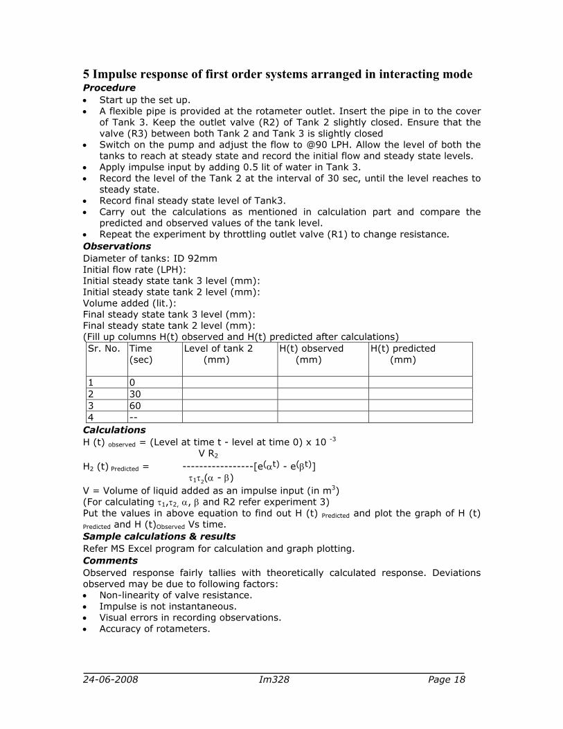
5 Impulse response of first order systems arranged in interacting mode Procedure • Start up the set up. • A flexible pipe is provided at the rotameter outlet. Insert the pipe in to the cover

of Tank 3. Keep the outlet valve (R2) of Tank 2 slightly closed. Ensure that the valve (R3) between both Tank 2 and Tank 3 is slightly closed

• Switch on the pump and adjust the flow to @90 LPH. Allow the level of both the tanks to reach at steady state and record the initial flow and steady state levels.

• Apply impulse input by adding 0.5 lit of water in Tank 3. • Record the level of the Tank 2 at the interval of 30 sec, until the level reaches to

steady state. • Record final steady state level of Tank3. • Carry out the calculations as mentioned in calculation part and compare the

predicted and observed values of the tank level. • Repeat the experiment by throttling outlet valve (R1) to change resistance. Observations Diameter of tanks: ID 92mm Initial flow rate (LPH): Initial steady state tank 3 level (mm): Initial steady state tank 2 level (mm): Volume added (lit.): Final steady state tank 3 level (mm): Final steady state tank 2 level (mm): (Fill up columns H(t) observed and H(t) predicted after calculations) Sr. No.

Time (sec)

Level of tank 2 (mm)

H(t) observed (mm)

H(t) predicted (mm)

1 0 2 30 3 60 4 --

Calculations H (t) observed = (Level at time t - level at time 0) x 10 -3

V R2 H2 (t) Predicted = -----------------[e(αt) - e(βt)]

τ1τ2(α - β)

V = Volume of liquid added as an impulse input (in m3) (For calculating τ1,τ2, α, β and R2 refer experiment 3) Put the values in above equation to find out H (t) Predicted and plot the graph of H (t) Predicted and H (t)Observed Vs time. Sample calculations & results Refer MS Excel program for calculation and graph plotting. Comments Observed response fairly tallies with theoretically calculated response. Deviations observed may be due to following factors: • Non-linearity of valve resistance. • Impulse is not instantaneous. • Visual errors in recording observations. • Accuracy of rotameters.