Embed Size (px)
Citation preview
Two-Sided Markets and Inter-Temporal Trade Clustering: Insights into Trading Motives
Asani Sarkar Senior Economist
Federal Reserve Bank of New York
Robert A. Schwartz Professor of Finance
Zicklin School of Business Baruch College, CUNY
Current Version: March, 2006
We thank Markus Brunnermeier, Michael Goldstein, Joel Hasbrouck, Milt Harris, Terry Hendershott, Murali Jagannathan, Charles Jones, Eugene Kandel, Kenneth Kavajecz, Bruce Lehmann, Albert Menkveld, Maureen O’Hara, Lasse Pederson, Ioanid Rosu, Krystin Ryqvist, Gideon Saar, George Sofianos, Shane Underwood, Jiang Wang, James Weston, Thomasz Wisniewski, and Avner Wolf. We also thank seminar participants at the AFA 2006 meetings, the NBER Market Microstructure conference of October 2005, the Microstructure conference in Norges Bank (Oslo), the 10th Symposium on Finance, Banking and Insurance at the Universität Karlsruhe, Baruch College, Rice University, Rutgers University, SUNY Binghamton, and the Federal Reserve Bank of New York for helpful comments. The views stated here are those of the authors and do not necessarily reflect the views of the Federal Reserve Bank of New York, or the Federal Reserve System.

Abstract
Two-Sided Markets and Inter-Temporal Trade Clustering: Insights into
Trading Motives We show that equity markets are typically two-sided and that trades cluster in certain trading intervals for both NYSE and Nasdaq stocks under a broad range of conditions – news and non-news days, different times of the day, and a spectrum of trade sizes. By “two-sided” we mean that the arrivals of buyer-initiated and seller-initiated trades are positively correlated; by “trade clustering” we mean that trades tend to bunch together in time with greater frequency than would be expected if their arrival was a random process. Controlling for order imbalance, number of trades, news, and other microstructure effects, we find that two-sided clustering is associated with higher volatility but lower trading costs. Our analysis has implications for trading motives, market structure, and the process by which new information is incorporated into market prices.

1
Two-Sided Markets and Inter-Temporal Trade Clustering: Insights into Trading Motives
Market microstructure research has sought to draw inferences about the relative
importance of alternative trading motives from the interaction between price formation and
various indicators of trading activity such as the number and sign of trades, trade size and the
duration between trades. Major efforts include Hasbrouck (1991) who shows that market
makers, by observing trade attributes such as sign and size, can infer information from the trade
sequence. Easley, Kiefer and O’Hara (1996, 1997a, 1997b), using an asymmetric information
model, estimate the arrival rates of informed and uninformed traders using data on the daily
number of buyer-initiated trades, seller-initiated trades, and no-trade outcomes. Dufour and
Engle (2000) find that trades cluster together in time, suggesting that insiders trade quickly to
prevent information leakage.
In this paper, we shed light on the relative importance of the following principle trading
motives: asymmetric information, and differential information and/or beliefs. The asymmetric
information motive has been extensively investigated, while relatively sparse attention has been
given to differential information and/or beliefs. We gain insight into these motives by examining
the joint arrivals of buyer-initiated and seller-initiated trades in intervals ranging from half an
hour down to one minute for a sample of New York Stock Exchange (NYSE) and Nasdaq stocks.
Our methodology involves assessing whether trades are one-sided or two-sided within these
intervals, and whether trades are clustered in time on one or both sides of the market.
By “one-sided” (“two-sided”), we mean that the arrival of more trades triggered by one
side of the market is associated with less (more) trades being triggered by the other side. By
“clustering” we mean that trades bunch together in time more than would be expected if their
arrival was a random process. Thus “two-sided clustering” occurs when intervals with unusually
high numbers of buyer and seller-initiated trades are more prevalent than would be expected
under random trade arrival. Conversely, "one-sided clustering" is indicated by the prevalence of
intervals with unusually large numbers of trades on one side of the market, but not on the other.
Based on a discussion of models of different trading motives (see Section 1), we argue that
trading motivated by asymmetric information leads to one-sided trade clustering, whereas trading
motivated by differential information and/or beliefs results in two-sided trade clustering.
Liquidity needs, a third commonly cited motive for trading, can also result in two-sided markets.
2
We find, for practically every stock in our sample of NYSE and Nasdaq issues, that the
arrivals of buyer-initiated and seller-initiated trades within short time intervals are highly,
positively correlated. In other words, markets generally are two-sided. Moreover, buyer-
initiated and seller-initiated trades tend to cluster together in particular intervals. The results
obtain under a broad range of conditions – news and non-news days, different times of the day,
alternative market structures, and a spectrum of trade sizes. We conclude that trading patterns in
these markets typically exhibit two-sided clustering, consistent with trading motivated by
differential information and/or beliefs.
If informational advantages are short-lived, news-based trading may only be observable
in very small measurement windows. Indeed, using one minute intervals, we find for NYSE
stocks that one-sided trading is evident in the first 15 minutes of days with news, while for
windows longer than a minute and for Nasdaq stocks, two-sided trading remains the norm. This
suggests that trading based on information asymmetries may be a small part of market activity,
consistent with Easley, Engle, O’Hara and Wu (2005) who find that the probability of informed
trading is relatively small (between 8% and 19% for the NYSE stocks in their sample).1
The findings offer important insights into trading motives and the operations of the equity
markets. Previous empirical research has focused on divergent beliefs and/or information as
motives for trading foreign exchange (Lyons, 1995), futures contracts (Daigler and Wiley, 1999),
and treasury securities (Fleming and Remolona, 1999).2 Our findings underscore the
prominence of these same motives for equity trading.3 The clustering suggests that, if some
participants market time the placement of their orders, a substantial, two-sided latent demand to
trade (dark or latent liquidity) may exist at any given time.4 Alternatively, clustering may be
attributed to periodic accelerations of public information arrival.
As we discuss in Section 1, trading based on asymmetric information leads to high
1 Foster and Viswanathan (1994) find, for IBM stock, that much of the information comes in the form of public announcements, and relatively little private information is created in 30 minute intervals. 2 In discussing our paper at the AFA 2006 Meetings, Shane Underwood used data for 1999 for on-the-run 2-Year and 5-Year Treasury Notes to replicate Table 4 in our paper. He found a pattern of two-sided markets similar to what we find for equity markets, reinforcing the association between two-sided markets and the differential interpretations motive. In the context of asset pricing, Anderson, Ghysels and Juergens (2004) show that dispersion of earnings forecasts is a priced factor in traditional factor asset pricing models, and a good predictor of return volatility in out-of-sample tests. 3 Bamber, Barron and Stober (1999) also provide evidence that differential interpretations are an important stimulus for speculative trading in equity markets. 4 Sofinaos (2005) also discusses the significance of latent demand and liquidity.

3
volatility during periods of one-sided trade clustering, trading motivated by differential
information and/or beliefs implies elevated volatility in periods of two-sided trade clustering, and
liquidity trading does not imply any systematic relationship between sidedness and volatility.
We use regression analysis to examine the association between sidedness and price volatility.
Controlling for order imbalance, number of trades, trading costs, time-of-day effects, news
arrival and share price, we find that volatility is highest in intervals with two-sided clustering
after accounting for trading costs. These findings hold for interval lengths ranging from 30
minutes down to one minute; they further highlight the importance of divergent beliefs or
differential information as motives for trading.
Additional investigations confirm the robustness of our results. We assess the effect of
inaccuracies in classifying trade direction by separately examining trades executed inside the
quotes and at mid-quotes.5 Our primary focus is on the post-decimalization period, but we
repeat the analysis for a pre-decimalization period.6 We examine alternative methodologies for
estimating the correlation between buyer-initiated and seller-initiated trades, alternative measures
of news arrival and volatility, and different regression specifications. Consistently, we find that
the equity markets exhibit two-sided clustering.
While the literature has previously focused on order imbalance and the number of trades
to infer trading motives, we show that our sidedness variable contains information not fully
captured by these variables. For example, Easley et al (2005) find that the absolute order
imbalance contains information on informed trade arrivals, while the trade balance (i.e., the
difference between total trades and the absolute order imbalance) reflects uninformed trade
arrivals. We show that markets remain two-sided both in intervals with high or low order
imbalance, and in intervals with many or few trades.7 We suggest that sidedness is informative
even after accounting for order imbalance because it is based on the distributions of buyer- and
seller-initiated trades. Order imbalance, in contrast, is a summary measure of these distributions
5 Trade classification algorithms are less accurate for trades made at the quote (Ellis, Michaely and O’Hara, 2000; Peterson and Sirri, 2003). 6 Decimalization was introduced in January 2001, while our primary sample is from January 2 to May 28, 2003. Trade sizes have decreased in the post decimalization period, and large orders may have been broken up more. 7 We find that markets are more one-sided in intervals with high, compared to low imbalance, and in intervals with few, compared to many, trades. This is consistent with Easley et al (2005) who find that an increase in the absolute order imbalance, relative to total trades, signals a higher arrival rate of informed traders (who are more likely to trade on one side of the market).

4
(i.e. the difference between the numbers of buy- and sell-triggered trades).8
Prior investigations have related the order imbalance to liquidity and volatility. Hall and
Hautsch (2004) find that the instantaneous buy-sell imbalance is a significant predictor of returns
and volatility. Chordia, Roll and Subrahmanyam (2002) show that daily order imbalances are
negatively correlated with liquidity. Even after controlling for order imbalance, we find that our
sidedness variables are highly significant in explaining volatility and trading costs. This further
demonstrates that sidedness is informative even with order imbalance accounted for.
In related papers, Engle and Russell (1994), Engle (1996) and Dufour and Engle (2000)
use the autoregressive conditional duration (ACD) model to estimate inter-trade arrival times. In
contrast to our paper, they do not examine the cross-correlation between the arrivals of buyer-
and seller-initiated trades. Similar to us, Hall and Hautsch (2004) find that buy and sell
intensities evaluated at the time of each transaction are strongly positively auto-correlated and
cross-correlated. However, they examine just three actively-traded stocks on the Australian
Stock Exchange, and their results are robust only for the most active of these stocks. None of
these papers examine the implications of their findings for alternative trading motives.
Our methodology for assessing the sidedness and clustering of markets has an important
advantage relative to time-series based approaches such as those taken by Dufour and Engle
(2000), Hall and Hautsch (2004), and Easley et al (2005). Namely, we are able to aggregate
across relatively large numbers of stocks (both active and less active) and can compare aggregate
trade clustering for various market conditions (e.g. between different times of the day and
between days with and without news events). Because previous methodologies are stock-
specific and computation-intensive, they enable only small numbers of actively traded stocks to
be analyzed;9 thus, they do not allow one to draw conclusions about the broader market (as noted
by Easley et al, 1997a). On the other hand, the disadvantages of our methodology are that we do
not incorporate the dynamics of the buy and sell arrival processes or allow for an interaction
between these dynamics and price formation.10 Our sidedness and clustering variables are best
viewed as an alternative way of characterizing the trade arrival process. In this context, it is
8 For example, sidedness distinguishes between two intervals each with an order imbalance of one, but where the numbers of buyer- and seller-initiated trades could be four and five, or 14 and 15, respectively. 9 Easley et al (1996) aggregate across stocks, but they assume that the information content of each stock is the same in order to reduce the number of parameters to be estimated. 10 For example, in ACD models, the current duration can depend on past durations, and the duration simultaneously affects quote revisions and the correlation between current and past trade direction.

5
reassuring that we do not have results that are inconsistent with those found using the alternative
methodologies.11
Our paper is organized as follows. In Section 1, we discuss alternative models of trading
motives and price formation, and explain how our results relate to predictions from these models.
In Section 2, we describe our data and present descriptive statistics. In Section 3, we examine
the joint distribution of buyer-initiated and seller-initiated trades for NYSE and Nasdaq stocks.
In Sections 4 and 5, we assess the relationships between trade clustering, sidedness and,
respectively, price volatility and trading costs. In section 6, we provide additional analyses to
examine the sensitivity of our results. We conclude in Section 7 by considering the broader
implications of our study. The Appendix contains details of our methodology for estimating the
joint distribution of buyer-initiated and seller-initiated trade arrivals.
1. Trading Motives and Price Formation: Alternative Views and Related Literature
As depicted in Table 1, trading may occur due to asymmetric information (i.e., some
investors have superior information to others); differential information (i.e. some investors have
different information than others) or heterogeneous beliefs (i.e. investors have different
interpretations of news); and/or portfolio rebalancing. The first two columns of Table 1 provide
a summary of the models of trading motives and their implications for sidedness, clustering,
price volatility and trading costs.
When some investors have superior private information (Model 1), a one-sided market is
likely to occur (Wang, 1994; Llorente, Michaely, Saar and Wang 2002). If, for example,
informed traders sell a stock on receiving bad news, its price decreases in the current period.12
When the private information is only partially revealed in the price, insiders are likely to sell
again in the next period.13 Dufour and Engle (2000) suggest that insiders may trade quickly to
11 For example, when we examine the intensity of trade arrivals (independent of whether they are buyer- or seller-initiated), we find, consistent with Engle and Russell (1994) and Engle (1996), that trades cluster in certain intervals and that volatility and trading costs are higher in these periods. 12 We note that one-sided order flow would not obtain in models where price changes follow a martingale (e.g. Kyle, 1985) since if the price change is proportional to order flow (with a fixed constant of proportionality), then order flow must also be a martingale. 13 One might expect that informed traders will generally place market orders. If, instead, most place aggressive limit sell orders on receiving a bad signal, then we may observe a sequence of buyer-initiated trades as market orders from the opposite side hit the limit orders; once again, a one-sided market will result. To the extent that some informed traders use market orders while others place limit orders, the market could be two-sided.

6
prevent information leakage, implying that trades are likely to cluster on one side of the market
following news events.14 Volatility increases in periods of asymmetric information because less-
informed investors demand a larger risk premium to trade against better-informed traders, and so
prices become more responsive to supply shocks (Wang, 1993, 1994).15 Greater volatility and
adverse selection imply that trading costs are also higher with asymmetric information.
Moreover, as asymmetric information leads to one-sided markets, dealers’ inventory imbalances
are likely to be greater, which further leads to higher trading costs.
When investors observe different information signals (Model 2A), each may buy or sell
shares depending on his or her own information signals, implying that informed trading can be
observed on both sides of the market.16 Investors trade many rounds when prices are not fully
revealing, and clustering can occur as investors aggressively acquire speculative positions
immediately after receiving information (He and Wang, 1995). Differential information is
associated with higher volatility because the dispersion magnifies the effect of noisy information
on price changes (Grundy and McNichols, 1990; Shalen, 1993). The effect of differential
information on trading costs is unclear. Uncertainty about the stock value decreases liquidity
(He and Wang, 1995) but, on the other hand, dealers and limit order traders face lower risk from
unbalanced inventory or portfolio positions in two-sided markets, which increases liquidity.
Investors may interpret a public signal differently (Model 2B), with implications for
sidedness, trading costs and volatility that are similar to Model 2A. We expect that trading based
on differential interpretations will lead to two-sided markets. For example, in Kandel and
Pearson (1995), trades occur because agents use different likelihood functions to interpret public
news. Trading can be two-sided if some agents interpret the public signal more optimistically
while others are more pessimistic.17 While models of differential interpretation do not predict
14 Numerical solutions in Foster and Viswanathan (1994) also suggest the possibility of trade clustering in early and late periods after the arrival of information. 15 According to Wang (1993), volatility may even decrease with asymmetric information because uninformed investors have better information about the fundamental value of the stock (due to the information from insider demands and prices) which reduces the uncertainty in future cash flows. However, if there is enough adverse selection in the market, the net effect is for volatility to increase. 16 He and Wang (1995) provide an example of two-sided trading due purely to differential information. In the example (footnote 18 in their paper), half of the investors estimate, based on their information, that the supply shock has increased and buy the stock, while the other half estimate that the supply shock has decreased and sell the stock. 17 Harris and Raviv (1993) develop a model of divergent interpretations where two groups of traders agree whether a signal is positive or negative, but one is more “responsive” to the information. When the cumulative signal is positive (negative), the more responsive (unresponsive) group buys all available shares. As the cumulative signal changes sign, the direction of trades also changes.

7
clustering, if, as trades occur, further trades are executed due to order flow externalities (i.e.
orders attracting orders) then clustering is likely.18 In Kim and Verrecchia (1994), some traders
process public news into private and possibly diverse information about a firm’s prospects; the
information can be interpreted as informed judgments or opinions. They show that, as the
diversity of information increases, there are more information processors, leading to higher
volatility and trading costs. As in Model 2A, the overall relation between diverse opinions and
trading costs is ambiguous because trading costs can be lower in two-sided markets if market
makers are more willing to supply capital owing to lower inventory imbalances.
Finally, investors may trade to rebalance their portfolios (Model 3). For example, if the
returns of traded and non-traded assets are correlated, then uninformed investors may trade to
hedge their non-traded risk (Wang, 1994; Llorente et al 2002). Depending on whether the
correlation is positive or negative, they would buy or sell, leading to two-sided markets. But,
rebalancing trades do not generate more volatility or higher trading costs (He and Wang, 1995).
The consistency of our findings with the various trading motives is indicated in the last
column in Table 1. We find that markets exhibit two-sided clustering and that volatility is
highest during such periods. This is consistent with the predictions of model 2A (differential
information) and model 2B (divergent beliefs).19 Two-sided markets are also predicted by
model 3 (portfolio rebalancing), but our findings of a significant association between sidedness,
volatility and trading costs are inconsistent with model 3’s predictions.
It is difficult to reconcile the findings of two-sided clustering and its association with
high volatility, with Model 1 (asymmetric information). Two-sided clustering may occur if
discretionary liquidity traders and informed traders cluster in the same period (Admati and
Pfleiderer, 1988).20 However, two-sided clustering obtains immediately following news arrival,
when uninformed trades are less likely. Alternatively, if uninformed trades are serially
correlated within a day, then we may not observe one-sided trading sequences following news
arrivals. Yet, we observe two-sided clustering for the largest trades that arrive relatively
infrequently and in less correlated fashion during the day. While the evidence on trading costs is
18 Hendershott and Jones (2005) and Antunovich and Sarkar (2006) provide empirical evidence on order flow externality. 19 Frankel and Froot (1990) also find a positive association between dispersion and price volatility. 20 Easley et al (2005), however, find that an increase in the arrival of informed traders forecasts a decrease in the arrival rates of uninformed traders.
8
consistent with Model 1, it would not be inconsistent with models of differential information or
beliefs once we allow for market maker inventory considerations.
The preponderance of evidence therefore suggests that different interpretations of public
news and/or different private information results in participants trading on opposite sides of the
market. The prevalence of two-sided trading on days with appreciable news release is
particularly striking. While participant responses may not quickly produce new equilibrium
prices, they apparently do move prices rapidly into new trading ranges within which some are
buyers and other are sellers, depending on their individual assessments of the news.
2. Data and Descriptive Statistics
We use time-stamped trade and quote data from the Transactions and Quotes (TAQ)
Database of the NYSE, which records the price, and quantity of trades, as well as dealer quotes.
Our initial data are from January 2 to May 28, 2003, for a matched sample of 41 NYSE stocks
and 41 Nasdaq stocks.21 Later, in section 6, we also examine the pre-decimalization period of
June 2000. To purge the data of potential errors, we delete any trades or quotes with:
1. Zero or missing trade price.
2. Quotes that are missing, negative or unusually small relative to surrounding quotes.
3. Bid (ask) quotes that change from the previous bid (ask) quote by more than $10.
4. The quoted bid-ask spread is negative.
5. The proportional quoted bid-ask spread or effective bid-ask spread is in the upper 0.5
percentile of its distribution by stock and time interval.
6. The quoted bid or ask size is negative.
7. Trade or quote prices that are outside regular trading hours.
)
21 We started with 50 NYSE stocks but had to drop 9 NYSE stocks mostly as they were acquired by or merged with another company. To match based on market value and closing price, we randomly select 41 NYSE stocks that were trading on the last trading day of December 2002, and then select 41 Nasdaq stocks with a market value and closing price that, in combination, were nearest to those of the NYSE stocks on that date. Specifically, for the jth matching variable, let xj be the data for NYSE stock x, and yj be the data for Nasdaq firm y, where j=1 (the market value), or 2 (the closing price). The Euclidean distance between NYSE firm x and Nasdaq firm y is:
(∑=
−=2
1
2),(j
jj yxyxd (1)
We select a matched Nasdaq firm y to minimize d(x,y). Since variables with large variance tend to have more effect on d(x,y) than those with small variance, we standardize the variables before the minimization.
9
These filters eliminated approximately 3% of all recorded prices and quotes. After elimination,
the NYSE data include 4,877,678 trades and the Nasdaq data include 10,860,576 trades.
Initially, we examine trade arrivals in half-hour intervals. Later, in Section 6, we
examine shorter intervals, down to 1 minute in length. The final sample contains 54,226 half-
hour intervals for NYSE stocks and 54,415 half-hour intervals for Nasdaq stocks. We analyze all
trades, and a sample of large trades, which are more likely to be information-based trades of
institutions (e.g. Easley et al, 1997a, find that large trades are twice as informative as small
trades). We define large trades, for a stock, as those that are in the top decile of the dollar value
of trades for that stock in our sample period. This procedure classifies as large trades those with
dollar values that exceed, for the average stock, $32,665 for NYSE and $28,251 for Nasdaq.22
We use the Lee and Ready (1991) algorithm to identify transactions as either buy-
triggered or sell- triggered. If the trade price is closer to the most recent ask (bid) price in the
same stock, it is a buyer (seller) initiated trade. For prices equal to the quote mid-point, trades
that take place on an up tick are buys, and trades that take place on a downtick are sells. The
Lee-Ready (1991) algorithm cannot classify some trades, in particular those executed at the
opening auction of the NYSE, and these are omitted from our sample. In Section 6, we examine
the effects of trade classification errors on our results.
Table 2 gives basic descriptive statistics for our sample. Panel A is for NYSE stocks and
Panel B is for Nasdaq stocks. On January 2 2003, market capitalization and the closing price
averaged $4.7 billion and $21.56 for NYSE stocks and $4.4 billion and $21.35 for Nasdaq
stocks, respectively (values for the two markets are close because the samples are matched). The
table presents measures of volatility and trading costs, as well as the number of buy-triggered
and sell-triggered trades, for different times of the day, and for days with and without news. Our
measure of volatility is HILO, which is the log of the ratio of the maximum to the minimum
price in a period. Our measures of trading costs are PQBAS, the proportional quoted half-spread
and PEBAS, the proportional effective half-spread. Let A (B) be the ask (bid) price. PQBAS is
(A-B)/2M, where M is the quote mid-point. PEBAS is Q(P- M)/M, where P is the trade price,
22 According to Campbell, Ramadorai and Vuolteenaho (2004), trades that are over $30,000 in size are highly likely to be initiated by institutions. Our trade size cutoff is a close match to their number, which provides some assurance that our procedure may distinguish between institutional and retail trades. Institutional trading volume accounts for a large fraction of market volume. Of course, the institutions’ percent of trades is far less than their percent of shares. This implies that the percentage of large trades that is triggered by institutional orders is particularly large.
10
and Q is +1 (-1) for a buy- (sell-) triggered trade, respectively. The reported figures for HILO,
PQBAS, and PEBAS have been multiplied by 100.
The second and third columns of Table 2 show descriptive statistics for news days and
non-news days. Since most news is released during the overnight period, the magnitude of
overnight returns is likely to indicate the impact of news. Accordingly, we define ACLOP as the
absolute value of the excess return (relative to the S&P 500 returns for NYSE stocks and the
Russell 2000 returns for NASDAQ stocks) from the previous day’s close to the current day’s
opening price. To isolate news days, we select the 30 percentile of days where the value of
ACLOP is largest (later, in Section 6, we directly identify days with firm-specific news
events).23 We find that HILO, PQBAS, PEBAS, the number of trades and volume are
significantly higher on news days for both markets, consistent with intuition.
The last five columns of Table 2 show statistics for the first, last and intermediate half-
hours. The first and last half-hours are further divided into 15 minutes intervals; volume and
number of trades are multiplied by two for these intervals for consistency. Volatility, trading
costs and trading activity are all higher in the first half-hour (and the first 15 minutes, in
particular), relative to the middle half-hours, on both markets. Thereafter, trading activity
declines before picking up again 30 minutes before the close, but volatility and trading costs
remain low. In the final 15 minutes, trading activity is highest, and volatility and trading costs
increase, although they remain below the levels of the opening 15 minutes of the day.
The last four rows of the table show statistics for large trades. There are, on average,
only four to five large trades per half-hour interval for NYSE stocks, and only nine to ten large
trades per half-hour interval for Nasdaq stocks.24
3. Order Clustering and the Sidedness of Markets
In this section, we investigate the joint arrivals of buy-triggered and sell-triggered trades.
We examine whether buyer-initiated and seller-initiated trades are correlated in particular
intervals and the extent to which trades cluster in time. Referring to Table 1, if trades are based
23 In Easley et al (2005), the probability that an information event occurs on a particular day is between 0.33 and 0.58 for actively traded stocks. Thus, the 30 percentile cut-off is on the low side of this range, but appears reasonable since we have both active and inactive stocks in our sample. 24 In general, the number of trades is greater in the Nasdaq market than on the NYSE. Historically, the difference has been attributed to the greater prevalence of dealer intermediation in Nasdaq trading.

11
on asymmetric information, we expect the arrivals to be clustered on one-side of the market.
Alternatively, for trading based on differential information or beliefs, we expect that orders
would cluster be on both sides of the market together. Finally, if trading is mainly due to
portfolio rebalancing, markets may be two-sided but need not imply clustering.
Trade clustering may be explained by market participants in general, and by institutional
investors in particular, making strategic timing decisions. Accordingly, we separately study large
trades because they are more likely to be made by institutions that market time their orders.
These trades are also of particular interest because institutions are more apt than retail investors
to be informed, and thus their order flow is more likely to be one-sided than the retail order flow.
But institutional order flow may also be two-sided to the extent that portfolio managers have
diverse motives for trading. For instance, some institutional investors are thought to have
superior information concerning share value (e.g., the value funds), others look only to passively
mimic an index (e.g., the index funds), and yet others seek to exploit short-run trading
opportunities (e.g., the hedge funds). Even funds within the same category (e.g., value funds)
can be on opposite sides of a market if the portfolio managers interpret information differently
(i.e., if they have divergent expectations). Consequently, whether institutional order flow is
predominantly one-sided or two-sided is an empirical issue.
Recognizing that trade clustering could also be an artifact of pooling periods with heavy
trading volume (e.g., the first fifteen minutes of the trading day) with periods when trading is
generally lighter (e.g., in the middle of the day), we examine the pattern separately for the first
and the last 15 minutes of the trading day. We also consider the possibility that trade clustering
is an artifact of pooling periods where little news has occurred with information-rich trading
periods. Thus, we present evidence on trade clustering during the first 15 minute period on news
days. Finally, we address the possible effect of market structure by comparing the patterns of
trade arrivals for NYSE and Nasdaq stocks.
We describe the methodology for determining sidedness and clustering in Section 3A; the
Appendix provides an illustration of the methodology. Results for individual stocks are in
Section 3B, and results for the aggregate of stocks are in Section 3C.

12
A. Methodology
We tabulate the number of buyer-initiated and seller-initiated trades in each interval of
each day, and record the number of intervals for which each specific combination of buyer-
initiated and seller-initiated trades (e.g., two buy triggered trades and three sell triggered trades
in a window) was observed. The results are recorded in a matrix (BSELL matrix from here on).
Our null hypothesis is that buy and the sell arrivals (i.e. the rows and columns of BSELL) are not
associated. To test the hypothesis, we use the Pearson chi-square statistic QP which reflects the
observed minus the expected frequencies, as follows:
( )∑∑
−=
i j ij
ijijP
nQ
εε 2
, (1)
where for row i and column j, is the observed and ijn ijε is the expected frequency. Under the
null hypothesis of independence,nnn ji
ij..=ε where ∑=
jiji nn . is the sum of elements in row i,
is the sum of elements in column j, and ∑=i
ijj nn. ∑∑=i j
ijnn is the overall total. QP has an
asymptotic chi-square distribution under the null with degrees of freedom (R-1)(C-1), where R is
the number of rows and C is the number of columns. For large values of QP, the null hypothesis
is rejected in favor of the alternative hypothesis of dependence between the buy and sell arrivals.
We consolidate the BSELL matrix across stocks to make statements about the aggregate
of buy and sell arrivals over the sample. Since trading activity (and, hence, the size of the
BSELL matrix) differs across stocks, we standardize each BSELL matrix so that stocks with
widely different arrival rates are comparable. To this end, the BSELL matrix is mapped for each
stock into a 3-by-3, High-Medium-Low matrix (HML matrix from now on). We assume that
buy and sell trades follow a random (Poisson) arrival process, with the Poisson parameter λb (for
buys) equal to the mean number of large buy trades, and the Poisson parameter λs (for sells)
equal to the mean number of large sell trades in the sample.25 The mapping rule is based on λb
and λs. Specifically, an interval with nb buy trades is mapped into the:
• LOW BUY cell if nb<=Rounddown(λb-√λb)
25 As will be shown below, the Poisson assumption provides us with a simple, plausible way to transform each BSELL matrix into an HML matrix, and thus to aggregate across stocks.

13
• HIGH BUY cell if nb> Roundup (λb+√λb)
• MEDIUM BUY cell in all other cases.
Intervals with ns sell trades are similarly mapped into LOW, MEDIUM or HIGH SELL
cells based on λs. Note that, since λ is a Poisson parameter, √λ is the standard deviation of the
number of trades for the stock in the sample. Hence, our LOW (HIGH) cutoff represents the
mean minus (plus) the standard deviation of the stock’s trading frequency. The values of λb and
λs used to determine the HIGH, MEDIUM, and LOW cutoffs are specific to each sample (stock
and time-of-day interval). For example, when analyzing a sample of the first 15 minutes of each
day, λb and λs are the mean numbers of buyer-initiated and seller-initiated trades in the first 15
minutes of the trading day.
We report three numbers for each cell of the HML matrix: the observed and unexpected
percent of intervals belonging to the cell, and the percent of QP contributed by the cell. To
obtain these numbers, we aggregate over the relevant cells of the BSELL matrix as determined
by the mapping rule. Specifically, for a given stock and time-of-day interval, let oij be the
observed percent of half-hours, uij be the unexpected percent of half-hours, and Qij be the
Pearson chi-square in cell (i, j) of the BSELL matrix, where
nn
o ijij = (2)
iju = ijijn ε− (3)
( )ij
ijijij
nQ
εε 2−
= , (4)
To obtain the percent of observed and unexpected half-hours in the HML matrix with,
say, LOW BUY and LOW SELL arrivals, we sum oij and uij, respectively, over all cells (i,j) of
the BSELL matrix that are mapped into the LOW,LOW cell of the HML matrix. Similarly, to
obtain the percent of QP contributed by the LOW, LOW cell, we sum Qij over all cells (i,j) of the
BSELL matrix that are mapped into the LOW, LOW cell of the HML matrix, and express this
sum as a percent of QP.
We conduct tests of hypotheses regarding the difference in cell means across different
HML tables (e.g. we compare the mean for a particular cell for all days and the mean for days
with news). Since a stock may not be represented in both tables, the test is implemented for
14
stocks traded in both of the samples being compared. Since the cell counts are positive integers,
we cannot use the ordinary t-statistics. To obtain the standard errors of the cell means, we
assume that the cell counts follow a Poisson distribution, and estimate a Poisson regression of
cell counts on cell and table dummies. Further details on the calculation of these standard errors
are in the Appendix.
B. Individual Stocks Results
In this section, we present evidence that buyer-initiated and seller-initiated trades are
correlated at the individual firm level. To test the null hypothesis that the arrivals of buyer-
initiated and seller-initiated trades in intervals are statistically independent, we compute, for each
stock, the Pearson chi-square statistic.26 The results are shown in Table 3 for the NYSE stocks
(Panel A) and Nasdaq stocks (Panel B). The ticker symbol for each stock is given in column 1;
the chi-square value, the degrees of freedom (DOF), and the associated probability value (P) are
shown in the next three columns. The summary statistics at the bottom of each panel show that
the null hypothesis of independence is rejected at the 1% level of confidence for 39 or more of
the 41 firms in both our NYSE and Nasdaq samples.
Column 5 in the table gives the rank correlation (Corrln) coefficient between buyer-
initiated and seller-initiated trades (i.e. the rows and columns of the BSELL matrix) for each
stock, and column 6 is the P-value for the null hypothesis that the correlation is zero. For all 82
stocks, the null hypothesis of zero correlation is rejected at a high level of significance. For all
stocks, the correlation is positive; it ranges from 0.25 to 0.77 and averages 0.49 (for all trades)
and 0.57 (for large trades) in the NYSE sample, and ranges from 0.25 to 0.94 and averages 0.60
(for all trades) and 0.69 (for large trades) in the Nasdaq sample.
The positive association between buyer and seller-initiated trades indicates that markets
are typically two-sided. Representative patterns of two-sidedness are illustrated in Figure 1 for
three NYSE stocks and three Nasdaq stocks, those with highest, intermediate and lowest trading
frequencies, respectively. The height of each figure shows the percent contribution of each cell
in the HML matrix to the overall chi-square, with “1”, “2” and “3” indicating the LOW,
MEDIUM and HIGH row or column of the HML matrix, respectively. For the most active
26 The Pearson chi-square has previously been used in microstructure studies by, for example, Pasquariello (2001) to examine intra-day patterns in returns and the bid-ask spread in currency markets.

15
NYSE stock, General Motors, and the most active Nasdaq stock, Qualcomm, the HH cell has the
dominant share of the overall chi-square. Figure 1 reflects similar patterns for the less active
stocks. Recall that the HH cell includes intervals with high numbers of buyer and seller-
initiated trades, relative to what would be expected if trade arrivals followed a Poisson process.
Thus, Figure 1 illustrates that the pattern of trade clustering occurs on both the buy and the sell
sides of the market simultaneously, which indicates that the clustering is generally two-sided.
C. Results for the aggregate of stocks
We next examine whether two-sided trade clustering occurs for stocks assessed
collectively. For this purpose, we aggregate the BSELL matrices for individual stocks into one
HML matrix, as described in the methodology section. The results are summarized in Table 4
for the NYSE stocks (Panel A) and NASDAQ stocks (Panel B), respectively. We report results
for the diagonal cells LL (low buyer-initiated and seller-initiated trade arrivals), MM (medium
buyer-initiated and seller-initiated trade arrivals) and HH. Intervals that lie along these three
cells represent two-sided markets since few (many) trades on one side of the market are
associated with few (many) trades on the other side. Two-sided clustering occurs when there are
unusually many intervals in the HH cell indicating that large numbers of buy and sell-triggered
trades bunch together in particular intervals. One-sided clustering occurs when there are
unusually many intervals in the HL (high buyer-initiated and low seller-initiated trade arrivals)
and LH (low buyer-initiated and high seller-initiated trade arrivals) cells indicating large
numbers of trades on one side of the market but few trades on the other. Half-hours that are
neither clearly one-sided nor two-sided are in the (ML, LM) and the (HM, MH) cells (these are
not shown in the table but available from the authors on request).
Each cell contains three statistics, each of which is an average across the stocks: the
observed percentage of half-hours in that cell (in the first row), the unexpected percentage of
half-hours for that cell (in bold, in the second row), and the percentage contribution of the cell
chi-square to the overall chi-square (in the third row). Each panel of Table 4 is divided into four
major rows: all half-hours; the first 15 minutes; the last 15 minutes, and the first 15 minutes on
news days. Results for tests of hypotheses are presented in the last two tables of each panel.
The results for the different panels of Table 4 show a strikingly consistent pattern of two-
sided clustering, even on days with news. Throughout, the incidence of half-hours on the

16
diagonal cells is greater than expected for a random arrival process. Further, the LL and HH
cells contribute the dominant share of the overall Pearson chi-square. For example, in panel A,
for the sample of all trades, the HH cell has 16.42% of the observed number of half-hours, of
which 7.11% are unexpected, and the contribution of this cell to the overall chi-square is
74.61%. The corresponding numbers for the LL cell are 25.51, 7.47 and 8.65, respectively.
In contrast, the number of half-hours with one-sided markets (HL and LH) is less than
expected for a Poisson arrival process. For example, in the HL cell, the three entries are 6.19,
-6.69 and 2.83 for the observed and unexpected percent of half-hours, and the contribution to the
overall chi-square statistic, respectively. More generally, we find that unexpected buy and sell
arrivals are generally negative for all the off-diagonal cells. These findings demonstrate an
unusually large incidence of “HH” and “LL” intervals, and an unusually small incidence of
periods with high trade arrivals on just one side of the market (either on the buy-side or the sell-
side). In other words, trade clustering occurs on both sides of the market simultaneously.
The pattern of two-sided clustering also holds for large trades. This may be attributable
to the strategic timing of trades by institutional investors executing large orders. By extension,
institutional trading in smaller sizes27 and retail day traders may explain the pattern in “all
trades.” Slicing and dicing of large institutional orders results in smaller trades, and can dampen
the trade clustering to the extent that these orders span into different trading intervals.
Two-sided clustering continues to hold for the first and last 15 minutes of the trading day
for both the NYSE stocks and the NASDAQ stocks. Both are periods of heavy volume, and
pooling them with the other intervals could spuriously suggest the presence of trade clustering.
However, the results show that the pattern of two-sided trade clustering holds even in these
heavy volume periods. To illustrate, consider the results for the first 15 minutes for NYSE
stocks for all trade sizes. Two-sidedness is indicated by the positive unexpected percent of
intervals for all diagonal cells and negative unexpected percent of intervals in the cells that
represent one-sided markets. Two-sided clustering is indicated by the large share of the HH cell
in the overall chi-square, almost 37%. This suggests that two-sided clustering is not an artifact
of combining relatively low and high volume periods together.
27 This is consistent with the findings of Campbell, Ramadorai and Vuolteenaho (2004) that institutional trading in small sizes is common.

17
While two-sided markets seem to be the norm qualitatively, the degree of two-sidedness
may differ by time of day. In the bottom two tables of each panel (shown under the heading
“Mean Differences in Observed Percent of Half-Hours”), we report results from tests of
hypotheses for the mean difference in the observed percent of half-hours between different
samples. The first hypothesis relates to the mean difference in the observed percent of half-hours
in the diagonal cells (LL, MM, and HH). The second hypothesis relates to the mean difference
in the observed percent of half-hours in the off-diagonal cells (LH and HL).
The results of hypotheses tests for different times of the day indicate statistically
significant differences in the two-sided pattern. For both NYSE and Nasdaq stocks, the mean
percent of intervals in the diagonal (off-diagonal) cells is generally smaller (larger) for the first
and last 15 minutes compared to the entire day, indicating that markets are less two-sided (more
one-sided) at this time. The result that opening trades are more one-sided and less two-sided is
consistent with the idea that they are more likely to be news-driven compared to other trades. It
is not apparent, however, why closing trades should be less two-sided than other trades.
The final major row in the top Panels of Table 4 shows results for the first 15 minutes of
days with news. The interesting result is that two-sidedness persists on news days much as it
does on all days. For example, considering the sample of large trades, in Panel A (NYSE stocks)
and Panel B (NASDAQ stocks), the HH cell has positive unexpected arrivals of between 5% and
10%, and chi-square shares of almost 50%. In general, considering all and large trades, the
frequency of half-hours in the diagonal cells is greater than expected, and the combined chi-
square share of the diagonal cells is roughly 50%. We conclude that, even on news days, the
incidence of half-hour windows with high numbers of buyer-initiated and seller-initiated trades is
substantially greater than would be expected under a Poisson arrival process.
Turning to the hypotheses tests for news versus non-news days (the last table of each
Panel), we observe that the difference in the mean percent of half-hours is not statistically
significant for either the NYSE or Nasdaq markets, with the exception that, on news days, large
Nasdaq trades are more two-sided and less one-sided. Thus, there is little evidence of more one-
sided trading sequences following news arrivals. A two-sided market following a news event
could be attributed to participants interpreting the import of the new information differently, as
those with relatively optimistic interpretations buy the stock while others sell it.

18
Overall, the evidence of two-sided clustering is similar for the NYSE and Nasdaq
markets for all the samples considered: all trades and large trades, various times of the day, and
days with and without news. Two-sided trade clustering appears to be a general phenomenon
that also transcends structural differences between these two markets.
D. Order imbalance, total trades, and sidedness
In addition to trade clustering and sidedness, cells in the HML matrix also represent
different levels of aggregate trading activity and imbalance in buyer and seller-initiated trades.
For example, the number of trades is lower in the LL cells compared to the HH cells; and,
controlling for total trades, the imbalance in buyer and seller-initiated trades is greater in the off-
diagonal cells than in the diagonal cells. In Easley et al (2005), the absolute imbalance is taken
to reflect informed trade arrivals and balanced trades (i.e. total trades minus the absolute
imbalance) reflect uninformed trade arrivals. Is there information content in sidedness (i.e. cells
in the HML matrix) beyond order imbalance and total trades?
To address this question, we compare the pattern of sidedness for intervals with more
imbalance and less imbalance, relative to the median imbalance. Imbalance is defined as the log
ratio of absolute imbalance to total trades. Table 5 shows the results. In Panel A of the table, we
find that, compared to periods with less imbalance, periods with more imbalance have a greater
unexpected percent of half-hours and larger chi-square shares in the extreme one-sided cells (i.e.
HL and LH) and a lower unexpected percent of half-hours and smaller chi-square shares in the
diagonal cells. The hypotheses test results in Panel B show that, for NYSE (Nasdaq) stocks,
there is about 16% (18%) less observations in the diagonal cells and about 10% (12%) more
observations in the LH and HL cells in high imbalance periods. These results show that periods
with more imbalances are less two-sided and more one-sided, which, consistent with Easley et al
(2005), could imply greater informed trade arrivals. Notably, however, even in periods with high
order imbalance, the pattern of two-sided clustering remains as the unexpected percent of half-
hours is negative in the LH and HL cells and positive in the diagonal cells; further, the chi-square
share of the HH cells exceeds 60%. These results imply that sidedness contains information that
is not fully captured by the buy-sell imbalance.
Table 5 also shows a comparison of buy-sell arrivals for periods of more and less trades,
relative to the median number of trades. The results in Panel B show that periods with more

19
trades are somewhat more two-sided, with about 4% (for NYSE stocks) to 7% (for Nasdaq
stocks) greater observations in the diagonal cells. The results are consistent with greater
uninformed arrivals in periods with more trading. However, even in periods with few trades, the
pattern of two-sided markets obtains as the diagonal cells have a positive unexpected percent of
half-hours along with a combined chi-square share exceeding 50%. Thus, the sidedness variable
is informative even after controlling for total trades and the buy-sell imbalance.
E. Summary: Joint arrivals of buyer-initiated and seller-initiated trades
We find that buyer and seller-initiated trade arrivals are highly positively correlated and
that they cluster together for a wide variety of scenarios (news and non-news days, different
times of the trading day, different trade sizes, and different market structures). Since two-sided
trade clustering also occurs for stocks assessed individually, this finding is not an artifact of
pooling firms that trade a lot with those that trade infrequently. Finally, we find that our measure
of sidedness is informative even after accounting for the buy-sell imbalance and total trades.
4. Sidedness, Trade Clustering and Price Volatility
Engle (1996) finds that a shorter inter-trade time interval is associated with higher
volatility, implying that prices are more volatile in intervals with increased trade clustering.
When we consider aggregate trades (i.e. independent of whether the trades are buyer or seller-
initiated), we show (results not reported, but available from the authors) that, consistent with
Engle, volatility and clustering are correlated. Since the association between volatility and
clustering also depends on investors’ trading motives (see Table 1), in this section we consider
the relationship further, by distinguishing between one-sided and two-sided markets. We first
describe the regression methodology used to assess these relationships, and then present our
findings.
A. Regression methodology
We use regression analysis to examine the relationship between volatility, sidedness and
trade clustering, after controlling for order imbalance, number of trades, news, time-of-day and
other microstructure effects. The log ratio of the highest to the lowest price for an interval
20
(HILO) is our measure of volatility. We regress HILO on dummy variables that reflect the
degree of sidedness and clustering (i.e. cells in the 3x3 High-Medium-Low or HML matrix):
• DUMMY1: equals 1 if the interval falls in the LL cell
• DUMMY2: equals 1 if the interval falls in the MM cell
• DUMMY3: equals 1 if the interval falls in the LH or HL cells
• DUMMY4: equals 1 if the interval falls in the MH or HM cells
• DUMMY5: equals 1 if the interval falls in the HH cell
The omitted cells are the LM and ML cells of the HML matrix. DUMMY1, DUMMY2
and DUMMY5 pertain to cells along the diagonal of the HML matrix that represent two-sided
markets with increasing levels of activity. In particular, DUMMY5 represents intervals where
trades cluster together on both sides of the market. DUMMY3 pertains to the two cells that
represent a one-sided market with clustering, with many trades on one side and few on the other.
DUMMY4 pertains to the two cells that represent an intermediate case between two-sided (i.e.
the HH cells) and one-sided clustering (i.e. the HL and LH cells). Referring to Table 1,
asymmetric information models predict the highest volatility in the HL and LH cells, or that
DUMMY3 will have the largest positive coefficient. Models with differential beliefs or
information predict that volatility will be highest when markets are most two-sided, or that the
coefficient of DUMMY5 will have the highest positive coefficient. Finally, portfolio
rebalancing implies that coefficients on all five dummy variables are insignificant.
The sidedness dummy variables also incorporate variations in aggregate trading activity
and order imbalance. To separate out these effects, we include:
• Log of the number of trades in a half-hour interval
• IMBALANCE: log ratio of the absolute value of order imbalance to the total number of
trades. If the imbalance is zero, we add a small number so that the log is defined.
The descriptive statistics in Table 2 show time-of-day effects on volatility, and that
volatility is higher on days with news. Accordingly, we include the following dummy variables:
• NEWS: equals 1 on days with news.
• [Open, 15 min after open]: equals 1 for the first 15 minutes of the day.
• [15 to 30 min after open]: equals 1 from 15 to 30 minutes after market open.

21
• [30 to 15 min before close]: equals 1 from 30 to 15 minutes before market close.
• [15 min before close]: equals 1 for the last 15 minutes of the day.
Higher volatility and higher trading costs are likely to be correlated.28 Stocks with higher
prices may be more liquid and less volatile. Finally, volatility is known to be persistent. To
account for these effects, we include the following control variables:
• PEBAS: the proportional effective bid-ask half-spread for the interval
• Log of the previous day’s closing price
• Three lags of HILO.29
The reported t-statistics are corrected for autocorrelation and heteroskeasticity with the
Newey-West estimator, and using 14 lags.
B. Effect of sidedness and trade clustering on volatility
We have computed descriptive statistics for volatility for different cells of the HML
matrix. These results (not shown but available from the authors) indicate that, for both the NYSE
and Nasdaq markets, and all trade sizes, the mean and median volatility are generally increasing
as we progress from intervals with few trades (the LL cells) to intervals with two-sided trade
clustering (the HH cells). Intervals in the HH cells have the highest volatility, about 60% greater
than the volatility in intervals with one-sided clustering (the HL and LH cells). For example, for
all NYSE trades, the median HILO (times 100) increases from 0.44 in the LL cell to 1.01 in the
HH cell. Further, the differences in the mean and median volatilities between the different cells
of the HML matrix are statistically significant.
The volatility regression results are given in Table 6, where Panel A is for NYSE stocks,
and Panel B is for Nasdaq stocks. In each panel, results for large and all trades are shown
separately. Results for the five dummy variables for clustering and sidedness are consistent with
the descriptive statistics. For both the NYSE and Nasdaq samples, and for all trade sizes, the
dummy coefficient for the LL cell is negative and significant, whereas the coefficients for
DUMMY2 (the MM cell) and DUMMY5 (the HH cell) are positive and significant. The
DUMMY5 coefficient is the largest in magnitude and the most significant. Thus, all else 28 See, for example, Subrahmanyam (1994). 29 For the first-half hour of the day, we use ACLOP, the absolute excess return from the previous day’s closing to the current day’s opening price, as the first lag of HILO.
22
constant, volatility increases monotonically as we move diagonally from the LL cells to the HH
cells, indicating that volatility is least in two-sided markets with few trades and greatest in two-
sided markets with many trades. Further, the DUMMY3 coefficient (the LH and HL cells) is
positive and significant in three of four cases, but with a magnitude lower than that of
DUMMY5. The DUMMY3 coefficient is also smaller then that of DUMMY2 except for large
NYSE trades. Thus, volatility is high in markets with one-sided clustering, but not as high as in
markets with two-sided clustering. Finally, the DUMMY4 coefficient (the MH and HM cells) is
positive and significant, and with magnitude second only to that of the DUMMY5 coefficient.
The above results obtain even after controlling for total trades and order imbalance. We
find that volatility is significantly and positively correlated with the number of trades in both
exchanges and for all trade sizes. Jones, Kaul and Lipson (1994) and Chan and Fong (2000)
show a similar result using daily data. The coefficient of IMBALANCE does not have a
consistent sign: it is significantly positive (negative) for large (all) NYSE trades, and
insignificantly positive (negative) for large (all) Nasdaq trades. Thus, the effect of imbalance on
volatility appears difficult to interpret.
Others have found that volatility in the opening minutes of trading is high relative to its
value during the rest of the day (see, e.g., Ozenbas, Schwartz, and Wood, 2002). Table 6 shows
that volatility is significantly higher in the first 15 minutes of trading, consistent with opening
volatility being a price discovery phenomenon, as others have suggested. Holding other
variables constant, volatility is significantly lower in the last half-hour of trading (which is
consistent with the descriptive statistics in Table 2).
We find that the coefficient of NEWS is negative and significant. A likely explanation is
that the effect of news arrival is largely captured by increased overnight price volatility, which is
itself accounted for in the regression. Indeed, with lagged values of HILO omitted, the
coefficient of NEWS is positive and significant for both Nasdaq and NYSE stocks.
Regarding the remaining variables, HILO is negatively related to the previous day’s price
(presumably, because stocks with higher prices are generally more liquid and hence less
volatile). Trading costs, as represented by PEBAS, are positively associated with volatility.
Lastly, the three lagged values of HILO are positive and significant, which demonstrates
volatility persistence of up to 1.5 hours in both markets.
23
Overall, the relationships described by the regressions depict an economically coherent
picture. We find that volatility is highest in periods when many buyer-initiated and seller-
initiated trades cluster together, even with order imbalance and total trades accounted for. This
is consistent with trading being motivated by heterogeneous beliefs or information. These results
are harder to reconcile with asymmetric information-based models which predict the highest
volatility in one-sided markets. Finally, the results are inconsistent with trading based on
portfolio rebalancing since we find a significant association between volatility and sidedness.
The adjusted R-squared statistics of around 50% indicate that the independent variables account
for an appreciable proportion of the variation in HILO across our trading intervals.
5. Trade Clustering and Trading Costs
We now turn to the association between trade clustering and trading costs. Engle and
Russell (1994) find evidence of co-movements among duration, volatility, volume, and spread.
When we consider aggregate trades (i.e. independent of whether the trades are buyer or seller-
initiated), we show (results not reported, but available from the authors) that, consistent with
Engle and Russell (1994), trading costs and clustering are correlated. However, sidedness is
likely to be another important determinant of trading costs. Referring to Table 1, asymmetric
information models predict high trading costs when markets are one-sided, whereas the other
models have ambiguous predictions on trading costs. Therefore, we examine the association
between trading costs and the distributions of buyer- and seller-initiated trades.
We repeat the regressions described in the previous section with PEBAS (the
proportional effective half-spread) as the dependent variable.30 There are two differences from
the previous regressions. We include HILO as an explanatory variable since greater volatility
may lead to wider bid-ask spreads by magnifying market maker inventory risks. We also include
three lags of PEBAS to account for autocorrelation in the bid-ask spread.
We examine descriptive statistics for PEBAS for different cells of the HML matrix. The
results (not reported, but available from the authors) show that for both NYSE and Nasdaq
stocks, and for large trade sizes, the mean and median trading costs are highest for one-sided
markets with clustering (the LH, and HL cells). For all trade sizes, PEBAS is generally highest 30 We also have results using PQBAS, the proportional quoted half-spread, as the dependent variable. These results are similar to those using PEBAS and we do not report them (they are available from the authors).
24
in the HH cells, although close in magnitude to its value in the LH and HL cells. In all cases, the
mean and median differences in trading costs between cells are statistically significant.
The trading cost regression results are given in Table 7 for NYSE and Nasdaq stocks, and
for large and all trades. For both markets, and for all trade sizes, trading costs are least in two-
sided markets. For NYSE stocks, the coefficients for DUMMY1, DUMMY2 and DUMMY5
(that represent the LL, MM and HH cells, respectively) are negative and significant (except for
the estimate of DUMMY1 for large trades). For Nasdaq stocks, the DUMMY5 coefficient is
negative and significant, while the coefficients of DUMMY1 and DUMMY2 are negative but not
significant. These results indicate that trading costs are relatively low when markets are two-
sided, even when there are many trades on both sides (recall that volatility is highest in such
cases). In contrast, trading costs are higher in periods with one-sided clustering, as the
DUMMY3 coefficient (representing the HL and LH cells) is mostly positive and significant
(except for large NYSE trades). The coefficient of DUMMY4 is generally not significant.
The effect of sidedness on trading costs persists even after controlling for order
imbalance and trading activity. The regression results show that trading costs are positively and
significantly related to IMBALANCE in all cases, consistent with evidence from daily data.31
We also find that trading costs are significantly and negatively related to total trades in all cases.
Turning to the time-of-day dummies, we observe that trading costs are higher in the first
30 minutes and the last 30 minutes, relative to the rest of the day. While volatility is also higher
in the first 15 minutes, relative to the rest of the day, this result obtains even after controlling for
volatility. The news day dummy coefficient is positive and significant. Trading costs are
negatively related to the prior day’s price level, positively related to contemporaneous volatility,
and are positively autocorrelated.
Overall, the regression results show that – accounting for order imbalance, total trades,
volatility, news, time-of-day and other microstructure effects – trading costs are lower when
markets are two-sided compared to one-sided markets. These findings are consistent with the
predictions of asymmetric-information based models. They are not inconsistent with models
based on heterogeneous beliefs or information which have ambiguous predictions about trading
costs. However, the results are inconsistent with trading based on portfolio rebalancing since we
31 Corwin and Lipson (2000) find that the bid-ask spread increases in response to large order imbalances prior to NYSE trading halts. Chordia et al (2002) find that market liquidity is negatively associated with order imbalances.
25
find a significant association between trading costs and the sidedness dummy variables. The
adjusted R-square is higher than 50% (except for large NYSE trades where it is 26%), indicating
that a large proportion of the variation in PEBAS is explained by our regressions.
Viewed together, the volatility and trading costs results are most consistent with
predictions from models where trading motives are driven by differential beliefs or information.
Thus, the results underscore the importance of such a motive for stock trading.
6. Additional Investigations
So far, we have shown that buyer-initiated and seller-initiated trade arrivals are positively
correlated, indicating that markets are typically two-sided. In this section, we examine the
robustness of our findings. To assess the accuracy of the Lee-Ready (1991) algorithm for
determining the trade direction, we analyze the effects of decimalization and of particular trades
(e.g. those at the mid-quote) that are more likely to be classified inaccurately. We directly
identify days with news events such as earnings releases, instead of the indirect return-based
identification we had used previously. We address the concern that information, and thus one-
sided trading sequences, may be short-lived by considering time intervals as short as one minute.
We explore alternative methodologies for estimating sidedness, and different regression
specifications. We also discuss the possible effect of stale limit orders on our results. Unless
otherwise stated, we do not report any results but they all are available from the authors.
A. The effects of decimalization and of errors in classifying the trade direction
Ellis, Michaely and O’Hara (2000) show, for Nasdaq stocks, and Peterson and Sirri
(2003) find, for NYSE stocks, that the Lee-Ready (1991) algorithm is accurate between 81% and
93% of the time. However, the algorithm is less accurate for trades that are inside the quotes
and, in particular, for trades at the mid-quote; in addition, accuracy is lower for large stocks and
for the post-decimalization period. Accordingly, we repeat our analysis for these types of trades.
In our sample, 10% and 8% of NYSE and Nasdaq trades, respectively, occur at the mid-quote
while 27% and 36% of NYSE and Nasdaq trades, respectively, occur inside quotes but not at the
mid-quote. Since decimalization occurred in January 2001, we choose June 2000 as a pre-
decimalization period. To analyze large and small stocks, we split the sample into the 20 largest
and smallest stocks, based on their market capitalization as of January 3, 2003.
26
The results show that markets are two-sided for all types of trades, with positive
(negative) unexpected arrivals and large (small) chi-square contributions in the diagonal (off-
diagonal) cells of the HML matrix. The hypothesis tests show that, compared to all trades, when
trades are inside the quotes and at the mid-quote, there are more observations on the diagonal
cells and the (HL, LH) cells, and less observations in the intermediate cells. The same is also
true when comparing pre- and post-decimalization trades. Thus, these results do not indicate a
bias towards either more one-sided or more two-sided markets due to trade classification errors,
or due to decimalization. The lack of a bias from decimalization is reassuring since trade sizes
decreased substantially after it was introduced,32 suggesting the possibility that, as more large
orders were broken up, markets became more two-sided after decimalization (assuming large
trades to be more one-sided). However, the results indicate that this is not the case. Indeed, an
examination of large trades in the pre-decimalization period further confirms that two-sided
markets are typical even prior to decimalization. Finally, hypotheses tests comparing the 20
largest and smallest stocks show that the markets for large stocks are moderately more two-sided
than for small stocks, which is consistent with the intuition of market practitioners.
We next investigate whether differences in the buy-sell arrivals for different trade types
(i.e. trades at the mid quote or inside quotes) are reflected in the way sidedness and clustering are
associated with volatility and trading costs. We estimate regressions of HILO and trading costs
on sidedness dummy variables for trades inside the quotes and trades at the mid-quote. The
measure of trading costs is PEBAS for trades at inside quotes and PQBAS for trades at the mid-
quote (since PEBAS is by definition zero for trades at the mid-quote). The results are generally
consistent with earlier findings: HILO is highest in intervals with two-sided clustering (i.e. the
HH cells) and trading costs are highest in one-sided intervals (i.e. the LH and HL cells). The
only exception is that, for NYSE trades at the mid-quote, PQBAS is highest in the MH, HM and
HH cells rather in the LH and HL cells.
Overall, our results for NYSE and Nasdaq stocks are robust to trade classification errors
and to the choice of sample period. In addition, Peterson and Sirri (2003) show that the Lee-
Ready (1991) algorithm works best if no lags are incorporated when matching trades to
prevailing quotes, a procedure we have followed throughout this paper.
32 For example, Chordia, Sarkar and Subrahmanyam (2006) document that, after decimalization, the average daily number of trades for the largest NYSE stocks increased from about 2,400 to almost 4,000.
27
B. Clustering and sidedness on days with corporate news events
Proper identification of news events is essential to finding evidence of informed trade
arrivals and one-sided markets that are more likely to occur following news events. We searched
major publications for news relating to earnings, dividends, mergers and acquisitions, share
repurchases or stock splits, or changes in credit ratings. 39 NYSE stocks and 28 Nasdaq stocks
had news in these categories for our sample period. We find that on days with news, stocks have
significantly higher close-to-open returns or ACLOP, HILO, volume, number of trades, and
PEBAS. These results are virtually identical to those found when using the value of ACLOP to
identify news days (as reported in Table 2).
We estimate the distribution of buyer-initiated and seller-initiated trades for the first 15
minutes of days with news. As previously, we find negative unexpected arrivals in the HL and
LH cells, with a combined chi-square contribution of about 18% for these cells. Further,
unexpected arrivals are generally positive in the diagonal cells except for the MM cell for NYSE
stocks; in addition, the chi-square share of the LL and HH cells add up to about 33% for NYSE
stocks and 50% for Nasdaq stocks. For Nasdaq stocks, there are about 15% more observations
on diagonal cells on news days, indicating that markets are more two-sided at this time. For
NYSE stocks, sidedness is not significantly different for news and non-news days. These results
are similar to what we found previously.
We re-estimate the volatility and trading cost regressions and find that the news dummy
is not significant, whereas in previous regressions it was negative and significant. Most
important, results for the sidedness dummy variables are robust, demonstrating that our results
are not sensitive to alternative identifications of news days.
C. Results using 1-minute windows
Thus far, we have examined sidedness for 15 and 30 minute windows and found no
evidence of one-sided markets. However, if information is generally short-lived, then one-sided
trading sequences may be observed over short measurement windows after news arrival. To
examine this possibility, we repeat our analyses for measurement windows of 10, 5, 3 and 2
minutes and find that markets remain two-sided even on news days. In Table 8, we examine
trade arrivals over 1-minute windows for the first 15 minute of trading days. For all days, Panel
28
A of the table shows that markets are two-sided with negative (positive) unexpected arrivals in
off-diagonal (diagonal) cells. However, for news days, we find evidence of one-sided markets
for NYSE stocks. In particular, unexpected arrivals are positive for LH and HL cells and
negative for LL and MM cells. Note, however, that the combined magnitude of unexpected
arrivals in the LH and HL cells is only about 2%; further, the combined chi-square share of these
cells is about 13%. In addition, for HH cells, unexpected arrivals are positive though small (at
0.39%) and the chi-square share exceeds 46%. Finally, there is no evidence of one-sided trading
in Nasdaq stocks. Panel B of Table 8 shows that for NYSE (Nasdaq) stocks there are about 19%
(5%) greater observations on diagonal cells on all days relative to news days. Thus, there is
evidence of one-sided trading on news days using 1-minute windows, although the evidence is
weak and mostly confined to NYSE stocks.
Panel C of Table 8 shows regressions of trading cost and volatility on sidedness for the
first 15 minutes of the day. The results are similar to those reported for half-hour intervals. In
particular, HILO is highest for two-sided intervals with clustering (i.e. HH cells), and not for
one-sided intervals (i.e. the LH and HL cells), even for NYSE stocks. In unreported results, we
multiplied the sidedness dummies with the NEWS dummy. We found that, for NYSE stocks,
volatility is positively associated with one-sided intervals only for news days, and not for non-
news days. Thus, one-sided trading leads to enhanced volatility, consistent with asymmetric
information-based models. However, volatility continues to be greatest when trade arrivals are
two-sided and clustered.
D. Alternative methodology for estimating sidedness
Our evidence for two-sided markets is based on the HML matrix, where the low, medium
and high cutoffs are derived (assuming Poisson order arrivals) using the square root of the mean
number of buyer and seller-initiated trades for each stock. As an alternative, we now use the
actual standard deviation of trade arrivals. Specifically, we calculate the z-score for a stock in an
interval as the number of buyer or seller-initiated trades minus the sample mean, and divided by
the sample standard deviation.33 We then compute the correlation between the z-scores for
buyer and seller-initiated trades. A large and positive correlation indicates two-sided markets.
33 We thank Eugene Kandel for suggesting this approach to us. The results are similar if we subtract the z-score for the “market,” defined as the average z-score for all stocks in the interval.

29
We find that, for all intervals, the average correlation is 0.49 for NYSE stocks and 0.60 for
Nasdaq stocks. For the first 15 minutes of a day, the correlation drops to 0.35 for NYSE stocks
and to 0.51 for Nasdaq stocks. For the first 15 minutes of news days, the correlation is 0.32 for
NYSE stocks and 0.54 for Nasdaq stock. These results are consistent with two-sided clustering,
and with relatively more one-sided trading during the first 15 minutes of the trading day. As
previously, news arrivals do not make a substantial difference to sidedness.
E. Alternative regression specifications and volatility definitions
We estimate a number of alternative specifications for the regressions, and use an
alternative definition of volatility, and find the results are similar to those reported earlier. In
particular, it remains true that volatility is highest in the HH cells, while trading costs are highest
in the LH and HL cells for both NYSE and Nasdaq stocks.
To further control for stock-specific factors, we estimate a regression with fixed effects
for each stock.34 Next, to account for the fact that HILO and PEBAS are always between 0 and
1, we estimate an accelerated failure time model assuming that the data are censored on the left
at zero and on the right at one and that the failure time follows a logistic distribution.35
For the volatility regression, we perform two more checks. We examine whether the
strong association of volatility and two-sided clustering is due to intervals with an unusually
large number of trades.36 Next, we repeat our analysis with two alterative definitions of
volatility: the log ratio of the maximum to the minimum mid-quote; and the sum of 1-minute
squared returns in an interval. These alternative definitions address the concern that, with our
original definition (based on the trade price), volatility may also include the bid-ask bounce.
34 When stock-specific fixed effects are introduced, one result different from before is that in the volatility regression the DUMMY3 coefficient is either not significant or is negative and significant, indicating that volatility is relatively low in one-sided markets with clustering. 35 The classic Tobit model is a special case of the estimated model. In the Tobit model, the failure time is normally distributed and the data is usually censored at the left. The estimates from the logistic distribution are robust since they have bounded influence functions (an influence function measures the difference in standard deviation units between estimates with and without an individual observation). 36 Specifically, we include the square of the (log of) trades in the regression. The non-linear term is positive and significant, and reduces the significance of the log trade term, but remaining terms are unaffected.
30
F. Effect of stale limit orders
The arrival of good news may prompt an influx of market buy orders that hit standing
limit orders before they can be withdrawn, causing a clustering of buyer-initiated trades.37
Similarly, bad news may cause a clustering of seller-initiated trades. Note, however, that our
results show trade clustering on both sides of the market. Thus, for stale limit orders to cause
two-sided markets, good news must typically follow bad news, or vice versa, within our
measurement interval. Moreover, we find that two-sided markets endure even with a short
measurement window of 1-minute and in the most active intervals (see Table 5). Accordingly, it
is appears unlikely that our results are due primarily to the presence of stale limit orders.
7. Conclusion
We have sought to gain further insight into alternative motives for trading (superior
information, differential information and/or beliefs, and liquidity reasons), by examining the
pattern of buyer-initiated and seller-initiated trade arrivals in the two major U.S. market centers,
the NYSE and Nasdaq. Of primary interest is the systematic tendency for these markets to be
two-sided in relatively brief intervals (from 30 minutes to 1 minute) and for trades to cluster
together in time within a day. For both markets, we have observed that arrivals of buyer- and
seller-initiated trades are highly positively correlated. Further, buyer and seller-initiated trades
tend to bunch together in particular intervals with greater frequency than would be expected
under random trade arrival.
We have considered the association of the two-sided trade bursts with price volatility.
Controlling for order imbalance, number of trades, news arrival, time-of-day effects and share
price, we observe that (in comparison with one-sided markets) two-sided trade bursts are
associated with higher volatility.
Our sidedness variable contains information that is not fully captured by order imbalance
and total trades. We find that markets are two-sided even in periods of relatively high
imbalance. Further, our sidedness variables are highly significant in explaining volatility and
trading costs with imbalance and total trades controlled for. We suggest that sidedness is
informative because it depends more broadly on the distributions of buyer-initiated and seller-
37 We thank Joel Hasbrouck for suggesting this possibility that stale limit orders may cause clustering.

31
initiated trades, whereas order imbalance is a summary measure of these distributions.
Our findings are robust. Two-sided markets are the norm for the array of conditions that
we have considered: marketplace, trade size, time of day, and information environment.
Particularly striking is the extent to which two-sidedness continues to prevail on days with news
release. Apparently, markets are efficient in that prices move rapidly into new trading ranges
within which some participants are looking to buy, and others are seeking to sell shares. Our
results are robust to errors in classifying trade direction, to the sample period (i.e. pre- versus
post-decimalization), and to alternative methodologies for estimating sidedness.
We find evidence of one-sided trading sequences that could be motivated by asymmetric
information in the first 15-minutes of news days when we examine windows of 1-minute
duration. Aside from this, the wide-spread prevalence of two-sided clustering and its
relationship with volatility and trading costs strongly suggests that two-sided trade clustering is
not necessarily attributable to the arrival of new fundamental information per se but instead may
arise from participants having different information and/or divergent beliefs.
Trade clustering suggests that some orders at least are portable in time. That is, orders
may be kept in traders’ pockets until something occurs in the marketplace that leads participants
on both sides of the market to step forward and trade. Whatever seeds or animates the process,
trading appears to gain strength as the latent demands of both buyers and sellers are turned into
active orders and realized trades. As this happens, the time duration between trades decreases
and a trade burst occurs.
Two-sided clustering indicates that natural buyers and natural sellers (the investors) are
generally present in the market at the same time and, consequently, that they should, in principle,
be able to supply liquidity to each other. However, the existence of latent (or dark) liquidity
suggests that intermediaries may be needed in the marketplace to animate trading.38 Additional
market structure (such as that provided by various alternative trading systems) may also be
needed. In light of this, a further examination of trade clustering and the magnitude of latent
liquidity would be desirable.
38 The term “animation” applies specifically to an intermediary contacting potential buyers and sellers and/or by actually triggering trades themselves. More generally, exchange floor traders and market makers are widely recognized as being market facilitators to the extent that they actively bring buyers and sellers together. In part, they might do so by stimulating book building and by triggering trades.

32
Circumstantial evidence suggests that latent liquidity may be consequential. In the
current environment, it is well known that large institutional traders typically slice and dice their
big orders for execution over extended periods of time (up to a day or more).39 This reality is
reflected by the fact that average trade size on the NYSE has declined from a peak of 2303
shares in 1988 to 343 shares in June 2005. Concurrently, block-trading volume (trades of 10,000
shares or more) on the NYSE has dropped sharply from 51.1% of reported volume in 1988 to
27.9% in June 2005 (www.nysedata.com/factbook). New trading facilities such as Liquidnet and
Pipeline have been designed with explicit reference to the need for better quantity discovery.
Moreover, evidence suggests that institutional participants’ demand for immediacy is largely
attributable to the dynamics of the marketplace (which include, e.g., front running), and that
portfolio managers commonly give their traders a day or more to work their orders.40
The prevalence of two-sided trade clustering and its association with volatility and
trading costs underscore the importance of differential information and/or beliefs as a motive for
trading. We leave for future research a more complete analysis of what might spark the bouts of
intensified trading.
39 Traders bring their orders carefully to the market for two reasons. First, they are concerned about market impact costs. Second, being subjected to trader performance evaluations, they are reluctant to trade at “undesirable” prices (i.e., buy above or sell below the volume weighted average price for a trading session). Both considerations lead participants to bring their orders to the market in smaller pieces that are executed over an extended period of time. 40 See Schwartz and Steil (2002) for discussion and further references.

33
References
1. Admati, A.R. and P. Pfleiderer, 1988, A Theory of Intraday Patterns: Volume and Price Variability, Review of Financial Studies, 1, 3-40.
2. Anderson, E. W., E. Ghysels and J. L. Juergens, 2004, Do Heterogeneous Beliefs Matter for Asset Pricing? Working Paper, University of North Carolina at Chapel Hill.
3. Antunovich, P. and A. Sarkar, 2006, Fifteen Minutes of Fame? The Market Impact of
Internet Stock Picks, forthcoming, Journal of Business.
4. Bamber, L. D., O. E. Barron and T. L. Stober, 1999, Differential Interpretations and Trading Volume, Journal of Financial and Quantitative Analysis, 3, 369-386.
5. Benston, G., and R. Hagerman, 1974, Determinants of Bid-Asked Spreads in the Over-The-Counter Market, Journal of Financial Economics, 1, 353-364.
6. Campbell, J. Y., Ramadorai, T. and T. Vuolteenaho, 2004, Caught on Tape: Predicting
Institutional Ownership with Order Flow, Working Paper, Harvard University.
7. Chan, K. and W. Fong, 2000, Trade Size, Order Imbalance, and the Volatility-Volume Relation, Journal of Financial Economics, 57, 247-273.
8. Chordia, T., R. Roll and A. Subrahmanyam, 2002, Order Imbalance, Liquidity and
Market Returns, Journal of Financial Economics, 65, 111-130.
9. Chordia, T., A. Sarkar and A. Subrahmanyam, 2006, Liquidity Dynamics and Cross Autocorrelations, Working Paper, Anderson School of Management, UCLA.
10. Corwin, S. and M. L. Lipson, 2000, Order Flow and Liquidity Around NYSE Trading
Halts, Journal of Finance, 55, 1771-1801.
11. Daigler, R. T. and M. K. Wiley, 1999, The Impact of Trader Type on the Futures Volatility- Volume Relation, Journal of Finance, 54, 2297 – 2316.
12. Dufour, A. and R. F. Engle, 2000, Time and the Price Impact of a Trade, Journal of
Finance, 55, 2467-2498.
13. Easley, D., N. M. Kiefer and M. O’Hara, 1996, Cream Skimming or Profit Sharing, Journal of Finance, 51, 811-833.
14. Easley, D., N. M. Kiefer and M. O’Hara, 1997a, The Information Content of the Trading Process, Journal of Empirical Finance, 4, 159-186.
15. Easley, D., N. M. Kiefer and M. O’Hara, 1997b, One Day in the Life of a Very Common Stock, Review of Financial Studies, 10, 805-835.

34
16. Easley, D., R. F. Engle, M. O’Hara and L. Wu, 2005, Time-Varying Arrival Rates of Informed and Uninformed Trades, Working Paper.
17. Ellis, K., R. Michaely and M. O’Hara, 2000, The Accuracy of Trade Classification Rules:
Evidence from Nasdaq, Journal of Financial and Quantitative Analysis, 35, 4, 529-551.
18. Engle, R. F., 1996, The Econometrics of Ultra-High Frequency Data, Discussion Paper 96-15, Department of Economics, University of California, San Diego.
19. Engle, R. F. and J. R. Russell, 1994, Forecasting Transaction Rates: The Autoregresive
Conditional Duration Model, NBER Working paper No. 4966.
20. Fleming, M. and E. M. Remolona, 1999, Price Formation and Liquidity in the U.S. Treasury Market: The Response to Public Information, Journal of Finance, 54, 1901-1915.
21. Foster, F. D. and S. Viswanathan, 1994, Strategic Trading with Asymmetrically Informed Traders and Long-Lived Information, Journal of Financial and Quantitative Analysis, 29, 4, 499-518.
22. Frankel, J. F. and K. Froot, 1990, Chartists, Fundamentalists and Trading in the Foreign
Exchange Market, American Economic Review, 80, 181-185.
23. Grundy, B. D. and M. McNichols, 1990, Trade and the Revelation of Information Through Prices and Direct Disclosure, Review of Financial Studies, 2, 495-526.
24. Hall, A. D. and N. Hautsch, 2004, A Continuous Time Measurement of the Buy-Sell Pressure in a Limit Order Book Market, Working Paper, University of Copenhagen.
25. Harris, M. and A. Raviv, 1993, Differences of Opinion Make a Horse Race, Review of Financial Studies, 6, 473-506.
26. Hasbrouck, J., 1991, Measuring the Information Content of Stock Trades, Journal of
Finance, 46, 179-207.
27. He, Hua and Jiang Wang, 1995, Differential Information and Dynamic Behavior of Stock Trading Volume; Review of Financial Studies; 8, 919-972.
28. Hendershott, T. and C. M. Jones, 2005, Island Goes Dark: Transparency, Fragmentation, and Regulation, Review of Financial Studies, 18, 743-793.
29. Jones, Charles M., G. Kaul, and M. L. Lipson, 1994, Transactions, Volume and Volatility; Review of Financial Studies, 7, 631-651.
30. Kandel, E. and N. D. Pearson, 1995, Differential Interpretation of Public Signals and
Trade in Speculative Markets, Journal of Political Economy, 103, 831-872.

35
31. Kim, O. and R. E. Verrecchia, 1994, Liquidity and Volume Around Earnings
Announcements, Journal of Accounting and Economics, 17, 41-67.
32. Kyle, A.S., 1985, Continuous Auctions and Insider Trading, Econometrica, 53, 1315-1335.
33. Lee, C. and M. Ready, 1991, Inferring Trade Directions from Intraday Data, Journal of
Finance, 46, 733-746.
34. Llorente, G., R. Michaely, G. Saar and J. Wang, 2002, Dynamic Volume-Return Relation of Individual Stocks, Review of Financial Studies, 4, 1005-1047.
35. Lyons, Richard K., 1995, Tests of Microstructural Hypotheses in the Foreign Exchange
Market, Journal of Financial Economics, 39, 321-351.
36. Ozenbas, D, R. Schwartz and R. Wood, 2002, Volatility in U.S. and European Equity Markets: An Assessment of Market Quality, International Finance, 5, 437-461.
37. Pasquariello, P., 2001, The Microstructure of Currency Markets: An Empirical Model of
Intra-day Return and Bid-Ask Spread Behavior; Working Paper, University of Michigan.
38. Peterson. M. and E. Sirri, 2003, Evaluation of the Biases in Execution Cost Estimation Using Trade and Quote Data, Journal of Financial Markets, 6, 259-280.
39. Schwartz, R. and B. Steil, 2002, Controlling Institutional Trading Costs: We Have Met the
Enemy, and it is Us, The Journal of Portfolio Management, 28, 39-49.
40. Shalen, C. T., 1993, Volume, Volatility and the Dispersion of Beliefs, Review of Financial Studies, 6, 405-434.
41. Sofianos, G., 2005, The Changing Nature of Intermediation, Working Paper, The
Goldman Sachs Group, Inc.
42. Subrahmanyam, A., 1994, Circuit breakers and market volatility: A theoretical perspective, Journal of Finance, 49, 237-254.
43. Wang, J., 1993, A Model of Intertemporal Asset Prices Under Asymmetric Information,
Review of Financial Studies, 60, 249-282.
44. Wang, J., 1994, A Model of Competitive Stock Market Trading, Journal of Political Economy, 102, 127-168.

36
Appendix: Methodology for Hypotheses Tests
We provide an illustration of the methodology for estimating the joint distribution of
buyer-initiated and seller-initiated trades, and then discuss details of the Poisson regression used
to calculate standard errors for hypothesis testing in Table 4.
A. Estimating joint distribution of buyer and seller-initiated trade arrivals: An Illustration
To illustrate, suppose we have a stock that averages 4 large buy trades and 3 large sell
trades per half-hour. Further, suppose that there is a maximum of 8 large buys and 6 large sell
trades in the half-hour intervals in our sample. We first construct a 9-by-7 buy-sell matrix (that
includes additional cells for no large buyer-initiated and for no large seller-initiated trades).
Each cell, ranging from (0,0) to (8,6), gives the number of half-hours with the specific buy-sell
combination for that cell. The Pearson chi-square QP is then computed as described in (1) of the
text. The 9-by-7 matrix is mapped into a 3-by-3 matrix as follows:
• Half-hours with 2 large buy trades (the mean of 4 minus the standard deviation of 2) or less
are mapped into a LOW BUY cell; and half-hours with 1 (the mean of 3 minus the square
root of 3 rounded down) or zero large sell trades are mapped into a LOW SELL cell.
• Half-hours with 6 or more large buy trades are mapped into a HIGH BUY cell; and half-
hours with 5 or more large sell trades are mapped into a HIGH SELL cell.
• Half-hours with more than 2 but less than 6 large buy trades are mapped into a MEDIUM
BUY cell; and half-hours with more than 1 but less than 5 large sell trades are mapped into a
MEDIUM SELL cell.
The arrival frequency in the LOW, LOW cell is obtained by summing oij over i=0,1,2 and j=0,1.
The contribution of the LOW, LOW cell to QP is obtained by summing Qij over i=0,1,2 and
j=0,1, and expressing the sum as a percent of QP. Numbers for the other cells are obtained in
similar fashion.
B. Tests of hypotheses
We conduct tests of hypotheses regarding the difference in cell means across different
HML tables (e.g. comparing the mean for cell HH between the table for NYSE stocks and the
table for Nasdaq stocks). To obtain the standard errors of the cell means, we assume that the cell
counts for different stocks and tables follow a Poisson distribution.

37
Denote ntijs as the cell count for row i and column j in table t for stock s. We compare two
tables at a time, so t=1,2. Let nts denote the sum of cell counts for table t and stock s. Further, let
Iijt denote an indicator variable that equals 1 for row i, column j and table t, and is zero otherwise.
Then, we estimate a Poisson regression model as follows:
tjit i j
tjitjitstijs uInn +++= ∑∑∑= = =
2
1
3
1
3
110 )log()log( βββ (A1)
β1 is assumed to be 1, so that log(nst) is interpreted as a so-called offset variable; it
normalizes the fitted cell means to a percent of the total cell count for the stock and the table. utji
is the error term. The regression (A1) is estimated by maximizing the log-likelihood function
L=∑ with respect to the regression parameters. l=
738
1iil i is the log-likelihood for the i-th observation,
and the total number of observations is 738 (equal to the number of stocks (41) times the number
of cells (9) times the number of tables (2)). For the Poisson distribution, li has the form:
iiii nl μμ −= )log( (A2)
L is maximized using a ridge-stabilized Newton-Raphson algorithm (details available from
the authors). In all cases, the algorithm converged.
We estimate regression (A1) to obtain the cell means and standard errors for each table,
which are then used to calculate t-statistics for testing hypotheses about mean differences in the
usual way. For example, the estimated percent means for cell HH in tables 1 and 2 are given by:
1331330133ˆˆˆ Aββμ +=
2332330233ˆˆˆ Aββμ += (A3)
Suppose that the corresponding standard errors are estimated as and . Then, to test
whether the mean for cell HH in table 1 is different from that in table 2, the t-statistic is:
133ˆes 233ˆes
( ) ( )22332
133
233133
ˆˆ
ˆˆ
esest
+
−=
μμ (A4)
The degree of freedom for the t-statistic is 736, since the total number of observations is 738
(equal to the number of stocks (41) times the number of cells (9) times the number of tables (2)).
We also compare the sum of cell means (e.g. the mean for cell LH plus the mean of cell HL)
across tables. In this case, to obtain the standard errors, we assume for simplicity that the
variance of the sum of means is equal to the sum of the variances of the means.

38
Table 1: Models, Predictions, and Findings The table presents three models of investor trading motives, each model's implications for sidedness, clustering, price volatility and trading costs, and whether the findings of this paper are consistent with the predictions. The trading motives are: asymmetric information (Model 1), different information and/or different beliefs (Model 2), and portfolio rebalancing (Model 3). N.A. indicates that a finding is neither consistent nor inconsistent because the prediction it is matched with is ambiguous.
Model Implications Consistent With Our Findings? 1. Some investors have superior information about asset value (Wang , 1993, 1994; Llorente, Michaely, Saar and Wang, 2002)
• One-sided markets • Trade clustering on one side of the
market • Higher volatility when markets are
one-sided • Higher trading cost when markets
are one-sided
• No
• No • No • Yes
2. Investors have different private information signals (Grundy and McNichols, 1989; Shalen, 1993; He and Wang, 1995) and/or different beliefs (Kim and Verrecchia, 1994; Kandel and Pearson, 1995)
• Two-sided markets • Trade clustering on both sides of
the market • Higher volatility when markets are
two-sided • Ambiguous effect on trading costs
• Yes • Yes • Yes • N.A.
3. Investors trade to rebalance their portfolios (Wang , 1994; He and Wang, 1995; Llorente, Michaely, Saar and Wang, 2002)
• Two-sided markets • No implication for clustering • No relation between sidedness and
volatility • No relation between sidedness and
trading costs
• Yes • No • No • No
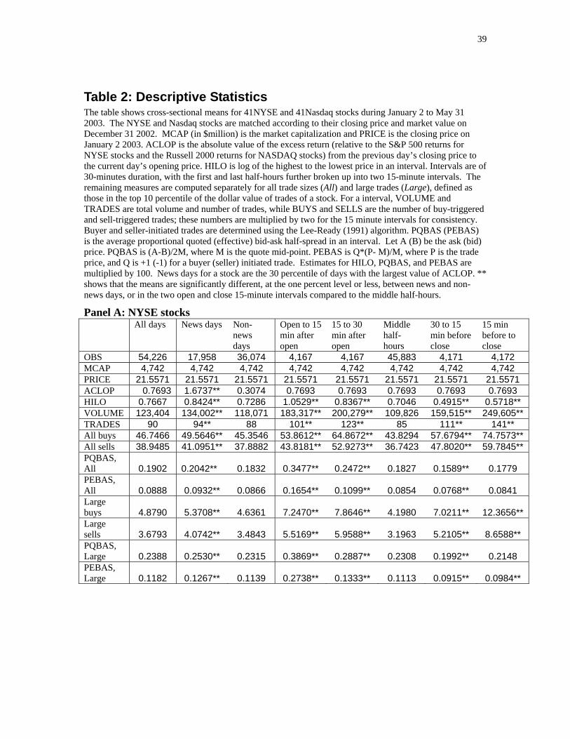
39
Table 2: Descriptive Statistics The table shows cross-sectional means for 41NYSE and 41Nasdaq stocks during January 2 to May 31 2003. The NYSE and Nasdaq stocks are matched according to their closing price and market value on December 31 2002. MCAP (in $million) is the market capitalization and PRICE is the closing price on January 2 2003. ACLOP is the absolute value of the excess return (relative to the S&P 500 returns for NYSE stocks and the Russell 2000 returns for NASDAQ stocks) from the previous day’s closing price to the current day’s opening price. HILO is log of the highest to the lowest price in an interval. Intervals are of 30-minutes duration, with the first and last half-hours further broken up into two 15-minute intervals. The remaining measures are computed separately for all trade sizes (All) and large trades (Large), defined as those in the top 10 percentile of the dollar value of trades of a stock. For a interval, VOLUME and TRADES are total volume and number of trades, while BUYS and SELLS are the number of buy-triggered and sell-triggered trades; these numbers are multiplied by two for the 15 minute intervals for consistency. Buyer and seller-initiated trades are determined using the Lee-Ready (1991) algorithm. PQBAS (PEBAS) is the average proportional quoted (effective) bid-ask half-spread in an interval. Let A (B) be the ask (bid) price. PQBAS is (A-B)/2M, where M is the quote mid-point. PEBAS is Q*(P- M)/M, where P is the trade price, and Q is +1 (-1) for a buyer (seller) initiated trade. Estimates for HILO, PQBAS, and PEBAS are multiplied by 100. News days for a stock are the 30 percentile of days with the largest value of ACLOP. ** shows that the means are significantly different, at the one percent level or less, between news and non-news days, or in the two open and close 15-minute intervals compared to the middle half-hours.
Panel A: NYSE stocks All days News days Non-
news days
Open to 15 min after open
15 to 30 min after open
Middle half-hours
30 to 15 min before close
15 min before to close
OBS 54,226 17,958 36,074 4,167 4,167 45,883 4,171 4,172 MCAP 4,742 4,742 4,742 4,742 4,742 4,742 4,742 4,742 PRICE 21.5571 21.5571 21.5571 21.5571 21.5571 21.5571 21.5571 21.5571 ACLOP 0.7693 1.6737** 0.3074 0.7693 0.7693 0.7693 0.7693 0.7693 HILO 0.7667 0.8424** 0.7286 1.0529** 0.8367** 0.7046 0.4915** 0.5718** VOLUME 123,404 134,002** 118,071 183,317** 200,279** 109,826 159,515** 249,605** TRADES 90 94** 88 101** 123** 85 111** 141** All buys 46.7466 49.5646** 45.3546 53.8612** 64.8672** 43.8294 57.6794** 74.7573** All sells 38.9485 41.0951** 37.8882 43.8181** 52.9273** 36.7423 47.8020** 59.7845** PQBAS, All
0.1902 0.2042** 0.1832
0.3477**
0.2472**
0.1827
0.1589**
0.1779
PEBAS, All
0.0888 0.0932** 0.0866
0.1654**
0.1099**
0.0854
0.0768**
0.0841
Large buys
4.8790 5.3708** 4.6361
7.2470**
7.8646**
4.1980
7.0211**
12.3656**
Large sells
3.6793 4.0742** 3.4843
5.5169**
5.9588**
3.1963
5.2105**
8.6588**
PQBAS, Large
0.2388 0.2530** 0.2315
0.3869**
0.2887**
0.2308
0.1992**
0.2148
PEBAS, Large
0.1182 0.1267** 0.1139
0.2738**
0.1333**
0.1113
0.0915**
0.0984**
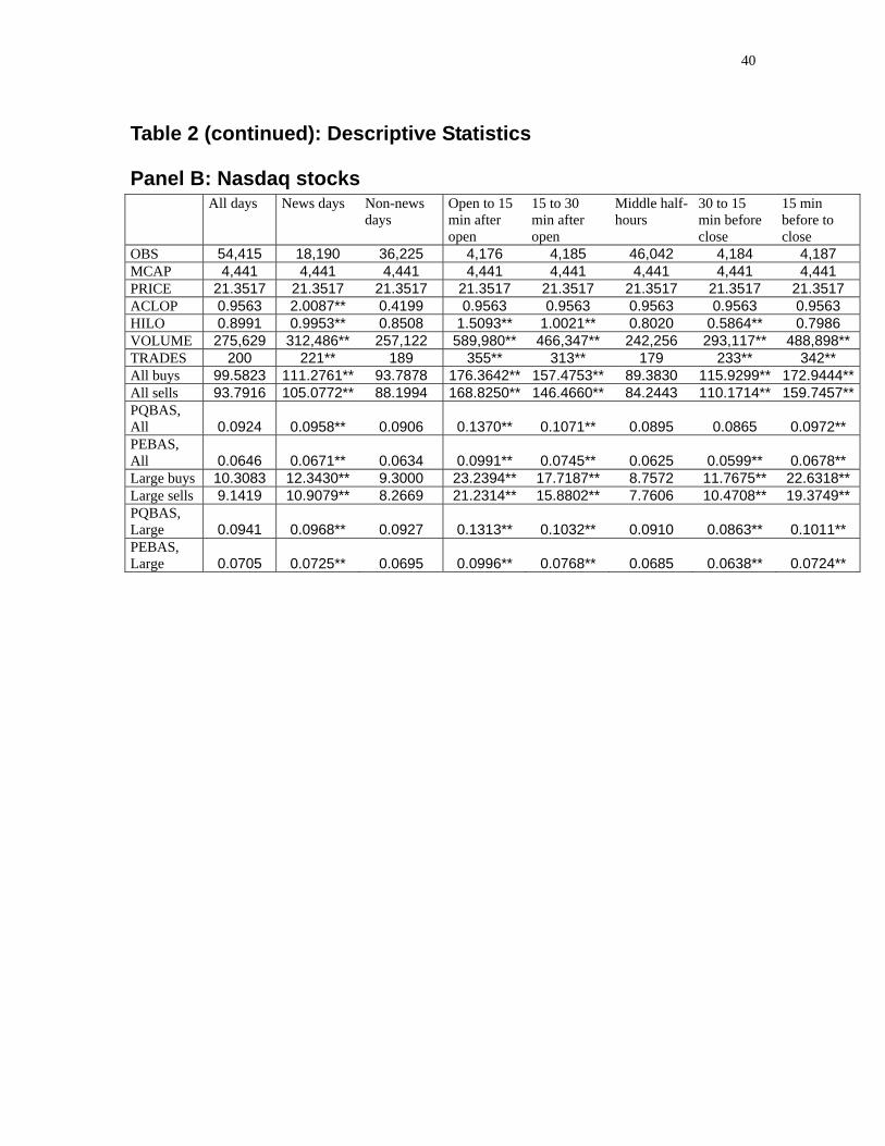
40
Table 2 (continued): Descriptive Statistics
Panel B: Nasdaq stocks All days News days Non-news
days Open to 15 min after open
15 to 30 min after open
Middle half-hours
30 to 15 min before close
15 min before to close
OBS 54,415 18,190 36,225 4,176 4,185 46,042 4,184 4,187 MCAP 4,441 4,441 4,441 4,441 4,441 4,441 4,441 4,441 PRICE 21.3517 21.3517 21.3517 21.3517 21.3517 21.3517 21.3517 21.3517 ACLOP 0.9563 2.0087** 0.4199 0.9563 0.9563 0.9563 0.9563 0.9563 HILO 0.8991 0.9953** 0.8508 1.5093** 1.0021** 0.8020 0.5864** 0.7986 VOLUME 275,629 312,486** 257,122 589,980** 466,347** 242,256 293,117** 488,898** TRADES 200 221** 189 355** 313** 179 233** 342** All buys 99.5823 111.2761** 93.7878 176.3642** 157.4753** 89.3830 115.9299** 172.9444**All sells 93.7916 105.0772** 88.1994 168.8250** 146.4660** 84.2443 110.1714** 159.7457**PQBAS, All
0.0924 0.0958** 0.0906
0.1370**
0.1071**
0.0895
0.0865
0.0972**
PEBAS, All
0.0646 0.0671** 0.0634
0.0991**
0.0745**
0.0625
0.0599**
0.0678**
Large buys 10.3083 12.3430** 9.3000 23.2394** 17.7187** 8.7572 11.7675** 22.6318** Large sells 9.1419 10.9079** 8.2669 21.2314** 15.8802** 7.7606 10.4708** 19.3749** PQBAS, Large
0.0941 0.0968** 0.0927
0.1313**
0.1032**
0.0910
0.0863**
0.1011**
PEBAS, Large
0.0705 0.0725** 0.0695
0.0996**
0.0768**
0.0685
0.0638**
0.0724**
41
Table 3: Tests of Independence of Buy and Sell Trade Arrivals The table shows, for each stock, results from tests of the null hypothesis that buyer- and seller-initiated trades in a half-hour interval are statistically independent. The statistical measures are computed separately for the sample of All trade sizes (All) and the sample of large trades (Large), defined as those in the top 10 percentile of the dollar value of trades of a stock. Buyer and seller initiated trades are determined using the Lee-Ready (1991) algorithm. We count the number of half-hour windows for which each combination of buy and sell triggered trades (e.g. two buy trades and one sell trade) was observed, and record them in a buy-sell (BSELL) matrix. Our null hypothesis is that the rows and columns of the BSELL matrix are not associated. To test the hypothesis, we use the Pearson chi-square statistic QP, which is equal to
( )∑∑
−=
i j ij
ijijP
nQ
εε 2 , where nij is the observed frequency of buy-triggered and sell-triggered trade arrivals in
row i and column j, the expected frequency (under the null hypothesis of independence) is nnn ji
ij..=ε ,
∑=j
iji nn . is the sum of elements in row i, ∑=
iijj nn.
is the sum of elements in column j, and ∑∑=i j
ijnn is the
overall total. When the rows and columns are independent, QP has an asymptotic chi-square distribution with (R-1)(C-1) degrees of freedom (DOF), where R is the number of rows and C is the number of columns in the matrix. The table also shows the correlation (Corrln) between the rows and columns of the BSELL matrix. Panel A shows results for NYSE stocks and Panel B for Nasdaq stocks. The sample is 41 NYSE and 41 Nasdaq stocks during January 2 to May 31 2003. The NYSE and Nasdaq stocks are matched according to their closing price and market value on December 31 2002.
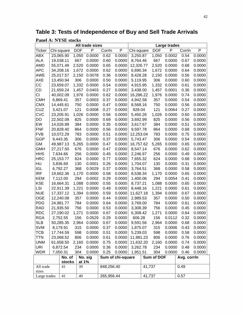
42
Table 3: Tests of Independence of Buy and Sell Trade Arrivals Panel A: NYSE stocks All trade sizes Large trades Ticker Chi-square DOF P Corrln P Chi-square DOF P Corrln P ABX 23,065.90 1,050 0.0000 0.62 0.0000 3,250.87 1,050 0.0002 0.54 0.0000ALA 19,038.11 667 0.0000 0.60 0.0000 8,764.46 667 0.0000 0.67 0.0000AMD 55,071.49 2,520 0.0000 0.65 0.0000 12,326.77 2,520 0.0000 0.68 0.0000APC 34,208.16 1,672 0.0000 0.62 0.0000 6,690.34 1,672 0.0000 0.64 0.0000AWE 25,017.57 2,150 0.0078 0.36 0.0000 8,428.28 2,150 0.0000 0.56 0.0000AXE 13,450.94 306 0.0000 0.50 0.0000 5,119.95 306 0.0000 0.60 0.0000CC 23,659.07 1,332 0.0000 0.54 0.0000 4,915.95 1,332 0.0000 0.61 0.0000CD 21,659.24 1,457 0.0403 0.27 0.0000 3,438.00 1,457 0.0001 0.36 0.0000CI 40,002.09 1,976 0.0000 0.62 0.0000 16,286.22 1,976 0.0000 0.74 0.0000CMH 6,869.41 357 0.0003 0.37 0.0000 4,942.58 357 0.0000 0.54 0.0000CMX 14,445.61 750 0.0000 0.47 0.0000 8,568.16 750 0.0000 0.56 0.0000CUZ 3,421.07 121 0.0008 0.27 0.0000 928.04 121 0.0064 0.27 0.0000CVC 23,205.91 1,026 0.0000 0.56 0.0000 5,450.26 1,026 0.0000 0.60 0.0000DO 22,502.08 825 0.0000 0.69 0.0000 3,692.99 825 0.0000 0.56 0.0000EW 14,026.89 384 0.0000 0.35 0.0000 3,617.67 384 0.0000 0.51 0.0000FNF 20,828.40 864 0.0000 0.56 0.0000 9,597.78 864 0.0000 0.68 0.0000FVB 10,072.29 783 0.0000 0.51 0.0000 12,253.04 783 0.0000 0.75 0.0000GGP 9,443.35 306 0.0000 0.37 0.0000 5,743.47 306 0.0000 0.54 0.0000GM 49,987.13 5,265 0.0000 0.47 0.0000 16,757.62 5,265 0.0000 0.65 0.0000GMH 27,217.50 676 0.0000 0.47 0.0000 8,547.14 676 0.0000 0.62 0.0000HHS 7,634.66 256 0.0000 0.45 0.0000 2,246.97 256 0.0000 0.49 0.0000HRC 25,153.77 624 0.0000 0.77 0.0000 7,655.32 624 0.0000 0.68 0.0000HU 3,836.69 130 0.0001 0.26 0.0000 1,704.07 130 0.0000 0.31 0.0000IGL 6,792.27 368 0.0029 0.37 0.0000 3,764.51 368 0.0000 0.58 0.0000IRF 19,662.36 1,170 0.0000 0.58 0.0000 8,538.34 1,170 0.0000 0.65 0.0000KEM 7,112.00 294 0.0002 0.29 0.0000 1,400.06 294 0.0054 0.41 0.0000KSE 16,664.31 1,088 0.0000 0.55 0.0000 8,737.21 1,088 0.0000 0.65 0.0000LSI 22,911.39 1,221 0.0000 0.49 0.0000 8,448.16 1,221 0.0000 0.61 0.0000NUE 17,337.12 1,394 0.0000 0.59 0.0000 11,627.18 1,394 0.0000 0.67 0.0000OGE 12,240.08 357 0.0000 0.44 0.0000 2,989.53 357 0.0000 0.50 0.0000PDG 24,981.77 784 0.0000 0.64 0.0000 3,769.00 784 0.0000 0.61 0.0000RAD 21,935.50 756 0.0000 0.53 0.0000 3,308.39 756 0.0000 0.45 0.0000RDC 27,190.02 1,271 0.0000 0.67 0.0000 6,308.42 1,271 0.0000 0.64 0.0000RGA 2,752.55 156 0.0529 0.29 0.0000 606.28 156 0.0112 0.32 0.0000SLB 50,285.35 2,964 0.0000 0.67 0.0000 9,591.56 2,964 0.0000 0.68 0.0000SVM 8,179.91 315 0.0000 0.37 0.0000 1,875.07 315 0.0006 0.43 0.0000TCB 17,744.59 598 0.0000 0.51 0.0000 5,239.03 598 0.0000 0.58 0.0000TTN 23,068.52 806 0.0000 0.61 0.0000 11,981.23 806 0.0000 0.76 0.0000UNM 61,658.50 2,160 0.0000 0.75 0.0000 11,632.20 2,160 0.0000 0.74 0.0000URI 6,872.54 234 0.0000 0.36 0.0000 3,262.78 234 0.0000 0.48 0.0000WDR 7,050.31 304 0.0000 0.25 0.0000 1,951.51 304 0.0000 0.46 0.0000 No. of
stocks No. sig at 1%
Sum of chi-square Sum of DOF Avg. corrln
All trade sizes
41 39 848,256.40 41,737 0.49
Large trades 41 40 265,956.44 41,737 0.57
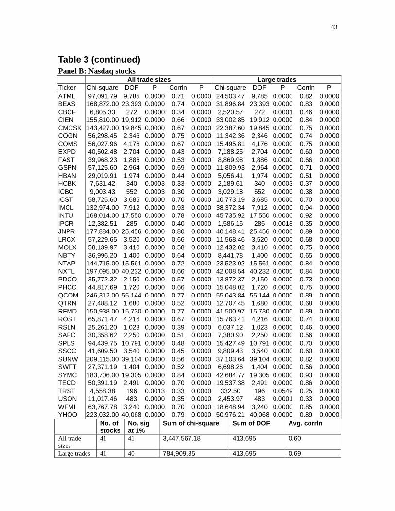
43
Table 3 (continued) Panel B: Nasdaq stocks All trade sizes Large trades Ticker Chi-square DOF P Corrln P Chi-square DOF P Corrln P ATML 97,091.79 9,785 0.0000 0.71 0.0000 24,503.47 9,785 0.0000 0.82 0.0000BEAS 168,872.00 23,393 0.0000 0.74 0.0000 31,896.84 23,393 0.0000 0.83 0.0000CBCF 6,805.33 272 0.0000 0.34 0.0000 2,520.57 272 0.0001 0.46 0.0000CIEN 155,810.00 19,912 0.0000 0.66 0.0000 33,002.85 19,912 0.0000 0.84 0.0000CMCSK 143,427.00 19,845 0.0000 0.67 0.0000 22,387.60 19,845 0.0000 0.75 0.0000COGN 56,298.45 2,346 0.0000 0.75 0.0000 11,342.36 2,346 0.0000 0.74 0.0000COMS 56,027.96 4,176 0.0000 0.67 0.0000 15,495.81 4,176 0.0000 0.75 0.0000EXPD 40,502.48 2,704 0.0000 0.43 0.0000 7,188.25 2,704 0.0000 0.60 0.0000FAST 39,968.23 1,886 0.0000 0.53 0.0000 8,869.98 1,886 0.0000 0.66 0.0000GSPN 57,125.60 2,964 0.0000 0.69 0.0000 11,809.93 2,964 0.0000 0.71 0.0000HBAN 29,019.91 1,974 0.0000 0.44 0.0000 5,056.41 1,974 0.0000 0.51 0.0000HCBK 7,631.42 340 0.0003 0.33 0.0000 2,189.61 340 0.0003 0.37 0.0000ICBC 9,003.43 552 0.0003 0.30 0.0000 3,029.18 552 0.0000 0.38 0.0000ICST 58,725.60 3,685 0.0000 0.70 0.0000 10,773.19 3,685 0.0000 0.70 0.0000IMCL 132,974.00 7,912 0.0000 0.93 0.0000 38,372.34 7,912 0.0000 0.94 0.0000INTU 168,014.00 17,550 0.0000 0.78 0.0000 45,735.92 17,550 0.0000 0.92 0.0000IPCR 12,382.51 285 0.0000 0.40 0.0000 1,586.16 285 0.0018 0.35 0.0000JNPR 177,884.00 25,456 0.0000 0.80 0.0000 40,148.41 25,456 0.0000 0.89 0.0000LRCX 57,229.65 3,520 0.0000 0.66 0.0000 11,568.46 3,520 0.0000 0.68 0.0000MOLX 58,139.97 3,410 0.0000 0.58 0.0000 12,432.02 3,410 0.0000 0.75 0.0000NBTY 36,996.20 1,400 0.0000 0.64 0.0000 8,441.78 1,400 0.0000 0.65 0.0000NTAP 144,715.00 15,561 0.0000 0.72 0.0000 23,523.02 15,561 0.0000 0.84 0.0000NXTL 197,095.00 40,232 0.0000 0.66 0.0000 42,008.54 40,232 0.0000 0.84 0.0000PDCO 35,772.32 2,150 0.0000 0.57 0.0000 13,872.37 2,150 0.0000 0.73 0.0000PHCC 44,817.69 1,720 0.0000 0.66 0.0000 15,048.02 1,720 0.0000 0.75 0.0000QCOM 246,312.00 55,144 0.0000 0.77 0.0000 55,043.84 55,144 0.0000 0.89 0.0000QTRN 27,488.12 1,680 0.0000 0.52 0.0000 12,707.45 1,680 0.0000 0.68 0.0000RFMD 150,938.00 15,730 0.0000 0.77 0.0000 41,500.97 15,730 0.0000 0.89 0.0000ROST 65,871.47 4,216 0.0000 0.67 0.0000 15,763.41 4,216 0.0000 0.74 0.0000RSLN 25,261.20 1,023 0.0000 0.39 0.0000 6,037.12 1,023 0.0000 0.46 0.0000SAFC 30,358.62 2,250 0.0000 0.51 0.0000 7,380.90 2,250 0.0000 0.56 0.0000SPLS 94,439.75 10,791 0.0000 0.48 0.0000 15,427.49 10,791 0.0000 0.70 0.0000SSCC 41,609.50 3,540 0.0000 0.45 0.0000 9,809.43 3,540 0.0000 0.60 0.0000SUNW 209,115.00 39,104 0.0000 0.56 0.0000 37,103.64 39,104 0.0000 0.82 0.0000SWFT 27,371.19 1,404 0.0000 0.52 0.0000 6,698.26 1,404 0.0000 0.56 0.0000SYMC 183,706.00 19,305 0.0000 0.84 0.0000 42,684.77 19,305 0.0000 0.93 0.0000TECD 50,391.19 2,491 0.0000 0.70 0.0000 19,537.38 2,491 0.0000 0.86 0.0000TRST 4,558.38 196 0.0013 0.33 0.0000 332.50 196 0.0549 0.25 0.0000USON 11,017.46 483 0.0000 0.35 0.0000 2,453.97 483 0.0001 0.33 0.0000WFMI 63,767.78 3,240 0.0000 0.70 0.0000 18,648.94 3,240 0.0000 0.85 0.0000YHOO 223,032.00 40,068 0.0000 0.79 0.0000 50,976.21 40,068 0.0000 0.89 0.0000 No. of
stocks No. sig at 1%
Sum of chi-square Sum of DOF Avg. corrln
All trade sizes
41 41 3,447,567.18 413,695 0.60
Large trades 41 40 784,909.35 413,695 0.69

44
Table 4: Distribution of buyer and seller-initiated trades Each cell of the table reports, averaged over stocks, and for a particular buy-and-sell-trade arrival combination, the observed and unexpected (in bold) percent of half-hour intervals with that combination, and the chi-square statistic of the cell as a percent of the overall chi-square. Numbers are reported for the following buy-and-sell-trade arrival combination: low buyer-initiated and low seller-initiated trade arrivals (LL), medium buyer-initiated and medium seller-initiated trade arrivals (MM), high buyer-initiated and low seller-initiated trade arrivals (HL), low buyer-initiated and high seller-initiated trade arrivals (LH), and high buyer-initiated and high seller-initiated trade arrivals (HH). Statistics are shown for different times of the day, and on days with news, and separately for the sample of all trade sizes (All) and the sample of large trades (Large), defined as those in the top 10 percentile of the dollar value of trades of a stock. Buyer and seller initiated trades are determined using the Lee-Ready (1991) algorithm. News days for a stock are the 30 percentile of days with the largest values of ACLOP, the absolute value of the excess returns from the previous day’s closing price to the current day’s opening price.
Details of the calculations are as follows. We first count the number of half-hour windows for which each combination of buy and sell triggered trades (e.g. two buy trades and one sell trade) was observed, and record them in a buy-sell (BSELL) matrix. Let nij denote the observed number of half-hours in cell (i, j) of the BSELL matrix. The expected number of half-hours in cell (i, j) is
nnn ji
ij..=ε , where ∑=
jiji nn .
is the sum
for row i, ∑=i
ijj nn.is the sum for column j, and ∑∑=
i jijnn is the overall total. The Pearson chi-square in
cell (i, j) is ( )ij
ijijij
nQ
εε 2−
= and the overall table chi-square QP is given by ( )∑∑
−=
i j ij
ijijP
nQ
εε 2 , so that the chi-
square contribution of cell (i, j) to QP is P
ijij Q
Q=χ . Finally, let oij, eij and uij be the observed, expected and
unexpected percent of half-hours in cell (i, j), where nn
o ijij =
, n
e ijij
ε= and
ijijij eou −= .
For each stock, the BSELL matrix is then mapped into a 3-by-3, High-Medium-Low (HML) matrix as follows. Assume that buy trades follow a Poisson arrival process, with parameter λb equal to the mean of the number of buy trades for the stock for a particular sample (e.g., all days or days with news). Then, for each stock and each sample, a half-hour interval with nb buy trades is mapped into the:
• LOW BUY cell if nb <= Rounddown(λb-√λb)
• HIGH BUY cell if nb > Roundup (λb+√λb)
• MEDIUM BUY cell in all other cases.
An identical procedure is carried out for sell trades, under the assumption that sell trades follow a Poisson arrival process, with parameter λs equal to the sample mean of the number of sell trades for the stock.
To obtain the observed and unexpected percent of trade arrivals, and the contribution of each cell to QP, we aggregate oij, eij and χij over the relevant cells of the BSELL matrix as determined by the mapping rule. For example, to obtain these numbers for the HH cell, we sum oij, uij and χij over all cells (i,j) of the BSELL matrix that are mapped into the HH cell of the HML matrix.
Results from hypotheses tests are shown under the heading, Mean Differences in Observed Percent of Half-Hours. We show t-statistics and p-values for the null hypotheses that the difference in means of observed percent of half-hours between different times of the day, and between news and non-news days, is zero (μ=0) for (1) the diagonal cells and (2) the HL and LH cells. The comparison is for stocks common to both samples. The standard errors used to compute the t-statistics are obtained from a Poisson regression of cell counts on cell and table dummies, as described in the Appendix. ** (*) indicates that the means are significantly different, at the one (five) percent level or less. The sample is 41 NYSE (Panel A) and 41 Nasdaq stocks (Panel B) during January 2 to May 31 2003. The NYSE and Nasdaq stocks are matched according to their closing price and market value on December 31 2002.
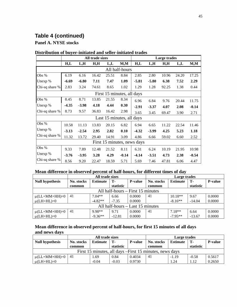
45
Table 4 (continued) Panel A. NYSE stocks Distribution of buyer-initiated and seller-initiated trades
All trade sizes Large trades H,L L,H H,H L,L M,M H,L L,H H,H L,L M,M
All half-hours Obs % 6.19 6.16 16.42 25.51 8.84 2.85 2.80 10.96 24.20 17.25 Unexp % -6.69 -6.80 7.11 7.47 1.09 -5.81 -5.80 6.38 7.52 2.29 Chi-sq share % 2.83 3.24 74.61 8.65 1.02 1.29 1.28 92.25 1.38 0.44
First 15 minutes, all days Obs % 8.45 8.71 13.85 21.55 8.34 6.96 6.84 9.76 20.44 11.75 Unexp % -4.35 -3.98 4.18 4.44 0.30 -2.91 -3.37 4.07 2.08 -0.14 Chi-sq share % 8.73 9.57 36.83 16.42 2.98 3.65 3.45 69.47 3.90 2.71
Last 15 minutes, all days Obs % 10.58 11.13 13.83 20.15 6.82 6.94 6.65 11.22 22.54 11.46 Unexp % -3.13 -2.54 2.95 2.82 0.10 -4.32 -3.99 4.25 5.23 1.18 Chi-sq share % 11.32 13.72 29.40 14.91 3.09 4.86 6.66 59.02 6.60 2.52
First 15 minutes, news days Obs % 9.33 7.89 12.48 21.52 8.11 6.31 6.24 10.19 21.95 10.98 Unexp % -3.76 -3.95 3.28 4.29 -0.14 -4.14 -3.51 4.73 2.38 -0.54 Chi-sq share % 8.56 9.20 22.47 18.59 5.71 5.69 7.46 47.81 6.06 4.47
Mean difference in observed percent of half-hours, for different times of day All trade sizes Large trades Null hypothesis No. stocks
common Estimate T-
statistic P-value No. stocks
common Estimate T-
statistic P-value
All half-hours – First 15 minutes μ(LL+MM+HH)=0 41 7.04** 6.66 0.0000 41 10.18** 9.67 0.0000 μ(LH+HL)=0 -4.82** -7.35 0.0000 -8.16** -14.04 0.0000
All half-hours – Last 15 minutes μ(LL+MM+HH)=0 41 9.98** 9.71 0.0000 41 7.18** 6.64 0.0000 μ(LH+HL)=0 -9.36** -12.81 0.0000 -7.95** -13.67 0.0000 Mean difference in observed percent of half-hours, for first 15 minutes of all days and news days All trade sizes Large trades Null hypothesis No. stocks
common Estimate T-
statistic P-value No. stocks
common Estimate T-
statistic P-value
First 15 minutes, all days –First 15 minutes, news days μ(LL+MM+HH)=0 41 1.69 0.84 0.4034 41 -1.19 -0.58 0.5617 μ(LH+HL)=0 -0.04 -0.03 0.9730 1.24 1.12 0.2650
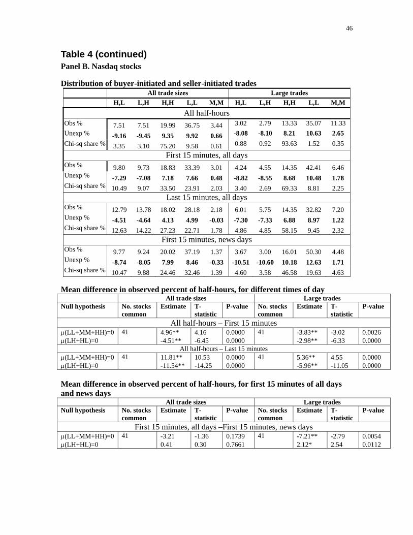
46
Table 4 (continued) Panel B. Nasdaq stocks Distribution of buyer-initiated and seller-initiated trades
All trade sizes Large trades H,L L,H H,H L,L M,M H,L L,H H,H L,L M,M
All half-hours Obs % 7.51 7.51 19.99 36.75 3.44 3.02 2.79 13.33 35.07 11.33 Unexp % -9.16 -9.45 9.35 9.92 0.66 -8.08 -8.10 8.21 10.63 2.65 Chi-sq share % 3.35 3.10 75.20 9.58 0.61 0.88 0.92 93.63 1.52 0.35
First 15 minutes, all days Obs % 9.80 9.73 18.83 33.39 3.01 4.24 4.55 14.35 42.41 6.46 Unexp % -7.29 -7.08 7.18 7.66 0.48 -8.82 -8.55 8.68 10.48 1.78 Chi-sq share % 10.49 9.07 33.50 23.91 2.03 3.40 2.69 69.33 8.81 2.25
Last 15 minutes, all days Obs % 12.79 13.78 18.02 28.18 2.18 6.01 5.75 14.35 32.82 7.20 Unexp % -4.51 -4.64 4.13 4.99 -0.03 -7.30 -7.33 6.88 8.97 1.22 Chi-sq share % 12.63 14.22 27.23 22.71 1.78 4.86 4.85 58.15 9.45 2.32
First 15 minutes, news days Obs % 9.77 9.24 20.02 37.19 1.37 3.67 3.00 16.01 50.30 4.48 Unexp % -8.74 -8.05 7.99 8.46 -0.33 -10.51 -10.60 10.18 12.63 1.71 Chi-sq share % 10.47 9.88 24.46 32.46 1.39 4.60 3.58 46.58 19.63 4.63
Mean difference in observed percent of half-hours, for different times of day All trade sizes Large trades Null hypothesis No. stocks
common Estimate T-
statistic P-value No. stocks
common Estimate T-
statistic P-value
All half-hours – First 15 minutes μ(LL+MM+HH)=0 41 4.96** 4.16 0.0000 41 -3.83** -3.02 0.0026 μ(LH+HL)=0 -4.51** -6.45 0.0000 -2.98** -6.33 0.0000
All half-hours – Last 15 minutes μ(LL+MM+HH)=0 41 11.81** 10.53 0.0000 41 5.36** 4.55 0.0000 μ(LH+HL)=0 -11.54** -14.25 0.0000 -5.96** -11.05 0.0000 Mean difference in observed percent of half-hours, for first 15 minutes of all days and news days All trade sizes Large trades Null hypothesis No. stocks
common Estimate T-
statistic P-value No. stocks
common Estimate T-
statistic P-value
First 15 minutes, all days –First 15 minutes, news days μ(LL+MM+HH)=0 41 -3.21 -1.36 0.1739 41 -7.21** -2.79 0.0054 μ(LH+HL)=0 0.41 0.30 0.7661 2.12* 2.54 0.0112
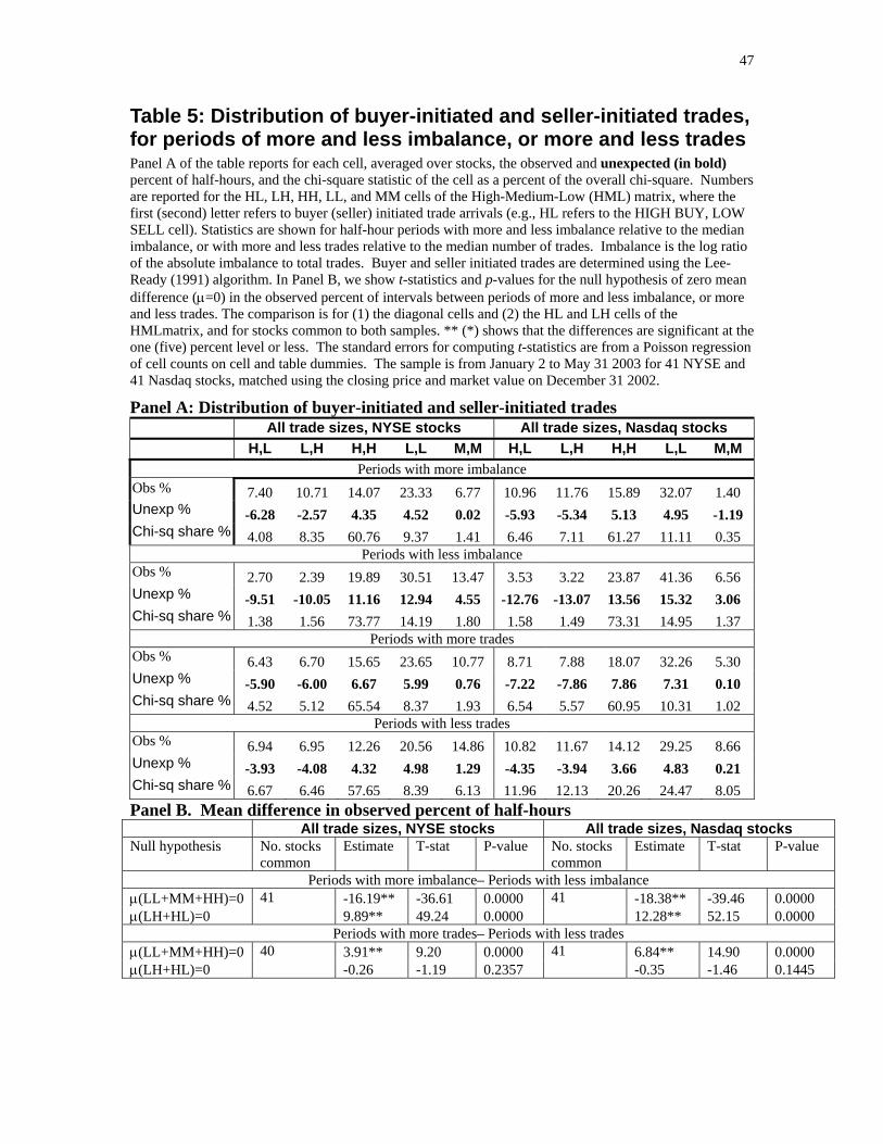
47
Table 5: Distribution of buyer-initiated and seller-initiated trades, for periods of more and less imbalance, or more and less trades Panel A of the table reports for each cell, averaged over stocks, the observed and unexpected (in bold) percent of half-hours, and the chi-square statistic of the cell as a percent of the overall chi-square. Numbers are reported for the HL, LH, HH, LL, and MM cells of the High-Medium-Low (HML) matrix, where the first (second) letter refers to buyer (seller) initiated trade arrivals (e.g., HL refers to the HIGH BUY, LOW SELL cell). Statistics are shown for half-hour periods with more and less imbalance relative to the median imbalance, or with more and less trades relative to the median number of trades. Imbalance is the log ratio of the absolute imbalance to total trades. Buyer and seller initiated trades are determined using the Lee-Ready (1991) algorithm. In Panel B, we show t-statistics and p-values for the null hypothesis of zero mean difference (μ=0) in the observed percent of intervals between periods of more and less imbalance, or more and less trades. The comparison is for (1) the diagonal cells and (2) the HL and LH cells of the HMLmatrix, and for stocks common to both samples. ** (*) shows that the differences are significant at the one (five) percent level or less. The standard errors for computing t-statistics are from a Poisson regression of cell counts on cell and table dummies. The sample is from January 2 to May 31 2003 for 41 NYSE and 41 Nasdaq stocks, matched using the closing price and market value on December 31 2002.
Panel A: Distribution of buyer-initiated and seller-initiated trades All trade sizes, NYSE stocks All trade sizes, Nasdaq stocks H,L L,H H,H L,L M,M H,L L,H H,H L,L M,M
Periods with more imbalance Obs % 7.40 10.71 14.07 23.33 6.77 10.96 11.76 15.89 32.07 1.40 Unexp % -6.28 -2.57 4.35 4.52 0.02 -5.93 -5.34 5.13 4.95 -1.19 Chi-sq share % 4.08 8.35 60.76 9.37 1.41 6.46 7.11 61.27 11.11 0.35
Periods with less imbalance Obs % 2.70 2.39 19.89 30.51 13.47 3.53 3.22 23.87 41.36 6.56 Unexp % -9.51 -10.05 11.16 12.94 4.55 -12.76 -13.07 13.56 15.32 3.06 Chi-sq share % 1.38 1.56 73.77 14.19 1.80 1.58 1.49 73.31 14.95 1.37
Periods with more trades Obs % 6.43 6.70 15.65 23.65 10.77 8.71 7.88 18.07 32.26 5.30 Unexp % -5.90 -6.00 6.67 5.99 0.76 -7.22 -7.86 7.86 7.31 0.10 Chi-sq share % 4.52 5.12 65.54 8.37 1.93 6.54 5.57 60.95 10.31 1.02
Periods with less trades Obs % 6.94 6.95 12.26 20.56 14.86 10.82 11.67 14.12 29.25 8.66 Unexp % -3.93 -4.08 4.32 4.98 1.29 -4.35 -3.94 3.66 4.83 0.21 Chi-sq share % 6.67 6.46 57.65 8.39 6.13 11.96 12.13 20.26 24.47 8.05 Panel B. Mean difference in observed percent of half-hours All trade sizes, NYSE stocks All trade sizes, Nasdaq stocks Null hypothesis No. stocks
common Estimate T-stat P-value No. stocks
common Estimate T-stat P-value
Periods with more imbalance– Periods with less imbalance μ(LL+MM+HH)=0 41 -16.19** -36.61 0.0000 41 -18.38** -39.46 0.0000 μ(LH+HL)=0 9.89** 49.24 0.0000 12.28** 52.15 0.0000
Periods with more trades– Periods with less trades μ(LL+MM+HH)=0 40 3.91** 9.20 0.0000 41 6.84** 14.90 0.0000 μ(LH+HL)=0 -0.26 -1.19 0.2357 -0.35 -1.46 0.1445

48
Table 6: Regressions of Volatility on Sidedness and Clustering The table shows results from a regression of volatility on dummy variables for sidedness and clustering. Statistics are reported separately for the sample of All trade sizes (All) and the sample of large trades (Large), defined as those in the top 10 percentile of the dollar value of trades of a stock in the sample. The sample is 41 NYSE (Panel A) and 41 Nasdaq (Panel B) stocks from January 2 to May 31 2003. The NYSE and Nasdaq stocks are matched according to their closing price and market value on December 31 2002. The proxy for volatility, the dependent variable, is HILO, equal to the log ratio of the highest to the lowest price in a half-hour interval. HILO is regressed on dummy variables for sidedness and clustering. They refer to cells in the 3x3 High-Medium-Low (HML) buy-sell matrix (e.g., HL refers to the HIGH BUY, LOW SELL cell), as follows:
DUMMY1: equals 1 if the half-hour interval falls in the LL cell
DUMMY2: equals 1 if the half-hour interval falls in the MM cell
DUMMY3: equals 1 if the half-hour interval falls in the LH or HL cells
DUMMY4: equals 1 if the half-hour interval falls in the MH or HM cells
DUMMY5: equals 1 if the half-hour interval falls in the HH cell
Buyer and seller initiated trades are determined using the Lee-Ready (1991) algorithm. The omitted cells are the (LM, ML) cells of the HML matrix.
In addition, HILO is regressed on the following control variables:
• Log of the number of trades in an interval
• IMBALANCE: log ratio of the absolute imbalance to the total number of trades, where imbalance is the number of buyer-initiated minus the number of seller-initiated trades
• NEWS: a dummy variable that equals 1 on days with news.
• [Open, 15 min after open]: a dummy variable that equals 1 when the trade occurs in the first 15 minutes of the trading day.
• [15 min to 30 min after open]: a dummy variable that equals 1 when the trade occurs from 15 to 30 minutes after the open.
• [30 min to 15 min before close]: a dummy variable that equals 1 when the trade occurs from 15 to 30 minutes before close.
• [15 min before close, close]: a dummy variable that equals 1 when the trade occurs in the last 15 minutes of the trading day.
• Log of the previous day’s closing price
• PEBAS: the proportional effective bid-ask half-spread, equal to Q*(P- M)/M, where P is the trade price, M is the quote mid-point, and Q is +1 (-1) for a buyer (seller) initiated trade.
• 3 lags of HILO. For the first-half hour of the day, we use as the first lag of HILO the absolute excess return from the previous day’s closing to the current day’s opening price.
Estimates have been multiplied by 100. T-statistics are corrected for autocorrelation and heteroskedasticity using the Newey-West estimator and 14 lags. A ** indicates significance at 1 per cent level or less; * indicates significance at 5 percent level or less.
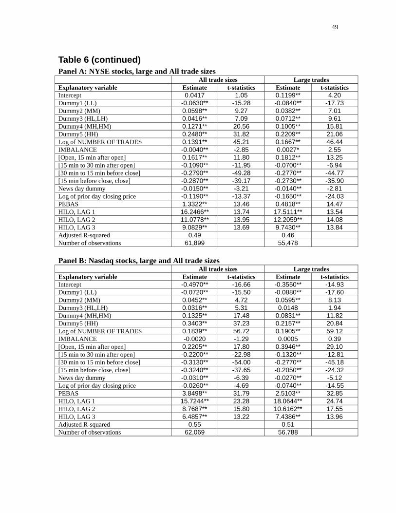
49
Table 6 (continued) Panel A: NYSE stocks, large and All trade sizes All trade sizes Large trades Explanatory variable Estimate t-statistics Estimate t-statistics Intercept 0.0417 1.05 0.1199** 4.20 Dummy1 (LL) -0.0630** -15.28 -0.0840** -17.73 Dummy2 (MM) 0.0598** 9.27 0.0382** 7.01 Dummy3 (HL,LH) 0.0416** 7.09 0.0712** 9.61 Dummy4 (MH,HM) 0.1271** 20.56 0.1005** 15.81 Dummy5 (HH) 0.2480** 31.82 0.2209** 21.06 Log of NUMBER OF TRADES 0.1391** 45.21 0.1667** 46.44 IMBALANCE -0.0040** -2.85 0.0027* 2.55 [Open, 15 min after open] 0.1617** 11.80 0.1812** 13.25 [15 min to 30 min after open] -0.1090** -11.95 -0.0700** -6.94 [30 min to 15 min before close] -0.2790** -49.28 -0.2770** -44.77 [15 min before close, close] -0.2870** -39.17 -0.2730** -35.90 News day dummy -0.0150** -3.21 -0.0140** -2.81 Log of prior day closing price -0.1190** -13.37 -0.1650** -24.03 PEBAS 1.3322** 13.46 0.4818** 14.47 HILO, LAG 1 16.2466** 13.74 17.5111** 13.54 HILO, LAG 2 11.0778** 13.95 12.2059** 14.08 HILO, LAG 3 9.0829** 13.69 9.7430** 13.84 Adjusted R-squared 0.49 0.46 Number of observations 61,899 55,478 Panel B: Nasdaq stocks, large and All trade sizes All trade sizes Large trades Explanatory variable Estimate t-statistics Estimate t-statistics Intercept -0.4970** -16.66 -0.3550** -14.93 Dummy1 (LL) -0.0720** -15.50 -0.0880** -17.60 Dummy2 (MM) 0.0452** 4.72 0.0595** 8.13 Dummy3 (HL,LH) 0.0316** 5.31 0.0148 1.94 Dummy4 (MH,HM) 0.1325** 17.48 0.0831** 11.82 Dummy5 (HH) 0.3403** 37.23 0.2157** 20.84 Log of NUMBER OF TRADES 0.1839** 56.72 0.1905** 59.12 IMBALANCE -0.0020 -1.29 0.0005 0.39 [Open, 15 min after open] 0.2205** 17.80 0.3946** 29.10 [15 min to 30 min after open] -0.2200** -22.98 -0.1320** -12.81 [30 min to 15 min before close] -0.3130** -54.00 -0.2770** -45.18 [15 min before close, close] -0.3240** -37.65 -0.2050** -24.32 News day dummy -0.0310** -6.39 -0.0270** -5.12 Log of prior day closing price -0.0260** -4.69 -0.0740** -14.55 PEBAS 3.8498** 31.79 2.5103** 32.85 HILO, LAG 1 15.7244** 23.28 18.0644** 24.74 HILO, LAG 2 8.7687** 15.80 10.6162** 17.55 HILO, LAG 3 6.4857** 13.22 7.4386** 13.96 Adjusted R-squared 0.55 0.51 Number of observations 62,069 56,788

50
Table 7: Regressions of Trading Costs on Sidedness and Clustering The table shows results from a regression of the trading costs on dummy variables for sidedness and clustering. The sample is 41 NYSE (Panel A) and 41 Nasdaq stocks (Panel B) during January 2 to May 31 2003. The NYSE and Nasdaq stocks are matched according to their closing price and market value on December 31 2002. Statistics are reported separately for the sample of All trade sizes (All) and the sample of large trades (Large), defined as those in the top 10 percentile of the dollar value of trades of a stock in the sample. The proxy for trading costs is PEBAS, the average proportional effective bid-ask half-spread in a half-hour interval. PEBAS is Q*(P- M)/M, where P is the trade price, Q is +1 (-1) for a buyer (seller) initiated trade, and M is the quote mid-point. The trading cost measure is regressed on dummy variables for sidedness and clustering. They refer to cells in the 3x3 High-Medium-Low (HML) buy-sell matrix (e.g., HH refers to the HIGH BUY, HIGH SELL cell), as follows:
DUMMY1: equals 1 if the half-hour interval falls in the LL cell
DUMMY2: equals 1 if the half-hour interval falls in the MM cell
DUMMY3: equals 1 if the half-hour interval falls in the LH or HL cells
DUMMY4: equals 1 if the half-hour interval falls in the MH or HM cells
DUMMY5: equals 1 if the half-hour interval falls in the HH cell
Buyer and seller initiated trades are determined using the Lee-Ready (1991) algorithm. The omitted cells are the (LM, ML) cells of the HML matrix.
In addition, the trading cost measure is regressed on the following control variables:
• Log of the number of trades in a half-hour interval
• IMBALANCE: log ratio of the absolute imbalance to the total number of trades, where imbalance is the number of buyer-initiated minus the number of seller-initiated trades
• NEWS: a dummy variable that equals 1 on days with news.
• [Open, 15 min after open]: a dummy variable that equals 1 when the trade occurs in the first 15 minutes of the trading day.
• [15 min to 30 min after open]: a dummy variable that equals 1 when the trade occurs from 15 to 30 minutes after the open.
• [30 min to 15 min before close]: a dummy variable that equals 1 when the trade occurs from 15 to 30 minutes before close.
• [15 min before close, close]: a dummy variable that equals 1 when the trade occurs in the last 15 minutes of the trading day.
• Log of the previous day’s closing price
• HILO: log ratio of the maximum to the minimum price in a half-hour interval
• 3 lags of PEBAS
Estimates have been multiplied by 100. T-statistics are corrected for autocorrelation and heteroskedasticity using the Newey-West procedure. A ** indicates significance at 1 per cent level or less; * indicates significance at 5 percent level or less.
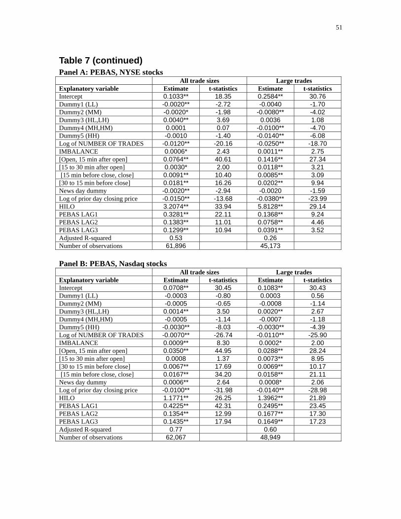
51
Table 7 (continued) Panel A: PEBAS, NYSE stocks All trade sizes Large trades Explanatory variable Estimate t-statistics Estimate t-statistics Intercept 0.1033** 18.35 0.2584** 30.76 Dummy1 (LL) -0.0020** -2.72 -0.0040 -1.70 Dummy2 (MM) -0.0020* -1.98 -0.0080** -4.02 Dummy3 (HL,LH) 0.0040** 3.69 0.0036 1.08 Dummy4 (MH,HM) 0.0001 0.07 -0.0100** -4.70 Dummy5 (HH) -0.0010 -1.40 -0.0140** -6.08 Log of NUMBER OF TRADES -0.0120** -20.16 -0.0250** -18.70 IMBALANCE 0.0006* 2.43 0.0011** 2.75 [Open, 15 min after open] 0.0764** 40.61 0.1416** 27.34 [15 to 30 min after open] 0.0030* 2.00 0.0118** 3.21 [15 min before close, close] 0.0091** 10.40 0.0085** 3.09 [30 to 15 min before close] 0.0181** 16.26 0.0202** 9.94 News day dummy -0.0020** -2.94 -0.0020 -1.59 Log of prior day closing price -0.0150** -13.68 -0.0380** -23.99 HILO 3.2074** 33.94 5.8128** 29.14 PEBAS LAG1 0.3281** 22.11 0.1368** 9.24 PEBAS LAG2 0.1383** 11.01 0.0758** 4.46 PEBAS LAG3 0.1299** 10.94 0.0391** 3.52 Adjusted R-squared 0.53 0.26 Number of observations 61,896 45,173 Panel B: PEBAS, Nasdaq stocks All trade sizes Large trades Explanatory variable Estimate t-statistics Estimate t-statistics Intercept 0.0708** 30.45 0.1083** 30.43 Dummy1 (LL) -0.0003 -0.80 0.0003 0.56 Dummy2 (MM) -0.0005 -0.65 -0.0008 -1.14 Dummy3 (HL,LH) 0.0014** 3.50 0.0020** 2.67 Dummy4 (MH,HM) -0.0005 -1.14 -0.0007 -1.18 Dummy5 (HH) -0.0030** -8.03 -0.0030** -4.39 Log of NUMBER OF TRADES -0.0070** -26.74 -0.0110** -25.90 IMBALANCE 0.0009** 8.30 0.0002* 2.00 [Open, 15 min after open] 0.0350** 44.95 0.0288** 28.24 [15 to 30 min after open] 0.0008 1.37 0.0073** 8.95 [30 to 15 min before close] 0.0067** 17.69 0.0069** 10.17 [15 min before close, close] 0.0167** 34.20 0.0158** 21.11 News day dummy 0.0006** 2.64 0.0008* 2.06 Log of prior day closing price -0.0100** -31.98 -0.0140** -28.98 HILO 1.1771** 26.25 1.3962** 21.89 PEBAS LAG1 0.4225** 42.31 0.2495** 23.45 PEBAS LAG2 0.1354** 12.99 0.1677** 17.30 PEBAS LAG3 0.1435** 17.94 0.1649** 17.23 Adjusted R-squared 0.77 0.60 Number of observations 62,067 48,949
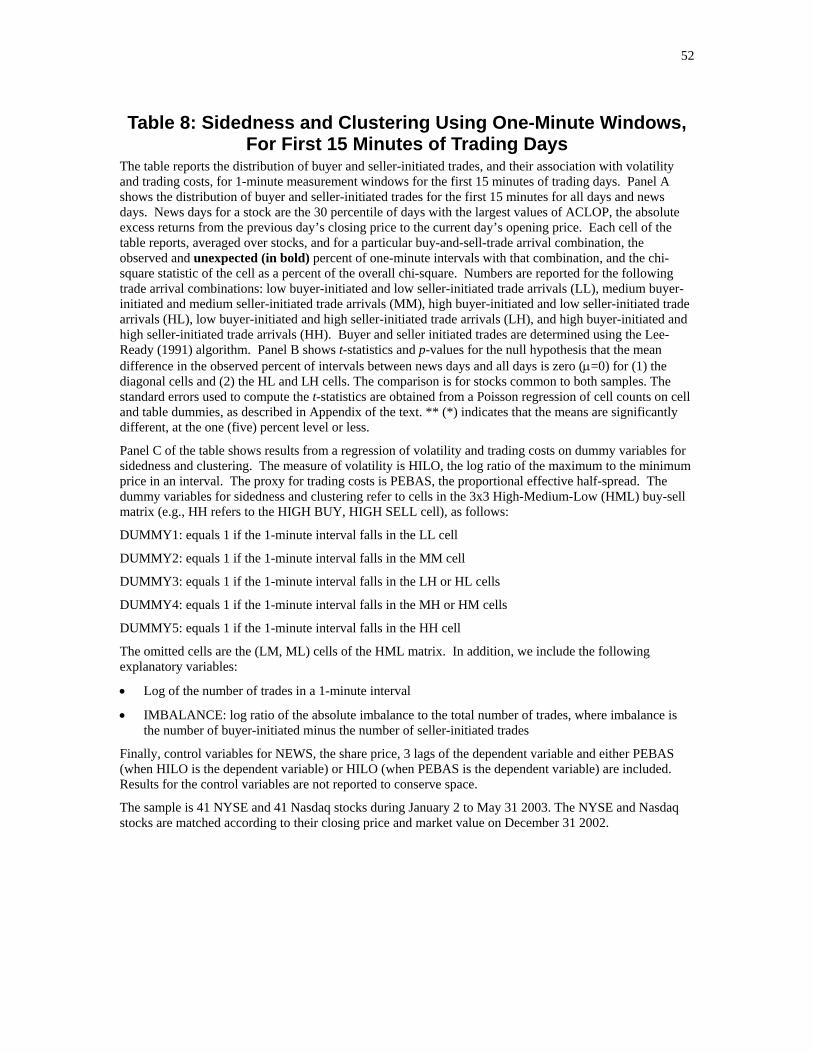
52
Table 8: Sidedness and Clustering Using One-Minute Windows, For First 15 Minutes of Trading Days
The table reports the distribution of buyer and seller-initiated trades, and their association with volatility and trading costs, for 1-minute measurement windows for the first 15 minutes of trading days. Panel A shows the distribution of buyer and seller-initiated trades for the first 15 minutes for all days and news days. News days for a stock are the 30 percentile of days with the largest values of ACLOP, the absolute excess returns from the previous day’s closing price to the current day’s opening price. Each cell of the table reports, averaged over stocks, and for a particular buy-and-sell-trade arrival combination, the observed and unexpected (in bold) percent of one-minute intervals with that combination, and the chi-square statistic of the cell as a percent of the overall chi-square. Numbers are reported for the following trade arrival combinations: low buyer-initiated and low seller-initiated trade arrivals (LL), medium buyer-initiated and medium seller-initiated trade arrivals (MM), high buyer-initiated and low seller-initiated trade arrivals (HL), low buyer-initiated and high seller-initiated trade arrivals (LH), and high buyer-initiated and high seller-initiated trade arrivals (HH). Buyer and seller initiated trades are determined using the Lee-Ready (1991) algorithm. Panel B shows t-statistics and p-values for the null hypothesis that the mean difference in the observed percent of intervals between news days and all days is zero (μ=0) for (1) the diagonal cells and (2) the HL and LH cells. The comparison is for stocks common to both samples. The standard errors used to compute the t-statistics are obtained from a Poisson regression of cell counts on cell and table dummies, as described in Appendix of the text. ** (*) indicates that the means are significantly different, at the one (five) percent level or less.
Panel C of the table shows results from a regression of volatility and trading costs on dummy variables for sidedness and clustering. The measure of volatility is HILO, the log ratio of the maximum to the minimum price in an interval. The proxy for trading costs is PEBAS, the proportional effective half-spread. The dummy variables for sidedness and clustering refer to cells in the 3x3 High-Medium-Low (HML) buy-sell matrix (e.g., HH refers to the HIGH BUY, HIGH SELL cell), as follows:
DUMMY1: equals 1 if the 1-minute interval falls in the LL cell
DUMMY2: equals 1 if the 1-minute interval falls in the MM cell
DUMMY3: equals 1 if the 1-minute interval falls in the LH or HL cells
DUMMY4: equals 1 if the 1-minute interval falls in the MH or HM cells
DUMMY5: equals 1 if the 1-minute interval falls in the HH cell
The omitted cells are the (LM, ML) cells of the HML matrix. In addition, we include the following explanatory variables:
• Log of the number of trades in a 1-minute interval
• IMBALANCE: log ratio of the absolute imbalance to the total number of trades, where imbalance is the number of buyer-initiated minus the number of seller-initiated trades
Finally, control variables for NEWS, the share price, 3 lags of the dependent variable and either PEBAS (when HILO is the dependent variable) or HILO (when PEBAS is the dependent variable) are included. Results for the control variables are not reported to conserve space.
The sample is 41 NYSE and 41 Nasdaq stocks during January 2 to May 31 2003. The NYSE and Nasdaq stocks are matched according to their closing price and market value on December 31 2002.
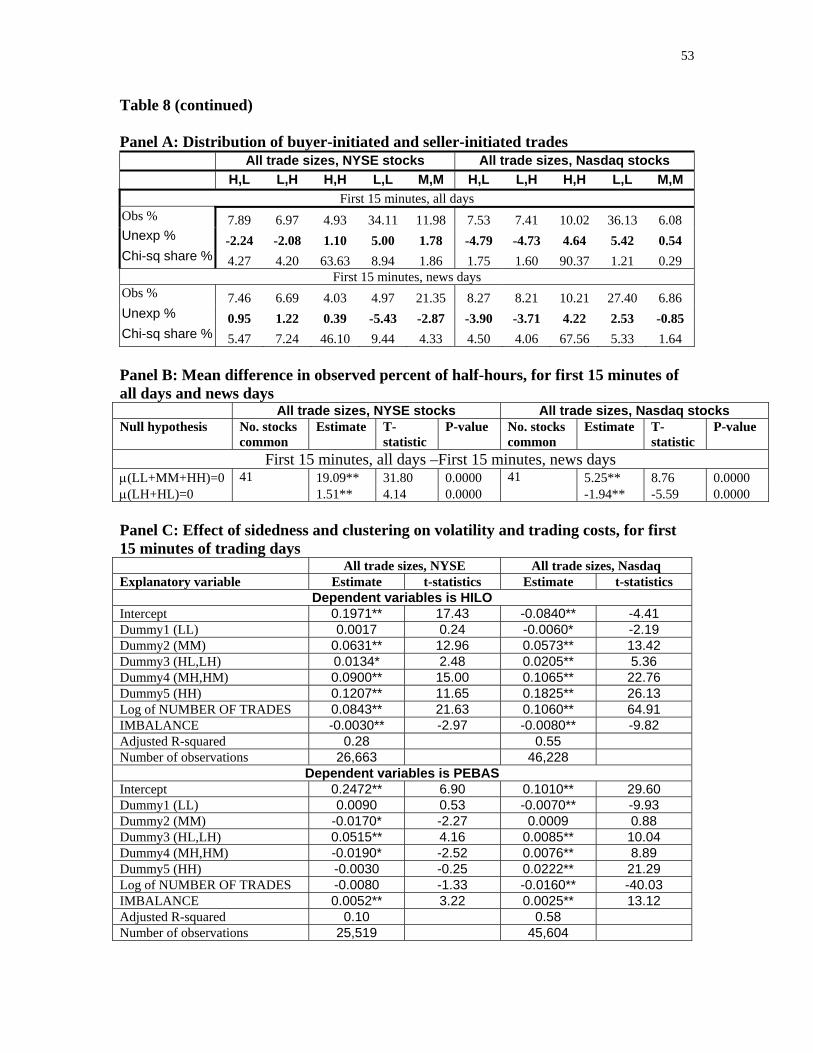
53
Table 8 (continued) Panel A: Distribution of buyer-initiated and seller-initiated trades All trade sizes, NYSE stocks All trade sizes, Nasdaq stocks H,L L,H H,H L,L M,M H,L L,H H,H L,L M,M
First 15 minutes, all days Obs % 7.89 6.97 4.93 34.11 11.98 7.53 7.41 10.02 36.13 6.08 Unexp % -2.24 -2.08 1.10 5.00 1.78 -4.79 -4.73 4.64 5.42 0.54 Chi-sq share % 4.27 4.20 63.63 8.94 1.86 1.75 1.60 90.37 1.21 0.29
First 15 minutes, news days Obs % 7.46 6.69 4.03 4.97 21.35 8.27 8.21 10.21 27.40 6.86 Unexp % 0.95 1.22 0.39 -5.43 -2.87 -3.90 -3.71 4.22 2.53 -0.85 Chi-sq share % 5.47 7.24 46.10 9.44 4.33 4.50 4.06 67.56 5.33 1.64 Panel B: Mean difference in observed percent of half-hours, for first 15 minutes of all days and news days All trade sizes, NYSE stocks All trade sizes, Nasdaq stocks Null hypothesis No. stocks
common Estimate T-
statistic P-value No. stocks
common Estimate T-
statistic P-value
First 15 minutes, all days –First 15 minutes, news days μ(LL+MM+HH)=0 41 19.09** 31.80 0.0000 41 5.25** 8.76 0.0000 μ(LH+HL)=0 1.51** 4.14 0.0000 -1.94** -5.59 0.0000 Panel C: Effect of sidedness and clustering on volatility and trading costs, for first 15 minutes of trading days All trade sizes, NYSE All trade sizes, Nasdaq Explanatory variable Estimate t-statistics Estimate t-statistics
Dependent variables is HILO Intercept 0.1971** 17.43 -0.0840** -4.41 Dummy1 (LL) 0.0017 0.24 -0.0060* -2.19 Dummy2 (MM) 0.0631** 12.96 0.0573** 13.42 Dummy3 (HL,LH) 0.0134* 2.48 0.0205** 5.36 Dummy4 (MH,HM) 0.0900** 15.00 0.1065** 22.76 Dummy5 (HH) 0.1207** 11.65 0.1825** 26.13 Log of NUMBER OF TRADES 0.0843** 21.63 0.1060** 64.91 IMBALANCE -0.0030** -2.97 -0.0080** -9.82 Adjusted R-squared 0.28 0.55 Number of observations 26,663 46,228
Dependent variables is PEBAS Intercept 0.2472** 6.90 0.1010** 29.60 Dummy1 (LL) 0.0090 0.53 -0.0070** -9.93 Dummy2 (MM) -0.0170* -2.27 0.0009 0.88 Dummy3 (HL,LH) 0.0515** 4.16 0.0085** 10.04 Dummy4 (MH,HM) -0.0190* -2.52 0.0076** 8.89 Dummy5 (HH) -0.0030 -0.25 0.0222** 21.29 Log of NUMBER OF TRADES -0.0080 -1.33 -0.0160** -40.03 IMBALANCE 0.0052** 3.22 0.0025** 13.12 Adjusted R-squared 0.10 0.58 Number of observations 25,519 45,604
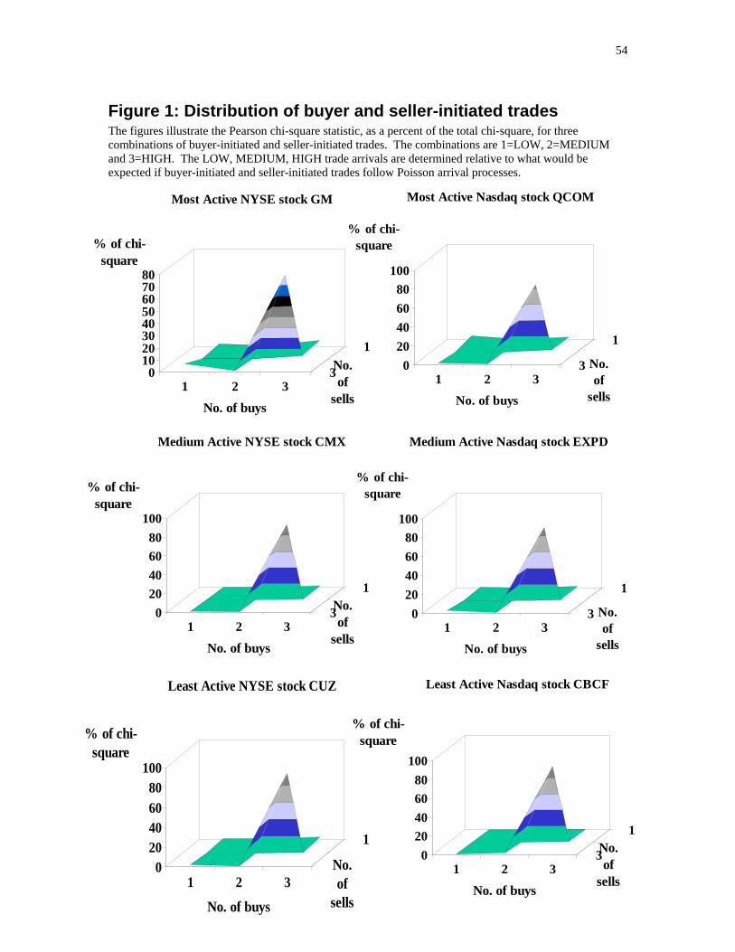
54
Figure 1: Distribution of buyer and seller-initiated trades The figures illustrate the Pearson chi-square statistic, as a percent of the total chi-square, for three combinations of buyer-initiated and seller-initiated trades. The combinations are 1=LOW, 2=MEDIUM and 3=HIGH. The LOW, MEDIUM, HIGH trade arrivals are determined relative to what would be expected if buyer-initiated and seller-initiated trades follow Poisson arrival processes.
01020304050607080
% of chi-square
1 2 3
1
3
No. of buys
No. of
sells
Most Active NYSE stock GM
020406080
100
% of chi-square
1 2 3
1
3
No. of buys
No. of
sells
Most Active Nasdaq stock QCOM
020406080
100
% of chi-square
1 2 3
1
3
No. of buys
No. of
sells
Medium Active NYSE stock CMX
020406080
100
% of chi-square
1 2 3
1
3
No. of buys
No. of
sells
Medium Active Nasdaq stock EXPD
020406080
100
% of chi-square
1 2 3
1
No.
Least Active NYSE stock CUZ
020406080
100
% of chi-square
1 2 3
1
3No. of
Least Active Nasdaq stock CBCF
No. of buyssells
No. of buysof
sells