DDEEPPOOCCEENN Working Paper Series No. 2008/28

Economic-Environmental Impact Analysis Based on a Bi-region Interregional I-O Model for Vietnam

Bui Trinh * Francisco T. Secretario **

Kim Kwangmun *** Le Ha Thanh ****

Pham Huong Giang ****

* I-O research Consultant, General Statistics Office, VIETNAM ** I-O Research Consultant, PHILIPPINES *** Toyohashi University of Technology, JAPAN **** Hanoi National Economic University, VIETNAM The DEPOCEN WORKING PAPER SERIES disseminates research findings and promotes scholar exchanges in all branches of economic studies, with a special emphasis on Vietnam. The views and interpretations expressed in the paper are those of the author(s) and do not necessarily represent the views and policies of the DEPOCEN or its Management Board. The DEPOCEN does not guarantee the accuracy of findings, interpretations, and data associated with the paper, and accepts no responsibility whatsoever for any consequences of their use. The author(s) remains the copyright owner. DEPOCEN WORKING PAPERS are available online at http://www.depocenwp.org

1

Economic-Environmental Impact Analysis Based on a Bi-region Interregional I-O Model for Vietnam,

between HoChiMinh City (HCMC) and the rest of Vietnam (ROV), 2000

By:

Bui Trinh I-O research Consultant, General Statistics Office, VIETNAM

E-mail: trinhcan@hotmail.comAddress: 2, Hoang Van Thu Str – Hanoi.

Tel: +8-48-431218

Francisco T. Secretario (presenter) I-O Research Consultant, PHILIPPINES

E-mail: ftsecret@yahoo.comPostal: L1, B3, RH2, Pilot Drive, Quezon City

Tel/Fax: +632-4362084

Kim Kwangmun Toyohashi University of Technology, JAPAN

Tenpaku-cho 1-1, Toyohasi-city, JAPAN Tel: +81-53-244-6842

Email: kim@tutrp.tut.ac.jp

Le Ha Thanh Hanoi National Economic University, VIETNAM

E-mail: thanhngaboss@yahoo.com

Pham Huong Giang Hanoi National Economic University, VIETNAM

E-mail: morningstar4321@yahoo.com

1. Introduction The structure of interregional linkages have been common topics of discussion in regional analysis; attention has been directed to problems of interregional feedback effects and the degree to which change originating in one region has capacity to influence activity levels in another region, in turn, will effect activity back in the region of origin.

While Miller (1966, 1969) proposed a formulation of the feedback process to handle this problem, Miyazawa suggested an innovative way of partitioning the system of regions that resulted in the identification of what are now referred to as internal, external multipliers interregional feedback effects.

From time to time, Input – Output model systems have been applied in estimating economic – environment linkages. Further, the economic interregional input output model system can be applied in analysis impacts on residuals generated by interregional economic activities.

This problems will processed with case study of HoChiMinh City (HCMC) and the Rest of Vietnam (ROV) based on interregional input output approach. The Vietnam interregional input output table constructed by the hybrid approach from National competitive input output table and HoChiMinh competitive input output table in 2000. The national IO tables was compiled by Vietnam General Statistical Office (GSO) and published in 2003, The HoChiMinh input output table was compiled as a joint undertaking between HCMC Province statistical Office GSO with financial assistance provided by the HCMC’s people and Provincial committees. This particular study was made possible with the availability of the just-completed research project on the compilation of the 2000 Bi-region Inter-Regional IO (IRIO) Table for the Vietnamese economy, with HoChiMinh City as the area of interest. As

2

such, this two-region table specifically divided the country into: Region 1 - HoChiMinh City, and Region 2 – the Rest of Viet Nam. The resulting IRIO table shows, in its compact form, the intra- as well as the inter-regional economic transactions at the two-region level of spatial delineation.

The first part of this paper presents the conceptual and accounting framework of the IRIO model in inter-regional economic impact analysis. In this paper, special attention is paid of the Miyazawa system in the decomposition of the economic multiplier effects. For the purpose of this study, the IO model is being extended to be able to measure economic-environmental linkages.

The second part is a case study for HoChiMinh City based on the 2000 IRIO table. The objective of this study is to measure the inter-regional, inter-industrial interdependencies as well as the consequent environmental effects of pollution emissions due to economic activities. An analysis of the empirical results on the economic-environmental multipliers is shown in the last part of this case study.

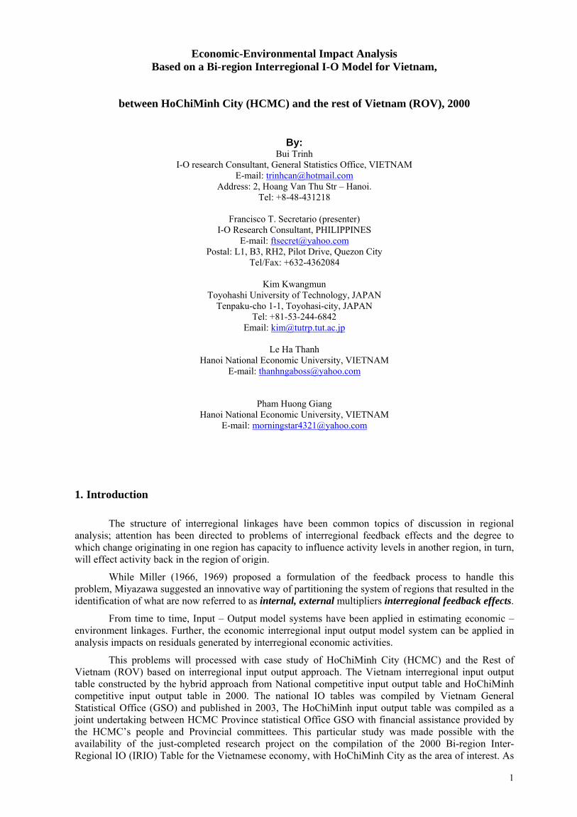
2. Overview 2.1. Major Socio-Economic Indicators

The following are some of the major socio-economic indicators at the national and sub-national level of geographic classification:

Table 1. Major Socio-Economic Indicators: Viet Nam YEAR

Major Indicators 1990 1995 1996 2000 1) AREA (Sq. Km.) VIET NAM 330,991 HO CHI MINH 2,095 REST OF VIET NAM 328,896

2) POPULATION (000 Persons) VIET NAM 66,016 71,995 73,157 77,635 HO CHI MINH 4,118 4,640 4,749 5,175 REST OF VIET NAM 61,898 67,355 68,408 72,460

3) POPULATION DENSITY (Persons/Sq Km) VIET NAM 199.4 217.5 221.0 234.6

HO CHI MINH 1,965.6 2,214.8 2,266.8 2,470.2 REST OF VIET NAM 188.2 204.8 208.0 220.3

4) EMPLOYMENT (000 Persons) VIET NAM 29,412 33,030 33,761 36,702 HO CHI MINH 1,529 1,821 1,895 2,237 REST OF VIET NAM 27,883 31,209 31,866 34,465

5) GDP (Billion Dong at Current Prices) VIET NAM 41,955 228,892 272,036 441,646 HO CHI MINH 6,770 36,975 45,545 75,444 REST OF VIET NAM 35,185 191,917 226,491 366,202

6) GDP (Bill. Dong At Constant 1994 Prices) VIET NAM 131,968 195,567 213,833 273,666 HO CHI MINH 17,993 32,596 37,380 52,228 REST OF VIET NAM 113,975 162,971 176,453 221,438

7) PER CAPITA GDP (000 Dong, current prices) VIET NAM 635.5 3,179.3 3,718.5 5,688.7

HO CHI MINH 1,644.0 7,968.8 9,590.4 14,578.6 REST OF VIET NAM 568.4 2,849.3 3,310.9 5,053.9

Source of Basic Data: GENERAL STATISTICS OFFICE

3

2.2. HoChiMinh City status 2.2.1. HoChiMinh City as Viet Nam’s Principal Trading Center

HoChiMinh city is one of the biggest cities in Viet Nam with a large area and crowded population, lies between the Mekong River Delta and Eastern Nam Bo. HoChiMinh city is the most important commercial center and the second most important political center of the country next to the capital of Hanoi. This city has good conditions on transportation, especially for airway and seaway, for example, Tan Son Nhat airport. So it is very convenient to undertake trading or exchange relations with the rest of Viet Nam (ROV) and the rest of the World (ROW) too. There are a lot of economic activities taking place here everyday. Like other places, HoChiMinh city not only use its own products but also products from other provinces and from the rest of the World for its intermediate and final consumption demands. It means that this city import products from other places and export products to the rest of the economy as well as to the rest of the World. It imports products not only for its own use but also for other provinces. In short, HoChiMinh City is the main transit point for imports required by other provinces. Similarly, HoChiMinh city is the principal transit point for exports coming from other provinces to foreign countries and to other provinces as well. The reason for choosing HoChiMinh city as the principal intermediate transit point in Viet Nam is because HoChiMinh City has the best transportation facilities, whether by sea or air, to carry out export-import economic activities.

2.2.2. Current status of water pollution in HoChiMinh City. HoChiMinh city is an important center for culture, economy and trade and international exchange. It also faces a big water pollution problem due to domestic and industrial wastewater. HoChiMinh city is located in the transitional zone of the east southern region and the Cuu Long River Delta. The river and canal system in HoChiMinh city is influenced by the semidiurnal solar tide. The level of tides is highest in October-November and lowest in June-July. Intrusion of saline water by tide influences the whole river and canal system. The population of HoChiMinh City is more than 5.1 million inhabitants, accounting for about 6% of the country’s total population. On the other hand, the industrial production of the city accounts for third of the whole country’s industrial production. HoChiMinh city has more than 680 factories/plants of which 500 are in the inner city. It has approximately 22 industrial zones: the main industries include textile, paper, food, chemical, sugar, soap, detergent, beverages, plastic, rubber, machines. In addition HoChiMinh city has almost 24.000 small-scale industrial companies, of which 89% are located in the residential areas of the inner city. There is no wastewater treatment plant in almost all existing factories. All the wastewater is discharged directly into the sewerage system of the city or into the receiving bodies. The flow rate of industrial wastewater is smaller than that of domestic wastewater but the pollutant concentration of the former is much higher and more dangerous. The factories and small scale industries in the city contribute significantly to the economy, but they also significantly pollute the environment. The water pollution can be classified into seven types: (1) Organic pollution, (2) Bacterial pollution, (3) Suspended solid pollution, (4) Nutrient pollution, (5) Pesticide pollution, (6) Heavy pollution, and (7) Oil pollution. 2.3. Overview of National, Regional and Input-Output Accounts Compilation in Viet Nam

2.3.1. National Accounts In line with Vietnam’s transition to market economy in 1986, the GSO shifted its framework of compiling the country’s economic accounts from the Material Product System (MPS) to the U.N. System of National Accounts (SNA). As shown in Table 2, the GSO through its National Accounts Department (NAD) started compiling the country’s annual national accounts based on the UNSNA in the early 1990s. This initial activity was made possible with technical and financial assistance provided by UNDP. Later on, ADB provided technical assistance grant to help improve the compilation of the national accounts including the construction of I/O tables. Currently available are national accounts time-series data from 1986 onwards. Compilation of quarterly national accounts started only in 1998.

2.3.2. Regional GDP At the regional level, the NAD started compiling regional GDP in 1993 based on data provided by Provincial Statistical Offices (PSO). Currently, the country is divided into 8 economic regions as shown as bellow: Red river Delta, North East, South Central Coast, Central highlands, North East South, North West, North Central Coast, and Mekong River Delta.

4

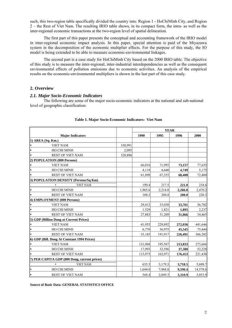
2.3.3. National I/O Tables Compilation of national I/O tables started also in the early 1990s with the compilation of the 1989 benchmark I/O table. The latest national I/O table relates to CY 2000 with sectorail dimension of 112 production sectors, 6 final demand and 4 primary input (or value added) components. In between 1989, 1996 and 2000, annual I/O updating had been also undertaken to provide users with more current I/O data. Currently, the national I/O table is of the competitive-imports type wherein no distinction is made between local and imported inputs. Due to lack of data on import transactions, the compilation of non-competitive I/O tables has been deferred. It is, however, expected that NAD’s ongoing activity of compiling the 2005 national I/O table will be able to compile an import matrix in order to generate a non-competitive type of I/O table. I/O analysis yields more meaningful results by using the non-competitive type.

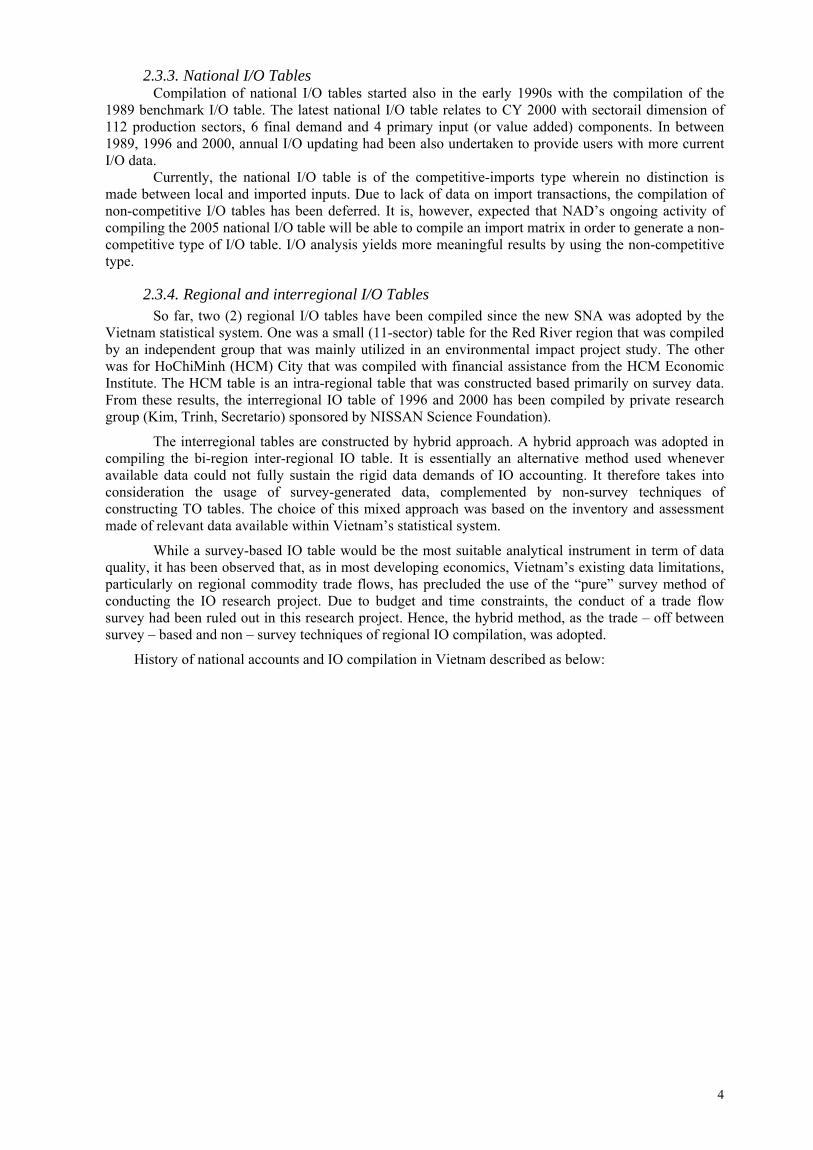
2.3.4. Regional and interregional I/O Tables So far, two (2) regional I/O tables have been compiled since the new SNA was adopted by the

Vietnam statistical system. One was a small (11-sector) table for the Red River region that was compiled by an independent group that was mainly utilized in an environmental impact project study. The other was for HoChiMinh (HCM) City that was compiled with financial assistance from the HCM Economic Institute. The HCM table is an intra-regional table that was constructed based primarily on survey data. From these results, the interregional IO table of 1996 and 2000 has been compiled by private research group (Kim, Trinh, Secretario) sponsored by NISSAN Science Foundation).

The interregional tables are constructed by hybrid approach. A hybrid approach was adopted in compiling the bi-region inter-regional IO table. It is essentially an alternative method used whenever available data could not fully sustain the rigid data demands of IO accounting. It therefore takes into consideration the usage of survey-generated data, complemented by non-survey techniques of constructing TO tables. The choice of this mixed approach was based on the inventory and assessment made of relevant data available within Vietnam’s statistical system.

While a survey-based IO table would be the most suitable analytical instrument in term of data quality, it has been observed that, as in most developing economics, Vietnam’s existing data limitations, particularly on regional commodity trade flows, has precluded the use of the “pure” survey method of conducting the IO research project. Due to budget and time constraints, the conduct of a trade flow survey had been ruled out in this research project. Hence, the hybrid method, as the trade – off between survey – based and non – survey techniques of regional IO compilation, was adopted.

History of national accounts and IO compilation in Vietnam described as below:

Table 2. History of National Accounts and I/O Compilation in Viet Nam

Type of Start of Compilation Frequency of

Economic Account ( based on SNA ) Compilation Compiler 1) National Accounts a) Annual 1992 ( UNDP sponsored) annual SNA Dept., GSO b) Quarterly 1998 quarterly SNA Dept., GSO 2) Regional GDP 1993 annual SNA Dept., GSO 3) National IO Tables a) Benchmark 1989 1996,2000 SNA Dept., GSO b) I/O Update Annual updating starting in 1990 SNA Dept., GSO 4) Regional I/O Tables

HO CHI MINH 1996 2000

Economic Institute of HCM,

HCM PSO

Red River Delta Region 1996 one-time Project Staff, LOICZ

Project 5) Interregional I/O Tables

HO CHI MINH City-The rest of Vietnam 1996 2000 Private researcher group,

NISSAN project (*) Private research group and NISSAN project’s research team include Dr.Kim Kwang Moon

(Toyohashi University of Technology, Japan), Mr.Francisco T. Secretario (Former ADB Expert, Philippine) and Bui Trinh (GSO, Vietnam), Hoang Tri (CERE, Vietnam); Dr.Kim Kwang Moon is team leader

3. Methodology 3.1. Enlarged Leontief Inverse and Internal and External Multipliers

As in national IO models, the basic relationship in intra-regional IO models is:

XYAX =+ or YXAI =− ).( (1)

Assume a two – fold division of a national economy into a region, 1 and Rest of national economy, 2. Miyazawa’s internal and external multipliers were directed to partition the standard Leontief inverse into the internal propagation and external propagation activities. In the case of a two region input output system, the direct coefficients can be represented by the following block sub-matrix:

⎟⎟⎠

⎞⎜⎜⎝

⎛=

2221

1211

AAAA

A (2)

where: and are the quadrate matrices of direct inputs within region 1 and region 2 (i.e. intra-regional), respectiv

11A 22Aely;

and are the interregional matrices representing direct inputs connections from region 1 to region 2 and from region 2 to region 1 (i.e. inter-regional), respectively. Final demand (Y) and gross output (X) vectors are partitioned in a similar fashion:

12A 21A

⎟⎟⎠

⎞⎜⎜⎝

⎛=

2

1

XX

X and (3) ⎟⎟⎠

⎞⎜⎜⎝

⎛=

2

1

YY

Y

The Standard Leontief inverse matrix will have following form:

5

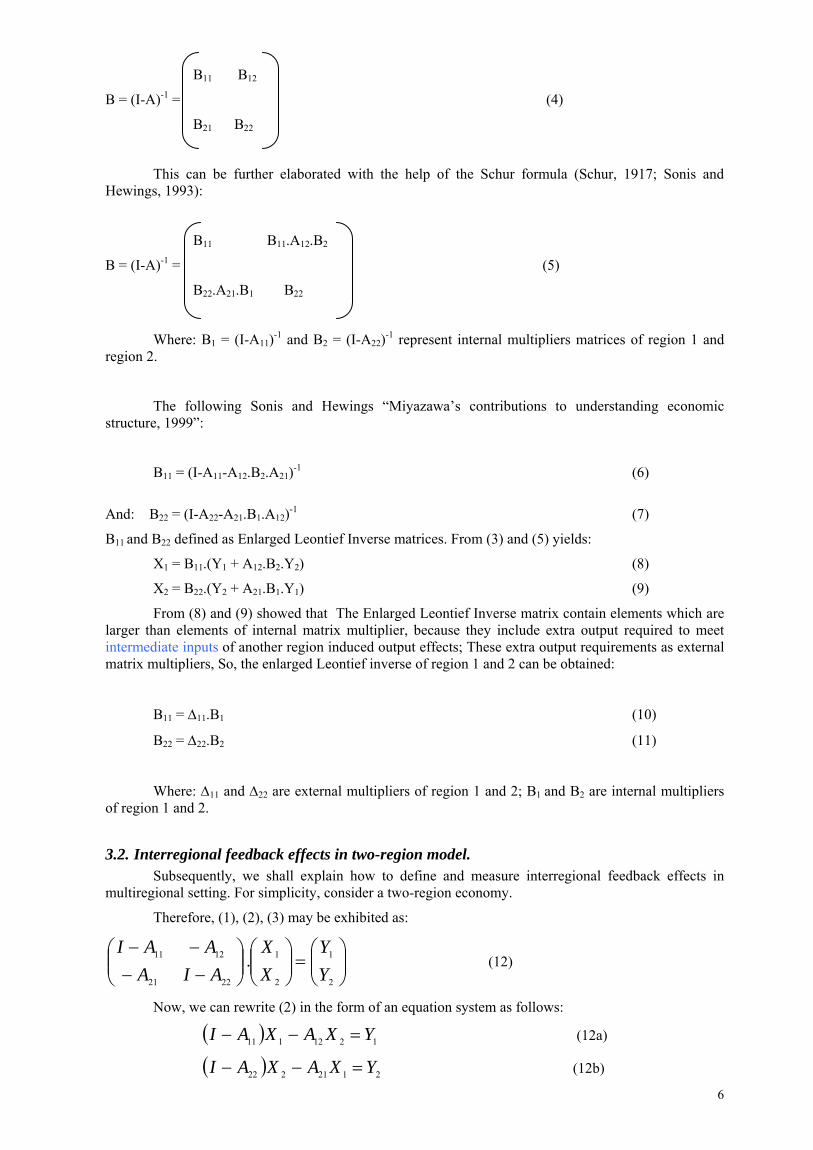
B11 B12

B = (I-A)-1 = (4)

B21 B22

6

This can be further elaborated with the help of the Schur formula (Schur, 1917; Sonis and Hewings, 1993):

B11 B11.A12.B2

B = (I-A)-1 = (5)

B22.A21.B1 B22

Where: B1 = (I-A11)-1 and B2 = (I-A22)-1 represent internal multipliers matrices of region 1 and region 2.

The following Sonis and Hewings “Miyazawa’s contributions to understanding economic structure, 1999”:

B11 = (I-A11-A12.B2.A21)-1 (6)

And: B22 = (I-A22-A21.B1.A12)-1 (7)

B11 and B22 defined as Enlarged Leontief Inverse matrices. From (3) and (5) yields:

X1 = B11.(Y1 + A12.B2.Y2) (8)

X2 = B22.(Y2 + A21.B1.Y1) (9)

From (8) and (9) showed that The Enlarged Leontief Inverse matrix contain elements which are larger than elements of internal matrix multiplier, because they include extra output required to meet intermediate inputs of another region induced output effects; These extra output requirements as external matrix multipliers, So, the enlarged Leontief inverse of region 1 and 2 can be obtained:

B11 = ∆11.B1 (10)

B22 = ∆22.B2 (11)

Where: ∆11 and ∆22 are external multipliers of region 1 and 2; B1 and B2 are internal multipliers of region 1 and 2.

3.2. Interregional feedback effects in two-region model.

Subsequently, we shall explain how to define and measure interregional feedback effects in multiregional setting. For simplicity, consider a two-region economy.

Therefore, (1), (2), (3) may be exhibited as:

⎟⎟⎠

⎞⎜⎜⎝

⎛−−−−

2221

1211

AIAAAI

⎟⎟⎠

⎞⎜⎜⎝

⎛=⎟⎟

⎠

⎞⎜⎜⎝

⎛

2

1

2

1.YY

XX

(12)

Now, we can rewrite (2) in the form of an equation system as follows:

( ) 1212111 YXAXAI =−− (12a)

( ) 2121222 YXAXAI =−− (12b)

Given a vector of changes in final demands in two regions, we can find the consequent changes in gross outputs in both regions. Assume, for simplicity, that Y2 = 0 (i.e. we are to assess the impacts on both regions of a change in final demand in region 1 only). Under these conditions, solving equations (2a) and (2b) for X1 and X2 may yield:

1211

222 ..)( XAAIX −−= (13)

2121

111 ..)( XAAIX −−= (14)

It can be observed that in eq. (4) is a measure of the total output multiplier or propagation effect of on , implying that in case of no change in region 1’s final demand, one unit increase in total output of region 2 may cause an increase in total output of region 1 by the amount of amount of .

121

11 )( AAI −−

2X 1X

121

11)( AAI −−

Similarly, is considered as the propagation effect of on , and has the analogous interpretation.

211

22 )( AAI −− 1X 2X

3.3. The Calculating Emission impacts based on interregional input output model.

The general economic input-output model system can be extended to encompass emissions from each sector. These consequences can only be estimated if the framework includes information on the environmental consequences of production within the various economic sectors, this is done by estimating a number of emission coefficients for each sectors indicating the amount of various substances emitting per output value.

The sectorial emission coefficients only relate to emission resulting directly from the production process. However, the production process also places an input demand on other sectors, thereby raising their production and emissions. The sum of these direct and indirect emissions can be calculated by Leontief – inverse matrix indicating for each sector the emission coefficients for the total direct and indirect environmental consequences.

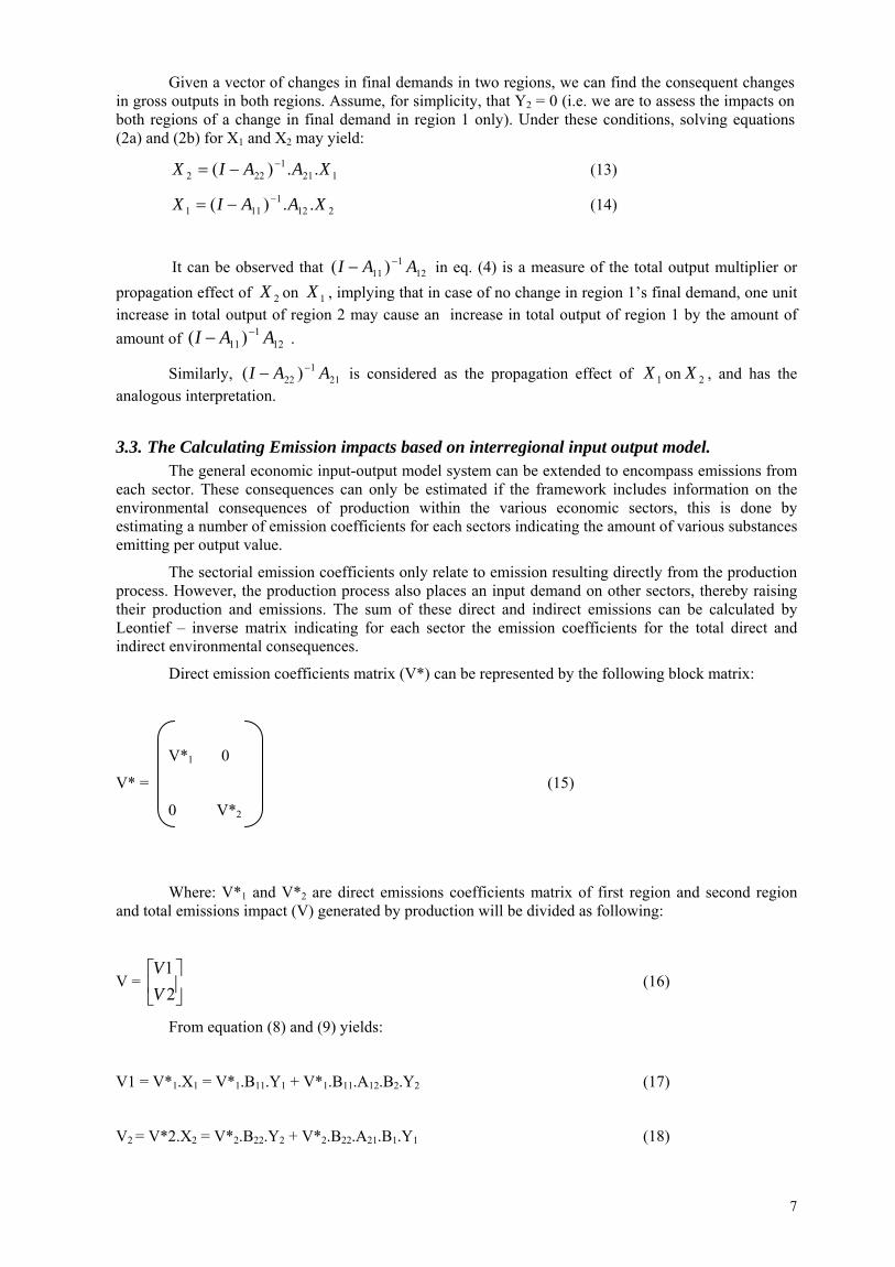
Direct emission coefficients matrix (V*) can be represented by the following block matrix:

V*1 0

V* = (15)

0 V*2

Where: V*1 and V*2 are direct emissions coefficients matrix of first region and second region and total emissions impact (V) generated by production will be divided as following:

V = (16) ⎥⎦

⎤⎢⎣

⎡21

VV

From equation (8) and (9) yields:

V1 = V*1.X1 = V*1.B11.Y1 + V*1.B11.A12.B2.Y2 (17)

V2 = V*2.X2 = V*2.B22.Y2 + V*2.B22.A21.B1.Y1 (18)

7

Using an explicit hierarchical order among the regions with this matrix decomposition technique, Sonis and Hewings (1993) identified the following multiplicative structure of Leontief inverse and Miyazawa partitioned multipliers:

∆11 0 I B1A12 B1 0 B = (I - A)-1

=

0 ∆22

. B2A21 I

. 0 B2

From (16), (17), (18), and (19) yield:

V = V*.B.Y (

Further, the matrix A is know as the direct requirements coefficients matrix and BLeontief inverse which frequently referred to as the total; requirement coefficients matrix. input – output model where only the productive sectors of the economy are assumed to be(determined by factors inside the productive system), all final demand are assumed to be dfactors outside the productive system. The model, however, can be closed with respect to hincluding in the matrix A one more column and row, for household consumption and respectively. This will form a new matrix denoted by C and (I-C)-1 is termed the closed inThis inverse matrix has one more column and row than the open matrix B, the last column inverse matrix is interpreted as the consumption multiplier ( the effect on the output of eachadditional unit of consumption) and last row as the income multiplier ( income created bysales of each sector).

The remaining rows and columns of the closed inverse (denoted by C*), the C8 conwhich are larger than those of the open inverse, because they include extra output requconsumption induced output effects, as a result of closed the model with respect to homatrix C* is also enlarged Leontief inverse type. Hence, the residual impacts generated band consumption can be estimated yield:

U = V*.C*.Y (21)

Where: U is total residual impact generated by production and consumption.

4. Empirical Study 4.1. On Economy

4.1.1. Overview of two – region system Prior to an analysis of unscheduled event, a brief digression will be made to explor

structure of the interregional system of Vietnam. In the empirical analysis using the equatifor calculating internal and external multipliers of HoChiMinh City (HCMC) and Rest(ROV) and equation (13), (14) for calculating interregional feedback effects of HCMC andapplied to a two – region between HCMC and rest of Vietnam (ROV) with 2000 interroutput table of Vietnam aggregated 12 sectors and some comparisons with result of 1996 input output table (this table compiled by private researcher group with financial assistanceNISSAN Study Foundation).

(19)

20)

is the open In an “open” endogenous etermined by ouseholds by value added, verse matrix. of the closed sector of an each unit of

tain elements ired to meet usehold. The y production

e the general ons (10),(11) of Vietnam ROV and a

egional input interregional provided by

8

9

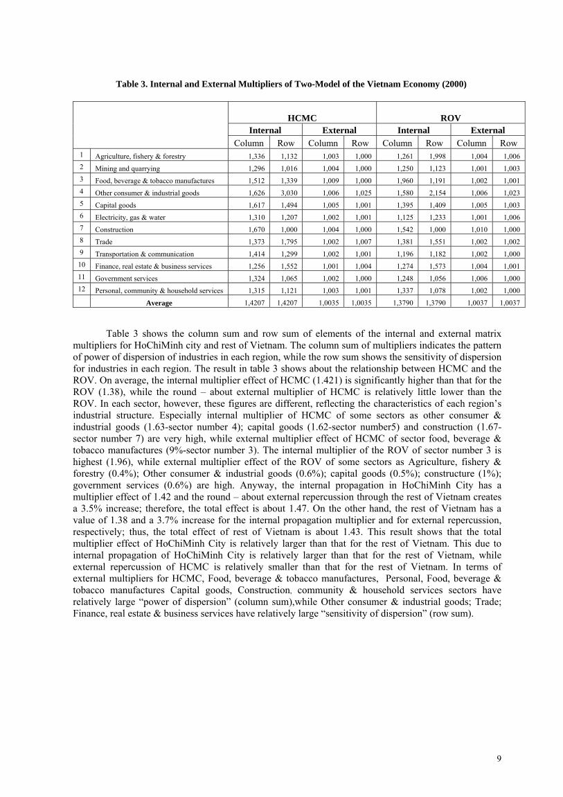
Table 3. Internal and External Multipliers of Two-Model of the Vietnam Economy (2000) HCMC ROV

Internal External Internal External

Column Row Column Row Column Row Column Row 1 Agriculture, fishery & forestry 1,336 1,132 1,003 1,000 1,261 1,998 1,004 1,006 2 Mining and quarrying 1,296 1,016 1,004 1,000 1,250 1,123 1,001 1,003 3 Food, beverage & tobacco manufactures 1,512 1,339 1,009 1,000 1,960 1,191 1,002 1,001 4 Other consumer & industrial goods 1,626 3,030 1,006 1,025 1,580 2,154 1,006 1,023 5 Capital goods 1,617 1,494 1,005 1,001 1,395 1,409 1,005 1,003 6 Electricity, gas & water 1,310 1,207 1,002 1,001 1,125 1,233 1,001 1,006 7 Construction 1,670 1,000 1,004 1,000 1,542 1,000 1,010 1,000 8 Trade 1,373 1,795 1,002 1,007 1,381 1,551 1,002 1,002 9 Transportation & communication 1,414 1,299 1,002 1,001 1,196 1,182 1,002 1,000 10 Finance, real estate & business services 1,256 1,552 1,001 1,004 1,274 1,573 1,004 1,001 11 Government services 1,324 1,065 1,002 1,000 1,248 1,056 1,006 1,000 12 Personal, community & household services 1,315 1,121 1,003 1,001 1,337 1,078 1,002 1,000 Average 1,4207 1,4207 1,0035 1,0035 1,3790 1,3790 1,0037 1,0037

Table 3 shows the column sum and row sum of elements of the internal and external matrix multipliers for HoChiMinh city and rest of Vietnam. The column sum of multipliers indicates the pattern of power of dispersion of industries in each region, while the row sum shows the sensitivity of dispersion for industries in each region. The result in table 3 shows about the relationship between HCMC and the ROV. On average, the internal multiplier effect of HCMC (1.421) is significantly higher than that for the ROV (1.38), while the round – about external multiplier of HCMC is relatively little lower than the ROV. In each sector, however, these figures are different, reflecting the characteristics of each region’s industrial structure. Especially internal multiplier of HCMC of some sectors as other consumer & industrial goods (1.63-sector number 4); capital goods (1.62-sector number5) and construction (1.67-sector number 7) are very high, while external multiplier effect of HCMC of sector food, beverage & tobacco manufactures (9%-sector number 3). The internal multiplier of the ROV of sector number 3 is highest (1.96), while external multiplier effect of the ROV of some sectors as Agriculture, fishery & forestry (0.4%); Other consumer & industrial goods (0.6%); capital goods (0.5%); constructure (1%); government services (0.6%) are high. Anyway, the internal propagation in HoChiMinh City has a multiplier effect of 1.42 and the round – about external repercussion through the rest of Vietnam creates a 3.5% increase; therefore, the total effect is about 1.47. On the other hand, the rest of Vietnam has a value of 1.38 and a 3.7% increase for the internal propagation multiplier and for external repercussion, respectively; thus, the total effect of rest of Vietnam is about 1.43. This result shows that the total multiplier effect of HoChiMinh City is relatively larger than that for the rest of Vietnam. This due to internal propagation of HoChiMinh City is relatively larger than that for the rest of Vietnam, while external repercussion of HCMC is relatively smaller than that for the rest of Vietnam. In terms of external multipliers for HCMC, Food, beverage & tobacco manufactures, Personal, Food, beverage & tobacco manufactures Capital goods, Construction, community & household services sectors have relatively large “power of dispersion” (column sum),while Other consumer & industrial goods; Trade; Finance, real estate & business services have relatively large “sensitivity of dispersion” (row sum).

10

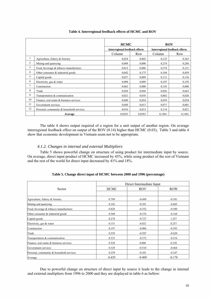
Table 4. Interregional feedback effects of HCMC and ROV

HCMC ROV

Interregional feedback effects Interregional feedback effects Column Row Column Row

1 Agriculture, fishery & forestry 0,024 0,002 0,125 0,363 2 Mining and quarrying 0,008 0,000 0,274 0,246 3 Food, beverage & tobacco manufactures 0,012 0,006 0,374 0,121 4 Other consumer & industrial goods 0,042 0,175 0,184 0,459 5 Capital goods 0,037 0,009 0,131 0,136 6 Electricity, gas & water 0,008 0,009 0,107 0,195 7 Construction 0,062 0,000 0,143 0,000 8 Trade 0,020 0,046 0,056 0,063 9 Transportation & communication 0,021 0,010 0,062 0,020 10 Finance, real estate & business services 0,040 0,054 0,039 0,054 11 Government services 0,049 0,013 0,071 0,001 12 Personal, community & household services 0,016 0,015 0,114 0,021

Average 0,0282 0,0282 0,1401 0,1401

The table 4 shows output required of a region for a unit output of another region. On average interregional feedback effect on output of the ROV (0.14) higher than HCMC (0.03), Table 3 and table 4 show that economic development in Vietnam seem not to be appropriate.

4.1.2. Changes in internal and external Multipliers

Table 5 shows powerful change on structure of using product for intermediate input by source. On average, direct input product of HCMC increased by 43%, while using product of the rest of Vietnam and the rest of the world for direct input decreased by 41% and 18%.

Table 5. Change direct input of HCMC between 2000 and 1996 (percentage) Direct Intermediate Input

Sector HCMC ROV ROW Agriculture, fishery & forestry 0.799 -0.499 -0.381

Mining and quarrying 0.142 -0.381 -0.685

Food, beverage & tobacco manufactures 0.828 -0.352 -0.580

Other consumer & industrial goods 0.560 -0.376 -0.164

Capital goods 0.278 -0.727 1.257

Electricity, gas & water 0.151 -0.821 0.257

Construction 0.197 -0.006 -0.393

Trade 0.559 -0.587 -0.620

Transportation & communication 0.533 -0.272 -0.516

Finance, real estate & business services 0.528 0.008 0.338

Government services 0.329 -0.510 -0.464

Personal, community & household services 0.239 -0.381 -0.187

Average 0.429 -0.409 -0.178

Due to powerful change on structure of direct input by source it leads to the change in internal and external multipliers from 1996 to 2000 and they are displayed in table 6 as bellow:

11

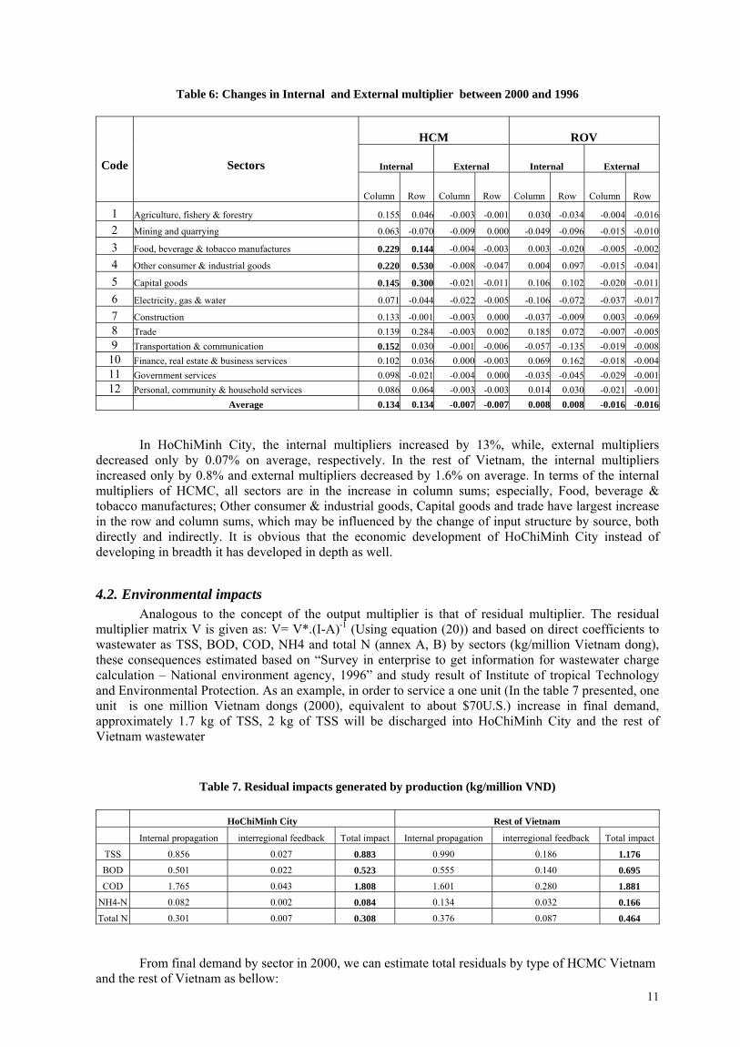
Table 6: Changes in Internal and External multiplier between 2000 and 1996

HCM ROV

Code Sectors Internal External Internal External

Column Row Column Row Column Row Column Row

1 Agriculture, fishery & forestry 0.155 0.046 -0.003 -0.001 0.030 -0.034 -0.004 -0.016

2 Mining and quarrying 0.063 -0.070 -0.009 0.000 -0.049 -0.096 -0.015 -0.010

3 Food, beverage & tobacco manufactures 0.229 0.144 -0.004 -0.003 0.003 -0.020 -0.005 -0.002

4 Other consumer & industrial goods 0.220 0.530 -0.008 -0.047 0.004 0.097 -0.015 -0.041

5 Capital goods 0.145 0.300 -0.021 -0.011 0.106 0.102 -0.020 -0.011

6 Electricity, gas & water 0.071 -0.044 -0.022 -0.005 -0.106 -0.072 -0.037 -0.017

7 Construction 0.133 -0.001 -0.003 0.000 -0.037 -0.009 0.003 -0.0698 Trade 0.139 0.284 -0.003 0.002 0.185 0.072 -0.007 -0.0059 Transportation & communication 0.152 0.030 -0.001 -0.006 -0.057 -0.135 -0.019 -0.008

10 Finance, real estate & business services 0.102 0.036 0.000 -0.003 0.069 0.162 -0.018 -0.00411 Government services 0.098 -0.021 -0.004 0.000 -0.035 -0.045 -0.029 -0.00112 Personal, community & household services 0.086 0.064 -0.003 -0.003 0.014 0.030 -0.021 -0.001

Average 0.134 0.134 -0.007 -0.007 0.008 0.008 -0.016 -0.016

In HoChiMinh City, the internal multipliers increased by 13%, while, external multipliers decreased only by 0.07% on average, respectively. In the rest of Vietnam, the internal multipliers increased only by 0.8% and external multipliers decreased by 1.6% on average. In terms of the internal multipliers of HCMC, all sectors are in the increase in column sums; especially, Food, beverage & tobacco manufactures; Other consumer & industrial goods, Capital goods and trade have largest increase in the row and column sums, which may be influenced by the change of input structure by source, both directly and indirectly. It is obvious that the economic development of HoChiMinh City instead of developing in breadth it has developed in depth as well.

4.2. Environmental impacts

Analogous to the concept of the output multiplier is that of residual multiplier. The residual multiplier matrix V is given as: V= V*.(I-A)-1 (Using equation (20)) and based on direct coefficients to wastewater as TSS, BOD, COD, NH4 and total N (annex A, B) by sectors (kg/million Vietnam dong), these consequences estimated based on “Survey in enterprise to get information for wastewater charge calculation – National environment agency, 1996” and study result of Institute of tropical Technology and Environmental Protection. As an example, in order to service a one unit (In the table 7 presented, one unit is one million Vietnam dongs (2000), equivalent to about $70U.S.) increase in final demand, approximately 1.7 kg of TSS, 2 kg of TSS will be discharged into HoChiMinh City and the rest of Vietnam wastewater

Table 7. Residual impacts generated by production (kg/million VND)

HoChiMinh City Rest of Vietnam

Internal propagation interregional feedback Total impact Internal propagation interregional feedback Total impact

TSS 0.856 0.027 0.883 0.990 0.186 1.176 BOD 0.501 0.022 0.523 0.555 0.140 0.695 COD 1.765 0.043 1.808 1.601 0.280 1.881

NH4-N 0.082 0.002 0.084 0.134 0.032 0.166 Total N 0.301 0.007 0.308 0.376 0.087 0.464

From final demand by sector in 2000, we can estimate total residuals by type of HCMC Vietnam and the rest of Vietnam as bellow:

12

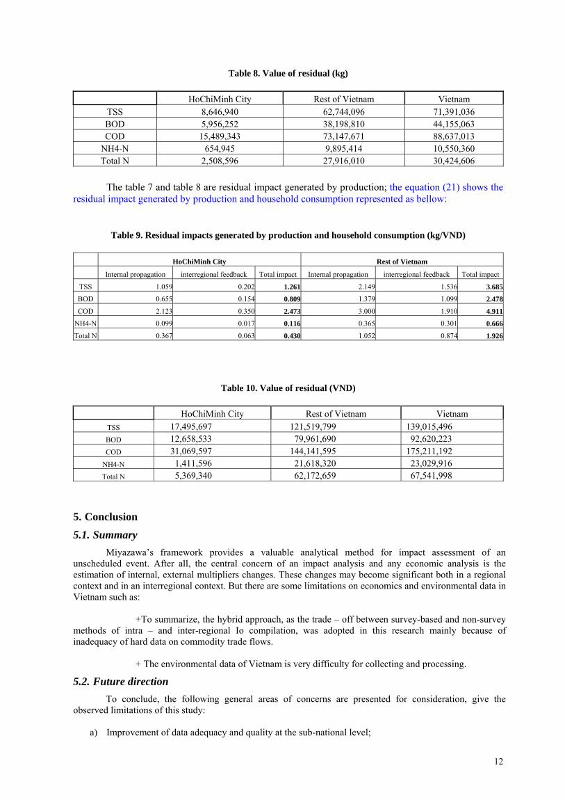
Table 8. Value of residual (kg)

HoChiMinh City Rest of Vietnam Vietnam TSS 8,646,940 62,744,096 71,391,036 BOD 5,956,252 38,198,810 44,155,063 COD 15,489,343 73,147,671 88,637,013

NH4-N 654,945 9,895,414 10,550,360 Total N 2,508,596 27,916,010 30,424,606

The table 7 and table 8 are residual impact generated by production; the equation (21) shows the residual impact generated by production and household consumption represented as bellow:

Table 9. Residual impacts generated by production and household consumption (kg/VND)

HoChiMinh City Rest of Vietnam

Internal propagation interregional feedback Total impact Internal propagation interregional feedback Total impact

TSS 1.059 0.202 1.261 2.149 1.536 3.685BOD 0.655 0.154 0.809 1.379 1.099 2.478COD 2.123 0.350 2.473 3.000 1.910 4.911

NH4-N 0.099 0.017 0.116 0.365 0.301 0.666Total N 0.367 0.063 0.430 1.052 0.874 1.926

Table 10. Value of residual (VND) HoChiMinh City Rest of Vietnam Vietnam

TSS 17,495,697 121,519,799 139,015,496 BOD 12,658,533 79,961,690 92,620,223 COD 31,069,597 144,141,595 175,211,192

NH4-N 1,411,596 21,618,320 23,029,916 Total N 5,369,340 62,172,659 67,541,998

5. Conclusion 5.1. Summary

Miyazawa’s framework provides a valuable analytical method for impact assessment of an unscheduled event. After all, the central concern of an impact analysis and any economic analysis is the estimation of internal, external multipliers changes. These changes may become significant both in a regional context and in an interregional context. But there are some limitations on economics and environmental data in Vietnam such as:

+To summarize, the hybrid approach, as the trade – off between survey-based and non-survey methods of intra – and inter-regional Io compilation, was adopted in this research mainly because of inadequacy of hard data on commodity trade flows.

+ The environmental data of Vietnam is very difficulty for collecting and processing.

5.2. Future direction To conclude, the following general areas of concerns are presented for consideration, give the observed limitations of this study:

a) Improvement of data adequacy and quality at the sub-national level;

13

b) Development and maintenance of framework for generation of commodity flow statistics useful in inter-regional Io compilation.

c) Enhancing scope and coverage of HCM IO compilation by taking into consideration such typical phenomena in urban economic as the contribution of the informal sector, environmental effects, the economic role of head office activities, etc.

d) Continuing efforts on IO based applied researches; CGE analysis, Miyazawa model, policy evaluation, etc.., give fiscal and technical resources and

e) Strengthening the country’s professional/technical capability in IO compilation and analysis

REFERENCES:

Akita, T., 1999, Environment and International Input-Output Analysis.

Akita, T., 1999, Trade and SO2 Emissions: An International Environmental Input-Output Analysis Between China and Japan.

Bui Trinh, 2001, Input-Output Model and its applications in economic and environmental analyzing and forecasting, HoChiMinh City Publisher.

Economic Institute of HoChiMinh, 1996 I-O Table for HCMC.

General Statistical Office of Vietnam, 1996 I-O Table of VietNam.

G.J.D. Hewings, M.Sonis, M. Madden. Y. Kimura editors, 1999 Understanding and Interpreting Economic Structure. Springer 1999

Institute of Tropical Techniques and Environmental Protection, 1998, Assessing environmental impacts of socio-economic development of HoChiMinh City, Bien Hoa and Vung Tau.

Kwan moon, K., Secretario, F. and Dakila, C.G., 2002, Structural Analysis of the Metro-Manila Economy based on Inter-Regional Input-Output Approach.

National environment Agency, 1996 “survey in enterprise to get information for wastewater”

Secretario, F., Kwan moon, K. and Dakila, C. G. 2002, The Metro-Manila Inter-Regional Input-Output Table: Its Attempt of Compilation By the Hybrid Approach.

S.M.N. Islam, 2002, Sustainability Science: Emerging Issues, Modeling, and Implication.

Sonis and Hewings, …. , Miyazawa’s contributions to Understanding Economic Structure.

South Asia Regional Committee for START and Netherlands Foundation for the Advancement of Tropical Research, 2000, Land-Ocean Interactions in the Coastal Zone, LOICZ Reports and Studies No 17.

14

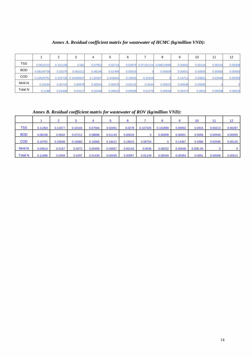
Annex A. Residual coefficient matrix for wastewater of HCMC (kg/million VND):

1 2 3 4 5 6 7 8 9 10 11 12

TSS 0.0810122 0.101106 0.081 0.07952 0.02714 0.02879 0.07101214 0.08510899 0.00002 0.00154 0.00243 0.00308

BOD 0.08106708 0.03276 0.061012 0.08196 0.01499 0.00019 0 0.00009 0.00001 0.00565 0.00565 0.00565

COD 0.10525752 0.102725 0.10405637 0.120307 0.240643 0.19615 0.10319 0 0.14711 0.03821 0.02046 0.05355

NH4-N 0.03194 0.00742 0.00978 0.00554 0.00078 0.00132 0.0044 0.00022 0.00048 0.00005 0 0

Total N 0.1186 0.01499 0.03127 0.02446 0.00623 0.00506 0.01275 0.00049 0.00374 0.0001 0.00008 0.00015

Annex B. Residual coefficient matrix for wastewater of ROV (kg/million VND):

1 2 3 4 5 6 7 8 9 10 11 12

TSS 0.11353 0.11877 0.10143 0.07564 0.02451 0.0278 0.107025 0.101899 0.00002 0.0015 0.00213 0.00297

BOD 0.08108 0.0634 0.07212 0.08686 0.01143 0.00019 0 0.00009 0.00001 0.0056 0.00549 0.00555

COD 0.10752 0.10648 0.10065 0.10065 0.18412 0.19615 0.09754 0 0.14457 0.0366 0.02046 0.05126

NH4-N 0.04514 0.0157 0.0072 0.00455 0.00057 0.00143 0.0036 0.00022 0.00046 5.00E-05 0 0

Total N 0.12486 0.0259 0.0297 0.01435 0.00435 0.00557 0.01149 0.00049 0.00354 0.0001 0.00008 0.00012