Inter-individual inequality in BMI: An analysis of Indonesian Family Life Surveys (1993–2007)

CitationVaezghasemi, Masoud, Fahad Razak, Nawi Ng, and S.V. Subramanian. 2016. “Inter-individual inequality in BMI: An analysis of Indonesian Family Life Surveys (1993–2007).” SSM - Population Health 2 (1): 876-888. doi:10.1016/j.ssmph.2016.09.013. http://dx.doi.org/10.1016/j.ssmph.2016.09.013.

Published Versiondoi:10.1016/j.ssmph.2016.09.013

Permanent linkhttp://nrs.harvard.edu/urn-3:HUL.InstRepos:34868718

Terms of UseThis article was downloaded from Harvard University’s DASH repository, and is made available under the terms and conditions applicable to Other Posted Material, as set forth at http://nrs.harvard.edu/urn-3:HUL.InstRepos:dash.current.terms-of-use#LAA

Share Your StoryThe Harvard community has made this article openly available.Please share how this access benefits you. Submit a story .

Accessibility

Contents lists available at ScienceDirect

SSM - Population Health

journal homepage: www.elsevier.com/locate/ssmph

Inter-individual inequality in BMI: An analysis of Indonesian Family LifeSurveys (1993–2007)

Masoud Vaezghasemia,b,⁎, Fahad Razakc,d,e,1, Nawi Nga, S.V. Subramanianf,1

a Epidemiology and Global Health Unit, Department of Public Health and Clinical Medicine, Umeå University, Umeå, Swedenb Umeå Centre for Gender Studies, Umeå University, Umeå, Swedenc Department of Medicine, University of Toronto, Toronto, Canadad Li Ka Shing Knowledge Institute and Division of General Internal Medicine, St. Michael’s Hospital, Toronto, Ontario, Canadae Harvard Center for Population and Development Studies, Cambridge, MA, USAf Department of Social and Behavioral Sciences, Harvard School of Public Health, Boston, MA, USA

A R T I C L E I N F O

Keywords:Body mass indexDistributional changeHealth inequalitiesObesitySocioeconomic statusIndonesian Family Life Survey

A B S T R A C T

Widening inequalities in mean Body Mass Index (BMI) between social and economic groups are welldocumented. However, whether changes in mean BMI are followed by changes in dispersion (or variance)and whether these inequalities are also occurring within social groups or across individuals remain under-studied. In addition, a substantial body of literature exists on the global increase in mean BMI and prevalence ofoverweight and obesity. However, whether this weight gain is shared proportionately across the whole spectrumof BMI distribution, also remains understudied. We examined changes in the distribution of BMI at thepopulation level over time to understand how changes in the dispersion reflect between-group compared towithin-group inequalities in weight gain. Moreover, we investigated the entire distribution of BMI to determinein which percentiles the most weight gain is occurring over time. Utilizing four waves (from 1993 to 2007) ofIndonesian Family Life Surveys (IFLS), we estimated changes in the mean and the variance of BMI over timeand across various socioeconomic groups based on education and households’ expenditure per capita in 53,648men and women aged 20–50 years. An increase in mean and standard deviation was observed among men (by4.3% and 25%, respectively) and women (by 7.3% and 20%, respectively) over time. Quantile-Quantile plotsshowed that higher percentiles had greater increases in BMI compared to the segment of the population at lowerpercentiles. While between socioeconomic group differences decreased over time, within-group differencesincreased and were more prominent among individuals with poor education and lower per capita expenditures.Population changes in BMI cannot be fully described by average trends or single parameters such as the meanBMI. Moreover, greater increases in within-group dispersion compared with between-group differences implythat growing inequalities are not merely driven by these socioeconomic factors at the population level.

1. Introduction

Rapid increases in the mean Body Mass Index (BMI) and theprevalence of overweight and obesity are widely documented in high-income countries, as well as low- to middle-income countries (LMICs)(Finucane et al., 2011; Jones-Smith, Gordon-Larsen, Siddiqi, &Popkin, 2011) including Indonesia (Roemling & Qaim, 2012; Usfar,Lebenthal, Atmarita Achadi, Soekirman, & Hadi, 2010). However,previous studies have predominantly relied on the change in mean orpoint estimates such as the prevalence of underweight, overweight and

obesity as a proxy for population level changes in BMI. A study usingDemographic Health Survey (DHS) data from 37 LMICs (excludingIndonesia) examined patterns of change across the entire distributionof BMI among women and revealed an increase in weight gain amonghigher BMI percentile groups suggesting that a single parameter, suchas mean BMI or percent overweight do not capture the divergence inthe degree of weight gain occurring across the population (Razak,Corsi, & Subramanian, 2013). However the DHS study was limited toa small number of repeated cross-sectional data and only to women.Therefore, further studies on both women and men in LMICs using

http://dx.doi.org/10.1016/j.ssmph.2016.09.013Received 24 February 2016; Received in revised form 12 September 2016; Accepted 30 September 2016

⁎ Corresponding author at: Epidemiology and Global Health Unit, Department of Public Health and Clinical Medicine, Umeå University, Umeå, Sweden.

1 Joint senior authors.E-mail address: masoud.vaezghasemi@umu.se (M. Vaezghasemi).

Abbreviations: BMI, Body Mass Index; IFLS, Indonesian Family Life Survey; LMICs, Low- and Middle-Income Countries; DHS, Demographic Health Survey; SD, Standard Deviation;QQ, Quantile-Quantile

SSM - Population Health 2 (2016) 876–888

2352-8273/ © 2016 The Authors. Published by Elsevier Ltd. This is an open access article under the CC BY-NC-ND license (http://creativecommons.org/licenses/BY-NC-ND/4.0/).

MARK

longitudinal datasets or datasets with a greater number of study cycleswas suggested to provide deeper insight into the varying patterns ofweight gain over time (Razak et al., 2013).

Previous studies in Indonesia have shown increases in the pre-valence of overweight and obesity as children grow to adolescents(Julia, van Weissenbruch, Prawirohartono, Surjono, & Delemarre-vande Waal, 2008) or significant increases in body weight and mean BMIamong women of productive age (Winkvist, Nurdiati, Stenlund, &Hakimi, 2000). A recent study on obesity trend and its determinantshas likewise shown a pronounced rise in overweight among women, inrural areas, and among low income individuals of the populationcompared to men, urban areas and high income individuals, whileunderweight still persists in Indonesia (Roemling & Qaim, 2012). Inaddition, households' inequalities in dual burden of malnutrition –

coexistence of both under- and overweight in the same household –were also examined between socioeconomic groups and residentialenvironments reporting rising intra-household inequalities and be-tween socioeconomic group differences (Roemling & Qaim, 2013;Vaezghasemi et al., 2014; Hanandita & Tampubolon, 2015). Theseprior papers that have focused on social group differences in health arenecessary for targeting investments to the worst off groups and agroup-level approach can support the creation of laws and programsthat seek to eliminate social group differences. For example, we mightask how mean BMI of the poor compares to that of the rich. Moreover,the WHO recommends that health indicators should be reported bygroups, or “equity stratifiers” for the purposes of monitoring healthinequities (Zheng et al., 2011).

However, few studies have examined whether inequalities in weightgain are occurring within social groups or specific segments of thepopulation, which is a measure of inter-individual inequalities ratherthan between-group inequalities (Krishna, Razak, Lebel, Smith, &Subramanian, 2015). In this study, we utilized standard deviation (SD)and variance in BMI as measures of inequality to assess the population-level dispersion across individuals within groups. The theoreticalframework of our study is based on what Murray and Gakidou definedas “health inequality”, which is variation in health status acrossindividuals in a population (Gakidou, Murray, & Frenk, 2000;Murray, Gakidou & Frenk, 1999). To study health inequalities, theyproposed two complementary approaches: (i) measuring social groupinequalities by differences in mean values or the prevalence of healthoutcomes between social groups and (ii) measuring individual inequal-ities by differences between individuals and within groups (Gakidouet al., 2000; Murray et al., 1999). Although less often considered in theepidemiologic literature, variations between individuals may providecritical information as the same average level of health could corre-spond to substantial variation across individuals in that population(Murray et al., 1999).

Indonesia is the fourth most populous country in the world and oneof Southeast Asia’s highly performing economies which has beenexperiencing striking social and economical changes during the lasttwo decades. To the best of our knowledge, no study in Indonesia has

previously addressed (i) changes in the distribution of BMI acrossvarious percentiles of the population and (ii) within-group or inter-individual inequalities in the distribution of BMI over time.

2. Subjects and methods

2.1. Data source

We utilized a nationally representative data from an on-goinglongitudinal socioeconomic and health survey, called the IndonesianFamily Life Survey (IFLS) (http://www.rand.org/labor/FLS/IFLS.html). The IFLS employed a multi-stage stratified systematicsampling design based on the stratification of provinces and urban/rural locations. In the first wave (1993) thirteen of twenty-sevenprovinces, representing 83% of the population were selected. TheIFLS consists of four waves of data collected in 1993, 1997–98,2000, and 2007–08. Our analyses were mainly performed on thecross-sectional data from these waves. Relatively few large-scalelongitudinal surveys are available for LMICs. IFLS is the only large-scale longitudinal survey available for Indonesia. Because data areavailable for the same individuals from multiple points in time, IFLSaffords an opportunity to understand the dynamics of behavior at theindividual, household and family, and community levels (Strauss,Witoelar, Sikoki, & Wattie, 2009).

2.2. Study subjects

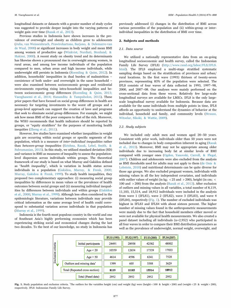
We included only adult men and women aged 20–50 years.Consistent with prior work, individuals older than 50 years were notincluded due to changes in body composition inherent in aging (Razaket al., 2013). Moreover, BMI may not be appropriate among olderindividuals due to increasing body fat at similar levels of BMIcompared with younger ones (Ogden, Yanovski, Carroll, & Flegal,2007). Children and adolescents were also excluded from the analysisas BMI thresholds used for adults may not apply to them (de Onis &Lobstein, 2010) and nutritional determinants can be quite diverse forthose age groups. We also excluded pregnant women, individuals withmissing values in all the key independent covariates, and individualswith outlier values of weight (in kg; < 25 and > 200), height (in cm; <100 and > 200) from the analysis (Razak et al., 2013). After exclusionof outliers and missing values in all variables, a total number of 8,119,11,103, 15,514, and 18,912 individuals were included in the analysisfrom wave 1 (IFLS1), wave 2 (IFLS2), wave 3 (IFLS3), and wave 4(IFLS4), respectively (Fig. 1). The number of excluded individuals washighest in IFLS3 and IFLS4 with about sixteen percent. The highernumber of missing values found in the anthropometric measurementswere mainly due to the fact that household members either moved orwere not available for physical health measurements. We also created apanel dataset including all individuals (n=2,952) who participated inall four waves in order to compare their BMI distribution parameters aswell as the prevalence of underweight, normal weight, overweight, and

Fig. 1. Study population and exclusion criteria. *The outliers for the variables height (cm) and weight (kg) were (height < 100 & height > 200) and (weight < 25 & weight > 200),respectively. IFLS: Indonesian Family Life Survey.

M. Vaezghasemi et al. SSM - Population Health 2 (2016) 876–888

877

obesity with those observed in the repeated cross-sectional data.

2.3. Outcome variable

The outcome of interest was BMI measured as a ratio of weight (kg)to the square of height (m). BMI is considered by the WHO to be astandard and useful population measure of weight status used in large-scale surveys of nutritional status in adults (WHO, 1995). It is aninexpensive and easy-to-perform method of screening for weightcategories at the population level, for example underweight, normalor healthy weight, overweight, and obesity. The definition of normalweight is BMI 18.5–24.99, based on WHO (World HealthOrganization, 2000), whereas a BMI 18.5–23, may be more appro-priate for Asians (Deurenberg, Deurenberg-Yap, & Guricci, 2002;WHO Expert Consultation, 2004). Two specially trained nurses re-corded physical measurements, including height and weight on allhousehold members (Strauss et al., 2009).

2.4. Covariates

The covariates were (i) gender (men and women), (ii) age (20–50years), (iii) occupation (never worked and worked), (iv) education (noschooling, elementary, secondary, and university), (v) household'sliving standard presented as quartiles of per capita expenditure (withthe first quartile being considered as “lowest per capita expenditure”),and (vi) place of residence (urban and rural). Household per capitaexpenditure (total household expenditure divided by number of house-hold members) was used as a proxy for a household's living standardand contained information about households' food expenditures andnon-food consumption during one month measured in IndonesianRupiah (Strauss et al., 2009).

2.5. Analysis

2.5.1. Distributional parameters of BMIBMI was age-adjusted prior to analysis. Age adjustment was

achieved by regressing BMI on age and quadratic age, followed bythe addition of the grand mean to the residuals from this model. Weused age-adjusted BMI for both repeated cross-sectional and paneldata to present and compare the distributional parameters over time:mean, SD, 5th, 50th, and 95th percentiles for all individuals (men andwomen separately) and for each study wave. We used both cross-sectional and panel data to compare the distributional parameter ofBMI. For the rest of the analysis only repeated cross-sectional datawere used. We calculated the percent change for all parameters in wave1 (1993) to wave 4 (2007).

2.5.2. Graphical analysis of patterns of BMI distributional changesAge-adjusted BMI was also used for the graphical analysis. There is

no standard approach to graphically examining distributional changesin BMI (Flegal & Troiano, 2000). As demonstrated previously (Razaket al., 2013; Krishna et al., 2015) Quantile-Quantile (QQ) plots canprovide useful information about changes in BMI distribution (Wilk &Gnanadesikan, 1968). Using this approach, we plotted percentiles ofBMI at the recent study cycles (wave 2, wave 3, and wave 4) againstpercentiles of BMI from the baseline study cycle (wave 1). If the twodistributions being compared were exactly the same, the points in theQQ plot would lie on the line y=x, and points above the equality line(y=x) represent a higher level of BMI in subsequent study waves. QQplots are particularly suitable for detecting the increasing distance fromthe line of equality at the tails of the distribution (Wilk &Gnanadesikan, 1968).

2.5.3. Between-group and within-group differences of BMI mean andvariance

We computed the mean and variance of BMI for each category of

education, and for each quartile of per capita expenditure for men andwomen separately for each study wave. Absolute and relative differ-ences in group mean BMI were calculated between the highest andlowest education level and the highest and lowest per capita expendi-tures. In addition, whithin-group differences (i.e. between individualdifferences) were calculated based on the percent change in SD andvariance from IFLS1 to IFLS4. We applied mean comparison test (t-test) and variance comparison test (sdtest) and reported p-values for allthe percentage changes in the analysis. P-values for percentage changesin absolute and relative differences was calculated by regressing BMIon the interaction between time (IFLS1 and IFLS4) and education orper capita expenditure.

2.5.4. Variance differences in regression modelsWe ran several univariate regressions on BMI and each covariate

(one at a time) for men and women separately for IFLS1 and IFLS4. Wedid this to observe how much of the variation is explained by eachcovariate separately compared with the null model (empty modelreporting total variance around the global mean BMI), and how itwas changing over time. In addition, for each study wave, we ranseveral different ordinary least squares regression models by regressingBMI on (i) age and gender (Model I); (ii) age, gender, and occupation(Model II); (iii) age, gender, occupation, education and per capitaexpenditure (Model III); and (iv) age, gender, occupation, education,per capita expenditure, and place of residence (Model IV). We onlypresented the variance to illustrate variability in the distribution ofBMI over the study waves after accounting for the socioeconomicfactors. We presented percent change in variance between Model I andModel IV to show the extent to which the variation in BMI is explainedby these socioeconomic factors, and between wave 1 and wave 4 toshow how population level variance was changing over time. Forinstance, we subtracted the variance in model I by the variance inmodel IV. We later divided this by the variance in model I andmultiplied it by 100 (Merlo et al., 2006). This gives us the percentageof the variance attenuated or explained by inclusion of all the socio-economic factors for each study wave. STATA software version 13.1was used for analysis in this study (StataCorp. 2013. Stata: Release 13.Statistical Software. College Station, TX: StataCorp LP).

3. Results

3.1. General characteristics of the study population

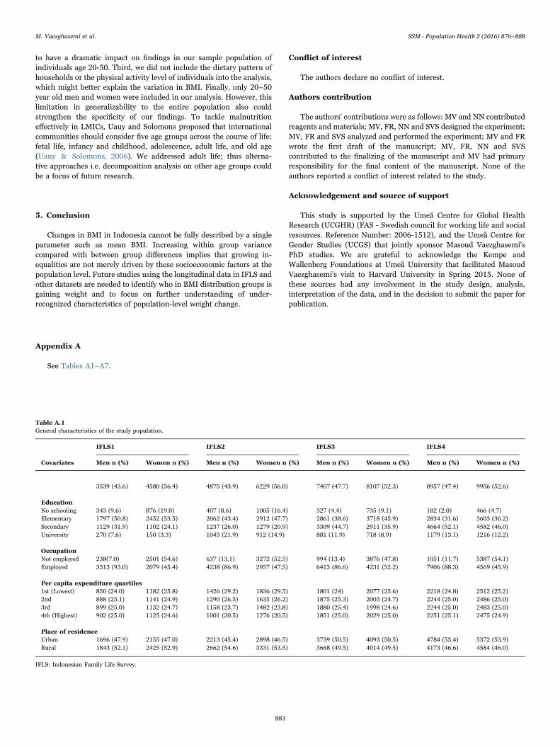
Table A.1 presents descriptive statistics (numbers and percentages)about the IFLS from 1993–2007. In IFLS1 9.6% of men and 19% ofwomen had no schooling. The percentage with no schooling decreasedto 2% for men and 4.7% for women in IFLS4. In IFLS4 almost the samepercentage of men (13.1%) and women (12.2%) had university educa-tion. Approximately 90% of men and 50% of women reported beingemployed across all the study waves. The proportion of men andwomen who lived in urban area increased from 47.9% in IFLS1 to53.4% in IFLS4 and from 47.0% to 53.9%, respectively.

3.2. Distributional parameters of BMI

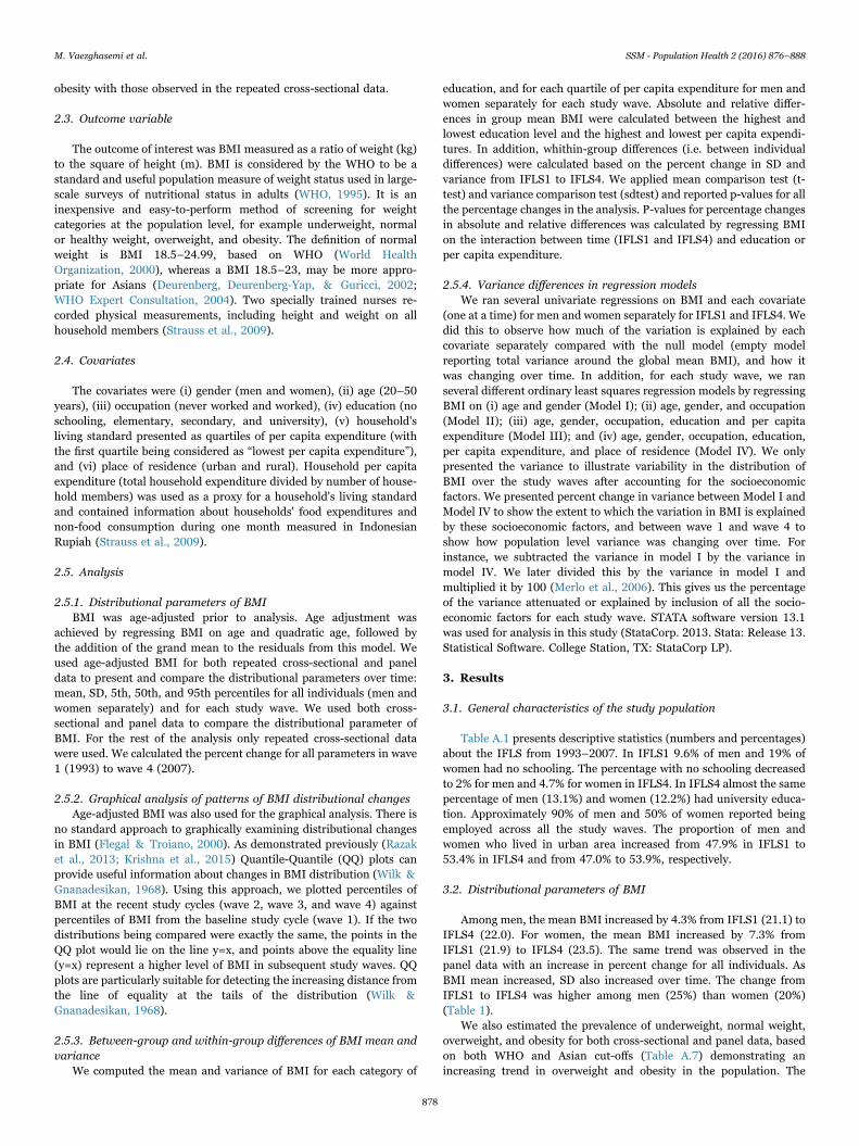
Among men, the mean BMI increased by 4.3% from IFLS1 (21.1) toIFLS4 (22.0). For women, the mean BMI increased by 7.3% fromIFLS1 (21.9) to IFLS4 (23.5). The same trend was observed in thepanel data with an increase in percent change for all individuals. AsBMI mean increased, SD also increased over time. The change fromIFLS1 to IFLS4 was higher among men (25%) than women (20%)(Table 1).

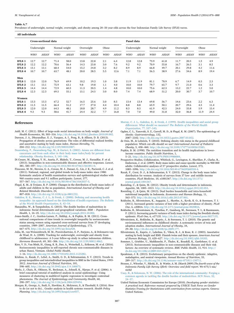
We also estimated the prevalence of underweight, normal weight,overweight, and obesity for both cross-sectional and panel data, basedon both WHO and Asian cut-offs (Table A.7) demonstrating anincreasing trend in overweight and obesity in the population. The

M. Vaezghasemi et al. SSM - Population Health 2 (2016) 876–888

878

results from the last cross-sectional data, based on the Asian cut-offillustrates that 41.1% of all individuals are overweight (28.5%) or obese(12.6%), while 10.7% are underweight.

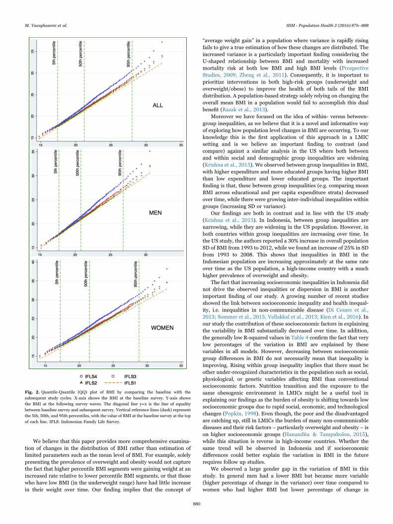
3.3. Patterns of BMI distribution change over time

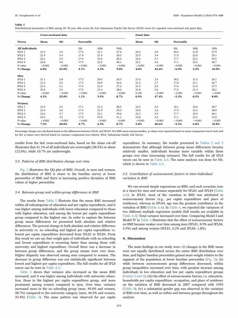
Fig. 2 illustrates the QQ plot of BMI. Overall, in men and women,the distribution of BMI is closer to the baseline survey at lowerpercentiles of BMI and there is increasing positive deviation of BMIvalues at higher percentiles.

3.4. Between-group and within-group differences in BMI

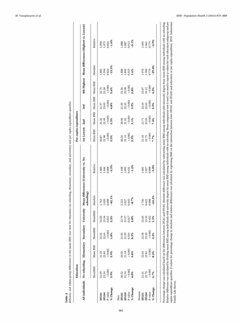
The results from Table 2 illustrate that the mean BMI increasedwithin all subcategories of education and per capita expenditure, and itwas higher among individuals with lower education compared to thosewith higher education, and among the lowest per capita expendituregroup compared to the highest one. In order to capture the betweengroup mean differences we presented both absolute and relativedifferences. The percent change in both absolute and relative differencein university vs. no schooling and highest per capita expenditure vs.lowest per capita expenditure decreased from IFLS1 to IFLS4. Fromthis result we can say that weight gain of individuals with no schoolingand lowest expenditure is occurring faster than among those withuniversity and highest expenditure. Overall there was a decrease inbetween group differences, and the group means were very close.Higher disparity was observed among men compared to women. Thedecrease in group difference was not statistically significant betweenlowest and highest per capita expenditure. The full results for all IFLSwaves can be seen in Table A.2.

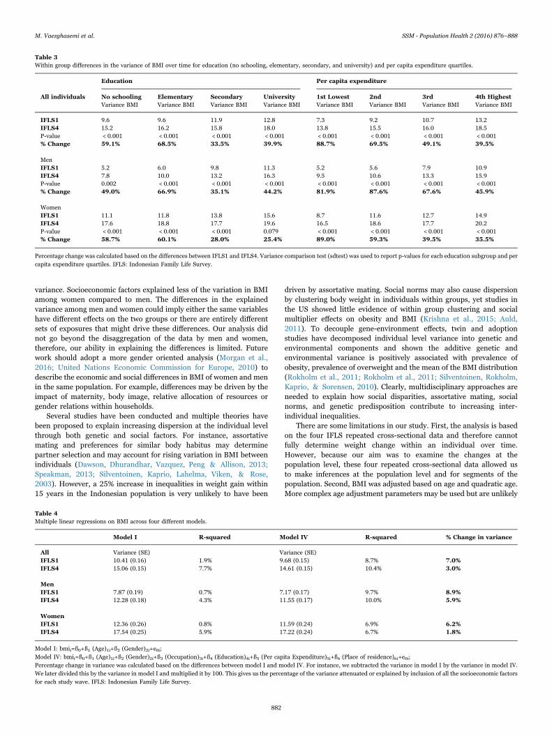
Table 3 shows that variance also increased as the mean BMIincreased, and it was higher among individuals with university educa-tion, those in the highest per capita expenditure group, and moreprominent among women compared to men. Over time, varianceincreased more in the no schooling group (men, 49.0% and women,58.7%) compared to the university category (men, 44.2% and women,25.4%) (Table 3). The same pattern was observed for per capita

expenditure. In summary, the results presented in Tables 2 and 3demonstrate that although between group mean differences becamerelatively smaller, individuals became more variable within thesegroups over time (increasing variance). The full results for all IFLSwaves can be seen in Table A.4. The same analysis was done for SD,which is shown in Table A.3.

3.5. Contribution of socioeconomic factors in inter-individualvariation in BMI

We ran several simple regressions on BMI, and each covariate (oneat a time) for men and women separately for IFLS1 and IFLS4 (TableA.6). In IFLS1, most of the variation in BMI was attributed tosocioeconomic factors (e.g., per capita expenditure and place ofresidence), whereas in IFLS4, age was the greatest contributor in thevariation of BMI (Table A.6). In Table 4, we reported the variances oftwo different multiple regression models (full results are available inTable A.5). Total variance increased over time. Comparing Model I andModel IV in Table 4 illustrates that the effect of socioeconomic factorson BMI became weaker over time among men (IFLS1, 8.9% and IFLS4,5.9%) and among women (IFLS1, 6.2% and IFLS4, 1.8%).

4. Discussion

The main findings in our study were: (i) changes in the BMI meanwere not equally distributed across the entire BMI distribution overtime, and higher baseline percentiles gained more weight relative to thesegment of the population at lower baseline percentiles (Fig. 2); (ii)while between socioeconomic group differences decreased, withingroup inequalities increased over time, with greatest increase amongindividuals in low education and low per capita expenditure groups(Tables 2 and 3); (iii) the effect of socioeconomic factors, i.e. education,households per capita expenditure, occupation, and place of residencyon the variation of BMI decreased in 2007 compared with 1993(Table 4); (iv) a substantial gender gap was observed in the variationof BMI over time, as well as within and between groups throughout theanalysis.

Table 1Distributional parameters of BMI among 20–50 year olds across the four Indonesian Family Life Survey (IFLS) waves for repeated cross-sectional and panel data.

Cross-sectional data Panel data

Waves Mean SD Percentile Mean SD Percentile

All individuals 5th 50th 95th 5th 50th 95thIFLS 1 21.5 3.2 17.2 21.1 27.6 22.2 3.0 18.2 21.8 27.9IFLS 2 21.9 3.4 17.4 21.4 28.2 22.5 3.4 17.9 22.0 29.1IFLS 3 22.1 3.5 17.4 21.6 28.6 22.6 3.7 17.7 22.2 29.5IFLS 4 22.8 4.0 17.9 22.2 30.1 23.1 4.3 17.1 22.5 30.7P-value < 0.001 < 0.001 < 0.001 < 0.001 < 0.001 < 0.001 < 0.001 < 0.001 < 0.001 < 0.001% Change 6.0% 25.0% 4.1% 5.2% 9.0% 4.0% 42.4% −6.0% 3.2% 10.0%

MenIFLS 1 21.1 2.8 17.3 20.6 26.3 21.6 2.4 18.2 21.3 26.1IFLS 2 21.3 2.9 17.4 20.9 26.6 21.5 2.7 17.8 21.1 26.7IFLS 3 21.5 3.1 17.4 21.0 27.2 21.5 2.9 17.6 21.0 27.3IFLS 4 22.0 3.5 17.5 21.4 28.6 21.8 3.6 17.2 21.4 28.2P-value < 0.001 < 0.001 < 0.001 < 0.001 < 0.001 0.102 < 0.001 < 0.001 < 0.001 < 0.001% Change 4.3% 25.0% 1.1% 3.9% 8.7% 0.9% 47.4% −5.5% 0.5% 8.0%

WomenIFLS 1 21.9 3.5 17.1 21.5 28.5 22.5 3.2 18.1 22.0 28.7IFLS 2 22.4 3.6 17.4 21.9 29.3 23.0 3.6 17.9 22.5 30.0IFLS 3 22.6 3.7 17.5 22.1 29.6 23.2 3.9 17.7 22.9 30.1IFLS 4 23.5 4.2 17.9 22.9 31.1 23.8 4.5 17.1 23.5 31.8P-value < 0.001 < 0.001 < 0.001 < 0.001 < 0.001 < 0.001 < 0.001 < 0.001 < 0.001 < 0.001% Change 7.3% 20.0% 4.7% 6.5% 8.7% 5.8% 40.6% −5.5% 6.8% 10.8%

Percentage change was calculated based on the differences between IFLS1 and IFLS4. For BMI mean and percentiles, p-values were reported based on mean comparison test (t-test) andfor SD, p-values were derived based on variance comparison test (sdtest). IFLS: Indonesian Family Life Survey.

M. Vaezghasemi et al. SSM - Population Health 2 (2016) 876–888

879

We believe that this paper provides more comprehensive examina-tion of changes in the distribution of BMI rather than estimation oflimited parameters such as the mean level of BMI. For example, solelypresenting the prevalence of overweight and obesity would not capturethe fact that higher percentile BMI segments were gaining weight at anincreased rate relative to lower percentile BMI segments, or that thosewho have low BMI (in the underweight range) have had little increasein their weight over time. Our finding implies that the concept of

“average weight gain” in a population where variance is rapidly risingfails to give a true estimation of how these changes are distributed. Theincreased variance is a particularly important finding considering theU-shaped relationship between BMI and mortality with increasedmortality risk at both low BMI and high BMI levels (ProspectiveStudies, 2009; Zheng et al., 2011). Consequently, it is important toprioritize interventions in both high-risk groups (underweight andoverweight/obese) to improve the health of both tails of the BMIdistribution. A population-based strategy solely relying on changing theoverall mean BMI in a population would fail to accomplish this dualbenefit (Razak et al., 2013).

Moreover we have focused on the idea of within- versus between-group inequalities, as we believe that it is a novel and informative wayof exploring how population level changes in BMI are occurring. To ourknowledge this is the first application of this approach in a LMICsetting and is we believe an important finding to contrast (andcompare) against a similar analysis in the US where both betweenand within social and demographic group inequalities are widening(Krishna et al., 2015). We observed between group inequalities in BMI,with higher expenditure and more educated groups having higher BMIthan low expenditure and lower educated groups. The importantfinding is that, these between group inequalities (e.g. comparing meanBMI across educational and per capita expenditure strata) decreasedover time, while there were growing inter-individual inequalities withingroups (increasing SD or variance).

Our findings are both in contrast and in line with the US study(Krishna et al., 2015). In Indonesia, between group inequalities arenarrowing, while they are widening in the US population. However, inboth countries within group inequalities are increasing over time. Inthe US study, the authors reported a 30% increase in overall populationSD of BMI from 1993 to 2012, while we found an increase of 25% in SDfrom 1993 to 2008. This shows that inequalities in BMI in theIndonesian population are increasing approximately at the same rateover time as the US population, a high-income country with a muchhigher prevalence of overweight and obesity.

The fact that increasing socioeconomic inequalities in Indonesia didnot drive the observed inequalities or dispersion in BMI is anotherimportant finding of our study. A growing number of recent studiesshowed the link between socioeconomic inequality and health inequal-ity, i.e. inequalities in non-communicable disease (Di Cesare et al.,2013; Sommer et al., 2015; Vellakkal et al., 2013; Kien et al., 2016). Inour study the contribution of these socioeconomic factors in explainingthe variability in BMI substantially decreased over time. In addition,the generally low R-squared values in Table 4 confirm the fact that verylow percentages of the variation in BMI are explained by thesevariables in all models. However, decreasing between socioeconomicgroup differences in BMI do not necessarily mean that inequality isimproving. Rising within group inequality implies that there must beother under-recognized characteristics in the population such as social,physiological, or genetic variables affecting BMI than conventionalsocioeconomic factors. Nutrition transition and the exposure to thesame obesogenic environment in LMICs might be a useful tool inexplaining our findings as the burden of obesity is shifting towards lowsocioeconomic groups due to rapid social, economic, and technologicalchanges (Popkin, 1998). Even though, the poor and the disadvantagedare catching up, still in LMICs the burden of many non-communicablediseases and their risk factors – particularly overweight and obesity – ison higher socioeconomic groups (Hanandita & Tampubolon, 2015),while this situation is reverse in high-income countries. Whether thesame trend will be observed in Indonesia and if socioeconomicdifferences could better explain the variation in BMI in the futurerequires follow up studies.

We observed a large gender gap in the variation of BMI in thisstudy. In general men had a lower BMI but became more variable(higher percentage of change in the variance) over time compared towomen who had higher BMI but lower percentage of change in

Fig. 2. Quantile-Quantile (QQ) plot of BMI by comparing the baseline with thesubsequent study cycles. X-axis shows the BMI at the baseline survey. Y-axis showsthe BMI at the following survey waves. The diagonal line y=x is the line of equalitybetween baseline survey and subsequent survey. Vertical reference lines (dash) representthe 5th, 50th, and 95th percentiles, with the value of BMI at the baseline survey at the topof each line. IFLS: Indonesian Family Life Survey.

M. Vaezghasemi et al. SSM - Population Health 2 (2016) 876–888

880

Table

2Between-an

dwithin-groupdifferencesin

themeanBMIov

ertimefored

ucation

(noschoo

ling,

elem

entary,secondary,

anduniversity)an

dper

capitaexpen

diture

quartiles.

Educa

tion

Perca

pitaexpenditure

All

individ

uals

Nosc

hooling

Elem

entary

Seco

ndary

Univers

ity

Mean

diff

ere

nce

s(U

nivers

ityvs.

No

schooling)

1st

Lowest

2nd

3rd

4th

Highest

Meandiff

ere

nce

s(H

ighest

vs.

Lowest)

MeanBMI

MeanBMI

MeanBMI

MeanBMI

Absolute

Relative

MeanBMI

MeanBMI

MeanBMI

MeanBMI

Absolute

Relative

IFLS1

21.09

21.55

22.25

22.85

1.76

21.08

420

.87

21.36

21.97

22.75

1.88

31.09

0IF

LS4

22.34

22.81

22.64

23.36

1.02

01.04

621

.98

22.49

23.03

23.58

1.59

41.07

3P-value

<0.00

1<0.00

1<0.00

10.02

10.00

80.00

8<0.00

1<0.00

1<0.00

1<0.00

10.82

40.82

4%

Change

5.9%

5.9%

1.8%

2.2%

−42.1%

−3.5%

5.3%

5.3%

4.8%

3.6%

−15.3%

−1.6%

Men

IFLS1

20.52

20.92

21.92

22.74

2.22

11.10

820

.55

20.90

21.50

22.36

1.80

81.08

8IF

LS4

21.34

21.54

21.99

23.37

2.02

71.09

521

.14

21.55

22.35

22.98

1.84

21.08

7P-value

<0.00

1<0.00

10.55

40.01

70.63

50.63

5<0.00

1<0.00

1<0.00

1<0.00

10.91

30.91

3%

Change

4.0%

3.0%

0.3%

2.8%

−8.7%

−1.2%

2.9%

3.1%

3.9%

2.8%

1.6%

−0.1%

Wom

enIF

LS1

21.31

22.01

22.58

23.05

1.73

61.08

121

.10

21.71

22.34

23.07

1.97

01.09

3IF

LS4

22.73

23.81

23.30

23.35

0.62

21.02

722

.73

23.33

23.65

24.12

1.39

01.06

1P-value

<0.00

1<0.00

1<0.00

10.42

20.00

80.00

8<0.00

1<0.00

1<0.00

1<0.00

10.77

40.77

4%

Change

6.7%

8.2%

3.2%

1.3%

−64.2%

−5.0%

7.7%

7.4%

5.9%

4.5%

−29.4%

−2.9%

Percentage

chan

gewas

calculatedba

sedon

thedifferencesbe

tweenIFLS1

andIFLS4

.Absolute

difference

was

calculatedby

subtractingmeanBMIam

ongindividualswithuniversity

degreefrom

meanBMIam

ongindividualswithnoschoo

ling.

Relativedifference

was

calculatedby

dividingmeanBMIam

ongindividualswithuniversity

degreeby

meanBMIam

ongindividualswithnoschoo

ling.

Meancomparison

test

(t-test)was

usedto

reportp-values

foreach

education

subg

roupan

dper

capitaexpen

diture

quartiles.

P-values

forpercentage

chan

gein

absolute

andrelative

differenceswas

calculatedby

regressingBMIon

theinteractionbe

tweentime(IFLS1

andIFLS4

)an

ded

ucation

orper

capitaexpen

diture.IFLS:

Indon

esian

Fam

ilyLifeSu

rvey.

M. Vaezghasemi et al. SSM - Population Health 2 (2016) 876–888

881

variance. Socioeconomic factors explained less of the variation in BMIamong women compared to men. The differences in the explainedvariance among men and women could imply either the same variableshave different effects on the two groups or there are entirely differentsets of exposures that might drive these differences. Our analysis didnot go beyond the disaggregation of the data by men and women,therefore, our ability in explaining the differences is limited. Futurework should adopt a more gender oriented analysis (Morgan et al.,2016; United Nations Economic Commission for Europe, 2010) todescribe the economic and social differences in BMI of women and menin the same population. For example, differences may be driven by theimpact of maternity, body image, relative allocation of resources orgender relations within households.

Several studies have been conducted and multiple theories havebeen proposed to explain increasing dispersion at the individual levelthrough both genetic and social factors. For instance, assortativemating and preferences for similar body habitus may determinepartner selection and may account for rising variation in BMI betweenindividuals (Dawson, Dhurandhar, Vazquez, Peng & Allison, 2013;Speakman, 2013; Silventoinen, Kaprio, Lahelma, Viken, & Rose,2003). However, a 25% increase in inequalities in weight gain within15 years in the Indonesian population is very unlikely to have been

driven by assortative mating. Social norms may also cause dispersionby clustering body weight in individuals within groups, yet studies inthe US showed little evidence of within group clustering and socialmultiplier effects on obesity and BMI (Krishna et al., 2015; Auld,2011). To decouple gene-environment effects, twin and adoptionstudies have decomposed individual level variance into genetic andenvironmental components and shown the additive genetic andenvironmental variance is positively associated with prevalence ofobesity, prevalence of overweight and the mean of the BMI distribution(Rokholm et al., 2011; Rokholm et al., 2011; Silventoinen, Rokholm,Kaprio, & Sorensen, 2010). Clearly, multidisciplinary approaches areneeded to explain how social disparities, assortative mating, socialnorms, and genetic predisposition contribute to increasing inter-individual inequalities.

There are some limitations in our study. First, the analysis is basedon the four IFLS repeated cross-sectional data and therefore cannotfully determine weight change within an individual over time.However, because our aim was to examine the changes at thepopulation level, these four repeated cross-sectional data allowed usto make inferences at the population level and for segments of thepopulation. Second, BMI was adjusted based on age and quadratic age.More complex age adjustment parameters may be used but are unlikely

Table 3Within group differences in the variance of BMI over time for education (no schooling, elementary, secondary, and university) and per capita expenditure quartiles.

Education Per capita expenditure

All individuals No schooling Elementary Secondary University 1st Lowest 2nd 3rd 4th HighestVariance BMI Variance BMI Variance BMI Variance BMI Variance BMI Variance BMI Variance BMI Variance BMI

IFLS1 9.6 9.6 11.9 12.8 7.3 9.2 10.7 13.2IFLS4 15.2 16.2 15.8 18.0 13.8 15.5 16.0 18.5P-value < 0.001 < 0.001 < 0.001 < 0.001 < 0.001 < 0.001 < 0.001 < 0.001% Change 59.1% 68.5% 33.5% 39.9% 88.7% 69.5% 49.1% 39.5%

MenIFLS1 5.2 6.0 9.8 11.3 5.2 5.6 7.9 10.9IFLS4 7.8 10.0 13.2 16.3 9.5 10.6 13.3 15.9P-value 0.002 < 0.001 < 0.001 < 0.001 < 0.001 < 0.001 < 0.001 < 0.001% Change 49.0% 66.9% 35.1% 44.2% 81.9% 87.6% 67.6% 45.9%

WomenIFLS1 11.1 11.8 13.8 15.6 8.7 11.6 12.7 14.9IFLS4 17.6 18.8 17.7 19.6 16.5 18.6 17.7 20.2P-value < 0.001 < 0.001 < 0.001 0.079 < 0.001 < 0.001 < 0.001 < 0.001% Change 58.7% 60.1% 28.0% 25.4% 89.0% 59.3% 39.5% 35.5%

Percentage change was calculated based on the differences between IFLS1 and IFLS4. Variance comparison test (sdtest) was used to report p-values for each education subgroup and percapita expenditure quartiles. IFLS: Indonesian Family Life Survey.

Table 4Multiple linear regressions on BMI across four different models.

Model I R-squared Model IV R-squared % Change in variance

All Variance (SE) Variance (SE)IFLS1 10.41 (0.16) 1.9% 9.68 (0.15) 8.7% 7.0%IFLS4 15.06 (0.15) 7.7% 14.61 (0.15) 10.4% 3.0%

MenIFLS1 7.87 (0.19) 0.7% 7.17 (0.17) 9.7% 8.9%IFLS4 12.28 (0.18) 4.3% 11.55 (0.17) 10.0% 5.9%

WomenIFLS1 12.36 (0.26) 0.8% 11.59 (0.24) 6.9% 6.2%IFLS4 17.54 (0.25) 5.9% 17.22 (0.24) 6.7% 1.8%

Model I: bmii=ß0+ß1 (Age)1i+ß2 (Gender)2i+e0i;Model IV: bmii=ß0+ß1 (Age)1i+ß2 (Gender)2i+ß3 (Occupation)3i+ß4 (Education)4i+ß5 (Per capita Expenditure)5i+ß6 (Place of residence)6i+e0i;Percentage change in variance was calculated based on the differences between model I and model IV. For instance, we subtracted the variance in model I by the variance in model IV.We later divided this by the variance in model I and multiplied it by 100. This gives us the percentage of the variance attenuated or explained by inclusion of all the socioeconomic factorsfor each study wave. IFLS: Indonesian Family Life Survey.

M. Vaezghasemi et al. SSM - Population Health 2 (2016) 876–888

882

to have a dramatic impact on findings in our sample population ofindividuals age 20-50. Third, we did not include the dietary pattern ofhouseholds or the physical activity level of individuals into the analysis,which might better explain the variation in BMI. Finally, only 20–50year old men and women were included in our analysis. However, thislimitation in generalizability to the entire population also couldstrengthen the specificity of our findings. To tackle malnutritioneffectively in LMICs, Uauy and Solomons proposed that internationalcommunities should consider five age groups across the course of life:fetal life, infancy and childhood, adolescence, adult life, and old age(Uauy & Solomons, 2006). We addressed adult life; thus alterna-tive approaches i.e. decomposition analysis on other age groups couldbe a focus of future research.

5. Conclusion

Changes in BMI in Indonesia cannot be fully described by a singleparameter such as mean BMI. Increasing within group variancecompared with between group differences implies that growing in-equalities are not merely driven by these socioeconomic factors at thepopulation level. Future studies using the longitudinal data in IFLS andother datasets are needed to identify who in BMI distribution groups isgaining weight and to focus on further understanding of under-recognized characteristics of population-level weight change.

Conflict of interest

The authors declare no conflict of interest.

Authors contribution

The authors' contributions were as follows: MV and NN contributedreagents and materials; MV, FR, NN and SVS designed the experiment;MV, FR and SVS analyzed and performed the experiment; MV and FRwrote the first draft of the manuscript; MV, FR, NN and SVScontributed to the finalizing of the manuscript and MV had primaryresponsibility for the final content of the manuscript. None of theauthors reported a conflict of interest related to the study.

Acknowledgement and source of support

This study is supported by the Umeå Centre for Global HealthResearch (UCGHR) (FAS - Swedish council for working life and socialresources. Reference Number: 2006-1512), and the Umeå Centre forGender Studies (UCGS) that jointly sponsor Masoud Vaezghasemi'sPhD studies. We are grateful to acknowledge the Kempe andWallenberg Foundations at Umeå University that facilitated MasoudVaezghasemi's visit to Harvard University in Spring 2015. None ofthese sources had any involvement in the study design, analysis,interpretation of the data, and in the decision to submit the paper forpublication.

Appendix A

See Tables A1–A7.

Table A.1General characteristics of the study population.

IFLS1 IFLS2 IFLS3 IFLS4

Covariates Men n (%) Women n (%) Men n (%) Women n (%) Men n (%) Women n (%) Men n (%) Women n (%)

3539 (43.6) 4580 (56.4) 4875 (43.9) 6229 (56.0) 7407 (47.7) 8107 (52.3) 8957 (47.4) 9956 (52.6)

EducationNo schooling 343 (9.6) 876 (19.0) 407 (8.6) 1005 (16.4) 327 (4.4) 735 (9.1) 182 (2.0) 466 (4.7)Elementary 1797 (50.8) 2452 (53.5) 2062 (43.4) 2912 (47.7) 2861 (38.6) 3718 (45.9) 2834 (31.6) 3603 (36.2)Secondary 1129 (31.9) 1102 (24.1) 1237 (26.0) 1279 (20.9) 3309 (44.7) 2911 (35.9) 4664 (52.1) 4582 (46.0)University 270 (7.6) 150 (3.3) 1043 (21.9) 912 (14.9) 881 (11.9) 718 (8.9) 1179 (13.1) 1216 (12.2)

OccupationNot employed 238(7.0) 2501 (54.6) 637 (13.1) 3272 (52.5) 994 (13.4) 3876 (47.8) 1051 (11.7) 5387 (54.1)Employed 3313 (93.0) 2079 (45.4) 4238 (86.9) 2957 (47.5) 6413 (86.6) 4231 (52.2) 7906 (88.3) 4569 (45.9)

Per capita expenditure quartiles1st (Lowest) 850 (24.0) 1182 (25.8) 1426 (29.2) 1836 (29.5) 1801 (24) 2077 (25.6) 2218 (24.8) 2512 (25.2)2nd 888 (25.1) 1141 (24.9) 1290 (26.5) 1635 (26.2) 1875 (25.3) 2003 (24.7) 2244 (25.0) 2486 (25.0)3rd 899 (25.0) 1132 (24.7) 1158 (23.7) 1482 (23.8) 1880 (25.4) 1998 (24.6) 2244 (25.0) 2483 (25.0)4th (Highest) 902 (25.0) 1125 (24.6) 1001 (20.5) 1276 (20.5) 1851 (25.0) 2029 (25.0) 2251 (25.1) 2475 (24.9)

Place of residenceUrban 1696 (47.9) 2155 (47.0) 2213 (45.4) 2898 (46.5) 3739 (50.5) 4093 (50.5) 4784 (53.4) 5372 (53.9)Rural 1843 (52.1) 2425 (52.9) 2662 (54.6) 3331 (53.5) 3668 (49.5) 4014 (49.5) 4173 (46.6) 4584 (46.0)

IFLS: Indonesian Family Life Survey.

M. Vaezghasemi et al. SSM - Population Health 2 (2016) 876–888

883

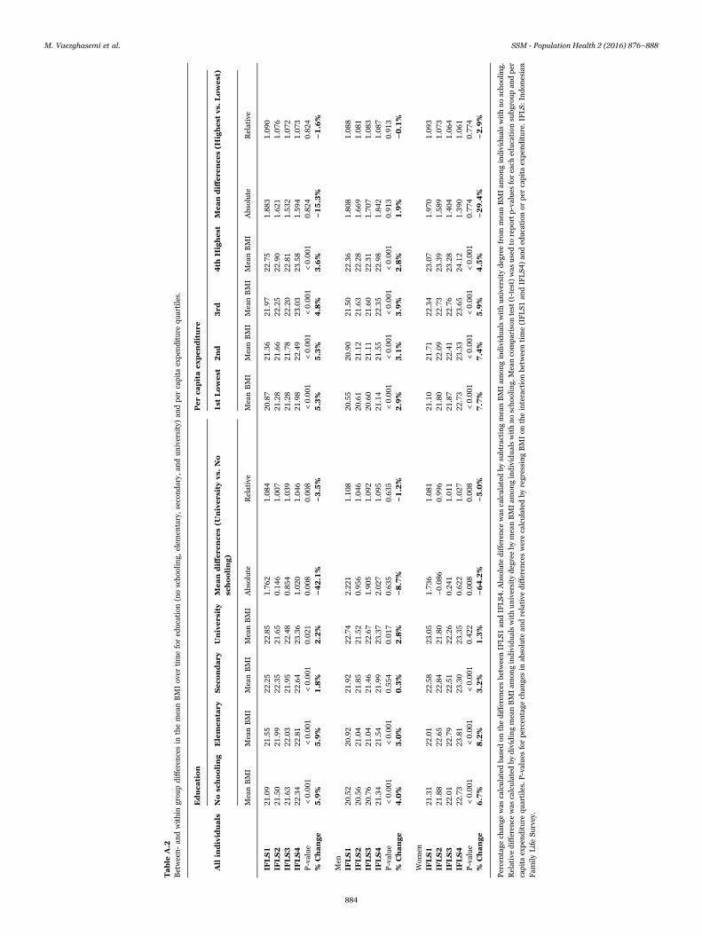
Table

A.2

Between-an

dwithin

grou

pdifferencesin

themeanBMIov

ertimefored

ucation

(noschoo

ling,

elem

entary,secondary,

anduniversity)an

dper

capitaexpen

diture

quartiles.

Educa

tion

Perca

pitaexpenditure

All

individ

uals

Nosc

hooling

Elem

entary

Seco

ndary

Univers

ity

Mean

diff

ere

nce

s(U

nivers

ityvs.

No

schooling)

1st

Lowest

2nd

3rd

4th

Highest

Meandiff

ere

nce

s(H

ighest

vs.

Lowest)

MeanBMI

MeanBMI

MeanBMI

MeanBMI

Absolute

Relative

MeanBMI

MeanBMI

MeanBMI

MeanBMI

Absolute

Relative

IFLS1

21.09

21.55

22.25

22.85

1.76

21.08

420

.87

21.36

21.97

22.75

1.88

31.09

0IF

LS2

21.50

21.99

22.35

21.65

0.14

61.00

721

.28

21.66

22.25

22.90

1.62

11.07

6IF

LS3

21.63

22.03

21.95

22.48

0.85

41.03

921

.28

21.78

22.20

22.81

1.53

21.07

2IF

LS4

22.34

22.81

22.64

23.36

1.02

01.04

621

.98

22.49

23.03

23.58

1.59

41.07

3P-value

<0.00

1<0.00

1<0.00

10.02

10.00

80.00

8<0.00

1<0.00

1<0.00

1<0.00

10.82

40.82

4%

Change

5.9%

5.9%

1.8%

2.2%

−42.1%

−3.5%

5.3%

5.3%

4.8%

3.6%

−15.3%

−1.6%

Men

IFLS1

20.52

20.92

21.92

22.74

2.22

11.10

820

.55

20.90

21.50

22.36

1.80

81.08

8IF

LS2

20.56

21.04

21.85

21.52

0.95

61.04

620

.61

21.12

21.63

22.28

1.66

91.08

1IF

LS3

20.76

21.04

21.46

22.67

1.90

51.09

220

.60

21.11

21.60

22.31

1.70

71.08

3IF

LS4

21.34

21.54

21.99

23.37

2.02

71.09

521

.14

21.55

22.35

22.98

1.84

21.08

7P-value

<0.00

1<0.00

10.55

40.01

70.63

50.63

5<0.00

1<0.00

1<0.00

1<0.00

10.91

30.91

3%

Change

4.0%

3.0%

0.3%

2.8%

−8.7%

−1.2%

2.9%

3.1%

3.9%

2.8%

1.9%

−0.1%

Wom

enIF

LS1

21.31

22.01

22.58

23.05

1.73

61.08

121

.10

21.71

22.34

23.07

1.97

01.09

3IF

LS2

21.88

22.65

22.84

21.80

−0.08

60.99

621

.80

22.09

22.73

23.39

1.58

91.07

3IF

LS3

22.01

22.79

22.51

22.26

0.24

11.01

121

.87

22.41

22.76

23.28

1.40

41.06

4IF

LS4

22.73

23.81

23.30

23.35

0.62

21.02

722

.73

23.33

23.65

24.12

1.39

01.06

1P-value

<0.00

1<0.00

1<0.00

10.42

20.00

80.00

8<0.00

1<0.00

1<0.00

1<0.00

10.77

40.77

4%

Change

6.7%

8.2%

3.2%

1.3%

−64.2%

−5.0%

7.7%

7.4%

5.9%

4.5%

−29.4%

−2.9%

Percentage

chan

gewas

calculatedba

sedon

thedifferencesbe

tweenIFLS1

andIFLS4

.Absolute

difference

was

calculatedby

subtractingmeanBMIam

ongindividualswithuniversity

degreefrom

meanBMIam

ongindividualswithnoschoo

ling.

Relativedifference

was

calculatedby

dividingmeanBMIam

ongindividualswithuniversity

degreeby

meanBMIam

ongindividualswithnoschoo

ling.

Meancomparison

test

(t-test)was

usedto

reportp-values

foreach

education

subg

roupan

dper

capitaexpen

diture

quartiles.P-values

forpercentage

chan

gesin

absolute

andrelative

differenceswerecalculatedby

regressingBMIon

theinteractionbe

tweentime(IFLS1

andIFLS4

)an

ded

ucation

orper

capitaexpen

diture.IFLS:

Indon

esian

Fam

ilyLifeSu

rvey.

M. Vaezghasemi et al. SSM - Population Health 2 (2016) 876–888

884

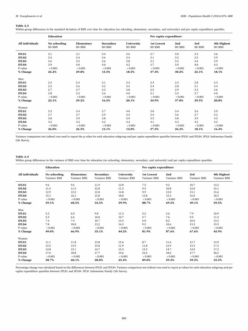
Table A.3Within-group differences in the standard deviation of BMI over time for education (no schooling, elementary, secondary, and university) and per capita expenditure quartiles.

Education Per capita expenditure

All individuals No schooling Elementary Secondary University 1st Lowest 2nd 3rd 4th HighestSD BMI SD BMI SD BMI SD BMI SD BMI SD BMI SD BMI SD BMI

IFLS1 3.1 3.1 3.4 3.6 2.7 3.0 3.3 3.6IFLS2 3.4 3.4 3.6 3.4 3.1 3.3 3.5 3.9IFLS3 3.6 3.5 3.6 3.8 3.1 3.5 3.6 3.9IFLS4 3.9 4.0 4.0 4.2 3.7 3.9 4.0 4.3P-value < 0.001 < 0.001 < 0.001 < 0.001 < 0.001 < 0.001 < 0.001 < 0.001% Change 26.2% 29.8% 15.5% 18.3% 37.4% 30.2% 22.1% 18.1%

MenIFLS1 2.3 2.4 3.1 3.4 2.3 2.4 2.8 3.3IFLS2 2.3 2.6 3.2 3.3 2.4 2.8 3.1 3.4IFLS3 2.7 2.7 3.3 3.8 2.5 2.9 3.3 3.6IFLS4 2.8 3.2 3.6 4.0 3.1 3.2 3.7 4.0P-value < 0.001 < 0.001 < 0.001 < 0.001 < 0.001 < 0.001 < 0.001 < 0.001% Change 22.1% 29.2% 16.2% 20.1% 34.9% 37.0% 29.5% 20.8%

WomenIFLS1 3.3 3.4 3.7 4.0 3.0 3.4 3.6 3.9IFLS2 3.7 3.7 3.9 3.4 3.4 3.6 3.7 4.2IFLS3 3.8 3.9 3.8 3.9 3.5 3.8 3.9 4.2IFLS4 4.2 4.3 4.2 4.4 4.1 4.3 4.2 4.5P-value < 0.001 < 0.001 < 0.001 < 0.001 < 0.001 < 0.001 < 0.001 < 0.001% Change 26.0% 26.5% 13.1% 12.0% 37.5% 26.2% 18.1% 16.4%

Variance comparison test (sdtest) was used to report the p-value for each education subgroup and per capita expenditure quartiles between IFLS1 and IFLS4. IFLS: Indonesian FamilyLife Survey.

Table A.4Within group differences in the variance of BMI over time for education (no schooling, elementary, secondary, and university) and per capita expenditure quartiles.

Education Per capita expenditure

All individuals No schooling Elementary Secondary University 1st Lowest 2nd 3rd 4th HighestVariance BMI Variance BMI Variance BMI Variance BMI Variance BMI Variance BMI Variance BMI Variance BMI

IFLS1 9.6 9.6 11.9 12.8 7.3 9.2 10.7 13.2IFLS2 11.5 11.5 12.8 11.3 9.5 10.8 12.0 15.1IFLS3 12.9 12.5 12.8 14.8 9.9 12.0 13.1 15.6IFLS4 15.2 16.2 15.8 18.0 13.8 15.5 16.0 18.5P-value < 0.001 < 0.001 < 0.001 < 0.001 < 0.001 < 0.001 < 0.001 < 0.001% Change 59.1% 68.5% 33.5% 39.9% 88.7% 69.5% 49.1% 39.5%

MenIFLS1 5.2 6.0 9.8 11.3 5.2 5.6 7.9 10.9IFLS2 5.4 6.6 10.0 10.7 5.7 7.6 9.5 11.3IFLS3 7.4 7.4 10.7 14.3 6.0 8.2 10.6 13.2IFLS4 7.8 10.0 13.2 16.3 9.5 10.6 13.3 15.9P-value < 0.001 < 0.001 < 0.001 < 0.001 < 0.001 < 0.001 < 0.001 < 0.001% Change 49.0% 66.9% 35.1% 44.2% 81.9% 87.6% 67.6% 45.9%

WomenIFLS1 11.1 11.8 13.8 15.6 8.7 11.6 12.7 14.9IFLS2 13.5 13.9 15.0 11.9 11.8 12.9 13.3 17.5IFLS3 14.8 15.1 14.7 15.3 12.5 14.7 14.9 17.2IFLS4 17.6 18.8 17.7 19.6 16.5 18.6 17.7 20.2P-value < 0.001 < 0.001 < 0.001 < 0.001 < 0.001 < 0.001 < 0.001 < 0.001% Change 58.7% 60.1% 28.0% 25.4% 89.0% 59.3% 39.5% 35.5%

Percentage change was calculated based on the differences between IFLS1 and IFLS4. Variance comparison test (sdtest) was used to report p-values for each education subgroup and percapita expenditure quartiles between IFLS1 and IFLS4. IFLS: Indonesian Family Life Survey.

M. Vaezghasemi et al. SSM - Population Health 2 (2016) 876–888

885

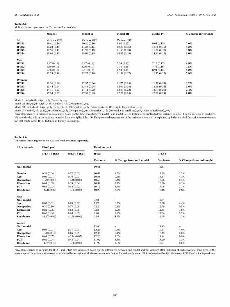
Table A.5Multiple linear regressions on BMI across four models.

Model I Model II Model III Model IV % Change in variance

All Variance (SE) Variance (SE) Variance (SE)IFLS1 10.41 (0.16) 10.40 (0.16) 9.80 (0.15) 9.68 (0.15) 7.0%IFLS2 11.24 (0.15) 11.24 (0.15) 10.80 (0.15) 10.76 (0.15) 4.3%IFLS3 11.96 (0.13) 11.95 (0.13) 11.59 (0.13) 11.56 (0.13) 3.3%IFLS4 15.06 (0.15) 15.06 (0.15) 14.65 (0.15) 14.61 (0.15) 3.0%

MenIFLS1 7.87 (0.19) 7.87 (0.19) 7.24 (0.17) 7.17 (0.17) 8.9%IFLS2 8.39 (0.17) 8.36 (0.17) 7.76 (0.16) 7.76 (0.16) 7.5%IFLS3 9.53 (0.16) 9.51 (0.16) 8.94 (0.15) 8.94 (0.15) 6.2%IFLS4 12.28 (0.18) 12.27 (0.18) 11.58 (0.17) 11.55 (0.17) 5.9%

WomenIFLS1 12.36 (0.26) 12.35 (0.26) 11.75 (0.24) 11.59 (0.24) 6.2%IFLS2 13.44 (0.24) 13.43 (0.24) 13.06 (0.24) 12.96 (0.23) 3.6%IFLS3 14.11 (0.22) 14.11 (0.22) 13.85 (0.22) 13.77 (0.22) 2.4%IFLS4 17.54 (0.25) 17.53 (0.25) 17.27 (0.24) 17.22 (0.24) 1.8%

Model I: bmii=ß0+ß1 (Age)1i+ß2 (Gender)2i+e0iModel II: bmii=ß0+ß1 (Age)1i+ ß2 (Gender)2i+ß3 (Occupation)3i+e0iModel III: bmii=ß0+ß1 (Age)1i+ß2 (Gender)2i+ß3 (Occupation)3i+ß4 (Education)4i+ß5 (Per capita Expenditure)5i+e0iModel IV: bmii=ß0+ß1 (Age)1i+ß2 (Gender)2i+ß3 (Occupation)3i+ß4 (Education)4i+ß5 (Per capita Expenditure)5i+ß6 (Place of residence)6i+e0iPercentage change in variance was calculated based on the differences between model I and model IV. For instance, we subtracted the variance in model I by the variance in model IV.We later divided this by the variance in model I and multiplied it by 100. This gives us the percentage of the variance attenuated or explained by inclusion of all the socioeconomic factorsfor each study wave. IFLS: Indonesian Family Life Survey.

Table A.6Univariate linear regression on BMI and each covariate separately.

All individuals Fixed part Random part

IFLS1 ß (SE) IFLS4 ß (SE) IFLS1 IFLS4

Variance % Change from null model Variance % Change from null model

Null model 10.61 – 16.31 –

Gender 0.35 (0.04) 0.72 (0.03) 10.48 1.2% 15.79 3.2%Age 0.03 (0.01) 0.10 (0.01) 10.55 0.6% 15.61 4.3%Occupation −0.42 (0.08) −0.48 (0.06) 10.57 0.4% 16.26 0.3%Education 0.61 (0.05) 0.13 (0.04) 10.39 2.1% 16.30 0.1%PCE 0.63 (0.03) 0.53 (0.02) 10.12 4.6% 15.96 2.1%Residence −1.28 (0.07) −0.73 (0.06) 10.20 3.7% 16.18 0.8%

MenNull model 7.93 – 12.84 –

Age 0.03 (0.01) 0.09 (0.01) 7.87 0.7% 12.28 4.4%Occupation 0.30 (0.19) 0.77 (0.09) 7.92 0.1% 12.78 0.5%Education 0.82 (0.06) 0.63 (0.05) 7.53 5.0% 12.63 1.6%PCE 0.60 (0.04) 0.63 (0.03) 7.48 5.7% 12.34 3.9%Residence −1.17 (0.09) −0.78 (0.07) 7.59 4.3% 12.69 1.2%

WomenNull model 12.46 – 18.45 –

Age 0.04 (0.01) 0.11 (0.01) 12.36 0.8% 17.54 4.9%Occupation −0.13 (0.10) 0.05 (0.09) 12.45 0.1% 18.45 0.0%Education 0.61 (0.07) −0.14 (0.05) 12.26 1.6% 18.44 0.0%PCE 0.65 (0.04) 0.45 (0.04) 11.92 4.3% 18.20 1.3%Residence −1.37 (0.10) −0.68 (0.09) 11.99 3.8% 18.34 0.6%

Percentage change in variance for IFLS1 and IFLS4 was calculated based on the differences between null model and the variance after inclusion of each covariate. This gives us thepercentage of the variance attenuated or explained by inclusion of all the socioeconomic factors for each study wave. IFLS: Indonesian Family Life Survey; PCE: Per-Capita Expenditure.

M. Vaezghasemi et al. SSM - Population Health 2 (2016) 876–888

886

References

Auld, M. C. (2011). Effect of large-scale social interactions on body weight. Journal ofHealth Economics, 30, 303–316. http://dx.doi.org/10.1016/j.jhealeco.2010.09.002.

Dawson, J. A., Dhurandhar, E. J., Vazquez, A. I., Peng, B., & Allison, D. B. (2013).Propagation of obesity across generations: The roles of differential realized fertilityand assortative mating by body mass index. Human Heredity, 75,204–212. http://dx.doi.org/10.1159/000352007.

Deurenberg, P., Deurenberg-Yap, M., & Guricci, S. (2002). Asians are different fromcaucasians and from each other in their body mass index/body fat percentrelationship. Obesity Reviews, 3, 141–146.

Di Cesare, M., Khang, Y. H., Asaria, P., Blakely, T., Cowan, M. J., Farzadfar, F. et al.(2013). Inequalities in non-communicable diseases and effective responses. Lancet,381, 585–597. http://dx.doi.org/10.1016/S0140-6736(12)61851-0.

Finucane, M. M., Stevens, G. A., Cowan, M. J., Danaei, G., Lin, J. K., Paciorek, C. J. et al.(2011). National, regional, and global trends in body-mass index since 1980:Systematic analysis of health examination surveys and epidemiological studies with960 country-years and 9.1 million participants. Lancet, 377,557–567. http://dx.doi.org/10.1016/S0140-6736(10)62037-5.

Flegal, K. M., & Troiano, R. P. (2000). Changes in the distribution of body mass index ofadults and children in the us population. International Journal of Obesity andRelated Metabolic Disorders, 24,807–818. http://dx.doi.org/10.1038/sj.ijo.0801232.

Gakidou, E. E., Murray, C. J. L., & Frenk, J. (2000). Defining and measuring healthinequality: An approach based on the distribution of health expectancy. The Bulletinof the World Health Organization, 8, 42–54.

Hanandita, W., & Tampubolon, G. (2015). The double burden of malnutrition inindonesia: Social determinants and geographical variations. SSM – PopulationHealth, 1, 16–25. http://dx.doi.org/10.1016/j.ssmph.2015.10.002.

Jones-Smith, J. C., Gordon-Larsen, P., Siddiqi, A., & Popkin, B. M. (2011). Cross-national comparisons of time trends in overweight inequality by socioeconomicstatus among women using repeated cross-sectional surveys from 37 developingcountries, 1989–2007. American Journal of Epidemiology, 173,667–675. http://dx.doi.org/10.1093/aje/kwq428.

Julia, M., van Weissenbruch, M. M., Prawirohartono, E. P., Surjono, A., & Delemarre-vande Waal, H. A. (2008). Tracking for underweight, overweight and obesity fromchildhood to adolescence: A 5-year follow-up study in urban indonesian children.Hormone Research, 69, 301–306. http://dx.doi.org/10.1159/000114862.

Kien, V. D., Van Minh, H., Giang, K. B., Dao, A., Weinehall, L., Eriksson, M. et al. (2016).Socioeconomic inequalities in self-reported chronic non-communicable diseases inurban Hanoi, Vietnam. Global Public Health,1–16. http://dx.doi.org/10.1080/17441692.2015.1123282.

Krishna, A., Razak, F., Lebel, A., Smith, G. D., & Subramanian, S. V. (2015). Trends ingroup inequalities and interindividual inequalities in BMI in the United States, 1993-2012. American Journal of Clinical Nutrition, 101,598–605. http://dx.doi.org/10.3945/ajcn.114.100073.

Merlo, J., Chaix, B., Ohlsson, H., Beckman, A., Johnell, K., Hjerpe, P. et al. (2006). Abrief conceptual tutorial of multilevel analysis in social epidemiology: Usingmeasures of clustering in multilevel logistic regression to investigate contextualphenomena. The Journal of Epidemiology and Community Health, 60,290–297. http://dx.doi.org/10.1136/jech.2004.029454.

Morgan, R., George, A., Ssali, S., Hawkins, K., Molyneux, S., & Theobald, S. (2016). Howto do (or not to do)… Gender analysis in health systems research. Health PolicyPlanning. http://dx.doi.org/10.1093/heapol/czw037.

Murray, C. J. L., Gakidou, E., & Frenk, J. (1999). Health inequalities and social groupdifferences: What should we measure? The Bulletin of the World HealthOrganization, 77, 537–543.

Ogden, C. L., Yanovski, S. Z., Carroll, M. D., & Flegal, K. M. (2007). The epidemiology ofobesity. Gastroenterology, 132,2087–2102. http://dx.doi.org/10.1053/j.gastro.2007.03.052.

de Onis, M., & Lobstein, T. (2010). Defining obesity risk status in the general childhoodpopulation: Which cut-offs should we use? International Journal of PediatricObesity, 5, 458–460. http://dx.doi.org/10.3109/17477161003615583.

Popkin, B. M. (1998). The nutrition transition and its health implications in lower-income countries. Public Health Nutrition, 1,5–21. http://dx.doi.org/10.1079/PHN19980004.

Prospective Studies, Collaboration, Whitlock, G., Lewington, S., Sherliker, P., Clarke, R.,Emberson, J. et al. (2009). Body-mass index and cause-specific mortality in 900 000adults: Collaborative analyses of 57 prospective studies. Lancet, 373,1083–1096. http://dx.doi.org/10.1016/S0140-6736(09)60318-4.

Razak, F., Corsi, D. J., & Subramanian, S. V. (2013). Change in the body mass indexdistribution for women: Analysis of surveys from 37 low- and middle-incomecountries. PLoS Medicine, 10, e1001367. http://dx.doi.org/10.1371/journal.pmed.1001367.

Roemling, C., & Qaim, M. (2012). Obesity trends and determinants in indonesia.Appetite, 58, 1005–1013. http://dx.doi.org/10.1016/j.appet.2012.02.053.

Roemling, C., & Qaim, M. (2013). Dual burden households and intra-householdnutritional inequality in Indonesia. Economics and Human Biology, 11,563–573. http://dx.doi.org/10.1016/j.ehb.2013.07.001.

Rokholm, B., Silventoinen, K., Angquist, L., Skytthe, A., Kyvik, K. O., & Sorensen, T. I.(2011). Increased genetic variance of bmi with a higher prevalence of obesity. PLoSOne, 6, e20816. http://dx.doi.org/10.1371/journal.pone.0020816.

Rokholm, B., Silventoinen, K., Tynelius, P., Gamborg, M., Sorensen, T. I., & Rasmussen,F. (2011). Increasing genetic variance of body mass index during the Swedish obesityepidemic. PLoS One, 6, e27135. http://dx.doi.org/10.1371/journal.pone.0027135.

Silventoinen, K., Rokholm, B., Kaprio, J., & Sorensen, T. I. (2010). The genetic andenvironmental influences on childhood obesity: A systematic review of twin andadoption studies. International Journal of Obesity, 34,29–40. http://dx.doi.org/10.1038/ijo.2009.177.

Silventoinen, K., Kaprio, J., Lahelma, E., Viken, R. J., & Rose, R. J. (2003). Assortativemating by body height and BMI: Finnish twins and their spouses. American Journalof Human Biology, 15, 620–627. http://dx.doi.org/10.1002/ajhb.10183.

Sommer, I., Griebler, U., Mahlknecht, P., Thaler, K., Bouskill, K., Gartlehner, G. et al.(2015). Socioeconomic inequalities in non-communicable diseases and their riskfactors: An overview of systematic reviews. BMC Public Health, 15, 914. http://dx.doi.org/10.1186/s12889-015-2227-y.

Speakman, J. R. (2013). Evolutionary perspectives on the obesity epidemic: Adaptive,maladaptive, and neutral viewpoints. Annual Review of Nutrition, 33,289–317. http://dx.doi.org/10.1146/annurev-nutr-071811-150711.

Strauss, J., Witoelar, V., Sikoki, B., & Wattie, A. M. (March 2009).The fourth wave of theIndonesia Family Life Survey (ifls4): Overview and field report. Wr-675/1-nia/nichd

Uauy, R., & Solomons, N. W. (2006). The role of the international community: Forging acommon agenda in tackling the double burden of malnutrition. SCN News, 32,24–37.

United Nations Economic Commission for Europe (2010). Developing gender statistics:A practical tool. Reference manual prepared by UNECE Task Force on GenderStatistics Traning for Statisticians with contrinution from various experts. Geneva:United Nations.

Table A.7Prevalence of underweight, normal weight, overweight, and obesity among 20–50 year-olds across the four Indonesian Family Life Survey (IFLS) waves.

All individuals

Cross-sectional data Panel data

Underweight Normal weight Overweight Obese Underweight Normal weight Overweight Obese

WHO ASIAN WHO ASIAN WHO ASIAN WHO ASIAN WHO ASIAN WHO ASIAN WHO ASIAN WHO ASIAN

IFLS 1 12.7 12.7 71.4 58.0 13.8 22.8 2.1 6.4 12.8 12.8 73.9 61.8 11.7 20.5 1.5 4.9IFLS 2 12.2 12.2 70.6 56.4 14.3 23.8 3.0 7.6 9.2 9.2 70.9 55.8 16.7 26.5 3.1 8.5IFLS 3 13.1 13.1 68.4 54.0 15.2 24.8 3.2 8.2 8.9 8.9 66.8 49.7 20.1 29.8 4.2 11.6IFLS 4 10.7 10.7 63.7 48.1 20.0 28.5 5.5 12.6 7.1 7.1 56.3 38.9 27.6 34.6 8.9 19.4

MenIFLS 1 12.0 12.0 76.9 69.9 10.2 19.3 1.0 3.8 11.9 11.9 81.1 70.9 6.7 14.9 0.3 2.3IFLS 2 13.1 13.1 75.9 63.1 9.8 19.8 1.1 4.0 10.0 10.0 79.7 65.7 9.7 21.0 0.6 3.3IFLS 3 14.4 14.4 72.9 60.3 11.3 20.5 1.4 4.8 10.0 10.0 75.6 62.3 13.2 22.7 1.2 5.0IFLS 4 12.3 12.3 69.5 55.1 15.1 24.5 3.0 8.0 7.4 7.4 68.9 51.2 20.0 30.7 3.7 10.7

WomenIFLS 1 13.3 13.3 67.2 52.7 16.5 25.6 3.0 8.5 13.4 13.4 69.8 56.7 14.6 23.6 2.2 6.3IFLS 2 11.5 11.5 66.4 51.2 17.7 27.0 4.4 10.4 8.8 8.8 65.9 50.1 20.7 29.6 4.5 11.4IFLS 3 12.0 12.0 64.3 48.1 18.8 28.7 4.9 11.2 8.3 8.3 61.9 42.5 24.0 33.8 5.9 15.4IFLS 4 9.3 9.3 58.6 41.7 24.4 32.2 7.7 16.8 7.0 7.0 49.0 31.8 32.0 36.8 11.9 24.4

M. Vaezghasemi et al. SSM - Population Health 2 (2016) 876–888

887

Usfar, A. A., Lebenthal, E., Atmarita Achadi, E., Soekirman, & Hadi, H. (2010). Obesityas a poverty-related emerging nutrition problems: The case of Indonesia. ObesityReview, 11, 924–928.

Vaezghasemi, M., Öhman, A., Eriksson, M., Hakimi, M., Weinehall, L., Kusnanto, H.et al. (2014). The effect of gender and social capital on the dual burden ofmalnutrition: A multilevel study in Indonesia. PLoS One, 9, e103849. http://dx.doi.org/10.1371/journal.pone.0103849.

Vellakkal, S., Subramanian, S. V., Millett, C., Basu, S., Stuckler, D., & Ebrahim, S. (2013).Socioeconomic inequalities in non-communicable diseases prevalence in India:Disparities between self-reported diagnoses and standardized measures. PLoS One,8, e68219. http://dx.doi.org/10.1371/journal.pone.0068219.

WHO (1995). Physical status: The use and interpretation of anthropometry. Report of aWHO Expert Committee. Who Technical Report Series 854. Geneva: World HealthOrganization.

WHO Expert Consultation. Appropriate body-mass index for Asian populations and its

implications for policy and intervention strategies. Lancet. 2004;363(9403):157-63.PubMed PMID: 14726171. doi: 10.1016/S0140-6736(03)15268-3.

Wilk, M. B., & Gnanadesikan, R. (1968). Probability plotting methods for the analysis ofdata. Biometrika, 55, 1–17. http://dx.doi.org/10.1038/sj.ijo.0801232.

Winkvist, A., Nurdiati, D. S., Stenlund, H., & Hakimi, M. (2000). Predicting under- andovernutrition among women of reproductive age: A population-based study inCentral Java, Indonesia. Public Health Nutrition, 3,193–200. http://dx.doi.org/10.1017/S1368980000000227.

WHO (2000). Obesity: Preventing and managing the global epidemic. Report of a WHOconsultation. World Health Organization Technical Report Series, 894, 1–253.

Zheng, W., McLerran, D. F., Rolland, B., Zhang, X., Inoue, M., Matsuo, K. et al. (2011).Association between body-mass index and risk of death in more than 1 millionAsians. The New England Journal of Medicine, 364,719–729. http://dx.doi.org/10.1056/NEJMoa1010679.

M. Vaezghasemi et al. SSM - Population Health 2 (2016) 876–888

888