Inter-Dealer Trading in Financial Marketsviswanat/journalofbusinesswang.pdf#04409 UCP: BN article # 770413 S. Viswanathan Duke University James J. D. Wang Hong Kong University of Science

#04409 UCP: BN article # 770413

S. ViswanathanDuke University

James J. D. WangHong Kong University of Science and Technology

Inter-Dealer Trading inFinancial Markets*

I. Introduction

Trading between dealers who act as marketmakers is a common feature of most major fi-nancial markets. With the exception of equitymarkets that deal with relatively small ordersizes, in most financial markets the customerorder is filled by one dealer who then retradeswith other dealers. Inter-dealer trading is an in-tegral part of market design, particularly for in-stitutional markets that deal with large orders.While the exact structure of inter-dealer tradingis undergoing significant change (as we discussbelow) two distinct kinds of inter-dealer trading,sequential trading and limit-order books aredominant in the marketplace.In equity markets like the London Stock Ex-

change, inter-dealer trading constitutes some40% of the total volume and occurs mainly viaan anonymous limit-order book, although some

(Journal of Business, 2004, vol. 77, no. 4)B 2004 by The University of Chicago. All rights reserved.0021-9398/2004/7741-0013$10.00

1

* We thank Kerry Back, Dan Bernhardt, Francesca Cornelli,Phil Dybvig, Joel Hasbrouck, Hong Liu, Rich Lyons, AnanthMadhavan, Ernst Maug, Tim McCormick, Venkatesh Pan-chapagesan, Ailsa Roell and seminar participants at Universityof Arizona, Duke University, Hong Kong University of Scienceand Technology, University of Michigan, University of SouthernCalifornia, Virginia Polytechnic University, Washington Uni-versity in St. Louis, the 1999 Nasdaq-Notre Dame Microstruc-ture Conference, and the 1999 WFA Meetings in Santa Monica,California, for their comments. The suggestions of an anony-mous referee considerably improved the paper.

We compare the fol-lowing multi-stageinter-dealer tradingmechanisms: a one-shotuniform-price auction,a sequence of unitauctions (sequentialauctions), and a limit-order book. With unin-formative customerorders, sequentialauctions are revenue-preferred because win-ning dealers in earlierstages restrict quantityin subsequent auctionsso as to raise the price.Since winning dealersmake higher profits,dealers competeaggressively, thusyielding higher cus-tomer revenue. Withinformative customerorders, winning dealersuse their private infor-mation in subsequenttrading, reducingliquidity. Sequentialtrading breaks downwhen the customerorder flow is too infor-mative, while thelimit-order book isrobust and yieldshigher revenues.

#04409 UCP: BN article # 770413

inter-dealer trading occurs through direct negotiation between dealers.The evidence in Hansch, Naik, and Viswanathan (1998), Naik andYadav (1997), and Reiss and Werner (1998) suggests that the layoff oflarge orders (risk sharing) is important reason why inter-dealer tradingoccurs in London. On the NASDAQ market, market makers can tradewith each other on the SuperSoes system, the SelectNet system andon electronic crossing networks (ECNs) like Instinet. The SuperSoessystems allows market makers to place limit orders that are hit byother market makers, electronic crossing networks (ECNs) and daytraders. Volume on SuperSoes is 20% of NASDAQ volume, a sig-nificant portion of this volume is inter-dealer trading. Market makerscan also place quotes on SelectNet system. If these quotes are hit byother market makers (who must place orders that are a hundred sharesmore than the quoted size), the quoting dealer has the discretion toexecute the order or withdraw the quote (this is called discretionaryexecution). Inter-dealer trading on SelectNet is around 10% of totalNASDAQ volume. Finally market makers can trade with each otheron ECNs like Instinet (which includes direct trades between institu-tions); Instinet has around 15% of total NASDAQ volume.1

In the market for U.S. Treasuries, two-thirds of the transactions arehandled by inter-dealer brokerage firms such as Garban and Cantor-Fitzgerald, while the remaining one-third is done via direct inter-actions between the primary dealers. To improve market transparencyin the U.S. Treasuries market, in 1990 the primary dealers and fourinter-dealer brokers founded GovPX, which acts as a disseminator oftransaction price and volume information. Hence, the trading betweenprimary dealers can occur on a number of competing inter-dealerbrokerage systems but is reported via GovPX to financial institutions.2

More recently, the Bond Market Association responded to SEC pres-sure for more transparency in the bond market by setting up a singlereporting system like GovPX for investment grade bonds.3

In the foreign exchange market, inter-dealer trading far exceedspublic trades, accounting for about 85% of the volume.4 Traditionally,inter-dealer trading on the foreign exchange market has been either bydirect negotiation or brokered. Much of the inter-dealer trading viadirect negotiation is sequential (an outside customer trades with dealer1 who trades with dealer 2 who trades with dealer 3 and so on) and

1. See http://www.marketdata.nasdaq.com and http://www.nasdaqtrader.com for thisinformation.

2. The GovPX web sit http://www.govpx.com provides useful information on the historyof GovPX.

3. See the Bond Market Association web site http://www.bondmarkets.com or the relatedwebsite http://www.investinginbonds.com. In an appearance before a House subcommitteeon September 29, 1998, then SEC Chairman Arthur Levitt pushed for greater transparency inbond trading.

4. See Lyons (1995) for more details.

2 Journal of Business

#04409 UCP: BN article # 770413

involves very quick interactions; hence, it is often referred to as ‘‘hotpotato’’ trading. Today, 90% of this direct inter-dealer trading is donevia the Reuters D2000-1 system which allows for bilateral electronicconversations in which one dealer asks another for a quote, which theoriginating dealer accepts or rejects within seconds.5 Brokered tradingis also executed via one of two electronic limit-order book systems,the Reuters Dealing 2002 system and the Electronic Brokerage System(EBS Spot Dealing System). The Reuters Dealing 2002 system waslaunched in 1992 and is discussed extensively by Goodhart, Ito, andPayne (1996). The EBS system was started to compete against theReuters system and claims average volumes in excess of $80 billion aday.6

The preceding discussion makes clear that two distinct kinds ofinter-dealer trading, sequential trading (as in the Reuters D2000-1system) and limit-order books (as in the EBS system, the SuperSoessystem) are most prevalent. In our view, the literature on marketmicrostructure does not explain how the structure of inter-dealer trad-ing should differ according to the underlying trading environment.7

While the seminal work of Ho and Stoll (1983) suggests that risk-sharing is a strong motive behind inter-dealer trading, it is not entirelyclear why risk-sharing needs could not be met optimally by directcustomer trading with several dealers. Even if inter-dealer trading isdesirable, it is unclear which method of inter-dealer trading is moreappropriate. Our view is echoed by Lyons (1996a) in his discussion ofempirical results on the foreign exchange market where he states that‘‘a microstructural understanding of this market requires a much richermultiple-dealer theory than now exists (see e.g. Ho and Stoll 1983).’’In this paper, we provide models of inter-dealer trading that include

both single-price procedures with sequential trading (reflecting the tra-ditional voice-brokering methods of inter-dealer trading) and multiple-price procedures like limit-order books (reflecting the recent movetowards electronic books in the foreign exchange market). Also, we askhow the strategic behavior of dealers and the execution prices for cus-tomer orders differ with the exact structure of the inter-dealer market(single-price auction versus limit-order book) and with the motivationof customer trades (inventory versus information). We believe that

5. This information is provided in Evans and Lyons (2002) that uses the Reuters-2001dataset.6. The EBS partnership is a consortium of banks that are the leading market makers in the

foreign exchange market. One key advantage of the EBS spot dealing system is that it linksautomatically with FXNET, a separate limited partnership of banks that provides for auto-mated netting and hence reduces settlement risk. EBS’s web site http://www.ebsp.com)provides more details. The Reuters web site http://www.reuters.com) provides details on theReuters Dealing 2002 system.7. In the canonical models of Glosten and Milgrom (1985) and Kyle (1985), the outside

order is taken completely by one dealer and no retrading occurs.

3Inter-Dealer Trading in Financial Markets

#04409 UCP: BN article # 770413

realistic modeling of inter-dealer trading is crucial to improve ourunderstanding of dealership markets like the foreign exchange market,the U.S. Treasury market and the NASDAQ market.

Initially, we compare customer welfare between (1) two-stagetrading that involve inter-dealer trading after a customer-dealer tradeand (2) one-shot trading traditionally analyzed in the literature. Weidentify a key advantage of two-stage trading that is absent in one-shottrading environments.

Since Wilson (1979), it is known that single-price divisible goodauctions are plagued with a ‘‘demand reduction’’ problem (see alsoBack and Zender (1993), Wang and Zender (2002), and Ausubel andCramton (2002)). That is, uniform-price auctions have equilibria inwhich prices deviate substantially from economic values becausebidders act strategically and steepen their demand curves. Two-stagetrading alleviates this problem because customers do not split orders inthe first stage, and in the second stage the dealer who wins in the firststage acts strategically. In particular, the dealer who wins in the firststage restricts the supply of the good in the second stage, i.e., engagesin supply reduction. This raises the price in the second stage. Since thewinner in the second stage has a higher utility in the first stage, there isan incentive to bid aggressively for the whole quantity in the firststage. This leads to higher revenue in the two-stage procedure. Theability of two-stage trading to elicit greater bidder competition givesthe seller a potentially powerful weapon to cope with strategic biddingin single-price auction. This idea is worth emphasizing and is useful inunderstanding why multi-stage trading occurs in the real world.

To gain a deeper understanding of the nature of inter-dealer trading,we extend the analysis to the case when the dealers rely on a limit-order book at the second-stage. There are important differences be-tween inter-dealer trading at one price (dealership) and inter-dealertrading at multiple prices (a limit-order book). In contrast to thedealership market, the benefit to a limit-order book market decreaseswith customer order size. In a single-price auction strategic bidding(i.e., a departure from bidding according to marginal valuations) isgreatest at large quantities. In a limit-order book it is the greatest atsmall quantities.8 Therefore, for a limit-order book, the revenue im-provement of a two-stage versus a one-shot trading is mainly for smallcustomer orders.

We generalize our two-stage, single price procedure to a sequentialauction with multiple rounds of unit-auctions. In the sequential auction,the winning dealer (in any round) keeps some fraction of the object and

8. These differences in market makers’ trading strategies across market structures areemphasized in Viswanathan and Wang (2002). The hybrid market structure considered therewas not two-stage trading, but rather a concurrent setup which routes orders to differentmarketplaces using a size criterion.


#04409 UCP: BN article # 770413

sells the remaining via a unit-auction to one of the remaining dealers inthat round. The procedure is in the spirit of the ‘‘voice-brokering’’market where a customer sells to dealer 1 who then sells to dealer 2 andso on. We show that in such a sequential auction market liquidity fallsas the auction progresses, and in each successive round the winningdealer in that round keeps a larger fraction of the order flow for himself.Further, we show that the seller is better off with more rounds ofauctions. These results rationalize the use of sequential auctions andexplain the phenomenon of ‘‘hot potato’’ trading.We extend our analysis to environments where the customer order

flow contains payoff-relevant information. Absent reporting of trades,the information asymmetry between the customer and the marketmakers imposes a cost on inter-dealer trading that adversely affects theattainment of efficient risk-sharing. More asymmetric information inorder flow lowers market liquidity and yields uniformly lower pricecompetition between dealers. With large information asymmetry, a(linear strategy) equilibrium does not exist in a sequential auction. Incontrast, inter-dealer trading with a limit-order book is less sensitiveto private customer information and does not break down. Thus limit-order books are more robust to market breakdown than sequentialauctions.The paper proceeds as follows. Section II discusses the prior liter-

ature and our relation to it. Section III presents a model of two-stagetrading in a dealership setting. The basic intuitions of the model arelaid out in this simple context by comparing customer welfare betweentwo-stage trading and one-shot trading. Section IV analyzes a se-quential auction procedure that extends two-stage trading. The im-portant case of limit-order book trading is taken up in Section V.Section VI deals with informative customer trades; we also comparethe customer’s expected revenues under different trading mechanisms.Section VII concludes.

II. Literature Review

Naik, Neuberger, and Viswanathan (1999) and Lyons (1997) considerthe value of disclosing customer trades and inter-dealer trades indealership markets. The focus of our paper is not on disclosure ofcustomer trades but rather on the comparison of differing inter-dealersystems. Vogler (1997) considers the special case of a dealershipmarket when dealers have the same pretrading inventory and con-cludes that inter-dealer trading always dominates the one-shot deal-ership market. Potential costs to two-stage trading in our model areabsent from Vogler’s model because his is not a model of privateinformation and because he assumes homogeneous inventories acrossthe dealers. None of the above papers considers the limit-order book


#04409 UCP: BN article # 770413

as a possible mode of inter-dealer trading or considers sequentialauction procedures.9 Our modeling of the limit-order book allowsdealers to use limit-orders of arbitrary sizes in the inter-dealing stageand for optimal bidding for the customer trade in the first round.

This paper is also related to the recent literature on limit-order booksdue to Biais, Martimort, and Rochet (2000), Viswanathan and Wang(2002) andRoell (1998). Viswanathan andWang (2002) characterize theequilibria of a dealership market (a single-price setup) and a limit-orderbook (a multi-price setup) when the risk-averse dealers compete for thecustomer order via downward sloping demand curves. Roell (1998)provides related results when the order flow is drawn from the expo-nential distribution. Bias,Martimort, andRochet (2000) characterize thelimit-order book when the marginal valuation curve is downwardsloping due to information in the order flow. Viswanathan and Wang(2002) discusses the relationships between these papers and their rela-tion to the earlier work of Glosten on themonopoly specialist (1989) andon the competitive limit-order book (1994). While these papers char-acterize limit-order books, they do not allow for inter-dealer trading.

Finally, our paper is related to the literature on retrading in auctionsby Haile (2000) and Gupta and Lebrun (1999). In these models,bidders are risk-neutral and re-trading occurs either because the objectwas not allocated to the bidder with the highest valuation (Gupta andLebrun) or because valuations changed and the bidder with the highestvaluation in the second stage is not the highest bidder in the first stage(Haile). In contrast, retrading in our model occurs because dealerswish to share risk and not hold all of the object themselves.

III. Inter-Dealer Trading With a Single-Price Mechanism

A. The Model

There are N > 2 risk-averse dealers (market makers or liquidity pro-viders) in the game. Each dealer can potentially fill a sell order from arisk neutral outside customer10 of size z, which is distributed over theunit interval [0, 1]. The dealers act to maximize a mean-variance de-rived utility of profit with the risk aversion parameter r.11 A typical

9. Werner (1997) presents a double auction model of inter-dealer trading with initiallyidentical dealers. Following the extensive literature on double auctions with unit demands,all dealers in Werner (1997) submit limit orders to buy or sell a fixed amount in the secondstage. Inter-dealer trading is also taken as given in Lyons (1996b), where the focus is on thetransparency of inter-dealer trades.

10. Customer buys are analyzed analogously.11. With single-price inter-dealer trading (modeled as a uniform-price auction), this

quadratic objective function may be derived from the standard assumption of constantabsolute risk-aversion utility functions and normally distributed payoffs. For the limit-orderbook (akin to a discriminatory auction), these assumptions do not imply a quadratic ob-jective function in the dynamic optimization problem.


#04409 UCP: BN article # 770413

dealer, generically referred to as dealer k (k = 1, 2, . . . , N ), is endowedwith an ex ante inventory of Ik , which is drawn from some commonlyknown distribution that has support, [ I ; I ]. We denote the average (perdealer) initial inventory as Q � ð1=NÞSN

k¼1Ik . The underlying assetvalue, u, is normally distributed as N(u; t�1

u ), and u is independent ofthe ex ante inventories, Ik .To isolate the difference between two-stage trading and one-shot

trading, we initially assume that the ex ante dealer inventories are com-mon knowledge among all dealers. The main conclusions are not quali-tatively different when this assumption is relaxed (see Section III.D).Furthermore, we assume that the customer order does not contain infor-mation about the fundamental value of the traded asset. The consequencesof relaxing this assumption will be evaluated in Section VI.As a benchmark, we consider a one-shot trading setup in which the

dealers submit demand schedules to compete for fractions of the cus-tomer order which is split among theN dealers. The focus of this section,however, is two-stage trading in which the outside order is first filled inits entirety by a single dealer before it is divided among all dealers viainter-dealer trading. Order splitting during customer-dealer trading isdisallowed.12 Partly because most dealership markets are not anony-mous, the customer expects to sell to one dealer instead of splitting theorder among several dealers. As such, competition among the marketmakers in the first round is similar to bidding for an indivisible good.We refer to the dealer who wins the customer order as dealer W, and

to any dealer who loses the customer order as dealer L (8L = 1, 2, . . . ,N, L 6¼W ) .13 After the customer-dealer trading, the customer ordersize and transaction price become known to dealer W, but not to theother dealers.14 Consequently, during inter-dealer trading, dealerW cancondition his trading strategy on z, while dealer L cannot. Inter-dealertrading among all N dealers starts shortly after the first round.15 The

12. The ‘‘all-or-nothing’’ assumption is adopted in part to avoid the difficulty of choosingamong the multiple equilibria that result from analyzing a share auction. The main conclusionsof the paper regarding the superiority of two-stage trading over one-shot trading are not drivenby this assumption. What is important is the observation that the winning dealer in the initialcustomer-dealer trading engages in ‘‘supply reduction’’ to raise the inter-dealer price.13. Throughout the paper, the subscript k denotes quantities for a typical dealer k, whereas

the superscript W (or L) denotes quantities for any specific dealer identified as the winning (orlosing) dealer in the first round.14. The issue of trade disclosure is important if the second stage is run as a limit-order

book, since a key aspect of a book is its inability to condition on quantity. In this paper, wedo not pursue issues related to disclosure but focus on the comparison of various modes ofinter-dealer trading. See Naik, Neuberger, and Viswanathan (1999) for a paper that focuseson disclosure and customer welfare in a dealership market.15. In a dynamic setting, dealer W would face the tradeoff between waiting for the next

customer buy to arrive and initiating trading with other dealers right away. By focusing oninter-dealer trading that occurs soon after the customer order is filled by one particulardealer, we are essentially studying markets where the need to lay off the risk associated withan unbalanced portfolio is very significant.


#04409 UCP: BN article # 770413

efficacy of such two-stage trading will be compared to one-shottrading in which the customer can directly trade with many marketmakers.

It is convenient to visualize inter-dealer trading as involving threesteps. First, dealer W hands over his entire holding of the asset,IW þ z, to an auctioneer (the inter-dealer broker). Then, the auc-tioneer solicits bids from all dealers (including dealer W ) in the formof combinations of price and quantity. Further, we restrict the analysisto demand schedules that are continuously differentiable and down-ward slopping. A typical dealer k’s trading strategy, as a function ofthe equilibrium price and possibly his own pretrading net position, isthe quantity that is awarded to him by the auctioneer, xk.

16 Theequilibrium price of the single-price inter-dealer trading, p2, is deter-mined by equating demand and supply. after the auctioneer collectspayment from all winning bids (those with price levels at or above theequilibrium price), the total proceeds are then returned to dealer W andare his to keep. Note that, at the conclusion of the inter-dealer trading,dealer W ’s net holding is xW, while dealer L’s net position is IL þ xL.In other words, xW denotes dealer W ’s final allocation, while xL isdealer L’s trade quantity. Results in the paper need to be interpretedwith this convention in mind.

In the two-stage game, the winning dealer submits a supply curveduring inter-dealer trading. An alternative is for the winning dealer touse the quantity choice as a strategy. However, with two stages oftrading and no adverse selection problem, we can show that thisalternative is revenue inferior for the winning dealers. The case ofwinning dealers making sequential quantity choices is analyzed inSection IV.

A distinct feature of the dealership market is that most transactionstake place at a single price. Therefore, dealer k’s profit at the con-clusion of inter-dealer trading is:

pWk ¼ u xWk þ p2 Ik þ z� xWk

� �; if k previously won the customer order;

pLk ¼ u Ik þ x Lk

� �� p2x

Lk ; if k did not win the customer order:

Differences between inter-dealer trading via a dealership setup (whichinvolves trading at a single-price) and inter-dealer trading via a limit-order book (which involves trading at multiple prices) are discussed inSection V.

16. It is often convenient to express the bidding strategies as the inverse demand schedule,i.e., price as a function of quantity and inventory. To save notation, arguments to the demandschedules are often suppressed.


#04409 UCP: BN article # 770413

For ease of presentation,17 we maintain the following restrictionsthroughout the paper:

IkTu

rt�1u

; 8k;

1

NT

urt�1

u:

With tractability in mind, we restrict our analysis to equilibria of the modelthat are characterized by linear trading strategies. Given the symmetry ofthe problem, we will search for equilibria in which the strategies of thenonwinning dealers (8L 6¼ W ) take the same functional form.

B. Benchmark: A One-Shot Dealer Market

A one-shot model where the customer can trade directly with Ncompeting market makers serves as a benchmark for comparison withthe two-stage trading model just introduced. The following is a nec-essary condition for the equilibrium strategies in a single-price deal-ership market:18

XNj 6¼i

Bxj p; Ij� �Bp

¼ � xi pð Þu� p� rt�1

u Ii þ xi p; Iið Þ½ :

A unique symmetric, linear solution to the above equation is thefollowing:19

xk p; Ikð Þ ¼ gd u� rt�1u Ik � p

� �; 8k ¼ 1; 2; . . . ;N ;

where

gd ¼N � 2

N � 1ð Þrt�1u

: ð1Þ

The equilibrium price and allocations are:

pd ¼ u� rt�1u Q� ðN � 1Þrt�1

u

N � 2

z

N;

xk ¼z

Nþ N � 2

N � 1ðQ� IkÞ: ð2Þ

17. We make these assumptions in order to restrict the discussion to just one side of themarket, i.e., a customer sells and the market makers buy. Relaxing these parameter re-strictions does not affect the conclusions of the paper in any substantive way.18. See Viswanathan and Wang (2002) for a derivation.19. This is similar to Kyle (1989).


#04409 UCP: BN article # 770413

The customer’s total revenue is

Rd ¼ zpd:

At the end of trading, the net inventory positions are as follows:

Ik þ xk ¼ z

Nþ N � 2

N � 1Qþ Ik

N � 1

¼ z

Nþ 2Ik

Nþ N � 2

N

Pj 6¼k Ij

N � 1

� �; ð3Þ

where the term in parenthesis in Eq. (3) is the average inventory of theother N � 1 dealers.

In the ending positions of the dealers (Eq. (3)), the customer order isequally shared. However, each individual dealers’ inventory is over-weighted by ‘‘one extra share’’ and the average inventory of the otherdealers is underweighted correspondingly.20 We will use this obser-vation to provide intuition for the revenue superiority of two-stagetrading.

In submitting bids for the given quantity, each dealer understands theimpact of his trade on the price. Hence a dealer who wishes to buy findsit optimal to steepen his demand curve to reduce the price. This isreferred to as ‘‘demand reduction’’ (see Ausubel and Cramton (2002)for a general discussion of this phenomenon in uniform-price auctions)and results in a price lower than the dealer’s marginal valuation of theobject (see Eq. (2)). Symmetrically, a dealer who wishes to sell hasstrategic incentives to engage in ‘‘supply reduction’’, i.e., to restrict thesupply at every price. This strategic power leads to each dealer over-weighting his own inventory by ‘‘one extra share’’ of inventory.21 Thetwo-stage tradingmodel that we present exploits this strategic incentive.

C. Equilibrium Analysis of the Two-Stage Trading Model

The two-stage trading model is solved using backward induction.Under a dealership structure, the second-stage (i.e., inter-dealer com-petition) can be modeled as a single-price divisible good auction. Thefirst round bidding between the market makers for the customer ordercan be viewed as a unit demand auction with private bidder valuation.With publicly known dealer inventories, the bidders’ valuation iscommon knowledge and the outcome of the first stage bidding isstandard.

20. Without this overweight, the ending inventory would be zNþ Ik

Nþ 1

N

Pj 6¼k Ij. The

overweight of one’s own inventory implies that inventory hedging is incomplete by theend of trading.

21. Note that dealers have equal strategic power with respect to the customer order whichis equally shared.


#04409 UCP: BN article # 770413

1. The Second Round: Inter-Dealer Trading

When the inter-dealer trading results in all trades clearing at a singleprice, the dealers’ equilibrium trading strategies are provided below.Note that the solution in Proposition 1 forms an ex post equilibriumstrategy in that it is independent of the distribution of customer ordersize or the dealer inventories.Proposition 1. If inter-dealer trading occurs at a single price, it has

a unique linear strategy equilibrium characterized by the following tradingstrategies:

xW p; z; IW� �

¼ g2 u� pð Þ þ IW þ z

N � 1; ð4Þ

xL p; IL� �

¼ g2 u� pð Þ � N � 2

N � 1IL; 8L 6¼ W ; ð5Þ

where the price elasticity of demand, g2, is given by:

g2 ¼N � 2

N � 1ð Þrt1u: ð6Þ

Proof. See Appendix I.Using the above equilibrium strategies, it is straightforward to show:

p2 ¼ u� rt�1u Qþ z

N

� �;

xW ¼ N � 2

N � 1Qþ z

Nþ IW þ z

N � 2

� �;

x L ¼ N � 2

N � 1Qþ z

N� IL

� �; 8L 6¼ W : ð7Þ

Thus, the dealers’ net positions at the end of two rounds of trading will be:

xW ¼ 2z

Nþ N � 2

N � 1Qþ IW

N � 1¼ 2 zþ IWð Þ

Nþ N � 2

N

Pj 6¼W Ij

N � 1

!;

ð8Þ

IL þ x L ¼ N � 2

N � 1

z

Nþ N � 2

N � 1Qþ IL

N � 1¼ 2IL

Nþ N � 2

N

zþP

j6¼L Ij

N � 1

!:

ð9Þ

These two expressions are similar to the last two terms of Eq. (3). Becausethis second round of trading involves retrading among the dealers, noadditional ‘‘external’’ supply is available, which explains the absence of a


#04409 UCP: BN article # 770413

term similar to the first term in Eq. (3). The original customer order, z,shows up as part of dealer W ’s pre-inter-dealer-trading inventory. Thus, itreceives ‘‘one share of overweight’’ in W ’s ending inventory position,much like the one-shot trading model where each dealer’s own pre-tradinginventory is overweighted in the final quantity allocation. This is due to the‘‘supply reduction’’ engaged in by dealer W so as to raise the price in thesecond stage. Comparing Eq. (7) with Eq. (2), we have p2 > pd. Hence,dealerW ’s supply reduction raises the price, and consequently dealer L hasan ending inventory that underweights the customer order.

At the conclusion of inter-dealer trading, the customer order is splitunevenly among the dealers, with dealer W retaining an above aver-age fraction, 2/N, and every other dealer retaining a below averagefraction, (N � 2)

[N(N � 1)], of the original customer order z. In

addition, the price is higher during inter-dealer treading than in theone-shot trading model ( p2 > pd). This is an important differencebetween two-stage trading and one-shot trading.

Next we write dealer k’s (8k = 1, 2, . . . , N ) second-stage (certaintyequivalent) utility, depending on whether or not he gets to fill thecustomer order in the first round:

UWk ¼ u xWk � rt�1

u

2

�xWk�2 þ p2

�Ik þ z� xWk

�¼ u

N�2

N�1Qþ z

Nþ Ik þ z

N�2

� � �� rt�1

u

2

N�2

N�1Qþ z

Nþ Ik þ z

N�2

� � �2

þ u� rt�1u Qþ z

N

� � �Ik þ z� N � 2

N � 1Qþ z

Nþ Ik þ z

N � 2

� � �;

ULk ¼ u Ik þ x Lk

� �� rt�1

u

2Ik þ x Lk� �2� p2x

Lk

¼ u Ik þN � 2

N � 1Qþ z

N� Ik

� � �� rt�1

u

2Ik þ

N � 2

N � 1Qþ z

N� Ik

� � �2

� u� rt�1u Qþ z

N

� � �N � 2

N � 1Qþ z

N� Ik

� � �:

From the above, it is straightforward to compute the utility differ-ence between the winning dealer and the losing dealers, which isuseful in analyzing the first stage of customer-dealer trading.

Corollary 1. If inter-dealer trading occurs at a single price, thedifference in dealer k’s second-stage (certainty equivalent) utility be-tween winning and losing the customer order, z, is:

UWk � UL

k ¼ z u� rt�1u

N � 1ð Þ2Ik þ N N � 2ð ÞQþ N � 3

2

� �z

�( );

8k ¼ 1; 2; . . . ;N : ð10Þ


#04409 UCP: BN article # 770413

2. The First Round: Customer-Dealer Trading

For any given customer order z, Corollary 1 suggests that dealer k’sincentives for filling the customer order are based on the followingprivate value function:22

Vk ¼ UWk � UL

k ; ð11Þ

which is strictly decreasing in his own inventory level, Ik. Thus, withoutloss of generality, we can index the dealers in ascending order of theirinventory positions, i.e., I1< I2< . . .< IN .The first stage of trading is an unit auction under complete infor-

mation. The dealer with the lowest ex ante inventory, dealer 1, winsthe customer order, and he pays an amount equal to the reservationprice of the dealer with the second-lowest inventory, dealer 2.Proposition 2. Assume that dealer inventories are publicly known.

If inter-dealer trading occurs at a single price, the customer receivesthe following revenue in the first round of trading:

R1 ¼ z u� rt�1u

N � 1ð Þ2I2 þ N N � 2ð ÞQþ N � 3

2

� �z

�( )� zp1; ð12Þ

where I2 is the second-smallest inventory among all the dealers.Proof . From Eq.s (10) and (11), it is clear that, for any given z,

we have V1 > V2 > . . . > VN .Although the dealers do not know in advance the size of the in-

coming customer order, z, they compete by submitting a series ofquantity-payment pairs, i.e., a demand schedule that states what thetotal payment to the customer, Bk, will be at each potential customerorder size. In particular, the following is a set of equilibrium biddingstrategies (as a function of the customer order size, z):

B1 zð Þ ¼ V2 zð Þ;Bk zð Þ ¼ Vk zð Þ; 8k 6¼ 1:

The tie-breaking rule is that the lower-numbered dealer wins when thesame bid is submitted by more than one dealer.Regardless of the actual customer order sizes, the outcome is always

that dealer 1 wins and pays the customer dealer 2’s reservation priceof V2.

22. Due to the two-stage nature of the model it is not always true that one could directlywork with the certainty equivalent utility in computing the dealers’ optimal trading strategyin the first round. See Lemma 1 in Appendix II for a proof of the validity of the certaintyequivalent approach in our model.


#04409 UCP: BN article # 770413

Customer revenue from two-stage trading versus one-shot tradingcan be evaluated by comparing Eq.s (12) and (2):

p1 � pd ¼rt�1

u

ðN � 1Þ2N 2 � 2

2NðN � 2Þ zþ Q� I2ð Þ �

: ð13Þ

In Eq. (13), there are two effects that could potentially work inopposite directions. The firs is a ‘‘strategic effect’’ that always worksin favor of the two-stage trading game. This is captured by the termproportional to z. The second effect arises due to the surplus extractedby the winning dealer in the first round of a two-round trading model.This ‘‘bidding effect’’ is the term proportional to Q � I2.

The intuition for the strategic effect is as follows. Previously weestablished that in equilibrium all dealers overweight their own in-ventory. This results in the winning dealer retaining an extra share ofthe customer order: dealer W restricts quantity during the inter-dealertrading stage. Restricting the quantity available (‘‘supply reduction’’)to other bidders raises the price in the second round and yields higherprofits to the winning dealer. Since the winner of the customer orderexpects to receive higher profits in inter-dealer trading, all dealerscompete more intensely for the customer order. This yields the stra-tegic term,

rtu�1

N�1ð Þ2�

N 2�22N N�2ð Þ z

�:23

The strategic effect favors two-stage trading. Also, as the customerorder size becomes larger, the winning dealer’s potential profit in thesecond round becomes greater, which implies more intense competi-tion in the first round. Therefore, the net benefit of this strategic effectto two-stage trading (as opposed to one-shot trading) increases as thecustomer order becomes larger.

The bidding effect is related to the surplus extracted by the winningbidder in the first stage. Since the winning bidder has the lowest in-ventory, it must be that Q � I1> 0, i.e., the winning bidder wishes tobuy additional units. This works in favor of the two-stage trading gameas the customer order is allocated to a trader who desires it the most.However, the transaction price is not set by the dealer with the lowestinventory, but rather by the dealer with the second lowest inventory.If Q � I2> 0, the dealer with the second lowest inventory wants tobuy and hence the price favors the two-stage game. If Q� I2> 0, thedealer with the second lowest inventory wants to sell. In this situation,setting the transaction price based on a dealer who does not want to addto his inventory will have a negative impact on the first-stage price.

23. Note that the customer receives p1, not p2. The strategic effect is less thanp2 � pd ¼ rtu�1

NðN�2Þ z because the winning bidder has to be compensated for the risk of hold-ing additional inventory of size z

N, thus lowering the benefit of running the two-stage trading

game for the customer.


#04409 UCP: BN article # 770413

Notice that this bidding effect arises only because of the surplusobtained by the winning bidder. One way to see this is to rewriteEq. (13) as

p1 � pd ¼rt�1

u

N � 1ð Þ2N 2 � 2

2N N � 2ð Þ zþ Q� I1ð Þ �

� rt�1u

N � 1ð Þ2I2 � I1ð Þ;

ð14Þ

where the last term is the only negative term in the equation and reflectsthe surplus extracted by the winning bidder. Note that the size of thebidding effect is affected by the distribution of dealer inventories and notby the customer order size.Corollary 2. Assume that dealer inventories are publicly known.

Relative to the equilibrium price in a one-shot game, pd, the equilib-rium price in the first round of the two-stage game, p1, has twoproperties: (i) p1 as a function of the customer order size z is alwaysflatter (i.e., more price-elastic) than pd; (ii) p1 has a higher intercept(i.e., small-quantity quote) than pd if and only if Q > I2.The bidding effect does not change as customer order sizes change,

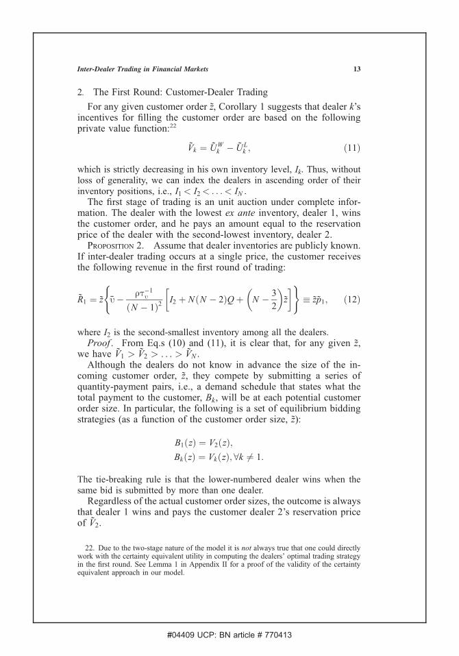
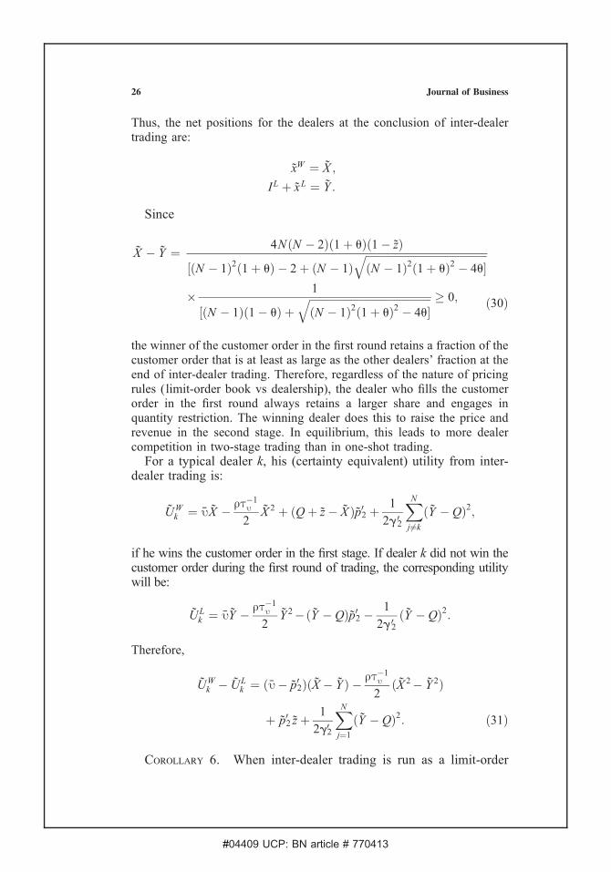
while the strategic effect is proportional to the order size. Thus, thestrategic effect dominates at large order sizes. Therefore, the two-stagedealership market generally provides better execution than its one-shotcounterpart for large-sized order flows. See Figure 1 for an illustration.In empirical work, Naik and Yadav (1997) and Reiss and Werner

(1998) find that the bid-ask spread on inter-dealer trades in smaller thanthe spread on customer-dealer trades. The model here produces thefollowing result, which is consistent with the empirical observation.Corollary 3. If Q � I2 <

ðN�2Þz2N

, then the bid-ask spread on inter-dealer trades is smaller than the spread on customer-dealer trades.From Eq.s (7) and (12), it is easy to see that

p2 � p1 ¼rt�1

u ðN � 2Þ2NðN � 1Þ2

z� rt�1u

ðN � 1Þ2ðQ� I2Þ:

Thus, when the bidding effect (the second-term above) does not dominate(e.g., when the dealer inventories are relatively homogeneous), we havep2 > p1. In this case, the bid price in the second stage is higher than in thefirst stage of trading. An analogous analysis of buy orders reveals that askprices in the second stage are lower than the prices in the first stage oftrading. Thus, the bid-ask spread is smaller on inter-dealer trades.

D. Privately Known Dealer Inventories

Now, any other dealer’s higher private valuation will manifest it-self through a lower value of Q in dealer k’s private value (notice theappearance of Q in Eq. (10)). Thus, when the dealers do not know


#04409 UCP: BN article # 770413

other dealers’ inventory positions, the dealers’ private values are‘‘affiliated’’ in the sense of Milgrom and Weber (1982). Now thecelebrated revenue equivalence theorem does not hold and our choiceof auction form is relevant. For concreteness, we will assume thedealers have exponential preferences and model the customer-dealertrading as a second-price auction.

Proposition 3. Suppose all dealers have exponential preferencesand their inventories are exponentially distributed with a pdf of f (h) =me �mh and a cdf of F(h) = 1�e�mh, where the parameter m> 0.24 Ifthe customer-dealer trading is a second-price auction, then the cus-tomer’s expected revenue is:

R1 � zp1 ¼ z u� rt�1u

ðN � 1Þ2N � 3

2

� �ð2 I þ zÞ

( )

þ ðN � 2Þr

ðm� kÞI2 � lnm

m� k

� � �;

Fig. 1.—Equilibrium price vs customer order size in a dealership market. Thesolid line is for one-shot trading. The three dashed lines are for the initial stageof a two-stage trading model (the second lowest dealer inventory is 0.8,1.0,1.2from top to bottom). The price for two-stage trading is generally higher than itsone-shot counterpart at large customer order sizes, although at small customerorder sizes the comparison is influenced by dealer inventory.

24. For ease of computation, we do not impose the inventory restrictions listed inSection III.A. With the exponential distribution, inventories can be very large. Hence somedealers could be sellers instead of buyers at the single price that clears the second stage.


#04409 UCP: BN article # 770413

where, I2 is the expected value of the second lowest inventory given by:

I2 ¼2N � 1

mNðN � 1Þ ;

and we require k < m:

k � ðN � 2Þr2t�1u

ðN � 1Þ2z:

Proof. See Appendix II.We find that the price the customer expects to receive is usually

higher with two-stage trading than with one-shot trading (for one-shottrading we find pd by integrating Eq. (2) over Q):

p1 � pd ¼N 2rt�1

u

2NðN � 2ÞðN � 1Þ2zþ rt�1

u Q� ð2N � 3ÞðN � 1Þ2

I2

" #

þ ðN � 2Þrz

ðm� kÞI2 � lnm

m� k

� � �: ð15Þ

As in the analysis preceding Eq. (14) in the known inventory case,we can decompose the price difference into two components. The firstis the ‘‘strategic effect’’ which arises because of the supply reductionduring inter-dealer trading. This effect is the first term in Eq. (15)which is strictly positive and proportional to the customer order size.The second line in Eq. (15) is the ‘‘bidding effect’’. As in the known

inventory case, it is typically positive (so long as the log term does notdominate). This effect consists of two effects, the surplus effect andthe winner’s curse (the winner’s curse did not exist with known in-ventories). As before, the surplus effect arises because the price is setby the second lowest inventory in Eq. (15). The winner’s curse arisesbecause the winner does not know the inventories of the bidders belowhim and has to find their conditional expectation. This induces him tounderbid and is reflected in the last term in Eq. (15).Overall, the bidding effect is negative when k approaches m form

below, that is, when the customer order is large and/or when the dealerinventories are drawn from a distribution with high variance. For in-tuition, we recognize that the variance of the exponential distributionis 1/m2. So when m is small, the variance (and mean) of inventories ishigh, suggesting more surplus to the highest type (the dealer with thelowest inventory). Further, the winner’s curse is higher when the var-iance of inventories is higher. Under these circumstances, the biddingeffect works against the two-stage auction.


#04409 UCP: BN article # 770413

The models we have analyzed in Section III all lead to similarconclusions. Two-stage trading enjoys a pricing advantage (from thecustomer’s perspective) over one-shot trading. In two-stage trading,the winning dealer strategically restricts the amount sold in the inter-dealer stage in order to raise the resale price. This strategic effectfavors two-stage trading and is linear in the customer order size. Inaddition, there is a bidding effect that favors two-stage trading unlessthe customer order is large and inventories are drawn from a distri-bution with a high variance.

IV. Sequential Auctions: Rationalizing ‘‘Hot Potato’’ Trading

Much of the inter-dealer trading in the foreign exchange markets is donevia voice-brokering and has the following feature that was emphasizedin the introduction: The customer trades with dealer 1 who trades withdealer 2 who trades with dealer 3, and so on. The quick sequence ofbilateral inter-dealer trades following a customer trade is often re-ferred to as ‘‘hot potato’’ trading. Given our finding in Section III thattwo-stage trading (an unit auction followed by single-price trading) isgenerally favored over one-shot, single-price trading, a logical questionto ask is whether customer welfare is improved by having more tradingrounds.

We construct a sequential trading model of a dealership marketwhere the customer first sells his quantity z to one of N dealers, whothen resells a portion of the customer quantity to another dealer, and soon. This continues until there is a total of m� 4 dealers left, at whichpoint the dealer who has bought in the previous round resells a frac-tion of his quantity to the other m � 1 dealers using a uniform-priceauction. Hence the selling dealer in each round chooses a quantity totrade rather than a supply curve. Thus, the model in this section differsslightly from that in Section III in that a dealer submits a quantityrather than a supply curve. As we will see, the underlying intuition ofrestricting supply to raise the price will still hold.

In this section our focus is on the strategic bidding caused by se-quential trading; thus we assume all dealers are symmetric in their initalinventory positions (set to zero). In other words, the ‘‘bidding effect’’ isabsent here. Also, a dealer who has sold some quantity to another dealercannot trade again. We will refer to the n-dealer stage of sequential trad-ing, which eventually ends when it gets down to m dealers, as an (n, m)trading game, where n � m. When necessary, we use the superscript m

and subscript n to denote quantities in the (n, m) trading game.At the n-dealer stage, the dealer who purchased the quantity qn + 1

from the previous round resells a portion of it, qn , to the other n � 1dealers at the price of pn(qn). We denote the selling dealer’s expectedutility Un and the other dealers’ expected utility Vn.


#04409 UCP: BN article # 770413

We conjecture that the inter-dealer trading price in an (n, m) gametakes the following form:

pnðqnÞ ¼ u� rt�1u lm

n qn: ð16Þ

The parameter lnm is an inverse measure of the market liquidity: the lower

is lnm, the more liquid is the inter-dealer trading.

Proposition 4. In the sequential trading model above, the liquidityparameter is determined by the following iteration formula:

lmnþ1 ¼

lmn

1þ 2lmn

þlmm � 1

2ðm� 1Þðm� 1Þð1þ 2lm

mÞ2ð1þ 2lm

mþ1Þ2. . . ð1þ 2lm

n Þ2;

8n � m � 4; ð17Þ

with lmm = (m � 2)=[(m � 1)(m � 3)].

Proof . See Appendix III.The next result characterizes the evolution of market liquidity, the

dealers’ trading volume and the equilibrium price in the successiverounds of the sequential auction game.Corollary 4. As inter-dealer trading progresses in the (n, m) trading

game (i.e., as n becomes smaller), market liquidity decreases and the sellingdealer retains a larger proportion of the quantity obtained in the previousround. Furthermore, the equilibrium price increases in later rounds.Proof. An inverse measure of market liquidity is ln

m. We firstprove by induction that ln

m is decreasing in n.It is straightforward to verify that lm + 1

m < lmm. Now by assuming

lnm< ln � 1

m , we have:

lmnþ1 ¼

lmn

1þ 2lmn

þlmm � 1


mÞ2ð1þ 2lm

mþ1Þ2. . . ð1þ 2lm

n Þ2

<lmn�1

1þ 2lmn�1

þlmm � 1


mÞ2ð1þ 2lm

mþ1Þ2. . . ð1þ 2lm

n�1Þ2

¼ lmn :

From his optimization problem (see Eq. (A-15) in Appendix III ), theselling dealer retains the following quantity:

qnþ1 � qn ¼2lm

n

1þ 2lmn

qnþ1: ð18Þ


#04409 UCP: BN article # 770413

Thus, the proportion he retains is increasing in lnm. As n becomes smaller,

lnm becomes greater, and therefore, the selling dealer sells less and

chooses to retain a greater share.As for the last statement, multiplying (17) by qn + 1 and using

Eq. (18), it is easy to show that lnmqn is increasing in n. Thus, according

to Eq. (16), price increases as trading progresses (i.e., as n decreases).Corollary 4 demonstrates that the inter-dealer market becomes more

illiquid as trading progresses. This deterioration of liquidity occurs forthe following reasons. Mechanically, as sequential trading evolves,fewer prospective buyers remain. Thus, the potential for risk-sharingwith the remaining participants diminishes. This has a negative impacton the liquidity of the market. Furthermore, the winning dealers insuccessive rounds engage in more quantity restriction by selling lessand withholding a greater share from the inter-dealer market.

The fact that price increases over time is consistent with the two-stage model in Section III (see Corollary 3). As trading unfolds thesellers get higher prices at the expense of worsening liquidity anddeclining trading volume.

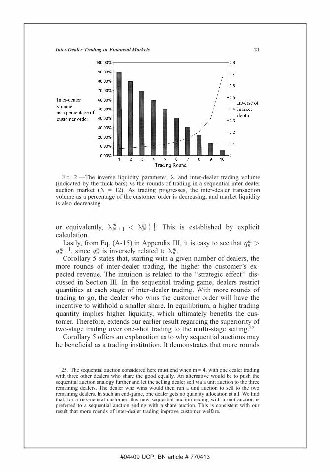
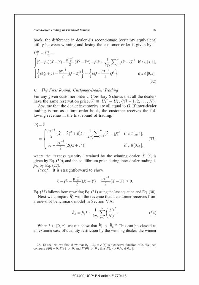
The effects of sequential inter-dealer trading on market liquidity,transactions volume, and dealer competition are illustrated in Figures 2and 3.

Corollary 4 describes the evolution of liquidity, prices and volumealong an auction sequence where the total number of trading rounds isfixed. To draw a closer parallel to the previous comparison of one-shottrading and two-stage trading, we study the customer revenue whenthe number of trading rounds is increased.

Corollary 5. A risk-neutral customer prefers a sequential deal-ership market with more stages of inter-dealer trading. For any givennumber of dealers, when there are more rounds of inter-dealer trading,the trading volume is higher.

Proof . The customer-dealer trade can be viewed as the first roundof trading in the sequential trading game (N + 1, m). Thus, the cus-tomer’s expected revenue is:

E½RmNþ1 ¼ E½zpNþ1ðzÞ ¼

Z 1

0

ðu� rt�1u lm

Nþ1zÞzgðzÞdz: ð19Þ

Now consider a sequential auction with one fewer round of inter-dealer trading, i.e., sequential trading begins as an (N + 1, m + 1)game. In this case, the customer’s expected revenue is:

E½Rmþ1Nþ1 ¼ E½zpNþ1ðzÞ ¼

Z 1

0

ðu� rt�1u lmþ1

Nþ1zÞzgðzÞdz:

To show that the risk-neutral customer always prefers more roundsof inter-dealer trading, it is sufficient to show that E[RN + 1

m ] > E[RN + 1m + 1],


#04409 UCP: BN article # 770413

or equivalently, lN + 1m < lN + 1

m + 1. This is established by explicitcalculation.Lastly, from Eq. (A-15) in Appendix III, it is easy to see that qn

m >qnm + 1, since qn

m is inversely related to lnm.

Corollary 5 states that, starting with a given number of dealers, themore rounds of inter-dealer trading, the higher the customer’s ex-pected revenue. The intuition is related to the ‘‘strategic effect’’ dis-cussed in Section III. In the sequential trading game, dealers restrictquantities at each stage of inter-dealer trading. With more rounds oftrading to go, the dealer who wins the customer order will have theincentive to withhold a smaller share. In equilibrium, a higher tradingquantity implies higher liquidity, which ultimately benefits the cus-tomer. Therefore, extends our earlier result regarding the superiority oftwo-stage trading over one-shot trading to the multi-stage setting.25

Corollary 5 offers an explanation as to why sequential auctions maybe beneficial as a trading institution. It demonstrates that more rounds

Fig. 2.—The inverse liquidity parameter, l, and inter-dealer trading volume(indicated by the thick bars) vs the rounds of trading in a sequential inter-dealerauction market (N = 12). As trading progresses, the inter-dealer transactionvolume as a percentage of the customer order is decreasing, and market liquidityis also decreasing.

25. The sequential auction considered here must end when m = 4, with one dealer tradingwith three other dealers who share the good equally. An alternative would be to push thesequential auction analogy further and let the selling dealer sell via a unit auction to the threeremaining dealers. The dealer who wins would then run a unit auction to sell to the tworemaining dealers. In such an end-game, one dealer gets no quantity allocation at all. We findthat, for a risk-neutral customer, this new sequential auction ending with a unit auction ispreferred to a sequential auction ending with a share auction. This is consistent with ourresult that more rounds of inter-dealer trading improve customer welfare.


#04409 UCP: BN article # 770413

of inter-dealer trading leads to higher expected revenue for the cus-tomer. Consequently, it provides a rationale for the ‘‘hot potato’’phenomenon in the foreign exchange market. Numerical calculationshows that the model can generate trading volumes that rival thesubstantial inter-dealer trading in the foreign exchange market. Forexample, with 12 dealers and 10 rounds of trading, the total inter-dealer trading volume is 4.59 times the initial customer volume: inter-dealer trading is 82% of total volume. This is in line with the numberreported by Lyons (1995) who states that 85% of trading in the foreignexchange market is attributable to inter-dealer trading.

V. Inter-Dealer Trading with a Limit-Order Book

While voice-brokering via sequential trading has traditionally beenused in the foreign exchange markets, much volume has migrated toelectronic limit-order book trading. In particular, as discussed in theintroduction, both the EBS partnership and Reuters Dealing 2002offer systems which have features of a limit-order book. Here weanalyze a two-stage model where the inter-dealer competition occurswithin a limit-order book which is akin to a discriminatory auction.In our analysis of the limit-order book, we assume that all dealer

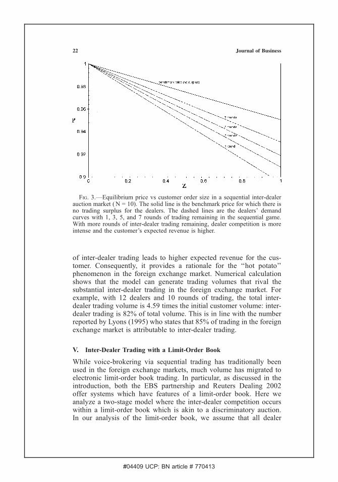
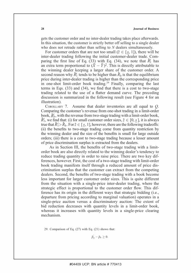
Fig. 3.—Equilibrium price vs customer order size in a sequential inter-dealerauction market ( N = 10). The solid line is the benchmark price for which there isno trading surplus for the dealers. The dashed lines are the dealers’ demandcurves with 1, 3, 5, and 7 rounds of trading remaining in the sequential game.With more rounds of inter-dealer trading remaining, dealer competition is moreintense and the customer’s expected revenue is higher.


#04409 UCP: BN article # 770413

inventories are identical, Ik = Q, k = 1, 2, . . . , N . Then, dealer k’strading profit is:

pWk ¼ u xWk þ p02ðQþ z� xWk Þ þ

XNm6¼k

Z p

p 02

x LmðyÞdy;

pLk ¼ uðQþ x Lk Þ � p02 x

Lk �

Z p

p 02

x Lk ðyÞdy;

where p is the intercept of the demand schedule with the price axis, andp02 is the market clearing price during the inter-dealer trading stage. Weemphasize that, to run the inter-dealer market as an anonymous limit-order book, the customer order in the first stage cannot be disclosed to thedealers who do not receive the order in the first stage.In contrast to the equilibrium in a single-price setting (Section III)

which is independent of distributional assumptions, in this section wesuppose that the distribution of customer order sizes has a linear hazardratio. In particular, the pdf and cdf for z 2 [0, 1] are the following:

gðzÞ ¼ 1

uð1� zÞ1u �1;

GðzÞ ¼ 1� ð1� zÞ1u ;

where u is a positive parameter related to the first two moments of thedistribution as follows:

E½z¼ u

1þ u;

Var½z¼ u2

ð1þ uÞð1þ 3uþ 2u2Þ:

Note that the case of u = 1 corresponds to the uniform distribution.26

A. Benchmark: A One-Shot Limit-Order Book

For comparison purposes, a benchmark is presented in which thecustomer can trade directly with N competing market makers in a one-shot limit-order book. The following is a necessary condition for theequilibrium strategies in a limit-order book market:27

XNj 6¼i

Bxjð pÞBp

¼ � uð1� zÞu� p� rt�1

u ½xið pÞ þ Q :

26. The only other distribution that yields a linear solution is the exponential distribution,which is a limiting case of the linear-hazard ratio class studied here. This can be seen bytaking the limit of GðzÞ ¼ 1� ð1� luzÞ1u as u approaches infinity, which is G(z) = 1� elz.27. See Viswanathan and Wang (2002) for a derivation.


#04409 UCP: BN article # 770413

The unique symmetric, linear solution to the above equation isgiven by:

xkð pÞ ¼ gb u� rt�1u Q� rt�1

u u

Nð1þ uÞ � 1� p

�; 8k ¼ 1; 2; . . . ;N :

where

gb ¼Nð1þ uÞ � 1

ðN � 1Þrt�1u

: ð20Þ

The equilibrium price and allocations are:

pb ¼ u� rt�1u Q� rt�1

u u

Nð1þ uÞ � 1� ðN � 1Þrt�1

u

Nð1þ uÞ � 1

z

N; ð21Þ

xk ¼z

N:

The customer’s total revenue in this case is:

Rb ¼ pb zþXNk¼1

Z p

pb

xkðyÞdy:

Note that dealer positions at the end of trading are as follows:

Ik þ xk ¼z

Nþ Q:

B. The Second Round: Inter-Dealer Trading

With identical ex ante inventories, each dealer has an equal probabilityof winning the customer order in the first stage of trading. Without lossof generality, we designate the dealer who wins the customer order inthe first round of trading as dealer W, and all other dealers are referredto as dealer L. It turns out that dealer W’s equilibrium strategy is inde-pendent of the distributional assumptions about inventory or customerorder size.

Proposition 5. If inter-dealer trading is run as a limit-order book,dealer W ’s equilibrium strategy is:

xW ðp; zÞ ¼u� p

rt�1u

if z 2½s; 1;

Qþ z if z 2½0; s :ð22Þ

8<:


#04409 UCP: BN article # 770413

That is, dealer W will sell a nonzero quantity in the inter-dealer marketif and only if the customer order he fills in the first stage exceeds thefollowing threshold size:

s ¼ 2u

ðN � 1Þð1þ uÞ þ 2uþffiffiffiffiffiffiffiffiffiffiffiffiffiffiffiffiffiffiffiffiffiffiffiffiffiffiffiffiffiffiffiffiffiffiffiffiffiffiffiffiffiffiffiffiffiðN � 1Þ2ð1þ uÞ2 � 4u

q : ð23Þ

Proof. See Appendix IV.The analysis of the optimal strategy for a dealer who did not get to

fill the customer order, dealer L, involves solving a dynamic optimi-zation problem.Proposition 6. Assume that the dealer inventories all equal Q. If inter-

dealer trading is run as a limit-order book, the trading strategy for dealerL is:

xLð pÞ ¼ m02 � g 02 p; 8L 6¼ W ; ð24Þ

where

g 02 ¼

ðN � 1Þð1þ uÞ � 2þffiffiffiffiffiffiffiffiffiffiffiffiffiffiffiffiffiffiffiffiffiffiffiffiffiffiffiffiffiffiffiffiffiffiffiffiffiffiffiffiffiffiffiffiffiðN � 1Þ2ð1þ uÞ2 � 4u

q2ðN � 2Þrt�1

u; ð25Þ

m 02 ¼ g 0

2 u� rt�1u Q� 2rt�1

u u


q264

375:

ð26Þ

Dealer L gets a nonzero quantity allocation if and only if the customerorder size is greater than s.Proof . See Appendix V.For z 2 [s, 1], we can solve for the equilibrium price in the second

stage as:

p 02¼ u� rt�1

u Q� rt�1u

2ðN�1ÞuðN�1Þð1�uÞþ

ffiffiffiffiffiffiffiffiffiffiffiffiffiffiffiffiffiffiffiffiffiffiffiffiffiffiffiðN�1Þ2ð1þuÞ2�4u

p þ z

1þ ðN � 1Þrt�1u g02

: ð27Þ

Therefore, we can express dealer W ’s quantity allocation after the secondstage trading, xW, and dealer L’s acquired quantity from inter-dealertrading, x L, as follows:

xW ¼ u� p02rt�1

u� X ; ð28Þ

xL ¼ m02 � g02 p02 � IL � Y � IL; 8L 6¼ W : ð29Þ


#04409 UCP: BN article # 770413

Thus, the net positions for the dealers at the conclusion of inter-dealertrading are:

xW ¼ X ;

IL þ x L ¼ Y :

Since

X � Y ¼ 4NðN � 2Þð1þ uÞð1� zÞ

½ðN � 1Þ2ð1þ uÞ � 2þ ðN � 1ÞffiffiffiffiffiffiffiffiffiffiffiffiffiffiffiffiffiffiffiffiffiffiffiffiffiffiffiffiffiffiffiffiffiffiffiffiffiffiffiffiffiffiffiffiffiffiðN � 1Þ2ð1þ uÞ2 � 4u

q� 1

½ðN � 1Þð1� uÞ þffiffiffiffiffiffiffiffiffiffiffiffiffiffiffiffiffiffiffiffiffiffiffiffiffiffiffiffiffiffiffiffiffiffiffiffiffiffiffiffiffiffiffiffiffiffiðN � 1Þ2ð1þ uÞ2 � 4u

q � 0; ð30Þ

the winner of the customer order in the first round retains a fraction of thecustomer order that is at least as large as the other dealers’ fraction at theend of inter-dealer trading. Therefore, regardless of the nature of pricingrules (limit-order book vs dealership), the dealer who fills the customerorder in the first round always retains a larger share and engages inquantity restriction. The winning dealer does this to raise the price andrevenue in the second stage. In equilibrium, this leads to more dealercompetition in two-stage trading than in one-shot trading.

For a typical dealer k, his (certainty equivalent) utility from inter-dealer trading is:

UWk ¼ uX � rt�1

u

2X 2 þ ðQþ z� X Þp02 þ

1

2g 02

XNj 6¼k

ðY � QÞ2;

if he wins the customer order in the first stage. If dealer k did not win thecustomer order during the first round of trading, the corresponding utilitywill be:

ULk ¼ uY � rt�1

u

2Y 2�ðY � QÞp02 �

1

2g 02

ðY � QÞ2:

Therefore,

UWk � UL

k ¼ ðu� p02ÞðX � Y Þ � rt�1u

2ðX 2� Y 2Þ

þ p02 zþ1

2g02

XNj¼1

ðY � QÞ2: ð31Þ

Corollary 6. When inter-dealer trading is run as a limit-order


#04409 UCP: BN article # 770413

book, the difference in dealer k’s second-stage (certainty equivalent)utility between winning and losing the customer order is given by:

UWk � UL

k ¼

ðu� p02ÞðX � Y Þ� rt�1

u

2ðX 2� Y 2Þþ p

0

2zþ1

2g02

XN

j¼1ðY �QÞ2 if z 2½s; 1;�

uðQþ zÞ � rt�1u

2ðQþ zÞ2

��uQ� rt�1

u

2Q2

�if z 2½0; s :

8>>><>>>:

ð32Þ

C. The First Round: Customer-Dealer Trading

For any given customer order z, Corollary 6 shows that all the dealershave the same reservation price, V � Uk

W � UkL, (8k = 1, 2, . . . , N ) .

Assume that the dealer inventories are all equal to Q. If inter-dealertrading is run as a limit-order book, the customer receives the fol-lowing revenue in the first round of trading:

R10 ¼V

¼

rt�1u

2ðX � Y Þ2 þ p

0

2zþ1

2g20

XN

j¼1ðY � QÞ2 if z 2½ s; 1;

u z� rt�1u

2ð2Qzþ z2Þ if z 2½0; s :

ð33Þ

8>><>>:

where the ‘‘excess quantity’’ retained by the winning dealer, X –Y , isgiven by Eq. (30), and the equilibrium price during inter-dealer trading isp02, by Eq. (27).Proof. It is straightforward to show:

u� p02 �rt�1

u

2ðX þ Y Þ ¼ rt�1

u

2ðX � Y Þ � 0:

Eq. (33) follows from rewriting Eq. (31) using the last equation and Eq. (30).Next we compare R0

1 with the revenue that a customer receives froma one-shot benchmark model in Section V.A:

Rb ¼ pb zþ1

2gb

XNj¼1

z

N

� �2

: ð34Þ

When z 2 [0, s ], we can show that R10 > Rb.

28 This can be viewed asan extreme case of quantity restriction by the winning dealer: the winner

28. To see this, we first show that R1 � Rb ¼ FðzÞ is a concave function of z . We thencompute F(0) = 0, F( s ) > 0, and F ’(0) > 0 ; thus FðzÞ > 0;8z2½0; s .


#04409 UCP: BN article # 770413

gets the customer order and no inter-dealer trading takes place afterwards.In this situation, the customer is strictly better off selling to a single dealerwho does not retrade rather than selling to N dealers simultaneously.

For customer orders that are not too small (z 2 [s, 1]), there will beinter-dealer trading following the initial customer-dealer trade. Com-paring the first line of Eq. (33) with Eq. (34), we note that R0

1 hasan extra term proportional to (X � Y )2. This is directly attributable tothe winning dealer keeping a larger share of the customer order. Asecond reason why R0

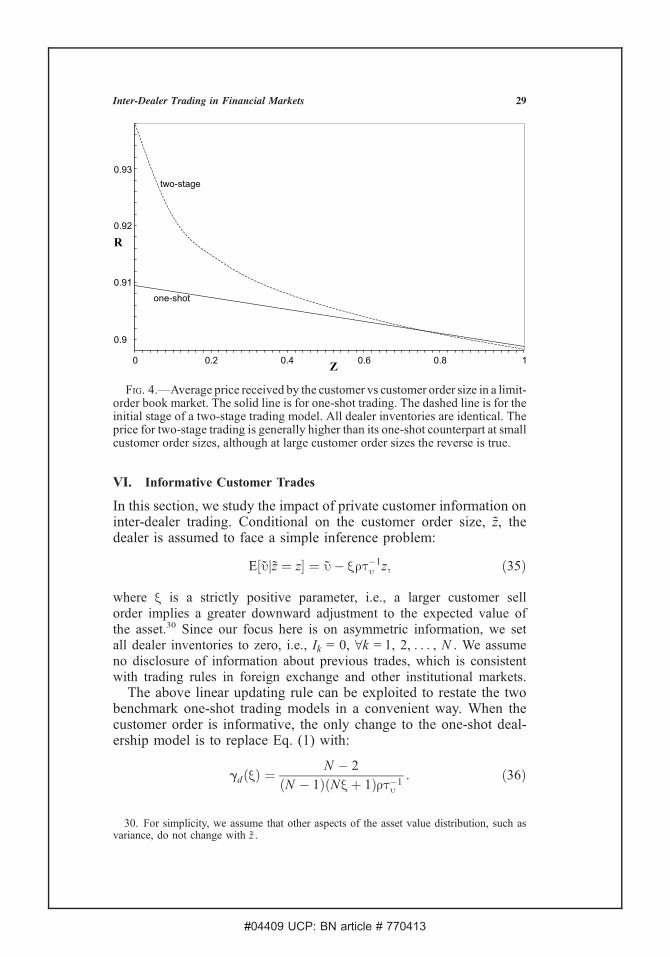
1 tends to be higher than Rb is that the equilibriumprice during inter-dealer trading is higher than the corresponding pricein one-shot limit-order book trading.29 Finally, comparing the lastterms in Eqs. (33) and (34), we find that there is a cost to two-stagetrading related to the use of a flatter demand curve. The precedingdiscussion is summarized in the following result (see Figure 4 for anillustration).

Corollary 7. Assume that dealer inventories are all equal to Q.Comparing the customer’s revenue from one-shot trading in a limit-orderbook, R0

b , with the revenue from two-stage tradingwith a limit-order book,R10 , we find that: (i) for small customer order sizes, z 2 [0, s ], it is always

true that R 01> Rb . For z 2 [ s, 1], however, there are the following tradeoffs:

(ii) the benefits to two-stage trading come from quantity restriction bythe winning dealer and the size of the benefits is small for large outsideorders; (iii) there is a cost to two-stage trading because a lesser amountof price discrimination surplus is extracted from the dealers.

As in Section III, the benefits of two-stage trading with a limit-order book are also directly related to the winning dealer’s tendency toreduce trading quantity in order to raise price. There are two key dif-ferences, however. First, the cost of a two-stage trading with limit-orderbook trading manifests itself through a reduced amount of price dis-crimination surplus that the customer can extract from the competingdealers. Second, the benefits of two-stage trading with a book becomeless important for larger customer order sizes. This is quite differentfrom the situation with a single-price inter-dealer trading, where thestrategic effect is proportional to the customer order flow. This dif-ference has its origin in the different ways that strategic bidding (i.e.,departure from pricing according to marginal valuation) operates in asingle-price auction versus a discriminatory auction: The extent ofbid reduction decreases with quantity levels in a limit-order book,whereas it increases with quantity levels in a single-price clearingmechanism.

29. Comparison of Eq. (27) with Eq. (21) shows that:

p0

2 � pb � 0:


#04409 UCP: BN article # 770413

VI. Informative Customer Trades

In this section, we study the impact of private customer information oninter-dealer trading. Conditional on the customer order size, z, thedealer is assumed to face a simple inference problem:

E½ujz ¼ z ¼ u� xrt�1u z; ð35Þ

where x is a strictly positive parameter, i.e., a larger customer sellorder implies a greater downward adjustment to the expected value ofthe asset.30 Since our focus here is on asymmetric information, we setall dealer inventories to zero, i.e., Ik = 0, 8k = 1, 2, . . . , N . We assumeno disclosure of information about previous trades, which is consistentwith trading rules in foreign exchange and other institutional markets.The above linear updating rule can be exploited to restate the two

benchmark one-shot trading models in a convenient way. When thecustomer order is informative, the only change to the one-shot deal-ership model is to replace Eq. (1) with:

gdðxÞ ¼N � 2

ðN � 1ÞðNxþ 1Þrt�1u

: ð36Þ

Fig. 4.—Average price received by the customer vs customer order size in a limit-order book market. The solid line is for one-shot trading. The dashed line is for theinitial stage of a two-stage trading model. All dealer inventories are identical. Theprice for two-stage trading is generally higher than its one-shot counterpart at smallcustomer order sizes, although at large customer order sizes the reverse is true.

30. For simplicity, we assume that other aspects of the asset value distribution, such asvariance, do not change with z .


#04409 UCP: BN article # 770413

Similarly, in the one-shot limit-order book model (assuming the customerorder is uniformly distributed, i.e., u = 1), we can use:

gbðxÞ ¼2N � 1

ðN � 1ÞðNxþ 1Þrt�1u

; ð37Þ

in place of Eq. (20). These results are quite intuitive because, with aworsening adverse selection problem (a larger x value), the dealers bidless aggressively by steepening their demand curves. From the precedingdiscussion, private customer information tends to make the one-shottrading less competitive.

A. Sequential Auctions

Next we explore the effect of private customer information on thesequential auction model. Since a linear updating rule is assumed forthe customer-dealer trading stage, we conjecture that in subsequentinter-dealer trading the asset value has a similar correlation structurewith the trading quantity. That is:

E½ujqn ¼ u� rt�1u xnqn; ð38Þ

in the (n, m) trading model. Note that, by definition, x N + 1 � x andqN + 1� z.

Suppose inter-dealer trading prices take the form:

pnðqnÞ ¼ u� rt�1u lnqn;

we have the following result.31

Proposition 8. In the sequential trading model with private infor-mation, the liquidity parameter and information parameter are deter-mined by the following iteration formulas:

lnþ1 ¼2lnð1þ 2xnþ1Þ � x2nþ1

2ð1þ 2lnÞþ

lm � xm � 1

2ðm� 1Þm� 1

xn þ 1

xm

� �2

;

8N þ 1 � n � m � 4;

xnþ1 ¼ xn1þ 2ln � xn

;

with lm = (m � 2)[(m � 1)xm + 1][(m � 1)(m � 3)] and xN + 1 = x.

31. In contrast to Section IV, we omit the superscript m in this section to reduce thenotational complexity. It is understood that the number of dealers in the last stage of thesequential game is m.


#04409 UCP: BN article # 770413

Proof . See Appendix VI.Corollary 8. As inter-dealer trading progresses in a sequential

trading game (i.e., as n becomes smaller), both the adverse selectionproblem and market liquidity worsen (i.e., xn + 1< xn and ln + 1< ln).Proof . See Appendix VII.In contrast to the one-shot models where linear strategy equilibria

always exist, with sequential trading the existence of a linear strategyequilibrium is not assured and the presence of informed customertrades may lead to a market breakdown.32

Proposition 9. When the informativeness of the order flow issufficiently high, market breakdown will always occur in sequentialauctions. Fixing the total number of dealers, the parameter region withmarket breakdown expands with the number of trading rounds.Proof . See Appendix VIII.The intuition for a market breakdown is as follows. Because only

the winning dealer observes the customer order flow in the first round,he possesses information about the asset value that other dealers donot have. Recognizing the incentives of the informed dealer to sell agreater share when he perceives a lower asset value, the other dealersrespond by steepening their demand curves. In a multi-auction tradingenvironment, information asymmetry worsens along the auction path.For the same level of quantity traded, the dealers in later trading stagesinfer a lower asset value because this quantity must have resultedfrom a larger quantity sold by the customer (which is taken as a badsignal).As trading progesses, market liquidity worsens and the dealers’

demand curves become more inelastic. At high enough values of theinitial adverse selection parameter x, the inference parameter in the lastround (xm) becomes negative, indicating the nonexistence of a linearstrategy equilibrium. Not surprisingly, the region of breakdown be-comes larger when there are more trading rounds and is the smallestwhen there is one round of inter-dealer trading. The more rounds oftrading, the worse is the market liquidity in the last round. With enoughinitial information asymmetry and enough rounds of trading, we findthat the final round of trading collapses. If the initial informationasymmetry is sufficiently high, more market breakdown occurs (i.e.,market breakdown occurs not just in the last round, but in the final tworounds, final three rounds, etc.) This is discussed in Proposition 9 andillustrated in Figure 5.Comparing the above result with Corollary 5, we see that tension

exists between the strategic advantage implied by running more

32. This ‘‘no-trade’’ result is different from other examples of market breakdown in theliterature (see, e.g., Glosten (1989), Bhattacharya and Spiegel (1991)) in that it occurs withtwo-stage trading but not with one-shot trading.


#04409 UCP: BN article # 770413

auctions and the information disadvantage associated with more inter-dealer trading. In other words, without private information, moretrading rounds benefit the customer because dealers compete for theopportunity to win and gain higher trading profits in subsequent trading.With private information, more trading rounds exacerbate the infor-mation asymmetry problem and have an offsetting effect on customerwelfare. This implies that an interior number of rounds can be optimal(see Figure 5 for illustration).

B. Two-Stage Limit-Order Book Trading

Given the increasing use of limit-order books in the context of inter-dealer trading, it is important to understand how limit-order booktrading is affected by the presence of private information. For thispurpose, we modify the model in Section V by adding a linear in-ference problem (Eq. (35)) to the customer-dealer trading stage.

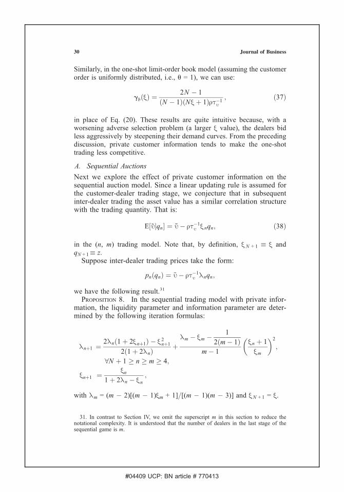
Proposition 10. Assume that customer orders are uniformly dis-tributed over the interval [0,1]. If a limit-order book is used during

Fig. 5.—The maximum feasible and optimal numbers of trading rounds vs theinformation parameter, x , in a sequential auction inter-dealer market ( N = 15). Inthis figure, the higher ‘‘staircase’’ represents the maximum feasible rounds oftrading; the lower ‘‘staircase’’ represents the optimal (from the customer’s per-spective) rounds of trading. When there is little private customer information(when x is small), the number of rounds of inter-dealer trading is relatively highand the two staircases coincide. If the extent of private information is very large(e.g., when x is greater than 2), inter-dealer trading will be made impossible (i.e.,the two staircases fall to zero level, which is not shown in the figure). At inter-mediate values of x , the optimal number of rounds is smaller than the maximumfeasible rounds of trading.


#04409 UCP: BN article # 770413

inter-dealer trading, there exists a linear strategy equilibrium in whichthe strategy for the winning dealer of the customer order is:

xW ð p; zÞ ¼u� xrt�1

u z� p

rt�1u

if z 2½ s; 1;

z if z 2½0; s :ð39Þ

8<:

The inter-dealer trading strategy for dealer L is xL( p) = m � gp, where

g ¼2ðN � 2Þ � Nxþ

ffiffiffiffiffiffiffiffiffiffiffiffiffiffiffiffiffiffiffiffiffiffiffiffiffiffiffiffiffiffiffiffiffiffiffiffiffiffiffiffiffiffiffiffiffiffiffiffiffiffiffiffiffi4NðN � 2Þð1þ xÞ þ N 2x2

q2ðN � 2Þrt�1

u ð1þ NxÞ ;

m ¼

�1þ s

rt�1u

�u� sð1þ xÞ

rt�1u ð1þ xÞ þ ðN � 1Þðrt�1

u x� sÞ ;

s ¼ gu� mrt�1

u ð1þ xÞg ;

s ¼ 1

ðN � 2Þgþ 1

rt�1u

: ð40Þ

Proof . See Appendix IX.It is interesting to compare the way market makers in different inter-

dealer trading systems respond to the problem of private information. Ina dealership setting (e.g., a sequential auction), dealers use increasinglyinelastic demand curves when adverse selection worsens. This phe-nomenon eventually leads to a market breakdown. With a limit-orderbook, however, the winning dealer in the customer-dealer round makestwo adjustments in response to asymmetric information: he lowers theintercept of his demand curve, and he decreases the ‘‘no-trade’’ zone(i.e., increasing s ). It turns out that, for customer orders above a certainthreshold size, a linear strategy equilibrium always exists in limit-orderbook trading.The above result demonstrates that, when inter-dealer trading takes

place in a limit-order book, a linear strategy equilibrium exists evenwhen there is a severe adverse selection problem. This contrasts withsequential auction’s susceptibility to private information. It suggeststhat, in environments where the concentration of informed traders isexpected to be high, inter-dealer trading might well take the form of alimit-order book rather than a sequential auction.


#04409 UCP: BN article # 770413

C. The Customer’s Expected Revenue

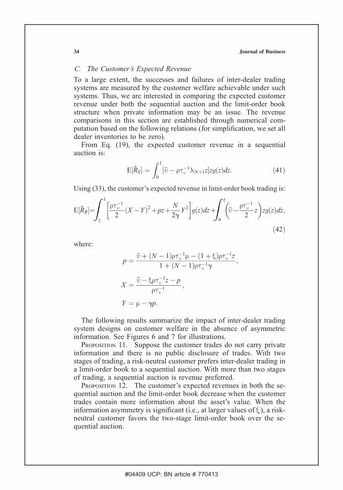
To a large extent, the successes and failures of inter-dealer tradingsystems are measured by the customer welfare achievable under suchsystems. Thus, we are interested in comparing the expected customerrevenue under both the sequential auction and the limit-order bookstructure when private information may be an issue. The revenuecomparisons in this section are established through numerical com-putation based on the following relations (for simplification, we set alldealer inventories to be zero).

From Eq. (19), the expected customer revenue in a sequentialauction is:

E½RS ¼Z 1

0

½u� rt�1u lNþ1zzgðzÞdz: ð41Þ

Using (33), the customer’s expected revenue in limit-order book trading is:

E½RB¼

Z 1

s

rt�1u

2ðX �Y Þ2þpzþ N

2gY 2

�gðzÞdzþ

Z s

0

u� rt�1u

2z

� �zgðzÞdz;

ð42Þ

where:

p ¼ uþ ðN � 1Þrt�1u m� ð1þ xÞrt�1

u z

1þ ðN � 1Þrt�1u g

;

X ¼ u� xrt�1u z� p

rt�1u

;

Y ¼ m� gp:

The following results summarize the impact of inter-dealer tradingsystem designs on customer welfare in the absence of asymmetricinformation. See Figures 6 and 7 for illustrations.

Proposition 11. Suppose the customer trades do not carry privateinformation and there is no public disclosure of trades. With twostages of trading, a risk-neutral customer prefers inter-dealer trading ina limit-order book to a sequential auction. With more than two stagesof trading, a sequential auction is revenue preferred.

Proposition 12. The customer’s expected revenues in both the se-quential auction and the limit-order book decrease when the customertrades contain more information about the asset’s value. When theinformation asymmetry is significant (i.e., at larger values of x), a risk-neutral customer favors the two-stage limit-order book over the se-quential auction.


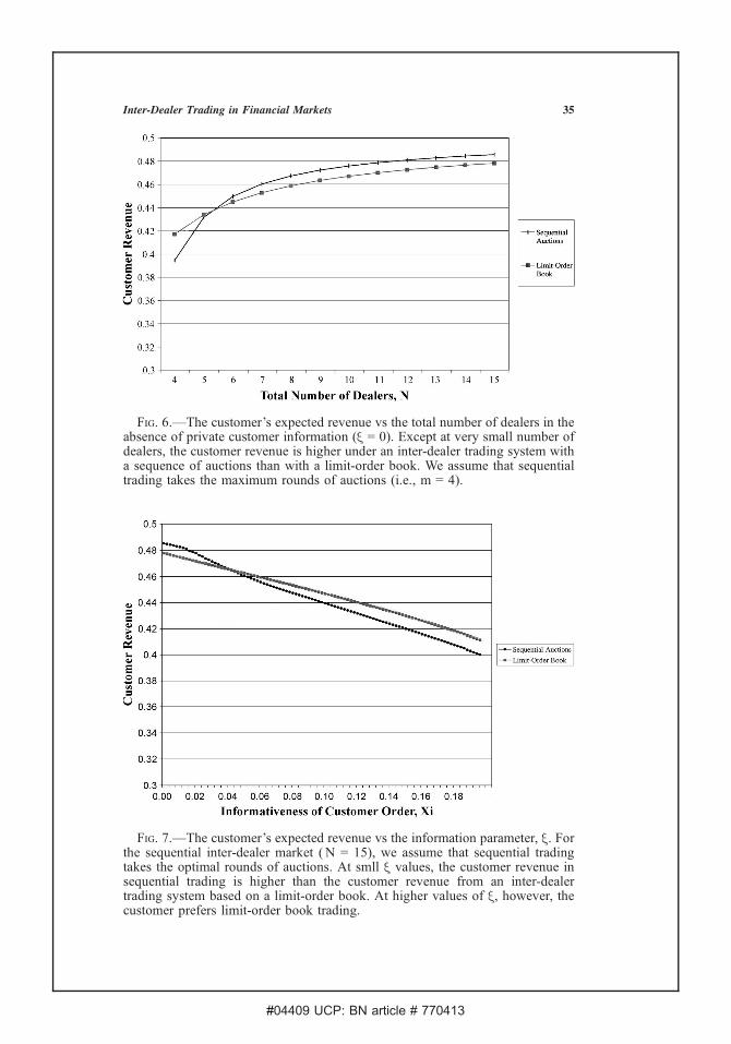
#04409 UCP: BN article # 770413

Fig. 6.—The customer’s expected revenue vs the total number of dealers in theabsence of private customer information (x = 0). Except at very small number ofdealers, the customer revenue is higher under an inter-dealer trading system witha sequence of auctions than with a limit-order book. We assume that sequentialtrading takes the maximum rounds of auctions (i.e., m = 4).

Fig. 7.—The customer’s expected revenue vs the information parameter, x. Forthe sequential inter-dealer market ( N = 15), we assume that sequential tradingtakes the optimal rounds of auctions. At smll x values, the customer revenue insequential trading is higher than the customer revenue from an inter-dealertrading system based on a limit-order book. At higher values of x, however, thecustomer prefers limit-order book trading.


#04409 UCP: BN article # 770413

From Figure 7, it is clear that both E[RS] and E[RB] are decreasingfunctions of x. That is, the presence of asymmetric information has anegative impact on customer welfare in the sequential auction and inthe limit-order book. However, the extent to which private informationadversely affects the customer’s expected revenue differs dependingon the structure of inter-dealer trading.

When private information is nonexistent or unimportant (zero orsmall x values), the auction market (two or more stages) tends to befavored by a risk neutral customer over the two-stage limit-order book.When private information is pervasive (large values of x), the limit-order book is revenue superior to the sequential auction regardless of thenumber of auction rounds inter-dealer trading may take. Proposition 12reinforces the notion that a limit-order book is a better venue for inter-dealer trading when there is a severe adverse selection problem.

VII. Conclusion

In this paper, we study whether multi-stage trading mechanisms thatinvolve inter-dealer trading provide welfare improvement for cus-tomers over the one-shot settings traditionally analyzed in the marketmicrostructure literature. Important determinants of such a comparisoninclude the pricing rules in the inter-dealer market, the size and dis-tribution of the customer orders, the information content of the cus-tomer orders, and, in the case of sequential auctions, the number ofrounds of trading.

We identified a key advantage of multi-stage trading that are absentin one-shot trading environments: the dealer who wins the customerorder restricts the quantity he sells in subsequent rounds so as to raisethe price. As a result, the winning dealer gets an above average fractionof the customer order, thus providing strong incentives for all dealers tocompete more aggressively for the customer order. This intensifiedcompetition leads to improved customer welfare relative to a one-shottrading. Thus, multi-stage procedures are better able to deal with‘‘collusive’’ bidding among market makers that occurs in a one-shotsingle price mechanism. The combination of an ‘‘all or nothing’’ firststage bidding and an active inter-dealer trading phase serves the dualpurpose of facilitating competitive bidding and attaining risk-sharingamong the dealers.

We analyzed a sequential auction model that approximates the tra-ditional voice-brokering in foreign exchange trading. In the sequentialauction, there is repeated bilateral trading between dealers. A back-of-the-envelope calculation shows that the model can generate inter-dealervolumes consistent with the trading volume reported in the literature.Absent private information in the order flow, sequential auctions yieldhigher revenue than limit-order books.


#04409 UCP: BN article # 770413

When informative order flows, in sequential auctions the winningdealer in any given trading round uses his private information insubsequent rounds, reducing the liquidity of the inter-dealer market.Although in equilibrium all information is revealed, the presence ofprivate information distorts risk-sharing and works against the se-quential auction. As a result, the customer’s expected revenue in multi-stage markets decreases with increases in the informativeness of thecustomer order. Of the two kinds of inter-dealer trading, the sequentialauction is more susceptible to market breakdowns than is the limit-order book. A market breakdown always occurs in sequential auctionswhen asymmetric information is high. This argues in favor of using thelimit-order book in inter-dealer trading.Our results provide strong support for inter-dealer mechanisms that

use a sequential auction or a limit-order book. The first corresponds tothe traditional voice-brokering services in the foreign exchange market(and its electronic successor, the Reuters 2000-1 System) while thesecond is closer to the electronic limit-order books like the ReutersDealing 2002 System and the EBS Spot Dealing System.

Appendix A

Proof of Proposition 1

Given the information partition of the dealers, we conjecture the following linearequilibrium strategies:

xW ¼ m0 � g 0pþ b0ðIW þ zÞ;

xL¼ m� gp� b IL; 8L 6¼ W :

Note that dealer W can condition his strategy on z, but dealer L cannot becausethe actual customer order size is only known to dealer W in the first round oftrading.From the market clearing condition

IW þ z ¼ xW þXNL 6¼W

xL;

we can back out dealer W ’s residual supply curve:

p ¼ l xW þ ðN � 1Þm� IW � z� bXNL 6¼W

IL

" #;

where

l ¼ 1

ðN � 1Þg : ðA-1Þ


#04409 UCP: BN article # 770413

Since dealer W already possesses IW + z units of the asset to begin with, he willreceive a payment on the IW + z � xW units that he resells to the other dealersduring inter-dealer trading. For any given set I L, L 6¼ W, dealer W ’s trading profitis therefore:

pW ¼ uxW þ pðIW þ z� xW Þ: ðA-2Þ

Expected utility maximization leads to the following first-order condition fordealer W : 33

0 ¼ u� pþ lðIW þ z� xW Þ � rt�1u xW ; ðA-3Þ

thus,

xW ¼ u� pþ lðIW þ zÞrt�1

u þ l: ðA-4Þ

Comparing Eq. (A-4) with the conjectured functional form, we have:

m0 ¼ urt�1

u þ l; ðA-5Þ

b0 ¼ lrt�1

u þ l; ðA-6Þ

g0 ¼ 1

rt�1u þ l

: ðA-7Þ

Note that the solution obtained does not explicitly depend on I L; thus, it isoptimal for all realizations of I L, L 6¼ W.The analysis of dealer L’s optimal strategy proceeds along similar lines; the only

significant difference is that dealer L cannot condition his strategy on z. In theproof below we fix a specific realization of z and find the trading strategy for dealerL. Since this strategy is independent of z, it is an optimal strategy for all possiblevalues of z.From dealer L’s perspective, the market clearing condition

IW þ z ¼ xL þ xW þXNk 6¼L;W

xk ;

can be used to back out his residual supply curve:

p ¼ s xL þ ðN � 2Þm� IW � z� bXN

k 6¼L;W

Ik þ m0 þ b0ðIW þ zÞ" #

;

33. Since the objective function is concave in xW, the first-order condition is necessaryand sufficient.


#04409 UCP: BN article # 770413

where

s ¼ 1

g0 þ ðN � 2Þg : ðA-8Þ

If he acquires xL units in inter-dealer trading to augment his initial inventory,dealer L will have the following trading profit:

pL ¼ uðIL þ xLÞ � pxL: ðA-9Þ

Expected utility maximization leads to the following first-order condition for L;

0 ¼ u� p� sxL � rt�1u ðIL þ xLÞ;

thus;

xL ¼ u� p� rt�1u IL

rt�1u þ s

: ðA-10Þ

Comparing Eq. (A-10) with the conjectured functional form, we have:

m ¼ urt�1

u þ s; ðA-11Þ

b ¼ rt�1u

rt�1u þ s

; ðA-12Þ

g ¼ 1

rt�1u þ s

: ðA-13Þ

The coefficients (m0, b0, g0 ) and (m , b, g) can be solved from Eq.s (A-1), (A-5),(A-6), (A-7), (A-8), (A-11), (A-12), and (A-13). The solutions are summarized inthe proposition.

Appendix B


First we prove the following lemma which establishes that it is appropriate to usethe difference in certainty equivalent utilities from the second stage (depending onwhether the dealer wins or loses in the first round) as the private value for the unit-demand auction in the first round.Lemma 1. Optimal trading strategies in the first round can be determined by

assuming that each market maker has the private value, V k , which is equal to thedifference in certainty equivalent utility levels when he wins the customer orderand when he does not.


#04409 UCP: BN article # 770413

Proof . Because a dealer uses a demand curve as his trading strategy, the dealercan condition the total payment he makes to the customer (upon winning) onthe size of the customer order. Consequently, in the following we will integrateover the true value of the asset, u, and other dealers’ inventories, I�k , but notover z.Let d be an indicator function which takes on value 1 if dealer k wins the

customer order and value 0 otherwise. Denoting the equilibrium bidding strategyin a second-price auction as Bk and the equilibrium price in the second-round as p2,dealer k’s objective function in the first round is:

Eu; I�k½�e�rfd½u xW

kþ p2ðIkþz�xW

kÞ�Bk þð1�dÞ½uðIkþx L

kÞ�p2 x

Lkg

¼ Eu; I�k½�e�ru½d xW

kþð1�dÞðIkþx L

kÞ�rd½ p2ðIkþz�xW

kÞ�Bk �rð1�dÞp2 x L

k

¼ EI�k½�e

�rfu½d xWkþð1�dÞðIkþx L

kÞ� rt�1

u2

½dxWkþð1�dÞðIkþx L

kÞ2g

�rd½ p2ðIk þ z� xWk Þ � Bk � rð1� dÞp2 x Lk�

¼ EI�k½�e�rdðUW

k� Bk Þ�rð1�dÞUL

k

¼ EI�k½�e�rUL

k EI�k½e�rdðUW

k�UL

k�Bk Þ:

Notice that U kL is independent of I�k and thus we are left with an objective

function which is proportional to the objective function of a bidder in a standardsingle-unit auction with private value of UW

k � ULk .

The above proof assumes that the inter-dealer trading occurs at a single price. Itcan be easily adapted to show that the certainty equivalent approach is also validwhen the customer order is informative about the value of the asset according toEq. (35).Suppose dealer l holds the smallest inventory among all dealers other than k. Let

m be any dealer who is neither k nor l. A result from Milgrom and Weber (1982)( page 1114) states that the equilibrium bidding strategy in a second-price auctionas a function of private values, Bk (x), is the unique solution to:

E �e�r½Vk�Bk ðxÞjIk ¼ x; Il ¼ x; Im � x; 8m 6¼ k; lh i

¼ �e�r�0; ðA-14Þ

where V k is bidder k’s private value of the asset, given by Eq. (11):

Vk ¼ z u� rt�1u

ðN � 1Þ2Ik þ NðN � 2ÞQþ N � 3

2

� �z

�( ):


#04409 UCP: BN article # 770413

For any given z, Eq. (A-14) can be inverted to give:

BkðxÞ ¼ � 1

rlnE½e�rVk jIk ¼ x; Il ¼ x; Im � x

¼ � 1

rlnE

"e�rz

nu � rt�1

uðN�1Þ2

hIkþðN�2Þ

$Ik þ Il þ

PN

m 6¼k; lIm

%þðN � 3

2Þzio

jIk ¼ x; Il ¼ x; Im � x

#

¼ z u� rt�1u

ðN � 1Þ2xþ 2ðN � 2Þxþ N � 3

2

� �z

�( )

� N � 2

rln

Z I

x

e

ðN�2Þr2t�1u

ðN�1Þ2 zyf ðyÞdy

" #:

Therefore, dealer k’s bidding strategy (i.e., total payment for a customer order ofsize z ) expressed as a function of his inventory is:

BkðIkÞ ¼ z u� rt�1u

ðN � 1Þ2N � 3

2

� �ð2 Ik þ zÞ

" #

� N � 2

rln

Z I

Ik

e

ðN�2Þr2t�1u


" #:

The seller’s expected revenue takes the expectation of the above expression overI k = I2 (the second-lowest inventory):


ðN � 1Þ2N � 3

2

� �ð2 I2 þ zÞ

" #� NðN � 1ÞðN � 2Þ

r

�

Z I

I

ln

Z I

he

ðN�2Þr2t�1u


" #f ðhÞFðhÞ½1� FðhÞN�2

dh:

where I2 denotes the expected second-lowest inventory level N(N � 1)R IIh f ðhÞFðhÞ½1� FðhÞN�2

dh.The above explicit solution involves the distribution characteristics of the dealer

inventories. In general, the payment function Bk is not quadratic in the customer


#04409 UCP: BN article # 770413

order size z, i.e., the unit (bid) price is nonlinear in z.34 Take the example of expo-nentially distributed dealer inventories with the parameter m > 0. That is, f (h ) =me�mh and F(h) = 1 � e�mh.For a given z, the customer’s expected revenue is:


ðN � 1Þ2N � 3

2

� �2ð2N � 1ÞmNðN � 1Þ þ z

�( )

þ ðN � 2Þr

m� km

� �2N � 1

NðN � 1Þ � lnm

m� k

� � �;

where we require k<m.

Appendix C


Analyzing the selling dealer’s maximization problem:

maxqn

Un ¼ uðqnþ1 � qnÞ �rt�1

u

2ðqnþ1 � qnÞ2 þ qn pnðqnÞ;

provides the following optimal quantities.35

qn ¼1

1þ 2lmn

qnþ1; ðA-15Þ

Un ¼ qnþ1 u� lmn

1þ 2lmn

rt�1u qnþ1

� �: ðA-16Þ

Notice that the above expected utility for the selling dealer is net of the price thathe paid for the quantity qn + 1 obtained in the previous round of trading. For eachdealer to be just indifferent between receiving or not receiving qn + 1, it must be that:

Un � qnþ1 pnþ1ðqnþ1Þ ¼ Vn:

For dealers other than the seller, their expected utility is a constant at any stageof the game, i.e., Vn = Constant, 8n. To determine this constant, we examine thelast inter-dealer trading stage (i.e., when n = m). Using Eq. (2), the selling price is:

pmðqmÞ ¼ u� ðm� 2Þrt�1u

ðm� 3Þqm

m� 1� u� rt�1

u lmmqm:

34. With known dealer inventories, the unit price is linear in z. See Eq. (12).35. Since ln

m > 0, the second-order condition is always satisfied.


#04409 UCP: BN article # 770413

From the above formula, lmm ¼ m� 2

ðm� 1Þðm� 3Þ. The expected utility for a dealerwho buys in the last round is:

Vm ¼ uqm

m� 1� rt�1

u

2

qm

m� 1

$ %2� pmðqmÞ

qm

m� 1

¼lmm � 1

2ðm� 1Þm� 1

rt�1u q2

m:

Thus, using Eq. (A-15) recursively, we have:

Vn ¼ Vm ¼lmm � 1

2ðm�1Þm� 1

rt�1u q2

m ¼lmm � 1

2ðm�1Þm� 1

rt�1u

qmþ 1

ð1þ 2lmmÞ

�2

¼ . . . ¼lmm � 1

2ðm�1Þm� 1

rt�1u

qnþ 1

ð1þ 2lmmÞð1þ 2lm

mþ1Þ . . . ð1þ 2lmn Þ

�2:

Finally, the price at the (n + 1, m) trading game can be determined as follows:

pnþ1ðqnþ1Þ ¼1

qnþ1

ðUn � VnÞ

¼ u� rt�1u lm

n

1þ 2lmn

qnþ1 �lmm � 1

2ðmþ1Þm� 1

� rt�1u qnþ1

ð1þ 2lmmÞ

2ð1þ 2lmmþ1Þ

2. . . ð1þ 2lm

n Þ2

� u� rt�1u lm

nþ1qnþ1:

Thus, we have the following iteration formula for the liquidity parameter in an(n + 1, m) game:

lmnþ1 ¼

lmn

1þ 2lmn

þlmm � 1

2ðm�1Þ

ðm� 1Þð1þ 2lmmÞ

2ð1þ 2lmmþ1Þ

2. . . ð1þ 2lm

n Þ2:

Appendix D


Suppose the dealer Ls plays the strategy, xL( p), which does not depend on therealization of z (only dealer W observes the true customer order size going into theinter-dealer trading stage).


#04409 UCP: BN article # 770413

If dealer W intends to retain xW< Q + z units after the second round of trading,then his inter-dealer trading profit is:

pW ¼ uxW þ pðQþ z� xW Þ þXNj 6¼W

Z p

p

xjðyÞdy; ðA-17Þ

where p is the intercept of dealer j’s demand schedule with the price axis.Maximization of dealer W ’s expected utility is equivalent to maximizing the

following objective function:

uxW þ pðQþ z� xW Þ� rt�1u

2ðxW Þ2 þ

XNj 6¼W

Z p

p

xjðyÞdy;

which leads to the first-order condition for dealer W:

0 ¼ u� pþ Bp

BxWðQþ z� xW Þ � rt�1

u xW� Bp

BxW

XNj6¼W

xjð pÞ

¼ u� p� rt�1u xW :

The market clearing condition Q + z = xW +PN

j 6¼W xj ( p) is used in the last step.Thus far, we have proved that the trading strategy:

xW ð pÞ ¼ u� p

rt�1u

;

is the equilibrium strategy for dealer W.In the proof of Proposition 6, we will show that there exists a unique cutoff

customer order size, s , such that dealer W is a net seller during inter-dealer tradingif and only if z 2 [s, 1]. Should dealer W decide to use the strategy xW( p) when heobserves a z value that is less than s (based on the incorrect assumption that allother dealers get a positive amount), it can be shown that dealer Ls’ quantityallocation would be negative in that case. This cannot happen in equilibrium,therefore, dealer W retains all of the customer order he fills if it is sufficiently small(i.e., when z < s ).

Appendix E


This proof consists of three parts. By conjecturing that dealerWwill trade in the inter-dealer market only if the customer order is greater than a threshold size 0 < s < 1,we first establish an ordinary differential equation (ODE) as the necessary conditionfor dealer L’s equilibrium trading strategies. Then we explicitly solve for a linearsolution to the ODE. In the last step, we verify the existence of such a thresholdcustomer order size, s .


#04409 UCP: BN article # 770413

In the following we characterize dealer i’s optimal trading strategy, xi ( p) (wesometimes write dealer i’s upward-sloping residual supply curve as h( p)) in re-sponse to the strategy used by the other dealers, xj ( p) (8j 6¼ i ). We use g(z) andG(z)to denote the pdf and cdf for the customer order size z when it falls within [ s, 1].We can write dealer i’s uncertain trading profit as follows:

pi ¼ uxið pÞ � TPi; i 6¼ W ;

where his total payment is:

TPi ¼ ð1� aÞpxið pÞ þZ xið pÞ

0

pðqÞdq

¼ ð1� aÞpxið pÞ þ"XN

j¼1

Z xjð pÞ

0

pðqÞdq�XNj6¼1

Z xjð pÞ

0

pðqÞdq#

� ð1� aÞpxið pÞ þ ½A� B:

We note the following relations for use in subsequent calculation:

BA

Bz¼XNj¼1

pBxj

Bz¼ p

BðQþ zÞBz

¼ p;

and

BB

Bp¼XNj6¼i

pBxjð pÞBp

¼ �pBhð pÞBp

; ðA-18Þ

where we make use of the market clearing condition:

Qþ z ¼ xw þXNi 6¼W

xi:

We assume that dealer i chooses his optimal trading strategy by maximizing thefollowing derived mean-variance utility function:

Ez

uhð pÞ � rt�1

u

2h2ð pÞ � TPi

�:

Defining A(z) as the state variable and p(z) the control variable, we can analyzethe problem using the following Lagrangian:

L ¼ gðzÞuhð pÞ � rt�1

u

2h2ð pÞ � AðzÞ þ Bð pÞ

�þ lp:


#04409 UCP: BN article # 770413

The optimality condition is:

0 ¼ BL

Bp¼ gðzÞ½u� p� rt�1

u hð pÞ Bhð pÞBp

þ l: ðA-19Þ

The adjoint equation is:

� BlBz

¼ BL

BA¼ �gðzÞ; ðA-20Þ

with the transversality condition

lðsÞ ¼ �1:

Using the transversality condition, the adjoint equation can be integrated toobtain

lðzÞ ¼ �½1� GðzÞ: ðA-21Þ

Combining Eqs. (A-19) and (A-21), we have:

½u� p� rt�1u hð pÞ Bhð pÞ

Bp¼ 1� GðzÞ

gðzÞ ; ðA-22Þ

which is equivalent to:

XNj 6¼i

x 0jð pÞ ¼ � ½1� GðzÞ=gðzÞu� p� rt�1

u xið pÞ: ðA-23Þ

Motivated by dealer W ’s use of a linear bidding strategy, we now search for alinear strategy equilibrium of the form:

xk ¼ m� gp; ðA-24Þ

for dealers k. With this, the market clearing condition is:

Qþ z ¼ xW þ xk þ ðN � 2Þðm� gpÞ:

The hazard ratio for z over the interval [ s , 1] is:

1� GðzÞgðzÞ ¼ uð1� zÞ ¼ u½Qþ 1� xW � xk � ðN � 2Þðm� gpÞ: ðA-25Þ


#04409 UCP: BN article # 770413

Plugging Eqs. (22), (A-24), and (A-25) into Eq. (A-23), we obtain:

1

rt�1u

þ ðN � 2Þg ¼u Qþ 1� u� p

rt�1u

� ðN � 1Þðm� gpÞ �

u� p� rt�1u ðQþ xkÞ

;

which can also be written as:

xk ¼1

rt�1u

ð1þ usrt�1u

ðu� pÞþusðN � 1Þðm� gpÞ� usðQþ 1Þ � rt�1u Q

�;

with

s ¼ 1

1

rt�1u

þ ðN � 2Þg:

Because of the symmetry among the N � 1 dealers other than dealer W, we musthave:

g ¼ 1

rt�1u

�1þ us

rt�1u

�þ usðN � 1Þg

�;

m ¼ 1

rt�1u

�1þ us

rt�1u

�uþ usðN � 1Þm� usðQþ 1Þ � rt�1

u Q

�:

The solutions to the above equations are:

g ¼ðN � 1Þð1þ uÞ � 2þ

ffiffiffiffiffiffiffiffiffiffiffiffiffiffiffiffiffiffiffiffiffiffiffiffiffiffiffiffiffiffiffiffiffiffiffiffiffiffiffiffiffiffiffiffiffiðN � 1Þ2ð1þ uÞ2 � 4u

q2ðN � 2Þrt�1

u;

m ¼ g u� rt�1u Q� 2rt�1

u u

ðN þ 1Þð1þ uÞ þ 2uþffiffiffiffiffiffiffiffiffiffiffiffiffiffiffiffiffiffiffiffiffiffiffiffiffiffiffiffiffiffiffiffiffiffiffiffiffiffiffiffiffiffiffiffiffiðN � 1Þ2ð1þ uÞ2 � 4u

q264

375:

Given the above solutions, it can be checked that the following choice ofthreshold customer order size:

s ¼ 2u


q 2ð0; 1Þ;

is a unique number that satisfies the requirements that Q + z � xW and xk � 0,8k 6¼ W for z 2 [ s , 1].This last statement completes the proofs of Propositions 5 and 6.


#04409 UCP: BN article # 770413

Appendix F


We can analyze the selling dealer’s maximization problem:

maxqn

Un ¼ ðu� rt�1u xnþ1qnþ1Þðqnþ1� qnÞ �rt�1

u

2ðqnþ1 � qnÞ2 þ qn pnðqnÞ;

which provides the following optimal quantities:36

qn ¼1þ xnþ1

1þ 2ln

qnþ1 � dnqnþ1;

Un ¼ qnþ1 u�2lnð1þ 2xnþ1Þ � x2nþ1

2ð1þ 2lnÞrt�1

u qnþ1

�: ðA-26Þ

Using Eq. (36), the equilibrium strategy in the last stage of the game (where onedealer sells to m � 1 other dealers) is:

xkðxÞ ¼ gdðxÞðu� pÞ;

where

gdðxÞ ¼m� 3

ðm� 2Þ½ðm� 1Þxm þ 1rt�1u

:

Thus, the equilibrium price there is:

pm ¼ u� rt�1u lmqm;

with

lm ¼ ðm� 2Þ½ðm� 1Þxm þ 1ðm� 1Þðm� 3Þ ðA-27Þ

In addition, the expected utility for those bidding dealers is:

Vm ¼lm � xm � 1

2ðm�1Þm� 1

rt�1u q2m:

Using Eq. (A-26), the above can be rewritten as:

Vn ¼ Vm ¼lm � xm � 1

2ðm�1Þðm� 1Þ rt�1

u ðqmþ1dmÞ2

¼ . . . ¼lm � xm � 1

2ðm�1Þðm� 1Þ rt�1

u ðqnþ1dmdmþ1 . . . dnÞ2:

36. The second-order condition, 1 + 2ln > 0, is satisfied since ln > 0 in equilibrium.


#04409 UCP: BN article # 770413

Note that the expected utility for the nonwinning dealers in each stage must be thesame.Thus, the price at the (n + 1)-th stage can be determined as follows:

pnþ1ðqnþ1Þ ¼ 1

qnþ1

ðUn � VnÞ

¼ u�2lnð1þ 2xnþ1Þ � x2nþ1

2ð1þ 2lnÞrt�1

u qnþ1

�lm � xm � 1

2ðm�1Þm� 1

ðdmdmþ1 . . . dnÞ2rt�1u qnþ1:

Thus, we derive the following iteration formula for the liquidity parameter:

lnþ1 ¼2lnð1þ 2xnþ1Þ � x2

nþ1

2ð1þ 2lnÞþ

lm � xm � 12ðm�1Þ

m� 1ðdmdmþ1 . . . dnÞ2: ðA-28Þ

Because the optimal quantity qn is linear in qn +1 (the quantity traded in theprevious round; see Eq. (A-26)), qn must be linear in z, the original customer order.Hence, the information updating is linear:

rt�1u xn ¼ � Covðu; qnÞ

VarðqnÞ¼ � Covðu; dndnþ1 . . . dNzÞ

Varðdndnþ1 . . . dNzÞ

¼ � 1

dndnþ1 . . . dN

Covðu; zÞVarðzÞ ¼ rt�1

u xNþ1

dndnþ1 . . . dN:

Therefore, we have:

xn ¼xNþ1

dndnþ1 . . . dN: ðA-29Þ

Using the last relation, we have:

dn ¼xnþ1

xn

: ðA-30Þ

From Eq. (A-26), dn is defined as:

dn ¼1þ xnþ1

1þ 2ln

: ðA-31Þ

Thus, xn + 1 can be solved from the last two relations as:

xnþ1 ¼xn

1þ 2ln � xn

; ðA-32Þ


#04409 UCP: BN article # 770413

which provides the iteration formula for the information parameter of the model.Note that, using Eq. (A-30), we can also rewrite Eq. (A-28) as:


nþ1

2ð1þ 2lnÞþ

lm � xm � 12ðm�1Þ

m� 1

xnþ1

xm

� �2

: ðA-33Þ

Appendix G

Proof of Corollary 8

We assume that xn > 0 , 8n . Using Eq. (A-32), we note that the result xn + 1< xn

follows directly from ln > xn . Thus, we first prove that ln > xn by induction.From Eq. (A-27), it is clear that lm > cm. Now assume this is true for stage n,

i.e., ln > xn . Then, we also have ln > xn > xn +1. Using this and Eq. (A-33) (thelast term of which is easily shown to be positive), we obtain the following:

lnþ1 >2lnð1þ 2xnþ1Þ � x2

nþ1

2ð1þ 2lnÞ¼

2ln þ 4lnxnþ1 � x2nþ1

2ð1þ 2lnÞ

>2ln þ 4lnxnþ1 � ð2lnÞxnþ1

2ð1þ 2lnÞ¼ ln

1þ xnþ1

1þ 2ln

¼ ln

xnþ1

xn

:

From this, it follows that:

lnþ1

xnþ1

>ln

xn

> 1;

which proves that ln + 1 > xn + 1.To prove ln + 1 < l n , we introduce the following variable:

cn � 2ln � xn:

Using Eqs. (A-31) and (A-33), we have:


nþ1

2ð1þ 2lnÞþ Bmdn . . . dm

¼ 2lnð1þ xnþ1Þ þ xnþ1½ð1þ 2lnÞ � ð1þ xnþ1Þ2ð1þ 2lnÞ

þ Bmdn . . . dm

¼ lndn þxnþ1

2ð1� dnÞ þ Bmdn . . . dm

¼ dn2ð2ln � xnþ1Þ þ

xnþ1

2þ Bmdn . . . dm;

where Bm > 0 is short for lm � xm � 1(2m � 2)]

(m � 1).


#04409 UCP: BN article # 770413

Thus,

2lnþ1 � xnþ1 ¼ dnð2ln � xnþ1Þ þ 2Bmdn . . . dm;¼ dnð2ln � xnÞ þ dnðxn � xnþ1Þ þ 2Bmdn . . . dm;

or:

cnþ1 ¼ dncn þ dnðxn � xnþ1Þ þ 2Bmdn . . . dm;

From Eqs. (A-30) and (A-32),

dn ¼xnþ1

xn

¼ 1

1þ cn

< 1:

Thus,

cnþ1 ¼cn

1þ cn

ð1þ xnþ1Þ þ 2Bmdn . . . dm:

To prove by induction, we can explicitly verify that cm + 1 < cm . Furthermore,if we make the induction assumption cn < cn � 1,the above equation can be usedto show:

cnþ1 <cn�1

1þ cn�1

ð1þ xnÞ þ 2Bmdn�1 . . . dm ¼ cn:

Having proved cn + 1 < cn , 8n, we can rewrite it as:

2lnþ1 � xnþ1 < 2ln � xn;

or

2ðlnþ1 � lnÞ < xnþ1 � xn < 0:

This completes the proof that ln + 1 < ln.

Appendix H


Substituting Eq. (A-27) into Eq. (A-32), we have:

xmþ1 ¼1

m� 1

m� 3þ m2 � 2m� 1

ðm� 1Þðm� 3Þxm

<m� 3

m� 1;

as long as xm is positive and m � 4. Using Corollary 8, we then get x = xN + 1 <xN < . . . < xm + 1 < (m � 3)

(m � 1) .


#04409 UCP: BN article # 770413

Thus, for any given sequential auction model, we can find an initial informationparameter that violates the above relations (e.g., by choosing x � (m � 3)

(m �

1)). This shows that a market breakdown will occur when there is a severe adverseselection problem at the customer-dealer trading stage.As for the second statement, we observe that, with more trading rounds (smaller

m values), there are more x values that satisfy the market breakdown relation x >(m � 3)

(m � 1).

Appendix I


The analysis of inter-dealer trading with a limit-order book under conditions ofasymmetric information parallels the previous analysis without informed trades.First, assume that dealer L gets a positive quantity allocation from inter-dealer

trading; then dealer W uses the following equilibrium strategy (the derivation isvery similar to that in Appendix IV):

xW ð p; zÞ ¼u� xrt�1

u z� p

rt�1u

if z2½s; 1;

z if z 2½0; s ;ðA-34Þ

8<:

where s2½0; 1 will be determined later.As in the analysis in Appendix V, dealer i’s (i 6¼ W ) strategies are described by

the following first-order condition:

XNj 6¼i

x 0jð pÞ ¼ � ½1� GðzÞ=gðzÞu� xrt�1

u z� p� rt�1u xið pÞ

¼ � 1� z

u� xrt�1u z� p� rt�1

u xið pÞ:

Conjecturing a linear solution xi ( p) = m � gp, from the market clearing con-dition we can solve for:

z ¼ u� pþ rt�1u ðN � 1Þðm� gpÞ

rt�1u ð1þ xÞ :

Substituting the above into dealer i’s first-order condition:

1

s¼

1� u� xrt�1u z� p

rt�1u

� ðN � 1Þðm� gpÞ

u� xrt�1u z� p� rt�1

u xi;

where

s ¼ 1

ðN � 2Þgþ 1

rt�1u

:


#04409 UCP: BN article # 770413

Collecting terms to match the original conjecture, we have:

�rt�1u g ¼ 1þ s

rt�1u

� �x

xþ 1½1þ rt�1

u ðN � 1Þg

�ðN � 1Þsg� 1þ srt�1

u

� �; ðA-35Þ

rt�1u m ¼ 1þ s

rt�1u

� �u� x

xþ 1½uþ rt�1

u ðN � 1Þm� �

� sþ sðN � 1Þm:

Therefore, the solutions are:

g ¼2ðN � 2Þ � Nxþ

ffiffiffiffiffiffiffiffiffiffiffiffiffiffiffiffiffiffiffiffiffiffiffiffiffiffiffiffiffiffiffiffiffiffiffiffiffiffiffiffiffiffiffiffiffiffiffiffiffiffiffiffi4NðN � 2Þð1þ xÞ þ N2x2

q2ðN � 2Þrt�1

u ð1þ NxÞ ;

m ¼

1þ s

rt�1u

!u� sð1þ xÞ

rt�1u ð1þ xÞ þ ðN � 1Þðrt�1

u x� sÞ :

The requirements that z � xW and xi � 0, 8i 6¼ W are satisfied with the followingchoice of threshold customer order size:

s ¼ gu� mrt�1

u ð1þ xÞg :

Finally, we can verify that l > 0. Thus, the second-order condition is alwayssatisfied and the solution constitues an equilibrium strategy.

References

Ausubel, L., and Cramton, P. 2002. Demand Reduction and Inefficiency in Multi-UnitAuctions. University of Maryland Working Paper.

Back, K., and Zender, J. 1993. Auctions of Divisible Goods: On the Rationale for theTreasury Experiment. Review of Financial Studies 6: 733–764.

Bhattacharya, U., and Spiegel, M. 1991. Insiders, Outsiders, and Market Breakdowns.Review of Financial Studies 4: 255–282.

Biais, B., Martimort, D., and Rochet, J. C. 2000. Competing Mechanisms in a CommonValue Environment. Econometrica 68: 799–830.

Evans, M. D. D., and Lyons, R. K. 2002. Order Flow and Exchange Rate Dynamics. Journalof Political Economy 110: 170–180.

Glosten, L. 1989. Insider Trading, Liquidity, and the Role of Monopolist Specialist. Journalof Business 49: 211–235.

Glosten, L. 1994. Is the Electronic Open Limit Order Book Inevitable? Journal of Finance49: 1127–1161.

Glosten, L., and Milgrom, P. 1985. Bid, Ask, and Transaction Prices in a Specialist Marketwith Heterogeneously Informed Traders. Journal of Financial Economics 13: 71–100.


#04409 UCP: BN article # 770413

Goodhart, C., Ito, T., and Payne, R. 1996. A Study of the Reuters D2000-2 Dealing Systemin the Microstructure of Foreign Exchange Markets, edited by J. Frankel, G. Galli, andA. Giovannini, University of Chicago Press: 107–182.

Gupta, M., and Lebrun, B. 1999. First Price Auctions With Resale. Economics Letters 64:181–185.

Haile, P. 2000. Auctions with Private Opportunities and Resale Opportunities. Forth-comingin Journal of Economic Theory.

Hansch, O., Naik, N., and Viswanathan, S. 1998. Do Inventories Matter in DealershipMarkets? Evidence from the London Stock Exchange. Journal of Finance 53: 1623–1656.

Ho, T., and Stoll, H. 1983. The Dynamics of Dealer Markets under Competition. Journal ofFinance 38: 1053–1074.

Kyle, A. 1985. Continuous Auctions and Insider Trading. Econometrica 53: 1315–1335.Kyle, A. 1989. Informed Speculation with Imperfect Competition, Review of Economic

Studies 56: 317–356.Lyons, R. 1995. Tests of Microstructural Hypotheses in the Foreign Exchange Market.

Journal of Financial Economics 39: 321–351.Lyons, R. 1996a. Foreign Exchange Volume: Sound or Fury Signifying Nothing? In

J. Frankel, G. Galli, and A. Giovannini (eds.) The Microstructure of Foreign ExchangeMarkets. Chicago: University of Chicago Press.

Lyons, R. 1996b. Optimal Transparency in a Dealer Market with an Application to ForeignExchange. Journal of Financial Intermediation 5: 225–254.

Lyons, R. 1997. A Simultaneous Trade Model of the Foreign Exchange Hot Potato. Journalof International Economics 42: 275–298.

Milgrom, P., and Weber, R. 1982. A Theory of Auctions and Competitive Bidding. Econ-ometrica 50: 1089–1122.

Naik, N., Neuberger, A., and Viswanathan, S. 1999. Trade Disclosure Regulation in MarketsWith Negotiated Trades. Review of Financial Studies 12: 873–900.

Naik, N., and Yadav, P. 1997. Risk Sharing among Dealers: Evidence of Inter-DealerTrading on the London Stock Exchange. London Business School Working Paper.

Reiss, P., and Werner, I. 1998. Does Risk Sharing Motivate Inter-Dealer Trading? Journal ofFinance 53: 1657–1703.

Roell, A. 1998. Liquidity in Limit Order Book Markets and Single Price Auctions withImperfect Competition. Princeton University Working Paper.

Viswanathan, S., and Wang, J. 2002. Market Architecture: Limit-Order Books versusDealership Markets. Journal of Financial Markets 5: 127–168.

Vogler, K. 1997. Risk Allocation and Inter-Dealer Trading. European Economic Review41: 417–441.

Wang, J., and Zender, J. 2002. Auctioning Divisible Goods. Economic Theory 19: 673–705.Werner, I. 1997. A Double Auction Model of Inter-Dealer Trading. Stanford University

Working Paper.Wilson, R. 1979. Auctions of Shares. Quarterly Journal of Economics 93: 675–698.


Journal of Business Reprint Order FormReturn this form with your proof to: Chris Corcoran University of Chicago Press 1427 E 60th Street Chicago, IL 60637fax 773-753-3383phone 773-702-4157

As a JB author, you will receive 10 free copies of the journal issue unless you opt out.

If you are not sending credit card information, you may send this info via email to [email protected];however, you must include a full street address (no PO boxes) and delivery phone number.

TO BE COMPLETED BY AUTHOR:

Journal of Business Vol ______ No _____ Month ________________________

Author(s): _____________________________________________________________________ No of pages in article __________

Title of Article: ______________________________________________________________________________________________

REPRINT PRICE LIST: Prices include shipping for U.S. and Canadian orders. Non-US and non-Canadian orders are shipped via Airmail at anadditional cost of 45% of the total printing charge.

Total Quantity add'l Charges (please compute) Page s 50 100 150 200 50's

2-4 $64.00 $76.00 $89.00 $100.00 $11.00 _______ Quantity $ ___________ 5-8 71.00 91.00 110.00 126.00 19.00 Covers $ ___________

9-12 77.00 111.00 139.00 165.00 28.00 Subtotal $ ___________13-16 86.00 123.00 156.00 188.00 34.00 GST (7% for Canadian destinations only) $ ___________17-20 98.00 146.00 190.00 234.00 44.00 Non-U.S./non-Canada orders add 45% to subtotal $ ___________21-24 105.00 161.00 214.00 265.00 53.00

add’l 4 pgs 12.00 24.00 42.00 60.00 16.00Covers 93.00 105.00 123.00 140.00 19.00 TOTAL DUE (US $) $ ___________

Shipping Instructions Billing Instructions (Institutional Orders Only)

Name _____________________________________________________ Institution _______________________________________________

Phone* __________________________ Fax _____________________ Street __________________________________________________

Dept ______________________________________Room __________ City ________________________ State _____ Zip ______________

Institution _________________________________________________ Country ________________________________________________

Street_____________________________________________________ Phone __________________________________________________

City __________________________ State_____ Zip _______________ Email ___________________________________________________

Country ___________________________________________________ * Please include a phone number in case we need to contact you about your order.

MAKE CHECKS AND PURCHASE ORDERS PAYABLE TO: The University of Chicago PressOrders need to be received prior to the printing of the journal issue. All orders must be accompanied by one of the three payment options: purchaseorder, check/money order, or Visa/MasterCard in U.S. currency via an American bank. Terms are net 30 days. Reprints are shipped 2-4 weeks afterpublication of the journal.

1) Institutional Purchase Order No. ___________________________________ Purchase Order attached G to come Gorder will not be processed without a number

2) G Check or Money Order for total charges is attached OR 3) Charge to: G VISA G MASTERCARD

Cardmember name as it appears on card (please print clearly) __________________________________________________________________

Card Number ____________________________________________________ Expiration Date _______________________________________

Signature _______________________________________________________ Phone _____________________________________________

revised 11/10/03

Documents

Inter-Dealer Trading in Financial Marketsviswanat/journalofbusinesswang.pdf#04409 UCP: BN article # 770413 S. Viswanathan Duke University James J. D. Wang Hong Kong University of Science