Faculty of Bioscience Engineering

Academic year 2014–2015

Inter- and intra-species leaf trait variability in a planted

rainforest in Yangambi (D.R. Congo)

Mumbanza Mundondo Francis

Promotors: Prof. dr. ir. Hans Verbeeck and Prof. dr. ir. Pascal Boeckx

Tutor: Ir. Marijn Bauters

Master’s dissertation submitted in partial fulfillment of the requirements for the

degree of

Master of Science in Environmental Sanitation

i

DEDICATION

I dedicate this work to my parents, Jérôme-Émilien and Marie-José, and to all my brothers and

sisters.

ii

ACKNOWLEDGEMENTS

I’m greatly indebted to Prof. dr. ir. Hans Verbeeck, Prof dr. ir. Pascal Boeckx and Ir. Marijn

Bauters under whose leadership and supervision these investigations were conducted. Thank you

for giving me the opportunity to work on this exciting master research and for your untiring

guidance and criticisms throughout this work.

My sincere thanks go to Prof. dr. ir. Peter Goethals, the promoter of Master of Science in

Environmental Sanitation programme and to Veerle Lambert and Sylvie Bauwens, Centre of

Environmental Science and Technology coordinators for all their encouragement, guidance and

advices in the course of these studies. I am also deeply grateful to the University of Kinshasa, my

employer for granting me a study leave to undertake these studies.

I would also wish to extend my appreciation to all my family members for supporting me during

these studies. Finally, I would like to express my gratitude to all my fellow students and friends

who in one way or another contributed to the success of these studies especially, Noel

N’guessan, Colins Chi, Blaise Ntirumenyerwa, Yves-Daddy Botula, Velma Kimbi, Chantal

Nikuze and Sylvia Ambali.

Thank you for everything and may the Almighty God bless you all!

iii

ABSTRACT

One of the greatest challenges in plant community ecology is to elucidate the patterns of species

co-existence. Functional trait values have been often used to provide an insight into various

mechanisms that form the basis of plant species co-existence. Nowadays, there is a growing body

of evidence that not only inter-specific plant trait variability has a significant influence on the

dynamics and functioning of ecosystems, but also intra-specific plant trait variability.

In this study, the role of intra-specific trait variability in mediating inter-specific interactions was

examined among twelve co-existing species (target species) in a tropical plantation, consisting of

monoculture plots and two-species mixture plots. Nine functional traits were measured and both

single species trait and multiple trait analyses were used to quantify trait variation within and

between these co-existing tree species. The following specific questions were addressed: Is the

relative contribution of intra-specific trait variation to the overall trait variation more important

than that of inter-specific trait variation? Are the functional trade-offs and strategies adopted by

the target species at the intra-specific level similar to that at the inter-specific level? Are there

significant differences in trait values and/or in multivariate trait distributions between target

species in monocultures and in two-species mixtures?

The results obtained revealed a non-negligible contribution of the intra-specific trait variation to

the overall functional trait variability for the majority of the traits examined. In particular, the

intra-specific trait variability was higher than the inter-specific variability for the traits height

(H), diameter at breast height (DBH) and leaf phosphorus content (LPC). The results also

showed that the co-existing target species in this planted tropical forest deploy more or less the

same functional trade-offs and strategies at both the inter-specific level and the intra-specific

level. Finally, some significant differences in trait values and in multivariate trait distributions

were detected between target species in monocultures and in two-species mixtures for nine

species out of the twelve investigated. This latter finding seems to indicate a probable role played

by phenotypic plasticity in shaping species co-existence in this planted tropical forest.

The results of this study point to the fact that intra-specific plant trait variability may play a

determinant role in shaping species co-existence under certain circumstances. Hence, it should

not be systematically neglected in quantitative functional trait-based analyses. The decision on

whether or not to ignore the intra-specific trait variability should be made on a case-by-case basis

taking into account the trait, the species and the system under investigation.

iv

LIST OF FIGURES

Figure 2.1 Seven plant organs or whole-plant properties and their functional significance……. 16

Figure 2.2 Relationship between the number of traits and the ability to predict and explain

variation in community composition……………………………………………………….. 17

Figure 2.3 Hypothetical changes in the magnitude of inter-specific (INTER) and intra-specific

(INTRA) trait variability over geographical scales………………………………………… 22

Figure 3.1 Study site localization……………………………………………………………….23

Figure 3.2 Monthly average (from 2000-2008) for precipitation and temperature in the Yangambi

region……………………………………………………………………………………….. 24

Figure 3.3 Variance partitioning using multi-trait approach……………………………………. 29

Figure 4.1 Variance decomposition in inter-specific and intra-specific contributions for single-

trait and multi-trait patterns……………………………………………………………….... 32

Figure 4.2 Multidimensional structure within the trait space: Inter-specific and intra-specific

trade-offs…………………………………………………………………………………….34

Figure 4.3 Multidimensional structure within the trait space: Intra-specific trade-offs……….... 35

Figure 4.4 Dispersion of species and individuals of each species in the trait space…………….. 36

v

LIST OF TABLES

Table 2.1 Association of plant functional traits with 1) plant responses to four classes of

environmental change (i.e. “environmental filters”), 2) plant competitive strength and plant

“defense” against herbivores and pathogens (i.e. “biological filters”) and 3) plants effects on

biogeochemical cycles and disturbance regimes……………………………………………10

Table 2.2 Summary of nine studies that have explicitly measured inter-specific and intra-specific

variation in functional traits…………………………………………………………………19

Table 3.1 Experimental design of the Yangambi arboretum……………………………………. 25

Table 4.1 Descriptive statistics and Mann-Whitney test for the trait difference between

individuals of the target species A. congolensis in the monoculture population and the two-

species mixture population…………………………………………………………………. 37

Table 4.2 Descriptive statistics and Mann-Whitney test for the trait difference between

individuals of the target species L. trichilioides in the monoculture population and the two-

species mixture population…………………………………………………………………. 38

Table 4.3 Descriptive statistics and Mann-Whitney test for the trait difference between

individuals of the target species M. africana in the monoculture population and the two-

species mixture population…………………………………………………………………. 39

Table 4.4 Descriptive statistics and Mann-Whitney test for the trait difference between

individuals of the target species M.excelsa in the monoculture population and the two-

species mixture population…………………………………………………………………. 39

Table 4.5 Descriptive statistics and Mann-Whitney test for the trait difference between

individuals of the target species P. oleosa in the monoculture population and the two-species

mixture population…………………………………………………………………………..40

Table 4.6 Descriptive statistics and Mann-Whitney test for the trait difference between

individuals of the target species P. soyauxii in the monoculture population and the two-

species mixture population…………………………………………………………………. 41

Table 4.7 Descriptive statistics and Mann-Whitney test for the trait difference between

individuals of the target species P. tessmannii in the monoculture population and the two-

species mixture population…………………………………………………………………. 42

vi

Table 4.8 Descriptive statistics and Mann-Whitney test for the trait difference between

individuals of the target species S. tetrandra in the monoculture population and the two-

species mixture population…………………………………………………………………. 43

Table 4.9 Descriptive statistics and Kruskal Wallis test for the trait difference between

individuals of the target species E. cylindricum in the monoculture population and the two-

species mixture populations………………………………………………………………....43

Table 4.10 Descriptive statistics and Kruskal Wallis test for the trait difference between

individuals of the target species G.cedrata in the monoculture population and the two-

species mixture populations…………………………………………………………………45

Table 4.11 Descriptive statistics and Kruskal Wallis test for the trait difference between

individuals of the target species P. macrophylla in the monoculture population and the two-

species mixture populations…………………………………………………………………46

Table 4.12 Descriptive statistics and Kruskal Wallis test for the trait difference between

individuals of the target species P.elata in the monoculture populations and the two-species

mixture populations………………………………………………………………………… 48

Table 4.13 Between analysis tests for detecting the significance of grouping for the BPCAs

performed on each species…………………………………………………………………..50

Table 4.14 Between analysis tests for detecting the segregation of monoculture populations from

two-species mixture populations for the grouping of target species with more than two

population…………………………………………………………………………………... 51

vii

LIST OF ACRONYMS

Amax Photosynthetic rates

ATP Adenosine triphosphate

BPCA Between-group Principal Component Analysis

C Carbon

CO2 Carbon dioxide

DBH Diameter at Breast Height

DRC Democratic Republic of Congo

EA-IRMS Elemental Analyzer- Isotope Ratio Mass Spectrometer

FAO Food and Agriculture Organization

Ha Hectares

H Height

INERA Institut National pour l'Etude et la Recherche Agronomiques

IPCC Intergovernmental Panel on Climate Change

LDMC Leaf Dry Matter Content

LES Leaf Economics Spectrum

LMA Leaf Mass per unit Area

LNC Leaf Nitrogen Content

LPC Leaf Phosphorous Content

LWC Leaf Water Content

MECNT Ministère de l’Environnement, Conservation de la Nature et Tourisme

N Nitrogen

P Phosphorus

RAINFOR Rede Amazônica de Inventários Florestais, Red Amazónica de Inventarios

Forestales

Rd Leaf respiration rate

RDC République Démocratique du Congo

SLA Specific Leaf Area

SVP Spatial Variance Partitioning

UN-REDD United Nations Programme on Reducing Emissions from Deforestation and

forest Degradation

WPCA Within-group Principal Component Analysis

WUE Water Use Efficiency

viii

TABLE OF CONTENTS

DEDICATION ................................................................................................................................. i

ACKNOWLEDGEMENTS ............................................................................................................ ii

ABSTRACT ................................................................................................................................... iii

LIST OF FIGURES ....................................................................................................................... iv

LIST OF TABLES .......................................................................................................................... v

LIST OF ACRONYMS ................................................................................................................ vii

TABLE OF CONTENTS ............................................................................................................. viii

CHAPTER ONE: INTRODUCTION ............................................................................................. 1

1.1 Background ........................................................................................................................... 1

1.2 Problem statement ................................................................................................................. 3

1.3 Research objectives ............................................................................................................... 3

1.4 Research hypotheses ............................................................................................................. 4

CHAPTER TWO: LITERATURE REVIEW ................................................................................. 5

2.1 Importance of forest ecosystems ........................................................................................... 5

2.2 Structure and distribution of the world’s forests ................................................................... 5

2.2.1 Structure.......................................................................................................................... 6

2.2.2 Distribution ..................................................................................................................... 6

2.3 The Congolese forest ............................................................................................................. 7

2.4 Plant functional traits ............................................................................................................ 8

2.4.1 Key plant functional traits often measured in trait based ecology approach .................. 8

2.4.1.1 Whole plant traits ..................................................................................................... 9

2.4.1.2 Wood traits ............................................................................................................. 11

2.4.1.3 Leaf traits ............................................................................................................... 11

2.4.2 Dimensionality of plant functional traits ...................................................................... 15

2.4.3 Intra- specific variability of plant functional traits ....................................................... 18

2.4.3.1 Sources of intra-specific plant trait variability....................................................... 20

2.4.3.2 Structure of intra-specific plant trait variability ..................................................... 20

2.4.3.3 Magnitude of intra-specific plant trait variability .................................................. 21

CHAPTER THREE: MATERIALS AND METHODS ............................................................... 23

ix

3.1 Study location ...................................................................................................................... 23

3.2 Experimental set-up............................................................................................................. 24

3.3 Leaf sampling ...................................................................................................................... 26

3.4 Functional traits and measurement ...................................................................................... 26

3.5 Statistical analysis ............................................................................................................... 27

3.5.1 Variance partitioning .................................................................................................... 27

3.5.2 Main functional trade-offs and strategies ..................................................................... 29

3.5.3 Trait differences between target species in monocultures and two-species mixtures .. 30

3.5.4 Statistical packages ....................................................................................................... 30

CHAPTER FOUR: RESULTS ..................................................................................................... 31

4.1. Variance partitioning .......................................................................................................... 31

4.2 Main functional trade-offs and strategies ............................................................................ 33

4.3 Trait differences between target species in monocultures and two-species mixtures ......... 37

4.3.1 Single trait approach ..................................................................................................... 37

4.3.2 Multi-trait approach ...................................................................................................... 50

CHAPTER FIVE: DISCUSSION ................................................................................................. 53

5.1. Variance partitioning .......................................................................................................... 53

5.2 Main functional trade-offs and strategies ............................................................................ 54

5.3 Trait differences between target species in monocultures and two-species mixtures ......... 55

5.3.1 Single trait approach ..................................................................................................... 55

5.3.2 Multi-trait approach ...................................................................................................... 57

CHAPTER SIX: GENERAL CONCLUSION AND RECOMMENDATIONS .......................... 58

6.1 General conclusion .............................................................................................................. 58

6.2. Recommendations .............................................................................................................. 59

REFERENCES ............................................................................................................................. 60

1

CHAPTER ONE:

INTRODUCTION

1.1 Background

Forests, which are the dominant terrestrial ecosystem on Earth, play an essential role in the

planet’s life support system (Bonan, 2008). Besides providing basic ecological and

environmental services, they also supply humanity with valuable goods and services (Pearce,

2001). It is therefore necessary to constantly monitor forest ecosystems in order to comprehend

the various processes and factors that determine their ecology, function and patterns. This, in

turn, will allow devising proper management strategies to continue meeting the needs of a still

growing human population, especially in this era of global environmental change.

It is in this perspective that one of the major goals of forest ecology is the knowledge of the

mechanisms that drive life history variation among co-existing tree species (Westoby et al.,

2002). This is crucial in the understanding of forest successional dynamics following natural

and/or human induced disturbances. Qualitative life-history classifications, like shade tolerance

groupings, were commonly used to describe functional variation among tree species in the past

(Bazzaz and Pickett 1980; Swaine and Whitmore, 1988). However, these types of classifications

proved to be subjective and inefficient in describing variation observed among tree species in

very complex and diverse ecosystems such as tropical forests (Welden et al., 1991). This

situation prompted forest ecologists to switch towards the identification and quantification of

functional traits. These can constitute a good mechanistic basis for life-history strategies when

scaled to the whole-plant or species level (Ackerly et al., 2000; Westoby et al., 2002).

Plant functional traits are morphological, physiological, phenological, chemical features

measurable at individual level that represent ecological strategies. They determine how plants

respond to environmental factors, affect other trophic levels and influence ecosystem properties

(Perez-Harguindeguy et al., 2013). As such, their variability is an indication of the complex

ecosystem functional diversity, and they are often used to describe functional divergence among

various co-existing species within an ecosystem.

Over the past years, substantial functional trait datasets have been compiled, and their analysis

has made it possible to elucidate some of the leading dimensions of functional trait variation

among co-existing tree species in different forest ecosystems (Ackerly et al., 2000; Westoby et

al., 2002, Patiño et al., 2012). These dimensions include particularly tree size metrics,

reproductive traits, leaf-level physiological and morphological traits, and wood anatomical and

chemical traits (Thomas, 1996; Westoby et al., 2002; Wright et al. 2004; Chave et al., 2009).

Based on these functional trait dimensions, the relationships between different functional traits

on one hand and the link between traits and tree demography on the other hand can be built for

various forest ecosystems.

2

The temporal as well as the spatial structure and diversity in forest communities can be

characterized by the distribution of functional traits of the individuals they comprise. This is

because there are direct links between traits and the functioning of organisms. Trait distributions

constitute therefore an attractive means of looking into how forest communities are associated

and how they influence ecosystem processes (Cornwell and Ackerly, 2009). That is why there

has been a growing interest in describing the distribution of traits in plant communities and the

underlying processes responsible of these distributional patterns such as environmental filtering

or niche differentiation (Kraft et al., 2008; Baraloto et al., 2012; Violle et al., 2012).

The vast majority of research involving the measurement of trait distributions focuses on species

mean trait values. The emphasis is put on inter-specific trait differences between co-existing

species, while the intra-specific variability of plant traits is largely ignored. The assumption

behind this approach has been that intra-specific trait variation is negligible compared to

variation among species (Garnier et al., 2001; Baraloto et al., 2010). It is, however, known that

depending on plant genetic, developmental factors as well as changing environmental conditions,

plant functional traits can be quite variable within species (Violle et al., 2012), and that quite

important phenotypic variation for a range of traits can exist in plant population even within very

small areas (Linhart and Grant, 1996).

More and more studies are now pointing to the fact that intra-specific trait variation may account

for a quite large percentage of the total trait variation in some instances (Jung et al., 2010;

Messier et al., 2010, Albert et al., 2010). Similarly, intra-specific trait variation is believed to

play an important role in a broad range of ecological processes and properties including

resistance to disturbances, competition, co-existence or productivity (Hughes and Stachowicz,

2004; Fridley et al. 2007; Clark et al., 2010; Kotowska et al., 2010). Understanding to which

extent species co-existence and plant associations are mediated by intra-specific variability is

therefore necessary. This implies knowledge about trait variation distribution mechanisms over

ecological and spatial scales.

In this vein, Kang et al. (2014) noted that leaf and wood traits were varying differently in

relation to ecological scales in a subtropical forest of China. This brought them to suggest that

trait variability is tissue-specific. In a previous study, Messier et al. (2010) had reported that the

variation of leaf mass area and leaf dry matter content was more or less uniformly distributed

across six nested ecological scales in lowland rainforests of Panama. Earlier, Albert et al. (2010)

had concluded that intra-specific variability in the functional traits tree height, specific leaf area,

leaf dry matter, leaf carbon and leaf nitrogen contents of herbaceous species in the French Alps

was species-specific and trait-specific. These findings tend to suggest that the trait type (physical

or chemical traits), the ecological scale and the species identity influence the structure and the

extent of functional variability.

3

1.2 Problem statement

At regional scale, intra-specific trait variability is recognized to be mainly due to biogeographical

processes such as migration, climatic fluctuations and isolation. These processes are responsible

for the divergence in distant populations that enhances intra-specific variability (Moreira et al.,

2012). At local scales, trait variability in general is generated by local processes like

disturbances, heterogeneity in resource availability and species interaction (Moreira et al., 2012).

Species response to biotic and abiotic filters, which influence the population dynamics and the

community structure, is much dependent on this local trait variability (Jung et al., 2010; Bolnick

et al., 2011).

Studies seeking to evaluate the relative importance of intra-specific versus inter-specific trait

variability in shaping plant community are often conducted at large geographical scales or at

local scales but along very contrasting environmental gradients such as altitudinal or

precipitation gradients. Besides providing information on the patterns of intra-and inter-specific

variation, some of these studies have also tried to elucidate the main factors responsible for the

diversity of traits within a community. Despite the assumption that intra-specific trait variability

increases with decreasing spatial scale and environmental gradients (Albert et al., 2011), less

information has accumulated on the patterns of intra-specific trait variation and the factors

underlying trait variability within communities at small spatial scales with fairly homogeneous

environmental conditions.

The Yangambi arboretum in the tropical rainforest, in the North Eastern part of the Democratic

Republic of the Congo provides an excellent framework to study the patterns and distribution of

intra-specific plant trait variability at small spatial scale. This is because all plots in the

arboretum enjoy the same climatic conditions, and native tree species with different functional

types were planted there in both monocultures (target species) and two-species mixture plots

(target species and admixed species) in 1940. This can allow shedding more light on how intra-

specific trait variation impacts on the co-existence and diversity of species in this planted tropical

forest.

1.3 Research objectives

The main objective of this study was to explore how intra-specific variability can mediate small

spatial-scale inter-specific interactions in a planted tropical rainforest. Advantage was taken of

the presence of this unique experimental stand in Yangambi to quantify the variation between

and within twelve co-existing target tree species with respect to nine functional traits and explore

the following more specific objectives:

1) Determine whether the relative contribution of intra-specific trait variation to the overall trait

variation was more important than that of inter-specific trait variation;

2) Determine whether the functional trade-offs and strategies adopted by the target species at the

intra-specific level were similar to that at the inter-specific level;

4

3) Determine whether there were significant differences in trait values and/or in multivariate trait

distributions between target species in monocultures and in two-species mixtures.

1.4 Research hypotheses

The following hypotheses were made as part of this study:

1) The relative importance of inter-specific variation may be reduced for most traits due to the

small environmental variation in the arboretum and the biotic interaction between the individuals

of the target species at the neighborhood scale. Therefore, the intra-specific trait variation is

expected to account for a non-negligible fraction of the overall variation for most traits;

2) Individuals of the target species may adopt the same functional tradeoffs and strategies at the

intra-specific level as at inter-specific level to favor their co-existence. Therefore, the trait

variation structure within species should reflect the one that can be observed between species;

3) Resource competition between individuals of the target species and those of the admixed

species may favor niche partitioning among these competing individuals in two-species mixtures.

This may result in the occurrence of phenotypic plasticity, leading to a shift in the trait values

and/or in the multivariate trait distributions of target species in mixtures as compared to

monocultures.

5

CHAPTER TWO:

LITERATURE REVIEW

2.1 Importance of forest ecosystems

The importance of forest ecosystems to human well-being is undeniable. They provide a large

array of services to humankind including maintenance of biodiversity, nutrient cycling, climate

regulation, soil stabilization and erosion control, as well as economic, cultural and recreational

values (Krieger, 2001). In addition to that, many people across the world depend on forests for

products such as food, fiber, medicine, timber, fuel wood and charcoal, and for their income

(Pierce, 2001).

The role of forest ecosystems as both one of the major contributors to the global carbon (C) cycle

and an essential determinant of global climate patterns and processes is undeniably one of the

most critical scientific issues in these times of climatic change. In that respect, tropical forests

are particularly at the heart of the matter as they were shown to play an excessively large role in

the global C cycle. As a matter of fact, although tropical forests only represent 7-10 % of the

total Earth’s surface, they store more aboveground C than any other biome (IPCC, 2007).

Currently, the world’s forest C reserves are evaluated at 861 ± 66 petagrams of carbon (Pg C).

Of this total stock, 383 ± 30 Pg C (44 %) are present in soil (to 1-m depth), 363 ± 28 Pg C (42

%) in live biomass (above and below ground), 73 ± 6 Pg C (8 %) in deadwood, and 43 ± 3 Pg C

(5 %) in litter. As far as the geographical distribution is concerned, 471 ± 93 Pg C (55 %) is

stored in tropical forests, 272 ± 23 Pg C (32 %) in boreal forests, and 119 ± 6 Pg C (14 %) in

temperate forests (Pan et al., 2011).

Pan et al. (2011) also estimated the gross C emissions from tropical deforestation and

degradation at 2.9 ± 0.5 petagrams of carbon per year (Pg C/year) and the sinks due to tropical

re-growth at 1.6 ± 0.5 Pg C/year on a global scale. These figures clearly indicate that the rates of

tropical deforestation and degradation outpace tropical forest growth, making tropical forests a

net C source of 1.3 ± 0.7 Pg C/year. C fluxes from tropical forests are therefore considered as a

substantial contributor to increasing atmospheric carbon dioxide (CO2), representing

approximately 12-17 % of global anthropogenic C emissions (van der Werf et al. 2009).

Avoiding deforestation and forest degradation should consequently be considered as an

imperative duty.

2.2 Structure and distribution of the world’s forests

The main drivers controlling the structure and distribution of forests are environmental factors.

Because tree species adjust themselves to climate, resources gradients, disturbance regimes and

forest dynamics, complex geographical patterns in forest assemblage and structure are formed

(Pan et al., 2013).

6

2.2.1 Structure

Forest structure can be defined as the manner in which tree attributes are distributed within a

forest ecosystem (Gadow et al., 2012). Both the characteristics of individual structural elements

and the spatial (horizontal and vertical) patterns of structural elements are important in the

description of forest ecosystems (Franklin et al., 2002). Alongside with other biotic and abiotic

features, tree structural characteristics constitute the basis of forest ecosystem functioning and

processes (Pan et al., 2013).

Some individual structural elements including in particular leaf area, life form, branch

arrangement or soil depth can have a great influence on the basic functions of trees and on

competition for resources. Similarly, forest vegetation dynamics may be portrayed through

spatial pattern such as the size and distribution of trees, spatial distribution of biomass within a

stand, canopy layers, and gaps (Pan et al., 2013). The main drivers responsible for the alteration

of forest structure are disturbances. They produce landscape mosaics and establish the

prerequisites for successional dynamics and structural development (Swanson et al., 2011).

2.2.2 Distribution

The limits of forests are defined by several processes and factors. Forest vegetation primarily

follows the geographical distribution of climate. Depending on the seasonality of temperature

and rainfall, forests of different forms and growth adapt themselves to specific geographic

regions (Woodward et al., 2004). This global pattern can however be influenced at regional

and/or local scale by topography, soil types, and other local environmental factors through the

creation of microclimates (Pan et al., 2013). Due to this close correlation between the

geographical patterns of global forest and climate, global forest distributions have been quite

often explained by climate variables such as temperature and precipitation (Pan et al., 2013).

Global forests are also greatly impacted by a number of natural and human induced disturbances

which create complex mosaics of forest distribution and high landscape-scale diversity. Land use

change, particularly agriculture is to blame for most of the recent loss of forest, accounting for

nearly 80 % of deforestation across the world (Gibbs et al., 2007). Climatic change due to

anthropogenic green gas emission is another factor responsible for shaping forests globally. It

induces tree species migration resulting in new geographic distributions of forests (Pan et al.,

2013), and also disrupts disturbance regimes by increasing the frequency and/or the intensity of

wildfires, windstorms, or insect outbreaks (Dale et al., 2001).

The world’s forest covers an area estimated at 4.03 billion hectares (ha). This represents

approximately 30 % of Earth’s total land area (FAO, 2010). More widespread in the Northern

Hemisphere where larger land masses are found, 31 % of the world’s forested area is

encountered in Asia (including Asian Russia). South America with 21 % of the Earth’s total

forested area comes in the second place. Then, follow Africa and North and Central America

with 17 % of the Earth’s total forested area each. Europe and Oceania come last with 9 % and 5

7

% respectively of the world’s forest (FAO, 2010). It is also worth mentioning that 5 % of forests

in the world are commercial plantations (Pan et al., 2013).

The tropics account for 44 % of world’s forests, with tropical rain forests constituting the

dominant type. Tropical rain forests cover an area estimated at 600 million ha. The largest

portion of these rain forests is found in South America with 53 %. 27 % of these forests are

encountered in Africa and the remaining 20 % is shared between Asia and Oceania (Butler,

2014).

2.3 The Congolese forest

The Democratic Republic of Congo (DRC) has approximately 145 million hectares of forest

cover. This represents about 50 % of the humid tropical forests of the Congo Basin, the second

largest tropical forest bloc in the world after the Amazon. 62 % the DRC territory is made up of

forests distributed as follows: 37 % of rain forest cover accounting for almost half of the African

continent rain forests, 19 % of dry forests, 4% of swamp forests, and 2 % of mountain forests.

Much of these forests belongs to the domain of dense and humid forests of low and medium

altitude, and is part of the Guinean-Congolese massif (MECNT, RDC, 2009).

The Congolese forest sequesters a C stock estimated at about 27 Pg C. This represents 60 % of

the total C stock of the Congo basin countries (Gibbs et al., 2007). The presence of this forest

helps in the maintenance of major rain cycles sustaining rivers such the Congo River. This forest

also harbors many endemic species of wildlife and flora (MECNT, RDC, 2009).

The annual rate of deforestation in the country is relatively modest compared to other tropical

countries of Southeast Asia and Latin America. However, this rate has been increasing rapidly

over the past decades. Established at around 0.11 % between 1990 and 2000, this rate almost

doubled during the period 2000 and 2005 in which it was estimated at 0.22 % (Ernst, 2013). This

is equivalent to a loss of almost 406000 ha of forest each year, constituting the highest

deforestation annual rate among all the countries of the Congo Basin. During the same period

2000-2005, the DRC registered also the highest rate of forest degradation among all the Congo

Basin countries (Ernest, 2013). The principal direct causes of deforestation and forest

degradation are slash-and-burn agriculture and artisanal logging whereas demographic growth

and poor governance are the key underlying factors (MECNT, DRC/UN-REDD, 2012).

The swift degree of deforestation and forest degradation which the Congolese forest is

experiencing is expected to result in an important loss of biodiversity and serious C emissions.

Consequently, not only the timber production will be threatened but also the environment as a

whole. The development of mitigation measures at the local level has to be anticipated in order

to minimize the effects of these changes on the ecosystem functioning. This requires the

understanding of potential relationships between species diversity and ecosystem functioning. It

is within this context that studies like the present one fall.

8

2.4 Plant functional traits

Traditionally, species were grouped based on their common evolutionary history using

phylogenetic methods. This approach has had some limitations to adequately answer ecological

questions at the ecosystem, landscape or biome scales (Cornelissen et al., 2003). In recent years,

there has been a shift towards functional classification of species that links population,

community and ecosystem processes to the key traits that influence the performance of

organisms in terms of growth, metabolism or reproduction. These traits are referred to as

functional traits.

A trait is defined as any morphological, physiological or phenological feature measurable at the

individual level irrespective of the environment and/or the level of organization (Violle et al.,

2007). A plant functional trait can therefore be considered as any relevant characteristic that

influences plant response to the environment and has an impact on the ecosystem functioning

(Diaz and Cabido, 2001). In simple words, it is a trait that influences plant function.

From an environmental point of view, a plant trait can either be a response trait or an effect trait.

A response trait varies in reaction to changes in environmental conditions whereas an effect trait

represents the influence of the plant on environmental conditions, communities or ecosystem

properties (Violle et al., 2007). Functional response traits in particular are very important

because they determine plant growth, survival and reproductive success. As such they are central

to understanding variability in plant distribution, form, function and diversity.

To help answer questions related to the reciprocal phenomena mentioned above, namely the

responses of vegetation to environmental variation or changes (climate, atmospheric chemistry,

land use, disturbance regimes) and the impacts of vegetation on large scale environmental

parameters, plant species are clustered as functional types. Cornelissen et al. (2003) define

functional types as groups of plant species sharing similar functioning at the organismic level,

similar responses to environmental factors and/or similar roles in (or effects on) ecosystems or

biomes. It is because these species have in common the same assortment of key functional traits

that they present similarities.

2.4.1 Key plant functional traits often measured in trait based ecology approach

In functional ecology, many traits that have an impact on the functioning and structure of plant

communities are measured. A list of some critical plant functional traits and their association

with plant response to environmental changes, plant competitive strength and plant “defense”

against herbivores and pathogens and plant effects on biogeochemical cycles and disturbance

regimes as described by Cornelissen et al. (2003) is provided in Table 2.1. Here, we give an

account of a few of them that are commonly used in trait based ecology to understand the

variability in plant form, function and diversity.

9

2.4.1.1 Whole plant traits

Whole plant traits are often the reflection of whole plant investment, allocation and growth.

These traits are believed to play a crucial role in the mechanisms behind the co-existence of

competing species.

Plant size

Plant size, which is measured as mass, height or diameter, can considerably vary over the

lifetime of different individuals. It has a strong influence on the form, function and life history of

plants (Westoby et al., 2002). Plant height (H) represents the distance between the uppermost

part of the photosynthetic tissue and the ground whereas the diameter at breast height (DBH)

refers to the diameter of plant stem measure at breast level. H and DBH are often used as

measures of plant growth (Sumida et al., 2013). H particulary is associated with competitive

vigour and has been shown to correlate well with the aboveground biomass (Cornelissen et al.,

2003).

The allometric relation DBH-H is said to strongly influence the safety factor against buckling of

tree species (van Gelder et al., 2006) and has been often used to describe tree species strategies.

It has been for instance observed that co-existing tree species could differ in H at the same

diameters (Poorter et al., 2003) and in diameters at a specific DBH. Two reasons have been

proposed that may justify a smaller DBH when different co-existing tree species are compared.

In the first place, it is argued that species with a small DBH deploy a fast-growth strategy and, at

the same time, they present a real risk of stem breakage. Secondly, it is suggested that species

with narrow DBH have strong, high density wood as a way of compensation for their limited

basal thickening (Kooyman and Westoby, 2009). Since dense wood has generally higher

modulus of rupture, trees are consequently less susceptible to breakage. This means that for tree

species with narrow DBH, a higher investment in wood density might result in comparable

biomass cost of H gain across different stem-widening strategies (Kooyman and Westoby, 2009).

The influence of other traits by plant size has been recognized in many studies. For example,

strong correlations across species were established between leaf size, specific leaf area (SLA)

and maximum H (Fonseca et al., 2000). Similarly, leaf size, wood density and seed size were

found to correlate with maximum H (Cornwell and Ackerly, 2009). Correlations between shade

tolerance as a reflection of successional status, wood density and maximum H have been also

reported (Falster and Westoby, 2005).

10

Table 2.1 Association of plant functional traits with 1) plant responses to four classes of environmental change (i.e. “environmental

filters”), 2) plant competitive strength and plant “defense” against herbivores and pathogens (i.e. “biological filters”) and 3) plants

effects on biogeochemical cycles and disturbance regimes (Reproduced from Cornelissen et al., 2003). *: Association established; ?:

Probable association.

Plant responses to environmental changes

(Environmental filters)

Plant competitive strength and

plant defence against herbivores

and pathogens (Biological filters)

Plant effects on biogeochemical

cycles and disturbance regimes

Climate

response

CO2

response

Response to

soil resources

Response to

disturbance

Competitive

strength

Plant defence/

protection

Effects on

biogeochemical

cycles

Effects on

disturbance

regimes

Whole-plant traits

1. Growth form * * * * * * * *

2. Life form * * * * * * *

3. Plant height * * * * * * * *

4. Clonality * ? * * * ?

5. Spinescence * ? * * ?

6. Flammability ? * ? * *

Leaf traits

1. Specific leaf area * * * * * *

2. Leaf size * ? * * * *

3. Leaf dry matter content * ? * * * *

4. Leaf N and P concentration * * * * * * *

5. Physical strength of leaves * ? * * * * *

6. Leaf life span * * * * * * * *

7. Leaf phenology * * * * *

8. Photosynthetic pathway * * *

9. Leaf frost resistance * * *

Stem and belowground traits

1. Stem specific density * ? ? * * * *

2. Twig dry matter content * ? ? ? * * *

3. Twig drying time * ? ? ? *

4. Bark thickness * * * ?

5. Specific root length * ? * * * ?

6. Diameter of fine root * ? *

7. Distribution of rooting depth * * * * * * *

8. 95% rooting depth * ? * * *

9. Nutrient uptake strategy * * * * * *

Regeneration traits

1. Dispersal mode *

2. Dispersule shape and size *

3. Seed mass * * * *

4. Resprouting capacity * * * *

11

2.4.1.2 Wood traits

Over the past years, there has been a growing interest in anatomical and chemical wood traits in

plant ecological studies. This is because these traits have proven to be critical for studies related

to the estimation of forest aboveground biomass and carbon stock (Thomas and Malczewski,

2007).

Chave et al. (2009) clearly demonstrated the concept of wood economics spectrum along which

tree species differ one from the other. This concept encompasses a set of coordinated wood

chemical and anatomical traits that are presumed to be the mechanistic basis for inter-and intra-

specific variation in tree functional ecology. One of the key wood traits upon which lies this

concept is the wood density.

Wood density

Wood density, also referred to as wood specific gravity, is the ratio of wood dry mass to fresh

volume. It describes the fraction of stem that is tissue and cell walls and the space within cell

walls. Variation in wood density has been shown to be strongly linked to variation in other plant

traits such as the relative mechanical strength of a plant, the hydraulic capacity of the stem, the

timing of reproduction, the mortality rate, the diameter growth rate (Swenson and Enquist,

2007).

Based on the wood economics spectrum of Chave et al. (2009), it is believed that short-lived,

pioneer species will generally have low wood density as a way to achieve fast growth with

minimal structural investment. The structural investment referred to here is mainly in terms of

defensive compounds like lignin and secondary compounds. As for the long-lived, slow-growing

shade tolerant species, they will, on the contrary, have high wood density and incur heavy

investment in wood defenses. In so doing, these species are able to tolerate long periods in the

forest understorey. However, this strategy comes at a cost which is obviously a slow radial or

vertical growth.

In the context of tropical forests, traits involved in the wood economics spectrum were identified

as being among the principal determinants of carbon storage (Baker et al., 2004) and wood

decomposition rates (van Geffen et al., 2010). Wood anatomical traits in general and wood

density in particular have been also shown to be strong predictors of species-level growth and

mortality rates in tropical tree species (Poorter et al., 2008; Wright et al., 2010).

2.4.1.3 Leaf traits

Leaf traits are tightly linked to growth and survival of the plant. That is the main reason as to

why they are considered as good predictors of plant performance (Poorter and Bongers, 2006).

They are not only regarded as important for plants in terms of the acquisition and use of

resources and biomass production but also in relation to the ecosystem functioning as a whole

(Weiher et al., 1999; Vendramini et al., 2002). Their variations are quite often a result of the

adoption by plant species of different strategies (Westoby, 1998). On top of that, they offer the

12

advantage of being easy to quantify and convenient to compare among many plant species (Liu

et al., 2008).

The leaf economics spectrum (LES) with respect to forest ecosystems was introduced by Wright

et al. (2004) to demonstrate that species life history strategy could be simply explained by using

leaf functional traits as proxies. Traits involved in leaf economics spectrum tend to co-vary along

a spectrum of shade tolerance. The concept states that light-demanding, fast-growing pioneer

species express leaf traits that capture high rates of carbon in the short run. Slow-growing, shade

tolerant species, on the contrary, display a conservative resource investment strategy efficient for

long term carbon gain. These two opposing strategies are characterized by a set of traits

including photosynthetic rates (Amax), leaf nitrogen and leaf phosphorous content (LNC and

LPC), leaf respiration (Rd) rates, leaf mass per unit area (LMA) or specific leaf area (SLA) and

leaf life span (LL). Light-demanding, fast-growing pioneer species are characterized by high

Amax, LNC, and Rd rates, and low leaf LMA and short LL. The opposite is true for slow-

growing, shade-tolerant species.

Traits related to leaf structure, nutrient content and net photosynthetic rate all play a role in the

determination of the CO2 and water vapor fluxes between the vegetation and the atmosphere.

These traits are also associated to biogeochemical cycles that relate soil, climate and the

atmosphere (Reich et al., 2007). In addition to conditioning plant behavior and production by

their interaction, these traits provide an interesting conceptual connection between processes at

short-term leaf scales and long-term whole plant and stand-level scales (Meir et al., 2002).

Specific Leaf Area (SLA) and Leaf Mass per Area (LMA)

SLA characterizes the light-intercepting area of a leaf per unit dry mass (m2/g) in relation to the

net assimilation rate (Reich et al., 1992). This particular trait, which happens to be very easy to

measure, is a good correlate of both photosynthetic capacity and potential relative growth rate

(Westoby, 1998). It was also shown to be inversely related to the degree of physical defense of a

leaf (Cornellisen et al., 2003).

LMA is often used to predict leaf area expansion from leaf dry weight increase. It is actually a

measure of the investment of dry matter per unit of light-intercepting leaf area deployed (g/m2).

It can be computed as 1/SLA. Practically, a high LMA signifies a thicker leaf blade and/or a

denser tissue (Cornellisen et al., 2003).

Leaf carbon concentration (LCC)

LCC is the total quantity of carbon per unit of dry leaf mass (mg/g). The carbon content is

generally about 45-50 % of dry matter (Carvalho et al., 1998). It has been suggested that high

SLA was correlated to low LCC, and plants living in low-light environments have generally a

lower LCC (Ryser and Eek, 2000). LCC was also found to be leaf age dependent, with the

youngest tissues containing more carbon than the oldest ones (Alcoverro et al., 2000).

13

C has two stable isotopes, namely 13

C and 12

C. The relative abundance of these two isotopes of C

in plant leaves is also sometimes analyzed and reported as δ13

C. The isotope compostion δ13

C

has been shown to be negatively correlated to water used efficiency (WUE) in many C3 plant

species (Richards, 2005). WUE is defined as the quantity of the biomass produced per unit of

water used (Richards, 2005). The negative correlation between δ13

C and WUE is explained by

the fact that the δ13

C-value is dependent on the carbon isotope discrimination (∆) during carbon

fixation, and both the values of ∆ and WUE are closely linked to the ratio between the

concentration of CO2 in the leaf intercellular space and the concentration of CO2 in the ambient

air (Ci:Ca) (Ardnt and Wanek, 2002). In conditions where water is a limiting factor, it has been

shown that ∆ decreases as WUE increases. This leads to more positive values of δ13

C under

drought stress (Ardnt and Wanek, 2002).

Leaf Nitrogen Content (LNC) and Leaf Phosphorus Content (LPC)

LNC is expressed as the total amount of nitrogen per unit of dry leaf mass in mg/g. LNC is

integral to the proteins of photosynthetic machinery, in particular Rubisco, which constitutes the

basis for the drawdown of carbon dioxide within the leaf. Therefore, it is a reflection of the

concentration of proteins involved in photosynthesis, and it is linked to net photosynthesis rate

(Wright et al., 2004). Together with SLA, LNC provides the necessary information that is critical

for plant growth and development such as relative growth rate and leaf gas exchange (Garnier et

al., 1997).

At the whole plant level, LNC is said to effectively participate in the trade-off between fast

biomass production and effective nutrient use (Grime et al., 1997). At the ecosystem level, LNC

alongside with LSA are believed to significantly impact on primary productivity and nutrient

cycling (Aerts and Chapin, 2000). Finally, LNC is also reported to be useful as simple predictive

tool for litter decomposability that does not require prior knowledge of individual species

taxonomy and biology (Fortunel et al., 2009).

As it is the case of C, Nitrogen (N) also has two stable isotopes named 15

N and 14

N. The relative

abundance of these two isotopes (or isotope composition δ15

N ) in plant tissues is often used to

evaluate ecosystem N acquisition and cycling (Pardo et al., 2013). However, unlike C, the

influence of environmental variables on N isotope discrimination (∆15

N) is not fully elucidated.

Consequently, the interpretation of δ15

N in plant tissues is also less straightforward. δ15

N is said

to be dependent on several factors including soil N availability, land use history, climate,

mycorrhizal symbiosis but also species composition, especially N fixating species. (Pardo et al.,

2006). Despite this fact, it is however known that tropical forest ecosystems with high nitrogen

losses, thus an open N-cycle, exhibit a high δ15

N values both in plants and soil (Peri et al., 2012).

LPC represents the total amount of phosphorus per unit of dry leaf mass in mg/g (Cornelissen et

al., 2003). Leaf phosphorus is encountered in nucleic acids, lipid membranes and bio-energetic

molecules like ATP, and phosphorus mainly originates from soil mineral weathering (Wright et

14

al., 2004). LPC is said to be linked to photosynthetic capacity, and as such it also relates to

growth (Reich and Oleksyn, 2004).

To have an indication on which of the nitrogen or phosphorus is a more limiting factor for

carbon cycling processes in the ecosystem, LNC:LPC ratio is often used (Cornelissen et al.,

2003). LNC: LPC > 20 generally indicates LPC limitation on a vegetation level, while LNC:LPC

< 10 is indicative of LNC limitation. The average LNC:LPC ratio for most terrestrial plants is

estimated at 12-13 (Güsewel, 2004).

Sometimes nitrogen and phosphorus limitation are assessed by computing LCC:LNC and

LCC:LPC ratios. These two ratios can also be used as an indicative guide to estimate the

likelihood that there will be a net release of nitrogen or phosphorus during early stage of the

decomposition of plant leaves. Leaf residues of plants with LCC:LNC ratio < 20:1 and LCC:

LPC ratio < 200:1 favor a fast decomposition rate with net mineralization of nitrogen and

phosphorus happening right from the start (Giller, 2001; Cattanio et al., 2008). This is important

for the production of high quality litter and for nutrient cycling. McGroddy et al. (2004)

estimated the mean LCC:LNC and mean LCC:LPC ratios at 35.5 and 2457 across several

tropical forests.

Leaf Life span (LL)

Expressed in months, LL can be described as the mean duration of the revenue stream from each

leaf constructed. In other words, it is the period of time during which all or part of an individual

leaf is alive and physiologically active (Cornelissen et al., 2003). It is generally expressed in

months.

Because long LL necessitates vigorous construction, it normally corresponds to a high LMA.

Long LL has been often regarded as a form of adaptation to low nutrient availability. That is

because long LL allows for a much longer nutrient utilization period in the leaf biomass

(Mediavilla and Escudero, 2003).

Photosynthetic capacity (Amax)

The photosynthetic assimilation rate measured under high light, ample soil moisture and ambient

carbon dioxide represents the Amax (Field and Mooney, 1986). In other words, Amax is the

measure of the maximum rate at which leaves are capable of fixing C during photosynthesis. It is

often expressed in nmol/g/s. Amax gives a good indication on both chemical and physical

limitations of photosynthesis as set out by biotic and abiotic conditions over various time-scales

(Field and Mooney, 1986). Amax can be, for many plant species, predicted quite precisely by a

combination of SLA and LNC which also correlate with LL (Reich et al., 1999).

15

Rate of dark respiration (Rd)

Rd is the measure of the rate at which plants can release CO2 in the absence of light (nmol/g/s). It

is the reflection of metabolic cost of photosynthate, and more specifically protein turnover and

phloem-loading of photosynthates. In shaded environments, low dark respiration rate during

growth is often seen as a way of reducing carbon losses and maintaining a positive whole-plant

carbon balance (Reich et al., 2003).

Mass-based leaf traits versus area-based leaf traits

To assess the relationships among different leaf traits, these can be normalized either by mass or

by area. In the context of the LES, leaf traits are mostly expressed in terms mass than area. When

leaf traits are expressed in terms of mass, they show very tight relationships among them. This

presents the advantage of constraining the biodiversity of leaves to a single axis (Osnas et al.,

2013). It was however shown that the correlations among leaf traits involved in the LES,

principally Amax, Rd, LNC, and LCC were much weaker when these were expressed in terms of

area (Osnas et al., 2013). This raises the question of how best to interpret the contrasting strong

mass-based relationships and the weaker area-based relationships observed among traits involved

in the LES.

Osnas et al. (2013) argued that most traits involved LES are area-proportional traits that are

expressed in terms of mass. Mass normalization leads to strong correlations between area-

proportional traits owing to the fact that there is large variation between species in LMA. Osnas

et al. (2013) then found in their study that a LES that was independent of mass-or area-

normalization and LMA resulted in physiological relationships that were not in line with those

described in global vegetation model designed for climate change. In a similar way, Llyod et al.

(2013) suggested that the LES should be revisited because photosynthesis was in its essence an

area-based trait. Consequently, any photosynthesis-nutrient relationships or photosynthesis-

structure relationships should be strictly based on a leaf area analysis. For their part, Westboy et

al. (2013) insisted on the fact that mass-based expressions were best suited for studies related to

plant growth and economics of resource use.

2.4.2 Dimensionality of plant functional traits

As already stated, trait-based approaches to ecology are attractive because they require the

analysis of fewer traits compared to the number of species to understand the functioning and

predict the dynamics of plant communities. Despite this fact, it still remains true that many traits

are needed to fully understand the response of species or communities to biotic and abiotic

factors present in their environment.

It stands to reason that the number and type of traits to study will depend on the objectives of the

study at stake. The smallest number of parameters necessary to describe a multi-trait dataset is

referred to as intrinsic dimension (Lee and Verleyson, 2007). To put it in another way, the

16

intrinsic dimensionality of plant traits corresponds to the number of independent axes of

functional variation among plant species.

Plant trait dimensionality in plant ecology has been approached in various ways. Generally,

functional groups are recognized for plants with similar ecology (Grime and Pierce, 2012), and a

few important functional traits are identified that can be used as proxies to explain species life

history. Another approach that has been suggested is the leaf-height-seed strategy (Westoby,

1998). The latter has the advantage of capturing several dimensions by defining the main axes.

Still another approach that certain plant ecologists advocate for consists in the measurement of as

many traits as possible (Cornelissen et al., 2003).

In a recent study, Laughlin (2014) considers that to be defined as optimal, an approach to

dimensionality should take into consideration every organ of the plant (Figure 2.1). He argues

that each plant organ could produce potentially unique information regarding the functioning of a

given plant species within its environment on one hand, and how different plants are distributed

along environmental gradients on the other hand.

Figure 2.1 Seven plant organs or whole-plant properties and their functional significance. Known

statistical relationships among each circle are illustrated by black arrows, and weaker

relationships are shown as grey dashed arrows. The strength of all these relationships among a

set of plants determines the intrinsic dimensionality of plant traits (Reproduced from Laughlin,

2014).

17

Analyzing different plant species-trait datasets for dimensionality reduction by a combination of

linear and non-linear methods, Laughlin (2014) came to the conclusion that the number of

dimensions required for capturing most of the variation in community structure does not exceed

6 for the most comprehensive dataset. He demonstrated also that although additional traits could

increase substantially the ability to predict the community composition, only 4 to 8 traits were

necessary to reach a plateau (Figure 2.2). To broaden the understanding of trait-based

community assembly, Laughlin (2014) recommends firstly that ecologists minimize the number

of traits measured while maximizing the number of dimensions. Secondly, whenever possible,

traits from multiple organs should be measured. These include particularly leaf, stem, root and

flowering traits as they have been shown to be consistent in explaining community assembly

across different ecosystems.

Figure 2.2 Relationship between the number of traits and the ability to predict and explain

variation in community composition (based on the R2 of the relationship between observed and

predicted relative abundances) using a trait-based model of community assembly in six published

studies. Vertical dotted lines indicate where predictive power begins to plateau (Reproduced

from Laughlin, 2014).

18

2.4.3 Intra- specific variability of plant functional traits

To be able to make predictions about community structure, describe plant species distribution

and understand various ecosystem processes such as nutrient cycling and plant productivity,

ecologists often resort to the study of variation in functional traits.

Variation in plant functional traits is caused by evolutionary (genetic) and environmental drivers

that act on phenotypes, and these usually operate at different scales (Reich et al., 2003).

According to Jung al. (2010), species or individuals of the species can establish themselves

under given environmental conditions if they present functional traits with values lying within a

specified range. This is in line with the filtering concept which argues that the environment

exerts significant influence over a given set of species by restricting the types and values of traits

that local communities will be composed of (Weiher and Keddy, 1995). This environmental

action on species leads to a convergence of traits. Competition on the contrary has the opposite

effect in the sense that it brings to trait divergence. This is expressed by a higher spread of trait

values at the community level (Cornwell and Ackerly, 2009). Both these processes may play a

role in shaping local community.

For years, much of the research involving plant functional traits had concentrated in capturing

variation only between species using the mean trait approach. It was assumed that the use of

robust traits will result in much lower intra-specific trait variation as compared to inter-specific

variation. Since intra-specific trait variation is negligible, it could be ignored. Albert et al. (2011)

mention 3 major reasons that promoted this shared understanding including 1) the search for

general patterns at the inter-specific level, 2) the establishment of standardized protocols aiming

at reducing intra-specific variation and 3) and the neglect of intra-specific variation in most trait

databases.

The use of inter-specific variation in plant functional traits has so far allowed the achievement of

important milestones as far as elucidating fundamental patterns and trade-offs in plant design and

functioning, understanding the effects of (changing) species composition on ecosystem functions

and classifying plant species into ‘functional types’ or strategies (Semenova and van der Maarel,

2000).

Nowadays, plant functional ecologists are in unanimous agreement that there can be substantial

variation within species and that intra-specific variability could be relatively important with

respect to inter-specific variation for some traits in some conditions (Table 2.2). In these

circumstances, intra-specific plant trait variation should not be ignored because it could play a

significant role in community processes and assembly mechanisms (Albert et al., 2011).

19

Table 2.2 Summary of nine studies that have explicitly measured inter-specific and intra-specific variation in functional traits

(modified from Auger and Shipley, 2013)

Number of species Environmental

gradient

Traits % Inter-specific

variation

% Intra-specific

variation

References

10 Herbaceous and tree

species North-South transect,

Southern France

Leaf mass, LDMC, Leaf

thickness, SLA

90-65 10-35 Roche et al., 2004

51 Herbaceous species Water depth in flood plain

(inundated to dry), single site,

France

SLA, LDMC, H 87-74 13-26 Jung et al., 2010

32 Tree species Water and soil nutrient

availability, 4 sites, Australia

Wood density, modulus of

elasticity modulus of rupture,

82-57 18-43 Onoda et al., 2010

13 Herbaceous and shrubs species

Altitudinal gradient, Alps, France

H, SLA, LMDC, LCC, LNC 80-60 20-40 Albert et al., 2010

10 Tree species Environmental variation not

specified, Single site dry

forest, Costa Rica

Leaf mass, Leaf area, SLA,

Leaf water content (LWC)

64-17 36-83 Hulshof and Swenson, 2010

119 Tree species Precipitation gradient, East-

West Panama

LMA, LDMC, 35-21* 48 Messier et al., 2010

39 Herbaceous species Soil fertility, mowing and

altitude, meadows in Czech

Republic and grass land in the

French Alps

LDMC, H 72-52 28-48 de Bello et al., 2011

422 Saplings Short environmental gradient

(Slope and amount of solar

radiation), deciduous forest,

Canada

15 functional traits 92-40 8-60 Auger and Shipley, 2013

96 woody species Gradient of anthropogenic

disturbance, 5 sites,

Subtropical forest, China

10 functional traits 74-2** 17-60 Kang et al., 2014

*Strictly inter-specific variation. Variation due to difference in plot : 0 %. Variation due to difference in site was estimated at 17-31%

** Strictly inter-specific variation. Variation due to difference in plot: 0-71%; variation due to difference in site: 2-10%

20

2.4.3.1 Sources of intra-specific plant trait variability

Intra-specific trait variability, which is sometimes referred to as to as intra-specific functional

variability or within species trait variability, can be defined as the total variability of trait values

and trait syndromes (sets of trait values including trait trade-offs) expressed by individuals

within a species (Albert et al., 2011).

Intra-specific variability actually reflects the aptitude of a given species to react to environmental

changes. This occurs via two main mechanisms, adaptation and acclimation and their interaction.

Adaptation is simply the phenotypic variability that occurs among individual genotypes, and is

the consequence of evolutionary processes such as genetic drift, mutation, selection, migration

and the raw material for species future evolution (Albert et al., 2011). As for acclimation, also

termed as phenotypic plasticity, it is the ability to generate several phenotypes by a single

genotype under different environmental conditions (Miner et al., 2005). In other words, it is the

trait variability that arises from environmental heterogeneity in space, time or during an

individual’s lifetime. Acclimation confers to a plant the capacity to alter its morphology and/or

physiology in order to cope with varying environmental conditions. It is therefore considered as

highly beneficial for the performance of the plant (Badyaev, 2009).

2.4.3.2 Structure of intra-specific plant trait variability

Intra-specific trait variability can take place at different spatio-temporal scales and various

ecological levels. The main components into which it can be decomposed are respectively: 1)

population level variability which expresses the differences in trait values between populations

of a single species, 2) between-individual variability, defined as the trait variability within a

certain population and finally 3) within-individual variability, known as the capacity of trait

values to vary within individuals (Albert et al., 2011).

Normally, it is expected that trait values will vary between and within species as well as between

and within plots. That is why signals for community assembly have been often tested by

accounting for both between species variation using species-fixed means and the combination of

between species and within species variation. Within species variation is achieved through plot-

specific means or trait values per individual (Jung et al., 2010; Siefert, 2012). It is known that the

variation observed in community-level trait patterns (mean and spread) is exclusively due to

species turnover when using species-fixed means. However, if the study is based on plot-specific

means, variation in these trait patterns can originate from both species turnover and within

species variation. In this situation, the “intra-specific variability effect” can be derived simply by

separating the role of within species variation on the variation of community-level trait patterns

(Albert et al., 2011).

21

2.4.3.3 Magnitude of intra-specific plant trait variability

Traits differ greatly in their plasticity in plants. For instance, SLA seems to be more plastic than

leaf dry matter content (LDMC). Leaf pH is known to be less plastic whereas traits linked to

resource uptake are often largely variable (Albert et al., 2011). Substantial differences in

plasticity have been also reported for reproductive traits when they were considered to have very

little plasticity. Seed nitrogen content for example presents larger variability than seed mass

which is less plastic (Albert et al., 2011).

Plant traits appear to be unevenly variable. The knowledge of trait plasticity does not necessarily

give a final indication on whether intra-specific trait variation will be relatively important such

that it can significantly influence community level patterns. In addition to intra-specific

variability’s magnitude, other parameters such as intra-specific’s structure might as well affect

these patterns. It is therefore important to know under what conditions it is worthy quantifying

the intra-specific trait variability. Albert et al., (2011) proposed a set of rules that could be

helpful in that respect. They first came up with a hypothesis termed as “spatial variance

partitioning” (SVP) (Figure 2.3) and explained its core tenets. The hypothesis states that the

relative importance of intra-specific trait variation and inter-specific trait variation changes in a

predictable way with the studied organizational and spatial scale. They then concluded that at the

largest organizational or spatial scales, inter-specific trait variability is relatively larger than

intra-specific trait variability. As the scale of the study decreases, intra-specific trait variability

expands. At intermediate spatial scales, intra-specific trait variability can be both greater (Figure

2.3, scenario 2 or 3) or smaller (scenario 1) than inter-specific variability due to the fact that both

intra-specific trait variability and inter-specific variability have quite large magnitudes.

22

Figure 2.3 Hypothetical changes in the magnitude of inter-specific (INTER) and intra-specific

(INTRA) trait variability over geographical scales (and a gradient of increasing environmental

heterogeneity): the spatial variance partitioning (SVP) assumption. INTRA is saturating when scale

is widening, following an asymptotic function: for each study species, a broad scale means that its whole

range is included and thus its whole potential INTRA. INTER keeps on increasing, until the whole

biosphere is included: studies at broader scales include contrasting biomes and the studied species are

typically functionally more different. At broader scales, INTER thus becomes relatively larger than

INTRA (Reproduced from Albert et al., 2011).

23

CHAPTER THREE:

MATERIALS AND METHODS

3.1 Study location

These investigations were conducted in the Arboretum of the agronomic research center

(INERA) of Yangambi, 100 Km West of Kisangani, Orientale province, Democratic Republic of

Congo (0° 38' et 1° 10' N, 24° 16' et 25° 08' E; 470 m of altitude) (Figure 3.1). The center was

established in 1937 and covers an area estimated at 6297 km2 of which 737 ha were devoted to

tree plantations. The study location is characterized as humid tropical forest with an equatorial

climate. The temperature is relatively constant, ranging from 22.4 to 29.3 °C, with an annual

average of about 25°C (Figure 3.2). Annual precipitation varies between 1500 mm and 2000

mm, with an average of 1750 mm. According to Köppen’s classification, the area belongs to the

Af climatic type (Peel et al., 2007). The humid and tropical climatic conditions of the region

favored a strong weathering of the primary minerals leading to the formation of ferallitic soils

(Ngongo et al., 2009).

Figure 3.1 Study site localization (source: Boyemba, 2011)

24

Figure 3.2 Monthly average (from 2000-2008) for precipitation and temperature in the Yangambi

region. The shadowed part corresponds to the months during which precipitation is higher than

the annual average (Source: Boyemba, 2011).

3.2 Experimental set-up

The Yangambi arboretum covers an area currently estimated at about 50 ha. This tree plantation

consists of different experimental plots, planted around 1940. The lay-out consists of

monospecific plots and plots with a mixture of up to six species. However, experimental plots

planted with tree species alone or in combination of two dominated the arboretum. The size of

the plots were either 60 by 60 m (0.36 ha) in the western part of the arboretum or 40 by 40 m

(0.16 ha) within the eastern section of the arboretum.

Since investigating the functional trait variability among co-existing tree species was the

principal stake of this study, only tree species which were present in this arboretum in at least

one monospecific and one two-species mixture were selected. This resulted in a total of 12 target

tree species. Plots were subsequently pooled based on these selected target species in 12 groups,

comprising each time one target species planted alone (monocultures) and a mixture of the target

species with another species (mixed-cultures) as shown in Table 3.1.

25

Table 3.1 Experimental design of the Yangambi arboretum

It should be specified that each of these different configurations is unique as no repetition could

be recognized in the arboretum in its current state. In some cases, an admixed species is also

found as a monoculture in the arboretum and is thus also considered as a target species. The

overall set of planted trees, including both target and admixed species, was made of 23 tree

Abbreviation Scientific name

Plot

ID

Plot size

(ha) Target

species

Admixed

species

A.c. - Autranella congolensis (De Wild.) A. Chev 6 0.36

D.l. Drypetes likwa J. Leonard 14 0.16

E.c. - Entandrophragma cylindricum (Sprague) Sprague 16 0.16

A.n. Antrocaryon nannanii De Wild. 9 0.36

E.a. Entandrophragma angolense (Welw. ex C. DC.) C. DC. 25 0.36

G.c. - Guarea cedrata (A. Chev.) Pellegr. 12 0.16

L.t. Lovoa trichilioides Harms 23 0.36

. P.e. Pericopsis elata (Harms) Meeuwen 3 0.36

L.t. - Lovoa trichilioides Harms 21 0.36

K.a. Khaya anthotheca (Welw.) C.DC. 22 0.36

M.a. - Mammea africana Sabine 28 0.16

S.g. Strombosia grandifolia Hook. f. 29 0.36

M.e. - Milicia excelsa (Welw.) C.C. Berg 11 0.36

P.sp. Phyllanthus species 18 0.36

P.t. - Pachyelasma tessmannii (Harms) Harms 24 0.36

C.a. Chrysophyllum africanum A. DC. 27 0.16

P.o. - Panda oleosa Pierre 15 0.16

P.e. Pericopsis elata (Harms) Meeuwen 5 0.16

P.m. - Pentaclethra macrophylla Benth. 17 0.16

C.p. Carapa procera DC. 10 0.36

Z.g. Zanthoxylum gilletii (De Wild.) P.G. Waterman 4 0.36

P.e. - Pericopsis elata (Harms) Meeuwen 2 0.36

- Pericopsis elata (Harms) Meeuwen 13 0.16

G.c. Guarea cedrata (A. Chev.) Pellegr. 3 0.36

B.w. Blighia welwitschii (Hiern) Radlk. 1 0.36

P.o. Panda oleosa Pierre 5 0.16

S.t. Strombosiopsis tetrandra Engl. 20 0.16

P.s. - Pterocarpus soyauxii Taub. 8 0.36

T.a. Treculia africana Decne. 7 0.36

S.t. - Strombosiopsis tetrandra Engl. 19 0.16

P.e. Pericopsis elata (Harms) Meeuwen 20 0.16

26

species as listed in Table 3.1. In total, 28 plots were inventoried encompassing 13 monocultures

and 15 two-species mixtures.

To prevent the occurrence of spontaneous in-growth, these plots were regularly examined and

tended. This management went on for about 20 years following plantation for plots planted with

the tree species P. elata and 10 years for plots planted with all the other species. After these

periods, the setup was no longer managed. As a result, spontaneously in-growing species are also

now found alongside planted species in the arboretum.

3.3 Leaf sampling

For the leaf sampling, plots were divided in either 4 or 9 subplots of 20 m x 20 m depending on

the initial plot-size, resulting in a total of 201 subplots for the whole arboretum. Five individuals

for each target species present in monoculture plots and in two-species mixture plots were

selected within the arboretum. The individuals were randomly distributed over the plots. From

each individual of the species, and depending on the leaf size, 10 to 20 fully-expanded, non-

senescent and non-juvenile leaves from two different places in the sub-canopy were collected

and placed in A4 size brown envelopes. Upon return from the field, samples were oven dried for

48 hours at 80 ºC. The samples were then shipped to the Isotope Bioscience laboratory

(ISOFYS) of Ghent University, where all the chemical analyses were performed.

3.4 Functional traits and measurement

The first trait studied was the DBH which is commonly used as a measure of tree growth. The

diameter of live stems of the selected individuals of the target species was measured at 1.3 m

above the ground using a measuring tape and following the RAINFOR protocol (Marthews et al.,

2012).

The second functional trait examined in this study was the H. It represents the distance between

the uppermost part of the photosynthetic tissue and the ground. The height of the selected

individuals of the target species was measured using a hypsometer (Vertex III, Haglöf, Sweden).

To reflect the nutrient status of trees, three more traits were measured: LPC, LNC and the stable

nitrogen isotope δ15

N. LPC and LNC both relate to photosynthetic capacity whereas δ15

N

provides information about plant N acquisition and N ecosystem cycling. In addition to the three

mentioned traits, LCC and leaf carbon isotope discrimination (δ13

C) were also analysed. LCC

characterizes the carbon economy of tree leaves whereas δ13

C gives an indication on the WUE.

After the LPC, LNC and LCC of the sampled individuals of the target tree species were

determined, the LCC:LNC and LCC:LPC ratios were computed.

The foliar P determination was performed following the Chapman and Pratt (1961) procedure as

modified by Ryan (2001). 0.5 to 1.0 g of the powdered leaf materials was weighed into 50 mL

Pyrex glass beakers. The beakers were placed in a cool muffle furnace, and the temperature of

the furnace was gradually raised to 550 ºC. The leaf materials were hashed at this temperature

(550 ºC) for 5 hours. After ashing the samples, the beakers were cooled and the ashed samples

were dissolved in 5 mL 2 N hydrochloric acid (HCl) and thoroughly mixed. The mixture was

27

allowed to equilibrate for 20 minutes after which deionized (DI) water was added to the mixture

to make up the volume to 25 mL. The solution was thoroughly mixed again and allowed to stand

for an additional 30 minutes. After that, the solution was filtered through a phosphorus-free

Whatman filter paper (No.42) and the filtrate collected into a new beaker.

10 ml of the digest filtrate were subsequently pipetted into a 100 mL volumetric flask to which

10 mL of ammonium vanadomolybdate reagent were added and the solution was diluted to 100

mL with DI water. Standard solutions were prepared in the same way: 1, 2, 3, 4, and 5 mL of the

standard stock solution in 100 mL volumetric flasks to which 10 ml of the reagent were added

and the solutions diluted to 100 mL with DI water. A blank was also prepared which consisted of

10 ml of the reagent diluted to 100 mL with DI water.

The absorbance of the blank, standards and samples were read by means of a photospectrometer

at 410 nm wavelength. A calibration curve for standard was prepared by plotting absorbance

against the respective P concentrations. The P concentrations of the unknown samples were read

from the calibration curve and expressed in percentage (%) total phosphorus in the leaf samples.

This was later converted to mg P g-1

dry mass of leaf.

The total foliar N and C contents as well as their stable isotope compositions were analyzed

using an elemental analyzer coupled to a continuous flow isotope ratio mass spectrometer (EA-

IRMS). Duplicate aliquots of dried and pulverized leaf material in the range of 1.3-1.7 mg were

weighed from each sample to ensure highest result accuracy and placed in round tin cups. The

packed tin cups containing the leaf samples were then introduced into the EA’s auto sampler unit

for the analysis. Expressed in percentage after chemical analysis, the contents of leaf nitrogen

and carbon were converted to units of dry leaf mass Nmass and Cmass (mg g-1

). The delta notation

relative to Vienna Pee Dee Belemnite standard for δ13

C and atmospheric air for δ15

N served to

express isotope ratios. The reference material for the stable isotope analysis consisted of a flour

laboratory standard with an isotopic composition of -27.01 ± 0.04 ‰ δ13

C and 2.69 ± 0.15 ‰

δ15

N.

3.5 Statistical analysis

3.5.1 Variance partitioning

The first objective of this study was to determine how variability in the nine traits studied was

structured between and within species. In order to achieve this, the trait variability was

decomposed in different levels of variation using both single trait analyses and multi-trait

analyses.

For the single trait analyses, a nested analysis of variance was used to estimate how the variance

in the studied traits was partitioned as described by Hulshof and Swenson (2010). The choice of

this analytical method was motivated by the hierarchical structure of the collected data resulting

from the experimental set up. Three nested levels, namely among species (between species),

among plots (between population) and among individual trees (within population) were included

28

in the analysis for all the studied traits. The factors species had 12 levels; the factor population

(plot) had 31 levels.

For the multi trait analyses, between-group principal component analysis (BPCA) on the set of

nine traits measured at the individual level was used. The method is described in Albert et al.

(2010). When using BPCA, the correlation matrix is built based on the group’s means weighted

by their sample size (Albert et al., 2010). By proceeding in this manner, it becomes possible to

minimize the linear combinations of variables that capture the overall variance and maximize

those that account for the between group variance. The between group variance in this case is

none other than the computed between inertia. This corresponds to the fraction of the overall

variance attributed to the difference between groups (Albert et al., 2010). It should be noted that

the whole procedure is built-in the statistical package that was used (ADE4). Below, the main

steps that were followed to decompose the variance using the multi-trait analyses are outlined

and the whole procedure is sketched in the Figure 3.3.

1) Given the small number of individuals sampled per species and as the dataset contained a few

missing data, a multiple imputation method (Fichman and Cummings, 2003) was performed to

estimate the missing data and balance the data set (equal number of individuals);

2) BPCA was run on the whole dataset. In this case, the groups were made of the different

species. This resulted in the estimation of the between species variance and the within species

variance for the overall data set (the twelve target species and the nine functional traits or

variables included);

3) To estimate the variance between and within population, BPCAs were run for each species

taken individually and with the nine variables (functional traits) considered. Here, the groups

consisted of the different populations for each target species. Since each target species had at

least two different populations (one monoculture population and one two-species mixture

population), it was possible by running a BPCA to decompose the variance in between and

within population for each species.

4) The contribution of each of the nine variables (functional traits) to the total variance was

computed for the BPCA performed with the whole data set averaged by species and all the

BPCAs performed with each species individually (data sets averaged by populations). Following

the same procedure described above, it was possible to decompose the variance for each variable

into between-species variance, between-population variance and within-population variance. It

should however be mentioned that to obtain the overall decomposition into between- and within-

population variances for each variable, the between- and within-population variances obtained

for each species individually were summed.

29

Figure 3.3 Variance partitioning using multi-trait approach. The BPCA on the whole dataset

gave the relative importance of between- and within-species variances (A) while BPCAs on each

species data resulted in the decomposition into between and within populations (B). Populations

of each species are represented by squares (C). Ac: A. congolensis; Ec: E. cylindricum; Gc:G.

cedrata;Lt: L. trichilioides.Ma: M. Africana;Me: M. excelsa; Pt: P. tessmannii; Po: P. oleosa;

Pm: P. macrophylla; Pe: Pericopsis elata; Pt: Pterocarpus soyauxii ; St: S. tetandra.

3.5.2 Main functional trade-offs and strategies

The second objective of this study was to determine whether the main functional trade-offs and

strategies adopted by the target species at the intra-specific level were similar to that at the inter-

specific level. To this end, a within-group principal component analysis (WPCA) on the set of

nine traits measured at individual level was used in addition the BPCA mentioned above.

The correlations between traits at the intra-specific levels obtained using the WPCA analysis was

compared with the correlations between traits at the inter-specific level obtained by running the

BPCA. The correlation between traits at the inter-specific level seeks for axes that discriminate

species in the trait space whereas the correlation between traits at the intra-specific level searches

for axes that discriminate individuals within species in the trait space (Albert et al., 2010).

The WPCA is associated to the BPCA. While the BPCA focuses on the differences between

groups (here between species), WPCA separates the structure within groups (here species) by

30

taking into account the data centered on species means (Dodelec and Chessel, 1991; Albert et al.,

2010). Again, the procedure to obtain the WPCA is built-in the software that was used (ADE4).

The correlation between traits was also examined for each of the species taken individually using

the BPCAs that were performed for each of them. Then, these were compared to check for

similarities.

3.5.3 Trait differences between target species in monocultures and two-species mixtures

The third objective of this study was to examine whether there were significant differences in

plant traits values and/or in multivariate trait distributions between target species in

monocultures and in two-species mixtures.

The differences in trait values were assessed by comparing the mean trait values of target species

from monoculture populations (plots) and those from two-species mixture populations (plots).

Mann Whitney test (U) was used whenever a specific target species was present in one

monoculture plot and one two-mixture plot. In instances where the target species happened to be

present in more than two plots, the Kruskall Wallis test (K-W) was used instead. This was

followed by Dunn’s multiple comparison tests where a statistical difference was detected.

The differences in multivariate trait distributions were assessed by testing the significance of

grouping (here populations) for the BPCAs performed on each species. The between analysis test

built-in the software AD4 was used for this purpose. This analysis tests for the statistical

significance of the dispersion of the centers of gravity of each group. The decision was based on

the number of random values out of 1000 permutations higher than the observed value. The level

of significance was set at 5 %.

It should be mentioned that for this third objective the overall dataset that was balanced by

performing the multiple imputation method (Fichman and Cummings, 2003) was used. However,

in a few cases the original data set contained variables (traits) with only one data point. To avoid

distorting the overall data set, variables with a single data point were maintained during the

multiple imputation method. This resulted in data points that were all equals for some variables

so that there was no variation among them during the analysis and the standard deviation was

equal to zero.

3.5.4 Statistical packages

The nested anova was performed using the GLM procedure with the software Minitab 17

(Minitab Inc, Coventry, UK). The multiple imputation method for the estimation of missing data,

the Mann Whitney test (U) and the Kruskall Wallis test (K-W) were run using the software XL

STAT 2014 (Addinsoft, New York, USA). BPCAs and WPCA were computed using the

software ADE4 version 2001 (CNRS, Toulouse, France).

31

CHAPTER FOUR:

RESULTS

4.1. Variance partitioning

The following trends emerged from the results of the variance decomposition using either the

single- or the multi-trait approach. The intra-specific trait variation was higher than the inter-

specific trait variation for three of the nine traits studies. These are H, DBH and LPC. When the

single trait analysis was used, the variance partitioning resulted in 69.08 % for intra-specific

variation against 30.92 % for inter-specific variation for the trait H. The variance portioning

resulted in 70.40 % for intra-specific variation against 29.60 % for inter-specific variation for the

trait DBH. As for the trait LPC, the intra-specific trait variation accounted for 73.98 % against

26.02 % for the inter-specific variation (Figure 4.1a). The multi-traits analyses led to almost

similar patterns with slight lower intra-specific vs. inter-specific partitions. The intra-specific

variation accounted for 56.87 % of the overall variation for the trait H, 64.97 % of the overall

variation for the trait DBH and 59.44 % of the overall variation for the trait LPC (Figure 4.1b).

For all the other traits examined, the intra-specific trait variation was lower than the inter-

specific trait variation (Fig 4.1a and 4.1b). The traits LCC:LNC and LNC had the greatest inter-

specific variation accounting for 93.40 % and 87.65 % of the total trait variation respectively

when the single approach was used (Fig 4.1a). When the multi-trait approach was used, the

fraction of inter-specific trait variation to the overall trait variation was estimated at 93.81 % for

the trait LCC:LNC and 87.42 % for the trait LNC (Fig 4.1b). For the remaining four traits

examined, the fraction of the intra-specific trait variation to the total trait variation ranged from

from 23.29 % to 49.71 % when the single trait approach was used (Fig 4.1a) and from 26.36 %

to 38.33 % when the multi-trait analysis was used (Fig 4.1b).

Within species, and for all the traits studied, the variation within populations was greater than the

one between populations (Figure 4.1a and 4.1b). When the single trait approach was used, the

traits δ15

N had the greatest between population variation accounting for 18.81 % of total

variation. It was followed by the traits LPC and H with 17.25 % and 14.42 % respectively of the

total variation (Figure 4.1a). The multi-trait analyses also resulted in more less the same pattern

(Figure 4.1b).

The multi-trait variance decomposition taking into account the nine traits and twelve species

together resulted in partition of 63.13 % vs. 36.87 % for inter-specific vs. intra-specific variation

(Figure 4.1c). The contribution of the within population variation to the total within species

variability was about the same as the one of the between population variability for the species L.

trichilioides and M. excelsa. It was lower than the between population variability for the species

E. cylindricum (12.52 % vs. 24.35 %). For the rest of the species studied, the within population

variability was greater than the between population variability (Figure 4.1c).

32

HD

BHLPC

LNC N15

LCC C13

C:N C

:P

0

20

40

60

80

100P

erce

nta

ge

of v

aria

nce

HD

BH

LPC

LN

C N15

LC

C C13

C:N C

:P

0

20

40

60

80

100

Per

cen

tag

e of

var

ian

ce

A. c

ongo

lens

is

E. c

ylin

dric

um

G. c

edra

ta

L. t

rich

ilioi

des

M. a

fric

ana

M. e

xcel

sa

P. t

essm

anni

i P

. ole

osa

P. m

acro

phyl

la

P. e

lata

P

. soy

auxi

i S.

tetr

andr

a

0

20

40

60

80

100

Per

cen

tag

e o

f va

rian

ce

Figure 4.1 Variance decomposition in inter-specific and intra-specific contributions for single-

trait and multi-trait patterns. Variance decomposition in different levels: species, populations and

within populations. (a) Single trait analyses: decompositions, resulting from nested analysis of

variance, are given for each of the nine measured traits. (b) Multi-trait analyses: decomposition

takes into account the contribution of each of the nine variables (traits) to the total variance. (c)

Multi-trait analyses: decomposition takes into account the nine variables (traits) together. The

BPCA on the whole dataset gave the relative importance of between- and within-species

variances while BPCAs on each species data resulted in the decomposition into between and

within populations.

a) b)

c)

33

4.2 Main functional trade-offs and strategies

The loading plot of the BPCA performed on the whole data set revealed that the dataset was

structured by a fairly strong first axis explaining 40.53 % of the total variance, as against 18.03

% for the second axis. The first axis of variation of the loading plot was mainly explained by

LCC:LPC, LCC:LNC, LNC and LPC whereas the second axis was mostly explained by δ13

C,

DBH and H. There was a moderate positive correlation between DBH and H (r = 0.36), between

LNC and LPC (r = 0.47), between LCC:LPC and LCC:LNC (r = 0.65) and a strong negative

correlation between LCC:LNC and LNC (r = -0.92) and LCC:LPC and LPC (r = -0.85). Thus the

first dimension opposed LCC:LPC and LCC:LNC to LPC and LNC (Figure 4.2a).

The WPCA showed that the dataset was characterized by a relatively moderate contribution of

the first and second axes to the total variance (29.01 % and 22.31 %, respectively). In the first

dimensions, most of the variation were explained by LCC, LCC:LNC, LNC and δ15

N. In the

second dimension, the variation was mainly explained by δ13

C, H and DBH (Figure 4.2b).

The BPCAs conducted on each species one by one exhibited a certain inconsistency in the

functional traits across the twelve species studied as shown in Figure 4.3. Depending on the

species, the first axis of ordination accounted for 29.41 % to 68.03 % of the variance. For most

species, the first axis was driven by LCC:LPC, LCC:LNC and LPC. The second axis of

ordination (from 13.61 % to 29.06 % of variance), for its part, was driven for the majority of

species by LCC, δ15

N and DBH.

The nine considered functional traits significantly (p < 0.000) segregated different species within

the trait space when the BPCA on the whole dataset was used (Figure 4.4). Species adopting

different trade-offs in terms of leaf economics, tree size and water use efficiency could be

recognized among species. This can be exemplified by the species M. africana (Ma) that was

characterized by high LCC and low LPC and LNC in the first dimension. It was opposed to E.

cylindricum (Ec). In the second dimension, the species P. elata (Pe) had a high value for δ13

C

and was opposed to S. tetandra (St). P. tessmannii (Pt), for its part, was characterized by a big

size and low δ15

N content, and was opposed to E. cylindricum (Ec). The majority of the

remaining species were located around the center of origin of the plane (Figure 4.4).

34

Figure 4.2 Multidimensional structure within the trait space: Inter-specific and intra-specific

trade-offs. Between and within PCA analysis using the nine measured traits; the correlation

circles and the two-first PCA axes at (a) the inter-specific level (BPCA) and (b) at the intra-

specific level (WPCA) with the whole dataset.

35

Figure 4.3 Multidimensional structure within the trait space: Intra-specific trade-offs. BPCA

analyses using the nine measured traits on the data of each species; the correlation circles and the

two-first PCA axes at intra-specific level within each species.

36

Figure 4.4 Dispersion of species and individuals of each species in the trait space (BPCA on the

whole dataset) as function of the nine trait variables: Variability of individuals among species.

Individuals are identified by squares. Lines link individuals to the corresponding species. Ac: A.

congolensis; Ec: E. cylindricum; Gc:G. cedrata;Lt: L. trichilioides.Ma: M. Africana;Me: M.

excelsa; Pt: P. tessmannii; Po: P. oleosa; Pm: P. macrophylla; Pe: Pericopsis elata; Pt:

Pterocarpus soyauxii ; St: S. tetandra.

Ac

EcGc

Lt

Ma

Me

Pe

Pm

Po

Ps

Pt

St

-3

3.4-4.9 4.3

Axis 2: 18.03%

Axis 1: 40.53% p<0.000

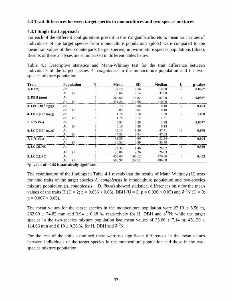
37

4.3 Trait differences between target species in monocultures and two-species mixtures

4.3.1 Single trait approach

For each of the different configurations present in the Yangambi arboretum, mean trait values of

individuals of the target species from monoculture populations (plots) were compared to the

mean trait values of their counterparts (target species) in two-mixture species populations (plots).

Results of these analyses are summarized in different tables below.

Table 4.1 Descriptive statistics and Mann-Whitney test for the trait difference between

individuals of the target species A. congolensis in the monoculture population and the two-

species mixture population

Trait Population N Mean SD Median U p-value

1. H (m) Ac 5 22.10 5.56 19.30 2 0.036*

Ac Dl 5 35.66 7.14 37.00

2. DBH (mm) Ac 5 262.60 74.82 287.00 2 0.036*

Ac Dl 5 451.20 114.66 410.00

3. LPC (10-2 mg/g) Ac 5 0.13 0.08 0.10 17 0.403

Ac Dl 5 0.09 0.02 0.10

4. LNC (10-2 mg/g) Ac 5 1.76 0.10 1.79 12 1.000

Ac Dl 5 1.78 0.12 1.81

5. δ15N (‰) Ac 5 3.94 0.28 3.98 0 0.007*

Ac Dl 5 6.18 0.38 6.13

6. LCC (10-2 mg/g) Ac 5 48.15 1.26 47.71 15 0.676

Ac Dl 5 47.55 0.94 47.63

7. δ13C (‰) Ac 5 -31.89 0.90 -32.24 4 0.094

Ac Dl 5 -30.52 0.99 -30.40

8. LCC:LNC Ac 5 27.35 1.46 28.02

16 0.530

Ac Dl 5 26.86 2.26 26.03

9. LCC:LPC Ac 5 455.60 166.12 470.06 8 0.403

Ac Dl 5 583.98 157.51 486.38

*p- value of <0.05 is statistically significant

The examination of the findings in Table 4.1 reveals that the results of Mann Whitney (U) tests

for nine traits of the target species A. congolensis in monoculture population and two-species

mixture population (A. congolensis + D. likwa) showed statistical differences only for the mean

values of the traits H (U = 2; p = 0.036 < 0.05), DBH (U = 2; p = 0.036 < 0.05) and δ15

N (U = 0;

p = 0.007 < 0.05).

The mean values for the target species in the monoculture population were 22.10 ± 5.56 m,

262.60 ± 74.82 mm and 3.94 ± 0.28 ‰ respectively for H, DBH and δ15

N; while the target

species in the two-species mixture population had mean values of 35.66 ± 7.14 m, 451.20 ±

114.66 mm and 6.18 ± 0.38 ‰ for H, DBH and δ15

N.

For the rest of the traits examined there were no significant differences in the mean values

between individuals of the target species in the monoculture population and those in the two-

species mixture population.

38

Table 4.2 Descriptive statistics and Mann-Whitney test for the trait difference between

individuals of the target species L. trichilioides in the monoculture population and the two-

species mixture population

Trait Population N Mean SD Median U p-value

1. H (m) Lt 5 17.74 9.99 14.80 7 0.296

Lt Ka 5 22.80 3.23 24.40

2. DBH (mm) Lt 5 168.00 38.35 159.00 7 0.296

Lt Ka 5 209.20 72.88 238.00

3. LPC (10-2 mg/g) Lt 5 0.09 0.01 0.10 7 0.296

Lt Ka 5 0.10 0.01 0.10

4. LNC (10-2 mg/g) Lt 5 2.91 0.13 2.89 25 0.007*

Lt Ka 5 2.47 0.02 2.47

5. δ15N (‰) Lt 5 7.36 0.35 7.43 25 0.007*

Lt Ka 5 4.18 0.63 4.03

6. LCC (10-2 mg/g) Lt 5 45.66 0.40 45.62 2 0.036*

Lt Ka 5 46.31 0.32 46.27

7. δ13C (‰) Lt 5 -31.19 0.92 -31.46 1 0.026*

Lt Ka 5 -29.17 1.01 -29.27

8. LCC:LNC Lt 5 15.69 0.71 15.71 0 0.007*

Lt Ka 5 18.70 0.29 18.68

9. LCC:LPC Lt 5 507.87 93.12 482.25 15 0.676

Lt Ka 5 467.24 24.99 463.16

*p- value of <0.05 is statistically significant

An examination of the findings in Table 4.2 shows that the results of the Mann Whitney U tests

applied to the nine traits examined for individuals of the target species L. trichilioides in the

monoculture population and in the two-species mixture population (L. trichilioides + K.

anthotheca) revealed statistically differences at level of p < 0.05 for the mean values of five

traits. These are LNC (U = 25; p = 0.007 < 0.05), δ15

N (U = 25; p = 0.007 < 0.05), LCC (U = 2;

p = 0.036 < 0.05), δ13

C ((U = 1; p = 0.026 < 0.05), LCC:LNC (U = 0; p = 0.007 < 0.05).

The compared mean values were respectively (2.91 ± 0.13) x 10-2

mg/g, 7.36 ± 0.35 ‰, (45.66 ±

0.40) x 10-2 mg/g, -31.19 ± 0.92 ‰ and 15.69 ± 0.71 for LNC, δ

15N, LCC, δ

13C, LCC:LNC in the

monoculture population, whereas in the two-species mixture population they were (2.47 ± 0.02)

x 10-2 mg/g, 4.18 ± 0.63 ‰, (46.31 ± 0.32) x 10

-2 mg/g, -29.17 ± 1.01 ‰ and 18.70 ± 0.29. These

mean values were higher for individuals of the target species in the monoculture population than

in the two species mixture population for the traits LNC and δ15

N. They were lower for for

individuals of the target species in the monoculture population than in the two species mixture

population for the traits LCC, δ13

C and LCC:LNC.

No significant differences in the mean values between individuals of the target species in the

monoculture population and those in the two-species mixture population were detected for all the

other traits.

39

Table 4.3 Descriptive statistics and Mann-Whitney test for the trait difference between

individuals of the target species M. africana in the monoculture population and the two-species

mixture population

Trait Population N Mean SD Median U p-value

1. H (m) Ma 5 32.04 8.85 36.60 10 0.676

Ma Sg 5 35.04 6.01 33.20

2. DBH (mm) Ma 5 387.00 167.18 343.00 7 0.296

Ma Sg 5 480.80 112.85 532.00

3. LPC (10-2 mg/g) Ma 5 0.07 0.01 0.07 6 0.210

Ma Sg 5 0.08 0.01 0.08

4. LNC (10-2 mg/g) Ma 5 1.75 0.11 1.72 19 0.210

Ma Sg 5 1.65 0.14 1.64

5. δ15N (‰) Ma 5 4.55 0.79 4.78 17 0.403

Ma Sg 5 4.42 1.49 4.13

6. LCC (10-2 mg/g) Ma 5 50.00 1.10 50.11 15 0.676

Ma Sg 5 49.50 0.22 49.57

7. δ13C (‰) Ma 5 -31.52 0.54 -31.47 5 0.143

Ma Sg 5 -31.05 0.56 -30.94

8. LCC:LNC Ma 5 28.73 1.58 28.97 7 0.296

Ma Sg 5 30.18 2.57 30.24

9. LCC:LPC Ma 5 786.18 143.71 752.58 20 0.153

Ma Sg 5 655.32 96.45 663.02

*p- value of <0.05 is statistically significant

The results of the Mann Whitney U tests in Table 4.3 indicate that there were no significant

differences between individuals of the target species M. africana in the monoculture population

and individuals of the same target species in the two species-mixture population (M. Africana +

S. grandifolia) for the mean values of all the traits examined at level of p < 0.05.

Table 4.4 Descriptive statistics and Mann-Whitney test for the trait difference between

individuals of the target species M.excelsa in the monoculture population and the two-species

mixture population

Trait Population N Mean SD Median U p-value

1. H (m) Me 5 32.60 8.79 28.40 16 0.531

Me Psp 5 28.46 5.83 30.90

2. DBH (mm) Me 5 278.00 49.12 290.00 5 0.144

Me Psp 5 420.80 150.58 409.00

3. LPC (10-2 mg/g) Me 5 0.13 0.01 0.13 25 0.007*

Me Psp 5 0.11 0.00 0.11

4. LNC (10-2 mg/g) Me 5 2.56 0.13 2.56 25 0.007*

Me Psp 5 2.37 0.00 2.37

5. δ15N (‰) Me 5 6.35 0.48 6.44 25 0.009*

Me Psp 5 4.92 0.00 4.92

6. LCC (10-2 mg/g) Me 5 43.18 0.72 43.21 1 0.022*

Me Psp 5 43.93 0.00 43.93

7. δ13C (‰) Me 5 -29.08 1.42 -29.47 10 0.666

Me Psp 5 -29.43 0.00 -29.43

8. LCC:LNC Me 5 16.86 0.58 16.86 0 0.007*

Me Psp 5 18.53 0.00 18.53

9. LCC:LPC Me 5 353.96 29.99 363.67 0 0.009*

Me Psp 5 409.79 0.00 409.79

*p- value of <0.05 is statistically significant

40

The results of the Mann Whitney U tests in Table 4.4 indicate that there were significant

differences at level of p < 0.05 between individuals of the target species M.excelsa in the

monoculture population and individuals of the same target species in the two species-mixture

population (M.excelsa + Phyllanthus sp.) for the mean values of the following traits: LPC (U =

25; p = 0.007 < 0.05), LCN (U = 25; p = 0.007 < 0.05), δ15

N (U = 25; p = 0.009 < 0.05), LCC (U

= 1; p = 0.022 < 0.05), C:N (U = 0; p = 0.007 < 0.05), LCC:LPC (U = 0; p = 0.007 < 0.05).

The mean trait values for individuals of the target species from the monoculture population were

higher than the mean trait values for individuals of the target species from the two species

mixture population for LPC: (0.13 ± 0.01) x 10-2 mg/g > (0.11 ± 0.00) x10

-2 mg/g; LNC: (2.56 ±

0.13) x 10-2 mg/g > (2.37 ± 0.00) x 10

-2 mg/g and δ15

N: (6.35 ± 0.48 ‰ > 4.92 ± 0.00 ‰). The

opposite was true for LCC: (43.18 ± 0.72) x 10-2

mg/g < (43.93 ± 0.00) x10-2

mg/g, LCC:LNC:

16.86 ± 0.58 < 18.53 ± 0.00) and LCC:LPC (353.96 ± 29.99 < 409.79 ± 0.00).

No significant differences in the mean values between individuals of the target species in the

monoculture population and those in the two-species mixture population were detected for the

remaining traits (H, DBH and δ13

C).

Table 4.5 Descriptive statistics and Mann-Whitney test for the trait difference between

individuals of the target species P. oleosa in the monoculture population and the two-species

mixture population

Trait Population N Mean SD Median U p-value

1. H (m) Po 5 20.50 10.51 19.00 7 0.296

Po Pe 5 28.82 3.04 29.88

2. DBH (mm) Po 5 279.00 146.05 286.00 8 0.403

Po Pe 5 344.40 64.69 355.00

3. LPC (10-2 mg/g) Po 5 0.11 0.01 0.11 12 1.000

Po Pe 5 0.13 0.05 0.11

4. LNC (10-2 mg/g) Po 5 3.08 0.21 3.09 5 0.144

Po Pe 5 3.29 0.03 3.29

5. δ15N (‰) Po 5 7.51 0.74 7.61 19 0.210

Po Pe 5 7.08 0.30 7.11

6. LCC (10-2 mg/g) Po 5 47.63 0.85 47.46 10 0.676

Po Pe 5 47.70 0.43 47.66

7. δ13C (‰) Po 5 -32.93 0.92 -32.75 13 1.000

Po Pe 5 -32.84 1.12 -33.08

8. LCC:LNC Po 5 15.50 0.97 15.23 21 0.095

Po Pe 5 14.45 0.24 14.41

9. LCC:LPC Po 5 421.33 47.33 451.95 14 0.834

Po Pe 5 428.19 131.11 437.71

*p- value of <0.05 is statistically significant

The results of the Mann Whitney U tests in Table 4.5 indicate that there were no significant

differences between individuals of the target species P. oleosa in the monoculture population and

individuals of the same target species in the two species-mixture population (P. oleosa + P.

elata) for the mean values of all the traits examined at level of p < 0.05.

41

Table 4.6 Descriptive statistics and Mann-Whitney test for the trait difference between

individuals of the target species P. soyauxii in the monoculture population and the two-species

mixture population

Trait Population N Mean SD Median U p-value

1. H (m) Ps 5 26.63 12.79 23.85 9 0.531

Ps Ta 5 29.80 2.73 29.30

2. DBH (mm) Ps 5 187.80 43.47 163.00 0 0.007*

Ps Ta 5 419.40 51.68 429.00

3. LPC (10-2 mg/g) Ps 5 0.10 0.01 0.10 5 0.143

Ps Ta 5 0.18 0.06 0.18

4. LNC (10-2 mg/g) Ps 5 3.20 0.33 3.22 9 0.531

Ps Ta 5 3.38 0.15 3.39

5. δ15N (‰) Ps 5 2.70 0.78 2.77 15 0.671

Ps Ta 5 2.62 0.83 2.60

6. LCC (10-2 mg/g) Ps 5 47.79 0.69 47.86 24 0.021*

Ps Ta 5 44.89 1.53 44.66

7. δ13C (‰) Ps 5 -31.53 0.49 -31.59 6 0.210

Ps Ta 5 -30.90 0.79 -31.15

8. LCC:LNC Ps 5 15.02 1.73 14.53 20 0.141

Ps Ta 5 13.43 1.05 13.46

9. LCC:LPC Ps 5 467.69 27.54 478.59 19 0.210

Ps Ta 5 374.13 125.51 385.75

*p- value of <0.05 is statistically significant

As revealed by the results of the Mann Whitney U tests in Table 4.6, there were significant

differences at level of p < 0.05 between individuals of the target species P. soyauxii in the

monoculture population and individuals of the same target species in the two species-mixture

population (P. soyauxii + T. africana) only for the mean values of two out of the nine trait

examined, namely DBH and LCC.

Individuals of the target species in the monoculture population had a lower DBH (Mean = 187.80

± 43.47 mm) compared to individuals of the same target species in the two-species mixture

population (Mean = 419.40 ± 51.68 mm), U = 0, p = 0.007 < 0.05. Individuals of the target

species in the monoculture population exhibited a higher LCC (Mean = (47.79 ± 0.69) x 10-2

mg/g) than those present in the two-species mixture population (Mean = (44.89 ± 1.53) x10-2

mg/g), U = 24, p = 0.021 < 0.05.

For the remaining seven traits examined, there were no significant differences in the mean values

between individuals of target species in the monoculture population and those in the two-species

mixture population.

42

Table 4.7 Descriptive statistics and Mann-Whitney test for the trait difference between

individuals of the target species P. tessmannii in the monoculture population and the two-species

mixture population

Trait Population N Mean SD Median U p-value

1. H(m) Pt 5 33.18 3.10 32.60 5 0.143

Pt Ca 5 38.36 8.09 38.93

2. DBH(mm) Pt 5 546.00 235.71 577.00 11 0.834

Pt Ca 5 624.20 360.56 546.00

3. LPC (10-2 mg/g) Pt 5 0.06 0.01 0.06 7 0.295

Pt Ca 5 0.09 0.05 0.06

4. LNC (10-2 mg/g) Pt 5 2.34 0.19 2.34 5 0.144

Pt Ca 5 2.64 0.27 2.68

5. δ15N (‰) Pt 5 2.08 0.92 1.98 4 0.0947

Pt Ca 5 3.12 0.56 3.07

6. LCC(10-2 mg/g) Pt 5 50.24 0.46 50.15 25 0.007*

Pt Ca 5 47.34 0.17 47.36

7. δ13C (‰) Pt 5 -30.32 0.89 -30.45 3 0.060

Pt Ca 5 -29.06 0.30 -29.11

8. LCC:LNC Pt 5 21.46 1.65 21.24 24 0.021*

Pt Ca 5 18.22 1.87 18.41

9. LCC:LPC Pt 5 840.01 96.06 844.06 19 0.021*

Pt Ca 5 567.56 160.55 576.82

*p- value of <0.05 is statistically significant

As shown by the results of Mann Whitney U tests set out in Table 4.7, the mean values of

individuals of the target species P. tessmannii in the monoculture population and those in the two

species-mixture population (P. tessmannii + Chrysophyllum africanum) were statistically

different at level of p < 0.05 for the traits LCC, LCC:LNC and LCC:LPC.

Individuals of the target species in the monoculture population had a higher LCC (Mean = (50.24

± 0.46) x 10-2 mg/g) compared to individuals of the same target species in the two-species

mixture population (Mean = (47.34 ± 0.17) x10-2 mg/g), U = 25, p = 0.007< 0.05. Similarly,

individuals of the target species in the monoculture population exhibited higher LCC:LNC and

LCC:LPC ratios (Mean = 21.46 ± 1.65 and Mean = 840.01 ± 96.06 respectively) than those

encountered in the two-species mixture population (Mean =18.22 ± 1.87 and Mean = 567.56 ±

160.55 respectively), U = 24, p = 0.02 < 0.05 for LCC:LNC and U = 19, p = 0.021 < 0.05 for

LCC:LPC.

The mean values of the individuals of the target species in the monoculture population and those

in the two-species mixture population did not show any statistical differences for the six

remaining traits investigated.

The results of the Mann Whitney U tests in Table 4.8 indicate that there were no significant

differences between individuals of the target species S. tetrandra in the monoculture population

and individuals of the same target species in the two species-mixture population (S. tetrandra +

P. elata) for the mean values of all the traits examined at level of p < 0.05.

43

Table 4.8 Descriptive statistics and Mann-Whitney test for the trait difference between

individuals of the target species S. tetrandra in the monoculture population and the two-species

mixture population

Trait Population N Mean SD Median U p-value

1. H(m) St 5 23.50 6.90 27.30 20 0.116

St Pe 5 17.50 3.67 15.40

2. DBH(mm) St 5 282.00 101.00 242.00 16 0.543

St Pe 5 256.00 82.13 214.00

3. LPC (10-2 mg/g) St 5 0.16 0.03 0.16 21 0.095

St Pe 5 0.12 0.03 0.11

4. LNC (10-2 mg/g) St 5 3.48 0.21 3.44 13 1.000

St Pe 5 3.47 0.44 3.58

5. δ 15 N (‰) St 5 6.77 0.97 6.93 14 0.834

St Pe 5 6.48 1.52 6.21

6. LCC(10-2 mg/g) St 5 48.60 0.64 48.30 12 1.000

St Pe 5 48.27 1.45 48.96

7. δ 13 C (‰) St 5 -35.29 0.43 -35.32 13 1.000

St Pe 5 -34.85 1.33 -35.69

8. LCC:LNC St 5 14.02 0.90 14.41 13 1.000

St Pe 5 14.08 1.56 13.71

9. LCC:LPC St 5 304.28 58.66 299.78 4 0.094

St Pe 5 424.07 109.71 448.59

*p- value of <0.05 is statistically significant

Table 4.9 Descriptive statistics and Kruskal Wallis test for the trait difference between

individuals of the target species E. cylindricum in the monoculture population and the two-

species mixture populations

Trait Population N Mean SD Median Mean

rank

K-W p-value

1. H (m) Ec 5 10.92 2.51 10.70 5.7 2.27 0.322

Ec An 5 18.70 12.78 10.80 8.4

Ec Ea 5 22.08 9.48 19.70 9.9

2. DBH (mm) Ec 5 160.60 71.37 146.00 5.4 2.54 0.281

Ec An 5 210.60 47.25 225.00 9.2

Ec Ea 5 201.40 44.34 220.00 9.4

3. LPC (10-2 mg/g) Ec 5 0.20 0.02 0.20 10.4a 9.38 0.009*

Ec An 5 0.21 0.03 0.20 10.6a

Ec Ea 5 0.12 0.01 0.12 3.0b

4. LNC (10-2 mg/g) Ec 5 3.51 0.00 3.51 3.0a 10.59 0.005*

Ec An 5 4.68 0.45 4.77 9.2ab

Ec Ea 5 5.13 0.31 5.06 11.8b

5. δ15N (‰) Ec 5 6.95 0.00 6.95 4.0a 10.28 0.006*

Ec Ea 5 7.53 0.68 7.59 7.2ab

Ec An 5 9.40 1.14 8.84 12.8b

6. LCC (10-2 mg/g) Ec An 5 43.90 1.01 43.80 4.0a 10.88 0.004*

Ec 5 45.02 0.00 45.02 7.0ab

Ec Ea 5 46.53 0.44 46.42 13b

7. δ13C (‰) Ec Ea 5 -30.19 0.42 -30.13 4.6 5.88 0.052

Ec 5 -29.81 0.00 -29.81 8.0

Ec An 5 -29.16 0.61 -29.10 11.4

8. LCC:LNC Ec 5 12.82 0.00 12.82 13.0a 9.97 0.007*

Ec An 5 9.58 1.00 9.76 6.2b

Ec Ea 5 9.12 0.63 9.18 4.8b

9. LCC:LPC Ec 5 183.28 0.00 183.28 4.0a 10.88 0.004*

Ec An 5 214.05 24.32 210.64 7.0ab

Ec Ea 5 413.44 28.62 407.54 13.0b

*p- value of <0.05 is statistically significant; Values within treatments for each analysis in the column Mean rank followed

by the same letter are not significantly different at p < 0.05 according to Dunn’s multiple range test.

44

The results of Kruskal Wallis tests in Table 4.9 indicate that there were significant differences

among individuals of the target species E. cylindricum present in the monoculture population,

those present in the first two-species mixture population (E. cylindricum + A. nannanii) and

those present in the second two-species mixture population (E. cylindricum + E. angolense) for

the mean values of six of the nine traits considered. These are LPC (K-W = 9.38; DF = 2; p =

0.009 < 0.05), LNC (K-W = 10.59; DF = 2; p = 0.005 < 0.05), δ15

N (K-W = 10.28; DF = 2; p =

0.006 < 0.05), LCC (K-W = 10.88; DF = 2; p = 0.004 < 0.05), LCC:LNC (K-W = 9.97; DF = 2;

p = 0.007 < 0.05) and LCC:LPC (K-W = 10.88; DF = 2; p = 0.004 < 0.05).

The multiple pairwise comparisons using Dunn’s procedure revealed that the LPC of individuals

of the target species in the monoculture population was statistically higher (Mean = (0.20 ± 0.02)

x 10-2 mg/g) than that of the individuals of the target species in the second two-species mixture

population (Mean = (0.12 ± 0.01) x 10-2 mg/g) but was not statistically different from the one of

individuals of the target species in the first two-species mixture population.

The same comparison procedure showed that the LNC of individuals of the target species in the

monoculture population was statistically lower (Mean = (3.51 ± 0.00) x 10-2 mg/g) than that of

individuals of the target species in the second two-species mixture population (Mean = (5.13 ±

0.31) x10-2 mg/g), but was not statistically different from the one of individuals of the target

species in the first two-species mixture population. In the case of the leaf trait δ15

N, a

significantly lower value was detected in leaves of individuals of the target species present in the

monoculture population (Mean= 6.95 ± 0.00 ‰) compared to leaves individuals of the target

species present in the first two-species mixture population (Mean = 9.40 ± 1.14 ‰).

For the LCC, individuals of the target species in the first two-species mixture population had a

statistically lower content (Mean = (43.90 ± 1.01 x 10-2 mg/g) than those in the second two

species-mixture population (Mean = (46.53 ± 0.44) x 10-2 mg/g). However, there were no

significant differences between the mean values of the individuals of the target species in the

monoculture population and those in both the first and second two-species mixture populations

for this trait.

The LCC:LNC ratio was statistically higher for individuals of the target species in the

monoculture population (Mean = 12.82 ± 0.00 ) than for individuals present in both the first two-

species mixture population (Mean = 9.58 ± 1.00) and the second two-species mixture population

(Mean = 9.12 ± 0.63). As for the LCC:LPC ratio, it was significantly lower for individuals of the

target species in the monoculture population (Mean = 183.28 ± 0.00) than for individuals present

in the second two-species mixture population (Mean = 413.44 ± 28.62).

For the remaining traits examined, there were no significant differences in the mean values

between individuals of the target species in the monoculture population and those in the first or

second two-species mixture populations.

45

Table 4.10 Descriptive statistics and Kruskal Wallis test for the trait difference between

individuals of the target species G.cedrata in the monoculture population and the two-species

mixture populations

Trait Population N Mean SD Median Mean

rank

K-W p-value

1. H (m) Gc 5 27.74 4.61 28.00 5.4 5.18 0.075

Gc Lt 5 34.64 1.41 35.12 11.6

Gc Pe 5 27.76 8.30 28.90 7.0

2. DBH (mm) Gc 5 223.00 71.53 213.00 4.5 4.62 0.099

Gc Lt 5 338.20 107.86 323.00 9.9

Gc Pe 5 307.80 54.43 337.00 9.6

3. LPC (10-2 mg/g) Gc 5 0.15 0.02 0.15 10.4 4.58 0.101

Gc Lt 5 0.12 0.01 0.12 4.6

Gc Pe 5 0.14 0.05 0.13 9.0

4. LNC (10-2 mg/g) Gc 5 3.33 0.30 3.41 7.2 3.23 0.198

Gc Lt 5 3.16 0.00 3.16 6.0

Gc Pe 5 3.64 0.39 3.76 10.8

5. δ15N (‰) Gc Lt 5 3.70 0.00 3.70 3.0a 10.14 0.006*

Gc Pe 5 8.16 0.38 8.18 9.6ab

Gc 5 8.46 1.41 8.99 11.4b

6. LCC (10-2 mg/g) Gc 5 48.14 1.13 48.29 7.4 0.39 0.821

Gc Lt 5 48.66 0.00 48.66 7.6

Gc Pe 5 48.22 0.99 48.04 9.0

7. δ13C (‰) Gc Lt 5 -31.60 0.00 -31.60 3.0a 10.16 0.006*

Gc 5 -31.11 0.59 -31.42 9.4ab

Gc Pe 5 -30.83 0.45 -31.02 11.6b

8. LCC:LNC Gc Pe 5 13.36 1.37 13.15 4.0a 6.62 0.036*

Gc 5 14.53 1.14 14.39 9.0ab

Gc Lt 5 15.39 0.00 15.39 11.0b

9. LCC:LPC Gc 5 333.52 44.97 337.75 5.0a 6.62 0.036*

Gc Pe 5 370.46 125.39 368.48 7.0ab

Gc Lt 5 460.79 0.00 460.79 12.0b

*p- value of <0.05 is statistically significant; Values within treatments for each analysis in the column Mean rank followed

by the same letter are not significantly different at p < 0.05 according to Dunn’s multiple range test.

As shown by the results of Kruskal Wallis tests in Table 4.10, there were significant differences

among individuals of the target species G.cedrata present in the monoculture population, those

present in the first two-species mixture population (G.cedrata + L. trichilioides) and those

present in the second two-species mixture population (G.cedrata + P. elata) for the mean values

of four out the nine traits measured. These are δ15

N (K-W = 10.14, DF = 2, p = 0.006 < 0.05),

δ13

C (K-W = 10.16, DF = 2, p = 0.006 < 0.05), LCC:LNC (K-W = 6.62, DF = 2, p = 0.036 <

0.05) and LCC:LPC (K-W = 6.62, DF = 2, p = 0.036 < 0.05).

The multiple pairwise comparisons using Dunn’s procedure showed that individuals of the target

species in the monoculture population had a significantly higher δ15

N value (Mean = 8.46 ± 1.41

‰) than the one of those in the first two-species mixture population (Mean = 3.70 ± 0.00 ‰).

The LCC:LPC ratio for the individuals of the target species in the monoculture population was

statistically lower (Mean = 333.52 ± 44.97) than the one for the individuals of the target species

in the first two-species mixture population (Mean = 460.79 ± 0.00).

There were no significant differences between the mean values of the individuals of the target

species in the monoculture population and those in both the first and second two-species mixture

46

populations for the traits δ13

C and LCC:LNC. Significant differences in the mean values were

rather detected between individuals of the target species present in the first and those in the

second two-species mixture populations.

For the remaining traits examined, there were no significant differences in the mean values

between individuals of the target species in the monoculture population and those in the first or

second two-species mixture populations.

Table 4.11 Descriptive statistics and Kruskal Wallis test for the trait difference between

individuals of the target species P. macrophylla in the monoculture population and the two-

species mixture populations

Trait Population N Mean SD Median Mean rank K-W p-value

1. H (m) Pm Cp 5 17.76 4.47 17.47 5.4a 8.66 0.013*

Pm 5 17.80 4.89 20.80 5.8a

Pm Zg 5 27.90 3.43 28.80 12.8b

2. DBH (mm) Pm 5 310.60 173.79 380.00 6.8 2.54 0.281

Pm Cp 5 461.20 103.15 443.00 10.6

Pm Zg 5 359.80 168.19 336.00 6.6

3. LPC (10-2 mg/g) Pm 5 0.10 0.00 0.10 7.5 0.40 0.818

Pm Cp 5 0.10 0.00 0.10 7.5

Pm Zg 5 0.12 0.03 0.13 9.0

4. LNC (10-2 mg/g) Pm 5 3.46 0.36 3.37 5.6 2.26 0.323

Pm Cp 5 3.63 0.00 3.63 9.0

Pm Zg 5 3.64 0.48 3.66 9.4

5. δ15N (‰) Pm 5 4.87 0.75 4.99 5.0a 9.85 0.007*

Pm Cp 5 5.29 0.00 5.29 6.0ab

Pm Zg 5 6.72 0.48 6.74 13.0b

6. LCC (10-2 mg/g) Pm 5 46.94 0.90 47.08 4.8a 6.97 0.031*

Pm Zg 5 47.34 0.29 47.28 7.2ab

Pm Cp 5 47.75 0.00 47.75 12b

7. δ13C (‰) Pm Cp 5 -32.65 0.00 -32.65 4.0a 7.55 0.023*

Pm 5 -31.29 1.64 -31.40 8.4ab

Pm Zg 5 -30.94 0.34 -30.88 11.6b

8. LCC:LNC Pm 5 13.78 1.21 14.11 10.4 2.26 0.323

Pm Cp 5 13.15 0.00 13.15 7.0

Pm Zg 5 13.01 1.90 12.87 6.6

9. LCC:LPC Pm 5 486.85 10.73 487.87 7.0 1.53 0.460

Pm Cp 5 494.82 0.00 494.82 10.0

Pm Zg 5 434.46 89.82 440.22 7.0

*p- value of <0.05 is statistically significant; Values within treatments for each analysis in the column Mean rank followed

by the same letter are not significantly different at p < 0.05 according to Dunn’s multiple range test.

An examination of the findings in the Table 4.11 indicates that that the results of the Kruskal

Wallis tests applied to the nine traits examined for the individuals of the target species P.

macrophylla in the monoculture population and in the two two-species mixture populations (P.

macrophylla + C. procera and P. macrophylla + Z. gilletii) revealed statistically differences at

level of p < 0.05 for the mean values of four traits. These are H (K-W = 8.66, DF = 2, p = 0.013

< 0.05), δ15

N (K-W = 9.85, DF = 2, p = 0.007 < 0.05), LCC (K-W = 6.97, DF = 2, p = 0.031 <

0.05) δ13

C (K-W = 7.55, D F= 2, p = 0.023 < 0.05).

As shown by the Dunn’s multiple pairwise comparisons, individuals of the target species in the

monoculture population were significantly shorter (Mean = 17.80 ± 4.89 m) and had a

statistically lower δ15

N value (Mean = 4.87 ± 0.75 ‰) than those in the two-species mixture

47

population composed of a combination of P. macrophylla and Z. gilletii (Mean = 27.90 ± 3.43 m

for H and Mean = 6.72 ± 0.48 ‰ for δ15

N).

In addition to that, individuals of the target species in the monoculture population exhibited a

significantly low LCC (Mean = (46.94 ± 0.90) x 10-2 mg/g) compared to the individuals of the

target species encountered in the two-species mixture population composed of a combination of

P. macrophylla and C. procera (Mean = (47.75 ± 0.00) x 10-2 mg/g).

Individuals of the target species in the monoculture population did not significantly differ from

the individuals of the target present in both two-species mixture population as far as the mean

values of the trait δ13

C was concerned. Instead, it is the individuals of target species present in

the first and second two-species mixture populations that significantly differed for the mean

values of this trait (δ13

C).

For the remaining traits examined, there were no significant differences in the mean values

between individuals of the target species in the monoculture population and those in the first or

second two-species mixture populations.

The results of Kruskal Wallis tests in Table 4.12 indicate that there was a significant difference

in the mean values among individuals of the target species P.elata present in the two

monoculture populations (plot No. 13 and No. 2) and those present in the four two-species

mixture populations (P.elata + G. cedrata; P.elata + B. welwitschii; P.elata + P. oleosa; P.elata

+ S. tetrandra) for the trait H (K-W =11.48, DF = 5, p = 0.043 < 0.05).

The multiple pairwise comparisons using Dunn’s procedure revealed a significant difference in

the height between individuals of the target species in the first monoculture populations (Plot

No.13) (Mean = 28.60 ± 6.91 m) and those in the two-species mixture population made of a

combination of P.elata + G. cedrata (Mean = 37.73 ± 0.39 m).

For the remaining traits examined, there were no significant differences in the mean values

between individuals of the target species in neither of the two monoculture populations and those

in the four two-species mixture populations.

48

Table 4.12 Descriptive statistics and Kruskal Wallis test for the trait difference between

individuals of the target species P.elata in the monoculture populations and the two-species

mixture populations

Trait Population N Mean SD Median Mean

rank

K-W p-value

1. H (m) Pe13 5 28.60 6.91 25.70 9.0a 11.48 0.043*

Pe2 5 32.52 1.95 32.00 11.2ab

Pe Bw 5 34.24 3.55 33.40 15.9ab

Pe Po 5 33.64 3.02 34.70 13.4ab

Pe St 5 34.24 5.30 35.90 17.6ab

Pe Gc 5 37.73 0.39 37.77 25.9b

2. DBH (mm) Pe13 5 279.40 52.92 279.00 10.0 2.7361 0.7406

Pe St 5 367.00 172.88 303.00 14.6

Pe2 5 352.00 85.48 335.00 16.5

Pe Bw 5 336.40 50.35 345.00 16.7

Pe Gc 5 425.40 222.85 409.00 17.4

Pe Po 5 365.80 86.78 344.00 17.8

3. LPC (10-2 mg/g) Pe Po 5 0.12 0.01 0.12 9.2 6.35 0.274

Pe2 5 0.13 0.01 0.13 13.8

Pe Bw 5 0.13 0.01 0.12 14.2

Pe Gc 5 0.13 0.02 0.13 15.8

Pe13 5 0.15 0.03 0.13 17.4

Pe St 5 0.15 0.02 0.15 22.6

4. LNC (10-2 mg/g) Pe13 5 4.20 0.15 4.21 9.2 6.44 0.266

Pe Gc 5 4.18 0.52 4.06 12.6

Pe Bw 5 4.35 0.21 4.30 14.6

Pe2 5 4.37 0.10 4.37 15.7

Pe Po 5 4.45 0.21 4.51 19.5

Pe St 5 4.60 0.33 4.48 21.4

5. δ15N (‰) Pe Gc 5 3.86 0.31 3.91 7.6 7.40 0.192

Pe13 5 4.27 0.84 4.20 14.2

Pe St 5 4.39 0.35 4.41 14.4

Pe Po 5 4.41 1.52 5.46 16.8

Pe2 5 4.66 0.24 4.69 18.1

Pe Bw 5 5.06 0.96 4.96 21.9

6. LCC (10-2 mg/g) Pe Gc 5 47.59 1.09 47.73 11.0 2.71 0.744

Pe St 5 47.88 0.51 48.04 13.0

Pe2 5 48.10 0.45 48.14 16.3

Pe13 5 48.20 1.60 48.18 16.4

Pe Bw 5 48.56 1.08 48.13 18.0

Pe Po 5 48.32 0.70 48.23 18.3

7. δ13C (‰) Pe13 5 -29.98 0.50 -30.01 7.8 11.22 0.05

Pe Gc 5 -30.12 1.61 -29.54 10.8

Pe Po 5 -29.43 0.29 -29.46 12.6

Pe Bw 5 -28.81 0.82 -28.64 18.6

Pe2 Pe2 5 -28.47 0.83 -28.54 21.4

Pe St 5 -28.54 1.22 -28.21 21.8

8. LCC:LNC Pe St 5 10.46 0.79 10.77 9.4 6.55 0.256

Pe Po 5 10.86 0.41 10.70 11.2

Pe2 5 11.01 0.26 10.89 15.2

Pe Bw 5 11.19 0.54 11.26 17.4

Pe Gc 5 11.51 1.26 12.07 18.60

Pe13 5 11.47 0.42 11.58 21.2

9. LCC:LPC Pe St 5 323.58 45.31 332.15 8.4 6.86 0.231

Pe13 5 342.33 69.17 364.08 14.4

Pe2 5 362.16 20.85 361.55 14.6

Pe Gc 5 366.47 63.81 375.96 15.2

Pe Bw 5 373.69 25.41 380.64 18.0

Pe Po 5 406.79 47.31 417.26 22.4

*p- value of <0.05 is statistically significant; Values within treatments for each analysis in the column Mean rank followed

by the same letter are not significantly different at p < 0.05 according to Dunn’s multiple range test.

49

The following highlights capture the key points of all the results presented and described above:

The interaction of the individuals of the admixed species D. likwa with those of the target

species A. congolensis in the mixture population led the latter to increase their size (H and DBH)

and as well as their δ15

N values in comparison with the monoculture population.

The interaction of individuals of the admixed species K. anthotheca with those of the target

species L. trichilioides in the mixture population made the latter to lower their LNC and their

δ15

N value whereas they increased their LCC, their δ13

C value and their LCC:LNC ratio value in

the mixture population compared to the monoculture population.

The interaction of the individuals of the admixed species Phyllanthus sp. with the individuals of

target species M.excelsa in the mixture population resulted in the decrease of LPC, LNC and that

of the δ15

N value of the target species in the mixture population compared to the monoculture

population. On the contrary, the LCC, LCC:LNC and LCC:LPC ratio values were increased.

The interaction of the individuals of the admixed species T. africana with the individuals of

target species P. soyauxii in the mixture population resulted in the increase of the target species

DBH and in the decrease of LCC of the target species in the mixture population as compared to

the monoculture population.

The interaction of the individuals of the admixed species C. africanum with those of the target

species P. tessmannii led to the decrease of the LCC of the target in the mixture population in

comparison to the monoculture population. The LCC:LNC and LCC:LPC ratios values of target

species were also decreased in the mixture population in comparison to the monoculture

population.

The interaction of the individuals of the admixed species A. nannanii with the individuals of

target species E. cylindricum in the mixture population resulted in an increase of the δ15

N value

and a decrease of the LCC:LNC ratio value of the target species in the mixture population in

comparison to the monoculture population.

The interaction of the individuals of the target species E. cylindricum with the individuals of the

admixed species E. angolense resulted in an increased LNC and an decreased LCC:LNC ratio

value for the target species in the mixture population when compared to monoculture population.

On the contrary, the LPC of the target species was lowered while its LCC:LPC ratio value was

augmented in the mixture population as compared to the monoculture population.

The interaction of the individuals of the admixed species L. trichilioides with those of the target

species G. cedrata induced a decrease in the δ15

N value of the target species while increasing its

LCC:LPC ratio value in the mixture population compared to the monoculture population.

The interaction of the individuals of the admixed species C. procera and the individuals of the

target species P. macrophylla made the latter to increase their LCC in the mixture population as

compared to the monoculture population.

50

The interaction of the individuals of the admixed species Z. gilletii with those of the target

species P. macrophylla resulted in an increased δ15

N value of the target species in the mixture

population as compared to the monoculture population. This interaction also induced an increase

in the H of the target species in the mixture population compared to the monoculture.

The interaction of the individuals of the admixed species G. cedrata with the individuals of

target species P. elata resulted in an increase in the H of the target species in the mixture

population compared to the second monoculture population (i.e plot No.13).

4.3.2 Multi-trait approach

The results of the between analysis tests for detecting the significance of grouping for the

BPCAs performed on each species are presented in Table 4.13.

Table 4.13 Between analysis tests for detecting the significance of grouping for the BPCAs

performed on each species

Population No. Perm. Obs. X < Obs. X ≥ Obs. P-value Ac 1000 2.86 995 5 < 0.005

Ac Dl

Ec 1000 5.94 1000 0 < 0.000

Ec An

Ec Ea

Gc 1000 3.35 991 9 < 0.009

Gc Lt

Gc Pe

Lt 1000 4.28 987 13 < 0.013

Lt Ka

Ma 1000 1.23 696 304 0.304ns

Ma Sg

Me 1000 4.26 990 10 <0.010

Me Psp

Pe2 1000 2.15 957 43 <0.043

Pe13

Pe Gc

Pe Bw

Pe Po

Pe St

Pm 1000 2.95 1000 0 <0.000

Pm Cp

Pm Zg

Po P 1000 1.34 764 236 0 .236ns

Po Pe

Ps 1000 2.99 983 17 <0.017

Ps Ta

Pt 1000 3.68 982 18 <0.018

Pt Ca

St 1000 1.12 618 382 0.382ns

St Pe

No. Perm= Number of permutations; Obs.= Observed value; X < Obs.= number of random values strictly

lower than the observed value; X ≥ Obs= number of random values strictly higher than the observed value,

p- value of <0.05 is statistically significant.

51

An examination of the findings in Table 4.13 shows that at significance level of 5 %, the nine

functional traits considered in the present study were able to significantly segregate the different

populations of target species (monocultures and two-species mixture populations) for nine out

twelve species examined (p-values ranging from <0.000 to <0.018).

The grouping of target species individuals in either the monoculture population or two-species

mixture population was not significant for the remaining three species, namely M. Africana (p =

0.304), P. oleosa (p = 0.236) and S. tetandra (p = 0.382).

For the grouping of target species with more than two populations (i.e. E. cylindricum, G.

cedrata, P. elata, P. macrophylla), additional between test analyses were performed to detect

whether the individuals in the monoculture populations could be significantly discriminated from

those in the two-species mixture populations. The results of these tests are summarized in table

4.14.

Table 4.14 Between analysis tests for detecting the segregation of monoculture populations from

two-species mixture populations for the grouping of target species with more than two

populations

Populations No. Perm. Obs. X < Obs. X ≥ Obs. P-value Ec vs. Ec/An 1000 4.12 998 2 < 0.002*

Ec vs. Ec/Ea 1000 5.85 999 1 <0.001*

Gc vs. Gc/Lt 1000 3.92 993 7 < 0.007*

Gc vs. Gc/Pe 1000 0.93 495 505 0.505ns

Pe2 vs. Pe/Bw 1000 0.48 140 860 0.860ns

Pe2 vs. Pe/Gc 1000 2.21 942 58 0.058ns

Pe2 vs. Pe/Po 1000 1.11 648 352 0.352ns

Pe2 vs. Pe/St 1000 1.48 855 145 0.145ns

Pe13 vs. Pe/Bw 1000 1.68 900 100 0.100ns

Pe13 vs. Pe/Gc 1000 0.99 597 403 0.403ns

Pe13 vs. Pe/Po 1000 2.17 960 40 0.040*

Pe13 vs. Pe/St 1000 1.73 916 84 0.084ns

Pe2 vs. Pe13 1000 1.98 949 51 0.051ns

Pm vs. Pm/Cp 1000 1.68 919 81 0.081ns

Pm vs. Pm/Zg 1000 2.081 983 17 <0.017*

No. Perm= Number of permutations; Obs.= Observed value; X < Obs.= number of random values strictly

lower than the observed value; X ≥ Obs= number of random values higher or equal than the observed value,

*p- value of <0.05 is statistically significant, ns= not significant.

These results in table 4.14 indicate that the nine functional traits taken together were able to

significantly segregate the individuals of the target species E. cylindricum present in the

monoculture population and those present in the first two-species mixture population composed

of E. cylindricum and A. nannanii (p < 0.002) on one hand, and those present in the second two-

species mixture population composed of E. cylindricum and E. angolensis (p < 0.001) on the

other hand.

Regarding the target species G. cedrata, the individuals in the monoculture population were

significantly discriminated from those in the first two-species mixture population constituted of

G.cedrata and L. trichilioides by the nine trait considered (p < 0.007), but not from those in the

second two-species mixture population constituted of G.cedrata and P. elata (p = 0.505).

52

The same pattern could also be recognized for the target species P. macrophylla whereby the

individuals constituting the monoculture population were significantly discriminated from those

making the two-species mixture population, P. macrophylla and Z. gilletii by the nine traits

considered (p < 0.017). However, the individuals belonging to the monoculture population could

not be significantly discriminated from the individuals constituting the two-species mixture

population, P. macrophylla and P. carapa by the traits considered (p = 0.081).

As for the target species P. elata, the individuals belonging to the first monoculture population

(plot No.2) did not significantly segregated from those in all the two-species mixture populations

in relation to the nine traits considered. The individuals in the second monoculture population

(plot No.13) could also not be discriminated from the individuals in the two-species mixture

populations by the nine traits considered, except for the individuals belonging to the two-species

mixture population made of P.elata and P.oleosa (p < 0.040). Additionally, there was no

significant discrimination between the individuals of the target species belonging to the first

monoculture population and those belonging to the second monoculture population (p = 0.051).

53

CHAPTER FIVE:

DISCUSSION

5.1. Variance partitioning

Part of the current study was concerned with knowing whether the majority of trait variation, for

the nine traits considered and across the twelve co-existing target species in the setup, was

situated within species or between species.

The variability within species (intra-specific) in the present study was higher than the variability

between species (inter-specific) for three of the nine traits considered, namely H and DBH and

LPC. For the above three mentioned traits, the intra-specific variability accounted for 69.08 %,

70.40 % and 73.98 % respectively of the overall variability when the single trait approach was

used whereas it accounted for 56.87 %, 64.97 % and 59.44 % respectively when the multi-trait

analysis taking into account the contribution of each of the nine variables (traits) was used.

At first sight, these results seem surprising considering the widely spread assumption that intra-

specific trait variation is negligible compared to variation among species (Garnier et al., 2001;

Baraloto et al., 2010; Auger and Shipley, 2013). However, studies where higher intra-specific

variations were measured in functional traits compared to inter-specific variations have already

been reported before.

Studying the variation in the functional traits LMA and LDMC across six nested ecological

scales, along a precipitation gradient for 119 tree species and 1910 leaves in lowland tropical

rainforests of East-West Panama, Messier et al. (2010) estimated the contribution of the intra-

specific variation to the overall variation for both traits at 48 % whereas the strictly inter-specific

variation fraction accounted for 21 % and 35 % respectively for LMA and LMDC. In their study

on variation in leaf functional trait values within and across individuals and species in a Costa

Rican dry forest, Hulshof and Swenson (2010) estimated the fraction of total variance within

species of 62 % and 68 % for the trait LWC when the leaves were collected at high (sun) and

low (shade) canopy positions, respectively.

These two studies that have reported a higher proportion of intra-specific variation relative to the

inter-specific variation for certain traits involved tree species in tropical forests as it is also the

case of the present study. However, a strong and valid generalization cannot be drawn only on

the basis of these few studies.

The intra-specific variability for the six remaining traits considered in the present study remained

lower than the inter-specific variability. However, except for the traits LNC and LCC:LNC, the

fraction of total variance within species for these traits was not marginal at all as it was

hypothesized at beginning of this study. It ranged from 23.29 % to 49.71 % when the single trait

approach was used and from 26.36 % to 38.33 % when the multi-trait analysis taking into

account the contribution of each of the nine variables (traits) was used. When the nine traits were

54

considered as a whole, the multi-trait variance decomposition resulted in fraction of 36.87 % for

the intra-specific variation against 63.13 % for inter-specific variation for the twelve species

studied. Using the same approach in a study involving thirteen herbaceous and shrub species and

the functional trait H, SLA, LDMC, LNC and LCC in the French Alps, Albert et al. (2010) also

noted a relatively strong component of intra-specific variability of about 30 % against 70 % for

the inter-specific component.

These results seem also to corroborate observations made previously that the fraction of total

variance between species relative to that within species is strongly dependent on the species and

traits considered. For instance, Wilson et al. (1999) noted that the intra-specific variability for

the trait SLA was about 8 % when all the plants of the considered dataset were incorporated into

the analysis. However, when only angiosperm species were taken into account in the analysis,

the fraction of total variance within species raised to 32 %. The same was true for the trait

LMDC for which the intra-specific variability increased from 6 % when all the plants were

considered to 14 % when only angiosperms were taken into account. As already stated by Albert

et al., (2010), it can be reaffirmed here that any decision seeking to know whether or not the

intra-specific variability can be neglected should be based on the system considered but also on

the selected trait and species.

A probable explanation for the fairly strong proportion of the intra-specific trait variation

obtained in this study could come from the fact that there might have been occurrence of biotic

interactions and niche complementarily between individuals of the target species at the

neighborhood scale. As explained by Violle et al. (2012), the appearance of biotic interactions

and niche complementarily at the neighborhood scale might force individuals of the same species

to adjust their trait values in response to the activity of their closest neighbor. As a result, the

relative importance of intra-specific trait variation to the overall trait variation is expected to

increase.

For the traits like δ15

N, LPC and H for which a fairly good fraction of between population

variation was observed, it can be assumed that this was as a result of the biotic interaction of the

target species with different admixed tree species to which were associated. The difference in the

species composition of different populations (plots) in this arboretum must have mediated a

relative higher between population variation in the particular case of the above mentioned traits.

5.2 Main functional trade-offs and strategies

The BPCA confirmed the well established leaf economics spectrum (Wright et al., 2004). In the

first dimension, species were separated according to their LCC and nutrient content (LPC and

LNC). Species with low nutrient content are expected to have thicker leaves. They are

characterized by a long life span and a slow return on investment. Species exhibiting high

nutrient content on the contrary are supposed to bear thinner leaves and are characterized by a

short life span and a fast return on investment. This illustrates well the acquisitive and

exploitative ecological strategies adopted by the species under investigation (Diaz et al., 2004).

55

In the second dimension, variations were mainly led by δ13

C, H, DBH. This reflects the strategies

utilize by these species in terms of water use efficiency, accessibility to light and investment in

perennial structures (Faster and Westoby, 2005). Plant H in particular has been mentioned as the

second main axis of variation in many previous studies (Diaz et al., 2004; Gross et al., 2007;

Albert et al., 2010).

The functional diversity exhibited by the considered species as portrayed by the BPCA axes

seems to suggest that within this planted tropical forest of Yangambi, target species co-exist with

diverse strategies that allow them to occupy different niches. However, the fact that a relatively

good number of the species investigated were situated around the centre of origin of the plane

(trait space) is an indication that they are characterized by an average values for the traits driving

the main axes variation in both the first and second dimension. Therefore, the co-existence of

these species in that arboretum may be explained by both the niche theory (Silvertown, 2004)

and the neutral theory (Hubblel, 2005).

The WPCA which focuses on axes that discriminate individuals within species in the trait space

seems to indicate that the main functional strategies adopted by the sampled species at the inter-

specific level were also maintained at the intra-specific level supporting the second hypothesis

made in this study. Though less marked, trait tradeoffs in terms of leaf economics and

accessibility to light and investment in perennial structures within species were broadly

analogous to that of between species.

Albert et al. (2010) in their study on herbaceous and shrub species in the French Alps made the

same observation that inter-specific functional strategies were broadly conserved at intra-specific

level. Maire et al. (2013) in a study among grass species involving two traits negatively

correlated along the LES (SLA and LLS) and two other negatively correlated traits (H and tiller

density: TD) but independent from the LES also indicated that that the trade-offs observed at the

inter-specific level were preserved at the intra-specific level as well. Contrary that these findings,

Boucher et al. (2013) in their study on the functional variability in the wild populations of the

herbaceous species Polygonum viviparum L. seemed to suggest that the main functional trade-

offs exhibited by plants at inter-specific level over large geographical scale could be different

from the ones at the population level.

5.3 Trait differences between target species in monocultures and two-species mixtures

5.3.1 Single trait approach

Using the single trait approach, significant differences in mean values for at least one trait (and

up to six traits) out of the nine traits examined were detected between individuals present in

monoculture populations and those in two-species mixture populations for nine species out of the

twelve sampled.

In the light of the results obtained from this part of the study, there seems to be phenotypic

plasticity for some of the studied traits in this planted tropical forest in line with the third

hypothesis of this work. Since it was the individuals of the same species occupying different

56

plots (i.e. belonging to different populations) that were each time compared, the trait differences

observed are presumably induced by changes in the growth environment rather than by genotype

differences.

The biotic interaction of some target species present in this arboretum with particular admixed

species might have led them to adjust their functional some of their functional trait values in

order to cope with the changing environmental conditions to which they were subjected. Because

the target species and their respective admixed species are native to the same region and co-exist

together, there is reason to believe that the new environmental conditions created by their

interaction were most probably driven by inter-specific competition for resources. The

availability of light, water and nutrients has been identified as the main cause responsible for

plant strategies in space and time (Ordonez, 2010).

Depending on the target species, the admixed species to which it was associated and the trait

involved, the mean trait value either increased or decreased in the mixture population compared

to the monoculture population. The traits that regularly showed a significant difference in the

mean values between individuals in different monoculture populations and those in two-species

mixture population were δ15

N, LCC and LCC:LNC. In their study on functional leaf trait

diversity of tree species in a Congolese secondary tropical forest, Verbeeck et al. (2014) had also

noted that the leaf trait δ15

N was strongly influenced by plot location.

In the case of this study, a pattern seemed to emerge throughout different configurations of the

arboretum pointing out an interplay between the LCC and LNC and its isotope δ15

N. Whenever

the interaction of an admixed species with a target species led to an increase in the LNC and/or

the δ15

N value in the mixture population in comparison to the monoculture population, the LCC

value was almost always lowered and vice-versa. This could be as a result of the competition

from the admixed species on the target species for N, water or light resulting, perhaps, in a

divergent allocation of C and N within the leaves of the target species in the mixture populations

in comparison to those in monoculture populations.

N is considered as one of the most important nutrients steering plant composition and richness,

and plants need C as source of energy for their growth (biomass accumulation). The C economy

and the N economy are known to be closely linked. It has been demonstrated for instance that

plants allocate more biomass to roots versus leaves and increase their N concentration when

water is in short supply (Ye et al., 2015). It is also known that in low light environments, plants

exhibit higher leaf-to-root ratios and lower their N content than in high light environments

(Suguira and Tateno, 2011). In a similar way, fast growing plant species are believed to allocate

more biomass to the roots in suboptimal N supply conditions (Aerts and chapin, 2000).

The observed interplay of LCC and LNC in target species as a result of their interaction with

admixed species seems also to be a good illustration of how phenotypic plasticity may lead to

niche differentiation, thus avoiding competitive exclusion. Through phenotypic plasticity,

organisms are able to adjust to an array of conditions without evolutionary changes. Siefert

(2012) explained that apart from genetic variation, phenotypic plasticity could also make

57

species’ trait values to differ among locations as response to environmental filters and interaction

with neighboring species. Niche differentiation among species can be interpreted as the capacity

of species to exploit diverse environments, and it is sometimes expressed as changes in species

performance (Roscher et al., 2015). It has been identified as one of the main factors driving

species co-existence (Levine et al., 2009).

The interaction of the individuals of the target species M. Africana, P. oleosa and S. tetandra

with their respective admixed species resulted in no significant difference in the mean values of

all the traits examined between the individuals of these target species in monoculture populations

and those in mixture populations. A plausible explanation to that could come from the neutral

theory. It states that co-existing species are functionally the same; therefore, they share similar

niches (Hubbell, 2005). The interaction of the individuals of the above mentioned target species

with their respective admixed species did probably not lead to any change in their respective

environmental conditions. Therefore, there was no reason for them to differ from their

counterparts in monoculture populations with respect to the considered functional traits.

5.3.2 Multi-trait approach

Another interesting lesson learnt from the results of this study came from multi-trait analyses that

were used to test the significance of grouping for the BPCAs performed on each species. The

results of these tests suggest that the nine functional traits used in this study significantly

segregated the different monoculture populations from the mixture populations for nine target

species out of the twelve tested. This also implies that the individuals of the different populations

that were compared were significantly different in terms of the considered functional traits.

The three target species for which the monoculture populations could not be significantly

segregated from the mixture population were M. africana, P. oleosa and S. tetandra. These

results were consistent with those obtained when the single trait analyses were used. They seem

to suggest that a difference in a single trait between a monoculture population and a mixture

population for a particular target species was enough to make the two groups different when the

nine traits were considered together. Since many plant functional traits tend to co-vary together,

it is quite possible that a plastic response of single trait to changing environmental conditions

could also impact functionally correlated traits when a suite of traits are considered together

(Roscher et al., 2015). Therefore, co-variations among species traits could be playing an

important role in the overall performance of plants.

58

CHAPTER SIX:

GENERAL CONCLUSION AND RECOMMENDATIONS

6.1 General conclusion

The variance decomposition performed in this study showed that the inter-specific variation

dominated for all the traits examined except for the trait DBH and H and LPC. Despite this fact,

the intra-specific variation was not negligible. The overall partition taking into account the nine

functional traits and twelve species studied together was estimated at 36.87 % for the intra-

specific variation against 63.13 % for inter-specific variation. This fairly good proportion of

intra-specific variation vs. inter-specific variation can be attributed the appearance of biotic

interactions and niche complementarily at the neighborhood scale between individuals of the

same species. The consequence of this is an increase in the relative importance of intra-specific

variation. These results point to the importance of incorporating intra-specific trait variation into

community assembly analyses.

The functional dimensions identified in this study were in accordance with the well known leaf

economy spectrum. Species were segregated depending on the LCC, LNC and LPC in the first

dimension. In the second axis, variation was led by δ13

C, H, DBH. It was also shown that the

main functional strategies adopted by the investigated species at the inter-specific level were also

maintained at the intra-specific level.

Using single trait-analyses, significant differences in trait values were detected between target

species in monocultures and in two-species mixtures for nine species out of the twelve

investigated. An apparent interplay between the traits δ15

N, LNC and LCC was recognized

throughout different configurations of the arboretum. An increase in LNC and/or δ15

N value in

the mixture population of a specific target species due the interaction of its individuals with those

of the admixed species was almost always followed by a reduction in the LCC and vice versa.

This tends to indicate the occurrence of phenotypic plasticity among the individuals of the target

species in the mixture populations as a result of their competition with their respective admixed

species allowing a divergent allocation of C and N within their respective leaves. The occurrence

of this phenotypic plasticity was probably responsible for the niche differentiation explaining the

co-existence of these target species with the admixed species which they were associated to.

For three target species, namely M. africana, P. oleosa and S. tetandra, no significant differences

in trait values were detected between individuals in monocultures and those in two-species

mixtures for all the nine traits examined. Most probably the interaction of these target species

with their respective admixed species resulted in no major inter-specific competition for

resources. Hence, the neutral theory was proposed as the possible cause explaining the co-

existence of these target species with the respective admixed species with which they were

combined.

59

The results of the multi-trait analyses that were used to test if the nine functional traits taken

together could significantly differentiate between the monoculture populations and mixture

populations of the target species were in line with the results obtained from the single trait

analyses. It was found that a difference in a single trait between a monoculture population and a

mixture population for a particular target species as detected through the single trait analysis was

enough to make the two groups different when the nine traits were considered together.

Altogether this study has shown how intra-specific variation was mediating the co-existence of

target species in this arboretum by accounting for good proportion of the total variation for most

traits, by maintaining the same functional trade-offs and strategies at the intra-specific level and

at the inter-specific level, and through the occurrence of phenotypic plasticity.

These results have highlighted the important role that the intra-specific trait variation may play in

determining tree species co-existence. Therefore, the intra-specific trait variation should not be

systematically neglected in quantitative functional trait-based analyses. The decision on whether

or not to neglect the intra-specific trait variation should be made on a case-by-case basis taking

into account the trait, the species and the system under investigation.

6.2. Recommendations

To be complete and to confirm some of the outcomes of this study, these investigations should

be extended to the admixed species. It will be of particular importance to compare the trait

values of the target species in monoculture populations and in mixture populations with those of

the admixed species in mixture populations. In addition, studies on nutrient cycling and the

pattern of C and N allocation to roots and leaves of the species in the arboretum will also be

needed. This will allow elucidating further the role of inter-specific competition between the

target species and admixed species as a probable cause of the observed variation in the trait

values of the target species in monoculture populations and mixture populations.

60

REFERENCES

Ackerly, D. D., Dudley, S. A., Sultan, S. E., Schmitt, J., Coleman, J. S., Linder, R., Sandquist,

D. R., Geber, M. A., Evans, A. S., Dawson, T. E., Lechowicz M. J. 2000. The evolution of

plant ecophysiological traits: recent advances and future directions. Bioscience 50:979-995.

Aerts, R. and Chapin, F. S. 2000. The mineral nutrition of wild plants revisited: a re-evaluation

of processes and patterns. Advance in Ecological Research 30: 1-67.

Albert C. H., Grassein F., Schurr F. M., Vieilledent G. and Violle C. 2011. When and how

should intraspecific variability be considered in trait-based plant ecology? Perspectives in

Plant Ecology, Evolution and Systematics 13:217-225.

Albert, C. H., Thuiller, W., Yoccoz, N. G., Douzet, R., Aubert, S. and Lavorel, S. 2010. A multi-

trait approach reveals the structure and the relative importance of intra- vs. interspecific

variability in plant traits. Functional Ecology 24:1192-1201.

Alcoverro, T., Manzanera, M. and Romero, J. 2000. Nutrient mass balance of the sea grass

Posidonia oceanica: the importance of nutrient retranslocation. Marine Ecology Progress

Series 194: 13-21

Arndt, S. K and Wanek, W. 2002. Use of decreasing foliar carbon isotope discrimination during

water limitation as a carbon tracer to study whole plant carbon allocation. Plant, Cell and

Environment 25: 609-616.

Auger, S. and Shipley, B. 2013. Inter-specific and intra-specific trait variation along short

environmental gradients in an old-growth. Journal of Vegetation Science 24: 419-428.

Badyaev, A. V. 2009. Evolutionary significance of phenotypic accommodation in novel

environments: an empirical test of the Baldwin effect. Philosophical Transactions of the

Royal Society B 364:1125-1141.

Baker, T. R., Phillips, O. L., Malhi, Y., Almeida, S., Arroyo, L. Arroyo, L., Di Fiore, A.,

Killeen, T. J., Laurance, S. G., Laurance, W. F., Lewis, S. L., Lloyd, J., Monteagudo, A.,

Neill, D. A., Patino, S., Pitman, N. C. A., Macedo Silva, J. N. and Vasquez Martinez, R.

2004. Variation in wood density determines spatial patterns in Amazonian forest biomass.

Global Change Biology 10:545-562.

Baraloto, C., Hardy, O.J., Paine, C. E. T., Dexter, K. G., Cruaud, C., Dunning, L. T., Gonzalez,

M., Molino, J., Sabatier, D., Savolainen, V. and Chave, J. 2012. Using functional traits and

phylogenetic trees to examine the assembly of tropical forest tree communities. Journal of

Ecology 100:690-701.

Baraloto, C., Paine, C. E. T., Poorter, L., Beauchene, J., Bonal, D., Domenach, A. M., Hérault,

B., Patiño, S., Roggy, J. C. and Chave, J. 2010. Decoupled leaf and stem economics in rain

forest trees. Ecology Letters 13: 1338-1347.

Bazzaz, F. A. and Pickett, S. T. A. 1980. Physiological ecology of tropical succession: A

comparative review. Annual Review of Ecology and Systematics 11:287-310.

61

Bolnick, D. I., Amarasekare, P., Araújo, M. S., Bürger, R., Levine, J. M., Novak, M., Rudolf, V.

H. W., Schreiber, S. J., Urban, M. C., Vasseur, D. A. 2011. Why intra-specific trait

variation matters in community ecology. Trends in Ecology and Evolution 26(4):183-192.

Bonan, G. B. 2008. Forests and climate change: forcings, feedbacks, and the climate benefits of

forests. Science 320:1444-1449.

Boucher, F. C., Thuiller, W., Arnoldi, C., Albert, C. H and Lavergne, S. 2013. Unravelling the

architecture of functional variability in wild populations of Polygonum viviparum L.

Functional Ecology 27: 382-391.

Boyemba, B.F. 2011. Ecologie de Pericopsis elata (Harms) Van Meeuwen (Fabaceae), arbre de

forêt tropicale africaine à répartition agrégée. PhD thesis, Université Libre de Bruxelles,

Bruxelles, 181p.

Butler, R. 2014. Tropical rainforest of the world. www. rainforest.mongabay.com, retrieved on

24.07.2015

Carvalho, J. A., Higuchi, N., Araújo, T. M and Santos, J. C. 1998. Combustion completeness in a

rainforest clearing experiment in Manaus, Brazil. Journal of geophysical research 103:

13195-13199.

Cattanio, J. H., Kuehne, R. and Vlek, P. L. 2008. Organic material decomposition and nutrient

dynamics in a mulch system enriched with leguminous trees in the amazon. The Revista

Brasileira de Ciência do Solo32:1073-1086.

Chapman, H. D. and Pratt, F. P. 1961. Ammonium Vandate-molybdate method for determination

of phosphorus: Methods of analysis for soils, plants and water. 1st edition, Agriculture

Division, California University, USA, pp. 184-203.

Chave, J., Coomes, D., Jansen, S., Lewis, S. L., Swenson, N. G. and Zanne, A. E. 2009. Towards

a worldwide wood economics spectrum. Ecology Letters 12:351-366.

Clark, J. S., Bell, D., Chu, C., Courbaud, B., Dietze, M., Hersh, M., HilleRisLambers, J., Ibáñez,

I., LaDeau, S., McMahon, S., Metcalf, J., Mohan, J., Moran, E., Pangle, L., Pearson, S.,

Salk, C., Shen, Z., Valle, D. and Wyckoff, P. 2010. High-dimensional coexistence based on

individual variation: a synthesis of evidence. Ecological Monographs 80:569-608

Cornelissen, J. H. C., Lavorel, S., Garnier, E., Díaz, S., Buchmann, N., Gurvich, D. E., Reich, P.

B., ter Steege, H., Morgan, H. D, van der Heijden, M.G.A, Pausas, J. G.and Poorter, H.

2003. A handbook of protocols for standarised and easy measurement of plant functional

traits worldwide. Australian Journal of Botany 51:335-380.

Cornwell, W. K. and Ackerly, D. D. 2009. Community assembly and shifts in plant trait

distributions across an environmental gradient in coastal California. Ecological

Monographs 79:109-126.

Dale, V. H., Joyce, L. A., McNulty, S., Neilson, R. P., Ayres, M. P., Flanningan, M. D., Hanson,

P. J., Irland, L. C., Lugo, A. E., Peterson, C. J., Simberloff, D., Swanson, F. J., Stocks, B. J.

and Wotto, B. M. 2001. Climate change and forest disturbances. BioScience 51:723-34

62

de Bello, F., Lavorel, S., Albert, C.H., Thuiller, W., Grigulis, K., Dolezal, J., Janecek, S. and

Leps, J. 2011. Quantifying the relevance of intraspecific trait variability for functional

diversity. Methods in Ecology and Evolution 2: 163-174.

Díaz, S. and Cabido, W. 2001. Vive la différence: plant functional diversity matters to ecosystem

processes. Trends in Ecology and Evolution 16(11):646-655.

Diaz, S., Hodgson, J. G., Thompson, K., Cabido, M., Cornelissen, J. H. C., Jalili, A., Montserrat

Marti, G., Grime, J. P., Zarrinkamar, F., Asri, Y., Band, S. R., Basconcelo, S., Castro-Diez,

P., Funes, G., Hamzehee, B., Khoshnevi, M., Perez-Harguindeguy, N., Perez-Rontome,

M.C., Shirvany, F. A., Vendramini, F., Yazdani, S., Abbas-Azimi, R., Bogaard,A.,

Boustani, S., Charles, M., Dehghan, M., De Torres-Espuny, L., Falczuk, V.,Guerrero-

Campo, J., Hynd, A., Jones, G., Kowsary, E., Kazemi-Saeed, F., Maestro- Martinez, M.,

Romo-Diez, A., Shaw, S., Siavash, B., Villar-Salvador, P. and Zak,M. R. 2004. The plant

traits that drive ecosystems: evidence from three continents. Journal of Vegetation Science

15: 295-304.

Dodélec, S. and Chessel, D. 1991. Recent developments in linear ordination methods for

environmental sciences. Advances in Ecology, India, 1: 133-155.

Ernst, C., Mayaux, P., Verhegghen, A., Bodart, C., Musampa, C. and Defourny, P. 2013.

National forest cover change in Congo Basin: deforestation, reforestation, degradation and

regeneration for the years 1990, 2000 and 2005. Global Change Biology 19:1173-1187.

Falster, D. S. and Westoby, M. 2005. Alternative height strategies among 45 dicot rain forest

species from tropical Queensland, Australia. Journal of Ecology 93:521-535.

FAO. 2010. Global forest resources assessment 2010. Forestry paper 163, FAO, Rome. 340p.

Fichman, M. and Cummings, J. M. 2003. Multiple imputation for missing data: Making the most

of what you know. Organizational Research Methods 6(3):282-308.

Field, C., and Mooney, H. A. 1986.The photosynthesis-nitrogen relationship in wild plants. In:

On the economy of plant form and function: adaptative patterns of energy capture in

plants. (T. J. Givnish, ed.), pp. 25-56, Cambridge University Press, Cambridge.

Fonseca, C. R., Overton, J. M., Collins, B. and Westoby, M. 2000. Shifts in trait combinations

along rainfall and phosphorous gradients. Journal of Ecology 88:964-977.

Fortunel, C., Garnier, E., Joffre, R., Kazakou, E., Quested, H., Grigulis, K., Lavorel, S., Ansquer,

P., Castro, H., Cruz, P., Dolezal, J., Eriksson, O, Freitas, H., Golodets, C., Jouany, C,

Kigel, J, Kleyer, M., Lehsten, V, Leps, J, Meier, T., Pakeman, R., Papadimitriou, M.,

Papanastasis, V. P., Quétier F., Robson, M., Sternberg, M., Theau, J.P., Thébault, A. and

Zarovali, M. 2009. Leaf traits capture the effects of land use changes and climate on litter

decomposability of grasslands across Europe. Ecology 90 (3): 598-611.

Franklin, J. F., Spies, T. A., Van Pelt, R., Carey, A. B., Thornburgh, D.A., et al., 2002.

Disturbances and structural development of natural forest ecosystems with silvicultural

implications, using Douglas fir forests as an example. Forest Ecology and Management

155:399-423

63

Fridley, J. D., Grime, J. P. and Bilton, M. 2007. Genetic identity of interspecific neighbours

mediates plant responses to competition and environmental variation in a species-rich

grassland. Journal of Ecology 95:908-915.

Gadow, K., Zhang, C. Y., Wehenkel, C., Pommerening, A., Corral-Rivas, J., Korol, M.,

Myklush, S., Hui, G. Y., Kiviste, A. and Zhao, X. H. 2012. Forest structure and diversity.

Managing Forest Ecosystems 23:29-83.

Garnier, E., Cordonnier, P., Guillerm, J. L. and Sonié, L. 1997. Specific leaf area and leaf

nitrogen concentration in annual and perennial grass species growing in Mediterranean old-

fields. Oecologia, 111: 490-498.

Garnier, E., Laurent, G., Bellmann, A., Debain, S., Berthelier, P., Ducout, B., Roumet, C., Navas

and M. L. 2001. Consistency of species ranking based on functional leaf traits. New

Phytologist 152: 69-83.

Gibbs, H. K., Brown, S., Niles, J. O. and Foley, J. A. 2007. Monitoring and estimating tropical

forest carbon stocks: making REDD a reality. Environmental Research Letters 2(4):054023

Giller, K.E. 2001. Nitrogen fixation in tropical cropping systems, 2nd

edition, CABI Publising,

Wallingford, UK. 423p.

Grime, J. P. and Pierce, S. 2012. The evolutionary strategies that shape ecosystems. Wiley-

Blackwell, Chichester, UK. 244p.

Grime, J. P., Thompson, K., Hunt, R., Hodgson, J. G., Cornelissen, J. H. C., Riorison, I. H.,

Hendry, G. A .F., Ashenden, T. W., Askew, A. P., Band, S. R., Booth, R. E., Bossard, C.

C., Campbell, B. D, Cooper, J.E., Davison, A. W., Gupta, P. L., Hall, W., Hand, D. W,

Hannah, M. A., Hillier, S. H., Hodkinson, D. J., Jalili, A., Liu, Z., Mackey, J. M. L.,

Matthews, N., Mowforth, M. A., Neal, R. J., Reader, R. J., Reiling, K., Ross-Fraser, W.,

Spencer, R. E., Sutton, F., Tasker, D. E., Thorpe, P. C. and Whitehouse, J. 1997. Integrated

screening validates primary axes of specialization in plants. 1997. Integrated screening

validates primary axes of specialization in plants. Oikos 79: 259-281.

Gross, N., Suding, K. N., Lavorel, S. and Roumet, C. 2007. Complementarity as a mechanism of

coexistence between functional groups of grasses. Journal of Ecology 95: 1296-1305.

Güsewell, S. 2004. N : P ratios in terrestrial plants: variation and functional significance. New

Phytologist 164(2): 243-266.

Hubbell, S. P. 2005. Neutral theory in community ecology and the hypothesis of functional

equivalence. Functional Ecology 19(1):166-172.

Hughes, A. R. and Stachowicz. J. J. 2004. Genetic diversity enhances the resistance of a seagrass

ecosystem to disturbance. Proceedings of the National Academy of Sciences USA

101:8998-9002.

Hulshof, C. M. and Swenson, N. G. 2010. Variation in leaf functional trait values within and

across individuals and species: an example from a Costa Rican dry forest. Functional

Ecology 24: 217-223.

64

IPCC, 2007. Climate Change 2007: Impacts, Adaptation and Vulnerability: Contribution of

Working Group II to the Fourth Assessment Report of the Intergovernmental Panel on

Climate Change. Cambridge University Press, Cambridge, United Kingdom and New

York, NY, USA. 976p.

Jung, V., Violle, C., Mondy, C., Hoffmann, L. and Muller, S. 2010. Intraspecific variability and

trait-based community assembly. Journal of Ecology 98:1134-1140.

Kang, M., Chang, S. X., Yan, E-R. and Wang, X-H. 2014. Trait variability differs between leaf

and wood tissues across ecological scales in subtropical forests. Journal of Vegetation

Science 25: 703-714.

Kooyman, R. M. and Westoby, M. 2009. Costs of height gain in rainforest saplings: main-stem

scaling, functional traits and strategy variation across 75 species. Annals of Botany

104:987-993

Kotowska, A. M., Cahill, J. F. and Keddie., B. A. 2010. Plant genetic diversity yields increased

plant productivity and herbivore performance. Journal of Ecology 98:237-245.

Kraft, N. J. B., Valencia, R. and Ackerly, D. D. 2008. Functional traits and niche-based tree

community assembly in an Amazonian forest. Science 322:580-582.

Krieger, D. 2001. Economic value of forest ecosystem services: A review. The Wilderness

Society, Washington, D.C. 31p.

Laughlin, D. C. 2014. The intrinsic dimensionality of plant traits and its relevance to community

assembly. Journal of Ecology 102:186-193.

Lee, J.A. and Verleyson, M. 2007. Nonlinear Dimensionality Reduction. Springer, New York,

NY. 309p.

Levine, J. M., Hille Ris Lambers, J. 2009. The importance of niches for the maintenance of

species diversity. Nature 461: 254-257.

Linhart, Y. B. and Grant, M. C. 1996. Evolutionary significance of local genetic differentiation

in plants. Annual Review of Ecology and Systematics 27:237-277.

Liu, J., Zeng, D., Lee, D. K., Fan, Z. and Zhong, L. 2008. Leaf traits and their interrelationship

of 23 plant species in southeast of Keerqin Sandy Lands, China. Frontiers of Biology in

China 3: 332-337.

Lloyd, J., Bloomfield, K., Domingues, T. F. and Farquhar, G. D. 2013. Photosynthetically

relevant foliar traits correlating better on a mass vs an area basis: of ecophysiological

relevance or just a case of mathematical imperatives and statistical quicksand? New

Phytologist 199:311-321.

Maire, V., Gross, N., Hill, D., Martin, R., Wirth, C., Wright, I. J and Soussana, I. J. 2013.

Disentangling coordination among functional traits using anindividual-centred model:

Impact on plant performance at intra- and inter-specific levels. PLoS ONE 8(10): e77372.

doi:10.1371/journal.pone.0077372.

65

Marthews, T. R., Metcalfe, D., Malhi, Y., Phillips, O., Huaraca, H. W., Riutta, T., Ruiz, J.

M.,Girardin, C., Urrutia, R., Butt, N., Cain, R., Oliveras, M. I and colleagues from the

RAINFOR and GEM networks. 2012. Measuring tropical forest carbon allocation and

cycling: A RAINFOR-GEM field manual for intensive census plots (v2.2). Manual, Global

Ecosystems Monitoring network, http://gem.tropicalforests.ox.ac.uk/

McGroddy, M. E., Daufresne, T. and Hedin, L. O. 2004. Scaling of C : N : P stoichiometry in

forests worldwide: implications of terrestrial Redfield-type ratios. Ecology 85(9): 2390-

2401.

MECNT, DRC/UN-REDD. 2012. Synthèse des études sur les causes de la déforestation et de la

dégradation des forêts en République Démocratique du Congo, Version Finale. MECNT,

Kinshasa. 40p.

Mediavilla, S. and Escudero, A. 2003. Leaf life span differs from retention time of biomass and

nutrients in the crowns of evergreen species. Functional Ecology 17: 541-548.

Meir, P., Kruijt, B., Broadmeadow, M., Barbosa, E., Kull, O., Carswell, F., Nobre, A. and

Jarvis, P.G. 2002. Acclimation of photosynthetic capacity to irradiance in tree canopies in

relation to leaf nitrogen concentration and leaf mass per unit area. Plant Cell Environment

25:343-357.

MENCT, RDC. 2009. The Democratic Republic of Congo’s REDD+ Potential. MENCT,

Kinshasa. 62p.

Messier, J., McGill, B. J. and Lechowicz, M. J. 2010. How do traits vary across ecological

scales? A case for trait-based ecology. Ecology Letters 13:838-848.

Miner, B. G., Sultan S. E, Morgan, S. G., Padilla, D. K., Relyea, R. A. 2005. Ecological

consequences of phenotypic plasticity. Trends in Ecology and Evolution 20(12):685-692.

Moreira, B., Tavsanoglu , Ç. and Pausas, J. G. 2012. Local versus regional intraspecific

variability in regeneration traits. Oecologia 168:671-677.

Ngongo, M. L., van Ranst, E., Baert, G., Kasongo, E. L., Verdoodt, A., Mujinya, B. B. and

Mukalay, J. M. 2009. Guide des sols en R.D. Congo. Tome I: Etude et Gestion. UGent -

HoGent-UNILU, 262 p.

Onoda, Y., Richards, A. E. and Westoby, M. 2010. The relationship between stem biomechanics

and wood density is modified by rainfall in 32 Australian woody plant species. New

Phytologist 185:493-501.

Ordonez, J. C., van Bodegom, P. M., Witte, J. P. M., Bartholomeus, R. P., van Hal, J. R., Aerts,

R. 2010. Plant strategies in relation to resource supply in mesic to wet environments: Does

theory mirror nature? The American Naturalist 175 (2): 225-239.

Osnas, J. L. D., Lichstein, J. W., Reich, P. B. and Pacala, S. W. 2013. Global leaf trait

relationships: mass, area, and the leaf economics spectrum. Science 340:741-744.

66

Pan, Y., Birdsey, A. R., Philipps, O. L. and Jackson, B. R. 2013. The structure, distribution and

biomass of the world’s forests. Annual Review of Ecology, Evolution, and Systematics.

44:593-662.

Pan, Y., Birdsey, R. A., Fang, J., Houghton, R., Kauppi, P. E., Kurz, W. A., Phillips, O. L.,

Shvidenko, A., Lewis, S. L., Canadell, J. G., Ciais, P., Jackson, R. B., Pacala, S. W.,

McGuire, A. D., Piao, S., Rautiainen, A., Sitch, S. and Ha, D. 2011. A large and persistent

carbon sink in the world’s forests. Science 333:988-993.

Pardo, L. H., Semaoune, P., Schaberg, P. G., Eagar, C. and Sebilo, M. 2013. Patterns in δ15

N in

roots, stems, and leaves of sugar maple and American beech seedlings, saplings, and

mature trees. Biogeochemistry, 112:275-291.

Pardo, L. H., Templer, P. H., Goodale, C. L., Duke, S., Groffman, P. M., Adams, O. M., Boeckx,

P., Boggs, J., Campbell, J. L., Colman, B., Compton, J., Emmett, B., Gundersen, P.,

Kjonaas, J., Lovett, G., Mack, M., Magill, A., Mbila, M., Mitchell, M. J., McGee, G.,

McNulty, S., Nadelhoffer, K., Ollinger, S., Ross, D., Rueth, H., Rustad, L., Schaberg, P.,

Schiff, S., Schleppi, P., Spoelstra, J., Wessel, W. 2006. Regional assessment of N saturation

using foliar and root δ15

N. Biogeochemistry 80:143-171.

Patiño, S., Fyllas, N. M., Baker, T. R., Paiva, R., Quesada, C. A., Santos, A. J., Schwarz, M., ter

Steege, H., Phillips, O. L. and Lloyd, J. 2012. Coordination of physiological and structural

traits in Amazon forest trees. Biogeosciences 9:775-801.

Pearce, D. W. 2001. The economic value of forest ecosystems. Ecosystem Health 7 (4): 284-296.

Peel, M. C., Finlayson, B. L., and McMahon, T. A. 2007. Updated world map of the Köppen-

Geiger climate classification. Hydrology and Earth System Sciences 11, 1633-1644.

Pérez-Harguindeguy, N., Díaz, S., Garnier, E., Lavorel, S., Poorter, H., Jaureguiberry, P., Bret-

Harte, M. S., Cornwel, W. K., Craine, J. M., Gurvich, D. E., Urcelay, C., Veneklaas, E. J.,

Reich, P. B., Poorter, L., Wrigh,t I. J., Ray, P., Enrico, L., Pausa,s J. G., de Vos, A. C.,

Buchmann, N., Funes, G., Quétier, F., Hodgson, J. G., Thompson, K., Morgan, H. D., ter

Steege, H., van der Heijden, M. G. A., Sack, L., Blonder, B., Poschlod, P., Vaieretti, M. V.,

Conti, G., Staver, A. C., Aquino, S. and Cornelissen J. H. C. 2013 New handbook for

standardized measurement of plant functional traits worldwide. Australian Journal of

Botany 61:167-234.

Peri, P. L., Ladd, B., Pepper, D. A., Bonser, S. P., Laffan, S. W. and Amelungi, W. 2012. Carbon

(δ13

C) and nitrogen (δ15

N) stable isotope composition in plant and soil in Southern

Patagonia’s native forests. Global Change Biology 18:311-321.

Poorter, L. and Bongers, F. 2006. Leaf traits are good predictors of plant performance across 53

rain forest species. Ecology 87(7):1733-1743.

Poorter, L., Bongers, F., Sterck, F. J. and Hannsjorg, W. 2003. Architecture of 53 rainforest trees

differing in adult stature and shade tolerance. Ecology 84:602-608.

67

Poorter, L., Wright, S. J., Paz, H., Ackerly, D. D., Condit, R., Ibarra-Manríquez, G., Harms, K.

E., Licona, J. C., Martínez-Ramos, M., Mazer, S. J., Muller-Landau, H. C., Peña-Claros,

M., Webb, C. O. and Wright, I. J. 2008. Are functional traits good predictors of

demographic rates? Evidence from five Neotropical forests. Ecology 89 (7):1908-1920.

Reich, P. B. and Oleksyn, J. 2004. Global patterns of plant leaf N and P in relation to

temperature and latitude. Proceedings of the National Academy of Sciences 101:11001-

11006.

Reich, P. B., Ellsworth, D. S., Walters, M. B., Vose, J. M., Gresham, C., Volin, J. C. and

Bowman, W. D. 1999. Generality of leaf trait relationships: a test across six biomes.

Ecology 80: 1955-1969.

Reich, P. B., Walters, M. B. and Ellsworth, D. S. 1992. Leaf life-span in relation to leaf, plant,

and stand characteristics among diverse ecosystems. Ecological Monographs 62: 365-392.

Reich, P. B., Wright, I. J. and Lusk, C. H. 2007. Predicting leaf physiology from simple plant

and climate attributes: a global GLOPNET analysis. Ecological Applications 17:1982-

1988.

Reich, P. B., Wright, I. J., Cavender Bares, J., Craine, J. M., Oleksyn, J., Westoby, M. and

Walters., M. B. 2003. The evolution of plant functionnal variation: traits, spectra, and

strategies. International Journal of Plant Science 164 (3): S143-S164.

Richards, R.A., 2005. Physiological traits used in the breeding of new cultivars for water scarce

environment. Agricultural Water Management 80:197-211.

Roche, P., Diaz-Burlinson, N. and Gachet, S. 2004. Congruency analysis of species ranking

based on leaf traits: which traits are more reliable? Plant Ecology 174: 37-48.

Roscher, C., Schumacher, J., Schmid, B. and Schulze, E. D. 2015. Contrasting effects of

intraspecific trait variation on trait-based niches and performance of legumes in plant

mixtures. PLoS ONE 10(3): e0119786. doi:10.1371/journal. pone.0119786.

Ryan, J., Estefan, G. and Rashid, A. 2001. Soil and plant analysis laboratory manual, 2nd

edition, International Center for Agricultural Research in the Dry Areas (ICARDA),

Aleppo, Syria, pp. 46-48.

Ryser, P. and Eek, L. 2000. Consequences of phenotypic plasticity vs interspecific differences in

leaf and root traits for acquisition of aboveground and belowground resources. American

Journal of Botany 87: 402-411.

Semenova, G. V. and van der Maarel, E. 2000. Plant functional types: A strategic perspective.

Journal of Vegetation Science 11(6): 917-922.

Siefert, A. 2012. Incorporating intraspecific variation in tests of trait-based community assembly.

Oecologia 170: 767-775.

Silvertown, J. 2004. Plant coexistence and the niche. Trends in Ecology and Evolution 19: 605-

611.

68

Sugiura, D. and Tateno, M. 2011. Optimal leaf-to-root ratio and leaf nitrogen content determined

by light and nitrogen availabilities. PLoS ONE 6(7): e22236.

doi:10.1371/journal.pone.0022236.

Sumida, A., Miyaura, T. and Torri, H. 2013. Relationships of tree height and diameter at breast

height revisited: analyses of stem growth using 20-year data of an even-aged

Chamaecyparis obtusa stand. Tree Physiology 33(1):106-118.

Swaine, M. D. and Whitmore, T. C. 1988. On the definition of ecological species groups in

tropical rain forests. Vegetatio 75:81-86.

Swanson, M. E., Franklin, J. F., Beschta, R. L., Crisafulli. C. M, DellaSala, D. A., Hutto, R. L.,

Lindenmayer, D. B. and Swanson, F. J. 2011. The forgotten stage of forest succession:

early-successional ecosystems on forest sites. Frontiers in Ecology and the Environment

9:117-125.

Swenson, N. G. and Enquist, B. J. 2007. Ecological and evolutionary determinants of a key plant

functional trait: Wood density and its community wide variation across latitude and

elevation. American Journal of Botany 94(3):451-459.

Thomas, S. C. 1996. Asymptotic height as a predictor of growth and allometric characteristics

Malaysian rain forest trees. American Journal of Botany 83:556- 566.

Thomas, S. C. and Malczewski, G. 2007. Wood carbon content of tree species in eastern China:

interspecific variability and the importance of the volatile fraction. Journal of

Environmental Management 85:659-662.

van der Werf, G. R., Morton, D. C., DeFries, R. S., Olivier, J. G. J., Kasibhatla, P. S., Jackson,

R. B., Collatz, G. J. and Randerson., J. T. 2009. CO2 emissions from forest loss. Nature

Geoscience 2:737-738.

van Geffen, K. G., Poorter, L., Sass-Klaasssen, U., van Logtestijn, R. S. P. and Cornelissen, H.

C. 2010. The trait contribution to wood decomposition rates of 15 neotropical tree species.

Ecology 91(12):3686-3697.

van Gelder, H. A., Poorter, L. and Sterck, F. J. 2006. Wood mechanics, allometry, and life-

history variation in a tropical rain forest community. New Phytologist 171:367-78.

Vendramini, F., Diaz, S., Gurvich, D. E., Wilson, P. J., Thompson, K. and Hodgson, J. G. 2002.

Leaf traits as indicators of resource-use strategy in floras with succulent species; New

Phytologist 154:147-157.

Verbeeck, H., Betehndoh, E., Maes, W. H., Hubau, W., Kearsley, E., Buggenhout, L., Hufkens,

K., Huygens, D., Van Acker, J., Beeckman, H., Mweru J. P. M., Boeckx, P. and Steppe, K.

2014. Functional leaf trait diversity of 10 tree species in Congolese secondary tropical

forest. Journal of Tropical Forest Science 26(3): 409-419.

Violle, C., Enquist, B. J.,McGill, B. J., Jiang, L., Albert, C. H., Hulshof, C., Jung, V. and

Messier, J. 2012. The return of the variance: intraspecific variability in community

ecology. Trends in Ecology and Evolution 27:244-252.

69

Violle, C., Navas, M. L., Vile, D., Kazafou, E., Fortunel, C., Hummel, I. and Garnier, E. 2007.

Let the concept of trait be functional! Oikos 116:882-892.

Weiher, E. and Keddy, P. A. 1995. Assembly rules, null models, and trait dispersion - New

questions from old patterns. Oikos 74:159-164.

Weiher, E., van der Werf, A., Thompson, K., Roderick, M., Garnier, E. and Eriksson, O.1999.

Challenging Theophrastus: A common core list of plant traits for functional ecology.

Journal of Vegetation Science 10: 609-620.

Welden, C. W., Hewett, S. W., Hubbell, S. P. and Foster, R. B. 1991. Sapling survival, growth,

and recruitment - relationship to canopy height in a neotropical forest. Ecology 72:35-50.

Westoby, M. 1998. A leaf-height-seed (LHS) plant ecology strategy scheme. Plant and Soil 199:

213-227.

Westoby, M., Falster, D. S., Moles, A. T., Vesk, P. A. and Wright, I. J. 2002. Plant ecological

strategies: some leading dimensions of variation between species. Annual Review of

Ecology and Systematics 33:125-159.

Westoby, M., Reich, P. B. and Wright, I. J. 2013. Understanding ecological variation across

species: area-based vs mass-based expression of leaf traits. New Phytologist 199:322-323.

Wilson, P. J., Thompson, K. and Hodgson, J. G. 1999. Specific leaf area and leaf dry matter

content as alternative predictors of plant strategies. New Phytologist 143: 155-162.

Woodward, F. I., Lomas, M. R., Kelly, C. K. 2004. Global climate and the distribution of plant

biomes. Philosophical Transactions of the Royal Society B 359:1465-1476.

Wright, I. J., Reich, P. B., Westoby, M., Ackerly, D. D., Baruch, Z. Bongers, F., Cavender-

Bares, J., Chapin, T., Cornelissen, J. H., Diemer, M., Flexas, J., Garnier, E., Groom, P. K.,

Gulias, J., Hikosaka, K., Lamont, B. B., Lee, T., Lee, W., Lusk, C., Midgley, J. J., Navas,

M. L., Niinemets, U., Oleksyn, J., Osada, N., Poorter, H., Poot, P., Prior, L., Pyankov, V. I.,

Roumet, C., Thomas, S. C., Tjoelker, M. G., Veneklaas, E. J., Villar, R. 2004. The

worldwide leaf economics spectrum. Nature 428:821-827.

Wright, S. J., Kitajima, K., Kraft, N. J. B., Reich, P. B., Wright, I. J., Bunker, D. E., Condit, R.,

Dalling, J. W., Davies, S. J., Díaz, S., Engelbrecht, B.M., Harms, K. E, Hubbell, S. P.,

Marks, C. O., Ruiz-Jaen, M. C., Salvador, C. M. and Zanne, A. E. 2010. Functional traits

and the growth-mortality trade-off in tropical trees. Ecology 91(12):3664-3674.

Ye, X. H., Pan, X., Cornwell, W. K., Gao, S. Q., Dong, M. and Cornelissen, J. H. C 2015.

Divergence of above- and belowground C and N pool within predominant plant species

along two precipitation gradients in North China. Biogeosciences 12: 457-465.