Intelligent Structural Health Management of Civil Infrastructure A Final Technical Report Submitted to the Infrastructure Technology Institute at Northwestern University October 19, 2012

Sridhar Krishnaswamy (PI)

Jan Achenbach

Oluwaseyi Balogun

Jae Hong Kim

Kirk Kuehling

Salil S. Kulkarni

Gautam Naik

Brad Regez

Brandon Strom

Jeffrey J. Thomas

Ningli Yang

Shijie Zheng

Yinian Zhu

i

DISCLAIMER The contents of this report reflect the views of the authors, who are responsible for the facts and the accuracy of the information presented herein. This document is disseminated under the sponsorship of the Department of Transportation University Transportation Centers Program, in the interest of information exchange. The U.S. Government assumes no liability for the contents or use thereof.

ii

Preface/ Acknowledgements

This work was funded by the Infrastructure Technology Institute at Northwestern University which is supported by a grant from the US Department of Transportation, Research and Innovative Technology Administration,

The Infrastructure Technology Institute develops advanced methods for monitoring infrastructure condition and performance to assist owners and operators with critical decisions concerning structural integrity, renewal, and rehabilitation.

1

Table of Contents

Disclaimer …………………………………………..………………………….……………….i

Preface/Acknowledgements ………………………………….…………………………ii

Table of Contents………………………………………..…………….……….…………….1

Executive Summary ………………………………………………………..……..………...2

Chapter 1 Introduction………………………………………………………………………….3

Chapter 2 Temperature insensitive all-fiber accelerometer using a photonic crystal fiber long-period grating interferometer …………………………………………………….…………6

Chapter 3 Nanofilm-coated photonic crystal fiber long-period gratings with modal transition for high chemical sensitivity and selectivity …………………………………..……17

Chapter 4 Thermal Imaging of Composite Wrapped Bridge Columns ………….………28

Chapter 5 Multiple Scattering of Lamb Waves by Multiple Corrosion Pits in a Plate …36

Chapter 6 Characterization of Water-Saturated Porous Cement Paste by a Laser Based Ultrasonic NDE Technique ………………………………………………………………..…….51

Chapter 7 Room-temperature Humidity Sensing Using Graphene Oxide Thin Films ...61

Chapter 8 Probabilistic Considerations Are Essential to QNDE and SHM ……………..71

2

Executive Summary

The collapse of the I-35W Mississippi River Bridge in Minneapolis has spawned a growing interest in the development of reliable techniques for evaluating the structural integrity of civil infrastructure. Current inspection techniques tailored to vehicular bridges in particular are widely based on short-term or intermittent monitoring schedules. While these techniques have had reasonable success in assessing the structural integrity of bridges, there are unanswered questions about their effectiveness for monitoring sudden adverse structural changes that can lead to catastrophic bridge failure. Structural health monitoring (SHM) is an alternative inspection paradigm that provides the potential for long-term monitoring of integrity of large-scale structures. The goal of this work is to develop an intelligent structural health monitoring (ISHM) scheme for the long-term assessment of the damage state of in-service vehicular bridges. The presented ISHM scheme builds upon an existing SHM scheme developed at the Center for Quality Engineering and Failure Prevention (CQEFP) at Northwestern University for the evaluation of the structural integrity of safety critical infrastructures. The ISHM scheme consists of diagnostic optical fiber Bragg grating (FBG) sensors for acoustic emission monitoring, signal processing techniques for source localization of acoustic emission events, and model based prediction of structural damage using the measured sensor information. Acoustic emissions consist of dynamic elastic stress waves produced by the sudden release of mechanical energy in a material, and their generation is well correlated with the growth of cracks in a structure produced by stress corrosion or mechanical fatigue from cyclic loading. As such, acoustic emission events serve as warning signs for the initiation of the process of structural failure.

3

Chapter 1

Introduction- Intelligent Structural Health Management of Civil Infrastructure

Background: At the Center for Quality Engineering and Failure Prevention at Northwestern, we have been developing intelligent SHM systems for aircraft and marine structure applications for the past two decades. ITI has been a leader in developing and implementing technological solutions to civil infrastructure maintenance problems. In September 2007, CQE initiated a new NSF-funded five-year effort to establish a network of centers program called Partnerships for International Research and Education: Intelligent Structural Health Management (PIRE-ISHM) of Safety-Critical Aerospace, Mechanical and Civil Structures. The effort on the civil infrastructure side is in conjunction with ITI support. As described in the NSF PIRE-ISHM proposal document, we envisage collaborative activities with ITI in research, education and outreach.

Research Theme: Whatever the actual causes of catastrophic failures such as the I35W Bridge in Minneapolis, it is clear that an aggressive Structural Health Management (SHM) approach including schedule-based off-line inspection and on demand on-line inspection is necessary to prevent such disasters. In schedule-based off-line inspection (as currently practiced), diagnostic equipment and sensors are temporarily placed on the bridge at prescribed intervals for scheduled measurements. On-demand (or continuous) on-line inspection, on the other hand, is carried out with permanently installed sensors for what is known as structural health monitoring.

We consider both schedule-based inspection and structural health monitoring. These techniques have certain equipment features in common, but there are also significant differences. At the present time, the experience that has been gained with schedule-based inspection is considered to provide major advantages, but the potential economic and safety benefits of structural health monitoring are potentially so significant that future structures are likely to include SHM as part of a robust structural health management program. It is noteworthy that the need for an active approach to structural health management has been recognized by the Transportation Research Board in a document entitled Research Needs Statement . The specific research goals that the proposed SHM program addresses include Safety (USDOT), Infrastructure Renewal especially safety assurance of highway structures (NSSTR goal), and Advanced Transportation Research (FTAR goal).

ISHM Methodology:

Intelligent SHM comprises diagnostic systems and prognostic systems as shown schematically in Fig. 1. At the heart of the diagnostic system are numerous sensors that are located at critical points on the structure. The sensors can include strain gauges, optical fiber sensors, piezoelectric sensors, temperature sensors, tilt and displacement sensors, accelerometers etc. The sensors can flag unexpected damage (such as due to impact or corrosion), and can also be used to obtain the state of the structure. Ultrasonic sensors for instance can be used to flag unexpected impact events, as well as to obtain information about material properties

4

which might degrade due to aging (which will result in changes in ultrasonic speeds and/or attenuation). Accelerometers can provide information about the modal response of the structure which can in turn be related to structural integrity. In addition to on-line sensors, the diagnostic system also includes off-line nondestructive inspection tools such as ultrasonic and thermal imaging techniques.

The prognostic system includes two major components as shown in the figure. The first is a complete multi-scale structural model of the system that can be used to calculate the stress and deformation state of the structure for a given loading history and current material property set. The second component is a failure model of the system. Suppose that the damage state of the structure can be modeled by a damage parameter D. The purpose of the failure model is to compute the expected damage D versus time (or cycles) given the current state of the structure (from the diagnostic system), the expected loading history, and the characteristic damage growth laws that govern the failure evolution of the structural components. The failure model can take into account the probability of detection of the various sensors in the diagnostic system, and will therefore treat the measured state of the structure as random variables with appropriate statistics. Relevant parameters of the damage growth laws are also expected to be random variables. The output of the failure model is a probabilistic prognosis of the evolution of the damage parameter. The output can be used to identify “hot spots” of the structure where either the level of damage is high enough or the expected rate of growth of the damage is high enough to be of concern.

The output of the failure model will be used in two ways. The damage evolution in the hot spot regions will be used to determine if nondestructive inspection/replacement is needed. If offline inspection/replacement is deemed unnecessary at this point in time, the intelligent SHM system will be allowed to continue to operate. In this case, the output of the failure model will be used to determine the time for which the SHM diagnostic system can operate before a new prognosis calculation needs to be made. This time is dictated by when the damage parameter is expected to reach a critical value in any of the identified hot spot locations.

Research Tasks Performed

As described above, SHM involves the development of diagnostic systems, characterization of material damage due to loading and environment, and development of prognostics methodology using diagnostic data. Our research effort spanned all of these aspects of SHM. Specifically, through the five year effort on this project, we worked on the following tasks:

Current

state of structure

Material properties

(constitutive &

damage growth laws)

Structural Health

Monitoring System

REMEDIATION(repair / replace)

Probability of

detection

Measured

state of structure

Failure probability

within preset interval

Multiresolution

Failure Model

Multiscale

Structural Model

Probabilistic prognosis

( damage evolution & remaining life )

high

DIAGNOSTICS PROGNOSTICS

low

return to service

Current

state of structure

Material properties

(constitutive &

damage growth laws)

Structural Health

Monitoring System

REMEDIATION(repair / replace)

Probability of

detection

Measured

state of structure

Failure probability

within preset interval

Multiresolution

Failure Model

Multiscale

Structural Model

Probabilistic prognosis

( damage evolution & remaining life )

high

DIAGNOSTICS PROGNOSTICS

low

return to service

5

1. Temperature insensitive all‐fiber accelerometer using a photonic crystal fiber long‐period grating

interferometer

2. Nanofilm‐coated photonic crystal fiber long‐period gratings with modal transition for high chemical

sensitivity and selectivity

3. Thermal Imaging of Composite Wrapped Bridge Columns

4. Multiple Scattering of Lamb Waves by Multiple Corrosion Pits in a Plate

5. Characterization of Water‐Saturated Porous Cement Paste by a Laser Based Ultrasonic NDE

Technique

6. Room‐temperature Humidity Sensing Using Graphene Oxide Thin Films

7. Probabilistic Considerations Are Essential to QNDE and SHM

In the following chapters selected highlights of results from these tasks are described in detail.

6

Chapter 2

Temperature Insensitive All-Fiber Accelerometer using a Photonic Crystal Fiber Long-Period Grating Interferometer Shijie Zheng, Yinian Zhu and Sridhar Krishnaswamy

Abstract

Fiber-optic accelerometers have attracted great attention in recent years due to the fact that they have many advantages over electrical counterparts because all-fiber accelerometers have the capabilities for multiplexing to reduce cabling and to transmit signals over a long distance. They are also immune to electromagnetic interference. We propose and develop a compact and robust photonic crystal fiber (PCF) Mach-Zehnder interferometer (MZI) that can be implemented as an accelerometer for measurements of vibration and displacement. To excite core mode to couple out with cladding modes, two long-period gratings (LPGs) with identical transmission spectra are needed to be written in an endless single-mode PCF using a CO2 laser. The first LPG can couple a part of core mode to several cladding modes. After the light beams travel at different speeds over a certain length of the core and cladding, the cladding modes will be recoupled back to the core when they meet the second LPG, resulting in interference between the core mode and cladding modes. Dynamic strain is introduced to the PCF-MZI fiber segment that is bonded onto a spring-mass system. The shift of interference fringe can be measured by a photodetector, and the transformed analog voltage signal is proportional to the acceleration of the sensor head. Based on simulations of the PCF-MZI accelerometer, we can get a sensitivity of ~ 0.08 nm/g which is comparable with fiber Bragg grating (FBG) accelerometers. The proposed accelerometer has a capability of temperature insensitivity; therefore, no thermal-compensation scheme is required. Experimental results indicate that the PCF-MZI accelerometer may be a good candidate sensor for applications in civil engineering infrastructure and aeronautical platforms.

7

1. Introduction

Several types of sensors are being used for real-time structural health monitoring (SHM) of large civil infrastructure and engineering systems such as railway tracks, bridges and dams. Among the measuring devices used in the abovementioned systems, accelerometers play a critical role in non-destructive assessment of structural health. The transducers in electrical accelerometers traditionally used in modal analysis are either piezoelectric, piezoresistive or capacitive based sensors that measure the motion of a structure through the current induced by the inertia forces acting on the material. The response of these sensing head is typically processed by a signal amplifier, and then converted to a voltage change for detection and acquisition. The drawbacks of current electrical accelerometers are sensitivity to electromagnetic field and requirement for heavy cabling labor. The development of fiber Bragg grating (FBG) technology has led to the rapid development of FBG sensors for the measurement of strain, stress, vibration, acoustics, acceleration, pressure, temperature, moisture, and corrosion distributed at multiple locations within the structure using a single fiber element. The most prominent advantages of FBG sensors over their electric counterparts are small size and light weight, ability to multiplex FBG transducers on a single fiber, and immunity to electromagnetic interference. FBG accelerometers have been proposed and demonstrated for structural health monitoring since 1982.1,2 They have high sensitivity in the low frequency range to cover the most important spectrum components of the structural response. Examples are as follows: Berkoff and Kersey embedded a FBG in a commercially available elastomer that is attached to a mass,3 and the natural frequency of the sensor head was set at about 2 kHz to detect high frequency components. This sensor head, however, suffers from cross-axis sensitivity and birefringence-splitting of the FBG resonance peak. Todd et al. improved the performance of the FBG accelerometer by using flexural beam-plates,4 and the cross-axis sensitivity could be minimized to less than 1%. Though this sensor head has some desirable features, the resolution is still low because the distribution of strain along the beam-plate to which the FBG is glued is not uniform, and the Bragg reflection resonance peak could be chirped and broadened resulting in a reduced resolution. Mita and Yokoi demonstrated a sensor head for accelerometer with high sensitivity and resolution in low frequency range, but the lifetime of the sensor head may be shortened by bias strain.5

The implementation of FBG-based sensors in structural health monitoring and civil engineering is increasing sharply in recent years,6 However, theFBG accelerometers developed so far have shortcomings such as poor sensitivity, temperature dependence, and nonlinear behavior. For a practical point of view, vibration-based structural health monitoring requires that an accelerometer possesses high sensitivity to acceleration-induced strain and low sensitivity to temperature. The sensitivity of FBGs to strain and temperature are ~ 1.2 pm/µε and ~ 10 pm/0C,7 indicating that a temperature-compensation scheme has to be considered for a FBG accelerometer. The conventional way of temperature-compensation is to install an additional independent temperature sensor and then to subtract the temperature-induced strain by calibration, adding to the complexity of the system.

The next generation of fiber-optic sensing systems is based on complex gratings with various profiles and requires fiber components with greater functionality; therefore, attention is now being focused on the creation of gratings in modified waveguide structures such as photonic crystal fibers (PCFs). Promising sensing applications of PCF integrated with long-period gratings (LPGs) have resulted in sensitive label-free detection of biomolecules8 and thermo-stable measurements with high sensitivity to external refractive index change.9 In this work, we explore and develop an in-fiber PCF Mach-Zehnder interferometer (MZI) based accelerometer where a pair of long-period gratings (LPGs) is written in the PCF. Integrated PCF-MZI

8

accelerometers do not require temperature-compensation schemes and have the potential of becoming a critical enabler for fiber-optic based portable probes and early-warning network systems.

2. Numerical Analysis of Coupled Cladding Modes in a PCF-MZI

A PCF is a silica fiber that contains a fine array of air channels running axially along its entire length. There are two types of PCFs: hollow-core PCF and solid-core PCF.10,11 The hollow-core PCF has a center air channel (diameter: ~ 0.1 – 10 µm) surrounded by an air-silica cladding (cladding air-channel diameter: ~ 0.1 – 10 µm). With properly designed cladding microstructure, such PCF can exhibit photonic band gap characteristics, resulting in a photonic band gap fiber (PBGF). A PBGF traps and guides light in the hollow core within the bandwidth, but otherwise refracts like a non-waveguiding capillary as shown in Fig. 1(a) and the inset. The solid-core PCF consists of a high-index silica core surrounded by a low-index air silica cladding. This index contrast allows for wave guiding in the PCF along the silica core via total internal reflection, as in a conventional optical fiber, which is shown in Fig. 1(b) and the inset. Both types of PCFs exhibit unique optical properties that cannot be obtainaed in conventional optical fibers. In this work, we use a solid-core PCF.

(a) (b)

Figure 1. (a) Hollow-core PCF with large air channels in cladding for photonic bandgap guidance diagramed in inset, (b) solid-core PCF with small air channels in cladding for total internal refraction waveguiding diagramed in inset.

A LPG, which satisfies the phase-match condition, can be used to couple light between the fundamental core mode and a set of forward-propagating cladding modes in an optical fiber. The advantages of LPGs are many, such as low back-reflection and insertion loss, polarization independence, and they are relatively inexpensive to fabricate.12 The proposed PCF-MZI device integrated by a pair of LPG is attractive in strain sensing applications due to its interesting features including perfectly linear response, interferometiic demodulation mechanism, broad range of operating wavelengths, temperature insensitivity, and simple

9

fabrication.13-15 Considering that several physical parameters such as electric fields, vibration, pressure, load, and acceleration can be translated to strain change, the all-fiber PCF-MZI sensing device is an excellent candidate for application as an accelerometer.

The MZI is a particularly simple device for demonstrating of interference by division of amplitude. A light beam is first split into two parts by a beam splitter and then recombined by a second beam splitter, and sent to a photodetector to be analyzed. The optical path lengths in the two arms are either nearly identical or different with an extra delay line. The distribution of optical powers at the two outputs depends on both the precise difference in optical arm lengths and on the wavelength. If the two optical path lengths are different, there will be some interference fringe patterns in both outputs.

L

effcoren

efficladn )(

coreI

cladI T

Figure 2. Schematic diagram of PCF-MZI (L is a separation length between two identical LPGs).

The PCF-MZI can easily be constructed in the following way: inscription of two identical LPGs with a separation length of L in a PCF. Shown in Fig. 2 is a schematic diagram of PCF-MZI. The basic principle of PCF-MZI is the same as that of free space MZI. The first LPG acts to couple light to a cladding mode. Light then propagates to the second LPG via two routes, namely in the core and in the cladding. At the second LPG, the cladding mode is coupled back into the core. In an index-guiding fiber, a cladding mode has a smaller effective refractive index than that of the core mode, and a higher order cladding mode has even smaller effective refractive index. Since the physical lengths of two PCF-MZI arms are exactly the same, the spatial frequency of the wavelength spectrum is directly related with the difference of effective refractive indices between the core mode and the coupled cladding mode. By virtue of the difference between the effective refractive indices of the core and cladding modes, the light coupled into the core by the second LPG is phase shifted with respect to the light that propagates through the core, giving rise to the interference fringe pattern. The interference transmission power intensity of the PCF-MZI can be expressed as a function of the core mode intensity Icore(λ), the cladding ,ode intensity Iclad(λ), and the phase difference ∆φ accumulated during a physical length L:

T(λ) = Icore(λ) + Iclad(λ) + 2[Icore(λ)Iclad(λ)]1/2cos Δφ (1)

10

where ∆φ = 2·π·L·∆neff/λ, ∆neff = neffcore – neff

clad(i) in which neffcore and neff

clad(i) are the effective refractive indices of the core and the ith order cladding mode. Since the LPG interval length in PCF should not be too long for a compact sensor, the performance improvement of such a pair of LPG relies on the cladding mode with low confinement loss to be coupled in cladding then to be coupled back to core. In this aspect, we have performed numerical calculations of the confinement loss of coupled cladding mode in a PCF-MZI.

The numerical analysis of index-guiding PCFs has indicated that, for an optimized hexagonally patterned air-channel in cladding with air-channel diameter of ~ 2.8 µm and distance of ~ 7 µm between two adjacent air channels, the confinement loss of the most likely coupled cladding mode by a LPG decreases exponentially with the increase of layers of the air-channel rings, which is illustrated in Fig 3(a)-(d). The results of the numerical calculations also reveal that for 8 layers of hexagonally patterned air-channel ring of PCF the confinement loss is an acceptable 1.87 dB/m.

(a) (b) (c) (d)

Figure 3. Lowest order of cladding modes that are most likely coupled by LPGs in an PCF (air-channel diameter: 2.8 µm, distance between two adjacent air channels: 7 µm) with variety layers of air-channel rings calculated at wavelength of 1550 nm for (a) 5 layers of air-channel ring with mode radius of 35.15 µm and confinement loss of 75.05 dB/m, (b) 6 layers of air-channel ring with mode radius of 40.4 µm and confinement loss of 48.02 dB/m, (c) 7 layers of air-channel ring with mode radius of 45.6 µm and confinement loos of 14.37 dB/m, and (d) 8 layers of air-channel ring with mode radius of 50.82 µm and confinement loss of 1.87 dB/m.

3. Fabrication of a PCF-MZI

Many methods and techniques for fabrication of PCFs, such as milling, extrusion, sol-gel, and stack-and draw, have been implemented since the first PCF was fabricated in 1996.10 Among the existing methods and techniques, the stack-and draw process requires a minimum amount of mechanical modification to the fiber drawing tower, and offers the use of easily available preform materials (silica in case of PCF) as well as relatively fast, clean, low-cost, and flexible preform manufacture.

11

From light source

CO2 laser

X-Y scanning head

To optical spectrum analyzer

ESM-PCF-LPG

X Y

Z

To optical spectrum analyzer

Y scanning head

CO2 laserFrom light source

PCF-LPG

(a) (b)

Figure 4. (a) Schematic diagram of experimental setup for PCF-LPG fabrication by CO2 laser (the inset of top-left shows the microscopic photography of PCF cross-section, while the inset of bottom-right shows SEM image of CO2 induced PCF-LPG) and (b) a photo of experimental setup that include SLED broadband light source, OSA, CO2 laser with 1-D scanning head, and 2-D micro-translation stage with fiber holders.

The air-channel structure in the cladding of an index-guiding PCF determines the optical properties of the fiber, which provides a large degree of freedom in tailoring the characterization of the cladding modes through control of the geometries of air-silica cladding. Three parameters can be optimized for the PCF that will be used for inscription of LPGs for the construction of PCF-MZI, which include the number of air-channel layers, the distance between the consecutive air-channel layers, and the diameter of air-channel. The optimal PCF-MZI configuration and characterization can be realized by using a CO2 laser inscription of a pair of LPGs in the PCF, Depicted in Fig. 4(a) is a system for the laser inscription process. Major components are noted in the illustration. The system is capable of fabrication for LPGs in PCF using CO2 laser aided with a galvanometer-based 1-D scanning head that directs the laser beam to the PCF following precisely a prescribed path with predetermined parameters such as exposure time, energy, number of periods. The transmission characteristics of the PCF-MZI is monitored in situ during the inscription process with the PCF coupled to a superluminescent light-emitting diode (SLED) broadband light source at one end and an optical spectrum analyzer (OSA) at the other. Shown in Fig. 4(b) is an experimental setup of CO2 laser system by which the LPGs are inscribed in the PCFs with residual stress relaxation technique and point-by-point method. The in situ capability allows real-time monitoring of the evolution of the two beam interference as the number of periods of the second LPG increase.

Wavelength (nm)

Tra

nsm

issi

on (

dB

m) The first LPG

The second LPG

Distance between two PCFs: 14.4 mm

-55

-50

-45

-40

-35

-30

1400 1450 1500 1550 1600 1650

Wavelength (nm)

Tra

nsm

issi

on (

dB

m)

The last period of the first LPG

The last period of the second LPG

Distance between two PCFs: 14.4 mm

(a) (b)

Figure 5. (a) Evolution of transmission spectra of the first PCF-MZI and (b) transmission spectra of the second PCF-MZI with the last periods of the first LPG and the second identical LPG.

12

The proposed PCF-MZI has its own transmission spectrum that exhibits a series of interference fringe with period of maxima and minima given by λ2/(∆neff·L). The maxima appear when 2π∆neffL/λ = 2mπ, being m = 1, 2, 3…. This means at wavelength given by

λm = ΔneffL/m (2)

By differentiating Eq. (2) with respect to temperature, the shift of the nth interference peak can be obtained, that is ∆λn = (α + pt)λm∆T, where α = (1/L) is the thermal change of length whose value is ~ 5 x 10-7/0C

for pure silica; pt = (1/∆neff) (∆neff)/ is the contribution to the thermal change of difference between the

mode indices of core and cladding in the PCF-MZI, and ∆T is the temperature change. Since two coupled modes are in the same dopant-free waveguide, therefore, a ∆T must affect the two modes in a similar manner, and as a resultthe sensor is temperature insensitive. It has been reported that the temperature sensitivity of PCF-MZI was found to be ~ 3 pm/0C at wavelength of 1550 nm.14 It has also been reported that the strain sensitivity of PCF-MZI is ~ -3 pm/με at wavelength of 1550 nm, which is much higher than FBG-based strain sensors (~1.2 pm/με).15 The two identical LPGs in the PCF for the core mode coupling out with cladding mode and then cladding mode coupling back into core is also subject to temperature, although the sensitivity of two PCF-LPGs are very low, but they have the same temperature factor to ensure that during the homogenous temperature change both LPGs shift the resonance wavelengths in the same way, so that the coupling process is always self-referenced. Owing to the high strain sensitivity and very low thermal sensitivity of PCF-MZI, the temperature compensation would be not necessary for the PCF-MZI sensors that are operated in a normal temperature environment. Fig. 5 (a) and (b) shows the evolution transmission spectra of the PCF-MZI with the distance of 14.4 mm between the first LPG and the second identical LPG.

4. Design and Assembly of PCF-MZI Sensing Head of Accelerometer

Typical desirable features for the sensor head of an accelerometer designed for field applications include low noise (about 1 mg/Hz1/2 at a few hertz for structural grade sensing), minimal cross-axis sensitivity (less than 25 dB below axial responsivity), small size and weight, immunity from all physical measurands except for strain, and an ability to be multiplexed for multipoint sensing. We have designed and assembled a sensor head for accelerometer by using a PCF-MZI as a transducer which allows for the demonstration of a fully packaged PCF-MZI accelerometer that has numerous desirable engineering features, including both temperature and cross-axis insensitivity, as well as the correlation of resonant frequency, sensitivity, and material parameters.

13

b

a

Inert mass MLeaf spring K1

PCF-MZI K2 Optical cableFixed point

Supporting pole

Ground acceleration ag y

(a) (b)

Figure 6. (a) Schematic diagram of the PCF-MZI sensor head of mechanical part design for accelerometer and (b) experimental setup of the PCF-MZI sensor head.

Shown in Fig. 6(a) is a schematic diagram of the PCF-MZI sensor head of the accelerometer. The two ends of the PCF-MZI sensor are fixed directly on the leaf spring of a spring-mass configuration. In the system design, the PCF-MZI is not directly bonded to the cantilever, avoiding possible non-uniform strain in the PCF-MZI. Instead, the PCF-MZI is uniformly tensioned, achieving a constant strain distribution over the PCF-MZI. By employing this configuration, the PCF-MZI is always subject to uniform strain profile along its measuring length, resulting in a sharp interferometric fringe with no broadening in its spectrum. The cantilever spring is used here to minimize cross-axis sensitivity. An inert mass made of brass is attached to one end of the spring made of stainless steel. The other end of the cantilever spring is supported by a supporting pole. This pole is fixed on the base of sensor enclosure and the whole sensor head is fully coupled into the testing object with only the optical fiber cable stretching out. Fig. 6(b) shows the prototype of the PCF-MZI accelerometer.

Vibration from y direction in Fig. 6(a) can induce the ground acceleration (ag) change on the sensor enclosure together with the supporting pole at one end of the leaf spring (K1, stiffness of leaf spring). While the inert mass (M) hanging at the other end of the leaf spring remains relatively static, it induces a strain variation on the spring together with the PCF-MZI sensor head. The strain change of the PCF-MZI can be detected by the shift of interferometric fringe according to the sensing principle. The mechanical system of the sensor head can be modeled as a single-degree-of-freedom system. The PCF-MZI can be simplified as a fiber spring (K2, stiffness of fiber spring). The equation of motion for the system can be expressed as:

(3)

where is the ground acceleration. Motion is along y axis. The dimension a is the distance from the fiber

to the bottom of the leaf spring, while the dimension b is the distance between two fixed points. The natural frequency f0 can be defined as:

gMayKb

aK

t

yM

2

2

12

2

2

2

t

y

14

(4)

and the fiber spring can be given by: K2 = E·A/b, where the elastic modulus of silica E is 7.3 x 1010 M/m2, and A is the cross-sectional area of the fiber. The fiber diameter is typically 125 µm. Strain induced by acceleration in PCF-MZI is expressed by: ε ≈ − k·Ag where Ag is the acceleration amplitude and k = a/[b2·(2πf0)

2] is the sensitivity coefficient of the PCF-MZI accelerometer. We can see that the natural frequency is determined by five parameters a, b, K1, K2, and M. It increases with increase of K1, K2, a, and decrease of b and M. By adjusting the parameters of a, b, M and choosing material K1, the system can be customized as the low frequency response sensor.

5. Experimental Results and Discussions

To verify the performance of the PCF-MZI sensor head as an accelerometer, a dynamic testi wascarried out in the laboratory environment. Shown in Fig. 7 (a) is a diagram of the interrogation scheme for PCF-MZI sensor head. A 1550 nm narrow band laser source (center wavelength around 1550 nm, and optical output power of ~ 25 mW) is launched into a single-mode fiber (SMF) and then enters the PCF-MZI sensor head The output from the PCF-MZI sensor head that is mounted on a vibration table (vibration frequency can be adjusted) goes to the photodetector, where the optical signal is converted into analog electrical signal which is finally collected and plotted in the computer and monitored by an oscilloscope in situ. Shown in the inset of Fig. 7 (a) is the experimental setup of the PCF-MZI accelerometer.

Vout = f [λm (ΔΦ)]

ASE source Photodetector

PCFPCFSMF SMFPCF-MZI sensor head

Vibration stage

Demodulator + Data processing

1550 nm narrow band laser source

-0.006

-0.005

-0.004

-0.003

-0.002

-0.001

0

0.001

0.002

-5.00E-01-3.00E-01-1.00E-01 1.00E-01 3.00E-01 5.00E-01

Time (ms)

Vol

tage

(m

V)

(a) (b)

Figure 7. (a) Interrogation scheme of the PCF-MZI sensor head for accelerometer (inset is the experimental setup of the PCF-MZI accelerometer) and (b) oscilloscope signal by vibrating the cantilever in the PCF-MZI sensor head.

We mounted the PCF-MZI accelerometer on an optical table for a vibration testing and qualitatively tested the PCF-MZI accelerometer by vibrating the cantilever in the PCF-MZI sensor head. Fig. 7 (b) shows the testing

MKb

aKf /

2

12

2

10

15

results of the PCF-MZI accelerometer measured by oscilloscope, indicating that the input vibrating frequency is about 5 kHz. The damping of the PCF-MZI accelerometer is a key factor to determine its acceleration sensitivity and dynamic range. A high damping will sacrifice the low frequency response while lower damping will result in the improper oscillation time of the spring. The sensor detection dynamic range is estimated by the values of maximum output and background noise. Further experiments will be conducted on how to improve the sensitivity of the PCF-MZI accelerometer.

6. Conclusion

We have developed a PCF-MZI based accelerometer by integrating a pair of LPGs in PCF for real-time detection of strain variation caused by vibration. The performance of the PCF-MZI transducer has been experimentally investigated, and the sensitivity of the PCF-MZI accelerometer is comparable to FBG-based counterparts. The advantages of the PCF-MZI accelerometer include immunity to electromagnetic interference, capability to transmit signals over long distance without any additional amplifiers, high sensitivity of fringe shift to strain, and temperature insensitivity.

References

[1] Kersey, A. D., Jackson, D. A., and Corke, M., “High sensitivity fiber-optic accelerometer,” Electron. Lett. 18, 559-561 (1982).

[2] Vohra, S., Danver, B., Tveten, A., and Dandridge, A., “High performance fiber optic

accelerometers,” Electron. Lett. 33, 155-157 (1997). [3] Berkoff, T. A. and Kersey, A. D., “Experimental demonstration of a fiber Bragg grating accelerometer,”

IEEE Photon. Technol. Lett. 8(12), 1677-1679 (1996). [4] Todd, M. D., Johnson, G. A., Althouse, B. A., and Vohra, S. T., “Flexural beam-based fiber Bragg

grating accelerometers,” IEEE Photon. Technol. 10(11), 1605-1607 (1998). [5] Mita, A. and Yokoi, I., “Fiber Bragg grating accelerometer for structural health monitoring,” Proc. the

Fifth International Conference on Motion and Vibration Control, Dec. 4-8, 2000, Sydeny Australia. [6] Todd, M. D., Nichols, J. M., Trickey, S. T., Seaver, M., Nichols, C. J., and Virgin, L. N., “Bragg grating-

based fiber optics sensors in structural health monitoring,” Phil. Trans. R. Soc. A 365(1851), 317-343 (2007).

[7] Kersey, A. D., Davis, M. A., Patrick, H. J., LeBlanc, M., Koo, K. P., Askin, C. G., Putnam, M. A.,

and Friebele, E. J., “Fiber grating sensors,” J. Lightwave Technol. 15(8), 1442-1463 (1997). [8] Rindorf, L., Jensen, J. B., Dufva, M., Pedersen, L. H., Hoiby, P. E., and Bang, O., “Photonic crystal fiber

long-period gratings for biochemical sensing,” Opt. Express 14(18), 8224-8231 (2006). [9] Rindorf, L. and Bang, O., “Highly sensitive refractometer with a photonic crystal fiber long-period

grating,” Opt. Lett. 33(6), 563-565 (2008).

16

[10] Birks, T. A., Knight, J. C., and Russell, P. St. J., “Endless single-mode photonic crystal fiber,” Opt. Lett. 22(13), 961-963 (1997).

[11] Russell, P. St. J., “Photonic crystal fibers,” Science 299(5605), 358-362 (2003). [12] Vengsarkar, A. M., Pedrazzani, J. R., Judkins, J. B., Lemaire, P. J., Bergano, N. S., and Davison, C. R.,

“Long- period fiber-grating-based gain equalizers,” Opt. Lett. 21(5), 336-338 (1996). [13] Zhu, Y., Shum, P., Bay, H.-W., Yan, M., Yu, X., Hu, J., Hao, J., and Lu, C., “Strain-insensitive and

high-temperature long-period gratings inscribed in photonic crystal fiber,” Opt. Lett. 30(4), 367-369 (2005).

[14] Villatoro, J., Finazzi, V., Minkovich, V. P., Prunei, V., and Badenes, G., “Temperature-insensitive

photonic crystal fiber interferometer for absolute strain sensing,” Appl. Phys. Lett. 91, 091109 (2007). [15] Shin, W., Lee, Y. L., Yu, B.-A., Noh, Y.-C., and Ahn, T. J., “Highly sensitive strain and bending sensor

based on in-line fiber Mach-Zehnder interferometer in solid core large mode area photonic crystal fiber,” Opt. Commun. 283(10), 2097-2101 (2010).

17

Chapter 3

Nanofilm-coated photonic crystal fiber long-period gratings with modal transition for high chemical sensitivity and selectivity Shijie Zheng, Yinian Zhu and Sridhar Krishnaswamy

ABSTRACT

Using long-period gratings (LPGs) inscribed in an endless single-mode photonic crystal fiber (PCF) and coating nanostructure film into air channels in the PCF cladding with modal transition of the LPG, we have developed a fiber-optic sensing platform for detection of chemicals. PCF-LPG possesses extremely high sensitivity to the change in refractive index and chemical selectivity by localizing binding and/or absorption events in analyte solution. In this work, we numerically and experimentally investigate the behaviors of modal transition in the PCF-LPG where the air channels of PCF cladding are azimuthally coated with two types of nanostructure polymers as primary and secondary coatings by electrostatic self-assembly (ESA) deposition technique. The primary coating does not affect PCF-LPG parameters such as grating resonance wavelengths and its intensity that can be used for sensing, but it increases the sensitivity to refractive index of chemical analytes in the air channels. The secondary coating is for selective absorption of analyte molecules of interest. Those two coatings significantly modify the cladding mode distribution of PCF-LPG and enhance the evanescent wave interaction with the external environment, leading to a highly sensitive and selective chemical sensor. The integrated sensor has potential in a variety of applications, especially for nano-liter scale measurement in situ. The functional nanostructure films which respond to different parameters can be introduced into the air channels of the PCF-LPGs as transducers with chemical selectivity. In this paper, we demonstrate a fiber-optic humidity sensor with the proposed nanofilm-coated PCF-LPG for detection of corrosion in civil infrastructural health monitoring.

18

INTRODUCTION

Fiber Bragg gratings (FBGs) have attracted great attention as a sensing platform. However, they suffer from some limitations such as cross-sensitivity to temperature and strain, and they require complex spectral demodulators.1 In order to use FBG sensors as refractmeters, the cladding of the fiber needs to be stripped for access to the evanescent field of the guided mode,2 and this limits the sensor interaction length to a couple of centimeters due to potential compromise in mechanical strength and structural integrity.3,4 These drawbacks of FBGs can be overcome by long-period gratings (LPGs) which possess high sensitivity to external refractive index, simple demodulation technique, and capability of multi-parameter measurement.5 The operating principle of LPGs is based on the cladding modes to which light (core mode for single-mode fiber) can be coupled, which is determined by the grating period. The variation in the grating period and modal effective indices due to temperature and strain cause the resonance wavelength to shift.6 This spectral shift is distinct for each resonance wavelength and it is dependent on the order of the corresponding cladding mode. The sensitivity of LPG to the change of external refractive index is attributed to the dependence of the resonance wavelength on the effective refractive indices of cladding modes, which enables the use of LPGs as refractive index sensors based on the change in resonance wavelength and/or attenuation of the LPG transmission bands.

A photonic crystal fiber (PCF) consists of regularly spaced air channels running along the fiber cladding. The core of the PCF is formed through missing an air channel at the center of the fiber. Those PCFs retain the high-index core and low-index cladding contrast. PCFs can trap and guide light in the core along the fiber via total internal reflection at a shallow enough angle of incidence but will refract light at steep angles on the core-cladding boundary, as in conventional optical fibers. PCFs are particularly attractive for use as an evanescent field sensing platform since they are both a waveguide and an analyte transmission cell, allowing intimate interaction between the analyte and the evanescent field of the guided light. The fact that a PCF sensing platform does not require removal of the protective polymer on the fiber and fiber cladding, as opposed to conventional optical fibers, for evanescent field sensing the PCF makes it an ideal platform for chemical sensing since the light-analyte interaction path can run the entire fiber length without compromising structural integrity. LPGs in PCFs have been exploited for physical7 and chemical sensors.8,9 To date, documented PCF-LPG sensing schemes exclusively rely, at the fundamental level, on response to the changes in effective refractive indices of core mode and coupled cladding mode through measurements of the transmission spectrum of the core mode. To take advantage of the unique microstructural and optical characteristic of PCFs and utilize the enabling feature of LPGs for cladding mode generation, we inscribe LPG in PCF to facilitate core mode to cladding coupling for evanescent field sensing. The coupled cladding mode of low confinement loss at a prescribed resonance wavelength propagates in the air cladding along the fiber length and a transmission spectrum of the core mode is directly measured, which allows long interaction path length of the evanescent field of the cladding mode with the analyte. The change of effective refractive index of the cladding mode through evanescent field absorption by the analyte offers excellent prospects of high detection sensitivity when implemented. However, this approach still does not offer analyte selectivity.

To fully explore the potential of PCF-LPGs for evanescent field sensing with high sensitivity and selectivity, in this work, we use two types of polymers as the nanofilm materials to be coated into the air channels of the PCF cladding for coupled cladding mode transition. Two nanostructure polymer films are deposited at the surfaces of air channels in PCF cladding by electrostatic self-assembly (ESA) deposition technique. The primary nanofilm (the first coating) does not affect PCF-LPG parameters such as grating resonance wavelengths and its intensity that can be used for sensing, but it increases the sensitivity to refractive index of chemical analytes in the air channels. The secondary nanofilm (the second coating) is for selective absorption

19

of analyte molecules of interest. Those two nanofilms significantly modify the cladding mode distribution of PCF-LPG and enhance the evanescent wave interaction with the external environment, resulting in a high sensitive and selective chemical sensor. In this paper, we present a humidity fiber sensor for applications in corrosion detection of civil structures.

SENSING PRINCIPLE OF NANOFILM-COATED PCF-LPG

The robust nature of PCFs as a platform for evanescent field sensing and detection of analytes has been demonstrated,11 which stems from evanescent field interaction of guided core mode with the analyte in the cladding air channels over a long-path length. In addition, the accessibility of gas/liquid inside the air channels makes it possible to functionalize the air channels for higher detection sensitivity and selectivity. Yet, far greater detection sensitivity and selectivity can be achieved than currently explored core mode evanescent sensing modality if we can generate and use strong cladding modes that interact with the entire air cladding of the PCF. LPGs offers an efficient means of exciting modes.12 As the cladding of a PCF has a small and finite area further confined by a solid outer layer, cladding modes coupled with the core mode can propagate with low confinement loss. The cladding modes of PCFs have been theoretically analyzed to predict the coupling between LP01 core mode and HE11 cladding mode in a PCF-LPG with high accuracy.13 We have used the MODE Solutions method to numerically predict cladding modes that are likely to be coupled with the fundamental guided core mode. The basic criteria will be (1) high coupling coefficient, (2) large mode field overlap, and (3) minimum confinement loss for propagation in cladding. We have conducted a simulation of a LPG on PCF, which has 5 rings of air-channel in cladding, with a grating periodicity of 670 µm and grating length of 14 periods (~ 0.94 cm). The analysis was specifically performed on LP04cladding mode coupling with LP01 fundamental core mode of the LPG in the PCF. Shown in Fig. 1(a), (b), (c), and (d) are calculated power distribution in amplitude and phase of LP04 in the hexagonal region of two orthogonal degeneracy birefringence of EX and EY, respectively. The PCF-LPG was calculated to exhibit a resonance of -23 dB at wavelength of 1550 nm and a confinement loss of 2.4 dB/cm. The analysis indicates that, for a given cladding symmetry, air-channel size, and channel-to-channel separation, confinement loss of LP04 cladding mode decreases exponentially with the number of rings of the air channels. The confinement loss of cladding modes is also a function of cladding microstructure. The numerical simulations clearly offer a powerful means of predicting and understanding the mode characteristics of a given PCF-LPG configuration and ultimately the design and fabrication of optimal PCF structures for LPG excitation of cladding mode coupling.

(a) (b) (c) (d)(a) (b) (c) (d)

Figure 1. Simulated power distributions of LP04 cladding mode in PCF excited by a LPG (periodicity of 670 µm and period number of 14): (a) EX in amplitude, (b) EX in phase, (c) EY in amplitude, and (d) EY in phase.

20

Illustrated in Fig. 2 is the schematic diagram for core-to-cladding mode coupling in a PCF-LPG structure. The top-left inset is the cross-sectional optical micrograph of PCF that has been used in the experiments, while the top-right inset displays the mode coupling resonance strength which depends strongly on the grating design with the number of grating periods. The working principle of core mode and cladding modes coupling in a PCF-LPG is based on coupled-mode theory and phase-matching condition.14 The resonance intensity corresponds to the amount of power transferred to the coupled cladding mode at the resonance wavelength. It is a function of number of grating periods. The total power oscillating between the fundamental core mode and the coupled cladding mode is proportional to the minimum transmission which is given by:

Tmin = 1 – sin2(L) (1)

where, is the coupling coefficient of the cladding mode and L is the grating length. When L equals to 2, the core mode is completely coupled to the cladding mode. As seen in Fig. 1, for the simulated LPG in the

PCF, the power distribution of LP02 cladding mode is extended in the silica segment around all air channels in

the cladding after it is coupled with the LP01 core mode. The forward propagating LP02 cladding mode is very

appealing for evanescent field interactions in the air cladding of the PCF.

Broadband light source

Detector

PCF

LP0

1-FS

F cl

addi

ng m

ode

mod

e-co

uplin

g st

reng

th

Number of grating period

Coupling out of core

Propagation of coupled mode in cladding

Figure 2. Schematic diagram of core-to-cladding mode coupling in a PCF-LPG structure (the top-left inset is the cross-sectional optical micrograph of PCF, and the top-right inset illustrates that the mode coupling resonance strength depends strongly on the grating design with the number of grating periods being an important parameter).

Improvement of sensitivity and selectivity of the PCF-LPG sensors is a critical challenge in the field of the detection of chemical analytes. To this end, we have coated two types of nanostructure polymer films, in which refractive index of the first nanofilm is higher than that of silica and refractive index of the second nanofilm is lower than that of silica, into the surfaces of air channels in the PCF-LPG. The new cladding mode is created and bounded within the first nanofilm that determines the change in the power distribution of cladding modes and their effective refractive indices. Because of the mode transition, the most part of light

21

intensity of the lowest order of cladding mode moves to the first nanofilm, in which the evanescent field is drastically enhanced and the effective refractive index of the cladding mode is increased. As a result, the sensitivity of the PCF-LPG can be improved in terms of resonance wavelength shift and transmission intensity in response to change of external refractive index. The second nanofilm is able to interact specifically with water molecule by absorption, and it exhibits high selectivity. In this work, we use the polymer of PAH+/PAA- as the first nanofilm and Al2O3

+/PSS- as the second nanofilm to be coated on the surfaces of air channels in the PCF-LPG with ESA deposition technique. The developed nanofilm-coated PCF-LPG humidity sensor is useful for corrosion detection in structural health monitoring (SHM) applications.

NANOFILM DEPOSITION IN AIR CHANNELS OF PCF

To deposit the nanofilms into the surfaces of air channels in the PCF cladding, we have filled the air channels with polymer solution by using layer-by-layer ESA method. In order to know how long it takes for the polymer solution to pass through a given length of PCF, we used the capillary filling model to numerically calculate the dependence of time on length of PCF with a given geometry under different pressures.

CapillaryAir

Liquid

Θ

CapillaryAir

Liquid

Θ

(a) (b)

Figure 3. Schematic diagram of capillary tube with liquid inside and contact angle: (a) the liquid is pushed out of the capillary by capillary force with contact angle large than 900 and (b) the liquid is pulled into the capillary by capillary force with contact angle smaller than 900.

Shown in Fig. 3 is the schematic diagram of capillary tube with liquid inside and contact angle between the rim of the liquid and the wall of capillary. The capillary force can push the liquid out of the capillary when the contact angle is larger than 900 (see Fig. 3(a)), while the capillary force can pull the liquid into the capillary when the contact angle is smaller than 900 (see Fig. 3(b)). The height of a liquid column in capillary by capillary force is given by:16

(2) grh

cos2

22

where γ is the liquid-air surface tension, θ is the contact angle, ρ is the density of liquid, g is local gravitational field strength, and r is the radius of capillary. For a water-filled glass in air at standard laboratory condition, γ = 0.0728 N/m at 20 0C, θ = 0.35 rad, ρ is 1000 kg/m3, and g = 9.81 m/s2, and r = 0.002 mm, the height of the water column is about 3.7 m. However, by just using capillary force, it is impractical to reach this height because it takes too long to fill reasonable lengths of the PCF. We therefore used external pressure between the two ends of the PCF to shorten the capillary filling time.

d

d

0 2 4 6 8 10 12 14 16 18 20

Time (min)

0

10

20

30

40

50

60

Len

gth

(cm

)

PCF - A

0

10

20

30

40

50

60

Len

gth

(cm

)

0 2 4 6 8 10 12 14 16 18 20

Time (min)

0

PCF - B

(a) (b) (c)

Figure 4. (a) Diagram of a cross-sectional PCF with 4 rings of air-channel in cladding (d: diameter of air-channel and Λd: distance of channel-to-channel separation), (b) numerically calculated water filling time of air channels in different length of PCF-A with d of 3.76 µm and Λd of 8.99 µm at pressure differences of 2 bar, 3 bar, and 4 bar, and (c) numerically calculated water filling time of air channels in different length of PCF-B with d of 4.23 µm and Λd of 8.07 µm at pressure differences of 2 bar, 3 bar, and 4 bar.

water/solution flow in air channels of PCF is induced by a constant positive pressure difference, resulting in a Poiseuille flow in the PCF channels.17 For an air-channel PCF with diameter of d, length of l, water viscosity of η, and in the presence of a uniform pressure difference of ∆p, the water flow rate can be expressed by:

(3)

For example, at ∆p of 5 bar, it takes only 1.2 minutes for water to fill in an air channel (diameter of 4 µm) of 1-meter PCF. We have numerically calculated the water filling time of PCF air channels with the pressure difference of 2 bar, 3 bar, and 4 bar. Two types of PCF geometrical parameters were used with d of 3.76 µm and Λd (distance of channel-to-channel separation ) of 8.99 µm in PCF-A and d of 4.23 µm and Λd of 8.07 µm in PCF-B. Shown in Fig. 4(a) is the diagram of a cross-sectional PCF with 4 rings of air-channel in cladding. From Fig. 4(b) and (c), it can be clearly seen that, the larger the diameter of air channel, the longer the filling length at the same filling time, which is also experimentally confirmed.

l

pdQ

128

4

23

EXPERIMENTAL RESULTS AND DISCUSSION

Not only is the polymer solution filled into the air channels of the PCF for nanofilm deposition, the same process can also be used to introduce the moisture into the air channels in order to detect the modulation of refractive index induced by water molecules. To accelerate the liquid flow speed, we pressurize one end of the PCF while the other end of the fiber is immersed in water.

(a) (b) (c)

Figure 5. (a) Schematic of compressed air pressure chamber for the filling of water/polymer solution, (b) picture showing a compressed air pressure chamber that can fill two PCFs simultaneously, and (c) picture showing a drop of water out of air channels of the PCF.

Depicted in Fig. 5(a) is the schematic of compressed air pressure chamber that houses the flow entrance end of the PCF and a vial that contains water/solution. Fig. 5(b) shows the compressed air pressure chamber made with stainless steel, which can fill two PCF with water/solution simultaneously. The dimension of the chamber is 75 mm × 52 mm × 50 mm. Fig. 5(c) shows a drop of water out of air channels of the PCF, the length of which is 600 mm. Two PCFs (PCF (1) and PCF (2)) with different geometrical parameters are used for pressurized water filling experiments. PCF (1) has an air-channel diameter of 3.76 µm, air-channel to air-channel distance of 7.03 µm, and core diameter of 8.99 µm, while PCF (2) has an air-channel diameter of 4.23 µm, air-channel to air-channel distance of 8.07 µm, and core diameter of 11.94 µm. SEM images of cross-sections of PCF (1) and PCF (2) are shown in the insets of Fig. 6(a) and (b), respectively. Fig. 6(a) and (b) show the respective dependence of pressurized water filling time on filling lengths of PCF (1) and PCF (2) under pressures of 2 bar, 3 bar, and 4 bar. It can be seen that, at pressure of 2 bar, it takes longer time for PCF (2) than PCF (1) to fill water into air channels with the same length because viscous friction force dominates the entire flow mechanism. Meanwhile, there is no clear difference of the filling length below 5 minutes with pressures of 2 bar, 3 bar, and 4 bar in PCF (1). At higher pressure, much less filling time needs in PCF (2) than in PCF (1) for filling water into a given length of air channels. For example, it takes 3 minutes and 11 minutes to fill water into a length of 40-cm PCF (2) under pressures of 4 bar and 3 bar, respectively, but under the same pressures it takes about 11 minutes and 15 minutes, respectively, to fill the same length of PCF (1). In this aspect, we will use 4 bar or higher pressure for filling of polymer solutions in the experiments.

24

PCF - A

Time (min)

Len

gth

(cm

)

(1)

2 bar

3 bar4bar

PCF - B

Time (min)

Len

gth

(cm

)

(2) 2 bar3 bar

4 bar

(a) (b)

Figure 6. Dependence of pressurized water filling time on filling length with different pressure for (a) PCF (1) with air-channel diameter of 3.76 µm, air-channel to air-channel distance of 7.03 µm, and core diameter of 8.99 µm (the inset is the SEM image of PCF (1) cross-section) and (b) PCF (2) with air-channel diameter of 4.23 µm, air-channel to air-channel distance of 8.07 µm, and core diameter of 11.94 µm (the inset is the SEM image of PCF (2) cross-section).

(a) (b) (c) (d)

Figure 7. SEM images for (a) cross-section of nanofilm-coated PCF with PAH+ and PAA-, (b) thickness of 3 bi-layers of PAH+ and PAA-, (c) cross-section of nanofilm-coated PCF with Al2O3

+ and PSS-, and (d) thickness of 5 bi-layers of Al2O3

+ and PSS-.

To coat the nanofilms on the fiber surface by the ESA technique, the PCF needs to be exposed to cationic and anionic solutions. More details about nanofilms deposited on the surface of PCF-LPG can be found in the Ref. [18]. Since the nanofilms are to be created in the inner surface of air channels of a PCF, a compressed air pressure chamber, as seen in Fig. 5(b), was used to pressurize the polymer solution through the air channels. A 60-cm long PCF was inserted into the chamber where there is the vial containing Milli-Q water for

25

washing the surface of air channels. After cleaning, the surface of the air channels was negatively charged. The Milli-Q water in the chamber was removed and replaced by positively-charged PAH+ solution. After seeing a drop of the solution at the end of the PCF and waiting for 3 minutes, we removed the fiber from the chamber, and replaced Milli-Q water on order to wash the excess of PAH+ polymer molecules. Then a negatively-charged PAA- solution was into the air channels, and the same deposition procedure was repeated. The consecutive layers of positively- and negatively-charged polymers are called for bi-layer. Several bi-layers of PAH+/PAA- were deposited first for the primary coating. Then, another type of bi-layer of Al2O3

+/PSS- was deposited with several times on the bi-layers of PAH+/PAA- as the secondary coating. Shown in Fig. 7 are the scanning electron microscope (SEM) images for (a) cross-section of nanofilm-coated PCF with PAH+ and PAA-, in which some air channels are blocked due to the residue of PAH+/PAA- polymerization; (b) thickness of 3 bi-layers of PAH+ and PAA- (48.3 nm); (c) cross-section of nanofilm-coated PCF with Al2O3

+ and PSS-; and (d) thickness of 5 bi-layers of Al2O3+ and PSS- (82.0 nm). A slightly roughness

of the nanoflims is because of the formation of polymer chain. The thickness of the nanofilm can be precisely controlled by the number of the deposited bi-layer, while the polymetric materials of nanofilms are determined by the chemical detection that is based on the change of a property of the sensing material as a consequence of sorption and desorption of a specific analyte. The properties of the nanofilms make themselves not only sensitive but also selective to water molecules.

Broadband light sourceOptical

spectrum analyzer

Humidity chamber

3-D Translation stage

Nanofilm-coated PCF-LPG

Ultrasonic humidifier

Figure 8. Experimental setup for testing of the nanofilm-coated PCF-LPG response to humidity.

The experimental setup used for testing of nanofilm-coated PCF-LPG response to humidity is shown in Fig. 8. A broadband superluminescent light-emitting diode (SLED) light source is connected to a single-mode fiber that is clamped with a fiber clamper on a 3-D translation stage. The single-mode fiber is butt-connected to one end of the nanofilm-coated PCF-LPG, the other end of which is also butt-connected to another single-mode fiber that is clamped with a fiber clamper on a 3-D translation stage, too, and goes to an OSA. In this way, the moisture can be diffused through the air channels of the nanofilm-coated PCF-LPG. Meantime, an optically aligned (within + 1µm) single-mode light can be propagated into and out of the nanofilm-coated PCF-LPG for signal collection. A home-made humidity chamber houses all of the 3-D translation stages, the nanofilm-coated PCF-LPG, a mini ultrasonic humidifier that consists of a digital temperature and the humidity meter.

The responses of air-hole nanofilm-coated PCF-LPG to changing of RH at room temperature (24.50C) have been tested. Shown in Fig. 9(a) are the transmission spectra of air-hole nanofilm-coated PCF-LPG with different RH level, while Fig. 9(b) is the dependences of resonance intensity and wavelength on RH. As the RH increase from 20% to 54%, the more water molecules are adsorbed on the nanofilm, the stronger the light absorption from transited cladding mode is. The transmission power of resonance dip is getting significantly low, as blue line shown in Fig. 9(b). There is no linear dependence of resonance wavelength on RH, indicating that the shift of wavelength towards “red” or “blue” side is dominated by RH level. The average

26

coefficient of RH-intensity is 0.0171%/10-3 dBm and this level of sensitivity compares well with conventional LPG, nanofilm-coated LPG, and outside nanofilm-coated PCF-LPG.18 The average coefficient of RH-wavelength is 0.019%/pm which is almost the same as that of outside nanofilm-coated PCF-LPG.

-55

-54

-53

-52

-51

1530 1540 1550 1560 1570

RH: 20%

RH: 54%

Wavelength (nm)

Tra

nsm

issi

on (

dBm

)

1555.2

1555.6

1556

1556.4

1556.8

1557.2

-55

-54.5

-54

-53.5

-53

-52.5

-52

15 25 35 45 55

Wavelen

gth (n

m)

Tra

nsm

issi

on (

dB

m)

RH (%)

(a) (b)

Figure 9. (a) Experimental evolution of transmission spectra of the nanofilm-coated PCF-LPG for various RH from 20% to 54% and (b) dependence of the nanofilm-coated PCF-LPG resonance wavelength and transmission intensity on RH.

CONCLUSION

In conclusion, we have presented a nanofilm-coated PCF-LPG with high sensitivity and selectivity for chemical detection. Two types of nanostructure polymers, which are PAH+/PAA- and Al2O3

+/PSS- in this work, have been proposed for use as the coating materials. By depositing PAH+/PAA- and Al2O3

+/PSS- with layer-by-layer ESA technique on the inner surfaces of air channels in a PCF-LPG as the primary coating and the seconding coating, respectively, high sensitivity can be achieved due to mode transition into PAH+/PAA- nanofilm with higher refractive index than that of fiber cladding, yet selectivity to moisture is also enhanced because of specific absorption of water molecules by Al2O3

+/PSS- nanofilm with lower refractive index that that of fiber cladding. The sensitivity and selectivity to water molecules by nanofilm-coated PCF-LPG have been experimentally analyzed, demonstrating that the resonance intensity has decreased significantly with increase of RH, compared to the outside-nanofilm-coated PCF-LPG. The developed nanofilm-coated PCF-LPG sensors are useful for detection of corrosion in civil infrastructural health monitoring.

REFERENCES

[1] Giallorenzi, T. G., Bucaro, J. A., Dandridge, A., Sigel Jr., G. H., Cole, J. H., Rashleigh, S. C., and Priest,

R. G., “Optical fiber sensor technology,” 18(4), 626-665 (1982). [2] Muhammad, F. A. and Stewart, “D-shaped optical fiber design for methane gas sensing,”

Electron. Lett. 28(13), 1205-1206 (1992). [3] Polynkin, P., Polynkin, A., Peyghambarian, N., and Mansurpur, M., “Evanescent field-based optical

fiber sensing device for measuring the refractive index of liquids in microfluidic channels,” Opt. Lett. 30(11), 1273-1275 (2005).

27

[4] Muhammad, F. A., Stewart, G., and Jin, W., “Sensitivity enhancement of D-fiber methane gas sensor using high-index overlay,” Proc. EEE, 140(2), 115-118 (1993).

[5] Zhang, L., Liu, Y., Everall, L., Williams, J. A. R., and Bennion, I., “Design and realization of long-

period grating devices in conventional and high birefringence fibers and their novel applications as fiber-optic load sensors,” IEEE J. Sel. Top. Quantum Electron. 5(5), 1373-1378 (1999).

[6] Bhatia, V., “Applications of long-period gratings to single and multi-parameter sensing,” Opt. Express

4(11), 457-466 (1999). [7] He, Z., Zhu, Y., and Du, H., “Effect of macro-bending on resonant wavelength and intensity of long-

period gratings in photonic crystal fiber,” Opt. Express 15(4), 1804-1810 (2007). [8] Dobb, H., Kalli, K., and Webb, D. J., “Measured sensitivity of arc-induced long-period grating

sensors in photonic crystal fiber,” Opt. Comm. 260(1), 184-191 (2006). [9] Polynkin, P., Polynkin, A., Peyghambarian, N., and Mansuripur, M., “Evanescent field-based optical

fiber sensing device for measuring the refractive index of liquids in microfluidic channels,” Opt. Lett. 30(11), 1273-1275 (2005).

[10] Sazio, P. J. A., Amezcus-Correa, A., Finlayson, C. E., Hayers, J. R., Scheidemantal, T. J., Bari, N. F.,

Jackson, B. R., Won, D.-J., Zhang, F., Margine, E. R., Gopalan, V., Crespi, V. H., and Badding, J. V., “Microstructured optical fibers as high-pressure microfluidic reactors,” Science 311(5767), 1583-1589 (2006).

[11] Pristinski, D. and Du, H., “Solid-core photonic crystal fiber as Raman spectroscopy platform with silica

core as Internal reference,” Opt. Lett. 31(22), 3246-3248 (2006). [12] Zhu, Y., Shum, P., Chong, J.-H., Rao, M. K., and Lu, C., “Deep notch and ultra-compact long-period

gratings in large-mode-area photonic crystal fiber,” Opt. Lett. 28(24), 2467-2469 (2003). [13] Park, K. N., Erdogan, T., and Lee, K. S., “Cladding mode coupling in long-periods formed in photonic

crystal fibers,” Opt. Comm. 266(2), 541-546 (2006). [14] Yariv, A., “Coupled-mode theory for guided-wave optics,” IEEE J. Quantum Electron. 9(9), 919-933

(1973). [15] Nielsen, K., Noordegraaf, D., Sorensen, T., Bjarklev, A., and Hansen, T. P., “Selective filling of

photonic crystal fibers,” J. Opt. A: Pure Appl. Opt. 7(8), L13-L20 (2005). [16] Batchelor, G. K., “An introduction to fluid dynamics,” Cambridge University Press (1967), ISBN 0-

521-66396-2. [17] Pfizner, J., “Poiseuille and his low,” Anaesthesia 31(2), 273-275 (1976). [18] Zheng, S., Zhu, Y., and Krishnaswamy, S., “Nanofilm-coated long-period fiber grating humidity sensors

for corrosion detection in structural health monitoring,” Proc. SPIE 7983, 79831A

28

Chapter 4 Thermal Imaging of Composite Wrapped Bridge Columns

Brad Regez, Sridhar Krishnaswamy and Kirk Kuehling

Abstract

Substructure deterioration reduces the service life of highway bridges. A key component of the substructure is the columns. An alternative to replacing a column that has suffered limited damage is using a composite column wrapping. A composite column wrapping when applied to a reinforced concrete column can increase the flexural ductility of the column in addition to increasing the columns shear strength. This is accomplished by confining the concrete core and longitudinal reinforcement. This confinement will increase the longitudinal bar’s resistance to buckling even after a plastic hinge has formed in the wrapped region. When installed properly, column wrapping can be used to: (i) make the structure more resistant to seismic activity; (ii) improve blast resistance; and (iii) reduce the corrosion degradation rate of concrete columns. Improperly installed wrapping may not provide the desired benefit of properly installed wrapping. Also, long term monitoring of these composite wraps is needed since they are subject to environmental degradation.

A pulsed themography (PT) imaging system was developed to be used as both a long term inspection tool and a quality control check for newly installed wraps. The system was tested in the field at a vehicular bridge structure that was seismically reinforced with composite wrappings. Results are displayed and discussed in detail. The system proved capable of detecting disbonds between the concrete / wrapping interface and between layered wrappings. The technique is fast, robust and lends itself well to large structures.

1. Introduction-Thermal Imaging

Thermography is a fast, full-field, non-contacting and reliable method to detect material discontinuities. This technique is able to detect cracks, disbonds, and other discontinuities within metal and non-metal specimens by measuring the material heat transfer response to thermal excitation. Recent advances in infrared cameras and computers have helped thermography become an accepted NDE technique. The application of thermography can be classified as passive or active.

Active thermography requires an external source of energy to be delivered to the structure being inspected. The movement of this energy is then monitored and measured using an infrared camera. The most common type of active thermography is pulsed thermography (PT).

29

PT uses optical excitation to deliver energy to the surface using high intensity lamps that subject a short pulse of light to the surface. This approach will stimulate the defects externally. The typical PT setup is reflection-mode where the lamps and infrared camera are placed on the same side of the specimen as shown in figure 1. At the surface, the light is converted into heat causing a thermal wave that will propagate by conduction through the thickness of the structure. After time, thermal signatures from subsurface defects will appear on the specimen surface. These signatures will appear, peak, and then fade. The time duration is a function of specimen geometry, defect and thermal properties of the material.

2. Laboratory Study

A pulsed thermography system was set up in the lab at Northwestern University and displayed in figure 2. Prior to field testing a feasibility test was conducted in the lab to determine if it is worthwhile to continue this inspection approach for wrapped columns. A subscale concrete reference standard was created for the test and is shown in figure 2 during a test. This standard is a solid class X concrete cylinder (H=12”, Diameter=6”) wrapped with fiberglass cloth using an epoxy resin. Programed defects were introduced into the reference standard by placing pieces of Teflon between the concrete and fiberglass to simulate a disbond.

A series of tests were then run in the lab with a typical result displayed in figure 3. It can easily be seen that the technique is able to detect the programed disbonds which are the white areas in the image. The size of these disbonds can also be determined using this technique

Figure 1: Typical pulsed (flash) thermograhy Setup

30

.

Figure 2: Flash Thermography laboratory test system during a sub scale bridge column test

Figure 3: A typical image produced using flash thermography on the sub scale bridge column

31

3. Development of a field applicable system

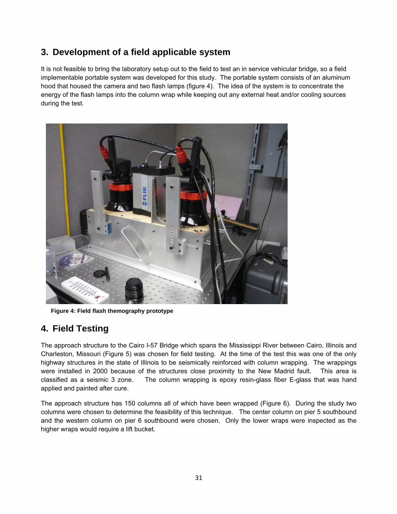
It is not feasible to bring the laboratory setup out to the field to test an in service vehicular bridge, so a field implementable portable system was developed for this study. The portable system consists of an aluminum hood that housed the camera and two flash lamps (figure 4). The idea of the system is to concentrate the energy of the flash lamps into the column wrap while keeping out any external heat and/or cooling sources during the test.

4. Field Testing

The approach structure to the Cairo I-57 Bridge which spans the Mississippi River between Cairo, Illinois and Charleston, Missouri (Figure 5) was chosen for field testing. At the time of the test this was one of the only highway structures in the state of Illinois to be seismically reinforced with column wrapping. The wrappings were installed in 2000 because of the structures close proximity to the New Madrid fault. This area is classified as a seismic 3 zone. The column wrapping is epoxy resin-glass fiber E-glass that was hand applied and painted after cure.

The approach structure has 150 columns all of which have been wrapped (Figure 6). During the study two columns were chosen to determine the feasibility of this technique. The center column on pier 5 southbound and the western column on pier 6 southbound were chosen. Only the lower wraps were inspected as the higher wraps would require a lift bucket.

Figure 4: Field flash themography prototype

32

Figure 5: Pulsed thermography column wrapping test system implemented in Cairo, IL.

Figure 6: Approach structure to the Cairo I-57 Bridge looking north on the Illinois side.

As a control, a tap test of the first wrapping (center column pier 5) was conducted and a disbond between the concrete and wrapping was located (Figure 7). This location was further investigated with thermography both passively (no flash lamps) and actively (with flash lamps). The active thermography method used in the study is Pulsed Thermography (PT). The test was conducted in February during morning with the air temperature

33

being 65 degrees Fahrenheit. The passive thermography detected the disbond as displayed in Figure 8. It was apparent that the footing was conducting ground temperature up the columns and subsequently the wrapping. The wrap that was separated from the column via disbond absorbed heat from the ambient air causing it to be warmer than the bonded wrap. The same section was then tested with the PT technique which vastly enhanced the image allowing for better quantitative data extraction from the image (Figure 8). The column was then further interrogated using the PT technique. The technique detected sub-surface defects in areas that appeared good on the surface. Since these defects were not detected using passive themography, it is believed that the technique is detecting a delamination between the wraps or a small disbond between the concrete and wrap. Each column has multiple wraps winding around the column, it was counted that the pier 5 columns were wrapped 10 times with a field measured thickness of around 3/8”.

The western most column on pier 6 was then interrogated using PT with similar results. The wrapping on this column consisted of 5 windings. A typical area indicating a subsurface defect was detected and displayed in figure 9 where a blade of grass is used as a pointer to indicate the location of the defect. Figure 10 displays the PT image of the area in figure 9, and indicates the presence of a subsurface defect in the area just below the pointer. The western exposure of this column to the sun posed a challenge during the inspection due to a heat gradient from one side to the other induced by the sun as displayed in figure 10. The lighter area on the left side is heating caused by the sun. As a result, it may be best to conduct this inspection in the shade if possible to eliminate this effect and/or conduct these inspections in the early morning hours.

Figure 7: Center column on pier 5 visual wrap/concrete disbond circled in yellow

34

Figure 8: Center column on pier 5 passive thermography image (left side) and PT image (right side). Horizontal field of view is 11 inches. Defect size is 1.63”x2.84”

Figure 9: Western column on pier 6 test area. Damage is located at the end of the pointer.

Figure 10: Western column on pier 6 PT image at 13.3 seconds. Defect size is 1.12”x1.11”

35

5. Conclusion

The passive themography technique worked well in detecting larger concrete/wrapping disbonds and possible delaminations between the wraps. With this technique it is possible to inspect a large area in minimal time. The passive thermography weakness lies in quantifying the disbond or delamination size and depth. The PT technique is slower but able to provide quantitative information related to the size and depth of the disbond or delamination. Once the wrap material properties are known a depth estimation is easily determined. The limits as far as the maximum thickness of wrapping that can be inspected using the PT technique still need to be determined. The flash hood needs a small modification to allow for a more evenly distributed flash that will eliminate “hot spots” on the top and bottom of the image. These spots can also be eliminated by decreasing the field of view of the camera. Additionally, post signal processing should be investigated to improve signal to noise ratio of the images. A single cart holding all the components of the system should also be implemented to ease the field inspection.

36

Chapter 5

Multiple Scattering of Lamb Waves by Multiple Corrosion Pits in a Plate Brandon W. Strom, Sridhar Krishnaswamy and Jan D. Achenbach

Abstract

The scattering of Lamb waves from multiple corrosion pits on the surface of a plate is investigated. Previous work produced a model which solved for the scattered field when a Lamb wave is incident on a single corrosion pit, and we present an improvement on that model, and use it to study the case of multiple corrosion pits. The solution technique solves for the scattered field by replacing the corrosion pits with equivalent point loads applied to the surface of the plate, and the reciprocity theorem is used to calculate the scattered field. For the case of multiple corrosion pits, an implicit set of equations are derived using the self consistent method, and an approximation is advanced which results in an explicit set of equations which approximate the scattered field. The second order approximation to the multiple scattering problem is considered and solved semi-analytically for an ensemble of corrosion pits.

1. Introduction

Structural health monitoring systems will revolutionize the maintenance schedules for fleets of aircrafts, resulting in increased safety and decreased costs. Such systems require measurement models in order to make sense of received waveforms influenced by the interaction of ultrasonic waves with damage. These waves carry information about damage which they have come into contact with, and the goal is to extract that information from the received waveforms. Our research in particular focuses on the interaction of Lamb waves with pitting corrosion on the surface of plate geometries which are commonly found in aerospace structures and commercial aircraft. Our model will allow us to analyze the effect of an incident Lamb wave scattering off of an ensemble of corrosion pits. Guided waves have been used extensively as an effective method to detect and characterize damage because of the scattering phenomena exhibited by them, as well as their ability to cover large areas due to low attenuation and loss of energy. As such, they are well suited as a diagnostic tool within the context of automated inspection, and are well understood; see the books by Achenbach1,2 for a thorough treatment of the subject. One of the most dangerous damage modes, which occur early on, is pitting corrosion. Pitting corrosion is a damage mode characterized by rapid penetration at discrete areas, has self-sustaining growth, and is one of the most dangerous forms of corrosion. In addition to the ability to penetrate through a plate, pitting corrosion causes a local stress concentration which assists in the onset of: brittle fracture, fatigue failure, stress corrosion cracking, and corrosion fatigue. Typically corrosion comes in the form of patches, so we will consider multiple scattering in order to better understand the interaction of Lamb waves with such a distribution of damage. Researchers have developed models for the single scattering of cavities in a plate for some time now. Grahn3 considered the scattering of an incident S0 mode from a cylindrical cavity in a plate. He then solved for the

37

A0, S0 and SH0 scattered fields using the wave function expansion technique. Finally, he used lower order plate theories to find simple approximations valid at lower frequencies. Cegla4 extended the work done by Grahn by using Mindlin plate theory instead of Kirchoff plate theory for the A0 mode, thereby extending the range of values which may be modeled for the frequency-thickness and wavenumber-damage radius products. Moreau5 generalized the geometry of this work and solved for the scattered field from a flat bottomed cavity where the radius of the cylindrical shaped cavity is a function of the angle. He provides an example for an elliptic shape and calculates the scattered A0, S0 and SH0 modes. Kim6 consider scattering by a notch in two dimensions based on work done by Cho7 which was done numerically using the Boundary Element Method. Many others have developed single scattering models as well, for example it is common to use the Finite Element Method, as done by Galan8. Recently the authors9 presented a model for the scattering of Lamb wave modes from a single spherical cavity in order to model the interaction of an incident Lamb wave with a corrosion pit in a plate. While many authors have studied the interaction of guided waves with single instances of damage, there have been much fewer that have studied them in the context of multiple instances of damage. When done, it is common to use a numerical approach and/or simple scatterer geometries in order to bypass the complexity of the multiple scattering problem. Martin10 uses a method similar to the one we adopt here, which dates back to Foldy11 in 1945. Martin calculates an effective wavenumber for the second order approximation of the scattered field. Deng12 considered the scattering of the S0 mode in a plate with multiple damage sites, and uses the single scattering model developed by Grahn and Cegla. This is done for a plate with cylindrical cavities. Sodagar13 studied obliquely incident plane acoustic waves scattering from an array of cylindrical shells immersed in a liquid. In the investigation they study resonance by considering higher order scattering. Lovstad14 modeled torsional waves scattering from multiple circular holes in a cylindrical geometry in an attempt to model the interaction of an incident wave with a corrosion patch in a pipe. To the best of the author’s knowledge, nobody has calculated an analytical solution to the multiple scattering of Lamb waves in a plate from spherical cavities representing damage caused by pitting corrosion. We begin by deriving a model for the multiple scattering of guided waves by use of the self-consistent method described in Martin15, which yields a set of equations that define the scattered field implicitly. Section three gives an overview of an algorithm to solve for the single scattering model, which we use to solve the multiple scattering problem. In section four we advance a set of approximations which result in a simplified explicit definition of the scattered field terms, and show that it may be used to obtain any order of accuracy if used iteratively. Finally we walk through a simple multiple scattering problem and show the reader how to explicitly construct the model for the second order contribution to the scattered field.

2. Derivation of Multiple Scattering Model

If we know about single scattering from a single obstacle in isolation, the best way to solve the problem of multiple scattering, according to Martin15, is by using a ‘self-consistent’ method. The total field is written as the sum of the incident field and scattered fields from each of the N individual corrosion pits. These scattered fields are unknown and we ultimately wish to solve for them. This relationship is written as

[ ]1

Ntot inc sc

nn

u u u

(1)

The effective field incident on the p-th corrosion pit, or radiation incident on the p-th corrosion pit in the presence of all other corrosion pits, then follows from eq. (2). It represents the effective field which is incident on the p-th corrosion pit due to all of the scattering effects, of all orders, from of all other corrosion pits.

[ ] [ ] [ ]1

Neff tot sc inc scp p n

nn p

u u u u u

(2)

38

We know that there exists a set of functions which relate the effective fields to the scattered fields, as represented by eq. (3). In the next section we will construct approximations to such functions, valid in the far field for small corrosion pits. It is important to recognize that we do not know the scattered or effective fields, but we do know how to construct approximations of the functions which relate them to each other. Each function maps an effective displacement field incident on the p-th pit to the scattered displacement field it in turn produces.

[ ] [ ] [ ] [ ]| , 1,2,...,sc effp p p pu u p N (3)

The power of this idea lies in the fact that we know how to construct approximations to these functions in closed form which map the effective fields incident on the corrosion pits to the corresponding scattered fields produced by them. It is uncommon to have explicitly constructed functions available for Lamb wave scattering problems due to their mathematical complexity. In the case of a single corrosion pit, the effective field incident on the corrosion pit is simply the incident field. We will derive a relationship, valid in the far field, for the scattered displacement field of the form given by eq. (3). If we substitute an effective field into this relationship as the incident field, the relationship still holds.

Now, using the definition given in eq. (2), we may rewrite eq. (3) as

[ ] [ ] [ ] [ ] [ ]1

1,2,...,N

sc eff inc scp p p p n

nn p

u u u u p N

(4)

This relationship is an exact equation defining the scattered fields. This is not trivial to solve, as these are actually functional relationships, and the scattered fields are defined implicitly, so it is much more complicated than simply inverting a matrix. We will now focus upon the functional relationship for the scattered field of a single corrosion pit due to an incident Lamb wave in a plate. The following section will give an overview of the algorithm used to construct the functional relationships, and the reader will be referred to the appendix and other papers for details of the derivation.

3. Single Scattering Model

For simplicity we will assume that the shape of the surface of the corrosion pit within the plate is perfectly spherical. Thus, the pit is defined by a cavity whose boundary is defined by a sphere centered above the plate. A diagram of the geometry for a spherical pit is given in fig. (1).

Figure 1: Model for corrosion pit in a layer

39

To simplify the problem we use superposition to split the total field (2a) into the sum of the incident (2b) and scattered (2c) fields. For the incident wave16 solution we calculate the tractions on the plate where the surface of the corrosion pit would be; we are assuming the plate is intact and the incident wave does not actually interact with a defect, that is, it is a virtual pit that is not actually there. For the scattered wave solution we take the equal and opposite of the previously found tractions across the surface defining the boundary of the corrosion pit. In summing these tractions we will have a traction free surface in (2a). We now focus upon the radiated field of (2c), which is the scattered field of (2a).

Figure 2a: Total field

Figure 2b: Incident field

Figure 2c: Scattered field

To further simplify the scattered field calculation we take the distribution of tractions in fig. (2c) and replace them by an equivalent point force which is obtained by integrating the traction field over the surface of the pit, and are applied on the surface of the plate. The point force is then decomposed in each spatial direction, and for each spatial direction we decompose the force into anti-symmetric and symmetric systems, as seen in fig. (3). As an example we show how a force due to an anti-symmetric incident wave is decomposed into anti-symmetric and symmetric systems, which are proportional to the anti-symmetric force caused by the anti-symmetric incident wave. The equations for the decompositions are given by eqs.(5,6). In the plane wave approximation with a spherical, hence symmetrically shaped cavity, there will only be force components in the direction of wave propagation and the direction perpendicular to the plate. It may be assumed that the approach proposed in this work is good for small pits in the far field, however it is not known at this time at what pit size the approximation will begin to diverge significantly from an exact solution of the scattering problem. Finally, we solve the resulting radiation problem by an application of the reciprocity theorem2.

Figure 3: Decomposition of an equivalent force representing the effect of a corrosion pit

40

( ) ( ) ( ) ( )2 2

A AA AS AAZ Z

Z Z Z

F FF z h z h z h z h F F (5)

( ) ( ) ( ) ( )2 2

A AA AS AAX X

X X X

F FF z h z h z h z h F F (6)

Recall the definition of an equivalent force over an area, which is obtained by integrating the traction field over the surface defining the area. The traction field is related to the stress field and normal to the surface and the stress field is related to the displacement field. We therefore see that the forces depend on the incident displacement field as well as the geometry of the surface; we will do this calculation in frequency space. We will be interested in calculating such integrals at arbitrary locations where the corrosion pits are located. This may be done in a very simply way by the following theorem for a traction free guided wave incident on a cavity.

Theorem

If iu is the displacement field of an incident guided wave such that the stresses ( ) 0iz z h are equal to

zero on the face of the plate surface and there is no body force, then the equivalent force for a small scatterer of volume V is given by

( ) ( )i i

V

F t u t dV or likewise in frequency space 2( ) ( )i i

V

F u dV (7)

Proof

Let the surface of the scatterer be defined as the union of the surface exposed to the plate face and the portion contained within the plate. The equivalent forces are given by

T I

i i i

S S

F t dS t dS (8)

The surface of the volume which bounds the corrosion pit within the plate may be written as T IV S S

where TS is the coin shaped surface on the top of the plate, and IS is the bowl shaped portion of the surface

within the plate. The first integral is zero since on the surface TS

ˆ ˆ( , , ) 0T T T

i ij j iz

S S S

t dS n dS x y z h zdxdy (9)

Equation (8) therefore reduces to

I

i i

S

F t dS (10)

If we apply the divergence theorem to the traction field over the volume confined by the cap T IV S S , we

find that we may instead write

,i ij j

V V

t dS dV

(11)

Now, since there are no body forces, the equations of motion are given by

,ij j iu or likewise in frequency space 2,ij j iu (12)

41

Therefore we may substitute and get

( ) ( )i i

V

F t u t dV or likewise in frequency space 2( ) ( )i i

V

F u dV (13)

QED

This is an advantage over our previous approach because we do not need to compute the various stress terms, but rather can simply plug in the relevant displacement term. Furthermore, we do not need to calculate the normal to a surface and calculate the differential surface terms, but rather we can simply integrate over a small volume defining the corrosion pit. In addition, this method lends itself well to a finite element package, and can now be used with more general shaped pits as long as we know the local displacement field in the absence of the pit, i.e. the base signal. As long as the corrosion pits are small, this approximation ought to hold well in the far field.

We will apply the reciprocity theorem to the equal and opposite of these forces, which are given by eq. (14) in frequency space. Notice that this can easily incorporate more general displacement fields where it would be extremely tedious to calculate the stress field using them. We must simply integrate them over a volume. Furthermore, the i-th component of the equivalent force depends only upon the i-th component of the incident displacement field, and the anti-symmetric force depends only upon the anti-symmetric portion of the incident field, and likewise for the symmetric portions. We use the notation here which indicates that , m A S is

either the anti-symmetric mode or symmetric mode.

2( )m mi i

V

F u dV (14)

In order to use the equivalent forces in the reciprocity theorem, we apply them to the top of the plate and thus have the body force per unit volume, applied at the point px

.

( ) ( )i i pf F x x (15)

It is important to again note that the incident A0 and S0 modes each individually give rise to a point force which is decomposed into a system that radiates both A0 and S0 scattered modes, thus helping to explain in a simple manner the mode conversion process. The diagram given in fig. (4) helps the reader to visualize this process. Using the equivalent forces, we apply the reciprocity theorem and solve17 for the scattered field amplitudes in the far field which allow us to then solve for the scattered Lamb wave modes. We have done this previously and refer the reader to our paper9 for a detailed analysis of the reciprocity theorem being used for this problem. The general form of the solution is given below in eq. (16). For the tensor relationship the first subscript defines the direction of the scattered displacement and the second subscript defines the direction of the applied force.

( )( )sc A S A S A Si ij j ij ij j j i iu C F C C F F u u (16)

Figure 4: Mode conversion between an incident wave and scattered waves

42

The scattered field is represented by a tensor relationship with two distinct terms: the equivalent forces which in the far field represents the presence of a corrosion pit, and the spatial dependence given by a compliance matrix. This representation is given below, and each term is decomposed into anti-symmetric and symmetric terms. We therefore see that each scattered mode has a contribution from each of the incident modes. The compliance matrix terms, found with the reciprocity theorem, are the spatial dependence terms which describe how the wave spreads out in space away from the point force which approximates the effect of the existence of the corrosion pit. The spatial variables are with respect to an origin being located at the point in which the equivalent forces are applied.

We now have a functional for each individual corrosion pit which maps the (effective) incident Lamb wave mode to the approximate scattered Lamb wave modes, which may be written by the general form given as eq. (17). We now revisit the multiple scattering model, and solve it by making a few simplifications and approximations in order to solve for the scattered field terms.

sc incu u

(17)

4. Approximations and Explicit Multiple Scattering Model

We now reconsider eq. (4) and advance an approximation to solve for the scattered fields which are thus far defined implicitly. An approach is as follows; we will do it for two corrosion pits for clarity. We begin with the first equation as given in eq. (18) and plug it into the second equation, as given by eq. (19).

[1] [1] [1] [2]sc inc scu u u

(18)

[2] [2] [2] [1] [2] [2] [1] [1] [2]sc inc sc inc inc scu u u u u u (19)

If we assume that the incident field is much larger than the scattered field of the second corrosion pit, given mathematically by eq. (20), we may approximate eq. (19) by eq. (21). This is a reasonable approximation because in general the incident field is significantly greater in magnitude than the scattered field it causes.

[2]inc scu u

(20)

[2] [2] [2] [1]sc inc incu u u (21)

If we now substitute eq. (21) into eq. (18) we get eq. (22).

[1] [1] [1] [2] [2] [1]sc inc inc incu u u u

(22)

If we again make a similar assumption that the incident field is much larger than the scattered field caused by it, given mathematically by eq. (23), we may approximate eq. (18) by eq. (24). Note that we must be in the far field of the pit for this approximation to hold. This again is a reasonable approximation based on the fact that the scattered field in general is significantly smaller in magnitude than the incident field which causes it.

[1]inc incu u (23)

[1] [1] [1] [2]sc inc incu u u (24)

43

We have now found an approximation, which we will refer to as a second order approximation, by using eqs. (21,24) instead of eqs. (18,19). If we solve eq. (4) generally for more pits, again making similar approximations, we find the approximation given by eq. (25). Note that we are assuming that there is a sparse collection of pits and we are interested in the far field solution.

[ ] [ ] [ ]1

[ ]N

sc inc incp p n

nn p

u u u higher order terms

(25)

Let us recall two equations now that we have, and show how we can get higher order approximations. We have the exact equation, given by eq. (4), and a second order approximation given by eq. (25). The approximation made here is related to the single scattering model. To see this, let us write these two equations again below.

[ ] [ ] [ ] [ ] [ ] [ ]1 1

N Nsc inc sc inc scp p n p p n

n nn p n p

u u u u u

(26)

[ ] [ ] [ ] [ ] [ ] [ ]1 1

[ ] [ ]N N

sc inc inc inc incp p n p p n

n nn p n p

u u u u u

(27)

This relation is uses the single scattering approximation, given in eq. (28). As a first order approximation we assume that the scattered field is primarily due to the incident field individually scattering off of each corrosion pit, and omit scattering due to the interaction of the individual scattered field with the corrosion pits. This approximation holds well when the spacing between the obstacles is large compared to the size of the obstacles and the wavelength of the incident wave.

[ ] [ ][ ]sc incp pu u (28)

In order to get higher order approximations, we may solve iteratively with known terms. The first order approximation is eq. (29). Plugging eq. (29) into the exact governing eq. (4) we get the second order approximation given by eq. (30). If we plug eq. (30) into eq. (4) we get a higher order approximation, given by eq. (31). This is very good because we are using known quantities to explicitly approximate eq. (4). Otherwise, it would be extremely difficult to solve eq. (4) for the scattered fields because they are defined implicitly.

[ ] [ ][ ]sc incp pu u

(29)

[ ] [ ] [ ]1

[ ]N

sc inc incp p n

nn p

u u u

(30)

[ ] [ ] [ ] [ ]1 1[ ]

[ ]N N

sc inc inc incp p n k

n kn p k n

u u u u

(31)

We thus have an iterative procedure to solve for the scattered field which in the limit will converges to the exact solution.

44

( 1)(0) ( )[ ] [ ] [ ] [ ]

1

0 ,N

incp p p n

nn p

u u u u

(32)

( )[ ] [ ]lim sc

p pu u

(33)

This makes physical sense because each additional term simply represents the effect of higher order pairwise scattering interactions, so we can choose the level of refinement in this way to any order of accuracy and in the limit it will converge to the true solution. We can choose the incident field, and once the pit locations/geometries are defined we know each of the functional relationships. Note we are using the wide spacing approximation15.

We will ignore the contribution of the SH0 scattered modes for now. The scattered SH0 mode has an insignificant contribution to the forward scattered field for small angles; the contribution is more significant at larger angles. For now we will be interested in modeling the interaction of Lamb waves with pits that are nearly in line with each other; future work will relax this assumption and include the SH0 modes. Moreover, by the time the scattered field of any given pit reaches another pit, the wavefront has a large enough radius of curvature to justify the plane wave approximation along the line connecting the center points of two pits. We therefore only have a resulting equivalent force with two components: one perpendicular to the face of the plane, and one parallel to the face of the plate in the direction connecting the two pits.

The result of this algorithm is that we have a cascading effect which may be solved via a recursion relation. An incident field interacting with a corrosion pit is replaced with an equivalent force which in turn causes a radiated field which is incident on another corrosion pit. This process is then repeated, and so we see that the point load representing a corrosion pit depends upon the point load of the previous pit which caused the incident wave. We will now work out a simple example to better illustrate this concept.

5. Application

Let us consider two corrosion pits, and show how we find the second order contributions to the scattered field. We will define a coordinate system with an origin located where an incident wave is launched from a transducer, and align our x-axis in the direction that the incident wave propagates. We will seek to detect the forward scattered field at a point directly across from the transducer generating the wave. We will locate our first corrosion pit on the x-axis a certain distance from the launching transducer, and the second corrosion pit will be located at an arbitrary location past the first corrosion pit. We will assume that the incident wave is a plane anti-symmetric A0 Lamb wave mode. We will solve for the individual second order scattering terms caused by the initial scattering off of the first corrosion pit which incident upon the second pit causes a set of second order radiated modes. We will solve for the z component of the displacements for each of these terms.

This problem is solved in a sequence of steps as follows; the reader is referred to figs. (5,6) to aid in the visualization of this process. The incident wave meets the first corrosion pit and scatters off of it. This is modeled by replacing the pit with equivalent forces, and finding the scattered A0 and S0 modes caused by the equivalent forces. Each of these radiated modes is then incident on the second corrosion pit, and the same process is repeated. At this point we assume that the wave is nearly planar once it reaches the second corrosion pit, and so the radial component of the force is defined as the in plane force with a new local coordinate system defined such that the x-axis is along the direction connecting corrosion pit one to corrosion pit two. Each cause scattered A0 and S0 Lamb wave modes, for a total of four second order terms emanating from the second corrosion pit. This same process also occurs by back scattering off of the second pit and then forward scattering off of the first pit, but for this paper we ignore these because we assume that the

45

second corrosion pit is located past the first and we are analyzing the forward scattered field; these terms would arrive later. We now walk through the mathematical details of these steps.

Figure 5: Geometry of the scattering problem for two corrosion pits viewed from above the plate

Figure 6: Diagram of the terms involved in the second order scattering process

We will assume that the incident wave is a plane A0 Lamb wave traveling in the positive x direction. The first corrosion pit is represented by an equivalent force which is decomposed into components in the x and z directions, and each of these are split into symmetric and anti-symmetric parts, which cause radiated A0 and S0 modes, respectively. The equivalent force due to the incident A0 wave is defined by eqs. (34,35). For these terms the subscript defines the directional component of the applied force, and the term in square brackets indicate that it is for the first corrosion pit.

1

2[1] 1 ,A inc

j j

V

F u dV j x z (34)

2 2 2 21 1 1 1 1 1 , , | ( ) ( ) ( ( )) , V x y z x x y y z h R D R z h (35)

The scattered field from the first corrosion pit, caused by the effect of the equivalent forces being applied to the surface of the plate, which will be incident on the second pit are given in eq. (36); the appendix defines these terms in detail.

sc A A S A A Si ij j ij j ij j i iu C F C F C F u u (36)

( , , )m mij ijC C r z (37)

The spatial variables are written with respect to a coordinate system with the origin located at the center of corrosion pit one, and x-axis is along the direction of propagation of the incident wave. We will need to calculate the radius and angle for corrosion pit two with respect to corrosion pit one, and these are given below.

2 212 1( )r x x y (38)

112 1tan ( / ( ))y x x (39)

46

The A0 and S0 modes radiated off of the first corrosion pit toward the second corrosion pit will each produce both A0 and S0 scattered modes due to their interaction with the second pit. The approach is the same for the A0 or S0 mode which is incident on the second pit due to scattering from the first pit. We again replace the corrosion pit by an equivalent force, except this time we make the plane wave approximation. We assume that the wave may be approximated as a plane wave once it arrives at the location of pit two. We then make a local coordinate system for corrosion pit two with an x-axis along the line connecting pit one to pit two, and let

x ru u so that x rF F ; see fig. (5) for the coordinate systems. Each is again split into anti-symmetric and

symmetric systems which radiate A0 and S0 modes. The equivalent force for pit two due to the , m A S

mode radiated by pit one is defined by eqs. (40,41).

2

2[2] 2 ,m m

j j

V

F u dV j x z (40)

2 2 2 22 2 2 2 2 2 , , | ( ) ( ) ( ( )) , V x y z x x y y z h R D R z h (41)

This is done for each of the incident A0 and S0 modes radiated from pit one, for a total of four terms which scatter off of the second corrosion pit. The scattered field terms are written as

( )( )sc A S A S AA SA AS SSi ij j ij ij j j i i i iu C F C C F F u u u u (42)

( , , )m mij ijC C r z (43)

The spatial variables are now written with respect to a coordinate system with the origin located at the center of corrosion pit two, and x-axis along the direction of a line which connects corrosion pit one to corrosion pit two. Therefore the spatial variable are written as

2 22 2 2( ) ( )mr x x y y (44)

1 12 2 2 2 2 1tan (( ) / ( )) tan ( / ( ))m y y x x y x x (45)

We now combine the results that we have just derived, and use them to construct the four terms below which describe the second order scattered field contribution of the second corrosion pit due to an incident anti-symmetric plane wave scattering off of the first corrosion pit, given by eqs. (46-49).

2 2 [2] 12 12 [1] 12 12 [1]

2 2 [2] 12 12 [1] 12 12 [1]

( , , ) [ ( , , ) [ ] ( , , ) [ ]]

( , , ) [ ( , , ) [ ] ( , , ) [ ]]

AA A A A A inc A A incz zx m m x xx x x xz z z

A A A A inc A A inczz m m z zx x x zz z z

u C r z F C r z F u C r z F u

C r z F C r z F u C r z F u

(46)

2 2 [2] 12 12 [1] 12 12 [1]

2 2 [2] 12 12 [1] 12 12 [1]

( , , ) [ ( , , ) [ ] ( , , ) [ ]]

( , , ) [ ( , , ) [ ] ( , , ) [ ]]

AS S A A A inc A A incz zx m m x xx x x xz z z

S A A A inc A A inczz m m z zx x x zz z z

u C r z F C r z F u C r z F u

C r z F C r z F u C r z F u

(47)

2 2 [2] 12 12 [1] 12 12 [1]

2 2 [2] 12 12 [1] 12 12 [1]

( , , ) [ ( , , ) [ ] ( , , ) [ ]]

( , , ) [ ( , , ) [ ] ( , , ) [ ]]

SA A S S A inc S A incz zx m m x xx x x xz z z

A S S A inc S A inczz m m z zx x x zz z z

u C r z F C r z F u C r z F u

C r z F C r z F u C r z F u

(48)

2 2 [2] 12 12 [1] 12 12 [1]

2 2 [2] 12 12 [1] 12 12 [1]

( , , ) [ ( , , ) [ ] ( , , ) [ ]]

( , , ) [ ( , , ) [ ] ( , , ) [ ]]

SS S S S A inc S A incz zx m m x xx x x xz z z

S S S A inc S A inczz m m z zx x x zz z z

u C r z F C r z F u C r z F u

C r z F C r z F u C r z F u

(49)

47

6. Results and Conclusion

For our simulation we fix the location of the transducer which launches the incident wave, the first corrosion pit the incident wave comes into contact with, and the sensor which detects the scattered field terms. The receiver is located 100 plate thicknesses from the launching transducer. The location of the second corrosion pit varies with respect to the first corrosion pit. It varies from 0 to π/4 radians with distances from 10h to 100h where the thickness of the plate is 2h. The incident wave has frequency 100Khz and the frequency-thickness product is fd = 0.635 Mhz mm. Our two pit sizes are the same, with sizes (R,D) = (1.00,0.25)/h. We have four scattered displacement fields which radiate off of the second corrosion pit, and we compare their magnitude at the receiver location to the first order contributions that scatter off of the first corrosion pit. The results are given in figs. (7,8).

We see that the second order contributions to the scattered field are small in magnitude compared to the first order terms, which indicate that higher order corrections to the scattered field are not necessary for the case we are considering, where the distribution of pits is sparse and individual cavities are small. This is acceptable because the goal is to detect corrosion early on, and this model would work for that case. Furthermore, we see that the ratio term uAA/uS is larger than the rest, and this is expected. The reason is that the incident wave is anti-symmetric, and the mode conversion from pit one is weak, while the forward scattered anti-symmetric wave from each pit remains dominant, thus the numerator is larger than the other terms, and the denominator is smaller than the forward scattered uA from pit one. We have thus shown how to construct the functional relationship derived in the previous sections, and argue that to second order it approximates the far field scattering well. Future work will aim to numerically validate this claim.

Figure 7: Ratio of second order scattered field displacements from pit two to the first order A0 mode radiated from pit one

48

Figure 8: Ratio of second order scattered field displacements from pit two to the first order S0 mode radiated from pit one

The next steps in this project will be to include the SH0 modes, and to investigate resonance for various ensembles of corrosion pits. The author is currently developing a more robust single scattering model which may be used with the approach described in this paper, thereby allowing for more densely spaced corrosion pits of larger sizes.

Appendix

According to the formulation of Achenbach2 the displacement field for a Lamb wave propagating in the positive x direction in Cartesian coordinates within an isotropic plate may be written as

, , ( ),0, ( ) ikx

x y zu u u u A iU z W z e (A1)

In cylindrical coordinates the wave which expands in the positive radial direction may be likewise written as

1 1, , ( ) ( , ), ( ) ( ) ( , ), ( ) ( , )r z ru u u u A k U z r kr U z r W z r (A2)

where, for a force applied in the z-direction causing a radially symmetric wave we have

(1)0( ) ( )r H kr (A3)

and for a force applied in the x-direction causing a wave with angular dependence we have

(1)1( , ) ( )cosr H kr (A4)

49

The depth dependent displacement terms, U(z) and W(z), may be written using eqs. (A5-A8).

2

2 2

2 sin( )( ) sin( ) sin( )

sin( )A A A

A AAA A

k q hU z p z q z

p hq k

(A5)

2 2 cos( )( ) cos( ) cos( )

2 cos( )A A A A A

A AA A A A

k q q h kW z p z q z

q k p h q

(A6)

2

2 2

2 cos( )( ) cos( ) cos( )

cos( )S S S

S SSS S

k q hU z p z q z

p hq k

(A7)

2 2 sin( )( ) sin( ) sin( )

2 sin( )S S S S S

S SS S S S

q k q h kW z p z q z

q k p h q

(A8)

The j component of equivalent force for the p-th pit due to an incident wave of mode m is written as

2[ ]

p

m mj p j p

V

F u dV (A9)

The compliance matrix, which describes the spatial dependence of the wave caused by the equivalent force being applied to a plate is a tensor relationship. The first subscript is related to the scattered displacement field component, and the second subscript is related to the equivalent force which depends on the incident field components. This is found by an application of the reciprocity theorem2 and details of the derivation are described in a paper written by the authors9.

'(1) '(1)1 0(1) (1)1 0

( ) ( ) ( ) cos ( ) ( ) ( )( , , ) ( )

4 ( ) ( ) ( ) cos ( ) ( ) ( )

m m m mm m mmij m m m m m

m m

H k r U z U h H k r U z W hkC r z

i I H k r W z U h H k r W z W h

(A10)

An application of the reciprocity theorem produces a term which is related to the orthogonality of the wave structure, and is defined as

( ( ) ( ) ( ) ( ))h

m m m m mxx xz

h

I T z U z T z W z dz

(A11)

The compliance matrix uses the Hankel functions defined by the sign convention given in eq. (A12)

(1) ( ) ( ) ( )m m mH k r J k r iY k r (A12)

The derivative terms are

'(1)1 1 2( ) ( ) / ( )m m m mH k r H k r k r H k r (A13)

and

'(1)0 1( ) ( )m mH k r H k r (A14)

50

References

[1] Achenbach, J. D., [Wave Propagation in Elastic Solids], North Holland, (1973). [2] Achenbach, J. D., [Reciprocity in Elasticity], Cambridge University Press, (2003). [3] Grahn, T., “Lamb wave scattering from a circular partly through-thickness hole in a plate,” Wave Motion 37, (2003). [4] Cegla, F.B., Rohde, A., Veidt, M., “Analytical prediction and experimental measurement for mode conversion and scattering of plate waves at non-symmetric circular blind holes in isotropic plates,” Wave Motion 45, (2008). [5] Moreau, L., Caleap, M., Velichko, A., Wilcox, P.D., “Scattering of guided waves by flat-bottomed cavities with irregular shapes,” Wave Motion 49, (2012). [6] Kim, B., Roh, Y., “Simple expressions of the reflection and transmission coefficients of fundamental Lamb waves by a rectangular notch,” Ultrasonics 51, (2011). [7] Cho, Y., Rose, J.L., “An elastodynamic hybrid boundary element study for elastic guided wave interactions with a surface breaking defect,” International Journal of Solids and Structures 37, (2000). [8] Galan, J.M., Abascal, R., “Elastodynamic guided wave scattering in infinite plates,” International Journal for Numerical Methods in Engineering 58, (2003). [9] Hao, S., Strom, B.W., Gordon, G., Krishnaswamy, S., Achenbach, J.D., “Scattering of the lowest Lamb wave modes by a corrosion pit,” Research in Nondestructive Evaluation 22, (2011). [10] Martin, P.A., Maurel, A., “Multiple scattering by random configurations of circular cylinders: Weak scattering without closure assumptions,” Wave Motion 45, (2008). [11] Foldy, L.L., “The multiple scattering of waves. I. General theory of isotropic scattering by randomly distributed scatterers,” Physical Review 67, (1945). [12] Deng, Q., Yang, Z., “Scattering of S0 Lamb mode in plate with multiple damage,” Applied Mathematical Modeling 35, (2011). [13] Sodagar, S., Honarvar, F., Sinclair, “Multiple scattering of an obliquely incident plane acoustic wave from a grating of immersed cylindrical shells,” Applied Acoustics 72, (2011). [14] Lovstad, A., Cawley, P., “The reflection of the fundamental torsional guided wave from multiple circular holes in pipes,” NDT&E International 44, (2011). [15] Martin, P.A., [Multiple Scattering, Interaction of Time-Harmonic Waves with N Obstacles], Cambridge University Press, (2006). [16] Achenbach, J. D., "Explicit solutions for carrier waves supporting surface waves and plate waves," Wave Motion 28, (1998). [17] Achenbach, J.D., Xu, Y., "Wave motion in an isotropic elastic layer generated by a time-harmonic point load of arbitrary direction," Journal of the Acoustical Society of America 106, (1999).

51

Chapter 6 Characterization of Water-Saturated Porous Cement Paste by a Laser Based Ultrasonic NDE Technique

Ningli Yang, Jae Hong Kim, Jeffrey J. Thomas, Oluwaseyi Balogun, and Sridhar Krishnaswamy

Abstract

A laser based ultrasonic technique is explored for predicting the mechanical integrity and durability of cementitious materials. It is well known that these properties depend on the mechanical properties, and structural properties including porosity and permeability. The technique used involves the measurement of the phase velocity of fast and slow longitudinal waves in water saturated cement paste. The slow wave velocity is related to the specimen’s tortuosity, which is closely related to the permeability. The fast wave speed is dependent on the elastic properties of porous solid. Experimental results detailing the generation and detection of fast and slow wave waves in freshly prepared and aged water-saturated cement samples with varying water-to-cement ratios are presented.

Introduction Cement paste is a critical binding material in concrete and its properties influence the structural integrity and durability of concrete structures. In the hydrated and hardened form, cement paste exhibits a multiscale fluid filled pore structure and an interconnected network of solid grains [1]. The properties of hydrated cement paste such as strength, durability, shrinkage, and fracture behavior are affected by its material and structural properties [2]. In particular, structural properties like porosity, tortuosity and permeability are widely recognized to influence the strength and durability of cement paste, and its resistance to penetrating aggressive agents can lead to material degradation [3]. Ultrasonic characterization techniques tailored to fluid-saturated materials continue to receive widespread attention in varying applications areas owing to their potential for nondestructive measurement of the structural and elastic properties of porous solids. In the context of cement paste, measurement of the velocity dispersion behavior and attenuation of ultrasonic waves have been commonly used for the characterization of the strength and durability of hydrated cement [4, 5].

Ultrasonic wave propagation in porous solids is commonly described using Biot’s phenomenological theory [6, 7]. The model considers the ultrasonic propagation through a porous material to comprise of the motion of the

52

solid skeleton and the pore fluid, which is coupled through elastic, inertia, and viscous forces. Unlike the general ultrasonic wave propagation in nonporous solids, Biot model leads to the generation of two bulk longitudinal waves namely the fast and slow waves, and a shear wave. The fast wave results from the motion of the solid skeleton and pore fluid in phase, while the slow wave results from the out-of-phase motion of the two phases. These waves exhibit marked dispersion and attenuation that are strongly sensitive to the elastic and structural properties of a porous solid. Of particular importance is the dispersion and attenuation of slow waves. The slow wave velocity approaches a constant asymptote at high frequencies that is related to the bulk wave velocity in the pore fluid and the tortuosity of the porous solid [8-10], while at low frequencies the slow wave attenuation is dominated by viscous forces that are related to the permeability and porosity [11]. As such, measurement of the slow wave dispersion provides a convenient approach for the characterization of the structural properties of porous materials. However, there is no experimental report on the ultrasonic generation and detection of slow waves in cement paste, which may be due to the strong attenuation effects that stem from viscous damping. This paper attempts to explore the generation and detection of fast and slow longitudinal waves in cement paste as a means to predict the mechanical integrity and durability of cementitious materials.

Cement paste has pores with different dimensions, and there is a frequency window where the attenuation coefficient is sufficiently low to observe a slow wave. Therefore the application of the traditional piezoelectric technique for studying wave propagation in porous materials is faced with certain difficulties due to low efficiency of piezoelectric excitation of wide-band ultrasonic pulses. Moreover, the transducer is not appropriate to test thick samples due to strong high-frequency ultrasonic attenuation in the materials. In this paper, ultrasonic characterization of water-saturated cement is investigated by a laser ultrasonic method. To produce powerful wide-band ultrasonic pulses, a pulsed laser source is used for ultrasonic wave generation and a narrowband fluid-immersion transducer is used for detection. Experimental results detailing the generation and detection of fast and slow wave waves in freshly prepared and aged water-saturated cement samples with varying water/cement ratios are presented. The sample tortuosity is determined from the slow longitudinal wave velocity, and the variation of the porosity of the specimens with the fast wave velocity is investigated. It is observed that the detection of the slow longitudinal wave depends on the sample age, which may be useful as a qualitative tool to assess structural changes in aging cementitious materials.

Background

Biot’s dynamic phenomenological models in fluid-saturated porous solids have been widely used to describe the characteristics of elastic wave propagation in porous materials. Using the assumption that there exists representative volumes in a porous material that is larger than the characteristic pore size and small compared to the acoustic wavelength, Biot described the dynamic mechanical motion of each representative volume in terms of the average displacement of the solid skeleton and the pore fluid. The result of Biot’s model is the prediction of two bulk longitudinal waves, namely the fast and slow waves, and a shear wave. The phase velocities of these waves are dispersive and are related to the structural and elastic properties of the porous material according to the following [9]:

2 2 2 1/ 2 2, 11 22 12 11 22 12 [ 4( )( )] / 2( )fw swV PR Q , (1a)

53

/[(1 ) (1 1/ ) ]sh s fV N , (1b)

where

22 11 122P R Q .

Vfw , Vsw, Vsh are the fast, slow, and shear wave velocities, and P, Q, R are generalized elastic coefficients which can be related to the bulk modulus of fluid Kf, the bulk modulus of solid Ks, the bulk modulus Kb of the skeletal frame, and the shear modulus N of both the skeletal frame and of the bulk material comprised of the skeletal frame and fluid. The density terms ρij are related to the density of the solid ρs and the fluid ρf by:

11 12 (1 ) s , (2a)

22 12 f , (2b)

The term ρ12 describes the inertial drag the fluid exerts on the solid:

12 (1 ) f . (2c)

where is porosity (fluid volume fraction), and α is the frequency dependent dynamic tortuosity [9] , which

accounts for the effects of viscous and inertia forces in the interaction between the pore fluid and the elastic frame. The fast and slow wave speeds are correspondingly frequency dependent. The application of Biot’s model requires a prior knowledge of the elastic coefficients, the porosity, and tortuosity. A simplification to the model results in the limit of the rigid skeleton approximation. Here, the solid skeleton is motionless and the phase velocity of the slow wave is non-dispersive at high frequencies following the simple relation:

/sw fV V . (3)

where Vf is the sound speed through the pore fluid and α is the high frequency limit of the dynamic tortuosity and it serves as a structure factor that accounts for the deviation of path of the connected pores from a straight wave propagation path. The tortuosity is equal to unity if the path of the connected pores is straight,

54

and greater than unity if the path is tortuous. The high frequency (f) limit beyond which Eqn. 3 is valid occurs where the viscous skin depth is smaller than the pore size,

2/f

f a (4)

where is the dynamic viscosity of the pore fluid and a is the characteristic pore size.

Measurement of the slow wave speed in this case provides a convenient approach to characterizing the tortuosity of a porous solid. Figure 1 shows a numerical calculation of the phase velocities of the slow, fast, and shear waves as a function of frequency in water saturated cement paste. The mechanical properties of cement paste are assumed to follow the values by Vlahinic et. al [12] for a water-to-cement ratio of 0.6. The tortuosity, permeability, and porosity of the cement paste was assumed to be 2.50, 2·10-17 m2 and 0.5 respectively. The slow wave velocity is lower than longitudinal wave velocity in water (1500 m/s). At low frequencies, the slow wave velocity exhibits strong positive dispersion, and approaches a horizontal asymptote at high frequencies. The fast wave and shear wave velocities also exhibit positive dispersion,

0 1 2 3 4 5 6 7 8500

1000

1500

2000

2500

3000

3500

4000

Frequency (MHz)

Ve

loci

ty(m

/s)

Shear waveSlow waveFast wave

FIGURE 1. Dispersion curves of bulk wave phase velocity for cement.

and are larger than the slow wave velocity. The fast and shear wave speeds are strongly dictated by the generalized elastic properties of the frame, while the slow wave speed depends on the bulk modulus of water (the pore fluid) and the porosity, permeability, and tortuosity of the cement paste.

55

Specimen Preparation

Two sets of porous cement samples were used. The first set consisted of three 8 month old cement specimens with water-to-cement ratios of 0.35, 0.50, 0.65. The second set consisted of freshly prepared water-saturated cement with a water-to-cement ratio of 0.60. Each of the specimens has a thickness of 6.00 mm. The porosity of each specimen was characterized using the standard Archimedes approach according to the following,

sat dry

w vol

M M

V

, (5)

where w is the volume density of water, volV is the volume of the specimen, dryM and satM are the masses

of the dried and water saturated sample. M dry for a given specimen was evaluated by drying the specimen in an oven for 12 hours at 70 degrees Celsius prior to weighing. The measured porosities are listed in Table 1.

Experimental Setup

Figure 2 shows a schematic diagram of the experimental setup used. Experiments are performed in a water tank filled with fresh water, and the tank incorporates a laser ultrasonic

TABLE 1. Porosity values of cement paste specimens with different water-to-cement ratios.

Sample 8 month Old Cement

Water/Cement Ratio 0.35 0.50 0.60

Porosity 27.0% 38.9% 46.4%

FIGURE 2. Experimental Setup.

56

system that is configured in the through-transmission mode. A pulsed laser (Pulse energy: 0.3 J, pulse duration: 8 ns, wavelength: 1064 nm) is used as the source to generate wide-band, short duration ultrasonic waves. A black tape attached to one side of a plastic wedge is used to enhance the laser generated ultrasound. The tape absorbs the pulsed laser energy, which leads to rapid heating, thermal expansion, and elastic wave generation. The generated elastic waves are coupled into the cement paste samples through the water, and a 3.5 MHz immersion transducer installed normal to the wedge and behind the specimen is used for ultrasonic wavedetection. The experimental configuration chosen favors the optimal coupling of longitudinal waves into the specimen. The measured time domain response of the transducer is digitized with an oscilloscope operated with a sampling rate of 1 GS/s.

Experimental Observation

First, the longitudinal wave velocities in a freshly prepared water-saturated cement paste with a water/cement ratio 0.60 were measured. Figure 3 shows the measured data obtained in the specimen. The waveforms show the direct fast longitudinal wave (FW) followed by a set of multiple reflections. The FW reflections are identified based on the round trip transit times between successive echoes. There is an additional arrival in the waveform that arrives at about 8.0 s, which does not correspond to a FW reflection. Since the experiment is performed at normal incidence where only longitudinal waves are expected, the ultrasonic mode is assumed to be the direct slow longitudinal wave (SW) arrival. The SW arrival is identified in the waveform, even when the specimen is scanned laterally with respect to the excitation and detection sources, thus ruling out of the possibly of the mode being a reflection from an internal defect. Furthermore, unlike the FW, no SW reflections are identified in the figure. This may be due to strong attenuation effects and low coupling of the longitudinal wave energy from the source into the slow wave. In addition, the pulse labeled FFSW in the figure arrives later than SW and it corresponds to a mode conversion of the FW to the SW or vice-versa. The measurement was repeated in the 8 month old cement paste specimens with porosity values listed in Table 1. The data obtained in each of the specimens is similar to that in Figure 3, with the exception that the SW and FFSW were not observed.

Results and Discussion

The tortuosity of the cement paste specimens is estimated from phase velocity of the slow wave using Eqn. 3, assuming that high frequency conditions apply here. The phase velocity of slow wave was obtained from the measured data using the substitution technique in through-transmission mode [13]. In the substitution method, the longitudinal wave transmitted directly from the source to the receiver without the specimen is used as a reference signal. The time difference between the arrival times of the SW in Figure 3 and the reference signal is obtained by cross-correlation and used to determine the SW phase velocity Vsw using the following expression:

.

( . )w

sww

V hV

h V t

(6)

57

0 4 8 12 16

-0.012

-0.008

-0.004

0.000

0.004

0.008

0.012

Am

plitu

de (

mV

)

Time (s)

3.5M

Figure 3. Bulk longitudinal waves in a cement paste specimen.

where Vw is longitudinal wave velocity in water, t is the time difference, and h is the specimen thickness.

Note that for this experiment, the distance between the excitation source and the ultrasonic transducer was held constant. The phase velocity of slow wave in the freshly prepared cement paste specimen is estimated using Eqn. 6 to be 925 m/s, which is close to the theoretical value shown in Fig. 1 at high frequencies. Using the SW velocity in Eqn. 3, the specimen tortuosity is estimated to be 2.63, which indicates that the propagation of path of the SW through the connected pores is not straight. Measurement of the SW phase velocity as a function of frequency is needed to reliably predict the high frequency limit, and to accurately estimate the tortuosity.

The tortuosity of the 8 month old cement paste specimens could not be estimated because the SW was not observed in the specimens. The absence of the SW is assumed to be due to a change in the pore connectivity with age since the slow wave speed primarily results from wave propagation through the pore fluid [14]. The SW measurement approach used here may provide a suitable approach to characterizing the permeability of cement paste, owing to the direct correlation between tortuosity and permeability [15].

Phase Velocity‐Porosity Relationship

Cement durability is also related to porosity, which determines the intensity of interactions of the material with aggressive agents. The influence of porosity on the fast wave velocity was investigated in the 8 month old specimens in order to investigate the effect of porosity on ultrasonic parameters. The phase velocity Vfw of the

fast wave was obtained using the auto-correlated time difference 1t between successive amplitude peaks of

the fast wave echoes in the measured data in the following expression:

12 /fwV h t . (7)

3F 5F

FW SW FFS

58

Table 2. Phase velocity of the fast wave in water and air saturated cement paste specimens.

Porosity (%)

Fast Wave Phase Velocities (m/s)

Water Saturated Dried Re‐saturated

Over Night One Week

27.0 4326 3938 3948 3982

38.9 3862 3440 3484 3534

46.4 3483 3070 3078 3141

It is implicitly assumed in Eqn. 7 the fast wave velocity is constant with frequency. The fast wave phase velocity was measured in water saturated, dried (or air saturated), and re-saturated specimens respectively. The experimental setup was slightly modified to perform the experiments in the dried specimen. A black tape was placed on one side of the specimen and illuminated with the excitation laser for the generation of ultrasound. The detection transducer was positioned on the other side of the specimen and on epicenter with the generation source. A thin film of ultrasonic coupling fluid was placed between the specimen and the transducer totransmission of ultrasound from the specimen. The specimens were re-saturated in water and tested in the experimental setup shown in Figure 2 The measured fast wave phase velocities obtained in the specimens are shown in Table 2. The velocity decreases with porosity in the specimens, which results from the corresponding decrease in the frame elastic properties. For a fixed porosity, the fast wave velocity is seen to be smaller in the dried sample compared to the water saturated case, and the velocity increases with time in the re-saturated specimens. The measurements were made in the re-saturated specimens after soaking in water overnight (~12 hours) and after one week.

This trend indicates that the elastic properties of the frame decreases upon drying and increases with time as the specimens are re-saturated. The lower value of the fast wave velocity in dried specimen may result from the reduction in the effective properties of the porous solid due to the smaller value of the bulk modulus of pore fluid in the air saturated (dried) specimen compared to the water saturated specimen. However, the gradual increase in the velocity with time in the re-saturated specimens can be attributed to re-saturation effects with hydration. The latter effect is well known in cement paste [14]. Furthermore the pore structure in cement paste is known to change with drying and hydrating [16], which is another explanation of the velocity variation.

Conclusion

The ultimate goal of this work is to develop an ultrasonic technique that allows for the monitoring of changes in structural properties like permeability of cementitious materials as the material ages. The permeability depends on the porosity and tortuosity, and measurement of these properties can provide a means to

59

monitoring the durability of cement based materials. As a first step, a laser based ultrasonic NDE technique is explored for the generation and detection of fast and slow longitudinal waves in hydrated cement paste. The slow wave speed depends on the tortuosity and permeability, while the fast wave speed strongly controlled by the elastic properties of the porous solid. The slow wave speed was measured in a freshly prepared cement paste specimen with a water-to-cement ratio of 0.6, from which the tortuosity of the specimen was determined. However, the slow wave was not observed in the 8 month old hydrated specimens with a range of water-to-cement ratios. The absence of the slow wave is assumed to be due to a change in the pore connectivity with age since the slow wave speed results from wave propagation through the pore fluid. In addition, the phase velocity of the fast wave was measured in the 8 month old specimens for varying porosities, pore fluids, and re-saturation times. The velocity changes obtained was interpreted as the influence of changes in the elastic properties and pore structure of the specimens with processing (drying and re-saturation). The preliminary results obtained shows that this approach may be a viable approach to monitoring the durability of cementitious materials. The accuracy and reliability of the measurement technique is yet to be established.

References

1. C. M. Sayers and A. Dahlin, Advanced Cement Based Materials 1, 12‐21 (1993).

2. P. Mondal, S. P. Shah, and L. Marks, Cement and Concrete Research 37, 1440‐1444 (2007).

3. D. Breysse and B. Gerard, Cement and Concrete Research 27, 761‐775 (1997).

4. J. S. Popovics, W. Song, J. D. Achenbach, J. H. Lee, and R. F. Andre, Journal of Engineering

Mechanics‐Asce 124, 1346‐1353 (1998).

5. Z. Lafhaj, M. Goueygou, A. Djerbi, and M. Kaczmarek, Cement and Concrete Research 36,

625‐633 (2006).

6. M. A. Biot, Journal Of The Acoustical Society of America 28, 168‐178 (1956).

7. M. A. Biot, Journal Of The Acoustical Society of America 28, 179‐191 (1956).

8. D. L. Johnson, Applied Physics Letters 37, 1065‐1067 (1980).

9. D. L. Johnson and T. J. Plona, Journal of the Acoustical Society of America 72, 556‐565

(1982).

10. J. F. Allard, B. Castagnede, M. Henry, and W. Lauriks, Review of Scientific Instruments 65,

754‐755 (1994).

11. D. L. Johnson, J. Koplik, and R. Dashen, Journal of Fluid Mechanics 176, 379‐402 (1987).

12. I. Vlahinic, H. M. Jennings, and J. J. Thomas, Mechanics of Materials 41, 319‐328 (2009).

60

13. P. H. F. Nicholson, G. Lowet, C. M. Langton, J. Dequeker, and G. VanderPerre, Physics in

Medicine and Biology 41, 2421‐2435 (1996).

14. P. Navi and C. Pignat, Cement and Concrete Research 29, 507‐514 (1999).

15. P. Xu and B. M. Yu, Advances in Water Resources 31, 74‐81 (2008).

16. I. O. Yaman, N. Hearn, and H. M. Aktan, Materials and Structures 35, 102‐109 (2002).

61

Chapter 7 Room-temperature Humidity Sensing Using Graphene Oxide Thin Films Gautam Naik, and Sridhar Krishnaswamy

Abstract In this article, we report on a room-temperature humidity sensing device using graphene oxide (GO) thin films synthesized by chemical exfoliation. Changes in the device conductivity are measured for varying relative humidity in the experimental chamber. Experiments are carried out for relative humidity varying from 30% to 75%. We observe a difference in the results obtained for low relative humidity (<50%) and high relative humidity (>50%), and propose a sensing mechanism to explain this difference. The sensing device has high sensitivity and fast response time.

1. Introduction Humidity sensors are in large demand in industry, environmental, and structural monitoring fields. One of the most frequent causes of structural failure is corrosion. A large number of structures degrade and fail due to inefficient humidity monitoring. A lot of research has been conducted to fabricate high efficiency humidity sensors, based on either change in resistance [1–3] or mass [4, 5], of a thin film due to the presence of water molecules. More recently, humidity sensors for corrosion detection were fabricated using long period gratings by calculating the resonant wavelength shift [6]. In recent years, research has been conducted to achieve a high level of sensitivity and selectivity in sensors. Here especially, carbon-based materials like graphene have raised great interest for various types of applications, due to their excellent electronic properties, high levels of thermal conductivity, stiffness and strength, and excellent adsorption properties. Graphene was first isolated in 2004 [7], and is best described as a two-dimensional single-atom thick sheet of sp2 hybridized carbon atoms arranged in a honeycomb lattice, and is the basic building block for all graphitic materials [8]. Schedin et al. were one of the first to demonstrate the potential of using graphene for detection of gases [9]. Since then, research has been conducted to demonstrate the use of graphene, and its derivative graphene oxide, to fabricate nanoscale sensors to detect various gases such as CO2, NO2, NH3. Lu et al. demonstrated using thermally-reduced graphene oxide to fabricate high-performance sensors to detect NO2 and NH3 in air [10, 11]. Lange et al. used a graphene-palladium nanoparticle composite to detect hydrogen in air [12]. Nomani et al. achieved high sensitivity and selectivity with sensors fabricated using epitaxial graphene [13]. Jeong et al. fabricated a flexible NO2 sensor based on hybrid films based on carbon nanotubes and graphene [14]. Yoon et al. reported a CO2 gas sensor using graphene fabricated by mechanical cleavage [15]. Robinson et al. demonstrated the use of reduced graphene oxide to detect chemical-warfare agents and explosives at parts-per-billion concentrations [16].

62

A limited amount of work has been done with regards to humidity detection using graphene and graphene oxide. Massera et al. reported using a graphene sheet as a humidity sensor [17]. Yao et al. demonstrated the sensitivity of graphene oxide to humidity by using it as a coating on quartz crystal microbalances [18]. However, most of the work done for gas and humidity sensing has been done at the micro-and nanoscale. Taking advantage of the excellent sensitivity and selectivity of nanomaterials such as graphene to fabricate large-area sensors is crucial. In this work, we examine the humidity sensing characteristics of large-area graphene oxide thin films. For this purpose, we fabricate humidity sensing devices using graphene oxde synthesized using chemical exfoliation and conduct experiments at various humidity levels. Possible humidity sensing mechanisms of the sensors are also discussed.

2. Material and Methods 2.1. Materials and Equipment To prepare graphene oxide, graphite, sulphuric acid (H2SO4, 98%), sodium nitrate (NaNO3), potassium permanganate (KMnO4), and hydrogen peroxide (H2O2, 30 wt.% ) were obtained from Alfa Aesar. Graphite, NaNO3, and KMnO4 were used as obtained. To dilute H2SO4 and H2O2 to required concentrations, Milli-Q deionized water with resistivity of ∼18 MΩ-cm was used. Experiments were carried out in a sealed plastic chamber. To measure conductivity, a Keithley 2400 source meter was used. Humidity was introduced in to the chamber using a commercial mini-humidifier. Relative humidities and temperatures inside the chamber were monitored using a model TH804 commercial humidity monitor manufactured by Nicetu. 2.2. Sample Preparation Graphene oxide (GO) was prepared using the Hummers’ method [19]. GO paper samples were prepared using bottle-top vacuum filtration of GO in water through a 47 mm diameter Whatman filter with a pore size of 0.02 µm. The GO papers were left overnight to dry at room temperature. The humidity sensors were fabricated by cutting out 10 mm wide, 30 mm long rectangular samples from the GO papers obtained by filtration. From scanning electron microscope images, as shown in Fig. 1(a), the thickness of the samples is obtained to be ∼26 µm. Copper wires (diameter 0.005 in) were bonded as electrodes to the GO samples using CircuitWorks conductive epoxy, and left to dry overnight. Figure 1(b) shows some of the humidity sensing devices fabricated. 2.3. Characterization The fabricated GO paper was imaged using a Hitachi scanning electron microscope equipped with secondary electron detectors. Imaging was done at 20 kV acceleration voltage and 10 µA emission current. To characterize the atomic weight percentage of different elements present in the GO paper, energy-dispersive x-ray spectroscopy was carried out in the scanning electron microscope. Raman spectra were obtained using a Acton TriVista CRS Confocal Raman System, with a laser wavelength of 514.5 nm. Powder x-ray diffraction spectra were obtained using a Rigaku DMAX diffractometer. 2.4. Humidity Sensing Experiments To characterize the performance of the fabricated graphene device as a humidity sensor, we measured the change in its resistance upon exposure to varying relative humidities inside the chamber. As illustrated in Fig. 2, the graphene device is enclosed in a chamber with the commercial humidifier and humidity monitor. The copper electrodes are connected to the Keithley 2400 source meter using alligator clips, which might introduce some contact resistance. A controlled test with a known resistance of 98 Ω showed less than 0.1% variability on exposure to humidity. Thus, a change in contact resistance due to humidity is ruled out. The source meter is connected to a PC using a GPIB interface, where the data is acquired using LabVIEW. Figure 3 shows the complete experimental setup. All experiments are carried out at room temperature (24 ±1 C).

63

3. Results and Discussion

3.1. Characterization Figure 4 shows the powder x-ray diffraction spectra of graphene oxide and graphite. Peak 2θ angles of 9.14 and 26.7 are obtained for graphene oxide and pristine graphite, which correspond to an interlayer spacing of 0.96 and 0.34 nm respectively. Figure 5 shows the Raman spectrum of graphene oxide. D and G peaks are clearly seen in the spectrum, with a slight red shift of the G peak towards 1600 cm−1. Elemental characterization of graphene oxide was carried out using energy-dispersive x-ray spectroscopy. Table 1 shows the atomic percentage of elements present in the fabricated GO device.

(a) SEM Image of Device Cross-section

(b) Humidity sensing devices

Figure 1: SEM image of cross-section and fabricated sensing devices

Figure 2: Humidity chamber

64

Figure 3: Experimental setup

Figure 4: X-ray Diffraction spectra of graphene oxide and graphite

Element Atomic%

Carbon 65.93 Oxygen 33.34

Others (P, S, K, etc.) 0.73

Table 1: Element analysis for graphene oxide

65

3.2. Humidity Sensing Experiments To characterize the performance of the sensing device, humidity is infused into the chamber using the mini-humidifier. Figure 6(a) shows the time response of the GO humidity sensing device, when the humidity was increased from 30% to 60%. At 90 s into the data recording, the humidifier is switched ON for 30 s. Infusion of humidity into the chamber decreases the resistance drastically. Figure 6(a) shows the relative resistance of GO after humidity infusion (R) compared to the resistance in ambient air (R0). Resistance data is normalized to exclude the variability in resistance between devices and also the slight contact resistance that might be caused due to the use of alligator clips. An extremely large decrease in resistance (∼98%) is observed. This shows that a large amount of water vapor is adsorbed on the surface of GO, which increases its conductivity drastically. The resistance of GO reaches within 5% of its steady-state value within 140 s, whereas the commercial humidifier takes 1200 s to display a steady reading. This shows that the sensing device has a very fast response. To study the performance of the sensor for decreasing humidities, the chamber was opened while at 60% RH. The humidity in the chamber decreased with time, and equilibrated with the room conditions of 30% RH. Figure 6(b) shows the time response of the sensor as the humidity decreases from 60% to 30% RH. The decrease in humidity inside the chamber causes an immediate increase in resistance. The resistance is normalized to the resistance R0 of the GO device before starting the entire experiment, i.e. before the humidity is increased from 30% to 60%. It is observed that the resistance of the GO device after one cycle from 30% to 60% RH and back is higher than its original resistance R0. This indicates that there is some vapor content that gets absorbed into the GO device, thereby increasing its resistance. This makes it important to study the humidity hysteresis characteristics of these sensors. Humidity hysteresis characteristic is an important parameter to characterize the performance of humidity sensors. To examine this characteristic in the GO device, two sets of cyclic experiments were carried out. In the first case, the humidity was cycled between 30% and 50%, and between 30% and 75% in the second case. Figures 7 and 8 show the time response of the device for these cases, respectively. In each case, the following procedure was followed: 1. the humidifier was switched ON to increase the humidity in the chamber to the required level, 2. the resistance was recorded for increasing humidity for 1200 s, 3. the chamber opened to decrease the humidity to room conditions, 4. the resistance recorded for decreasing humidity for 1200 s. This procedure is repeated for the required number of cycles. Figure 7 shows the time response of the device for humidity ranging from 30% to 50%. The sensing device shows high sensitivity, even for a 20%

Figure 5: Raman spectrum of graphene oxide

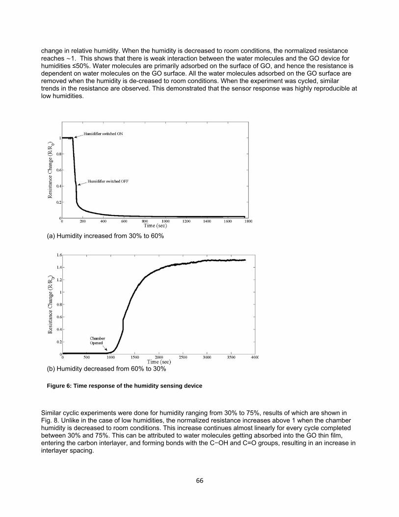
66

change in relative humidity. When the humidity is decreased to room conditions, the normalized resistance reaches ∼1. This shows that there is weak interaction between the water molecules and the GO device for humidities ≤50%. Water molecules are primarily adsorbed on the surface of GO, and hence the resistance is dependent on water molecules on the GO surface. All the water molecules adsorbed on the GO surface are removed when the humidity is de-creased to room conditions. When the experiment was cycled, similar trends in the resistance are observed. This demonstrated that the sensor response was highly reproducible at low humidities. Similar cyclic experiments were done for humidity ranging from 30% to 75%, results of which are shown in Fig. 8. Unlike in the case of low humidities, the normalized resistance increases above 1 when the chamber humidity is decreased to room conditions. This increase continues almost linearly for every cycle completed between 30% and 75%. This can be attributed to water molecules getting absorbed into the GO thin film, entering the carbon interlayer, and forming bonds with the C−OH and C=O groups, resulting in an increase in interlayer spacing.

(a) Humidity increased from 30% to 60%

(b) Humidity decreased from 60% to 30%

Figure 6: Time response of the humidity sensing device

67

Figure 9 illustrates the proposed sensing mechanism of GO. We propose that the change in resistance due to humidity is caused by the adsorption of water molecules on the surface of GO, as well as the absorption of water molecules into the GO thin film. The adsorption of water molecules on the surface causes a decrease in resistance, whereas absorption causes an increase in resistance due to an increased interlayer spacing. Although these two mechanisms take place simultaneously, at low humidity, the adsorption mechanism results in a much larger decrease in resistance than the increase in resistance due to absorption of water molecules. At higher humidity, since more water molecules get absorbed into the GO thin film, there is a larger increase in resistance, which is clearly observed in the response curves shown previously. To confirm the increase in interlayer spacing after exposure to high humidity, x-ray diffraction spectra were obtained for the GO device exposed to 75% RH. Figure 10 shows a comparison of the x-ray diffraction spectra of GO before and after exposure. The interlayer spacing is increased from 0.96 nm to 1.27 nm. This increase in interlayer spacing, we propose, is due to the bonding between the dissociated H2O molecules (H2O=H++OH−) and the C−OH and C=O groups.

Figure 11 shows a summary of all the experiments performed in this work. The experimental data is fitted with a power equation of the form AxB + C. The humidity sensing device shows sensitivity at all ranges, while being highly sensitive for large changes in humidity.

Figure 8: Time response of the humidity sensing device, for humidity ranging from 30% to 75%

68

Figure 9: Illustration of the humidity sensing mechanism

Figure 10: Comparison of XRD spectra before and after exposure to 75% RH

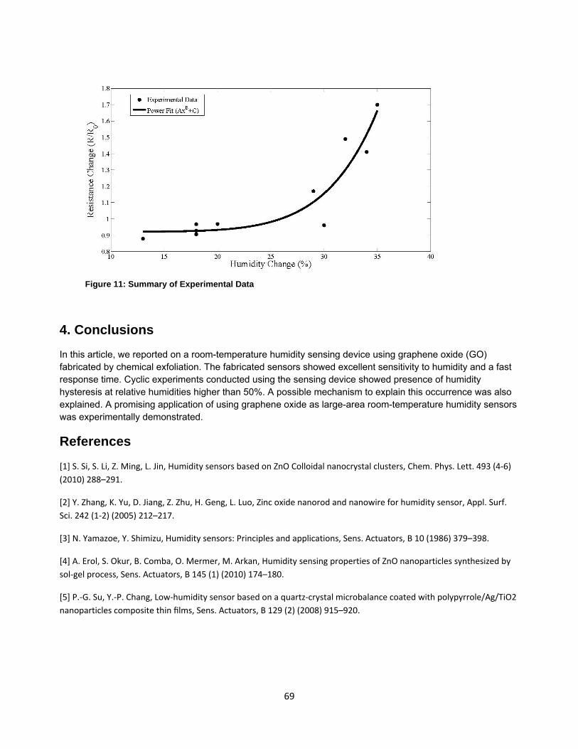
69

4. Conclusions

In this article, we reported on a room-temperature humidity sensing device using graphene oxide (GO) fabricated by chemical exfoliation. The fabricated sensors showed excellent sensitivity to humidity and a fast response time. Cyclic experiments conducted using the sensing device showed presence of humidity hysteresis at relative humidities higher than 50%. A possible mechanism to explain this occurrence was also explained. A promising application of using graphene oxide as large-area room-temperature humidity sensors was experimentally demonstrated.

References

[1] S. Si, S. Li, Z. Ming, L. Jin, Humidity sensors based on ZnO Colloidal nanocrystal clusters, Chem. Phys. Lett. 493 (4‐6)

(2010) 288–291.

[2] Y. Zhang, K. Yu, D. Jiang, Z. Zhu, H. Geng, L. Luo, Zinc oxide nanorod and nanowire for humidity sensor, Appl. Surf.

Sci. 242 (1‐2) (2005) 212–217.

[3] N. Yamazoe, Y. Shimizu, Humidity sensors: Principles and applications, Sens. Actuators, B 10 (1986) 379–398.

[4] A. Erol, S. Okur, B. Comba, O. Mermer, M. Arkan, Humidity sensing properties of ZnO nanoparticles synthesized by

sol‐gel process, Sens. Actuators, B 145 (1) (2010) 174–180.

[5] P.‐G. Su, Y.‐P. Chang, Low‐humidity sensor based on a quartz‐crystal microbalance coated with polypyrrole/Ag/TiO2

nanoparticles composite thin films, Sens. Actuators, B 129 (2) (2008) 915–920.

Figure 11: Summary of Experimental Data

70

[6] S. Zheng, Y. Zhu, S. Krishnaswamy, Nanofilm‐coated long‐period fiber grating humidity sensors for corrosion

detection in structural health monitoring, in: Proc. SPIE, Vol. 7983, San Diego, California, USA, 2011, pp. 79831A–

79831A–9.

[7] K. S. Novoselov, A. K. Geim, S. V. Morozov, D. Jiang, Y. Zhang, S. V. Dubonos, I. V. Grigorieva, A. A. Firsov, Electric

field effect in atomically thin carbon films, Science (New York, N.Y.) 306 (5696) (2004) 666–9.

[8] A. Geim, K. Novoselov, The rise of graphene, Nat. Mater. 6 (3) (2007) 183–91.

[9] F. Schedin, A. K. Geim, S. V. Morozov, E. W. Hill, P. Blake, M. I. Katsnelson, K. S. Novoselov, Detection of individual

gas molecules adsorbed on graphene., Nat. Mater. 6 (9) (2007) 652–5.

[10] G. Lu, L. E. Ocola, J. Chen, Reduced graphene oxide for room‐temperature gas sensors, Nanotechnology 20 (44)

(2009) 445502.

[11] G. Lu, L. E. Ocola, J. Chen, Gas detection using low‐temperature reduced graphene oxide sheets, Appl. Phys. Lett.

94 (8) (2009) 083111.

[12] U. Lange, T. Hirsch, V. M. Mirsky, O. S. Wolfbeis, Hydrogen sensor based on a graphene‐palladium

nanocomposite, Electrochim Acta 56 (10) (2011) 3707–3712.

[13] M. Nomani, R. Shishir, M. Qazi, D. Diwan, V. Shields, M. Spencer, G. S. Tompa, N. M. Sbrockey, G. Koley, Highly

sensitive and selective detection of NO2 using epitaxial graphene on 6H‐SiC, Sens. Actuators, B 150 (1) (2010) 301–307.

[14] H. Y. Jeong, D.‐S. Lee, H. K. Choi, D. H. Lee, J.‐E. Kim, J. Y. Lee, W. J. Lee, S. O. Kim, S.‐Y. Choi, Flexible room‐

temperature NO2 gas sensors based on carbon nanotubes/reduced graphene hybrid films, Appl. Phys. Lett. 96 (21)

(2010) 213105.

[15] H. J. Yoon, D. H. Jun, J. H. Yang, Z. Zhou, S. S. Yang, M. M.‐C. Cheng, Carbon dioxide gas sensor using a graphene

sheet, Sens. Actuators, B 157 (1) (2011) 310–313.

[16] J. T. Robinson, F. K. Perkins, E. S. Snow, Z. Wei, P. E. Sheehan, Reduced graphene oxide molecular sensors, Nano

Lett. 8 (10) (2008) 3137–40.

[17] E. Massera, V. L. A. Ferrara, M. Miglietta, T. Polichetti, I. Nasti, G. D. I. Francia, Gas sensors based on graphene,

Chemistry Today 29 (2011) 39–41.

[18] Y. Yao, X. Chen, H. Guo, Z. Wu, Graphene oxide thin film coated quartz crystal microbalance for humidity

detection, Appl. Surf. Sci. 257 (17) (2011) 7778–7782.

[19] W. Hummers, R. Offeman, Preparation of graphitic oxide, J. Am. Chem. Soc. 80 (6) (1958) 1339–1339.

71

Chapter 8

Probabilistic Considerations Are Essential to QNDE and SHM

Jan D. Achenbach, Moshe L. Cohen, and Salil S. Kulkarni

ABSTRACT

Probabilistic considerations play a dominant role in the four stages of the diagnostics and prognostics of fatigue damage in metals. Considerable attention has been given to the evolution and detection of pre-crack fatigue damage and the probabilistic aspects of subsequent macrocrack formation (Stage 1). For Stage 2 (macrocrack growth and detection), Paris law for crack growth under cyclic loading conditions can be useful, particularly if it is placed in a probabilistic context, and if the constants in the law are represented by probability distributions. By introducing the probability of detection concept, various probabilities related to the existence, after N cycles, of a crack larger than a critical size, can be determined in Stage 3 for purposes of prognostication. Paris law has its limitations and efforts to formulate other crack-growth laws will be mentioned. Finally, we will mention probabilistic aspects of optimizing the inspection schedule for Stage 4.

INTRODUCTION A Structural Health Monitoring (SHM) system based on permanently installed sensors at critical locations uses the techniques of non-destructive testing (NDT) to provide continuous (or on-demand) information about the state of a structure, so that an assessment of the structural integrity can be made at any time, and timely remedial actions may be taken as necessary. A large number of sensors forms the front end of an SHM system to gather information on the condition of the structure. The information from the sensors is incorporated into structural analyses and failure models to assess the state of the structure and to estimate the remaining lifetime. Thus, the underlying concept is based on detecting and characterizing damage and assessing it in terms of failure mechanics and damage growth laws. A probabilistic approach is essential in both the diagnostic and prognostic components of SHM.

There are many technical challenges to be overcome with regard to sensor development and data transmission. Some sensors should be designed to measure a well-specified signal, whereas others should be able to measure a broad diversity of signals. This is important for both the diagnostics and prognostics aspects of SHM. To satisfy this objective, measurement models play a significant role. A measurement model’s principal purpose is to predict from first principles the sensor’s response to specific anomalies in a given structure, and inversely to provide design guidelines for sensor development.

An important component of sensor development is the probability of detection (POD) concept. This is a representation of the probability that a given measurement system will be able to detect specific damage in a

72

given material/structure. It incorporates knowledge of the signal detected by the measurement system together with statistical information concerning flaw distributions and instrumental noise/thresholding levels. A POD curve shows the probability of a flaw’s detection as a function of flaw size for a specific inspection technique.

Until recently, essentially all applications of the POD concept have been empirical, i.e., a statistically significant number of samples are prepared with artificial flaws and then experiments are made by a number of operators to test the NDE technique. This usually is a slow and expensive process that includes variable operator performance in its answers. With the advent of measurement models, however, the POD can be calculated for a specific set of conditions and verified with a few experimental samples at a considerable cost savings and with a capability for predictable extension to other inspection conditions.

Figure 1 displays the components of an intelligent structural health management system. It differs from the usual depiction of such a system by a clear indication of probability statements for the various components.

Diagnostics techniques provide information on the current state of the structure for prognostics. Physics-based modeling of constitutive properties, supported by

Figure 1: Diagnostics/prognostics cycle for an intelligent structural health management system

experimental results, provides the input for damage growth laws. A damage growth law together with a multiscale structural model forms the input to a probabilistic prognosis module, which in turn provides information on damage evolution and remaining life estimation. The resulting statement of failure probability may result in either a recommendation for repair or replacement of a structural component, or, when the probability of failure is low, for an additional cycle in the diagnostics/prognostics loop of the structural health management system.

Current

state of structure

Damage growth

characteristics

Structural Health

Monitoring System

Inspection and Repairs

at maintenance facility

Probability of

detection

Measured

state of structure

Failure probability

within preset interval

Failure Model Structural Model

Probabilistic prognosis of damage evolution

(damage vs time or cycles)

high

DIAGNOSTICS

PROGNOSTICS

low

Current

state of structure

Damage growth

characteristics

Structural Health

Monitoring System

Inspection and Repairs

at maintenance facility

Probability of

detection

Measured

state of structure

Failure probability

within preset interval

Failure Model Structural Model

Probabilistic prognosis of damage evolution

(damage vs time or cycles)

high

DIAGNOSTICS

PROGNOSTICS

low

73

In this paper, we will focus on the diagnostics and prognostics of fatigue damage in metal structures and we will briefly touch upon the four stages of damage development and detection.

Stage 1: pre-crack fatigue damage and macrocrack formation Stage 2: macrocrack detection and growth Stage 3: prognostics Stage 4: optimization of inspection scheduling

PRE-CRACK FATIGUE DAMAGE AND MACROCRACK FORMATION

The nucleation and growth of a fatigue crack in a metal is generally preceded by a process of damage accumulation on the microstructure level. As the number of fatigue cycles increases, the damage accumulation involves the formation of dislocation monopoles followed by dislocation loops and dipoles, and subsequent dislocation veins and persistent slip bands. Microcracks are nucleated as the damage accumulation further proceeds. In the next stage, the microcracks grow and eventually coalesce to form a macrocrack. For certain materials, such as high-strength steels, once a macrocrack of detectable size has been formed, further crack growth under continuing cyclic loading to a critical size may take a number of loading cycles that is relatively small as compared to the number of cycles leading to the formation of a detectable macrocrack. For high strength materials it is, therefore, important that a probabilistic prediction of the time to macrocrack formation can be established, since this prediction may well be the most realistic estimate of fatigue safety in a damage-tolerant approach to structures made of such materials.

To quantify the damage accumulation in a component undergoing fatigue, it is first necessary to relate the accumulated damage to an observable variable. This can be achieved as follows. The accumulated damage, which is caused by changes in the microstructure of the component, in turn introduces material nonlinearity in the specimen. To characterize the material nonlinearity, a single frequency ultrasonic wave generated by a transducer is transmitted through the specimen and the signal received by the receiving transducer is analyzed. The material nonlinearity leads to the generation of a signal which not only consists of a component at the fundamental frequency, but also components at higher frequencies (integer multiples of the fundamental frequency). The components at the higher frequencies are collectively referred to as higher harmonics and the individual components are referred to as the second harmonic, third harmonic, and so on, whose amplitudes increase as the material nonlinearity increases. Hence, in principle, the material

nonlinearity in a specimen can be quantified in terms of the amplitude of the fundamental frequency, 1A , and

the second harmonic, 2A , generated by a propagating single frequency ultrasonic signal. The acoustic

nonlinearity is usually characterized by a nonlinearity parameter, β, which quantifies the second harmonic amplitude, and thereby monitors the pre-macrocrack damage accumulation process during fatigue.

To consider the pre-macrocrack initiation phase of fatigue damage in a metal, let the state of damage in the specimen at a particular cycle during fatigue be represented by a scalar damage function ( )D N , where N is

the number of cycles. ( )D N is selected to correlate with β. The state 0D corresponds to no damage, and

1D corresponds to the appearance of the first macrocrack. A phenomenological model for dNdD to

represent the evolution of the damage with the number of cycles has been proposed, see [1]. The expression

for dNdD can be integrated to yield

74

11

1 00

2 ( )( ) 1 (1 ) ( 1)

2

nmn c

c

N N rD N D n

N

(1)

where cN is a normalizing constant, is the stress range in a cycle, ( )cr is the endurance limit when

the mean stress in a cycle is , and 0m and 0n are parameters which depend on the material and the

loading conditions. Also, 0D is the damage at cycle 0N . The cycle at which a macrocrack appears, iniN ,

follows by substituting 1D in Equation (1) and solving for N . The result is

1

0 0

2.1

1 2 ( )

mnc

inic

NN N D

n r

(2)

In a purely deterministic setting, all the quantities appearing in Equation (2) are assumed to be known exactly and hence, we can calculate the exact number of cycles required for crack initiation. But it is well known that the crack initiation process is stochastic in nature and to account for this, some of the quantities appearing in Equation (2) are taken in Ref. [1] as random variables with known probability densities. Within this

probabilistic framework, the probability of macrocrack initiation maP , which is defined as the probability that the

number of cycles to macrocrack initiation will be less than a specified number of cycles sN , can then be

calculated.

Once a macrocrack has been formed there is little point in considering a macrocrack of a specific length,

say 0a . Rather, a distribution of macrocrack lengths defined by 00 af should be considered. The probability

of a crack larger than say a can then be defined by

a

daafaa 000Pr . (3)

MACROCRACK DETECTION AND GROWTH

A good many methods of crack detection are now available. It is generally agreed that every technique of crack detection is aided in a very significant way by a measurement model. A measurement model’s principal purpose is to predict, from first principles, the measurement system’s response to specific anomalies in a given material or structure (e.g. cracks, voids, distributed damage, corrosion, deviations in material properties from specification, and others). Thus, a measurement model includes the configuration of the probe and component being inspected, as well as a description of the generation, propagation, and reception of the interrogating energy. Detailed modeling of the field-flaw interactions which generate the measurement

75

system’s response function is also included, as well as information on material and other conditions that produce noise and add uncertainty to the measurement results. A well-constructed measurement model should be able to predict specific instrumental responses to ‘standard’ flaws placed in various calibration blocks as well as anomalies in complex materials and structures.

A number of measurement models have been formulated in the past several years for different inspection techniques. For practical applications, the challenge lies in making approximations that permit the computations to be tractable while retaining sufficient accuracy so that the engineering applications are not compromised. The relative ease of parametrical studies based on a measurement model facilitates an assessment of the probability of detection of anomalies.

The probability of detection (POD) concept is a representation of the probability that a given measurement system will be able to detect a specific flaw in a given material/structure. It incorporates knowledge of the signal detected by the measurement system together with statistical information concerning flaw distributions and instrumental noise/thresholding levels. A POD curve shows the probability of a flaw’s detection as a function of flaw size.

Typical POD curves are shown in Fig. 2. In this figure, POD curve C obviously represents the worst case. Until recently, essentially all applications of the POD concept have been empirical, i.e., a statistically significant number of samples are prepared with artificial flaws and then experiments are made by a number of operators to test the NDE technique. This usually is a slow and expensive process that includes variable operator performance in its answers. With the advent of measurement models, however, the POD can be calculated for a specific set of conditions and verified with a few experimental samples at a considerable cost savings and with a capability for predictable extension to other inspection conditions. For example, signals that can be calculated from a measurement model can be employed and the POD can then be calculated for specified flaw and measurement system conditions. A recent paper by Thompson [2] describes the state of model-assisted determination of the probability of detection.

The study of macrocrack growth requires the introduction of a crack growth law. Because mechanical behavior and damage growth depend on material parameters, as well as on geometrical conditions, which may be hard to determine in a deterministic manner, it is important to introduce statistical considerations. This can easily be done for an empirical damage evolution law, such as Paris law for crack growth. This law is of the form

Figure 2: POD curves

76

mdaA K a

dN , (4)

where a is the crack length, N is the number of fatigue cycles, ∆K(a) is the amplitude of the stress-intensity amplitude in cyclic loading, and A and m are parameters that must be determined experimentally. Equation (4) can be integrated to yield the crack length at N cycles, aN, as a function of the initial crack length, a0, at N0 cycles:

N

o

a

oma

daA N N

K a

. (5)

A major effort to obtain statistical data for the parameters A and m has been produced by Virkler who fatigue-tested 68 center-notch specimens of 2024-T3 aluminum [3]. The results were presented in the form of data showing the crack lengths versus the number of cycles. One of the present authors extracted information on the constants A and m for presentation in histograms, see Fig. 3 below. It is noted that A may be considered as a random variable which may reasonably well be represented by a lognormal distribution. The parameter m is often taken as constant, or as an expression in terms of A. A constant m or a linear relation to A has been criticized in Ref. [4], while Ref. [5] has reported good results for that case.

Equation (3) can easily be extended to N cycles by evolving 0a to Na , and NN afaf 00 , by using the

crack growth law. The expression for NN af , as it evolves with increasing number of cycles, is, see Ref [6],

N

NN da

daafaf 0

00 . (6)

Examples of this evolution can be seen for varying numbers of cycles in Fig. 4. The probability that there exists, at N cycles, a crack with length aN > acr then is

77

Figure 3: Histograms of the Virkler data (Ref. [3])

Pr ;cr

N cr N N N

a

a a N f a da

. (7)

Next by using the POD(a) or rather the probability that a crack is not detected, PND(a), where

1PND a POD a , (8)

the probability of an undetected crack, aN > acr, after an inspection at N1 cycles, can be determined as

1Pr , ;N cra a N N ND (9)

where ND stands for ‘not detected’. By using this formula the effectiveness of inspection techniques can be determined.

A specific example of a surface-breaking crack in a time-harmonic tension field was discussed in detail in Ref.

[6]. For the case discussed in Ref. [6], ),Pr( Naa crN , given by Eq. (3), is shown in Fig. 5(a). In more

recent work this result has been extended to the probability of a crack larger than acr for the case that

78

Figure 4: Probability density NN af for: (a) N=0; (b) N=100,000; (c) N=200,000

Figure 5: Probability of existence of a crack larger than acr, with (a) A constant and (b) A variable

A is described by a probability density h(A) and is located between A0 and A1. This probability is given by

1

0

;,Pr 10

A

A a

NNNcrN

cr

dAdaafAhNAAAaa , (10)

and is shown in Fig. 5(b). Finally, we note that Stage 4, optimization of inspection scheduling, has been discussed in Ref. [7].

79

REFERENCES

1. Kulkarni, S.S., L. Sun, B. Moran, S. Krishnaswamy, and J.D. Achenbach. 2006. “A Probabilistic Method to Predict Fatigue Crack Initiation,” Intl. J. Fracture, 137(1):9-17.

2. Thompson, R.B. 2008. “A Unified Approach to the Model-Assisted Determination of Probability of

Detection,” Materials Evaluation, 66(6):667-673.

3. Virkler, D.A., B.M. Hillberry, and P.K. Goel. April 1978. “The Statistical Nature of Fatigue Crack Propagation,” Final Report, Air Force Flight Dynamics Laboratory.

4. Annis, C. 2004. “Probabilistic Life Prediction Isn’t As Easy As It Looks,” J. ASTM Intl., 1(2):1-12.

5. Ostergaard, D.F. and B.M. Hillberry. 1983. “Characterization of the Variability in Fatigue Crack Propagation Data” in Probabilistic Fracture Mechanics and Fatigue Methods: Applications for Structural Design and Maintenance, J.M. Bloom and J.C. Ekvall, eds. West Conshohocken, PA: American Society for Testing and Materials, pp. 97-115.

6. Kulkarni, S.S. and J.D. Achenbach. 2008. “Structural Health Monitoring and Damage Prognosis in Fatigue,” Struct. Health Monitoring, 7(1):37-49.

7. Kulkarni, S.S. and J.D. Achenbach. 2007. “Optimization of Inspection Schedule for a Surface-Breaking Crack Subject to Fatigue Loading,” Prob. Eng. Mech., 22(4):301-312.