Embed Size (px)
Citation preview
INTELLIGENT DECISION-MAKING FOR SMART HOMEENERGY MANAGEMENT
São Paulo2015
HEIDER BERLINK DE SOUZA

INTELLIGENT DECISION-MAKING FOR SMART HOMEENERGY MANAGEMENT
São Paulo2015
Dissertation submitted to Escola Politécnicada Universidade de São Paulo in fulfillment ofthe requirements for the degree in Master ofScience
Area of research:Systems Engineering
HEIDER BERLINK DE SOUZA

INTELLIGENT DECISION-MAKING FOR SMART HOMEENERGY MANAGEMENT
São Paulo2015
Dissertation submitted to Escola Politécnicada Universidade de São Paulo in fulfillment ofthe requirements for the degree in Master ofScience
Area of research:Systems Engineering
Advisor: Prof. Anna Helena Reali Costa
HEIDER BERLINK DE SOUZA

Catalogação-na-publicação
Souza, Heider Berlink
Intelligent decision-making for smart home energy
management / H.B. Souza. -- versão corr. -- São Paulo, 2015.
123 p.
Dissertação (Mestrado) - Escola Politécnica da Universidade
de São Paulo. Departamento de Engenharia de Telecomunica-
ções e Controle.
1.Inteligência artificial 2.Casa inteligente 3.Redes inteligen-
tes de energia 4.Sistemas de gerenciamento de energia
5.Aprendizado por reforço I. Universidade de São Paulo. Escola
Politécnica. Departamento de Engenharia de Telecomunicações
e Controle II. t.

ACKNOWLEDGMENTS
First and foremost, I would like to thank my advisor, Anna Helena Reali Costa. She hasgiven me essential guidance for shaping the research and encouraged me to achieveto the best of my ability. Besides, I would like to thank the support provided by NelsonKagan and Marcos Gouvêa. They have given me an important pratical support for thedevelopment of this research.
I would like to offer my special thanks to my family, especially my mother, Vania; myfather, Hamilton; and my sisters, Tamiris, Thais and Beatriz; and my fiancé, Natalia, fortheir support and encouragement.
I also thank all the members of LTI (Laboratório de Técnicas Inteligentes - USP)and ENERQ (Centro de Estudos em Regulação e Qualidade de Energia) for valuablediscussions and comments regarding my research. My special thanks for my friendsRicardo Jacomini, Felipe Leno, Juan Diego Restrepo and Jenny Paola Pérez for all thesupport during these two years.
My special thanks are extended to my co-workers and all my friends, for their sup-port and understanding.
Finally, I gratefully acknowledge financial support from CNPq (Conselho Nacionalde Desenvolvimento Científico e Tecnológico).


"A mind that opens to a new ideanever returns to its original size."
Albert Einstein
"It’s a long way to the top if youwanna rock’n’roll."
AC/DC


ABSTRACT
The main motivation for the emergence of the Smart Grid concept is the optimizationof power grid use by inserting new measurement, automation and telecommunicationtechnologies into it. The implementation of this complex infrastructure also producesgains in reliability, efficiency and operational safety. Besides, it has as main goals to en-courage distributed power generation and to implement a differentiated power rate forresidential users, providing tools for them to participate in the power grid supply mana-gement. Considering also the use of energy storage devices, the user can sell or storethe power generated whenever it is convenient, reducing the electricity bill or, when thepower generation exceeds the power demand, make profit by selling the surplus in theenergy market. This research proposes an Intelligent Decision Support System as asolution to the sequential decision-making problem of residential energy managementbased on reinforcement learning techniques. Results show a significant financial gainin the long term by using a policy obtained applying the algorithm Q-Learning, whichis an on-line Reinforcement Learning algorithm, and the algorithm Fitted Q-Iteration,which uses a different reinforcement learning approach called Batch ReinforcementLearning. This method extracts a policy from a fixed batch of transitions acquired fromthe environment. The results show that the application of Batch Reinforcement Le-arning techniques is suitable for real problems, when it is necessary to obtain a fastand effective policy considering a small set of data available to study and solve theproposed problem.
Keywords: Artificial Intelligence, Smart Home, Smart Grid, Energy ManagementSystem, Reinforcement Learning.


RESUMO
A principal motivação para o surgimento do conceito de Smart Grid é a otimizaçãodo uso das redes de energia através da inserção de novas tecnologias de medição,automação e telecomunicações. A implementação desta complexa infra-estruturaproduz ganhos em confiabilidade, eficiência e segurança operacional. Além disso,este sistema tem como principais objetivos promover a geração distribuída e a tar-ifa diferenciada de energia para usuários residenciais, provendo ferramentas para aparticipação dos consumidores no gerenciamento global do fornecimento de ener-gia. Considerando também o uso de dispositivos de armazenamento de energia, ousuário pode optar por vender ou armazenar energia sempre que lhe for conveniente,reduzindo a sua conta de energia ou, quando a geração exceder a demanda de ener-gia, lucrando através da venda deste excesso. Esta pesquisa propõe um Sistema In-teligente de Suporte à Decisão baseado em técnicas de aprendizado por reforço comouma solução para o problema de decisão sequencial referente ao gerenciamento deenergia de uma Smart Home. Resultados obtidos mostram um ganho significativona recompensa financeira a longo prazo através do uso de uma política obtida pelaaplicação do algoritmo Q-Learning, que é um algoritmo de aprendizado por reforçoon-line, e do algoritmo Fitted Q-Iteration, que utiliza uma abordagem diferenciada deaprendizado por reforço ao extrair uma política através de um lote fixo de transiçõesadquiridas do ambiente. Os resultados mostram que a aplicação da técnica de apren-dizado por reforço em lote é indicada para problemas reais, quando é necessário obteruma política de forma rápida e eficaz dispondo de uma pequena quantidade de dadospara caracterização do problema estudado.
Palavras-chave: Inteligência Artificial, Smart Home, Smart Grid, Sistemas de Geren-ciamento de Energia, Aprendizado por Reforço.


LIST OF FIGURES
1.1 The traditional energy supply chain (ABRADEE, 2014). . . . . . . . . . 21.2 The energy consumption profile for a typical Brazilian residential con-
sumer. The energy consumption is concentrated in two peaks, one inthe beginning of the day and another in the beginning of the night. Theseperiods correspond to times during the day when the users are at homeand, because of it, use the appliances that consume more energy as theair conditioning and the electric shower (PROCEL, 2014). . . . . . . . . 2
1.3 The evolution from the traditional power grid (Up) to the future powergrid (Down). The Smart grid considers the installation of equipment formeasurement and communication throughout the energy supply chain.The integration of all the players on a single platform that unites mea-surement data and a robust communication system will make possiblethe optimal operation of the power grid (NIST, 2014). . . . . . . . . . . . 3
1.4 Smart Home Scheme: the home receives power from the power gridand from its own microgeneration system; this power is used to meetthe home demand or it can be sold or stored for future use. The EnergyManagement System makes all the decisions in a Smart Home. . . . . 5
2.1 Complete solar photovoltaic system applied to a common residence ina connected way. The real application (Left) and the components of thesystem (Right) are presented (NEOSOLAR, 2014). . . . . . . . . . . . . 11
2.2 Solar photovoltaic generation profile for USA (CHEN; WEI; HU, 2013)(Left) and Solar photovoltaic generation profile for Brazil (Right), bothduring a Winter day. The peak of generation is different, depending onthe location of the power plant. . . . . . . . . . . . . . . . . . . . . . . . 12
2.3 Storage devices commonly used in residential systems. Set of recharge-able batteries (Left) and Electric Vehicle (Right). (MPPTSOLAR, 2014) . 13
2.4 Energy consumption for two consecutive days. . . . . . . . . . . . . . . 172.5 (Left) Energy Price for the winter of 2009 in the USA(PJM, 2014). (Right)
Brazilian Time-of-use tariff (BUENO; UTUBEY; HOSTT, 2013). . . . . . 20
3.1 W-Learning, methodology used by Dusparic et al. (2013) to implementa multi-agent approach based on reinforcement learning independentagents. . . . . . . . . . . . . . . . . . . . . . . . . . . . . . . . . . . . . 25
3.2 System implemented by O’Neill et al. (2010) to promote a reinforcementlearning based demand response for a single house. This system re-ceives price data and user demand information to schedule the appli-ances energy usage. . . . . . . . . . . . . . . . . . . . . . . . . . . . . . 25
3.3 Scheme of the game theoretic solution proposed by Mohsenian-Rad etal. (2010). A single energy source is shared by a group of users, whichrespond to a differentiated energy price promoting a combined demandresponse. . . . . . . . . . . . . . . . . . . . . . . . . . . . . . . . . . . . 27
3.4 General RLbEMS Structure. Three independent stages to be performed.The RLbEMS only interacts with the environment to apply the energyselling policy. . . . . . . . . . . . . . . . . . . . . . . . . . . . . . . . . . 31
3.5 Data Acquisition. The system stores in a database information aboutgeneration, g(t), demand, d(t), and price of energy, p(t). . . . . . . . . . 32
3.6 Physical implementation of RLbEMS. . . . . . . . . . . . . . . . . . . . . 333.7 Data Conditioning process for a generic signal y(t). . . . . . . . . . . . . 343.8 Discretization and quantization process for a generic signal y(t). . . . . 34
4.1 The decision-maker interaction with the environment. The agent ob-serves the state s(t), applies the action a(t), receives the reward r(t)and observes the state s(t+ 1), restarting the process. . . . . . . . . . . 37
4.2 The three independent phases of the classical Batch ReinforcementLearning process. . . . . . . . . . . . . . . . . . . . . . . . . . . . . . . 43
4.3 The basic structure of the Growing Batch Reinforcement Learning process. 444.4 Benchmark Problem: Gridworld (SUTTON; BARTO, 1998). . . . . . . . 464.5 Optimal Q-Value for each state-action pair. . . . . . . . . . . . . . . . . 474.6 Convergence to the optimal Q-Value for Q-Learning implementation. . . 484.7 Tune of the Supervised Learning Algorithms. . . . . . . . . . . . . . . . 504.8 Results achieved by FQI for different sizes of batches. . . . . . . . . . . 514.9 Convergence of the FQI for different sizes of batches. . . . . . . . . . . 52
5.1 RLbEMS: Training mode. . . . . . . . . . . . . . . . . . . . . . . . . . . 565.2 RLbEMS: Operation mode. . . . . . . . . . . . . . . . . . . . . . . . . . 565.3 Determination of the price intervals to calculate the price trend. For each
energy price value (Left), the system considers the energy price valuesin two instants before to calculate ∆1 and ∆2 (Right). . . . . . . . . . . . 58

5.4 Relation between the Data Acquisition Mode and the Exploration Mode. 65
6.1 Price pattern for three consecutive days of each season in the USA. Ascan be seen, the price has similar patterns in each case. . . . . . . . . . 74
6.2 Generation and price pattern comparison for Brazil. Pricing signal has adifferent peak hour in comparison to the energy generation profile, whatcontributes to a good result using the RLbEMS policy. . . . . . . . . . . 78
6.3 RLbEMS operation for one day in Brazil, using to different policies: Thesystem choses to store energy during the day and sell the same energyin a moment where there is a higher price in the market. . . . . . . . . . 79
6.4 Generation and price pattern comparison for two consecutive days inthe USA: Pricing signal is similar to the energy generation profile, whatcontributes to a good result using the Naïve-Greedy Policy. . . . . . . . 80
6.5 RLbEMS operation for two consecutive days in the summer in USA: Thesystem is able to identify lower and higher prices, operating the surplusenergy in order to achieve a major accumulated profit for a specific period. 83
7.1 Future work proposal. . . . . . . . . . . . . . . . . . . . . . . . . . . . . 87


LIST OF TABLES
2.1 Set of Appliances in the Smart Home. . . . . . . . . . . . . . . . . . . . 172.2 Direct or Incentive-Based Demand Response Programs: Types and de-
scriptions. . . . . . . . . . . . . . . . . . . . . . . . . . . . . . . . . . . . 182.3 Indirect or Time-Based Rates Demand Response Programs: Types and
descriptions. . . . . . . . . . . . . . . . . . . . . . . . . . . . . . . . . . 19
3.1 Comparison between related works. . . . . . . . . . . . . . . . . . . . . 28
5.1 Price trend index. . . . . . . . . . . . . . . . . . . . . . . . . . . . . . . . 595.2 Average price index. . . . . . . . . . . . . . . . . . . . . . . . . . . . . . 59
6.1 Result of the test for the Smart Home in the Brazil: The values representthe percentage increase of the accumulated profit in comparison to aNaïve-greedy policy. . . . . . . . . . . . . . . . . . . . . . . . . . . . . . 77
6.2 Profit Growth for the Smart Home in the USA: The values represent thepercentage increase of the accumulated profit in comparison to a Naïve-greedy policy. . . . . . . . . . . . . . . . . . . . . . . . . . . . . . . . . . 79
6.3 Average Seazonal Peak Demand Variation: Comparison between theusual peak demand and the peak demand by using RLbEMS. . . . . . . 82


LIST OF ALGORITHMS
1 Q-Learning Algorithm . . . . . . . . . . . . . . . . . . . . . . . . . . . . 412 Fitted Q-Iteration Algorithm . . . . . . . . . . . . . . . . . . . . . . . . . 463 Q-Learning for RLbEMS . . . . . . . . . . . . . . . . . . . . . . . . . . . 644 Fitted Q-Iteration: Exploration Mode . . . . . . . . . . . . . . . . . . . . 695 Fitted Q-Iteration: Learning Mode . . . . . . . . . . . . . . . . . . . . . . 706 The RLbEMS Operation Mode . . . . . . . . . . . . . . . . . . . . . . . 71


LIST OF ABBREVIATIONS
DSM Demand Side Management
EMS Energy Management System
DMSS Decision-Making Support System
IDMSS Intelligent Decision-Making Support System
AI Artificial Intelligence
RL Reinforcement Learning
MDP Markov Decision Process
BRL Batch-Reinforcement Learning
ENIAC Encontro Nacional de Inteligência Artificial e Computacional
JRIS Journal of Robotics and Intelligent Systems
RLbEMS Reinforcement Learning based Energy Management System
DR Demand Response
DRP Demand Response Program
TOU Time-of-use rates
RTP Real-time pricing
LP Linear Programming
MC Monte Carlo Simulation
GT Game Theory
NG Naïve-Greedy Policy
ZOH Zero Order Holder
QTZ Quantizer
QL Q-Learning

Batch-RL Batch Reinforcement Learning
DP Dynamic programming
FQI Fitted Q Iteration
RBNN Radial Basis Neural Network
NN Neural Network
SVR Support Vector Regression
RTREE Regression Decision Tree

LIST OF SYMBOLS
γ Discount-rate parameter
β+ Battery Charge efficiency
β− Battery Discharge efficiency
smax Maximum charging and discharging rate
αB Rate of energy loss over time
BMAX Maximum storage capacity
s+(k) Charge of the battery
s−(k) Discharge of the battery
QZ Quantization level
T Discretization period
DU(n) Number of days per month that the user activates a specific appliance
TU(n) Average time of use per day for an appliance
AC(n) Average energy consume per month for an appliance
PW (n) Energy consumed to run an appliance during one hour
PR Profit by selling energy
BI Energy Bill
HistData Historical operational information
b(t) Continous battery energy level
b(k) Discretized battery energy level
B(k) Discretized and quantized battery energy level
g(t) Continous energy generation
g(k) Discretized energy generation
G(k) Discretized and quantized energy generation
d(t) Continous energy consumption
d(k) Discretized energy consumption
D(k) Discretized and quantized energy consumption
S Set of states from MDP
A Set of actions from MDP
R Reward Function from MDP
TF State Transition Probability Function
AS Set of admissible actions
s(t) System state
a(t) Action to be performed
r(t) Received Reward
π Policy
π∗ Optimal Policy
V Value Function
V ∗ Optimal Value Function
γ Discount factor
Q(s, a) Value-Action Function
QS×A Q-Function matrix in the Q-Learning algorithm
α Learning rate
F Batch of Transitions
πexp Exploration Policy
πapp Application Policy
q̄0 Initial Q-value in the Fitted Q-Iteration algorithm
q̄i+1s,a Updated Q-Value in in the Fitted Q-Iteration algorithm
Q̄i+1 Approximation of the Q-function Qi+1 after i+ 1 steps
k Discrete instant of time
s(k) System state for a discrete instant of time in RLbEMS
a(k) Action to be performed for a discrete instant of time in RLbEMS
r(k) Received Reward for a discrete instant of time in RLbEMS
QS Q-Function Surface
QT Q-Value target in RLbEMS
TSh Training Set
H Horizon
p(k) Price Vector
∆p(k) Average Price Index
−−→p(k) Price Trend Index
GMAX Possible maximum amount of energy generated
Cu(k) Amount of available energy
p Average price
TotalPR Accumulated profit in a period

TABLE OF CONTENTS
1 INTRODUCTION 11.1 Motivation . . . . . . . . . . . . . . . . . . . . . . . . . . . . . . . . . . . 11.2 Objectives . . . . . . . . . . . . . . . . . . . . . . . . . . . . . . . . . . . 61.3 Contributions of this work . . . . . . . . . . . . . . . . . . . . . . . . . . 71.4 Organization . . . . . . . . . . . . . . . . . . . . . . . . . . . . . . . . . 8
2 PROBLEM STATEMENT 92.1 Residential Demand Response . . . . . . . . . . . . . . . . . . . . . . . 92.2 Energy Microgeneration . . . . . . . . . . . . . . . . . . . . . . . . . . . 102.3 Energy Storage . . . . . . . . . . . . . . . . . . . . . . . . . . . . . . . . 122.4 Energy Demand . . . . . . . . . . . . . . . . . . . . . . . . . . . . . . . 152.5 Energy Pricing Models . . . . . . . . . . . . . . . . . . . . . . . . . . . . 182.6 Final Comments . . . . . . . . . . . . . . . . . . . . . . . . . . . . . . . 20
3 INTELLIGENT ENERGY MANAGEMENT IN SMART HOMES 233.1 Related Work . . . . . . . . . . . . . . . . . . . . . . . . . . . . . . . . . 243.2 Proposal . . . . . . . . . . . . . . . . . . . . . . . . . . . . . . . . . . . . 29
3.2.1 RLbEMS Structure . . . . . . . . . . . . . . . . . . . . . . . . . . 303.2.2 RLbEMS Physical Implementation . . . . . . . . . . . . . . . . . 32
4 BACKGROUND 374.1 Markov Decision Processes . . . . . . . . . . . . . . . . . . . . . . . . . 374.2 Reinforcement Learning and Q-Learning Algorithm . . . . . . . . . . . . 394.3 Batch-Reinforcement Learning . . . . . . . . . . . . . . . . . . . . . . . 41
4.3.1 The Batch-Reinforcement Learning Problem . . . . . . . . . . . 424.3.2 Batch-Reinforcement Learning FQI Algorithm . . . . . . . . . . . 44
4.4 A Benchmark Problem . . . . . . . . . . . . . . . . . . . . . . . . . . . . 464.4.1 Solving the Benchmark Problem . . . . . . . . . . . . . . . . . . 474.4.2 Q-Learning Algorithm x FQI Algorithm . . . . . . . . . . . . . . . 52
5 REINFORCEMENT-LEARNING BASED EMS FOR SMART HOMES 555.1 EMS for Smart Homes as a MDP . . . . . . . . . . . . . . . . . . . . . . 575.2 Q-Learning and RLbEMS Training Mode . . . . . . . . . . . . . . . . . . 61
5.2.1 Definition of system parameters . . . . . . . . . . . . . . . . . . 615.2.2 Action selection strategy . . . . . . . . . . . . . . . . . . . . . . . 625.2.3 Update of system status . . . . . . . . . . . . . . . . . . . . . . . 63
5.3 Fitted Q-Iteration and RLbEMS Training Mode . . . . . . . . . . . . . . . 655.3.1 Exploration Mode . . . . . . . . . . . . . . . . . . . . . . . . . . . 655.3.2 Learning Mode . . . . . . . . . . . . . . . . . . . . . . . . . . . . 66
5.4 The RLbEMS Operation Mode . . . . . . . . . . . . . . . . . . . . . . . 71
6 EXPERIMENTAL RESULTS 736.1 Training and Testing Methodologies . . . . . . . . . . . . . . . . . . . . . 736.2 Case Studies . . . . . . . . . . . . . . . . . . . . . . . . . . . . . . . . . 75
6.2.1 Brazil . . . . . . . . . . . . . . . . . . . . . . . . . . . . . . . . . 766.2.2 USA . . . . . . . . . . . . . . . . . . . . . . . . . . . . . . . . . . 78
7 CONCLUDE 85
REFERENCES 89
1
1 INTRODUCTION
Despite all the technological development seen in the last decades, it is evident that theenergy sector is one of the few that have not experienced a significant technologicalrevolution. Smart Grids have the potential to lead this revolution by inserting new mea-surement, automation and telecommunication technologies into the power grid (HAM-MOUDEH et al., 2013; HASHMI; HANNINEN; MAKI, 2011; ULUSKI, 2010). The im-plementation of this complex infrastructure produces gains in reliability, efficiency andoperational safety. Besides, it can provide new business models arising from the newrole of residential and commercial consumers in this new scenario.
The main purpose of this research project is the development of an intelligentdecision-making system that works on the energy management of houses insertedin the Smart Grid environment: the Smart Homes. The integration of end users on thepower supply management is one of the basis of the Smart Grid concept and repre-sents a paradigm shift if we consider that now they have a more active participation inthe power grid operation. The deployment of a more intelligent and collaborative powergrid improves the system efficiency by using the available energy in a more sustainableway, which is not a reality in the traditional model used for power supply.
1.1 Motivation
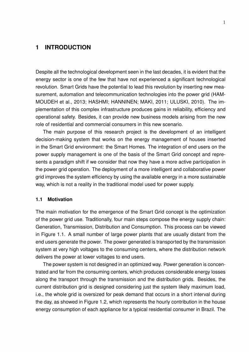
The main motivation for the emergence of the Smart Grid concept is the optimizationof the power grid use. Traditionally, four main steps compose the energy supply chain:Generation, Transmission, Distribution and Consumption. This process can be viewedin Figure 1.1. A small number of large power plants that are usually distant from theend users generate the power. The power generated is transported by the transmissionsystem at very high voltages to the consuming centers, where the distribution networkdelivers the power at lower voltages to end users.
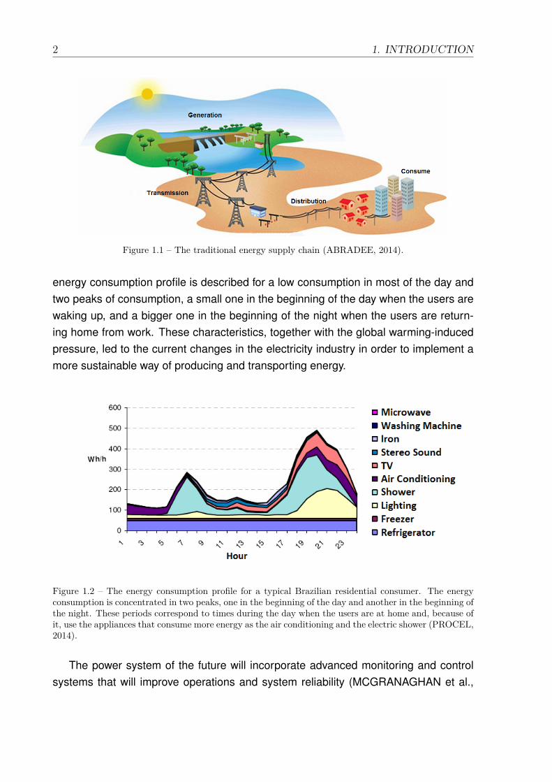
The power system is not designed in an optimized way. Power generation is concen-trated and far from the consuming centers, which produces considerable energy lossesalong the transport through the transmission and the distribution grids. Besides, thecurrent distribution grid is designed considering just the system likely maximum load,i.e., the whole grid is oversized for peak demand that occurs in a short interval duringthe day, as showed in Figure 1.2, which represents the hourly contribution in the houseenergy consumption of each appliance for a typical residential consumer in Brazil. The
2 1. INTRODUCTION
Figure 1.1 – The traditional energy supply chain (ABRADEE, 2014).
energy consumption profile is described for a low consumption in most of the day andtwo peaks of consumption, a small one in the beginning of the day when the users arewaking up, and a bigger one in the beginning of the night when the users are return-ing home from work. These characteristics, together with the global warming-inducedpressure, led to the current changes in the electricity industry in order to implement amore sustainable way of producing and transporting energy.
Figure 1.2 – The energy consumption profile for a typical Brazilian residential consumer. The energyconsumption is concentrated in two peaks, one in the beginning of the day and another in the beginning ofthe night. These periods correspond to times during the day when the users are at home and, because ofit, use the appliances that consume more energy as the air conditioning and the electric shower (PROCEL,2014).
The power system of the future will incorporate advanced monitoring and controlsystems that will improve operations and system reliability (MCGRANAGHAN et al.,
1. INTRODUCTION 3
2008). The Smart Grid concept was firstly introduced by the U.S. Department of Energyand can be defined as follows:
"Smart grid is an electricity delivery system enhanced with communicationfacilities and information technologies to enable more efficient and reliablegrid operation with an improved customer service and a cleaner environ-ment." (DOE, 2009)
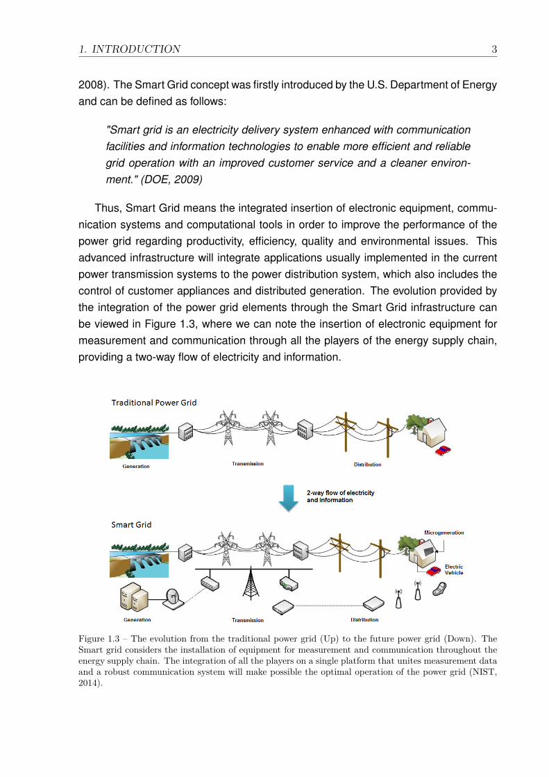
Thus, Smart Grid means the integrated insertion of electronic equipment, commu-nication systems and computational tools in order to improve the performance of thepower grid regarding productivity, efficiency, quality and environmental issues. Thisadvanced infrastructure will integrate applications usually implemented in the currentpower transmission systems to the power distribution system, which also includes thecontrol of customer appliances and distributed generation. The evolution provided bythe integration of the power grid elements through the Smart Grid infrastructure canbe viewed in Figure 1.3, where we can note the insertion of electronic equipment formeasurement and communication through all the players of the energy supply chain,providing a two-way flow of electricity and information.
Figure 1.3 – The evolution from the traditional power grid (Up) to the future power grid (Down). TheSmart grid considers the installation of equipment for measurement and communication throughout theenergy supply chain. The integration of all the players on a single platform that unites measurement dataand a robust communication system will make possible the optimal operation of the power grid (NIST,2014).

4 1. INTRODUCTION
The Smart Grid concept includes the following principles (LIU, 2010):
• Distributed Generation and Renewable Integration: Power generation pro-vided by end users and the integration of large-scale wind and solar intermittentgeneration.
• Energy Storage: Providing regulation and load shaping.
• Load Management: Making consumer demand an active tool in reducing thepeak by the implementation of Demand Response programs.
• Electric Vehicles: Lowering the greenhouse gases emission by disseminatingelectric vehicles.
• System Transparency: Seeing and operating the grid as a national system inreal-time.
• Cyber Security and Physical Security: Securing the physical infrastructure,two-way communication and data exchange.
This new scenario suggests a more active participation of consumers in the com-plete power grid management, leading to the concept of Demand Side Management(DSM) (PALENSKY; DIETRICH, 2011). This concept is related to the way consumerspay for the power use (Differentiated Energy Tariff ) and to the possibility of consumersto generate their own power (Distributed Generation), in order to provide a more opti-mized power grid operation. The management of the power supply considering the de-mand response correlates the actions of end users with the energy availability, whetheractions of energy consumption or injection into the power grid.
The effects of these changes in the distribution grid are under wide discussion, es-pecially considering the market response to the difference in the energy price for resi-dential consumers (CHEN et al., 2012; PARVANIA; FOTUHI-FIRUZABAD; SHAHIDEH-POUR, 2012; SHISHEBORI; KIAN, 2010; SU; KIRSCHEN, 2009). Traditional housesare simply power requesters, i.e., they are connected to the power grid and just re-quest the exact amount of power every time they need it. The energy flow through thepower grid follows the consumer behavior shown in Figure 1.2. In this sense, the wholepower system is oversized to meet the energy demand for a very short period, increas-ing the costs of the whole power supply chain. The Smart Grid represents an importantparadigm shift, because now consumers will contribute directly to the insertion of en-ergy into the grid, which has important technical and economic consequences.
The implementation of these new functionalities makes possible the rise of a newhouse concept that is completely integrated to the future power grid: The Smart Home.
1. INTRODUCTION 5
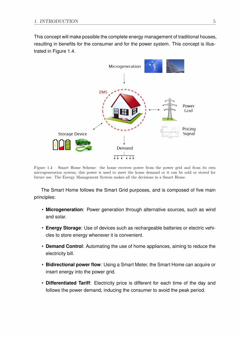
This concept will make possible the complete energy management of traditional houses,resulting in benefits for the consumer and for the power system. This concept is illus-trated in Figure 1.4.
Figure 1.4 – Smart Home Scheme: the home receives power from the power grid and from its ownmicrogeneration system; this power is used to meet the home demand or it can be sold or stored forfuture use. The Energy Management System makes all the decisions in a Smart Home.
The Smart Home follows the Smart Grid purposes, and is composed of five mainprinciples:
• Microgeneration: Power generation through alternative sources, such as windand solar.
• Energy Storage: Use of devices such as rechargeable batteries or electric vehi-cles to store energy whenever it is convenient.
• Demand Control: Automating the use of home appliances, aiming to reduce theelectricity bill.
• Bidirectional power flow: Using a Smart Meter, the Smart Home can acquire orinsert energy into the power grid.
• Differentiated Tariff: Electricity price is different for each time of the day andfollows the power demand, inducing the consumer to avoid the peak period.
6 1. INTRODUCTION
A Smart Home is described as a residential consumer that is able to generate andto store its own power. Besides, it can use electricity from the power grid or, when thepower generation exceeds the energy consumption in a given period, the consumercan still sell the surplus in the energy market, profiting with it. In this new scenario, theconsumer is also submitted to a differentiated tariff, i.e., the electricity price is higherduring the peak of demand and it is lower during the off-peak period. This economicsignal induces the residential consumer to use electricity from the power grid duringthe off-peak period and to insert energy into the power grid during the peak periodwhen the price is higher.
In this sense, considering that the energy price is variable during the day, that thegeneration through alternative sources is not constant during the day and that the con-sumer can store energy using storage devices, we can see that the decision-makingproblem involving the optimization of the house energy balance has a complex dy-namics. Thus, it is necessary to develop an autonomous decision-making system thatworks as an Energy Management System (EMS), aiming to minimize the user electric-ity bill (or to maximize the user profit) in a given period.
1.2 Objectives
A Decision-Making Support System (DMSS) (KEEN, 1980) is defined as a computer-based system that helps users to achieve specific goals in individual or organizationaldecision-making processes. In general, DMSSs help the management, planning andoperational levels, depending on the user degrees of freedom. DMSSs have found ap-plication in many areas, e.g., clinical decision support for medical diagnosis (WRIGHTA; SITTIG, 2008), business intelligence applications (POWER, 2002), agricultural pro-duction (STEPHENS; MIDDLETON, 2002), among others.
DMSS has evolved to Intelligent DMSS (IDMSS), where Artificial Intelligence (AI)concepts improve the DMSS robustness (SOL HENK G., 1987; T. JAY E., 2008). As aresult, a new set of applications emerged in different areas, increasing the importanceof those systems to solve optimization problems that are difficult to humans.
The main goal of this research is to propose a Learning-based IDMSS that aims tooptimize the power operation of a Smart Home for a given sequence of prices from theenergy market. This IDMSS works as an EMS, which learns an operation policy aimingto minimize the energy bill of a residential consumer. We propose a robust EMS thatlearns an efficient energy selling policy, even considering the lack of available data forthe learning process.
1. INTRODUCTION 7
This research also involves the study of each subsystem composing the SmartHome concept shown in Figure 1.4 and the study and application of ReinforcementLearning techniques that meet the proposed problem.
1.3 Contributions of this work
The major contribution of this research is to propose a new approach for both modelingand solving the energy management problem in Smart Homes. We propose an EMSarchitecture that obtains an efficient energy selling policy, even considering the lack ofavailable generation and price data. The EMS was tested with real energy generationand energy price data for two different places and, considering that these data havea strong dependence of location, we shown that the proposed system can be used insituations characterized by different levels of uncertainty.
The solution using Reinforcement Learning (RL) and Batch-Reinforcement Learn-ing (Batch-RL) requires the modeling of the problem as a Markov Decision Process(MDP), and one point to be discussed is how the available information is inserted intothe model, avoiding the curse of dimensionality and the increase of the problem statespace. We propose an innovative way to enter price information into the model as trendindexes, which represents a significant gain if we observe the resulting reduced statespace and the amount of information available to be considered into the model. Manyworks use only the absolute value of the price in their models, not considering the realvariation of the energy price. In particular, the results demonstrate that the modelingusing MDP (RUSSELL et al., 1996) and the solution using Batch-RL (ERNST et al.,2005a) are feasible, despite the presented limitations and the problem constraints.
The solutions proposed in the literature describe the system in a different way and,in the most cases, the tests realized do not consider real generation and price data.The solution here proposed guarantees the degree of freedom of the user, since itoptimizes the usage of energy sources considering only the price informed. Thus, theuser does not have restrictions regarding the use of appliances in his/her home. Webelieve this degree of freedom is essential so that a solution as here proposed can beincorporated into the routine of the user, leading to the popularization of systems likethis. Moreover, the proposed EMS achieves a significant result using a fixed and smallset of data, which is important for real application.
Partial results related to the development of this research led to the following publi-cations:
• "Aplicação de Aprendizado por Reforço na Otimização da Venda de En-ergia na Geração Distribuída" (BERLINK; COSTA, 2013): Article presented
8 1. INTRODUCTION
at "ENIAC 2013 - Encontro Nacional de Inteligência Artificial e Computacional",when a simplified version of the Smart Home energy management problem weresolved by using the Q-Learning algorithm;
• "Intelligent Decision-Making for Smart Home Energy Management" (BERLINK;KAGAN; COSTA, 2014): Article submitted to "JRIS - Journal of Robotics and In-telligent Systems" and published in 2014, where the first version of the Reinforcement-Learning based Energy Management System (RLbEMS) proposed in this re-search were presented.
1.4 Organization
In order to detail the proposed research, this document is organized as follows:
• Chapter 2 – Problem Statement states the problem assumptions, describing themodels considered for each subsystem of the proposed problem. Also, definesthe set of premises and the main restrictions regarding the problem solution.
• Chapter 3 – Intelligent Energy Management in Smart Homes provides theliterature review about how the energy management in Smart Homes problemhas been solved and explains the solution proposed in this research;
• Chapter 4 – Background covers the mathematical framework and the theoreticalconcepts used to implement the solution proposed in this research;
• Chapter 5 – Reinforcement Learning Based EMS for Smart Homes explainsthe modeling and how the background were used to implement the proposedEMS. Besides, presents the EMS algorithms and how it operates at runtime.
• Chapter 6 – Experimental Results shows the obtained results and discuss theCase Studies of the research. Also, discuss if the proposed solution meets thepremises and constraints defined before.
• Chapter 7 – Conclude highlights the impacts of the research and presents thenext steps.
9
2 PROBLEM STATEMENT
Figure 1.4 shows a scheme of a Smart Home EMS that makes decisions based onfour main variables: the current energy generation, the energy storage level, the houseenergy demand and the current electricity price. The objective of this section is todiscuss each of these subsystems in further detail. In addition, we discuss the modelsadopted for each subsystem involved in the Smart Home EMS development.
2.1 Residential Demand Response
Demand Response (DR) is commonly defined as changes in electric usage by end-use customers from their normal consumption patterns in response to changes in theprice of electricity over time, or to incentives through payments in order to induce lowerelectricity use at times of high wholesale market prices or when system reliability isjeopardized (BALIJEPALLI et al., 2011).
Historically, this concept were used in contingency situations, as happened in Brazilduring the energy crisis in 2001. In that time, the government imposed a surtax on en-ergy bills that were greater than 200 kWh per month. The consumer had to pay 50%more on the amount that exceed this level. In addition, there were a second surtaxof 200% for bills above 500 kWh per month. This program results in a decrease ofmore than 20% of energy consumption in the period, being known as one of the mostsuccessful demand response programs implemented to date (WATTS; ARIZTIA, 2002;JARDINI et al., 2002). Nowadays, this concept is implemented preventively, trying toavoid situations as the experimented in 2001 in Brazil. Demand Response Programs(DRP) are being implemented in many places and under different configurations, al-ways aiming to optimize the power grid by inducing the energy use of consumers.
While inserted in DRP, consumers can act in a passive or active way. Passive con-sumers are those who just change their consumption pattern by modifying the amountand time of energy use from the power grid; active consumers are those who, besideschanging the amount and time of energy use, insert energy into the power grid fol-lowing a price signal. This concept is only possible because of the Smart-Meteringand Information Technology infrastructure implemented by Smart Grids (ALBADI; EL-SAADANY, 2007).
10 2. PROBLEM STATEMENT
In this new scenario, the consumer can also act as an energy trader, selling energyin a convenient way to the utility company. If this process is conducted in an optimizedway, consumers can meet their demand and even profit at the end of a given period.
The problem investigated in this research considers active consumers inserted inthe Smart Grid system. The consumers have their own power generation throughalternative sources and have a storage device. The power generated can be solddirectly to the energy market at the current price, can be used to meet the housedemand or can be placed in the storage device to be used or sold at a convenientfuture time.
The solution we propose in this work keeps the user freedom in decisions aboutenergy consumption, i.e., we promote a demand response without changing its con-sumption profile. This assumption results in an advantage for the user, since the resultsdo not take into account the change of his/her way of consuming energy. We modela decision process that does not consider as control action any interference in theconsumption profile of the user.
The DR is the concept that makes possible the development of a real integrated andenergy efficient Smart Home. It creates an incentive for users to change their energyusage pattern, whether by changing the energy consumption profile or by using an-other power supply to compensate the energy consumption in inappropriate periods.Considering that energy prices reflect the energy availability in the market, the con-sumers will now contribute directly for the regularization of the system, improving thesystem stability and reducing the costs of utilities to keep the power distribution grid.
2.2 Energy Microgeneration
Alternative methods of generating power through renewable sources differ in manyways from conventional methods of power production. As conventional methods, themost commonly used are those that use the combustion of fossil fuels (Thermoelectric)or the kinetic energy of water (Hydroelectric) to generate power. These alternativeways of producing electricity became very popular recently, following a sustainableappeal that has as fundamental basis the low environmental impact. However, thesesources have low capacity of production and a high cost compared with conventionalmethods. In addition, alternative power sources have in common a strong dependenceon specific weather conditions for generation, which varies considerably during the day.One of the main purposes of an EMS is to deal with this intermittence, improving theenergy utilization during the day.
Considering the alternative methods available today, solar and wind energy aremore suitable for application in residential systems due to their easy implementation

2. PROBLEM STATEMENT 11
and integration to urban architecture. However, the solar photovoltaic technology ismostly used considering that it is more difficult to find an urban spot with great potentialfor wind power. Solar power is also more regular and can be predicted in an easier way;we usually have a peak of generation in the middle of the day for solar technology anda completely variable generation profile for wind technology. Because of its higher levelof penetration, we consider a Smart Home with this kind of power generation.
Technically, there are several ways of using solar power to produce electricity. Thesolar photovoltaic technology is the most popular one, because of its easy implementa-tion, flexibility and direct conversion of solar energy into electricity, without any interme-diate stages. The solar photovoltaic panels are composed of solar cells that captureenergy from the light (natural or artificial) and create an electric potential differencebecause of the photovoltaic effect. The photovoltaic effect was discovered during the19th century, but became popular in 1904 when Albert Einstein published an articleexplaining its physical nature and, because of it, earned his Nobel Prize.
The electric potential created by the solar cells generates an electric flow when con-nected to a load, which is the basis of the power supply by using this energy source.The electric current generated by the solar panels is direct, differing from the alternat-ing current commonly used in residential systems. Hence, a set of equipment, suchas inverters, load controllers and others are used to implement this technology. Thecomplete system can be viewed in Figure 2.1.
Figure 2.1 – Complete solar photovoltaic system applied to a common residence in a connected way. Thereal application (Left) and the components of the system (Right) are presented (NEOSOLAR, 2014).
This technology can be applied in a connected or isolated way. The connectedsystems are those that are integrated to the Smart Grid, being able to insert powerwhenever possible; the isolated systems are used in residences far from the consumingcenters and must use batteries to deal with the intermittency of the energy source. Inthis work, we consider a connected Solar Photovoltaic System (Solar PV System).
As stated before, the alternative ways of producing energy have a strong depen-dence on specific weather conditions. The energy generation through solar systems
12 2. PROBLEM STATEMENT
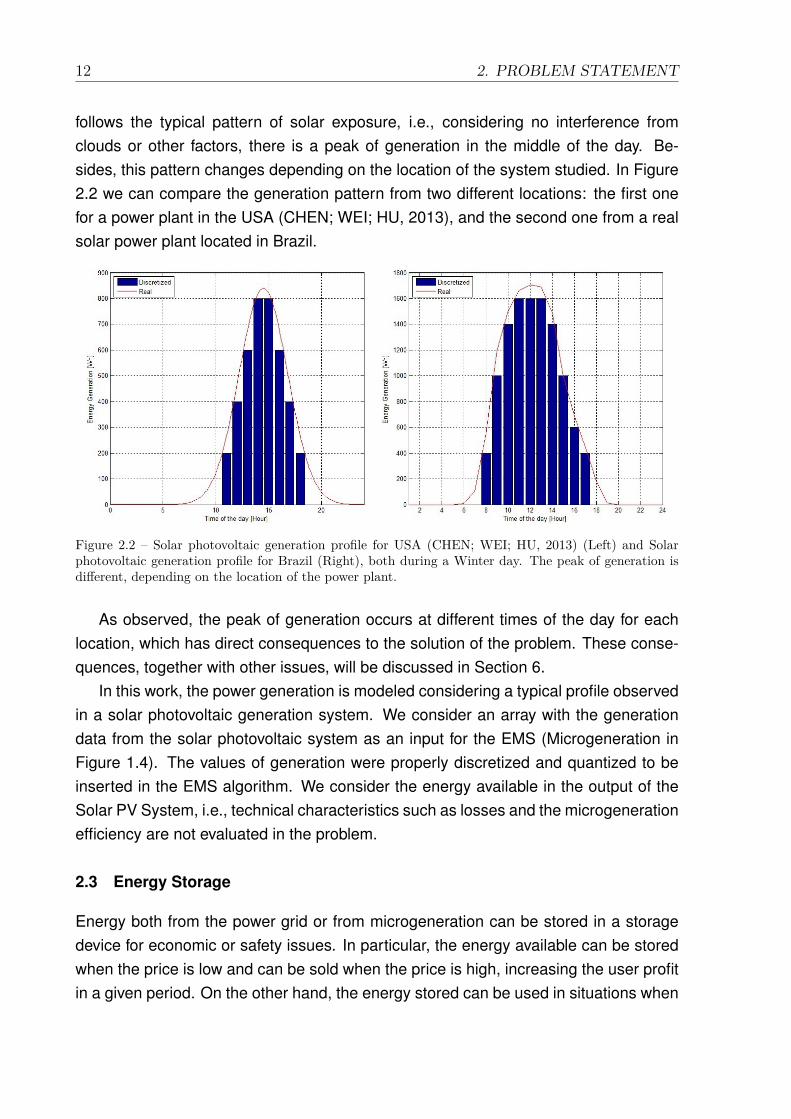
follows the typical pattern of solar exposure, i.e., considering no interference fromclouds or other factors, there is a peak of generation in the middle of the day. Be-sides, this pattern changes depending on the location of the system studied. In Figure2.2 we can compare the generation pattern from two different locations: the first onefor a power plant in the USA (CHEN; WEI; HU, 2013), and the second one from a realsolar power plant located in Brazil.
Figure 2.2 – Solar photovoltaic generation profile for USA (CHEN; WEI; HU, 2013) (Left) and Solarphotovoltaic generation profile for Brazil (Right), both during a Winter day. The peak of generation isdifferent, depending on the location of the power plant.
As observed, the peak of generation occurs at different times of the day for eachlocation, which has direct consequences to the solution of the problem. These conse-quences, together with other issues, will be discussed in Section 6.
In this work, the power generation is modeled considering a typical profile observedin a solar photovoltaic generation system. We consider an array with the generationdata from the solar photovoltaic system as an input for the EMS (Microgeneration inFigure 1.4). The values of generation were properly discretized and quantized to beinserted in the EMS algorithm. We consider the energy available in the output of theSolar PV System, i.e., technical characteristics such as losses and the microgenerationefficiency are not evaluated in the problem.
2.3 Energy Storage
Energy both from the power grid or from microgeneration can be stored in a storagedevice for economic or safety issues. In particular, the energy available can be storedwhen the price is low and can be sold when the price is high, increasing the user profitin a given period. On the other hand, the energy stored can be used in situations when

2. PROBLEM STATEMENT 13
there is no available energy from the power grid or from the microgeneration, keepingthe energy supply for at least part of the house demand in a given period.
The storage device is one of the most important elements of Smart Homes and,despite the growing application in houses nowadays, it is still the most expensive(CARPINELLI et al., 2013; WANG et al., 2013). Considering that, special care must betaken about the specification of this device, otherwise the profit from the sale of energywill not make up for the investment.
In general, we consider the rechargeable batteries and electric vehicles as resi-dential storage devices. The main difference between them is the availability, becausewhile the battery is always available for use, electric vehicles will not be available whenthey leave the house. These systems can be viewed in Figure 2.3. In this research, weconsider just a set of rechargeable batteries as storage device.
Figure 2.3 – Storage devices commonly used in residential systems. Set of rechargeable batteries (Left)and Electric Vehicle (Right). (MPPTSOLAR, 2014)
There are several ways to model the charging and discharging of a battery, de-pending on the application and the type of the used battery. In this work, we usedthe storage model proposed by Atzeni et al. (2013). The main characteristics of thesedevices are the charge and discharge efficiency, β+ and β−, the maximum chargingand discharging rate, smax, rate of energy loss over time, αB, and maximum storagecapacity, BMAX .
The EMS acquire, for each discrete instant k, the measure of the charge levelthrough a energy meter installed in the battery. The value of the charge level, b(k),is then inserted into a quantizer. The quantized charge level, B(k), is the value that isinserted into the EMS algorithm.
We define s+(k) and s−(k) as the charge and discharge of the battery for eachinstant k, respectively. For each instant k:
s+(k) ≥ 0. (2.1)

14 2. PROBLEM STATEMENT
s−(k) ≤ 0. (2.2)
As exposed before, we also define β+ and β− as the charge and discharge effi-ciency, respectively. Considering this:
0 < β+ ≤ 1, (2.3)
β− ≥ 1. (2.4)
We also define the leakage rate, αB, that indicates the energy loss over time. Forthis parameter, we have:
0 < αB ≤ 1. (2.5)
Considering this, we can describe the dynamic of battery charge and discharge as:
b(k) = αB.b(k − 1) + β′.s(k), (2.6)
where:
s(k) = (s+(k), s−(k))′, (2.7)
and:
β = (β+, β−)′. (2.8)
Besides, we define the maximum charge and discharge rate, smax. This parametermust be observed carefully, in order to consider the battery restrictions in the solutionof the problem. So:
β′s(k) ≤ smax. (2.9)
As exposed, into the algorithm the battery is represented as a discretized and quan-tized variable, B(k), limited by the maximum storage capacity, BMAX , which increasesits value when the EMS chooses to store the surplus of the generated power. Thevalues of B(k) belong to the set {0, QZ , 2.QZ , ..., BMAX}, where QZ refers to the quan-tization level used in this work. The quantization process will be described fully in thefollowing sections. In our model, B(k) = 0 means that there is no energy in the batteryand B(k) = BMAX means that the battery is full. The battery stores energy with the
2. PROBLEM STATEMENT 15
same quantization levels used for the energy generated by the microgeneration systemand for the energy consumed by the Smart Home.
The maximum storage capacity of the battery affects the EMS degree of freedom tochoose actions. Note that there are always more admissible actions to choose in eachstate of operation when batteries with higher capacities are used. However, increasingthe battery capacity makes the system more expensive. A point to be considered is therestriction imposed by the maximum charge and discharge. This restriction limits theamount of energy that can be sold or used from the battery. Because of it, the EMSmust evaluate if, in each instant k, it is a good option to storage energy considering thatin the future it will not be able to sell all the available energy, eventually. It is importantto mention that, usually, the maximum charge and discharge rate is proportional toBMAX , i.e., this parameters are directly related.
In this work, we consider a simplified version of the model proposed by (ATZENIet al., 2013). We used a lithium-ion battery with αB = 24
√0.9, β+ = 0.9, β− = 1.1,
BMAX = 4kWh and smax = 2kW , which corresponds to charge or discharge 2kWh ofenergy each hour. Besides, we consider for discretization a period (T) of one hour, i.e.,the measures from the energy meters are realized in each hour.
In this research, we also evaluated the influence of the Maximum Storage Capacity,BMAX , on the operation of the proposed EMS.
2.4 Energy Demand
The energy demand considers the electrical energy consumed by the user’s appli-ances. The energy consumed by a common house usually follows a typical profile asthe one presented in Figure 1.2. This profile is related to the quantity of consumersin the house, the quantity of electrical appliances and others specific characteristics.Besides, it is directly related to the house location. Considering that appliances relatedto warming, as heaters, or to cooling, as air conditioners, are the ones that consumemore energy, houses located in places with a hot or cold weather may have a differentenergy consumption profile.
This work considers a Smart Home that has the same electrical appliances as a typ-ical house. We consider a house monitored by a energy meter that is able to measurethe energy consumption, d(k), in each hour. The measure is inserted into a quantizer,that uses the same quantization levels of the others subsystems. Then, the discreteand quantized energy consumption measure, D(k), is inserted into the EMS algorithm.This value will compose the Smart Home energetic state, the same way as the genera-tion, storage and price information. The modeling and state definition will be discussedin detail in Section 5.
16 2. PROBLEM STATEMENT
One objective of this work is to evaluate the proposed EMS using real data forall subsystems considered in the Smart Home. Our work considers a Smart Homeinserted in the Smart Grid scenario, which involves the use of Smart Meters to measurethe residential energy consumption for each hour. However, the Smart Grid is a newconcept and, at this point, it is difficult to obtain these data from utilities. Consideringthis, we chose to develop a methodology to generate the energy consumption data fora house, considering the most common electrical appliances used and the behavior ofa typical consumer. Although the consumption data were not actually measured, themethodology used results in a consumption profile that is very close to the consumptionof a real house, which supports the analysis of the results obtained during the tests.
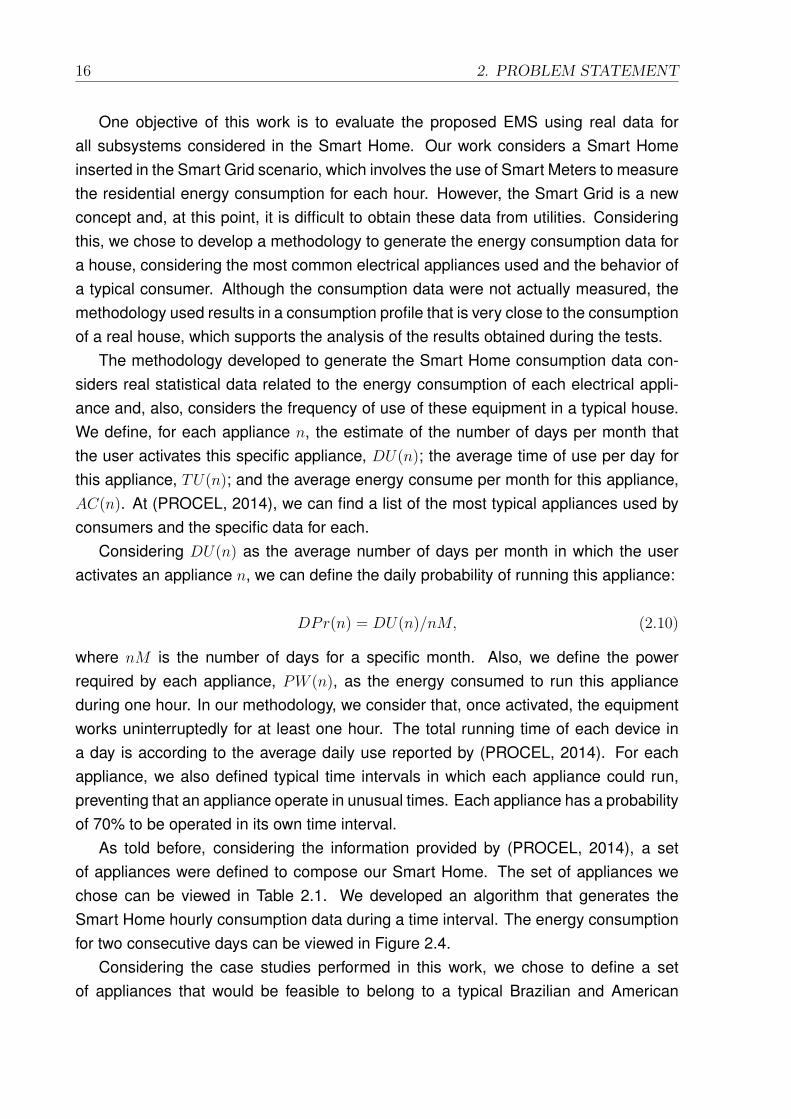
The methodology developed to generate the Smart Home consumption data con-siders real statistical data related to the energy consumption of each electrical appli-ance and, also, considers the frequency of use of these equipment in a typical house.We define, for each appliance n, the estimate of the number of days per month thatthe user activates this specific appliance, DU(n); the average time of use per day forthis appliance, TU(n); and the average energy consume per month for this appliance,AC(n). At (PROCEL, 2014), we can find a list of the most typical appliances used byconsumers and the specific data for each.
Considering DU(n) as the average number of days per month in which the useractivates an appliance n, we can define the daily probability of running this appliance:
DPr(n) = DU(n)/nM, (2.10)
where nM is the number of days for a specific month. Also, we define the powerrequired by each appliance, PW (n), as the energy consumed to run this applianceduring one hour. In our methodology, we consider that, once activated, the equipmentworks uninterruptedly for at least one hour. The total running time of each device ina day is according to the average daily use reported by (PROCEL, 2014). For eachappliance, we also defined typical time intervals in which each appliance could run,preventing that an appliance operate in unusual times. Each appliance has a probabilityof 70% to be operated in its own time interval.
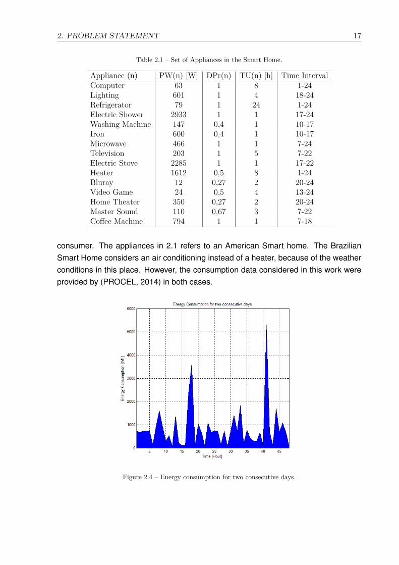
As told before, considering the information provided by (PROCEL, 2014), a setof appliances were defined to compose our Smart Home. The set of appliances wechose can be viewed in Table 2.1. We developed an algorithm that generates theSmart Home hourly consumption data during a time interval. The energy consumptionfor two consecutive days can be viewed in Figure 2.4.
Considering the case studies performed in this work, we chose to define a setof appliances that would be feasible to belong to a typical Brazilian and American
2. PROBLEM STATEMENT 17
Table 2.1 – Set of Appliances in the Smart Home.
Appliance (n) PW(n) [W] DPr(n) TU(n) [h] Time IntervalComputer 63 1 8 1-24Lighting 601 1 4 18-24Refrigerator 79 1 24 1-24Electric Shower 2933 1 1 17-24Washing Machine 147 0,4 1 10-17Iron 600 0,4 1 10-17Microwave 466 1 1 7-24Television 203 1 5 7-22Electric Stove 2285 1 1 17-22Heater 1612 0,5 8 1-24Bluray 12 0,27 2 20-24Video Game 24 0,5 4 13-24Home Theater 350 0,27 2 20-24Master Sound 110 0,67 3 7-22Coffee Machine 794 1 1 7-18
consumer. The appliances in 2.1 refers to an American Smart home. The BrazilianSmart Home considers an air conditioning instead of a heater, because of the weatherconditions in this place. However, the consumption data considered in this work wereprovided by (PROCEL, 2014) in both cases.
Figure 2.4 – Energy consumption for two consecutive days.

18 2. PROBLEM STATEMENT
Comparing Figure 1.2 and Figure 2.4 we can verify that the application of thismethodology results in a consumption profile that is very close to reality. This sim-ilarity can be clearly seen by the peak consumption in the evening and by the lowpower consumption throughout the day. Before getting into the EMS, these data areinserted into a quantizer that uses the same quantization levels of the generation andstorage data. This data will be used to compose the system energetic state.
2.5 Energy Pricing Models
As stated in Section 2.1, Demand Response Programs (DRP) are being implementedin several places in the world in order to promote a greater participation of end usersin the efficient use of the available energy. DRP are implemented aiming at regulatingboth demand control, through the differentiated tariffs, such as the insertion of energyin the network, by rewarding the consumer for the produced energy.
There are two common ways of implementing demand control (PALENSKY; DIET-RICH, 2011): the Incentive-Based Demand Response (Table 2.1) and the Time-BasedRates Demand Response (Table 2.2). We also describe DRP as Direct or Indirect.Direct DRP are those that change the consumption pattern by a direct actuation in theconsumer’s demand. They differ from Indirect DRP that use economic signals in orderto induce the changes in the consumption pattern, such as the differentiated tariffs.We will focus on the Indirect DRP, because they are easy to implement and producegreater gains in the long-term, considering that they act on the consumer behavior ofhow and when using energy.
Table 2.2 – Direct or Incentive-Based Demand Response Programs: Types and descriptions.
Direct load control Utility or grid operator gets freeaccess to customer processes.
Interruptible/curtailable rates Customers get special contractwith limited sheds.
Emergency DR programs Voluntary response to emergencysignals.
Capacity market programs Customers guarantee to pitch inwhen the grid is in need.
Demand bidding programs Customers can bid for curtailingat attractive prices.
The insertion of energy in the power grid may reward the end user in two ways:Feed-in Tariffs, when the end user receives a financial reward by the energy inserted inthe grid, and Net-Metering, when the end user just accumulates a credit by the energy
2. PROBLEM STATEMENT 19
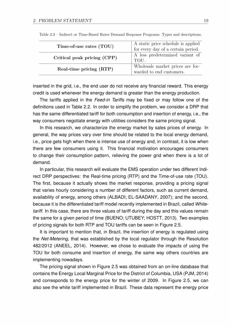
Table 2.3 – Indirect or Time-Based Rates Demand Response Programs: Types and descriptions.
Time-of-use rates (TOU) A static price schedule is appliedfor every day of a certain period.
Critical peak pricing (CPP) A less predetermined variant ofTOU.
Real-time pricing (RTP) Wholesale market prices are for-warded to end customers.
inserted in the grid, i.e., the end user do not receive any financial reward. This energycredit is used whenever the energy demand is greater than the energy production.
The tariffs applied in the Feed-in Tariffs may be fixed or may follow one of thedefinitions used in Table 2.2. In order to simplify the problem, we consider a DRP thathas the same differentiated tariff for both consumption and insertion of energy, i.e., theway consumers negotiate energy with utilities considers the same pricing signal.
In this research, we characterize the energy market by sales prices of energy. Ingeneral, the way prices vary over time should be related to the local energy demand,i.e., price gets high when there is intense use of energy and, in contrast, it is low whenthere are few consumers using it. This financial motivation encourages consumersto change their consumption pattern, relieving the power grid when there is a lot ofdemand.
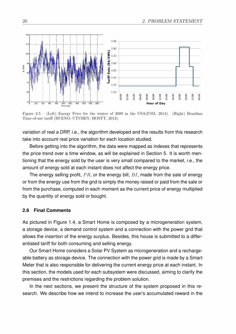
In particular, this research will evaluate the EMS operation under two different Indi-rect DRP perspectives: the Real-time pricing (RTP) and the Time-of-use rate (TOU).The first, because it actually shows the market response, providing a pricing signalthat varies hourly considering a number of different factors, such as current demand,availability of energy, among others (ALBADI; EL-SAADANY, 2007); and the second,because it is the differentiated tariff model recently implemented in Brazil, called White-tariff. In this case, there are three values of tariff during the day and this values remainthe same for a given period of time (BUENO; UTUBEY; HOSTT, 2013). Two examplesof pricing signals for both RTP and TOU tariffs can be seen in Figure 2.5.
It is important to mention that, in Brazil, the insertion of energy is regulated usingthe Net-Metering, that was established by the local regulator through the Resolution482/2012 (ANEEL, 2014). However, we chose to evaluate the impacts of using theTOU for both consume and insertion of energy, the same way others countries areimplementing nowadays.
The pricing signal shown in Figure 2.5 was obtained from an on-line database thatcontains the Energy Local Marginal Price for the District of Columbia, USA (PJM, 2014)and corresponds to the energy price for the winter of 2009. In Figure 2.5, we canalso see the white tariff implemented in Brazil. These data represent the energy price
20 2. PROBLEM STATEMENT
Figure 2.5 – (Left) Energy Price for the winter of 2009 in the USA(PJM, 2014). (Right) BrazilianTime-of-use tariff (BUENO; UTUBEY; HOSTT, 2013).
variation of real a DRP, i.e., the algorithm developed and the results from this researchtake into account real price variation for each location studied.
Before getting into the algorithm, the data were mapped as indexes that representsthe price trend over a time window, as will be explained in Section 5. It is worth men-tioning that the energy sold by the user is very small compared to the market, i.e., theamount of energy sold at each instant does not affect the energy price.
The energy selling profit, PR, or the energy bill, BI, made from the sale of energyor from the energy use from the grid is simply the money raised or paid from the sale orfrom the purchase, computed in each moment as the current price of energy multipliedby the quantity of energy sold or bought.
2.6 Final Comments
As pictured in Figure 1.4, a Smart Home is composed by a microgeneration system,a storage device, a demand control system and a connection with the power grid thatallows the insertion of the energy surplus. Besides, this house is submitted to a differ-entiated tariff for both consuming and selling energy.
Our Smart Home considers a Solar PV System as microgeneration and a recharge-able battery as storage device. The connection with the power grid is made by a SmartMeter that is also responsible for delivering the current energy price at each instant. Inthis section, the models used for each subsystem were discussed, aiming to clarify thepremises and the restrictions regarding the problem solution.
In the next sections, we present the structure of the system proposed in this re-search. We describe how we intend to increase the user’s accumulated reward in the

2. PROBLEM STATEMENT 21
long-term, respecting the premises and restrictions here described. Besides, we de-scribe the two case studies performed in this work, when was possible to attest thesystem effectiveness.

22 2. PROBLEM STATEMENT
23
3 INTELLIGENT ENERGY MANAGEMENT IN SMART HOMES
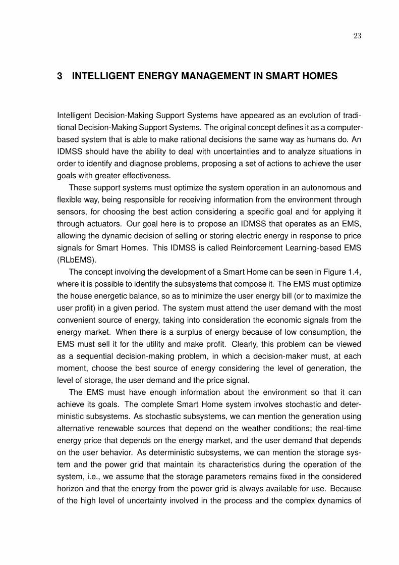
Intelligent Decision-Making Support Systems have appeared as an evolution of tradi-tional Decision-Making Support Systems. The original concept defines it as a computer-based system that is able to make rational decisions the same way as humans do. AnIDMSS should have the ability to deal with uncertainties and to analyze situations inorder to identify and diagnose problems, proposing a set of actions to achieve the usergoals with greater effectiveness.
These support systems must optimize the system operation in an autonomous andflexible way, being responsible for receiving information from the environment throughsensors, for choosing the best action considering a specific goal and for applying itthrough actuators. Our goal here is to propose an IDMSS that operates as an EMS,allowing the dynamic decision of selling or storing electric energy in response to pricesignals for Smart Homes. This IDMSS is called Reinforcement Learning-based EMS(RLbEMS).
The concept involving the development of a Smart Home can be seen in Figure 1.4,where it is possible to identify the subsystems that compose it. The EMS must optimizethe house energetic balance, so as to minimize the user energy bill (or to maximize theuser profit) in a given period. The system must attend the user demand with the mostconvenient source of energy, taking into consideration the economic signals from theenergy market. When there is a surplus of energy because of low consumption, theEMS must sell it for the utility and make profit. Clearly, this problem can be viewedas a sequential decision-making problem, in which a decision-maker must, at eachmoment, choose the best source of energy considering the level of generation, thelevel of storage, the user demand and the price signal.
The EMS must have enough information about the environment so that it canachieve its goals. The complete Smart Home system involves stochastic and deter-ministic subsystems. As stochastic subsystems, we can mention the generation usingalternative renewable sources that depend on the weather conditions; the real-timeenergy price that depends on the energy market, and the user demand that dependson the user behavior. As deterministic subsystems, we can mention the storage sys-tem and the power grid that maintain its characteristics during the operation of thesystem, i.e., we assume that the storage parameters remains fixed in the consideredhorizon and that the energy from the power grid is always available for use. Becauseof the high level of uncertainty involved in the process and the complex dynamics of
24 3. INTELLIGENT ENERGY MANAGEMENT IN SMART HOMES
the Smart Home subsystems, we propose a learning-based EMS, making the systemrobust to the high level of uncertainty on the environment dynamics.
In the following sections, some related work is presented. We will see that there aremany different ways to model and to solve this problem, depending on the optimizationobjectives and on the assumptions and restrictions of each proposal. The operationstrategy and the EMS architecture adopted in this research are also presented.
3.1 Related Work
In computing and power systems community, many researchers have developed opti-mization algorithms to deal with the energy management of Smart Homes. The inte-gration of the local energy management on houses and the global energy managementof the power distribution grid can be analyzed under different perspectives.
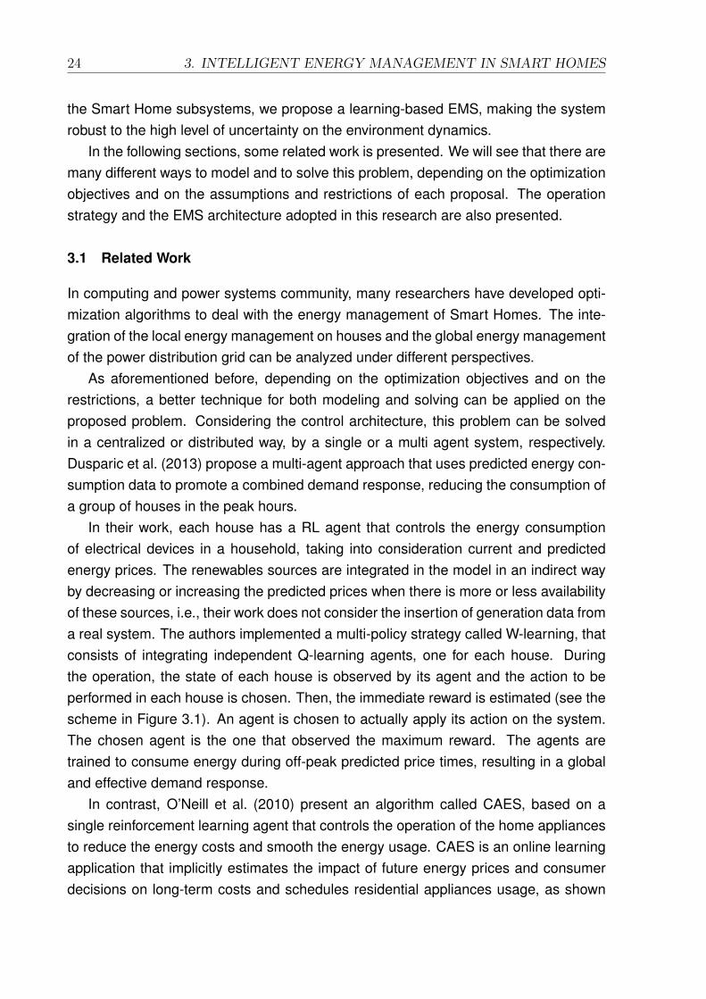
As aforementioned before, depending on the optimization objectives and on therestrictions, a better technique for both modeling and solving can be applied on theproposed problem. Considering the control architecture, this problem can be solvedin a centralized or distributed way, by a single or a multi agent system, respectively.Dusparic et al. (2013) propose a multi-agent approach that uses predicted energy con-sumption data to promote a combined demand response, reducing the consumption ofa group of houses in the peak hours.
In their work, each house has a RL agent that controls the energy consumptionof electrical devices in a household, taking into consideration current and predictedenergy prices. The renewables sources are integrated in the model in an indirect wayby decreasing or increasing the predicted prices when there is more or less availabilityof these sources, i.e., their work does not consider the insertion of generation data froma real system. The authors implemented a multi-policy strategy called W-learning, thatconsists of integrating independent Q-learning agents, one for each house. Duringthe operation, the state of each house is observed by its agent and the action to beperformed in each house is chosen. Then, the immediate reward is estimated (see thescheme in Figure 3.1). An agent is chosen to actually apply its action on the system.The chosen agent is the one that observed the maximum reward. The agents aretrained to consume energy during off-peak predicted price times, resulting in a globaland effective demand response.
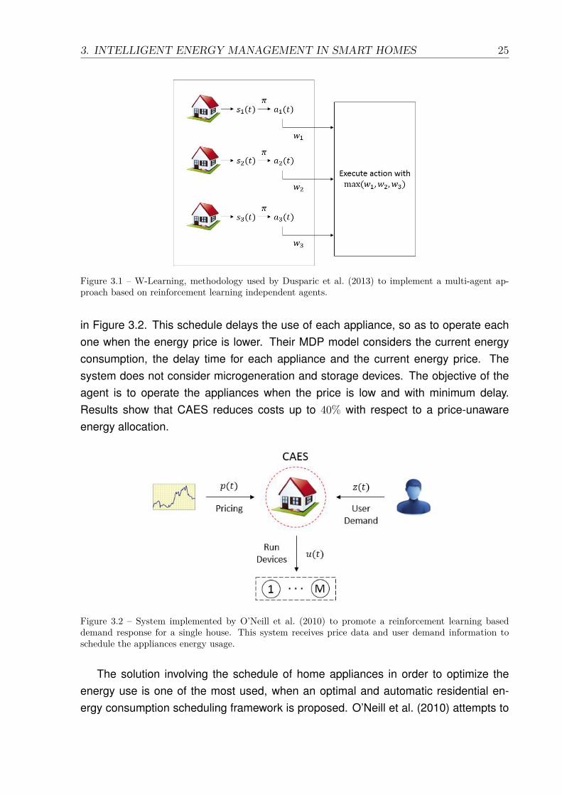
In contrast, O’Neill et al. (2010) present an algorithm called CAES, based on asingle reinforcement learning agent that controls the operation of the home appliancesto reduce the energy costs and smooth the energy usage. CAES is an online learningapplication that implicitly estimates the impact of future energy prices and consumerdecisions on long-term costs and schedules residential appliances usage, as shown
3. INTELLIGENT ENERGY MANAGEMENT IN SMART HOMES 25
Figure 3.1 – W-Learning, methodology used by Dusparic et al. (2013) to implement a multi-agent ap-proach based on reinforcement learning independent agents.
in Figure 3.2. This schedule delays the use of each appliance, so as to operate eachone when the energy price is lower. Their MDP model considers the current energyconsumption, the delay time for each appliance and the current energy price. Thesystem does not consider microgeneration and storage devices. The objective of theagent is to operate the appliances when the price is low and with minimum delay.Results show that CAES reduces costs up to 40% with respect to a price-unawareenergy allocation.
Figure 3.2 – System implemented by O’Neill et al. (2010) to promote a reinforcement learning baseddemand response for a single house. This system receives price data and user demand information toschedule the appliances energy usage.
The solution involving the schedule of home appliances in order to optimize theenergy use is one of the most used, when an optimal and automatic residential en-ergy consumption scheduling framework is proposed. O’Neill et al. (2010) attempts to
26 3. INTELLIGENT ENERGY MANAGEMENT IN SMART HOMES
achieve a desired trade-off between minimizing the electricity payment and minimizingthe waiting time for the operation of each appliance, which is important to minimize theinterference of the system operation on the user’s comfort.
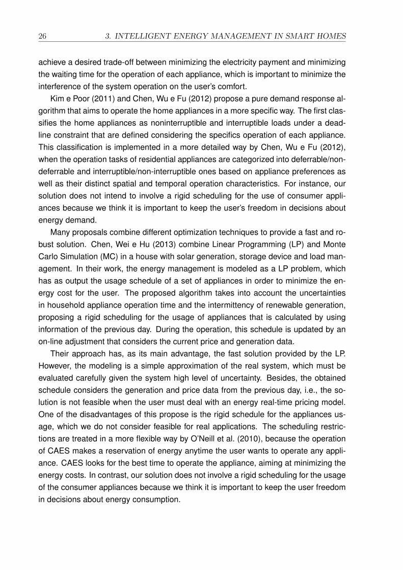
Kim e Poor (2011) and Chen, Wu e Fu (2012) propose a pure demand response al-gorithm that aims to operate the home appliances in a more specific way. The first clas-sifies the home appliances as noninterruptible and interruptible loads under a dead-line constraint that are defined considering the specifics operation of each appliance.This classification is implemented in a more detailed way by Chen, Wu e Fu (2012),when the operation tasks of residential appliances are categorized into deferrable/non-deferrable and interruptible/non-interruptible ones based on appliance preferences aswell as their distinct spatial and temporal operation characteristics. For instance, oursolution does not intend to involve a rigid scheduling for the use of consumer appli-ances because we think it is important to keep the user’s freedom in decisions aboutenergy demand.
Many proposals combine different optimization techniques to provide a fast and ro-bust solution. Chen, Wei e Hu (2013) combine Linear Programming (LP) and MonteCarlo Simulation (MC) in a house with solar generation, storage device and load man-agement. In their work, the energy management is modeled as a LP problem, whichhas as output the usage schedule of a set of appliances in order to minimize the en-ergy cost for the user. The proposed algorithm takes into account the uncertaintiesin household appliance operation time and the intermittency of renewable generation,proposing a rigid scheduling for the usage of appliances that is calculated by usinginformation of the previous day. During the operation, this schedule is updated by anon-line adjustment that considers the current price and generation data.
Their approach has, as its main advantage, the fast solution provided by the LP.However, the modeling is a simple approximation of the real system, which must beevaluated carefully given the system high level of uncertainty. Besides, the obtainedschedule considers the generation and price data from the previous day, i.e., the so-lution is not feasible when the user must deal with an energy real-time pricing model.One of the disadvantages of this propose is the rigid schedule for the appliances us-age, which we do not consider feasible for real applications. The scheduling restric-tions are treated in a more flexible way by O’Neill et al. (2010), because the operationof CAES makes a reservation of energy anytime the user wants to operate any appli-ance. CAES looks for the best time to operate the appliance, aiming at minimizing theenergy costs. In contrast, our solution does not involve a rigid scheduling for the usageof the consumer appliances because we think it is important to keep the user freedomin decisions about energy consumption.
3. INTELLIGENT ENERGY MANAGEMENT IN SMART HOMES 27
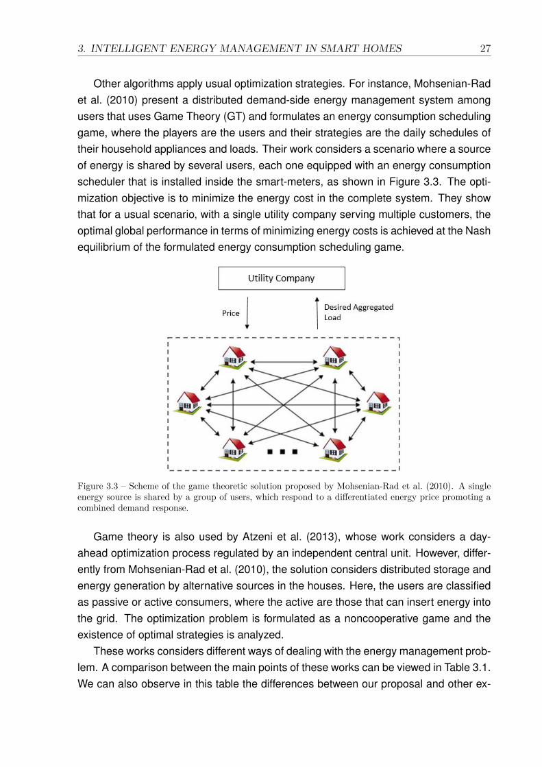
Other algorithms apply usual optimization strategies. For instance, Mohsenian-Radet al. (2010) present a distributed demand-side energy management system amongusers that uses Game Theory (GT) and formulates an energy consumption schedulinggame, where the players are the users and their strategies are the daily schedules oftheir household appliances and loads. Their work considers a scenario where a sourceof energy is shared by several users, each one equipped with an energy consumptionscheduler that is installed inside the smart-meters, as shown in Figure 3.3. The opti-mization objective is to minimize the energy cost in the complete system. They showthat for a usual scenario, with a single utility company serving multiple customers, theoptimal global performance in terms of minimizing energy costs is achieved at the Nashequilibrium of the formulated energy consumption scheduling game.
Figure 3.3 – Scheme of the game theoretic solution proposed by Mohsenian-Rad et al. (2010). A singleenergy source is shared by a group of users, which respond to a differentiated energy price promoting acombined demand response.
Game theory is also used by Atzeni et al. (2013), whose work considers a day-ahead optimization process regulated by an independent central unit. However, differ-ently from Mohsenian-Rad et al. (2010), the solution considers distributed storage andenergy generation by alternative sources in the houses. Here, the users are classifiedas passive or active consumers, where the active are those that can insert energy intothe grid. The optimization problem is formulated as a noncooperative game and theexistence of optimal strategies is analyzed.
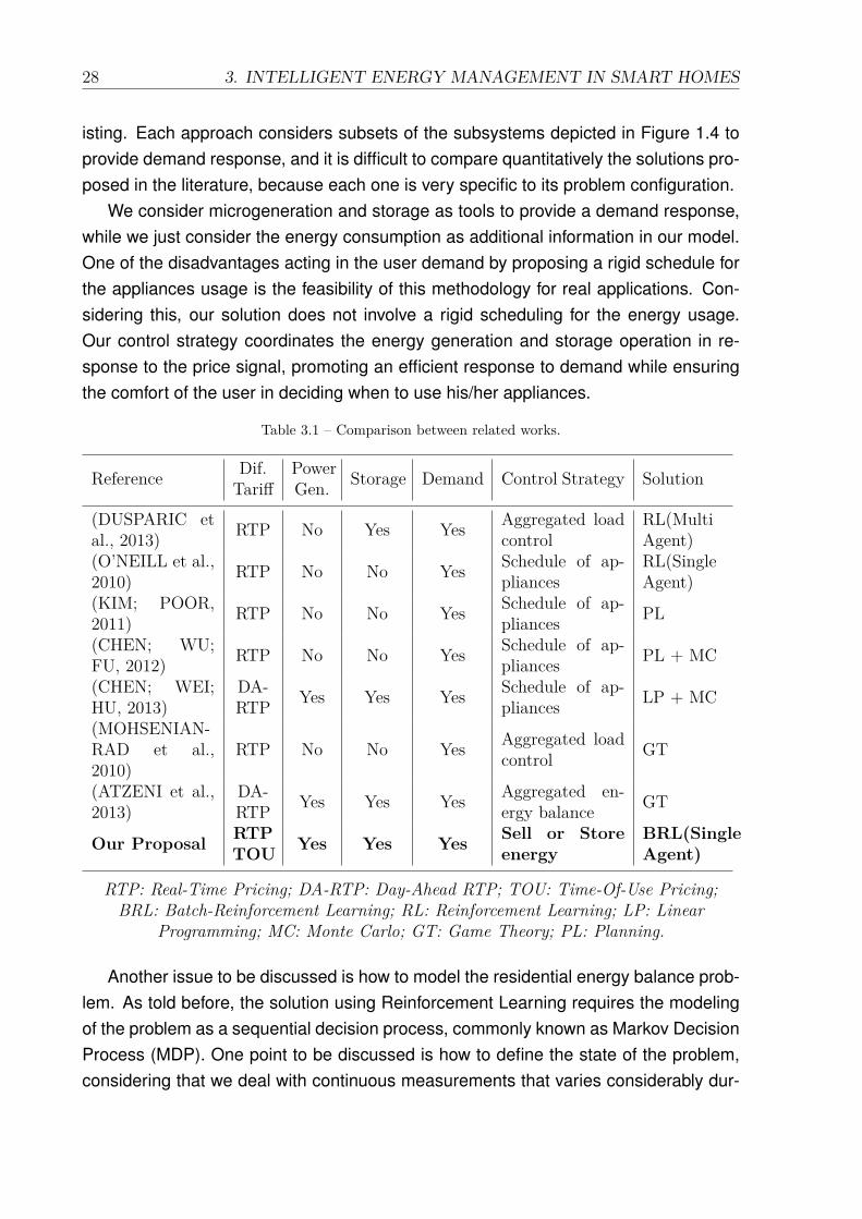
These works considers different ways of dealing with the energy management prob-lem. A comparison between the main points of these works can be viewed in Table 3.1.We can also observe in this table the differences between our proposal and other ex-
28 3. INTELLIGENT ENERGY MANAGEMENT IN SMART HOMES
isting. Each approach considers subsets of the subsystems depicted in Figure 1.4 toprovide demand response, and it is difficult to compare quantitatively the solutions pro-posed in the literature, because each one is very specific to its problem configuration.
We consider microgeneration and storage as tools to provide a demand response,while we just consider the energy consumption as additional information in our model.One of the disadvantages acting in the user demand by proposing a rigid schedule forthe appliances usage is the feasibility of this methodology for real applications. Con-sidering this, our solution does not involve a rigid scheduling for the energy usage.Our control strategy coordinates the energy generation and storage operation in re-sponse to the price signal, promoting an efficient response to demand while ensuringthe comfort of the user in deciding when to use his/her appliances.
Table 3.1 – Comparison between related works.
Reference Dif.Tariff
PowerGen. Storage Demand Control Strategy Solution
(DUSPARIC etal., 2013) RTP No Yes Yes Aggregated load
controlRL(MultiAgent)
(O’NEILL et al.,2010) RTP No No Yes Schedule of ap-
pliancesRL(SingleAgent)
(KIM; POOR,2011) RTP No No Yes Schedule of ap-
pliances PL
(CHEN; WU;FU, 2012) RTP No No Yes Schedule of ap-
pliances PL + MC
(CHEN; WEI;HU, 2013)
DA-RTP Yes Yes Yes Schedule of ap-
pliances LP + MC
(MOHSENIAN-RAD et al.,2010)
RTP No No Yes Aggregated loadcontrol GT
(ATZENI et al.,2013)
DA-RTP Yes Yes Yes Aggregated en-
ergy balance GT
Our Proposal RTPTOU Yes Yes Yes Sell or Store
energyBRL(SingleAgent)
RTP: Real-Time Pricing; DA-RTP: Day-Ahead RTP; TOU: Time-Of-Use Pricing;BRL: Batch-Reinforcement Learning; RL: Reinforcement Learning; LP: Linear
Programming; MC: Monte Carlo; GT: Game Theory; PL: Planning.
Another issue to be discussed is how to model the residential energy balance prob-lem. As told before, the solution using Reinforcement Learning requires the modelingof the problem as a sequential decision process, commonly known as Markov DecisionProcess (MDP). One point to be discussed is how to define the state of the problem,considering that we deal with continuous measurements that varies considerably dur-
3. INTELLIGENT ENERGY MANAGEMENT IN SMART HOMES 29
ing the system operation. Depending on the way these data are treated, the problemstate space can become huge and impossible to deal with.
Considering this, we propose an innovative way to enter price information into themodel as trend indexes, which represents a significant gain if we observe the resultingreduced state space and the amount of information available to be considered in themodel. The discussed works use only the absolute value of the price in their models,not considering the real variation of the energy price (O’NEILL et al., 2010; CHEN; WEI;HU, 2013). We tested our approach in two different pricing models in order to assessits performance in scenarios with different levels of uncertainty in energy prices.
As can be noticed, there are many ways to solve the residential energy manage-ment problem and, at this point, it is difficult to pick a solution as a benchmark. Becauseof the high level of uncertainty involved in the process and the lack of information aboutthe dynamics of the Smart Home subsystems, we propose a learning-based EMS,making the system even adaptive to the variation in the environment dynamics.
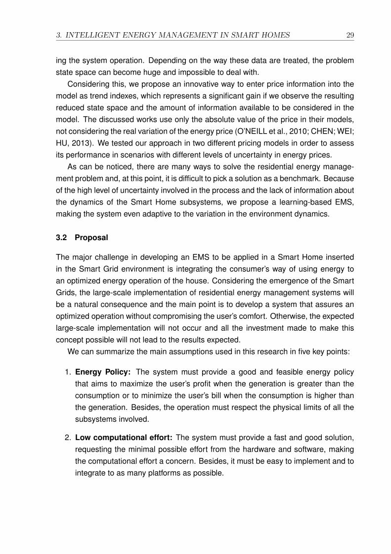
3.2 Proposal
The major challenge in developing an EMS to be applied in a Smart Home insertedin the Smart Grid environment is integrating the consumer’s way of using energy toan optimized energy operation of the house. Considering the emergence of the SmartGrids, the large-scale implementation of residential energy management systems willbe a natural consequence and the main point is to develop a system that assures anoptimized operation without compromising the user’s comfort. Otherwise, the expectedlarge-scale implementation will not occur and all the investment made to make thisconcept possible will not lead to the results expected.
We can summarize the main assumptions used in this research in five key points:
1. Energy Policy: The system must provide a good and feasible energy policythat aims to maximize the user’s profit when the generation is greater than theconsumption or to minimize the user’s bill when the consumption is higher thanthe generation. Besides, the operation must respect the physical limits of all thesubsystems involved.
2. Low computational effort: The system must provide a fast and good solution,requesting the minimal possible effort from the hardware and software, makingthe computational effort a concern. Besides, it must be easy to implement and tointegrate to as many platforms as possible.

30 3. INTELLIGENT ENERGY MANAGEMENT IN SMART HOMES
3. Robustness: The system must be robust enough to deal with the system uncer-tainties.
4. Adaptivity: It is desirable that the system has an adaptive philosophy of oper-ation, i.e., it must be able to follow the changes in the environmental dynamics,keeping the energy operation optimized.
5. User interaction: The interference with the user’s comfort must be minimal. Ifpossible, the user would not be affected by the system operation.
In this work, we present the Reinforcement Learning-based Energy ManagementSystem (RLbEMS). The proposed system considers a centralized architecture of con-trol, i.e., the energy policy is obtained by a single decision-maker that it is responsiblefor acquiring the system information through sensors and for applying the desired ac-tion through actuators. We apply a Free User Policy approach, that considers theenergy supply in an optimized way without the participation of the user. In this case,the user is free to operate the home appliances, generating an energy demand. Ateach instant, the RLbEMS main goal is to operate the auxiliary systems (power gener-ation system and energy storage system) following the pricing signal, in order to meetthe user’s demand in an optimized way.
In this case, the actions performed by the EMS are related to choosing the bestway of using the generated power, considering that it can sell, store or use it. Besides,when the power generation is not enough, the system must also request energy fromthe power grid, following the price signal.
3.2.1 RLbEMS Structure
As can be viewed in Figure 3.4, the System Structure is composed by three indepen-dent stages:
1. Data Acquisition Mode: This step is when the system acquires historical in-formation, HistData =< g(t), d(t), p(t) >, about the energy generation, houseenergy demand and the energy price, as can be viewed in Figure 3.5. Thesedata is stored in a database to be used in the Training Mode.
2. Training Mode: Here the system uses the information stored in the database toobtain an energy selling policy. This mode updates the energy policy periodicallywith a new database.
3. Operation Mode: Once the system has the energy selling policy available, thismode is activated. It corresponds to the system real operation, when it will applythe obtained policy.
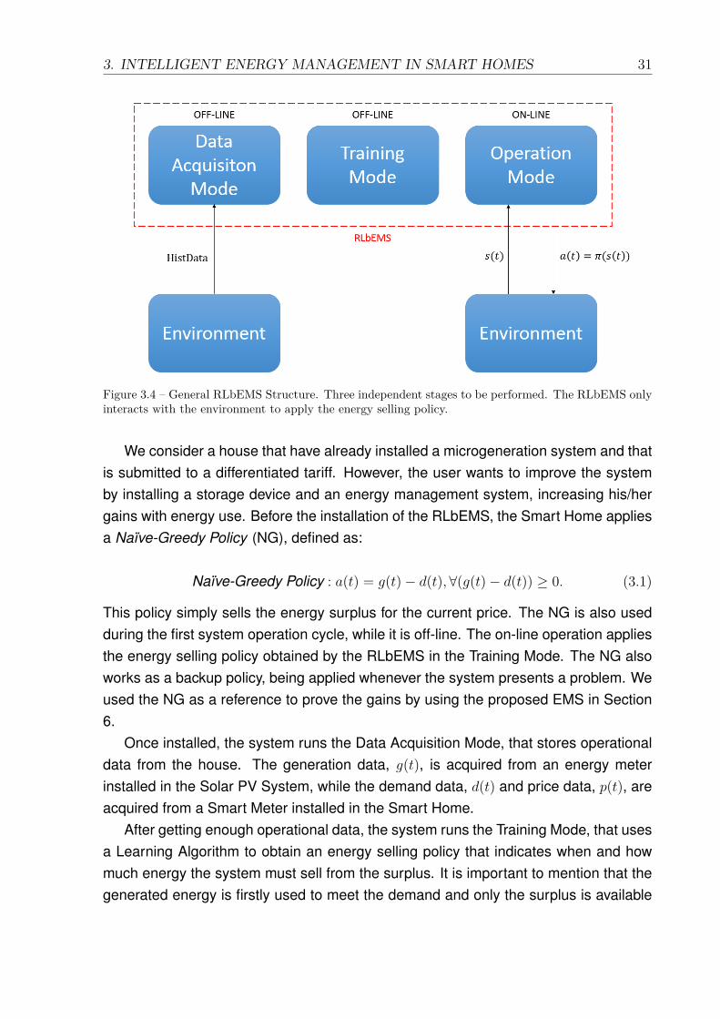
3. INTELLIGENT ENERGY MANAGEMENT IN SMART HOMES 31
Figure 3.4 – General RLbEMS Structure. Three independent stages to be performed. The RLbEMS onlyinteracts with the environment to apply the energy selling policy.
We consider a house that have already installed a microgeneration system and thatis submitted to a differentiated tariff. However, the user wants to improve the systemby installing a storage device and an energy management system, increasing his/hergains with energy use. Before the installation of the RLbEMS, the Smart Home appliesa Naïve-Greedy Policy (NG), defined as:
Naïve-Greedy Policy : a(t) = g(t)− d(t),∀(g(t)− d(t)) ≥ 0. (3.1)
This policy simply sells the energy surplus for the current price. The NG is also usedduring the first system operation cycle, while it is off-line. The on-line operation appliesthe energy selling policy obtained by the RLbEMS in the Training Mode. The NG alsoworks as a backup policy, being applied whenever the system presents a problem. Weused the NG as a reference to prove the gains by using the proposed EMS in Section6.
Once installed, the system runs the Data Acquisition Mode, that stores operationaldata from the house. The generation data, g(t), is acquired from an energy meterinstalled in the Solar PV System, while the demand data, d(t) and price data, p(t), areacquired from a Smart Meter installed in the Smart Home.
After getting enough operational data, the system runs the Training Mode, that usesa Learning Algorithm to obtain an energy selling policy that indicates when and howmuch energy the system must sell from the surplus. It is important to mention that thegenerated energy is firstly used to meet the demand and only the surplus is available
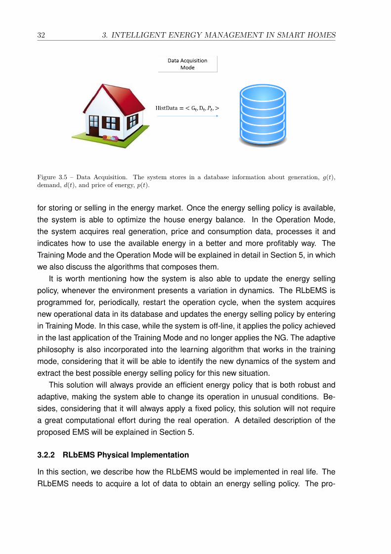
32 3. INTELLIGENT ENERGY MANAGEMENT IN SMART HOMES
Figure 3.5 – Data Acquisition. The system stores in a database information about generation, g(t),demand, d(t), and price of energy, p(t).
for storing or selling in the energy market. Once the energy selling policy is available,the system is able to optimize the house energy balance. In the Operation Mode,the system acquires real generation, price and consumption data, processes it andindicates how to use the available energy in a better and more profitably way. TheTraining Mode and the Operation Mode will be explained in detail in Section 5, in whichwe also discuss the algorithms that composes them.
It is worth mentioning how the system is also able to update the energy sellingpolicy, whenever the environment presents a variation in dynamics. The RLbEMS isprogrammed for, periodically, restart the operation cycle, when the system acquiresnew operational data in its database and updates the energy selling policy by enteringin Training Mode. In this case, while the system is off-line, it applies the policy achievedin the last application of the Training Mode and no longer applies the NG. The adaptivephilosophy is also incorporated into the learning algorithm that works in the trainingmode, considering that it will be able to identify the new dynamics of the system andextract the best possible energy selling policy for this new situation.
This solution will always provide an efficient energy policy that is both robust andadaptive, making the system able to change its operation in unusual conditions. Be-sides, considering that it will always apply a fixed policy, this solution will not requirea great computational effort during the real operation. A detailed description of theproposed EMS will be explained in Section 5.
3.2.2 RLbEMS Physical Implementation
In this section, we describe how the RLbEMS would be implemented in real life. TheRLbEMS needs to acquire a lot of data to obtain an energy selling policy. The pro-
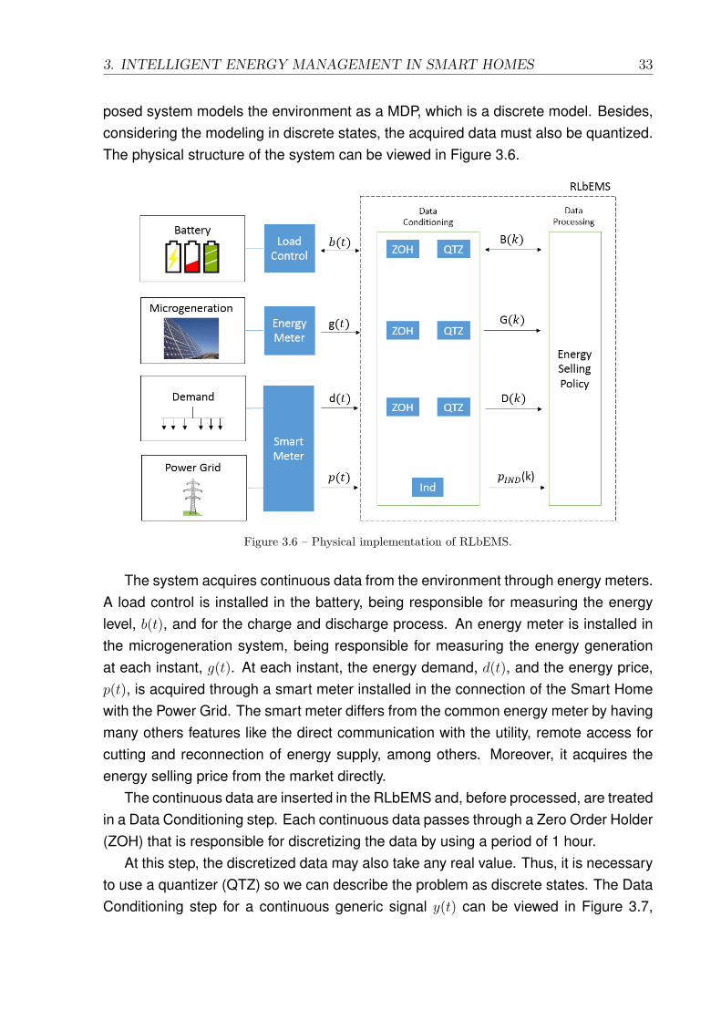
3. INTELLIGENT ENERGY MANAGEMENT IN SMART HOMES 33
posed system models the environment as a MDP, which is a discrete model. Besides,considering the modeling in discrete states, the acquired data must also be quantized.The physical structure of the system can be viewed in Figure 3.6.
Figure 3.6 – Physical implementation of RLbEMS.
The system acquires continuous data from the environment through energy meters.A load control is installed in the battery, being responsible for measuring the energylevel, b(t), and for the charge and discharge process. An energy meter is installed inthe microgeneration system, being responsible for measuring the energy generationat each instant, g(t). At each instant, the energy demand, d(t), and the energy price,p(t), is acquired through a smart meter installed in the connection of the Smart Homewith the Power Grid. The smart meter differs from the common energy meter by havingmany others features like the direct communication with the utility, remote access forcutting and reconnection of energy supply, among others. Moreover, it acquires theenergy selling price from the market directly.
The continuous data are inserted in the RLbEMS and, before processed, are treatedin a Data Conditioning step. Each continuous data passes through a Zero Order Holder(ZOH) that is responsible for discretizing the data by using a period of 1 hour.
At this step, the discretized data may also take any real value. Thus, it is necessaryto use a quantizer (QTZ) so we can describe the problem as discrete states. The DataConditioning step for a continuous generic signal y(t) can be viewed in Figure 3.7,
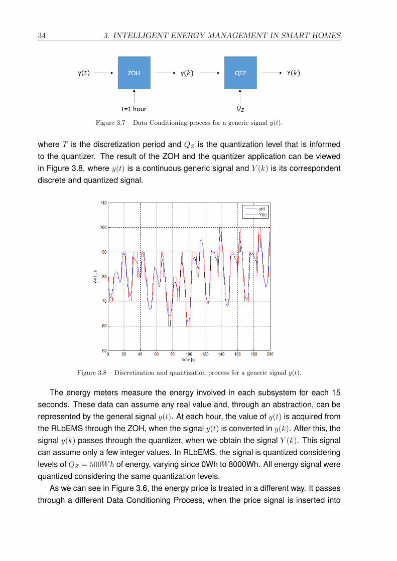
34 3. INTELLIGENT ENERGY MANAGEMENT IN SMART HOMES
Figure 3.7 – Data Conditioning process for a generic signal y(t).
where T is the discretization period and QZ is the quantization level that is informedto the quantizer. The result of the ZOH and the quantizer application can be viewedin Figure 3.8, where y(t) is a continuous generic signal and Y (k) is its correspondentdiscrete and quantized signal.
Figure 3.8 – Discretization and quantization process for a generic signal y(t).
The energy meters measure the energy involved in each subsystem for each 15seconds. These data can assume any real value and, through an abstraction, can berepresented by the general signal y(t). At each hour, the value of y(t) is acquired fromthe RLbEMS through the ZOH, when the signal y(t) is converted in y(k). After this, thesignal y(k) passes through the quantizer, when we obtain the signal Y (k). This signalcan assume only a few integer values. In RLbEMS, the signal is quantized consideringlevels of QZ = 500Wh of energy, varying since 0Wh to 8000Wh. All energy signal werequantized considering the same quantization levels.
As we can see in Figure 3.6, the energy price is treated in a different way. It passesthrough a different Data Conditioning Process, when the price signal is inserted into
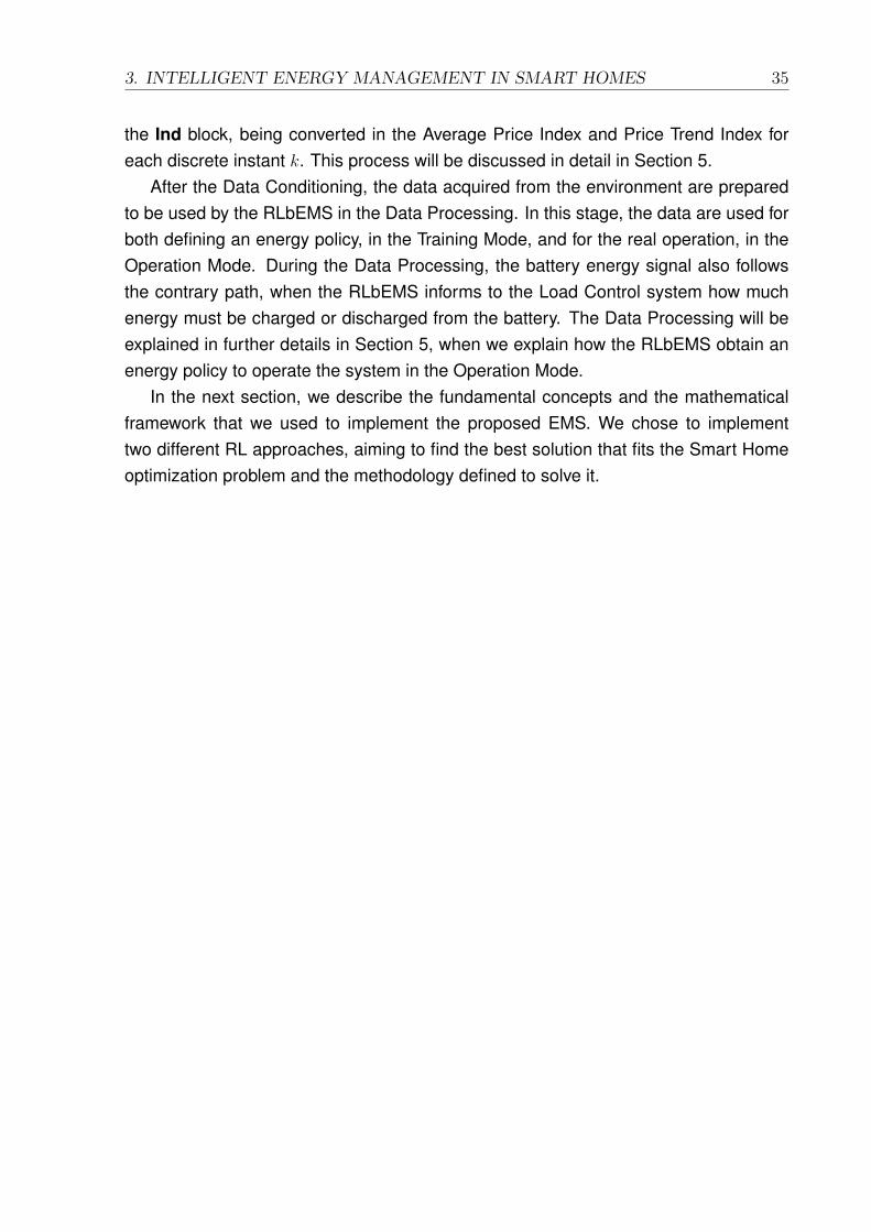
3. INTELLIGENT ENERGY MANAGEMENT IN SMART HOMES 35
the Ind block, being converted in the Average Price Index and Price Trend Index foreach discrete instant k. This process will be discussed in detail in Section 5.
After the Data Conditioning, the data acquired from the environment are preparedto be used by the RLbEMS in the Data Processing. In this stage, the data are used forboth defining an energy policy, in the Training Mode, and for the real operation, in theOperation Mode. During the Data Processing, the battery energy signal also followsthe contrary path, when the RLbEMS informs to the Load Control system how muchenergy must be charged or discharged from the battery. The Data Processing will beexplained in further details in Section 5, when we explain how the RLbEMS obtain anenergy policy to operate the system in the Operation Mode.
In the next section, we describe the fundamental concepts and the mathematicalframework that we used to implement the proposed EMS. We chose to implementtwo different RL approaches, aiming to find the best solution that fits the Smart Homeoptimization problem and the methodology defined to solve it.

36 3. INTELLIGENT ENERGY MANAGEMENT IN SMART HOMES
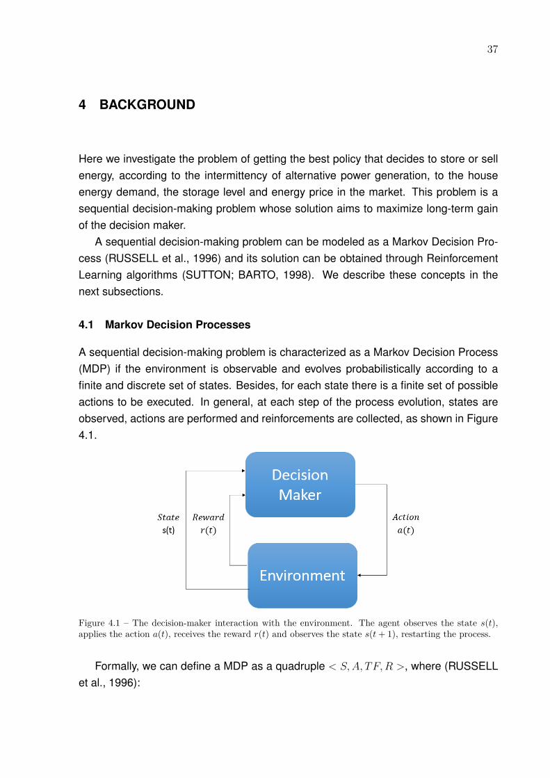
37
4 BACKGROUND
Here we investigate the problem of getting the best policy that decides to store or sellenergy, according to the intermittency of alternative power generation, to the houseenergy demand, the storage level and energy price in the market. This problem is asequential decision-making problem whose solution aims to maximize long-term gainof the decision maker.
A sequential decision-making problem can be modeled as a Markov Decision Pro-cess (RUSSELL et al., 1996) and its solution can be obtained through ReinforcementLearning algorithms (SUTTON; BARTO, 1998). We describe these concepts in thenext subsections.
4.1 Markov Decision Processes
A sequential decision-making problem is characterized as a Markov Decision Process(MDP) if the environment is observable and evolves probabilistically according to afinite and discrete set of states. Besides, for each state there is a finite set of possibleactions to be executed. In general, at each step of the process evolution, states areobserved, actions are performed and reinforcements are collected, as shown in Figure4.1.
Figure 4.1 – The decision-maker interaction with the environment. The agent observes the state s(t),applies the action a(t), receives the reward r(t) and observes the state s(t + 1), restarting the process.
Formally, we can define a MDP as a quadruple < S,A, TF,R >, where (RUSSELLet al., 1996):

38 4. BACKGROUND
• S is a finite set of states, in which s(t) ∈ S for t = 0, ...,∞;
• A is a finite set of possible actions, in which a(t) ∈ A for t = 0, ...,∞;
• TF : S×A×S → [0, 1] is a state transition probability function, which defines thetransition probability from a state s(t) ∈ S to a state s(t + 1) ∈ S when an actiona(t) ∈ A is applied in s(t);
• R : S × A → < is the reward function. So, for each state transition r(t) =R(s(t), a(t));
We define As(s) as the admissible set of actions for a state s ∈ S. So, consideringi ∈ S as the current state, the transition from i ∈ S to j ∈ S in response to theapplication of the action a ∈ As(i) will occur with probability TF (i, a, j) and a rewardR(i, a) will be received.
Thus, on each step, the decision-maker observes the current state s(t) of the envi-ronment and must choose the best action to perform. After executing the action a(t),it receives a reward r(t) and the environment evolves for the next state s(t + 1), whichwill be observed in the next step. The probability of transition from a current state toanother future state depends only on the current state and the action taken at this in-stant. This is known as the Markov Property (SUTTON; BARTO, 1998). The reward isa measure of the value of the applied action, considering the goals of the optimizationproblem.
Solving a MDP means finding a policy π that specifies which action must be exe-cuted in each state, considering the maximization of the discounted cumulative rewardsduring an infinitive time horizon.
The total number of steps in which the decision maker must achieve its goals iscalled Horizon. A MDP can be defined as Finite Horizon, when there is a specific andfixed number of steps, or Infinite Horizon, when the number of steps is consideredinfinite. Also, there is a Undetermined Horizon, when the agent runs until it achievesthe predefined goal. In general, the policy that solves a finite horizon MDP is moreaggressive than the policy obtained to solve the same MDP if we consider an infinitehorizon, because, in the first case, the decision maker has a few number of steps tomaximize its goals.
The modeling as finite or infinite horizon has to do with the system characteristics.The problem studied can be treated in both ways, considering that the decision makershould maximize the accumulated rewards in a specific period as a month, for example,or over a long period considered infinite. In this work, we chose to model the system asan infinite horizon MDP, because the system has slow dynamics and the return of the
4. BACKGROUND 39
investment made is long-term. The policy obtained in this case is a stationary Marko-vian policy, i.e., it does not consider the time while choosing actions to be performed.The decision maker only considers the current state to choose actions.
Considering a policy π and an initial state s0, we can define Value Function as theexpected cumulative reward obtained from the application of policy π until the end ofthe time horizon. Mathematically, we have:
V π(s) = E[∞∑t=0
γtr(t)|π, s0 = s],∀sεS, (4.1)
where γ, 0 < γ ≤ 1, is a constant called discount factor, that ponders the rewardreceived during time, and r(t) is the reward received in each step t. The optimal policyπ∗ is the one that maximizes the value function for each state, which corresponds tothe optimal value function V ∗. Considering real problems, solving a MDP is related tofinding the policy that is the best approximation of the optimal policy.
There are many ways of solving a MDP, depending on the problem studied andthe available information about the system. Considering real problems, sometimes it isdifficult to obtain a complete system model as specified above. In these cases, learningalgorithms are needed, because the agent must decide the best action to perform ineach state while learning about the state probability function or the reward function thatis sometimes unknown. One way to solve this problem is applying a ReinforcementLearning algorithm (SUTTON; BARTO, 1998), which is based on acquiring knowledgethrough interactions with the environment.
The modeling of the problem as a classical MDP considers two sets of discretestates and actions, which differs from many real world control problems that requireactions of a continuous nature, in response to continuous state measurements. Onthe other hand, the efficiency of the learning process it is known to decrease while weincrease the number of possible states and actions. In the literature, there are manyways of generalizing the discrete policy obtained for the application in real problems.Artificial Neural Networks, CMAC (Cerebellar Model Articulation Controller) and otherapproaches can be used to generalize the policy obtained. In other situations, a goodsolution is to directly model and to solve the problem in a continuous way using acontinuous formulation for the MDP. A natural evolution of the system proposed mustinclude such generalization, but this is not a specific goal of this research for a while.
4.2 Reinforcement Learning and Q-Learning Algorithm
Learning techniques are characterized by the modification of the decision-making mech-anism aiming to improve the performance of the control system. Those techniques are
40 4. BACKGROUND
often used in problems in which the environments explored are unknown. Reinforce-ment learning (RL) is an experimentation-based learning technique, i.e., the knowl-edge about the environment is acquired from the responses to the actions taken ineach state. Thus, the main goal is to find out which actions should be applied in eachstate of the system to maximize the expected long-term reward (or reinforcement) whilelearning about the environment.
RL is one way of solving a MDP in problems for which the agent has little informationabout the controlled system (SUTTON; BARTO, 1998). Q-Learning (WATKINS, 1989)was the first RL algorithm obtained to perform an experimentation-based learning, andensures that an optimal policy is found if the environment can be modeled as a MDPand if the agent explores the environment in a way that never completely ignores anystate or action.
The Q-Learning algorithm is based on the Value-Action Function, defined as:
Q(s(t), a(t)) = R(s(t), a(t)) + γ.V ∗(s(t+ 1)), (4.2)
where Q : S ×A→ < is a real function that expresses the expected value of the futurerewards, Q(.), when an action a(t) is applied in a state s(t).
The core of the algorithm is based on a recursive equation that is responsible for theestimation of the final value of Q(s, a) for each pair state-action. The value of Q(s, a) isupdated at each step considering the following equation:
QNew(s(t), a(t))← [r(t) + γmaxa
Q(s(t+ 1), a)], (4.3)
Q(s(t), a(t))← (1− α)Q(s(t), a(t)) + αQNew(s(t), a(t)), (4.4)
where s(t) and a(t) are the observed state and the applied action on the step t, re-spectively; r(t) is the received reward after applying a(t) in s(t); α is a constant valuecalled learning rate that varies from 0 to 1 and that reflects how the agent will ponderthe new and the old information of Q(s(t), a(t)); and γ is the discount factor that reflectsthe importance given to future rewards.
The main goal of the Q-Learning algorithm is to estimate the values of Q(s, a) ex-haustively until its values stabilize and converge to the optimal value. In the algorithm,QS×A is defined as a matrix with the number of rows and columns equal to the numberof states, |S|, and actions, |A|, respectively. Q-Learning is described in Algorithm 1.
After all, the optimal policy is obtained by choosing in matrix QS×A which actionsmaximize the final value-action for each state. This procedure can be mathematicallydefined as:

4. BACKGROUND 41
Algorithm 1 Q-Learning Algorithm. Initialize the table entry QS×A to zero.Observe the current state s(t)while TRUE do
Select an action a(t) and execute itReceive immediate reward r(t)Observe the new state s(t+ 1)Update the table entry for Q(s(t), a(t)) (Eq. 4.4)s(t)← s(t+ 1)
π∗(s) = arg maxaεA
Q(s, a),∀sεS. (4.5)
Therefore, for each state there is an action that, if applied, will maximize the rewardsreceived in the horizon of actuation considered.
4.3 Batch-Reinforcement Learning
The problem studied in this research is composed of a set of different subsystems,each one with its specific operation characteristics and level of uncertainty. As will bediscussed in Section 6, the solution using classical reinforcement learning algorithmsneeds too much computational time. Besides, considering the usual small set of his-torical data available, the algorithm does not reaches the convergence to the optimalpolicy.
The application of model-free on-line learning methods such as the Q-learning al-gorithm (WATKINS, 1989) is only feasible when we deal with problems described by asmall discrete state space, which avoids the curse of dimensionality that characterizesmethods based on dynamic programming (DP) (BELLMAN, 1957). However, whenapplied in realistic systems and/or continuous systems, this results in a large state ofspace, making its solution almost unfeasible.
Batch Reinforcement Learning (Batch-RL) is a subfield of dynamic programmingwhose main purpose is the solution of the problems mentioned due to its efficient useof collected data and to the stability of the learning process. Moreover, it can providea better solution for a MDP composed of a great number of states faster than classicalreinforcement learning algorithms.
In this section, we describe the Batch-RL problem and discuss the main character-istics that make this technique a better solution for the problem proposed.
42 4. BACKGROUND
4.3.1 The Batch-Reinforcement Learning Problem
The concept of batch reinforcement learning is used to describe a reinforcement learn-ing setting, where the complete amount of learning experience is fixed and given a pri-ori (ERNST et al., 2005a). One of the first to use this structure was Ormoneit e Glynn(2002), which implemented the Q-Function determination problem as a sequence ofkernel-based regression problems. Considering the learning experience as a set oftransitions samples from the system, the learning mechanism involves finding the bestsolution out of this given batch of samples. The major benefit of this approach is theway they use the amount of available data and get the best of it, even considering afixed set of samples, and the stability of the learning process.
The convergence in a fraction of time used by pure on-line methods and the learningmechanism using a predefined set of given samples are crucial for implementing thistechnique in real problems, because we usually need a good solution in a faster wayand with the lowest possible process interaction.
As stated before, the reinforcement learning problem is characterized by the learn-ing from the interaction mechanism, i.e., the agent must find an actuation policy thatmaximizes the sum of expected rewards only through its interaction with the environ-ment. In a different way, in the Batch-RL problem, the agent does not interact directlywith the environment. Instead of observing a state s, applying an action a and updat-ing its policy in response to the reinforcement obtained at each instant of operation,the agent receives a set of data, F , that contains n transitions (s(t), a(t), r(t), s(t + 1))sampled from the environment:
F = {(s(t), a(t), r(t), s(t+ 1))|t = 1, ..., n}. (4.6)
In this approach, the exploration, learning and application mechanisms are inde-pendent of each other. As illustrated in Figure 4.2, each step has its own distinctmechanism of operation. Thus:
• Exploration: Collecting system transitions with an arbitrary sampling strategy.
• Learning: Application of Batch-RL algorithm in order to learn the best possiblepolicy from the given set of transitions.
• Execution: Application of the policy obtained from the controlled process.
As can be verified, the exploration is a separate part of the learning process, whichdiffers from the on-line learning mechanism and avoids the dilemma of exploiting orexploring. Besides, the execution is also separate, i.e., the policy remains fixed and isnot improved further.
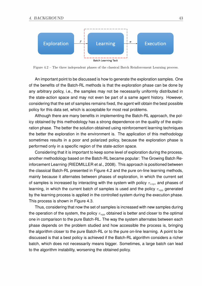
4. BACKGROUND 43
Figure 4.2 – The three independent phases of the classical Batch Reinforcement Learning process.
An important point to be discussed is how to generate the exploration samples. Oneof the benefits of the Batch-RL methods is that the exploration phase can be done byany arbitrary policy, i.e., the samples may not be necessarily uniformly distributed inthe state-action space and may not even be part of a same agent history. However,considering that the set of samples remains fixed, the agent will obtain the best possiblepolicy for this data set, which is acceptable for most real problems.
Although there are many benefits in implementing the Batch-RL approach, the pol-icy obtained by this methodology has a strong dependence on the quality of the explo-ration phase. The better the solution obtained using reinforcement learning techniquesthe better the exploration in the environment is. The application of this methodologysometimes results in a poor and polarized policy, because the exploration phase isperformed only in a specific region of the state-action space.
Considering that it is important to keep some level of exploration during the process,another methodology based on the Batch-RL became popular: The Growing Batch Re-inforcement Learning (RIEDMILLER et al., 2008). This approach is positioned betweenthe classical Batch-RL presented in Figure 4.2 and the pure on-line learning methods,mainly because it alternates between phases of exploration, in which the current setof samples is increased by interacting with the system with policy πexp, and phases oflearning, in which the current batch of samples is used and the policy πapp generatedby the learning process is applied in the controlled system during the execution phase.This process is shown in Figure 4.3.
Thus, considering that now the set of samples is increased with new samples duringthe operation of the system, the policy πapp obtained is better and closer to the optimalone in comparison to the pure Batch-RL. The way the system alternates between eachphase depends on the problem studied and how accessible the process is, bringingthe algorithm closer to the pure Batch-RL or to the pure on-line learning. A point to bediscussed is that a best policy is achieved if the Batch-RL algorithm considers a richerbatch, which does not necessarily means bigger. Sometimes, a large batch can leadto the algorithm instability, worsening the obtained policy.
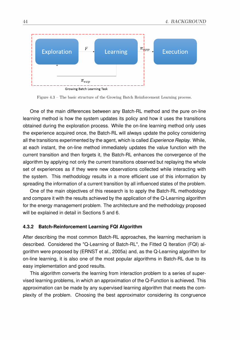
44 4. BACKGROUND
Figure 4.3 – The basic structure of the Growing Batch Reinforcement Learning process.
One of the main differences between any Batch-RL method and the pure on-linelearning method is how the system updates its policy and how it uses the transitionsobtained during the exploration process. While the on-line learning method only usesthe experience acquired once, the Batch-RL will always update the policy consideringall the transitions experimented by the agent, which is called Experience Replay. While,at each instant, the on-line method immediately updates the value function with thecurrent transition and then forgets it, the Batch-RL enhances the convergence of thealgorithm by applying not only the current transitions observed but replaying the wholeset of experiences as if they were new observations collected while interacting withthe system. This methodology results in a more efficient use of this information byspreading the information of a current transition by all influenced states of the problem.
One of the main objectives of this research is to apply the Batch-RL methodologyand compare it with the results achieved by the application of the Q-Learning algorithmfor the energy management problem. The architecture and the methodology proposedwill be explained in detail in Sections 5 and 6.
4.3.2 Batch-Reinforcement Learning FQI Algorithm
After describing the most common Batch-RL approaches, the learning mechanism isdescribed. Considered the "Q-Learning of Batch-RL", the Fitted Q Iteration (FQI) al-gorithm were proposed by (ERNST et al., 2005a) and, as the Q-Learning algorithm foron-line learning, it is also one of the most popular algorithms in Batch-RL due to itseasy implementation and good results.
This algorithm converts the learning from interaction problem to a series of super-vised learning problems, in which an approximation of the Q-Function is achieved. Thisapproximation can be made by any supervised learning algorithm that meets the com-plexity of the problem. Choosing the best approximator considering its congruence

4. BACKGROUND 45
with the studied problem is critical to ensure the approximation quality and, therefore,the obtained policy.
The algorithm can be summarized in two main steps. Considering a fixed set F ={(s(t), a(t), r(t), s(t+ 1))|t = 1, ..., n} of n transitions and an initial Q-value, q̄0, such thatQ̄0(S,A) = q̄0, ∀(s, a), s ∈ S, a ∈ A. Hence:
• Step 1: Consider TSi+1 a training set defined as (s, a; q̄i+1s,a ), in which (s, a) are
the inputs and q̄i+1s,a are the targets of a Supervised Learning problem. Such that,
for each transition (s(t), a(t), r(t), s(t+ 1)):
q̄i+1s,a = r + γ ×max
a∈AQ̄i(s(t+ 1), a), (4.7)
where q̄i+1s,a is the updated value and Q̄i is the approximation of the Q-value. Then,
the new training set is the last one united to the updated values of q̄i+1s,a :
TSi+1 ← TSi+1 ⋃{(s, a; q̄i+1
s,a )} (4.8)
• Step 2: Use supervised learning to train a function approximator on the patternset TSi+1.
In the end, the resulting function, Q̄i+1, is an approximation of the Q-function Qi+1
after i + 1 steps of dynamic programming. Thus, considering that FQI represents theQ-function explicitly, we can use a greedy policy in FQI such that:
πi(s) = arg maxaεA
Q̄i(s, a),∀s ∈ S. (4.9)
The complete algorithm can be viewed in Algorithm 2.This procedure can be implemented for either a classical Batch-RL or a Growing
Batch-RL. For the classical Batch-RL, the procedure is performed only once consid-ering that the set of samples is fixed; for the Growing Batch-RL, this procedure isrepeated after the exploration step in the learning process.

46 4. BACKGROUND
Algorithm 2 Fitted Q-Iteration Algorithm. Define Q̄0(S,A) = q̄0, ∀(s, a), s ∈ S, a ∈ A.. Define H as the Horizon to be performed;. Load F = {(s(t), a(t), r(t), s(t+ 1))|t = 1, ..., n};. Define TSh ← (s, a; q̄hs,a) as an initial Training Set.while h ≤ H do
for ∀sample ∈ F doq̄h+1s,a = r + γ ×maxa∈A Q̄h(s(t+ 1), a);TSh ← TSh
⋃{(s, a; q̄hs,a)};%%Supervised LearningUse supervised learning to train a function approximator Q̄h(s, a) on the pattern
set TShh← h+ 1;
%% Obtaining Policy %%for ∀sεS do
πh(s) = arg maxaεA Q̄h(s, a),∀s ∈ S;
4.4 A Benchmark Problem
A Benchmark Problem was defined to apply and study the algorithms described before.The main objective is to implement both Q-Learning and FQI algorithms in a simpleproblem, in order to evaluate the algorithms functionalities. Besides, in FQI, we trieddifferent Supervised Learning algorithms, defining also the one that will be used in theEMS implementation.
Figure 4.4 – Benchmark Problem: Gridworld (SUTTON; BARTO, 1998).
We chose to implement a simple problem called Gridworld Problem that can beviewed in Figure 4.4. The main objective of the problem is to achieve one of shadedcells in the corners. Each state of the environment is represented by the cells of thegrid and, at each cell, the agent can apply four possible actions: north, east, south and
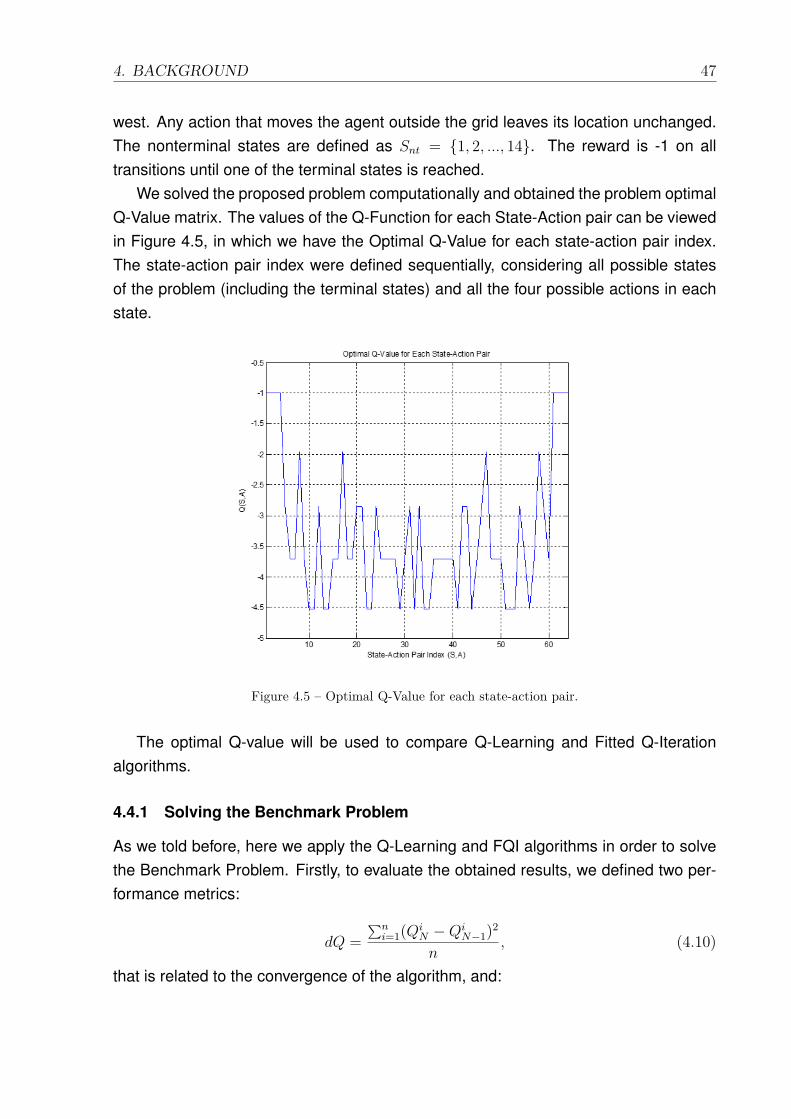
4. BACKGROUND 47
west. Any action that moves the agent outside the grid leaves its location unchanged.The nonterminal states are defined as Snt = {1, 2, ..., 14}. The reward is -1 on alltransitions until one of the terminal states is reached.
We solved the proposed problem computationally and obtained the problem optimalQ-Value matrix. The values of the Q-Function for each State-Action pair can be viewedin Figure 4.5, in which we have the Optimal Q-Value for each state-action pair index.The state-action pair index were defined sequentially, considering all possible statesof the problem (including the terminal states) and all the four possible actions in eachstate.
Figure 4.5 – Optimal Q-Value for each state-action pair.
The optimal Q-value will be used to compare Q-Learning and Fitted Q-Iterationalgorithms.
4.4.1 Solving the Benchmark Problem
As we told before, here we apply the Q-Learning and FQI algorithms in order to solvethe Benchmark Problem. Firstly, to evaluate the obtained results, we defined two per-formance metrics:
dQ =∑ni=1(Qi
N −QiN−1)2
n, (4.10)
that is related to the convergence of the algorithm, and:
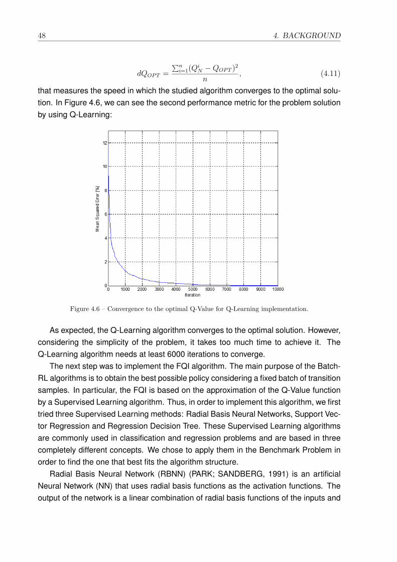
48 4. BACKGROUND
dQOPT =∑ni=1(Qi
N −QOPT )2
n, (4.11)
that measures the speed in which the studied algorithm converges to the optimal solu-tion. In Figure 4.6, we can see the second performance metric for the problem solutionby using Q-Learning:
Figure 4.6 – Convergence to the optimal Q-Value for Q-Learning implementation.
As expected, the Q-Learning algorithm converges to the optimal solution. However,considering the simplicity of the problem, it takes too much time to achieve it. TheQ-Learning algorithm needs at least 6000 iterations to converge.
The next step was to implement the FQI algorithm. The main purpose of the Batch-RL algorithms is to obtain the best possible policy considering a fixed batch of transitionsamples. In particular, the FQI is based on the approximation of the Q-Value functionby a Supervised Learning algorithm. Thus, in order to implement this algorithm, we firsttried three Supervised Learning methods: Radial Basis Neural Networks, Support Vec-tor Regression and Regression Decision Tree. These Supervised Learning algorithmsare commonly used in classification and regression problems and are based in threecompletely different concepts. We chose to apply them in the Benchmark Problem inorder to find the one that best fits the algorithm structure.
Radial Basis Neural Network (RBNN) (PARK; SANDBERG, 1991) is an artificialNeural Network (NN) that uses radial basis functions as the activation functions. Theoutput of the network is a linear combination of radial basis functions of the inputs and
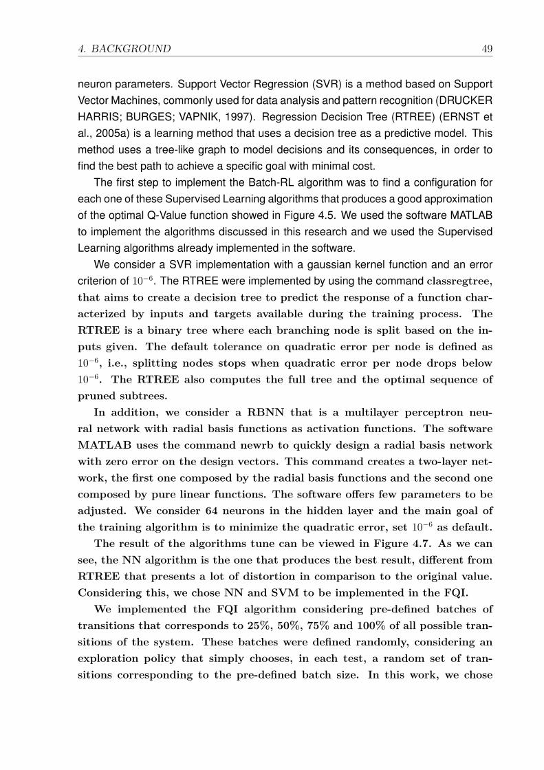
4. BACKGROUND 49
neuron parameters. Support Vector Regression (SVR) is a method based on SupportVector Machines, commonly used for data analysis and pattern recognition (DRUCKERHARRIS; BURGES; VAPNIK, 1997). Regression Decision Tree (RTREE) (ERNST etal., 2005a) is a learning method that uses a decision tree as a predictive model. Thismethod uses a tree-like graph to model decisions and its consequences, in order tofind the best path to achieve a specific goal with minimal cost.
The first step to implement the Batch-RL algorithm was to find a configuration foreach one of these Supervised Learning algorithms that produces a good approximationof the optimal Q-Value function showed in Figure 4.5. We used the software MATLABto implement the algorithms discussed in this research and we used the SupervisedLearning algorithms already implemented in the software.
We consider a SVR implementation with a gaussian kernel function and an errorcriterion of 10−6. The RTREE were implemented by using the command classregtree,that aims to create a decision tree to predict the response of a function char-acterized by inputs and targets available during the training process. TheRTREE is a binary tree where each branching node is split based on the in-puts given. The default tolerance on quadratic error per node is defined as10−6, i.e., splitting nodes stops when quadratic error per node drops below10−6. The RTREE also computes the full tree and the optimal sequence ofpruned subtrees.
In addition, we consider a RBNN that is a multilayer perceptron neu-ral network with radial basis functions as activation functions. The softwareMATLAB uses the command newrb to quickly design a radial basis networkwith zero error on the design vectors. This command creates a two-layer net-work, the first one composed by the radial basis functions and the second onecomposed by pure linear functions. The software offers few parameters to beadjusted. We consider 64 neurons in the hidden layer and the main goal ofthe training algorithm is to minimize the quadratic error, set 10−6 as default.
The result of the algorithms tune can be viewed in Figure 4.7. As we cansee, the NN algorithm is the one that produces the best result, different fromRTREE that presents a lot of distortion in comparison to the original value.Considering this, we chose NN and SVM to be implemented in the FQI.
We implemented the FQI algorithm considering pre-defined batches oftransitions that corresponds to 25%, 50%, 75% and 100% of all possible tran-sitions of the system. These batches were defined randomly, considering anexploration policy that simply chooses, in each test, a random set of tran-sitions corresponding to the pre-defined batch size. In this work, we chose
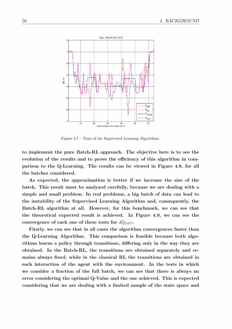
50 4. BACKGROUND
Figure 4.7 – Tune of the Supervised Learning Algorithms.
to implement the pure Batch-RL approach. The objective here is to see theevolution of the results and to prove the efficiency of this algorithm in com-parison to the Q-Learning. The results can be viewed in Figure 4.8, for allthe batches considered.
As expected, the approximation is better if we increase the size of thebatch. This result must be analyzed carefully, because we are dealing with asimple and small problem. In real problems, a big batch of data can lead tothe instability of the Supervised Learning Algorithm and, consequently, theBatch-RL algorithm at all. However, for this benchmark, we can see thatthe theoretical expected result is achieved. In Figure 4.9, we can see theconvergence of each one of these tests for dQOPT .
Firstly, we can see that in all cases the algorithm convergences faster thanthe Q-Learning Algorithm. This comparison is feasible because both algo-rithms learns a policy through transitions, differing only in the way they areobtained. In the Batch-RL, the transitions are obtained separately and re-mains always fixed, while in the classical RL the transitions are obtained ineach interaction of the agent with the environment. In the tests in whichwe consider a fraction of the full batch, we can see that there is always anerror considering the optimal Q-Value and the one achieved. This is expectedconsidering that we are dealing with a limited sample of the state space and
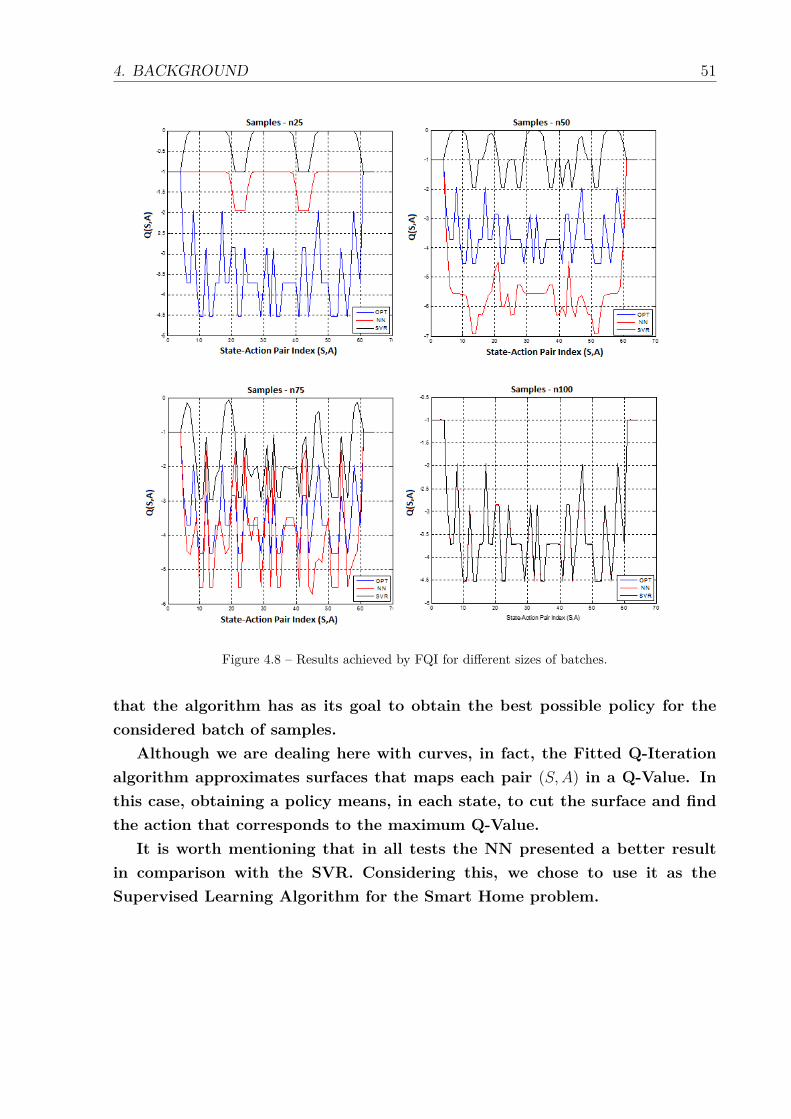
4. BACKGROUND 51
Figure 4.8 – Results achieved by FQI for different sizes of batches.
that the algorithm has as its goal to obtain the best possible policy for theconsidered batch of samples.
Although we are dealing here with curves, in fact, the Fitted Q-Iterationalgorithm approximates surfaces that maps each pair (S,A) in a Q-Value. Inthis case, obtaining a policy means, in each state, to cut the surface and findthe action that corresponds to the maximum Q-Value.
It is worth mentioning that in all tests the NN presented a better resultin comparison with the SVR. Considering this, we chose to use it as theSupervised Learning Algorithm for the Smart Home problem.
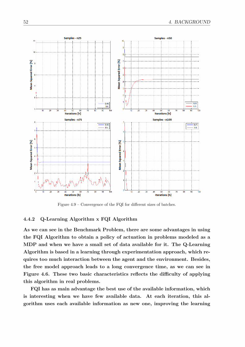
52 4. BACKGROUND
Figure 4.9 – Convergence of the FQI for different sizes of batches.
4.4.2 Q-Learning Algorithm x FQI Algorithm
As we can see in the Benchmark Problem, there are some advantages in usingthe FQI Algorithm to obtain a policy of actuation in problems modeled as aMDP and when we have a small set of data available for it. The Q-LearningAlgorithm is based in a learning through experimentation approach, which re-quires too much interaction between the agent and the environment. Besides,the free model approach leads to a long convergence time, as we can see inFigure 4.6. These two basic characteristics reflects the difficulty of applyingthis algorithm in real problems.
FQI has as main advantage the best use of the available information, whichis interesting when we have few available data. At each iteration, this al-gorithm uses each available information as new one, improving the learning

4. BACKGROUND 53
process. Moreover, the fitting capacity allows the algorithm to estimate val-ues for the Q-function even when there is no information about a specificstate-action pair. This characteristic will be important for the Smart Homeproblem.
However, the use of the FQI must be done carefully and under specificconditions. As we work with a fixed batch of transition samples acquired apriori, the obtained policy directly depends on how the batch of samples wasacquired. A good batch not necessarily means the bigger one, but the onethat was achieved considering a good sampling rule. As the algorithm workswith an approximation of the Q-Function, the policy obtained is a suboptimalpolicy, the best possible suboptimal policy for the available batch. In caseswhen we have few data available, it is expected that the result will be betterthan the Q-Learning algorithm.

54 4. BACKGROUND
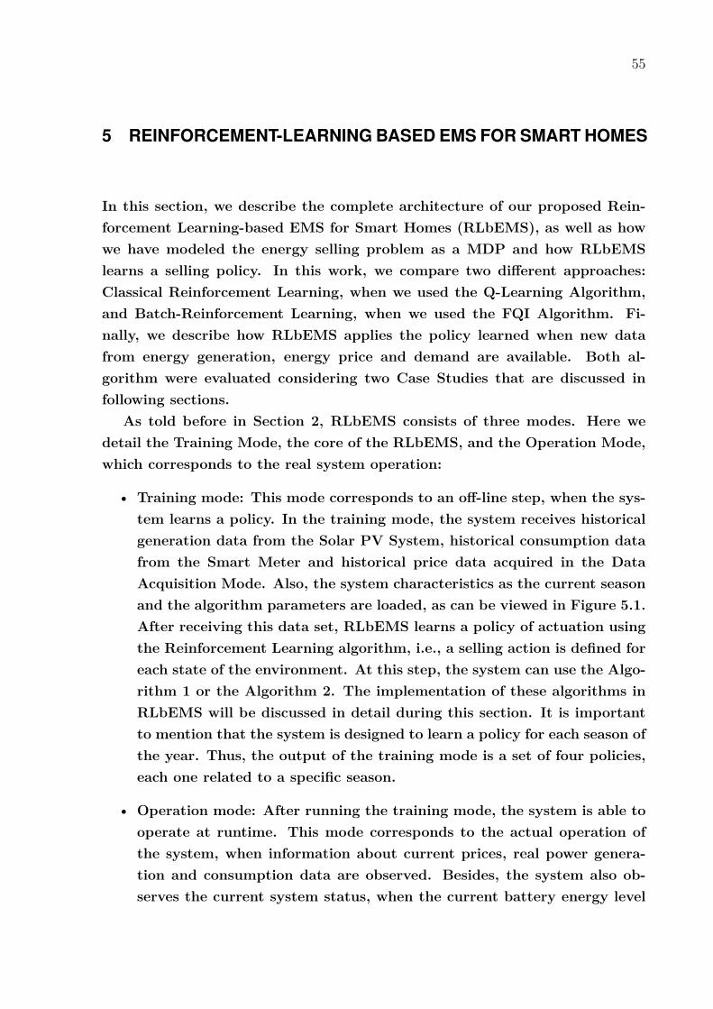
55
5 REINFORCEMENT-LEARNING BASED EMS FOR SMART HOMES
In this section, we describe the complete architecture of our proposed Rein-forcement Learning-based EMS for Smart Homes (RLbEMS), as well as howwe have modeled the energy selling problem as a MDP and how RLbEMSlearns a selling policy. In this work, we compare two different approaches:Classical Reinforcement Learning, when we used the Q-Learning Algorithm,and Batch-Reinforcement Learning, when we used the FQI Algorithm. Fi-nally, we describe how RLbEMS applies the policy learned when new datafrom energy generation, energy price and demand are available. Both al-gorithm were evaluated considering two Case Studies that are discussed infollowing sections.
As told before in Section 2, RLbEMS consists of three modes. Here wedetail the Training Mode, the core of the RLbEMS, and the Operation Mode,which corresponds to the real system operation:
• Training mode: This mode corresponds to an off-line step, when the sys-tem learns a policy. In the training mode, the system receives historicalgeneration data from the Solar PV System, historical consumption datafrom the Smart Meter and historical price data acquired in the DataAcquisition Mode. Also, the system characteristics as the current seasonand the algorithm parameters are loaded, as can be viewed in Figure 5.1.After receiving this data set, RLbEMS learns a policy of actuation usingthe Reinforcement Learning algorithm, i.e., a selling action is defined foreach state of the environment. At this step, the system can use the Algo-rithm 1 or the Algorithm 2. The implementation of these algorithms inRLbEMS will be discussed in detail during this section. It is importantto mention that the system is designed to learn a policy for each season ofthe year. Thus, the output of the training mode is a set of four policies,each one related to a specific season.
• Operation mode: After running the training mode, the system is able tooperate at runtime. This mode corresponds to the actual operation ofthe system, when information about current prices, real power genera-tion and consumption data are observed. Besides, the system also ob-serves the current system status, when the current battery energy level
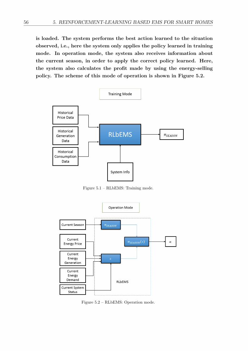
56 5. REINFORCEMENT-LEARNING BASED EMS FOR SMART HOMES
is loaded. The system performs the best action learned to the situationobserved, i.e., here the system only applies the policy learned in trainingmode. In operation mode, the system also receives information aboutthe current season, in order to apply the correct policy learned. Here,the system also calculates the profit made by using the energy-sellingpolicy. The scheme of this mode of operation is shown in Figure 5.2.
Figure 5.1 – RLbEMS: Training mode.
Figure 5.2 – RLbEMS: Operation mode.
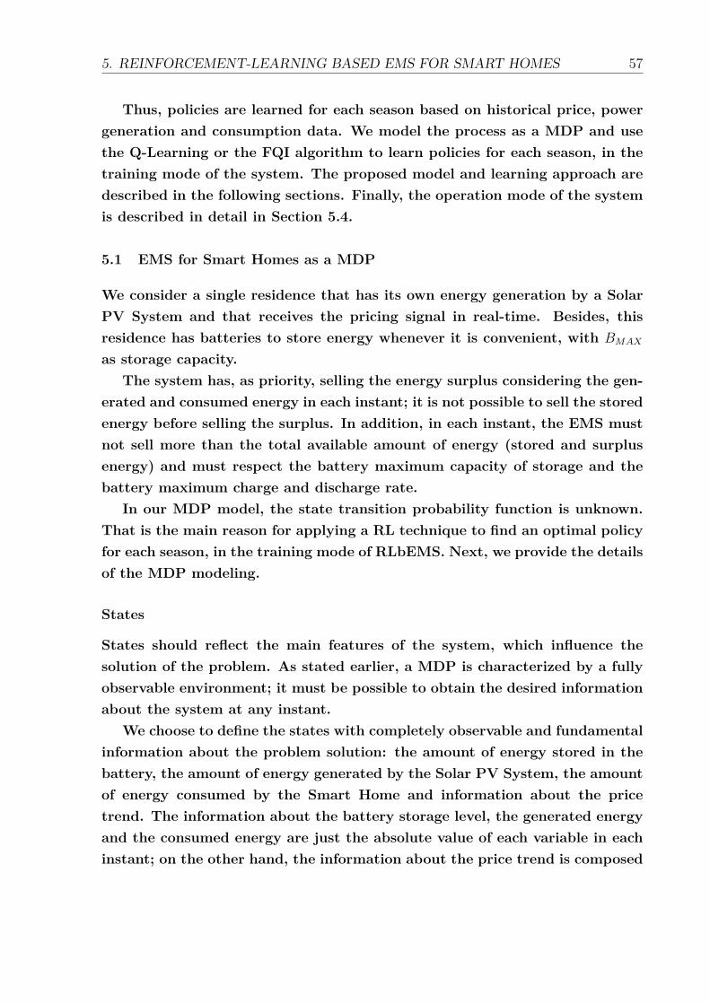
5. REINFORCEMENT-LEARNING BASED EMS FOR SMART HOMES 57
Thus, policies are learned for each season based on historical price, powergeneration and consumption data. We model the process as a MDP and usethe Q-Learning or the FQI algorithm to learn policies for each season, in thetraining mode of the system. The proposed model and learning approach aredescribed in the following sections. Finally, the operation mode of the systemis described in detail in Section 5.4.
5.1 EMS for Smart Homes as a MDP
We consider a single residence that has its own energy generation by a SolarPV System and that receives the pricing signal in real-time. Besides, thisresidence has batteries to store energy whenever it is convenient, with BMAX
as storage capacity.The system has, as priority, selling the energy surplus considering the gen-
erated and consumed energy in each instant; it is not possible to sell the storedenergy before selling the surplus. In addition, in each instant, the EMS mustnot sell more than the total available amount of energy (stored and surplusenergy) and must respect the battery maximum capacity of storage and thebattery maximum charge and discharge rate.
In our MDP model, the state transition probability function is unknown.That is the main reason for applying a RL technique to find an optimal policyfor each season, in the training mode of RLbEMS. Next, we provide the detailsof the MDP modeling.
States
States should reflect the main features of the system, which influence thesolution of the problem. As stated earlier, a MDP is characterized by a fullyobservable environment; it must be possible to obtain the desired informationabout the system at any instant.
We choose to define the states with completely observable and fundamentalinformation about the problem solution: the amount of energy stored in thebattery, the amount of energy generated by the Solar PV System, the amountof energy consumed by the Smart Home and information about the pricetrend. The information about the battery storage level, the generated energyand the consumed energy are just the absolute value of each variable in eachinstant; on the other hand, the information about the price trend is composed
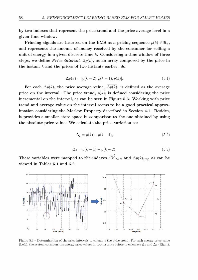
58 5. REINFORCEMENT-LEARNING BASED EMS FOR SMART HOMES
by two indexes that represent the price trend and the price average level in agiven time window.
Princing signals are inserted on the EMS as a pricing sequence p(k) ∈ <+,and represents the amount of money received by the consumer for selling aunit of energy in a given discrete time k. Considering a time window of threesteps, we define Price interval, ∆p(k), as an array composed by the price inthe instant k and the prices of two instants earlier. So:
∆p(k) = [p(k − 2), p(k − 1), p(k)]. (5.1)
For each ∆p(k), the price average value, ∆p(k), is defined as the averageprice on the interval. The price trend,
−−→p(k), is defined considering the price
incremental on the interval, as can be seen in Figure 5.3. Working with pricetrend and average value on the interval seems to be a good practical approx-imation considering the Markov Property described in Section 4.1. Besides,it provides a smaller state space in comparison to the one obtained by usingthe absolute price value. We calculate the price variation as:
∆2 = p(k)− p(k − 1), (5.2)
∆1 = p(k − 1)− p(k − 2). (5.3)
These variables were mapped to the indexes−−→p(k)IND and ∆p(k)IND as can be
viewed in Tables 5.1 and 5.2.
Figure 5.3 – Determination of the price intervals to calculate the price trend. For each energy price value(Left), the system considers the energy price values in two instants before to calculate ∆1 and ∆2 (Right).
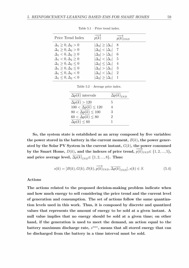
5. REINFORCEMENT-LEARNING BASED EMS FOR SMART HOMES 59
Table 5.1 – Price trend index.
Price Trend Index−−→p(k) −−→
p(k)IND∆1 ≥ 0,∆2 > 0 |∆2| ≥ |∆1| 8∆1 ≥ 0,∆2 > 0 |∆2| < |∆1| 7∆1 < 0,∆2 ≥ 0 |∆2| > |∆1| 6∆1 < 0,∆2 ≥ 0 |∆2| < |∆1| 5∆1 ≥ 0,∆2 ≤ 0 |∆2| ≤ |∆1| 4∆1 ≥ 0,∆2 ≤ 0 |∆2| > |∆1| 3∆1 ≤ 0,∆2 < 0 |∆2| < |∆1| 2∆1 ≤ 0,∆2 < 0 |∆2| ≥ |∆1| 1
Table 5.2 – Average price index.
∆p(k) intervals ∆p(k)IND∆p(k) > 120 5100 < ∆p(k) ≤ 120 480 < ∆p(k) ≤ 100 360 < ∆p(k) ≤ 80 2∆p(k) ≤ 60 1
So, the system state is established as an array composed by five variables:the power stored in the battery in the current moment, B(k), the power gener-ated by the Solar PV System in the current instant, G(k), the power consumedby the Smart Home, D(k), and the indexes of price trend,
−−→p(k)IND∈ {1, 2, ..., 5},
and price average level, ∆p(k)IND∈ {1, 2, ..., 8}. Thus:
s(k) = [B(k), G(k), D(k),−−→p(k)IND,∆p(k)IND], s(k) ∈ S. (5.4)
Actions
The actions related to the proposed decision-making problem indicate whenand how much energy to sell considering the price trend and the current levelof generation and consumption. The set of actions follow the same quantiza-tion levels used in this work. Thus, it is composed by discrete and quantizedvalues that represents the amount of energy to be sold at a given instant. Anull value implies that no energy should be sold at a given time; on otherhand, if the generation is used to meet the demand, an action equal to thebattery maximum discharge rate, smax, means that all stored energy that canbe discharged from the battery in a time interval must be sold.

60 5. REINFORCEMENT-LEARNING BASED EMS FOR SMART HOMES
For each state, there exists a set of admissible actions. Thus, at a givenmoment, one must not choose to sell more energy than the amount available,and if the battery is full, one should not choose to store energy at risk ofexceeding the storage limit. Besides, while there is a limit of selling energyfrom the battery because of the maximum discharge rate, the same limit doesnot exist for the energy generation.
The set of actions is defined as:
A = {0, 0.5, 1, 1.5, ..., smax +GMAX} , (5.5)
where GMAX is the possible maximum amount of energy generated.Be D(k) the user consumption at time k. We define the amount of available
energy Cu(k) as:
Cu(k) = B(k) +G(k)−D(k). (5.6)
Another issue to be discussed is how the selling action can be changeddepending on the user consumption. In our model, the user consumptionchanges the control action to be taken, indicating that we might sell or buyenergy from the grid, as follows.
Thus, we have three cases:
1. If Cu(k) < 0, then the EMS should buy Cu(k) energy;
2. If Cu(k) ≥ 0 and Cu(k) ≤ BMAX, thenAs = {0, ..., Cu(k)};
3. If Cu(k) ≥ 0 and Cu(k) > BMAX, thenAs = {Cu(k)−BMAX , ..., Cu(k)}.
It is worth mentioning that in same states As is also submitted to a restric-tion imposed by the maximum charge/discharge rate of the battery. Thus, inthese cases, there are few admissible actions in order to respect the physicallimits of the storage device.
Reward Function
The reward function maps the current state and the chosen action on a reward,which is a real number. We use a reward function that corresponds to an index
5. REINFORCEMENT-LEARNING BASED EMS FOR SMART HOMES 61
that considers the information of selling energy for a price that is above orbelow the average energy price for a given sequence. Thus,
r(k) = R(s(k), a(k)) = a(k)× (p(k)− p), (5.7)
where p corresponds to the average price data, p(k) is the price at the decisiontime and a ∈ As is the amount of energy to be sold in state s ∈ S.
5.2 Q-Learning and RLbEMS Training Mode
The learning algorithm is the core of the RLbEMS training phase. The Q-Learning Algorithm follows the basic RL approach, in which the proposedsystem acquires knowledge about the environment through trial and error,i.e., it tries actions for a given state and learns about the effect of that actionbased on the evaluation of the obtained reward. However, instead of theclassical on-line approach, in RLbEMS this learning is conducted in an offlinetraining phase, using historical data for experimentation. The RLbEMS Q-Learning algorithm is given in Algorithm 3. The implemented algorithm hasthe same structure of the Algorithm 1, and has as main parts: Definition oftraining parameters, Action selection strategy and Update of system status.Each one of these blocks and their importance for the implementation arediscussed in the following sections.
5.2.1 Definition of system parameters
The first block of the algorithm is where the system data is loaded. In thisblock, the system receives the price, generation and consumption historicaldata and the parameters of the battery. The parameters α and γ are definedas 0.1 and 0.95, respectively. We also define the number of episodes, E, as howmany times the algorithms will use the same historical data for training. Foreach training, the episode is initiated in a different and random initial state.During the tests, we used 3000 as the maximum number of episodes.
After this, the algorithm generates all possible states and actions, consid-ering the given system characteristics. Besides, also in this block the matrixQS×A is initialized as a null matrix and the initial state is defined.
62 5. REINFORCEMENT-LEARNING BASED EMS FOR SMART HOMES
5.2.2 Action selection strategy
After setting the system parameters, the algorithm enters the main loop. Foreach episode, the system chooses a random initial state to start the learningprocess. The initial state is chosen randomly, considering the set of possiblestates defined before. It is worth noting that the set of data acquired in DataAcquisition Mode are synchronized, i.e., there is a generation, demand andprice value for each instant. Considering this and the state definition presentedbefore, choose a random state means just to choose a random initial batteryenergy level, which will be concatenated with the first values of generation,demand and price index from the data set. During the training, this set ofdata evolves sequentially, maintaining data synchronization.
Considering the current system state, the algorithm calculates the amountof energy that is available for selling, Cu. It is important to remember thatRLbEMS only considers selling actions, i.e., there will be only admissibleactions when Cu is greater than 0. Thus, if Cu is less than 0, means that thesystem must buy energy from the grid and, if Cu is equal to 0, means thatthe system meets the energy demand with the energy from the battery andgeneration. In both cases, the system does not have admissible actions to beperformed and it chooses a null action as default.
If Cu is greater than 0, the system must choose to sell or store the availableenergy. As stated before, RLbEMS must learn about the environment and,also, maximize the expected long-term reward. This is generally cited on theliterature as the Exploit × Explore dilemma, when the agent has to choose ineach step whether to explore the environment and acquire more knowledge,or to choose the action that leads to maximize the expected long-term reward.
A way to do this is, at times, to choose the action that maximizes theexpected long-term reward, and at other times to choose a random action inorder to obtain information about the system. The frequency in which thesystem prioritizes to exploit or to explore is known as the rate of exploration,ε, a numerical index that indicates when each option must be followed. Thisindex represents a probability of occurrence and can be defined as fixed orvariable, depending on the studied problem. In cases which ε varies with time,the agent prefers to explore more frequently in the beginning of the learningprocess, choosing and applying random actions, and, as times goes by, theagent starts choosing more frequently to maximize the expected reward.
In this paper we choose to keep ε fixed and equal to 30% during the trainingmode. At each step, the algorithm chooses to explore with a probability of
5. REINFORCEMENT-LEARNING BASED EMS FOR SMART HOMES 63
30% and to exploit with a probability of 70%. In general, choosing to exploremeans to randomly apply an admissible action for a given state; on the otherhand, choosing to exploit means to choose an action that corresponds to themaximum value of the value-action function for a given s(k) ∈ S. However, ifexploiting is chosen for a non-visited state, the algorithm considers a Naïve-Greedy Policy in which the system chooses to sell the energy surplus.
5.2.3 Update of system status
After choosing to exploit or to explore, the next step is to apply the chosenaction, receive the immediate reward and update the system status. Theimmediate reward is calculated as presented in Eq. 5.7 and it is used toupdate the matrix QS×A.
Also, in this block the system evolves to the next state, i.e., the values ofB(k), G(k), D(k),
−−→p(k)IND and ∆p(k)IND are updated. Besides, the new value of
Q(s(k), a(k)) is calculated as indicated in Eq. 4.3 and in Eq. 4.4. Finally, thecurrent state is updated and the learning step is incremented.
The RLbEMS training mode runs until all available price data is visited.After this, the policy is obtained considering Eq. 4.5.

64 5. REINFORCEMENT-LEARNING BASED EMS FOR SMART HOMES
Algorithm 3 Q-Learning for RLbEMS. Define parameters: α,γ;. Load Battery parameters: smax,BMAX ,αB ;. Load data for a specific season: Price data, energy generation, consumption data;. Define finalstep as the size of the price vector;. Define E as the number episodes to be performed;. Define the set of states and actions: S, A;. Initialize the table entry QS×A to zero.while i ≤ E do
Define a random initial state s(k = 0);while k ≤ finalstep do
Observe the current state s(k);Calculate the energy available to sell: Cu(k)← B(k) +G(k)−D(k);if Cu(k) ≤ 0 then
action← 0%System must buy energy from the grid;
if Cu(k) = 0 thenaction← 0%System uses energy from generation and battery to attend the demand;
if Cu(k) > 0 then% Decide for Exploit or Explore:if Choose Exploit then
if Q(s(k),.)=0 thenaction← G(k)−D(k); // Naïve-Greedy Policy%System sells the energy surplus;
elseaction← argmaxa(Q(s(k), a));
elseChoose ExploreDefine an admissible set of actions: Asaction← Choose a random action from As;
a(k)← action;Apply a(k);Calculate the immediate reward: r(k)← a(k)× (p(k)− p);% Evolve the system state:B(k + 1)← (B(k) +G(k)−D(k)− a(k));s(k + 1)← [B(k + 1), G(k + 1), D(k + 1),
−−−−−→p(k + 1)IND,∆p(k + 1)IND];
Update the table entry for Q(s(k), a(k)) as in Eq.4.3 and 4.4;s(k)← s(k + 1);k ← k + 1
i← i+ 1;%% Obtaining the Energy Selling Policyfor ∀sεS do
π(s) = arg maxaεAQ(s, a);
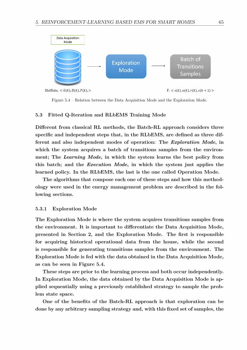
5. REINFORCEMENT-LEARNING BASED EMS FOR SMART HOMES 65
Figure 5.4 – Relation between the Data Acquisition Mode and the Exploration Mode.
5.3 Fitted Q-Iteration and RLbEMS Training Mode
Different from classical RL methods, the Batch-RL approach considers threespecific and independent steps that, in the RLbEMS, are defined as three dif-ferent and also independent modes of operation: The Exploration Mode, inwhich the system acquires a batch of transitions samples from the environ-ment; The Learning Mode, in which the system learns the best policy fromthis batch; and the Execution Mode, in which the system just applies thelearned policy. In the RLbEMS, the last is the one called Operation Mode.
The algorithms that compose each one of these steps and how this method-ology were used in the energy management problem are described in the fol-lowing sections.
5.3.1 Exploration Mode
The Exploration Mode is where the system acquires transitions samples fromthe environment. It is important to differentiate the Data Acquisition Mode,presented in Section 2, and the Exploration Mode. The first is responsiblefor acquiring historical operational data from the house, while the secondis responsible for generating transitions samples from the environment. TheExploration Mode is fed with the data obtained in the Data Acquisition Mode,as can be seen in Figure 5.4.
These steps are prior to the learning process and both occur independently.In Exploration Mode, the data obtained by the Data Acquisition Mode is ap-plied sequentially using a previously established strategy to sample the prob-lem state space.
One of the benefits of the Batch-RL approach is that exploration can bedone by any arbitrary sampling strategy and, with this fixed set of samples, the
66 5. REINFORCEMENT-LEARNING BASED EMS FOR SMART HOMES
algorithm will determine the best possible policy. Considering this, we decidedto apply a random sampling strategy, in which the algorithm chooses, for eachstate, a random action to apply. This strategy is described in Algorithm 4.
In RLbEMS, the batch of samples remains always fixed, i.e., we chose toimplement the classical Batch-RL approach. The use of the Growing Batch-RLmust be done carefully because huge batches may lead to the instability of theSupervised Learning algorithm, worsening the obtained policy. Consideringthis, we use the classical implementation of Batch-RL, in which the batchif fixed. However, periodically, the system restarts and goes to the DataAcquisition Mode, replacing the old batch for a new one and updating thepolicy. In this way, we guarantee the policy will always be updated accordingto the dynamics of the environment and avoid the risk of instability from thealgorithm that makes the approximation of the Q-Function.
Firstly, we load the price, energy generation and consumption data for aspecific season. We also define the number of episodes, E, that represents howmany times the algorithm will use the same historical data to generate newsamples.
The samples from the environment are generated by simply applying thehistorical data sequentially and, for each state, defining a random action toperform. After applying the action, the next state is reached and the imme-diate reward is received. The current state, the action applied, the immediatereward and the next state are inserted in F as a new sample from the en-vironment. This process runs until all historical data are used and for howmany episodes were defined, considering the size of the desired batch definedbefore.
The main result of this step is the batch of samples, F , that will be usedin the Learning Mode to obtain the energy selling policy.
5.3.2 Learning Mode
Once we have the batch of samples from the environment, the next step isto obtain the energy selling policy by entering the RLbEMS Learning Mode.This mode aims to find a function that approximates the value-action functionQ(s, a), ∀s ∈ S, ∀a ∈ A. Thus, the main result of this step is to approximate asurface, QS : S ×A→ Q, that maps each pair state-action to its correspondingQ(s, a) value. The Learning Mode runs the Algorithm 5.
Firstly, we define the basic input of the algorithm. A vector QT is initializedto zero, with the same number of samples as F . This vector will store, in each
5. REINFORCEMENT-LEARNING BASED EMS FOR SMART HOMES 67
iteration, the current updated Q-Value for each pair state-action in F . Wedefine the parameter γ = 0.95, which is the discount factor used to updatethe Q-Value, and the horizon of iteration, that limits how many iterations thealgorithm will run until achieve the desired result.
We also used the convergence criteria dQ defined in Section 4.3 to identifywhen the algorithm converges. Thus, the algorithm runs until the estimationof the Q-Value for each sample of F varies less than 5% from one iteration tothe last one.
The batch of samples, F , is loaded and the function approximator thatis a Supervised Learning Algorithm is defined. As described in Section 4.3,considering experimental results from our benchmarking tests, we chose theRadial Basis Neural Network to approximate the function Q(s, a).
After defining the basic input, the algorithm runs until it reaches the de-sired convergence criteria. The algorithm is composed by two main loops:The Internal Loop, which is responsible for updating the Q-Value in each it-eration for all samples in F , and the External Loop, which is responsible forgenerating a new approximation of the Q-Value function, Q(s, a).
In the Internal Loop, for all samples in F , the algorithm extracts the currentstate and action, s(k) and a(k), the received reward, r(k), and the next state,s(k + 1). Then, the algorithm defines an admissible set of actions for s(k + 1)and calculates, using the last approximation of the Q-Function, an estimate,Q̄, for all admissible actions. Thus, the algorithm updates the Q-Value byusing the maximum value of Q̄, that corresponds to the best admissible actionto be applied in the state s(k+1). This process is repeated for all samples and,as a result, the Internal Loop offers an updated version of the vector QT . Theupdated vector QT is the target value that is used in the Supervised Learningin the External Loop.
A Training Set is defined to be applied in the Supervised Learning Algo-rithm. The inputs are defined as the pairs state-action (s, a) from all samplesin F and the target values as the updated values, QT . This Training Set isapplied in the Radial Basis Neural Network in order to find an approxima-tion for the function Q(s, a). Then, it calculates the convergence criteria, dQ,comparing the vector QT with the one updated in the iteration before.
The algorithm runs until the convergence criteria or until the limit of it-erations are reached. By the end, a Neural Network that represents the bestpossible approximation for the function Q(s, a) considering the fixed batch ofsamples, F , is determined. Then, the algorithm finds the policy by calculating,

68 5. REINFORCEMENT-LEARNING BASED EMS FOR SMART HOMES
for each state s, the final estimate Q̄ for each admissible action. The policy forthe state s is the action a that corresponds to the maximum Q̄. This policywill be used in the RLbEMS Operation Mode, when the system runs with realon-line data.
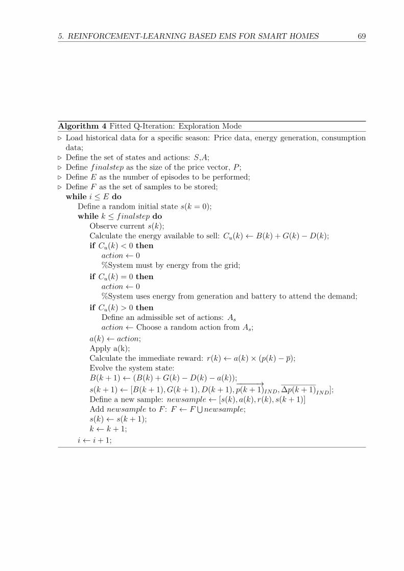
5. REINFORCEMENT-LEARNING BASED EMS FOR SMART HOMES 69
Algorithm 4 Fitted Q-Iteration: Exploration Mode. Load historical data for a specific season: Price data, energy generation, consumptiondata;
. Define the set of states and actions: S,A;
. Define finalstep as the size of the price vector, P ;
. Define E as the number of episodes to be performed;
. Define F as the set of samples to be stored;while i ≤ E do
Define a random initial state s(k = 0);while k ≤ finalstep do
Observe current s(k);Calculate the energy available to sell: Cu(k)← B(k) +G(k)−D(k);if Cu(k) < 0 then
action← 0%System must by energy from the grid;
if Cu(k) = 0 thenaction← 0%System uses energy from generation and battery to attend the demand;
if Cu(k) > 0 thenDefine an admissible set of actions: Asaction← Choose a random action from As;
a(k)← action;Apply a(k);Calculate the immediate reward: r(k)← a(k)× (p(k)− p);Evolve the system state:B(k + 1)← (B(k) +G(k)−D(k)− a(k));s(k + 1)← [B(k + 1), G(k + 1), D(k + 1),
−−−−−→p(k + 1)IND,∆p(k + 1)IND];
Define a new sample: newsample← [s(k), a(k), r(k), s(k + 1)]Add newsample to F : F ← F
⋃newsample;
s(k)← s(k + 1);k ← k + 1;
i← i+ 1;

70 5. REINFORCEMENT-LEARNING BASED EMS FOR SMART HOMES
Algorithm 5 Fitted Q-Iteration: Learning Mode. Initialize a vector QT to zero. The number of elements of QT is equal to the number ofsamples in F ;
. Define parameter: γ;
. Define H as the Horizon to be performed;
. Define εCONV as the convergence criteria for Q̄;
. Load F as the set of samples from the system;
. Define SL as the Supervised Learning algorithm;while (h ≤ H) or (dQ ≥ εCONV ) do
for ∀sample ∈ F doExtract the current state s(k);Extract the current action a(k);Extract the received reward r(k);Extract the next state s(k+1);Define an admissible set of actions for the next state: As(s(k + 1));Estimate Q̄, the Q− V alue of s(k + 1) for all As(s(k + 1));Update the Q−V alue: Q(s(k), a(k)) = r(k)+γ×maxa∈As(s(k+1)) Q̄(s(k + 1), a);QT ← Q(s(k), a(k))
Define TS as a new Training Set: TS=[(s(k), a(k)) QT ], ∀sample ∈ F ;%The pairs (s(k), a(k)) are the inputs and QT are the targets;%%Supervised Learning%Find a new function to estimate Q̄.Apply the new Training Set, TS, to the Supervised Learning Algorithm, SL;Calculate the Convergence Criteria dQ;h← h+ 1;
%% Obtaining the Energy Selling Policy %%for ∀sεS do
π(s) = arg maxaεA Q̄(s, a);%Estimate the Q−V alue for each pair (s(k), a(k)) from S×A by using the function
approximated by SL;

5. REINFORCEMENT-LEARNING BASED EMS FOR SMART HOMES 71
5.4 The RLbEMS Operation Mode
After training, the system enters operation mode, in which the current infor-mation determines the state of the system. Having the current state and theenergy-selling policy learned in the training mode for the current season, theaction is defined and the incremental user profit is calculated, as illustratesthe Algorithm 6.
In case the user bought energy from the power grid, the energy bill isacquired directly from the Smart Meter. Thus, the financial balance is madeby the subtraction between the Profit made and Energy Bill.
Algorithm 6 The RLbEMS Operation Mode. Observe the current season of the year;. Load the learned policy πSEASON ;. Define TotalPR = 0.while TRUE do
Observe the current state s(k);a(k)← πSEASON(s(k))Apply a(k);Calculate the current profit: PR(k) = a(k)× p(k)TotalPR ← TotalPR + PR(k);

72 5. REINFORCEMENT-LEARNING BASED EMS FOR SMART HOMES
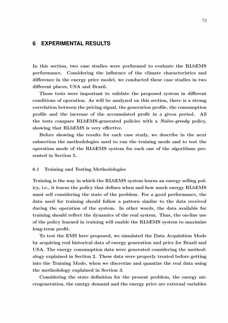
73
6 EXPERIMENTAL RESULTS
In this section, two case studies were performed to evaluate the RLbEMSperformance. Considering the influence of the climate characteristics anddifference in the energy price model, we conducted these case studies in twodifferent places, USA and Brazil.
Those tests were important to validate the proposed system in differentconditions of operation. As will be analyzed on this section, there is a strongcorrelation between the pricing signal, the generation profile, the consumptionprofile and the increase of the accumulated profit in a given period. Allthe tests compare RLbEMS-generated policies with a Naïve-greedy policy,showing that RLbEMS is very effective.
Before showing the results for each case study, we describe in the nextsubsection the methodologies used to run the training mode and to test theoperation mode of the RLbEMS system for each one of the algorithms pre-sented in Section 5.
6.1 Training and Testing Methodologies
Training is the way in which the RLbEMS system learns an energy selling pol-icy, i.e., it learns the policy that defines when and how much energy RLbEMSmust sell considering the state of the problem. For a good performance, thedata used for training should follow a pattern similar to the data receivedduring the operation of the system. In other words, the data available fortraining should reflect the dynamics of the real system. Thus, the on-line useof the policy learned in training will enable the RLbEMS system to maximizelong-term profit.
To test the EMS here proposed, we simulated the Data Acquisition Modeby acquiring real historical data of energy generation and price for Brazil andUSA. The energy consumption data were generated considering the method-ology explained in Section 2. These data were properly treated before gettinginto the Training Mode, when we discretize and quantize the real data usingthe methodology explained in Section 3.
Considering the state definition for the present problem, the energy mi-crogeneration, the energy demand and the energy price are external variables
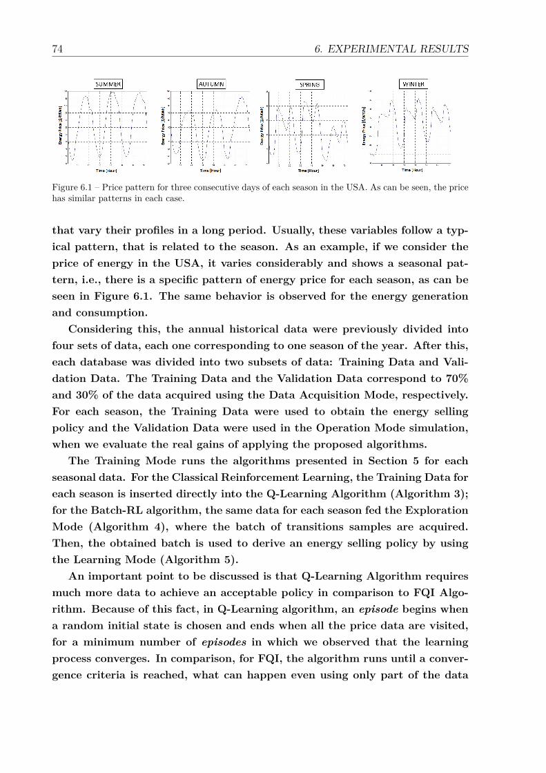
74 6. EXPERIMENTAL RESULTS
Figure 6.1 – Price pattern for three consecutive days of each season in the USA. As can be seen, the pricehas similar patterns in each case.
that vary their profiles in a long period. Usually, these variables follow a typ-ical pattern, that is related to the season. As an example, if we consider theprice of energy in the USA, it varies considerably and shows a seasonal pat-tern, i.e., there is a specific pattern of energy price for each season, as can beseen in Figure 6.1. The same behavior is observed for the energy generationand consumption.
Considering this, the annual historical data were previously divided intofour sets of data, each one corresponding to one season of the year. After this,each database was divided into two subsets of data: Training Data and Vali-dation Data. The Training Data and the Validation Data correspond to 70%and 30% of the data acquired using the Data Acquisition Mode, respectively.For each season, the Training Data were used to obtain the energy sellingpolicy and the Validation Data were used in the Operation Mode simulation,when we evaluate the real gains of applying the proposed algorithms.
The Training Mode runs the algorithms presented in Section 5 for eachseasonal data. For the Classical Reinforcement Learning, the Training Data foreach season is inserted directly into the Q-Learning Algorithm (Algorithm 3);for the Batch-RL algorithm, the same data for each season fed the ExplorationMode (Algorithm 4), where the batch of transitions samples are acquired.Then, the obtained batch is used to derive an energy selling policy by usingthe Learning Mode (Algorithm 5).
An important point to be discussed is that Q-Learning Algorithm requiresmuch more data to achieve an acceptable policy in comparison to FQI Algo-rithm. Because of this fact, in Q-Learning algorithm, an episode begins whena random initial state is chosen and ends when all the price data are visited,for a minimum number of episodes in which we observed that the learningprocess converges. In comparison, for FQI, the algorithm runs until a conver-gence criteria is reached, what can happen even using only part of the data
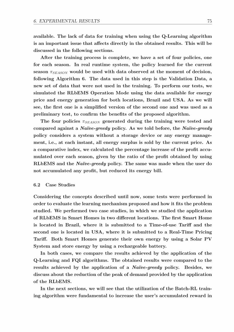
6. EXPERIMENTAL RESULTS 75
available. The lack of data for training when using the Q-Learning algorithmis an important issue that affects directly in the obtained results. This will bediscussed in the following sections.
After the training process is complete, we have a set of four policies, onefor each season. In real runtime system, the policy learned for the currentseason πSEASON would be used with data observed at the moment of decision,following Algorithm 6. The data used in this step is the Validation Data, anew set of data that were not used in the training. To perform our tests, wesimulated the RLbEMS Operation Mode using the data available for energyprice and energy generation for both locations, Brazil and USA. As we willsee, the first one is a simplified version of the second one and was used as apreliminary test, to confirm the benefits of the proposed algorithm.
The four policies πSEASON generated during the training were tested andcompared against a Naïve-greedy policy. As we told before, the Naïve-greedypolicy considers a system without a storage device or any energy manage-ment, i.e., at each instant, all energy surplus is sold by the current price. Asa comparative index, we calculated the percentage increase of the profit accu-mulated over each season, given by the ratio of the profit obtained by usingRLbEMS and the Naïve-greedy policy. The same was made when the user donot accumulated any profit, but reduced its energy bill.
6.2 Case Studies
Considering the concepts described until now, some tests were performed inorder to evaluate the learning mechanism proposed and how it fits the problemstudied. We performed two case studies, in which we studied the applicationof RLbEMS in Smart Homes in two different locations. The first Smart Homeis located in Brazil, where it is submitted to a Time-of-use Tariff and thesecond one is located in USA, where it is submitted to a Real-Time PricingTariff. Both Smart Homes generate their own energy by using a Solar PVSystem and store energy by using a rechargeable battery.
In both cases, we compare the results achieved by the application of theQ-Learning and FQI algorithms. The obtained results were compared to theresults achieved by the application of a Naïve-greedy policy. Besides, wediscuss about the reduction of the peak of demand provided by the applicationof the RLbEMS.
In the next sections, we will see that the utilization of the Batch-RL train-ing algorithm were fundamental to increase the user’s accumulated reward in
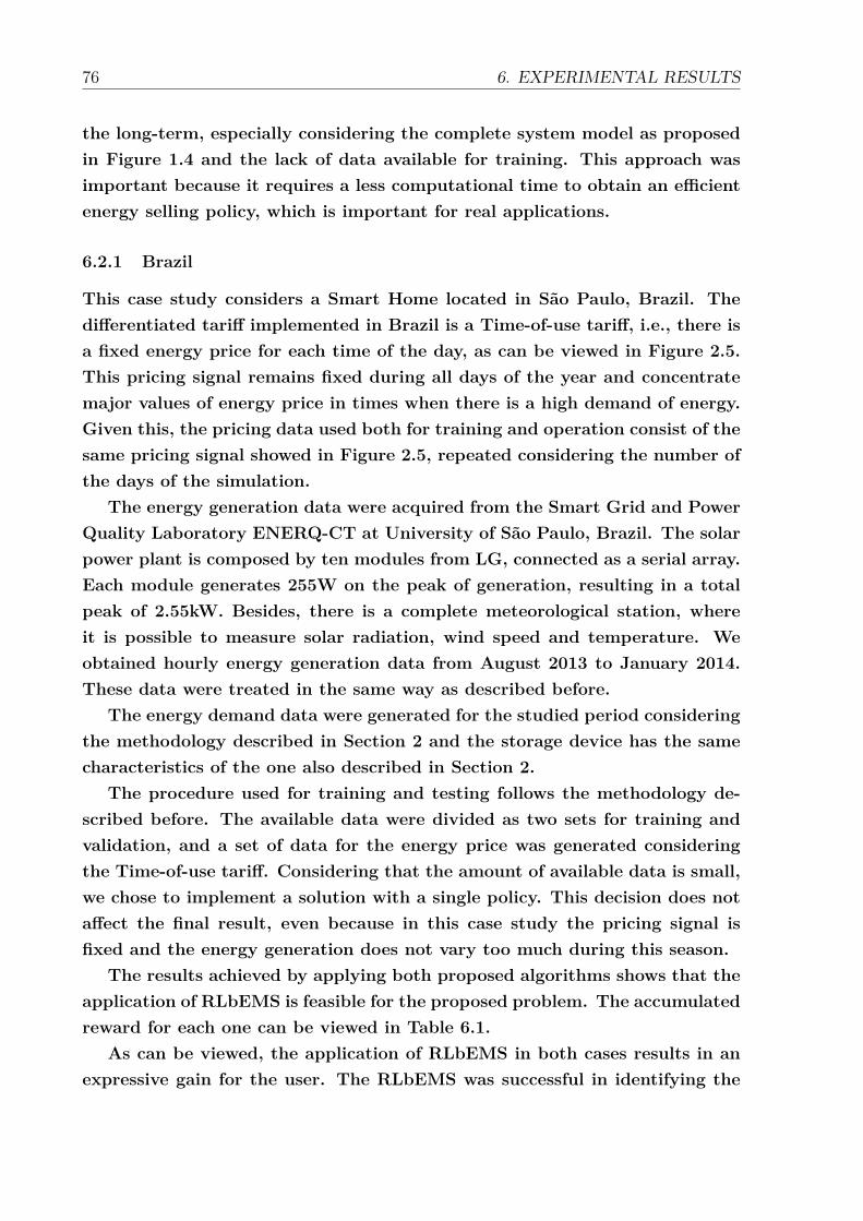
76 6. EXPERIMENTAL RESULTS
the long-term, especially considering the complete system model as proposedin Figure 1.4 and the lack of data available for training. This approach wasimportant because it requires a less computational time to obtain an efficientenergy selling policy, which is important for real applications.
6.2.1 Brazil
This case study considers a Smart Home located in São Paulo, Brazil. Thedifferentiated tariff implemented in Brazil is a Time-of-use tariff, i.e., there isa fixed energy price for each time of the day, as can be viewed in Figure 2.5.This pricing signal remains fixed during all days of the year and concentratemajor values of energy price in times when there is a high demand of energy.Given this, the pricing data used both for training and operation consist of thesame pricing signal showed in Figure 2.5, repeated considering the number ofthe days of the simulation.
The energy generation data were acquired from the Smart Grid and PowerQuality Laboratory ENERQ-CT at University of São Paulo, Brazil. The solarpower plant is composed by ten modules from LG, connected as a serial array.Each module generates 255W on the peak of generation, resulting in a totalpeak of 2.55kW. Besides, there is a complete meteorological station, whereit is possible to measure solar radiation, wind speed and temperature. Weobtained hourly energy generation data from August 2013 to January 2014.These data were treated in the same way as described before.
The energy demand data were generated for the studied period consideringthe methodology described in Section 2 and the storage device has the samecharacteristics of the one also described in Section 2.
The procedure used for training and testing follows the methodology de-scribed before. The available data were divided as two sets for training andvalidation, and a set of data for the energy price was generated consideringthe Time-of-use tariff. Considering that the amount of available data is small,we chose to implement a solution with a single policy. This decision does notaffect the final result, even because in this case study the pricing signal isfixed and the energy generation does not vary too much during this season.
The results achieved by applying both proposed algorithms shows that theapplication of RLbEMS is feasible for the proposed problem. The accumulatedreward for each one can be viewed in Table 6.1.
As can be viewed, the application of RLbEMS in both cases results in anexpressive gain for the user. The RLbEMS was successful in identifying the
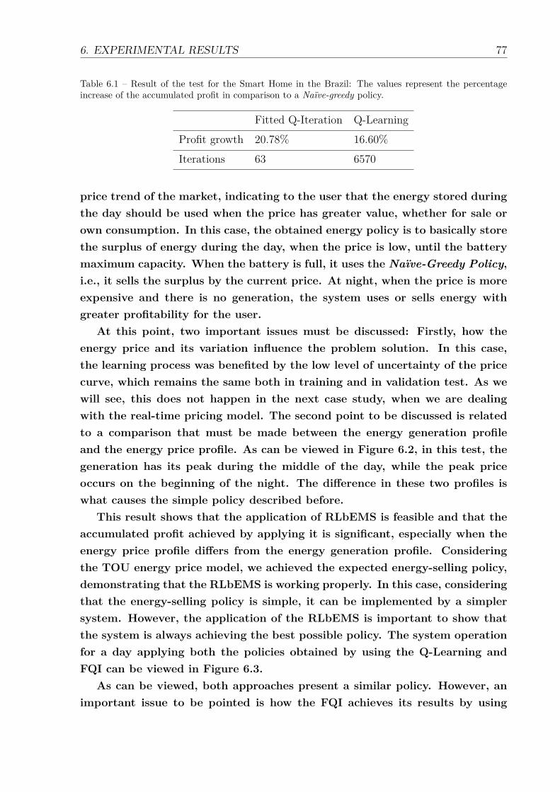
6. EXPERIMENTAL RESULTS 77
Table 6.1 – Result of the test for the Smart Home in the Brazil: The values represent the percentageincrease of the accumulated profit in comparison to a Naïve-greedy policy.
Fitted Q-Iteration Q-LearningProfit growth 20.78% 16.60%Iterations 63 6570
price trend of the market, indicating to the user that the energy stored duringthe day should be used when the price has greater value, whether for sale orown consumption. In this case, the obtained energy policy is to basically storethe surplus of energy during the day, when the price is low, until the batterymaximum capacity. When the battery is full, it uses the Naïve-Greedy Policy,i.e., it sells the surplus by the current price. At night, when the price is moreexpensive and there is no generation, the system uses or sells energy withgreater profitability for the user.
At this point, two important issues must be discussed: Firstly, how theenergy price and its variation influence the problem solution. In this case,the learning process was benefited by the low level of uncertainty of the pricecurve, which remains the same both in training and in validation test. As wewill see, this does not happen in the next case study, when we are dealingwith the real-time pricing model. The second point to be discussed is relatedto a comparison that must be made between the energy generation profileand the energy price profile. As can be viewed in Figure 6.2, in this test, thegeneration has its peak during the middle of the day, while the peak priceoccurs on the beginning of the night. The difference in these two profiles iswhat causes the simple policy described before.
This result shows that the application of RLbEMS is feasible and that theaccumulated profit achieved by applying it is significant, especially when theenergy price profile differs from the energy generation profile. Consideringthe TOU energy price model, we achieved the expected energy-selling policy,demonstrating that the RLbEMS is working properly. In this case, consideringthat the energy-selling policy is simple, it can be implemented by a simplersystem. However, the application of the RLbEMS is important to show thatthe system is always achieving the best possible policy. The system operationfor a day applying both the policies obtained by using the Q-Learning andFQI can be viewed in Figure 6.3.
As can be viewed, both approaches present a similar policy. However, animportant issue to be pointed is how the FQI achieves its results by using
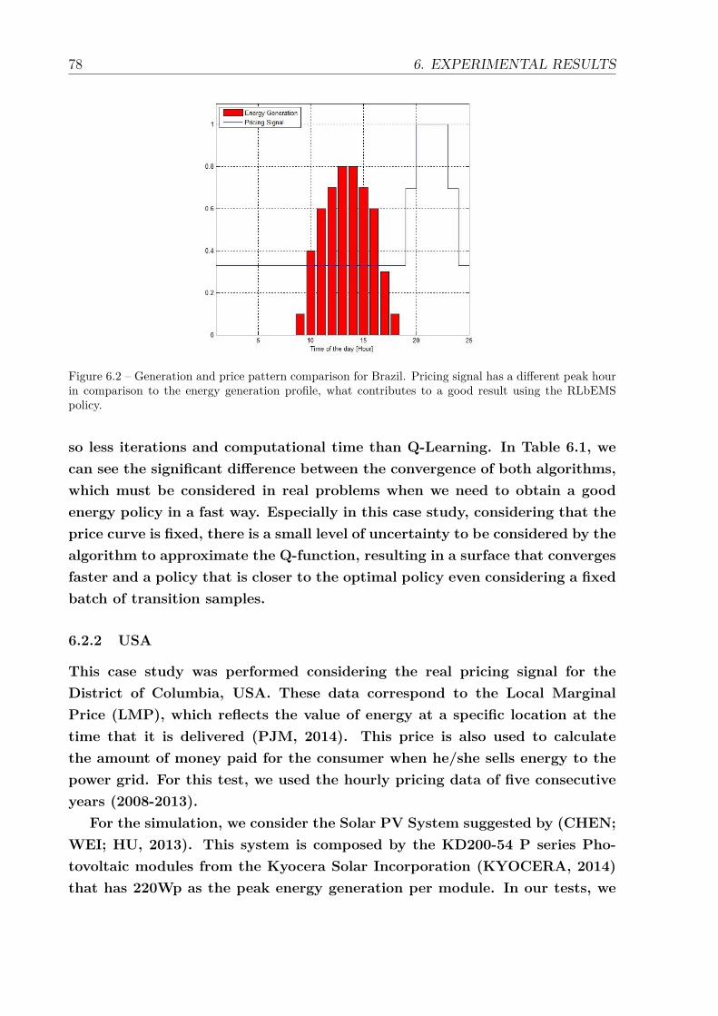
78 6. EXPERIMENTAL RESULTS
Figure 6.2 – Generation and price pattern comparison for Brazil. Pricing signal has a different peak hourin comparison to the energy generation profile, what contributes to a good result using the RLbEMSpolicy.
so less iterations and computational time than Q-Learning. In Table 6.1, wecan see the significant difference between the convergence of both algorithms,which must be considered in real problems when we need to obtain a goodenergy policy in a fast way. Especially in this case study, considering that theprice curve is fixed, there is a small level of uncertainty to be considered by thealgorithm to approximate the Q-function, resulting in a surface that convergesfaster and a policy that is closer to the optimal policy even considering a fixedbatch of transition samples.
6.2.2 USA
This case study was performed considering the real pricing signal for theDistrict of Columbia, USA. These data correspond to the Local MarginalPrice (LMP), which reflects the value of energy at a specific location at thetime that it is delivered (PJM, 2014). This price is also used to calculatethe amount of money paid for the consumer when he/she sells energy to thepower grid. For this test, we used the hourly pricing data of five consecutiveyears (2008-2013).
For the simulation, we consider the Solar PV System suggested by (CHEN;WEI; HU, 2013). This system is composed by the KD200-54 P series Pho-tovoltaic modules from the Kyocera Solar Incorporation (KYOCERA, 2014)that has 220Wp as the peak energy generation per module. In our tests, we
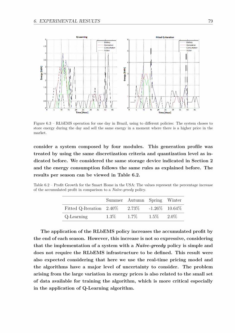
6. EXPERIMENTAL RESULTS 79
Figure 6.3 – RLbEMS operation for one day in Brazil, using to different policies: The system choses tostore energy during the day and sell the same energy in a moment where there is a higher price in themarket.
consider a system composed by four modules. This generation profile wastreated by using the same discretization criteria and quantization level as in-dicated before. We considered the same storage device indicated in Section 2and the energy consumption follows the same rules as explained before. Theresults per season can be viewed in Table 6.2.
Table 6.2 – Profit Growth for the Smart Home in the USA: The values represent the percentage increaseof the accumulated profit in comparison to a Naïve-greedy policy.
Summer Autumn Spring WinterFitted Q-Iteration 2.40% 2.73% -1.26% 10.64%Q-Learning 1.3% 1.7% 1.5% 2.0%
The application of the RLbEMS policy increases the accumulated profit bythe end of each season. However, this increase is not so expressive, consideringthat the implementation of a system with a Naïve-greedy policy is simple anddoes not require the RLbEMS infrastructure to be defined. This result werealso expected considering that here we use the real-time pricing model andthe algorithms have a major level of uncertainty to consider. The problemarising from the large variation in energy prices is also related to the small setof data available for training the algorithm, which is more critical especiallyin the application of Q-Learning algorithm.
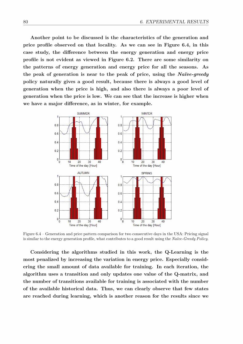
80 6. EXPERIMENTAL RESULTS
Another point to be discussed is the characteristics of the generation andprice profile observed on that locality. As we can see in Figure 6.4, in thiscase study, the difference between the energy generation and energy priceprofile is not evident as viewed in Figure 6.2. There are some similarity onthe patterns of energy generation and energy price for all the seasons. Asthe peak of generation is near to the peak of price, using the Naïve-greedypolicy naturally gives a good result, because there is always a good level ofgeneration when the price is high, and also there is always a poor level ofgeneration when the price is low. We can see that the increase is higher whenwe have a major difference, as in winter, for example.
Figure 6.4 – Generation and price pattern comparison for two consecutive days in the USA: Pricing signalis similar to the energy generation profile, what contributes to a good result using the Naïve-Greedy Policy.
Considering the algorithms studied in this work, the Q-Learning is themost penalized by increasing the variation in energy price. Especially consid-ering the small amount of data available for training. In each iteration, thealgorithm uses a transition and only updates one value of the Q-matrix, andthe number of transitions available for training is associated with the numberof the available historical data. Thus, we can clearly observe that few statesare reached during learning, which is another reason for the results since we

6. EXPERIMENTAL RESULTS 81
chose to use the Naïve-Greedy Policy for states that were not visited duringthe training.
As we exposed before, in each iteration, the FQI uses all the transitionsavailable in a fixed batch to approximate a surface that represents the Q-Function of the problem. Considering this, each transition influences notonly the Q-value related to its state-action pair, but all near transitions areinfluenced by it. This fact results in an algorithm that converges faster for anefficient policy. Moreover, it is not necessary to use the Naïve-Greedy Policyfor unvisited states, since there is an approximation of the Q-value for thesestates. This fact justifies the difference in the policies obtained and, hence,the profit growth for each season.
In Figure 6.5, we can see the RLbEMS operation for two consecutive daysin summer. It is important to note that, when the system is able to identifythe price trend correctly, the policy obtained is similar to the one achieved inthe first case study. The RLbEMS identifies periods of low price and storesenergy to use when there is a peak of price. However, if this peak of priceis not so higher than the low period, the policy loses efficiency. It happensbecause, when the RLbEMS stores energy, it stops selling. If the price dif-ference between these two periods is small, the sale when the price is higherdoes not justify stop selling to store energy when the price would be low. Inthese cases, the application of the RLbEMS policy could lead to a result thatis worse than the application of the Naïve-Greedy Policy, as in Spring, forexample.
Also, we can see in the Figure 6.5 a graph that indicates the hourly energybilling, where positive values are related to energy selling and negative valuesare related to energy buying. As we can see, the RLbEMS also decreases thepeak of demand in the evening, which is one of the main objectives of thiswork. This result is consistent with the assumptions of the Demand ResponseConcept presented in Section 2 and, also, of the Smart Grids.
It is worth mentioning that, considering that the result obtained by the FQIis based in an approximation, it is directly related with the system dynamicsand to how much representative the batch of samples is. As a result, wecan observe that the results from Summer and Autumn are similar, whilethe results are quite different for Winter, that is higher; and for Spring, thatis even negative. If we observe, the energy price in winter varies little incomparison to other seasons, resulting in a similar growth to that achieved inthe first case study. This is different in the Spring, which presents too much
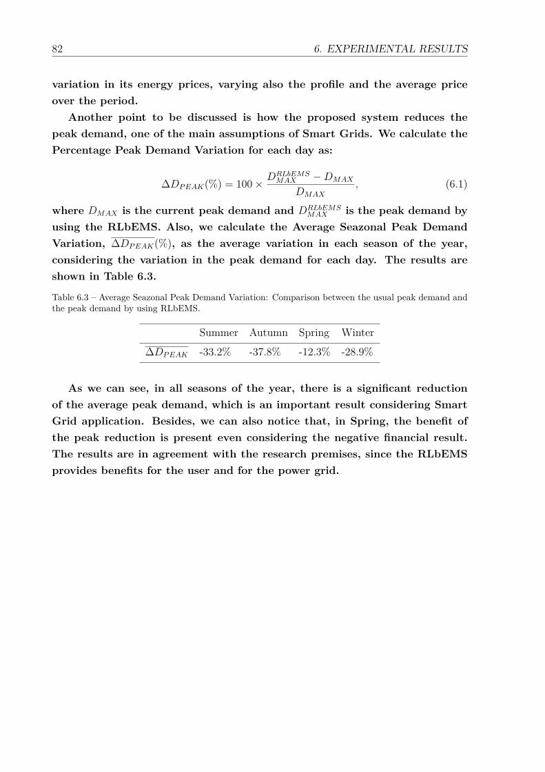
82 6. EXPERIMENTAL RESULTS
variation in its energy prices, varying also the profile and the average priceover the period.
Another point to be discussed is how the proposed system reduces thepeak demand, one of the main assumptions of Smart Grids. We calculate thePercentage Peak Demand Variation for each day as:
∆DPEAK(%) = 100× DRLbEMSMAX −DMAX
DMAX
, (6.1)
where DMAX is the current peak demand and DRLbEMSMAX is the peak demand by
using the RLbEMS. Also, we calculate the Average Seazonal Peak DemandVariation, ∆DPEAK(%), as the average variation in each season of the year,considering the variation in the peak demand for each day. The results areshown in Table 6.3.
Table 6.3 – Average Seazonal Peak Demand Variation: Comparison between the usual peak demand andthe peak demand by using RLbEMS.
Summer Autumn Spring Winter
∆DPEAK -33.2% -37.8% -12.3% -28.9%
As we can see, in all seasons of the year, there is a significant reductionof the average peak demand, which is an important result considering SmartGrid application. Besides, we can also notice that, in Spring, the benefit ofthe peak reduction is present even considering the negative financial result.The results are in agreement with the research premises, since the RLbEMSprovides benefits for the user and for the power grid.
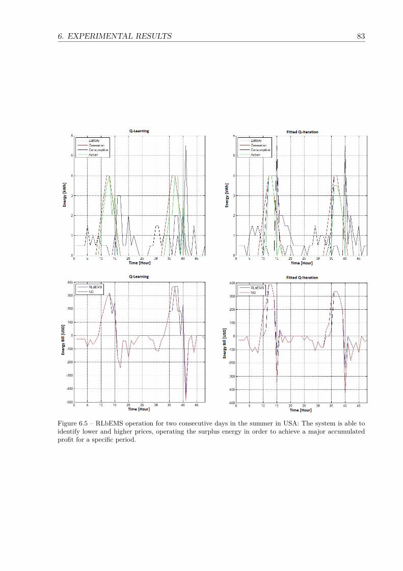
6. EXPERIMENTAL RESULTS 83
Figure 6.5 – RLbEMS operation for two consecutive days in the summer in USA: The system is able toidentify lower and higher prices, operating the surplus energy in order to achieve a major accumulatedprofit for a specific period.

84 6. EXPERIMENTAL RESULTS
85
7 CONCLUDE
This research proposed a Reinforcement Learning-based Energy ManagementSystem called RLbEMS that maximizes the rewards achieved by residentialconsumers in their energy operation, considering a Smart Home that generatesits own energy and that has a storage device. Besides, this Smart Homereceives a pricing signal that varies during the time of the day, which justifiesthe use of a RLbEMS solution that, for each state of the system, must choosebetween selling/using energy at the current price or store energy to sell/useit at a better time in the future. The system has two modes of operation: thetraining mode uses historical data to obtain a selling policy for each seasonof the year and the operation mode applies the learned policies consideringthe sequential real-time data. The problem was modeled as a MDP and RLalgorithms were used to solve the problem.
Two different RL approaches were compared, the classical on-line RL andthe Batch-RL. The Q-Learning algorithm was used and, despite the lack ofavailable data, achieved a good performance. Nevertheless, the large compu-tational time for obtaining an energy selling policy complicating its applicationin real problems. In the meantime, the result obtained using the Fitted Q-Iteration proved that the solution using a RL approach is feasible for realapplication. We achieved a good energy selling policy even considering thelack of data. Besides, the Fitted Q-Iteration converges faster than Q-Learning,which is another characteristic that indicates this algorithm as the most qual-ified for the real implementation of RLbEMS.
In order to validate the developed system, we analyzed two case studies.The first case study considers a Smart Home in the Brazil, where we obtaineda maximum gain of 20.78% for RLbEMS in comparison to a Naïve-greedypolicy. In this case study, the energy generation profile differs considerablyfrom the pricing signal, justifying the usage of storage devices consideringthat the system chooses to store energy when the price is low and to sell thestored energy when the price is high. Besides, the energy price is a fixed dailyprofile, which means less uncertainty for the EMS deal with. The second casestudy considers a Smart Home in USA, where we obtained a maximum gainof 10.64% for the application of RLbEMS. The reduction of the user’s gain isjustified by the great similarity between the energy generation pattern and the
86 7. CONCLUDE
pricing signal for this locality. Besides, this location considers a energy pricethat varies in each our, which corresponds to a higher level of uncertainty incomparison to the first case study. Also, the lack of historical data affects theresults because difficults the convergence of the algorithms used.
Another important result achieved by the RLbEMS was the reduction ofthe peak of demand, which is one of the main objectives of the implementationof Smart Grids. The application of RLbEMS by using the FQI algorithmproduces a decrease in the peak of demand that is higher than 30%, in themost cases. This is an important issue and allows the optimal operation ofthe power grid.
Considering the best results achieved by the application of RLbEMS byusing the FQI algorithm, we can list:
1. Financial: The system reduces the Solar PV System payback time, evenconsidering the investment in storage devices and in the EMS.
2. Energetic: The system provides a reduction of the peak demand, whichresults in a small use of thermoelectrics and in a lower energy cost.
3. Power Grid: A more active participation of the end user in the powersupply. Besides, it provides an optimal use of the power grid, reducingthe costs of the utilities.
Another major contribution of this research is to propose a new approachfor modeling and solving the energy management problem in Smart Homes.We propose a system that was tested with real energy generation and energyprice data for two different places and, considering that these data depend onthe location, we have showed that the proposed system can be used in situa-tions characterized by different levels of uncertainty. The results demonstratethat the modeling using MDP and the solution using RL are feasible, despitethe limitations such as the small amount of data available for training. Thesolutions proposed in the literature describe the system in a different way and,in the most cases, the tests realized do not consider real generation and pricedata. Moreover, the proposed solution guarantees the degree of freedom ofthe user, since it optimizes the usage of energy sources considering only theprice informed. Thus, the user does not have restrictions regarding the use ofappliances in his/her home. We believe this degree of freedom is essential sothat a solution as proposed in the article can be incorporated into the routineof the user, leading to the popularization of systems like this.
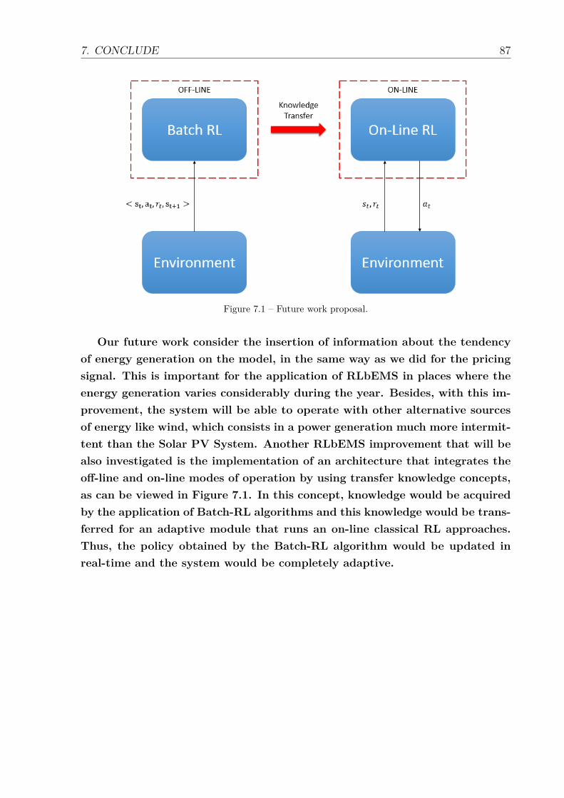
7. CONCLUDE 87
Figure 7.1 – Future work proposal.
Our future work consider the insertion of information about the tendencyof energy generation on the model, in the same way as we did for the pricingsignal. This is important for the application of RLbEMS in places where theenergy generation varies considerably during the year. Besides, with this im-provement, the system will be able to operate with other alternative sourcesof energy like wind, which consists in a power generation much more intermit-tent than the Solar PV System. Another RLbEMS improvement that will bealso investigated is the implementation of an architecture that integrates theoff-line and on-line modes of operation by using transfer knowledge concepts,as can be viewed in Figure 7.1. In this concept, knowledge would be acquiredby the application of Batch-RL algorithms and this knowledge would be trans-ferred for an adaptive module that runs an on-line classical RL approaches.Thus, the policy obtained by the Batch-RL algorithm would be updated inreal-time and the system would be completely adaptive.

88 7. CONCLUDE
89
REFERENCES
ABRADEE. Associacao Brasileira de Distribuidores de Energia Eletrica.2014. <http://www.abradee.com.br>. Accessed: 2014-02-01.
ALBADI, M. H.; EL-SAADANY, E. Demand response in electricity markets:An overview. In: Power Engineering Society General Meeting, 2007. IEEE.[S.l.: s.n.], 2007. p. 1–5. ISSN 1932-5517.
ANEEL. Resolucao Normativa 482 - Agencia Nacional de Energia Eletrica(ANEEL). 2014. <http://www.aneel.gov.br/cedoc/ren2012482.pdf>.Accessed: 2013-04-01.
ATZENI, I.; ORDONEZ, L.; SCUTARI, G.; PALOMAR, D.; FONOLLOSA,J. Demand-side management via distributed energy generation and storageoptimization. Smart Grid, IEEE Transactions on, v. 4, n. 2, p. 866–876,June 2013. ISSN 1949-3053.
BALIJEPALLI, V.; PRADHAN, V.; KHAPARDE, S.; SHEREEF, R. M.Review of demand response under smart grid paradigm. In: InnovativeSmart Grid Technologies - India (ISGT India), 2011 IEEE PES. [S.l.: s.n.],2011. p. 236–243.
BELLMAN, R. Dynamic Programming. 1. ed. Princeton, NJ, USA:Princeton University Press, 1957.
BERLINK, H.; COSTA, A. R. Aplicação de aprendizado por reforço naotimização da venda de energia na geração distribuída. ENIAC 2013 -Encontro Nacional de Inteligência Artificial e Computacional, 2013.
BERLINK, H.; KAGAN, N.; COSTA, A. R. Intelligent decision-making forsmart home energy management. Journal of Intelligent & Robotic Systems,Springer Netherlands, p. 1–24, 2014. ISSN 0921-0296.
BUENO, E.; UTUBEY, W.; HOSTT, R. Evaluating the effect of the whitetariff on a distribution expansion project in brazil. In: Innovative SmartGrid Technologies Latin America (ISGT LA), 2013 IEEE PES ConferenceOn. [S.l.: s.n.], 2013. p. 1–8.
CARPINELLI, G.; CELLI, G.; MOCCI, S.; MOTTOLA, F.; PILO, F.;PROTO, D. Optimal integration of distributed energy storage devices insmart grids. Smart Grid, IEEE Transactions on, v. 4, n. 2, p. 985–995, June2013. ISSN 1949-3053.
CHEN, C.; KISHORE, S.; WANG, Z.; ALIZADEH, M.; SCAGLIONE,A. How will demand response aggregators affect electricity markets? a
90 REFERENCES
cournot game analysis. In: Communications Control and Signal Processing(ISCCSP), 2012 5th International Symposium on. [S.l.: s.n.], 2012. p. 1–6.
CHEN, X.; WEI, T.; HU, S. Uncertainty-aware household appliancescheduling considering dynamic electricity pricing in smart home. SmartGrid, IEEE Transactions on, v. 4, n. 2, p. 932–941, June 2013. ISSN1949-3053.
CHEN, Z.; WU, L.; FU, Y. Real-time price-based demand responsemanagement for residential appliances via stochastic optimization and robustoptimization. Smart Grid, IEEE Transactions on, v. 3, n. 4, p. 1822–1831,Dec 2012. ISSN 1949-3053.
DOE. U.s. department of energy. the smart grid: An introduction. 2009.
DRUCKER HARRIS; BURGES, C. J. C. K. L. S. A. J.; VAPNIK, V. N.Support vector regression machines. Advances in Neural InformationProcessing Systems 9, MIT Press, p. 155–161, 1997.
DUSPARIC, I.; HARRIS, C.; MARINESCU, A.; CAHILL, V.; CLARKE,S. Multi-agent residential demand response based on load forecasting. In:Technologies for Sustainability (SusTech), 2013 1st IEEE Conference on.[S.l.: s.n.], 2013. p. 90–96.
ERNST, D.; GEURTS, P.; WEHENKEL, L.; LITTMAN, L. Tree-basedbatch mode reinforcement learning. Journal of Machine Learning Research,v. 6, p. 503–556, 2005a.
HAMMOUDEH, M.; MANCILLA-DAVID, F.; SELMAN, J.; PAPANTONI-KAZAKOS, P. Communication architectures for distribution networks withinthe smart grid initiative. In: Green Technologies Conference, 2013 IEEE.[S.l.: s.n.], 2013. p. 65–70. ISSN 2166-546X.
HASHMI, M.; HANNINEN, S.; MAKI, K. Survey of smart grid concepts,architectures, and technological demonstrations worldwide. In: InnovativeSmart Grid Technologies (ISGT Latin America), 2011 IEEE PESConference on. [S.l.: s.n.], 2011. p. 1–7.
JARDINI, J.; RAMOS, D.; MARTINI, J. C.; REIS, L.; TAHAN, C. Brazilianenergy crisis. Power Engineering Review, IEEE, v. 22, n. 4, p. 21–24, April2002. ISSN 0272-1724.
KEEN, P. Quantifying the effect of demand response on electricity markets.Cambridge, Center for Information Systems Research, 1980.
KIM, T.; POOR, H. Scheduling power consumption with price uncertainty.Smart Grid, IEEE Transactions on, v. 2, n. 3, p. 519–527, Sept 2011. ISSN1949-3053.
REFERENCES 91
KYOCERA. Kyocera Solar, Data Sheet of KD200-54 P Series PV Modules[On- line]. 2014. <http://www.kyocerasolar.com/assets/001/5124.pdf>.Accessed: 2014-11-01.
LIU, W.-H. Analytics and information integration for smart grid applications.In: Power and Energy Society General Meeting, 2010 IEEE. [S.l.: s.n.],2010. p. 1–3. ISSN 1944-9925.
MCGRANAGHAN, M.; DOLLEN, D. V.; MYRDA, P.; GUNTHER, E.Utility experience with developing a smart grid roadmap. In: Power andEnergy Society General Meeting - Conversion and Delivery of ElectricalEnergy in the 21st Century, 2008 IEEE. [S.l.: s.n.], 2008. p. 1–5. ISSN1932-5517.
MOHSENIAN-RAD, A.-H.; WONG, V.; JATSKEVICH, J.; SCHOBER,R.; LEON-GARCIA, A. Autonomous demand-side management based ongame-theoretic energy consumption scheduling for the future smart grid.Smart Grid, IEEE Transactions on, v. 1, n. 3, p. 320–331, Dec 2010. ISSN1949-3053.
MPPTSOLAR. MPPT Solar [On-line]. 2014. <http://www.mpptsolar.com/pt/baterias-serie-paralelo.html>. Accessed: 2014-11-01.
NEOSOLAR. Neosolar - Sistemas de Energia Fotovoltaica e seus compo-nentes [On-line]. 2014. <http://www.neosolar.com.br/aprenda/saiba-mais/sistemas-de-energia-solar-fotovoltaica-e-seus-componentes>. Accessed:2014-11-01.
NIST. National Institute of Standards and Technology (NIST). 2014.<http://www.nist.gov/smartgrid/>. Accessed: 2014-06-01.
O’NEILL, D.; LEVORATO, M.; GOLDSMITH, A.; MITRA, U. Residentialdemand response using reinforcement learning. In: Smart Grid Communi-cations (SmartGridComm), 2010 First IEEE International Conference on.[S.l.: s.n.], 2010. p. 409–414.
ORMONEIT, D.; GLYNN, P. Kernel-based reinforcement learning inaverage-cost problems. Automatic Control, IEEE Transactions on, v. 47,n. 10, p. 1624–1636, Oct 2002. ISSN 0018-9286.
PALENSKY, P.; DIETRICH, D. Demand side management: Demandresponse, intelligent energy systems, and smart loads. Industrial Informatics,IEEE Transactions on, v. 7, n. 3, p. 381–388, Aug 2011. ISSN 1551-3203.
PARK, J.; SANDBERG, I. Universal approximation using radial-basis-function networks. MIT - Neural Computation, Springer Netherlands, 1991.ISSN 0899-7667.
92 REFERENCES
PARVANIA, M.; FOTUHI-FIRUZABAD, M.; SHAHIDEHPOUR, M.Demand response participation in wholesale energy markets. In: Power andEnergy Society General Meeting, 2012 IEEE. [S.l.: s.n.], 2012. p. 1–4. ISSN1944-9925.
PJM. PJM monthly locational marginal pricing [On-line]. 2014. <http://www.pjm.com/markets-and-operations/energy/real-time/monthlylmp.aspx>.Accessed: 2014-02-01.
POWER, D. J. Decision support systems: concepts and resources formanagers. Quorum Books,Westport, Conn., 2002.
PROCEL. Dicas de Economia de Energia - Programa Nacional deConservacao da Energia Eletrica. 2014. <http://www.procelinfo.com.br>.Accessed: 2014-08-01.
RIEDMILLER, M.; HAFNER, R.; LANGE, S.; LAUER, M. Learning todribble on a real robot by success and failure. In: Robotics and Automation,2008. ICRA 2008. IEEE International Conference on. [S.l.: s.n.], 2008. p.2207–2208. ISSN 1050-4729.
RUSSELL, S. J.; NORVIG, P.; CANDY, J. F.; MALIK, J. M.; EDWARDS,D. D. Artificial Intelligence: A Modern Approach. Upper Saddle River, NJ,USA: Prentice-Hall, Inc., 1996. ISBN 0-13-103805-2.
SHISHEBORI, A.; KIAN, A. Risk analysis for distribution company energyprocurement with pool market, dgs and demand response. In: ElectricalEngineering (ICEE), 2010 18th Iranian Conference on. [S.l.: s.n.], 2010. p.949–954.
SOL HENK G., T. C. A. d. V. R. P. F. Expert systems and artificialintelligence in decision support systems. Second Mini Euroconference,Lunteren, The Netherlands, 1987.
STEPHENS, W.; MIDDLETON, T. Why has the uptake of decision supportsystems been so poor? Crop-soil simulation models in developing countries,p. 129–130, 2002.
SU, C.-L.; KIRSCHEN, D. Quantifying the effect of demand response onelectricity markets. Power Systems, IEEE Transactions on, v. 24, n. 3, p.1199–1207, Aug 2009. ISSN 0885-8950.
SUTTON, R. S.; BARTO, A. G. Introduction to Reinforcement Learning.1st. ed. Cambridge, MA, USA: MIT Press, 1998. ISBN 0262193981.
T. JAY E., T.-P. L. E. Decision support systems and intelligent systems.Prentice Hall, 2008.
ULUSKI, R. The role of advanced distribution automation in the smart grid.In: Power and Energy Society General Meeting, 2010 IEEE. [S.l.: s.n.],2010. p. 1–5. ISSN 1944-9925.

REFERENCES 93
WANG, Z.; GU, C.; LI, F.; BALE, P.; SUN, H. Active demand responseusing shared energy storage for household energy management. Smart Grid,IEEE Transactions on, v. 4, n. 4, p. 1888–1897, Dec 2013. ISSN 1949-3053.
WATKINS, C. J. C. H. Learning from Delayed Rewards. Cambridge, UK:[s.n.], 1989.
WATTS, D.; ARIZTIA, R. The electricity crises of california, brazil andchile: lessons to the chilean market. In: Power Engineering 2002 LargeEngineering Systems Conference on, LESCOPE 02. [S.l.: s.n.], 2002. p.7–12.
WRIGHT A; SITTIG, D. A framework and model for evaluating clinicaldecision support architectures q. Journal of Biomedical Informatics 41,2008.