Embed Size (px)
Citation preview
Journal of Classification 27 (2009) DOI: 10.1007/s00357-010-
_______________
The authors express their gratitude to the anonymous referees whose multiple com-ments have been taken into account in our revisions of the paper.
Authors’ Address: School of Computer Science and Information Systems, Birkbeck University of London, London, UK, e-mail: {mingtsoc, Mirkin}@dcs.bbk.ac.uk
Intelligent Choice of the Number of Clusters in K-Means Clustering: An Experimental Study with Different Cluster Spreads Mark Ming-Tso Chiang Birkbeck University of London Boris Mirkin Birkbeck University of London
Abstract: The issue of determining “the right number of clusters” in K-Means has attracted considerable interest, especially in the recent years. Cluster intermix ap-pears to be a factor most affecting the clustering results. This paper proposes an ex-perimental setting for comparison of different approaches at data generated from Gaussian clusters with the controlled parameters of between- and within-cluster spread to model cluster intermix. The setting allows for evaluating the centroid re-covery on par with conventional evaluation of the cluster recovery. The subjects of our interest are two versions of the “intelligent” K-Means method, ik-Means, that find the “right” number of clusters by extracting “anomalous patterns” from the data one-by-one. We compare them with seven other methods, including Hartigan’s rule, averaged Silhouette width and Gap statistic, under different between- and within- cluster spread-shape conditions. There are several consistent patterns in the results of our experiments, such as that the right K is reproduced best by Hartigan’s rule – but not clusters or their centroids. This leads us to propose an adjusted version of iK-Means, which performs well in the current experiment setting. Keywords: K-Means clustering; Number of clusters; Anomalous pattern; Hartigan’s rule; Gap statistic.
M. Ming-Tso Chiang and B. Mirkin
1. Introduction
The problem of determining “the right number of clusters” attracts considerable interest in the literature (for reviews, see Jain and Dubes (1988), Dudoit and Fridlyand (2002), Mirkin (2005), Steinley (2006) and Section 3 below). Most published papers propose a procedure for estimat-ing the number of clusters and experimentally compare it to some other methods. Some authors do more comprehensive experiments and either arrive at some winning procedures, like Milligan and Cooper (1985) in their seminal study of 30 indexes for cutting cluster hierarchies, or obtain inconclusive results like Hardy (1996) and Dimitraidou, Dolnicar and Weingessel (2002). Steinley and Henson (2005) pointed out that it is very important, in experiments with simulated data, to maintain a degree of cluster overlap to be able to derive any realistic conclusions, which was not the case in previously published experimental studies. They propose a model for data generation with overlapping clusters, which however con-tains too many parameters and can model only one-dimensional intersec-tions. In a follow-up experimental study of different initialization strate-gies, Steinley and Brusco (2007) come to the conclusion that cluster over-lap, in their setting, is the property of generated data that most affects the cluster recovery.
This paper focuses on experimental comparison of various options for selecting the number of clusters in the most popular partitioning method, K-Means. Specifically, we analyze the performance of an “intelli-gent” version of K-Means, iK-Means (Mirkin 2005), which initializes K-Means with the so-called Anomalous pattern (AP) clusters that are furthest away from the origin of the feature space. This method is compared with a number of other methods, each attempting at selection of the right number of clusters from a range of numbers, by using a specially designed index. To choose these other methods, we undertake a systematic review of more than a dozen recently published methods for identifying the right number of clusters in K-Means, as well as some earlier experimentally supported recipes.
We utilize the conventional Gaussian distribution as the cluster generation model, with its parameters, the mean point and covariance matrix, being naturally interpretable in terms of location and shape, respectively. The cluster “overlap”, in this setting, can be modelled by combining two factors, the within-cluster spread and between-cluster spread. It should be pointed out that the term “overlap” here should not be understood as the set-theoretic intersection but rather intermix, due to the probabilistic nature of the data generator. In this setting, the set-theoretic intersection interpretation of the overlap is not relevant, because the generated, as well as recovered, clusters always form a partition. Yet the
Number of Clusters in K-Means Clustering
clusters can and do intermix spatially (see more detail on this in Section 4.1.D).
Because of both the usage of Gaussians in the data generation and specifics of K-Means, which finds both clusters and their centroids, we can compare methods’ performances not only in terms of the recovery of the number of clusters or clusters themselves, as usual, but also in terms of their capabilities in recovering cluster centroids. This is not a trivial matter, because cluster centroids may be as, or even more, important as clusters themselves: they may represent the conceptual, or intensional, meaning of clusters. An important issue emerging in the analysis of centroid recovery is whether the cluster sizes should be taken into account or not, the latter under the assumption that the centroid of a small cluster, containing just a few entities, can be as important as the centroid of a large cluster. We sug-gest that this issue can be addressed by comparing the clustering methods’ centroid recovery performances with their cluster recovery performances. Since these two performances should go in line, that method of measuring the centroid recovery performance that makes it more similar to the cluster recovery performance should be preferred. In our experiments, the un-weighted centroids win indeed.
Another experimental finding is that the number of clusters is best reproduced by Hartigan’s (1975) method, though the method’s perform-ance regarding the cluster or centroid recovery is less impressive. On the other hand, iK-Means performs rather well in terms of the cluster and cen-troid recovery, but may drastically overestimate the number of clusters, especially at the small between-cluster spreads. This leads us to propose an adjusted version of iK-Means, which performs rather well on all three counts—the number of clusters, the cluster recovery and the centroid re-covery.
The paper is organized as follows. Generic versions of K-Means and intelligent K-Means are described in Section 2. Section 3 contains a review of methods for finding the right K in K-Means in the published literature. We distinguish between five approaches as based primarily on: cluster variance, within-cluster cohesion versus between-cluster separation, con-sensus distribution, hierarchical clustering, and resampling. The setting of our experiments at the comparison of nine selected methods for finding the “right clustering”—the data sizes, the cluster shapes, the within- and be-tween-cluster spread parameters, and evaluation criteria—is described in Section 4. Basically, we deal with different cluster intermix settings result-ing from combining two types of the between-cluster spread and two mod-els of the within-cluster shape and three models of the within-cluster spread. Section 5 presents results of our experiments in tables containing the evaluation criteria values, averaged over multiple data generations at each of the settings, along with issues raised before the experiments and
M. Ming-Tso Chiang and B. Mirkin
answers to them coming from the results. The experiments have been con-ducted in two instalments so that the second series features expanded sets of both methods and generated data structures. Section 6 concludes the paper.
2. K-Means and Intelligent K-Means
2.1 Generic K-Means
K-Means clustering method, conventionally, applies to a dataset in-volving a set of N entities, I, set of M features, V, and an entity-to-feature matrix Y=(yiv), where yiv is the value of feature vV at entity iI. The method produces a partition S={S1, S2,…, SK} of I in K non-empty non-overlapping classes Sk, referred to as clusters, each with a centroid ck=(ckv), an M-dimensional vector in the feature space (k=1,2,…K). Centroids form the set C={c1, c2,…, cK}. The criterion, alternatingly minimized by the method, is the sum of within-cluster distances to centroids:
W(S, C) =1
( , )k
K
kk i S
d i c= ŒÂ (1)
where d is a distance measure, typically the squared Euclidean distance or Manhattan distance. In the former case criterion (1) is referred to as the squared error criterion and in the latter, the absolute error criterion.
Given K M-dimensional vectors ck as cluster centroids, the algo-rithm updates clusters Sk according to the Minimum distance rule: For each entity i in the data table, its distances to all centroids are calculated and the entity is assigned to its nearest centroid. Given clusters Sk, centroids ck are updated according to the distance d in criterion (1), k=1, 2, …, K. Specifi-cally, ck is calculated as the vector of within-cluster averages if d in (1) is the squared Euclidean distance and as of within-cluster medians if d is Manhattan distance. This process is reiterated until clusters Sk stabilize. This algorithm is sometimes referred to as Batch K-Means or Straight K-Means.
When the distance d in (1) is indeed the squared Euclidean distance, K-Means can be seen as an implementation of the alternating optimization procedure for maximization of the maximum likelihood under the assumed mixture of “spherical” Gaussian distributions model, in which all covari-ance matrices are equal to a diagonal matrix 2I where I is the identity ma-trix and 2 the variance value (Hartigan 1975; Banfield and Raftery 1993; McLachlan and Peel 2000). Another, somewhat lighter interpretation comes from the data mining paradigm, in which (1) is but the least-squares criterion for approximation of the data with a data recovery clustering
Number of Clusters in K-Means Clustering
model (Mirkin 1990, 2005; Steinley 2006) that states that every entry yiv in the data matrix (i denotes an entity and v a feature), can be presented as approximated by the “hidden” set of clusters S={S1, S2,…, SK} and their centers C={c1, c2,…, cK} through equations
1
,K
iv kv ik ivk
y c s e=
= +Â (2)
where sk=(sik) is Sk membership vector in which sik=1 if iSk and sik=0 otherwise, and eiv are residuals to be minimized over unknown ck and sk (k=1,2,…,K). Criterion (1) is the least-squares or least-moduli fitting crite-rion for model (2) if d in (1) is the squared Euclidean distance or Manhat-tan distance, respectively. More on K-Means and its history can be found in reviews by Steinley (2006) and Bock (2007).
What is important in this is that, both K and initial centroids are to be pre-specified to initialize the method. The algorithm converges to a lo-cal minimum of criterion (1) rather fast, and the goodness of the stationary solution much depends on the initialization.
2.2 Choosing K with the Intelligent K-Means
A version of K-Means in which the number of clusters and initial centroids are determined with a procedure targeting “anomalous patterns” as the candidates for the initial centroids has been described as “intelligent K-Means” algorithm, iK-Means in Mirkin (2005). It initializes K-Means by standardizing the data in such a way that the origin is put into a “refer-ence” point, usually the gravity center of all the data points, and iterating then the so-called Anomalous Pattern (AP) algorithm which builds clusters one by one, starting from that which is the furthest away from the origin, and reapplying the process to the entities remaining not clustered yet. This is a version of the so-called Principal Cluster Analysis approach that emu-lates the one-by-one strategy of the Principal component analysis applied to model (2): an AP pattern is a cluster derived from model (2) at K=1 in such a way that it maximally contributes to the data scatter (Mirkin 1990). The fact that AP cluster is far away from the reference point conforms to the notion of interestingness in data mining: the farther from normal, the more interesting (Fayyad, Piatestsky-Shapiro, Smyth, and Uthurusamy 1996). Those of the found clusters that are too small, that is, singletons, are removed from the set, and the centroids of the rest are taken as the initial setting for K-Means.
The AP algorithm starts from that entity, which is the farthest from the origin, as the initial centroid c. After that, a one-cluster version of the generic K-Means is utilized. The current AP cluster S is defined as the set
M. Ming-Tso Chiang and B. Mirkin
of all those entities that are closer to c than to the origin, and the next cen-troid c is defined as the center of gravity of S. This process is iterated until convergence. The convergence is guaranteed because the process alternat-ingly minimizes criterion (1) at K=2 with S1=S, S2=I-S, and centroids c1=c and c2=0, the origin which is kept unchanged through the iterations. The final S, along with its centroid c and its contribution to the data scatter, is the output AP cluster. After it is removed from the data set, the process of extracting of AP clusters is reiterated without ever changing the origin, until no entity remains. Centroids of those of AP clusters that have more than one entity are used as c set at the initialization of K-Means.
We implemented the intelligent K-Means procedure in two versions depending on the criterion behind formula (1): least squares (LS) and least moduli (LM). The LM version has some advantages over LS at data with skewed feature distributions according to our experiments (not presented here), which goes in line with the conventional wisdom regarding the least-moduli estimates.
The intelligent K-Means procedure seems appealing both intuitively and computationally, and it leads to interpretable solutions in real-world problems. Therefore, it seems reasonable to put it to empirical testing. A version of the method, with a pre-specified K and with no removal of sin-gletons, has been tested by Steinley and Brusco (2007), leading to rather mediocre results in their experiments. Here we intend to test the original version of the iK-means as a device for identifying both the number K and initial centroids.
3. Approaches to Choosing K in K-Means
There have been a number of different proposals in the literature for choosing the right K after multiple runs of K-Means, which we categorize in five broad approaches:
(i) Variance based approach: using intuitive or model based functions of criterion (1) which should get extreme values at a correct K;
(ii) Structural approach: comparing within-cluster cohesion versus be-tween-cluster separation at different K;
(iii) Consensus distribution approach: choosing K according to the distri-bution of the consensus matrix for sets of K-Means clusterings at differ-ent K;
(iv) Hierarchical approach: choosing K by using results of a divisive or agglomerative clustering procedure;
(v) Resampling approach: choosing K according to the similarity of K-Means clustering results on randomly perturbed or sampled data.
Number of Clusters in K-Means Clustering
We describe them in the following subsections. Let us denote the minimum of (1) at a specified K by WK. Empirically, one can run K-Means R times using random subsets of K entities for initialization and use the minimum value of (1) at obtained clusterings as a WK estimate.
3.1. Variance Based Approach
There have been several different WK based indices proposed to es-timate the number of clusters K (see Calinski and Harabasz (1974), Harti-gan (1975), Krzanowski and Lai (1985), Tibshirani, Walther, and Hastie (2001), Sugar and James (2003)). The issue is that WK itself cannot be used for the purpose since it monotonically decreases when K increases. Thus, various “more sensitive” characteristics of the function have been utilised based on intuitive or statistical modelling of the situation. Of these, we take two heuristic measures that have been experimentally approved by Milligan and Cooper (1985) and two model-based more recent indexes, four altogether:
(A) A Fisher-wise criterion by Calinski and Harabasz (1974) finds K maximizing CH=((T-WK)/(K-1))/(WK/(N-K)), where
T= 2
ivi I v V
yŒ ŒÂÂ
is the data scatter. This criterion showed the best performance in the ex-periments by Milligan and Cooper (1985), and was subsequently utilized by some authors for choosing the number of clusters (for example, Casil-las, Gonzales de Lena, and Martinez (2003)). (B) A heuristic rule by Hartigan (Hartigan 1975) utilizes the intuition that when clusters are well separated, then for K<K*, where K* is the “right number” of clusters, a (K+1)-cluster partition should be the K-cluster par-tition with one of its clusters split in two. This would drastically decrease WK. On the other hand, at K>K*, both K- and (K+1)-cluster partitions will be equal to the “right” cluster partition with some of the “right” clusters split randomly, so that WK and WK+1 are not that different. Therefore, as “a crude rule of thumb”, Hartigan (1975, p. 91) proposed calculating HK= (WK/WK+1 1)(NK1), where N is the number of entities, while increasing K so that the very first K at which HK becomes less than 10 is taken as the estimate of K*. The Hartigan’s rule can be considered a partition-based analogue to the Duda and Hart (1973) criterion involving the ratio of the criterion (1) at a cluster and at its two-cluster split, which came very close second-best winner in the experiments of Milligan and Cooper (1985). It should be noted that, in our experiments, the threshold 10 in the rule is not very sensitive to 10-20% changes.
M. Ming-Tso Chiang and B. Mirkin
(C) The Gap Statistic introduced by Tibshirani, Walther and Hastie (2001) has become rather popular, especially, in the bioinformatics community. This method, in the authors-recommended version, compares the value of (1) with its expectation under the uniform distribution. Analogously to the previously described methods, it takes a range of K values and finds WK for each K. To model the reference values, a number, B, of uniform ran-dom reference datasets over the range of the observed data are generated so that criterion (1) values WKb for each b=1,…,B are obtained. The Gap statistic is defined as
Gap(K)=1/Bb
 log(WKb)-log(WK).
Then the average
GK = 1/Bb
 log(WKb)
and its standard deviation
sdK=[1/Bb
 (log(WKb)-GK)2]1/2
are computed leading to
sK=sdK 1 1/ B+ .
The estimate of K* is the smallest K such that Gap(K) ≧ Gap(K+1)-sK+1
(Tibshirani, Walther, and Hastie 2001). (D) The Jump Statistic (Sugar and James 2003) utilizes the criterion W in (1) extended according to the Gaussian distribution model. Specifically, the distance between an entity and centroid in (1) is calculated as d(i, ck)=(yi-ck)
TΓk-1(yi-ck), where Γk is the within cluster covariance matrix.
The jump is defined as JS(K) = WK-M/2 - WK-1
-M/2 assuming that W0-M/2 ≡ 0.
The maximum jump JS(K) corresponds to the right number of clusters. This is supported with a mathematical derivation stating that if the data can be considered a standard sample from a mixture of Gaussian distributions at which distances between centroids are great enough, then the maximum jump would indeed occur at K equal to the number of Gaussian compo-nents in the mixture (Sugar and James 2003).
3.2. Within-Cluster Cohesion Versus Between-Cluster Separation
A number of approaches utilize indexes comparing within-cluster distances with between cluster distances: the greater the difference the bet-ter the fit; many of them are mentioned in Milligan and Cooper (1985). Two of the indexes are: (a) the point-biserial correlation, that is, the corre-lation coefficient between the entity-to-entity distance matrix and the bi-nary partition matrix assigning each pair of the entities 1, if they belong to the same cluster, and 0, if not, and (b) its ordinal version proposed by
Number of Clusters in K-Means Clustering
Hubert and Levin (1976). These two show a very good performance in the Milligan and Cooper’s tests. This, however, perhaps can be an artefact of the very special type of cluster structure utilized by Milligan and Cooper (1985): almost equal sizes of the generated clusters. Indeed, a mathemati-cal investigation described in Mirkin (1996, pp. 254–257) shows that the point-biserial correlation expresses the so-called “uniform partitioning” criterion, which favors equal-sized clusters.
More recent efforts in using indexes relating within- and between-cluster distances are described in Shen, Chang, Lee, Deng, and Brown (2005) and Bel Mufti, Bertrand, and El Moubarki (2005).
A well-balanced coefficient, the silhouette width, which has shown good performance in experiments (Pollard and van der Laan 2002), was introduced by Kaufman and Rousseeuw (1990). The concept of silhouette width involves the difference between the within-cluster tightness and separation from the rest. Specifically, the silhouette width s(i) for entity iI is defined as:
s(i)=( ) ( )
max( ( ), ( ))
b i a i
a i b i
- ,
where a(i) is the average distance between i and all other entities of the cluster to which i belongs and b(i) is the minimum of the average distances between i and all the entities in each other cluster. The silhouette width values lie in the range from—1 to 1. If the silhouette width value for an entity is about zero, it means that that the entity could be assigned to an-other cluster as well. If the silhouette width value is close to—1, it means that the entity is misclassified. If all the silhouette width values are close to 1, it means that the set I is well clustered.
A clustering can be characterized by the average silhouette width of individual entities. The largest average silhouette width, over different K, indicates the best number of clusters.
3.3. Consensus Distribution Approach
The consensus distribution approach relies on the entire set of all R clusterings produced at multiple runs of K-Means, at a given K, rather than just the best of them. The intuition is that the clusterings should be more similar to each other at the right K because a “wrong” K introduces more arbitrariness into the process of partitioning. Thus, a measure of similarity between clusterings should be introduced and utilized. We consider two such measures. One is the Consensus distribution area introduced by Monti, Tamayo, Mesirov, and Golub (2003). To define it, the consensus matrix is calculated first. The consensus matrix C(K) for R partitions is an NN matrix whose (i,j)-th entry is the proportion of those clustering runs
M. Ming-Tso Chiang and B. Mirkin
in which the entities i,j I are in the same cluster. An ideal situation is when the matrix contains 0’s and 1’s only: this is the case when all the R runs lead to the same clustering. The cumulative distribution function (CDF) of entries in the consensus matrix is:
CDF(x)=
(K)1{ ( , ) }
( 1) / 2i j
C i j x
N N<
£
-
 (3)
where 1{cond} denotes the indicator function that is equal to 1 when cond is true, and 0 otherwise. The area under the CDF corresponding to C(K) is calculated using the conventional formula:
A(K)=2
m
i=Â (xi-xi-1)CDF(xi) (4)
where {x1,x2,…,xm} is the sorted set of different entries of C(K). We suggest that the average distance between the R partitions can
be utilized as another criterion: the smaller, the better. This equals
avdis(K)=2
, 1
1( , )
Ru w
u w
M S SR =Â ,
where distance M is defined as the squared Euclidean distance between binary matrices of partitions Su and Sw. A binary partition matrix is an en-tity-to-entity similarity matrix; its (i,j)-th entry is 1 if i and j belong to the same cluster, and 0, otherwise, so that consensus matrix C(K) is the average of all R binary partition matrices. Denote the mean and the variance of matrix C(K) by μK and σK
2, respectively. Then the average distance can be expressed as avdis(K)= μK*(1 μK) σK
2 (see Mirkin 2005, p. 229), which also shows how close C(K) to being binary.
To estimate “the right number of clusters”, the relative change of the indexes is utilized. Specifically, the relative change in the CDF area in (4) is defined as
Δ(K+1)=
( ), 1
( 1) ( ), 2
( )
A K K
A K A KK
A K
=
+ -≥
ÏÔÌÔÓ
(5)
The average between partitions distance based index is defined simi-larly except that it decreases rather than increases with the growth of K, so that DD(K)=(avdis(K) - avdis(K+1))/avdis(K+1). The number of clusters is decided by the maximum value of Δ(K) or DD(K), respectively.
A slightly different approach relating the average distance/Rand measure and the entropy of the consensus distribution on real and artificial data sets has been utilized by Kuncheva and Vetrov (2005).
Number of Clusters in K-Means Clustering
3.4. Hierarchical Clustering Approaches
A number of approaches rely on the hierarchy of clustering solutions found by consecutive merging of smaller clusters into larger ones (ag-glomerative clustering) or by splitting larger clusters into smaller ones (di-visive clustering). Duda and Hart (1973) proposed using cluster-related items in the summary criterion (1): the ratio of the summary distance to the centroid in a node of the hierarchical cluster tree over the summary dis-tances to the centroids in the children of the node expresses the “local” drop in distances due to the split. The ratio should be greater than a thresh-old, to stop the splitting. This criterion, with an adjusted threshold value, showed very good performance in experiments by Milligan and Cooper (1985). Comparing the values of criterion (1) at each split with their aver-age was the base of proposals made by Mojena (1977), leading, though, to rather mediocre results in the experiments by Milligan and Cooper (1985). More recently, the idea of testing individual splits with more advanced statistical tools, namely BIC criterion, was picked up by Pelleg and Moore (2000) and extended by Ishioka (2005) and Feng and Hamerly (2006); these employ a divisive approach with splitting clusters by using 2-Means method.
Some authors propose versions involving combining several tech-niques. For example, Casillas et al. (2003) utilize the Minimum spanning tree which is split into a number of clusters with a genetic algorithm to meet an arbitrary stopping condition. Six different agglomerative algo-rithms are applied to the same data by Chae, Dubien, and Warde (2006), and the number of clusters at which these partitions are most similar is se-lected.
3.5. Resampling Methods
Resampling, in its wide sense, means using many randomly pro-duced “copies” of the data for assessing statistical properties of a utilized method (see, for instance, Mirkin (2005)). Among methods for producing the random copies are: (a) random sub-sampling in the data set; (b) ran-dom splitting the data set into “training” and “testing” subsets, (c) boot-strapping, that is, randomly sampling entities with replacement, usually to their original numbers, and (d) adding random noise to the data entries. All four have been tried for finding the right numbers of clusters based on the intuition that different copies should lead to more similar results at the right number of clusters: see, for example, Minaei-Bidgoli, Topchy, and Punch (2004) for (a), Dudoit and Fridland (2002) for (b), McLachlan and Khan (2004) for (c), and Bel Mufti, Bertrand, and Moubarki (2005) for (d).
Let us describe in brief the popular approach taken by Dudoit and Fridland (2002) following the pioneering work by Breckenridge (1989).
M. Ming-Tso Chiang and B. Mirkin
For each K, a number B of the following operations is performed: the set is split into non-overlapping training and testing sets, after which the training part is partitioned into K parts; then a classifier is trained on the training set clusters and applied for predicting clusters on the testing set entities. The predicted partition of the testing set is compared with that found, with the same procedure, on the testing set. The result of these B iterations is the median value t(K) of the index of similarity between two partitions of the testing set, that predicted from the training set and that found directly. After that a number of data sets of the same size is generated randomly and the same procedure applies to each of them producing the average value of the index t¢(K) under the null hypothesis. The estimated K is that maximiz-ing the difference t(K)-t¢(K) under some additional conditions. This proce-dure, as well as other resampling schemes, involves a number of important parameters such as the type of classifier (taken to be the linear discrimi-nant analysis with the diagonal covariance matrix in Dudoit and Fridlyand (2002)), the training-testing split proportion (taken to be 2:1), numbers of iterations and reference sets generated (taken to be 20), the threshold on K values (taken to be 5 or 10), the index of similarity between partitions, etc. The choice of these parameters, which is rather arbitrary, may affect the results. On the same data generating mechanisms, the Dudoit and Fridly-and (2002) setting was outperformed by a model-based statistic as reported by MacLachlan and Khan (2004).
4. Choosing Parameters of the Experiment in K-Means Clustering
To set our experiment, we first discuss the data generation issues and then the issues of selection and running algorithms, as well as of evaluation of the results.
4.1. Data and Cluster Structure Parameters
The data for experimental comparisons can be taken from real-world applications or generated artificially. Clustering experiments have been conducted, in the published literature, either way or both: over real-world data sets only by Casillas et al. (2003), Minael-Bidgoli, Topchy, and Punch (2005), Shen et al. (2005), over generated data only by Hand and Krzanowski (2005), Hardy (2005), Ishioka (2005), Milligan and Cooper (1985), Steinley and Brusco (2007), and over both by Chae et al. (2006), Dudoit and Fridland (2002), Feng and Hamerly (2005), Kuncheva and Vet-rov (2005), Maulik and Bandyopadhyay (2000). In this paper, we consider generated data only, to allow us to control the parameters of the experi-ments. Having the set of parameter values specified, we generate a number of datasets so that the results reported further on are averaged over these
Number of Clusters in K-Means Clustering
datasets. Initially we generated 20 random datasets for each parameter set-ting (as did Dudoit and Fridlyand (2002))—these are reflected in Tables 2 and 3, but then for the sake of time, we reduced the number of generated datasets to 10 (in many entries in Tables 4 to 7), as it made little, if any, difference.
The following issues are to be decided upon before a data generator is set:
(A) Data sizes, (B) Cluster sizes, (C) Cluster shapes, (D) Cluster intermix, and (E) Data standardization.
These are described below.
A. Data Sizes. First of all, the quantitative parameters of the generated data and cluster structure are specified: the number of entities N, the num-ber of generated clusters K*, and the number of variables M. In most pub-lications, these are kept relatively small: N ranges from about 50 to 200, M is in many cases 2 and, anyway, not greater than 10, and K* is of the order of 3, 4 or 5 (see, for example, Casillas et al. (2003), Chae et al. (2006), Hand and Krzanowski (2005), Hardy (1996), Kuncheva and Petrov (2005), McLachlan and Khan (2004), Milligan and Cooper (1985)). Larger sizes appear in Feng and Hamerly (2006) (N= 4000, M is up to 16 and K*=20) and Steinley and Brusco (2007) (N is up to 5000, M=25, 50 and 125, and K* =5, 10, 20). Our choice of these parameters is based on the idea that the data should imitate the conditions of real-world data analysis, under the timing constraints of the computational capacity. That means than N should be in thousands while limiting M within one or two dozens, to mimic the situation in which the data analysts select only features relevant to the problem at hand (“tall” data table cases) rather than using all fea-tures or key words available (“wide” data table case); the latter should be treated in a different experiment. Another consideration taken into account is that, according to our real-world clustering experiences, it is not the ab-solute values of M and K* but rather their ratios, the average cluster sizes, that affect the clustering results. As the major focus of our experiment is the effects of within and between cluster spreads on the clustering results, we decided to keep the ratio restricted, while maintaining two rather dis-tinct values of K*. Therefore, two settings for the sizes are: (i) N=1000, M=15, K*=9—about 110 entities in a cluster on average, and (ii) N=3000, M=20, K*=21—about 145 entities in a cluster on average. These are obvi-ously at the upper end of the sizes in the published reports. It should be noted that in the setting (i), we also used K*=7; this case is not reported, because the results are similar.
M. Ming-Tso Chiang and B. Mirkin
It is probably worth mentioning that we do not consider the so-called irrelevant, or noisy, features: The presence of features that have nothing to do with the cluster structure was considered by Milligan and Cooper (1985); see also Dudoit and Fridlyand (2002) and Kuncheva and Vetrova (2005). K-Means partitioning can be and has been applied when no visible cluster structure is present, just to dissect the domain into man-ageable chunks as advocated by Spaeth (1985), among the others. The is-sue of noisy features, in this perspective, deserves a separate consideration. B. Cluster Sizes. The term “size” is ambiguous in the clustering context, because it may refer to both the number of entities and spatial volume taken by a cluster. We use it here for the number only, in accordance with the practice of Computer Sciences, while utilizing the term “spread” for the geometric size. (Steinley and Brusco (2007) term the cluster size as the “cluster density”—we prefer to utilize this regarding a probabilistic den-sity function.) The difference in cluster sizes can affect the outcome of a clustering process if it is driven by a criterion, such as the point-biserial correlation, that depends on them in a non-linear way. As mentioned in Section 3.2, this may have affected some of experimental results in Milligan and Cooper (1985) because of the relatively equal cluster sizes utilized by them. However, criterion (1) always involves the same number N of distances, whichever cluster sizes are, so that cluster sizes should not much matter. Steinley and Brusco (2007), who maintained three different patterns for cluster size distributions, report no differences in their results regarding the patterns. Therefore, we decided to disregard this aspect of the cluster structure: our generated clusters have uniformly random size distributions. To generate a random distribution of the cluster size propor-tions p=(p1,…,pK*) under the condition that elements of p are positive and sum up to 1, one can randomly generate K*-1 real numbers r1, r2, …,rK*-1 in interval (0,1), sort them in the ascending order so that r1< r2< …< rK*-1, set r0=0 and rK* =1, after which the uniformly random proportions are computed as pk = rk - rk-1 (k=1,…,K*). C. Cluster Shapes. This property is not typically taken into account as a variable to control, because K-Means is conventionally seen as a method for fitting the Gaussian mixture model with spherical Gaussians—and this, in fact, is a property which is directly associated with the Minimum dis-tance rule. However, in real-world applications clusters may have more complex and elongated shapes, which can be, to an extent, be caught by the ellipsoidal shape of the Gaussian clusters (see also McLachlan and Khan (2004, p. 92)). Thus, we generate data entities in each cluster by in-dependently sampling from a Gaussian distribution. We take the conven-tional spherical shape of Gaussian clusters versus another one, much more elongated. Since the number of parameters needed to define the covariance
Number of Clusters in K-Means Clustering
matrix of a Gaussian distribution is in hundreds for our size settings, we utilize a version of the covariance matrix defined with a smaller number of control variables in a MatLab toolbox NetLab (see Generation of Gaussian Mixture Distributed Data (2006)). According to the so-called Probabilistic Principal Component Analysis (PPCA) model (Tipping and Bishop 1999), the MM covariance matrix of a Gaussian distribution in this toolbox is defined by selecting the hidden dimension q as:
Cov(σ)=Wq*Wq’+σ2IM×M (6)
where
Wq=( )1
q q
M q q
I ¥
- ¥
Ê ˆÁ ˜Ë ¯
,
In×n is an nn identity matrix, and 1n×m a nm matrix whose all entries are equal to 1. The PPCA model runs with the manifest number of features M and the hidden dimension q. The hidden factor structure is also advocated in Maclachlan and Peel (2000).
It is easy to show that
Cov(0)=( )
( ) ( ) ( )
1
1 1¥ ¥ -
- ¥ - ¥ -
Ê ˆÁ ˜Ë ¯
q q q m q
m q q m q m q
I
q.
Obviously, the eigen-values of Cov(σ) are the same as those of Cov(0) with σ2 added to each; the eigen vectors are the same as well.
The structure of eigenvalues of Cov(0) has been investigated by Wasito and Mirkin (2006) who found that, of q nonzero eigenvalues, the maximal one is λ=1+(M-q)q whereas all the other q-1 eigen-values are equal to unity. This provides for really elongated shapes, so that we could check whether this change of the shape indeed affects the clustering results.
The actual data generation process is based on the spectral decom-position of matrix Cov(0) such as described in Murtagh and Raftery (1984) and Fraley and Raftery (2002). In our experiments q is set to be 6. The variance σ2 is taken to be 0.1, which is not much important because, any-way, it is multiplied by the within-cluster spread factor described in the following item D.
Therefore, the generic PPCA covariance matrix generated is defined by formula (6) with q=6 and σ2=0.1. The generic covariance matrix of the Spherical Gaussian distribution is taken to be the identity matrix. These are multiplied then by different factor values to model different versions of the distribution of cluster spatial volumes.
D. Cluster Intermix. The possibility of controlling cluster intermix is a much-desired property in clustering experiments. Steinley and Henson (2005) noted that this issue had never been satisfactorily addressed in the
M. Ming-Tso Chiang and B. Mirkin
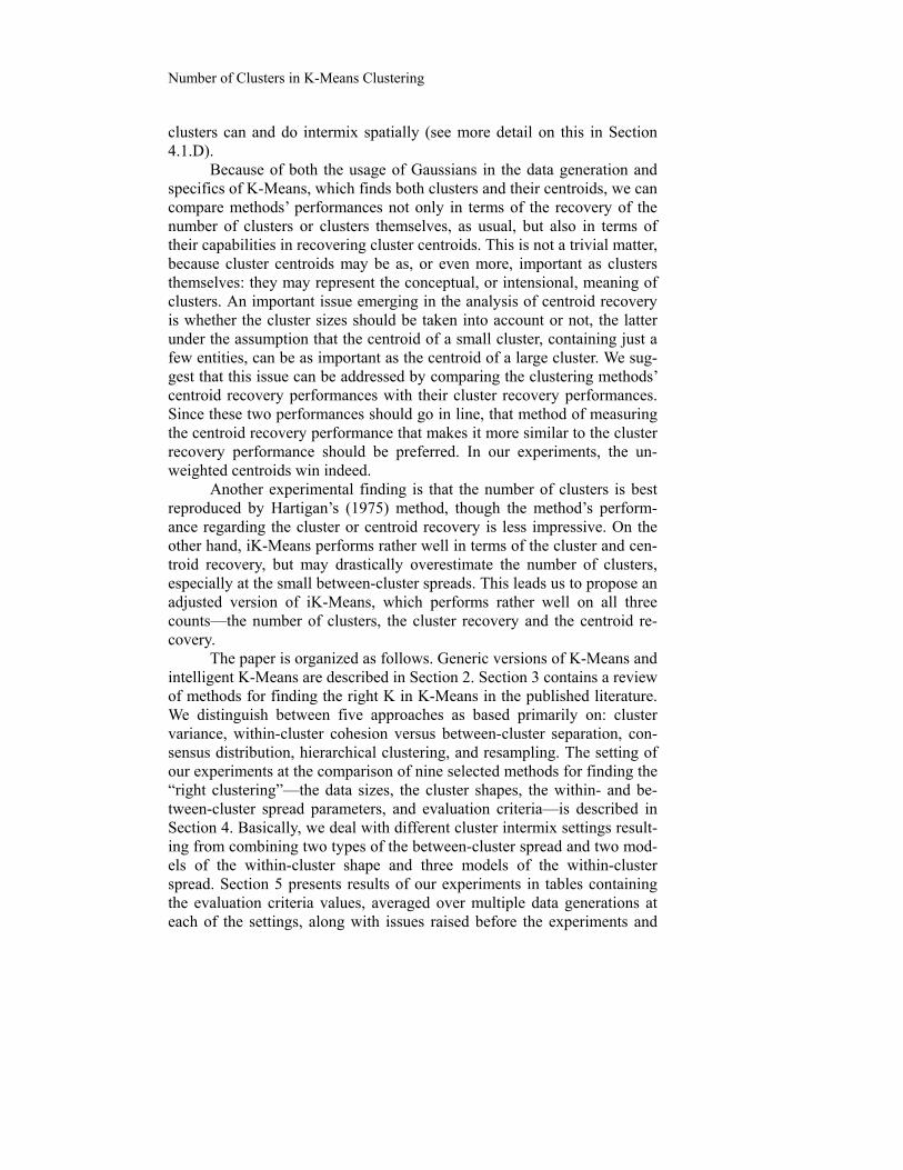
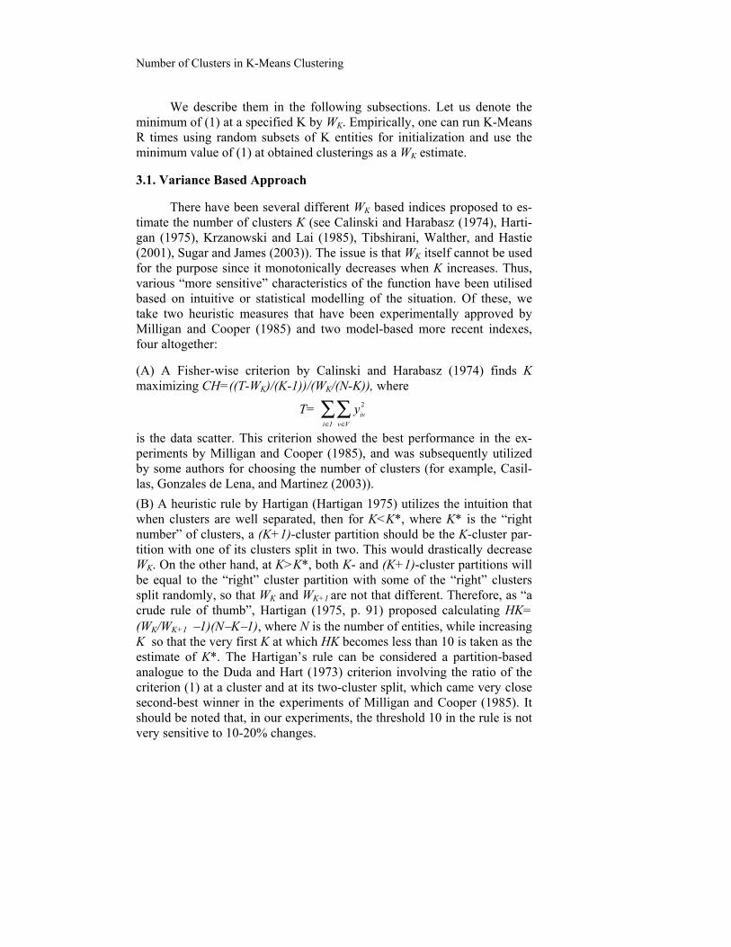
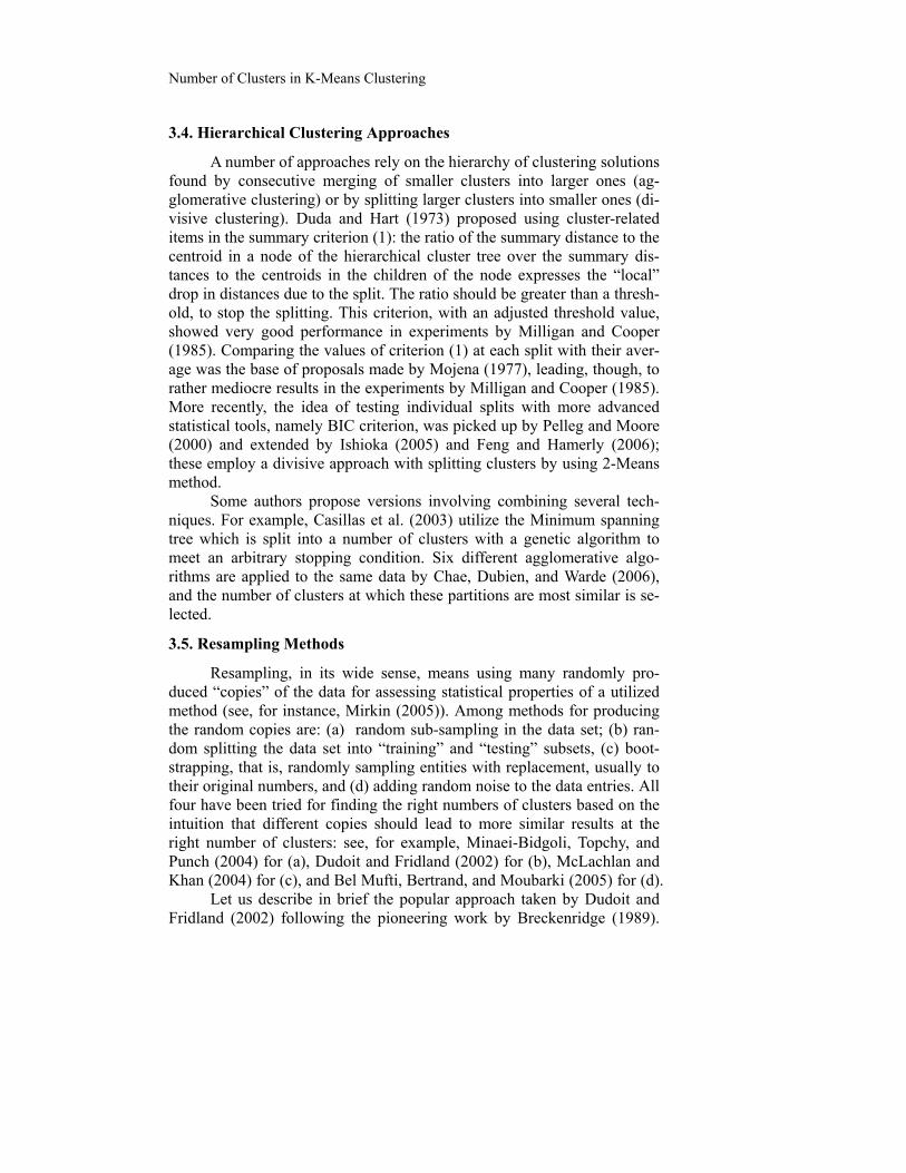
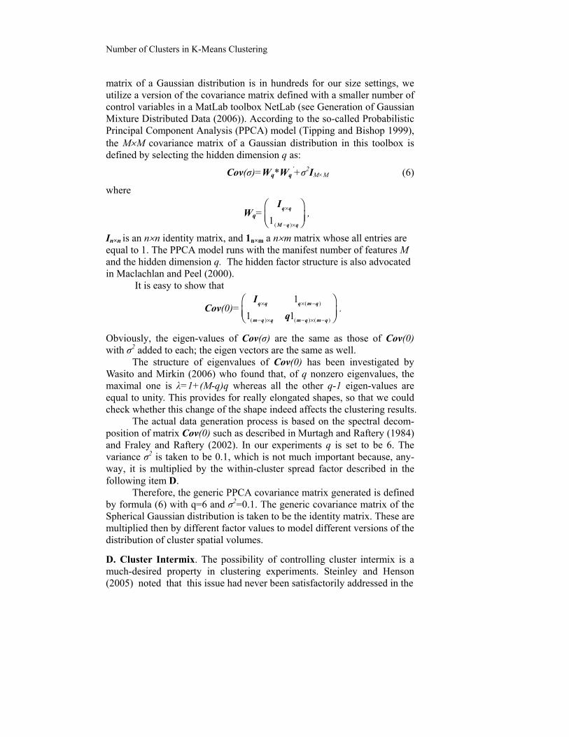
Figure 1. An illustration of the cluster intermix depending on the distance between cluster centroids (represented by pentagrams), and their covariances (represented by the indiffer-ence ellipses): two ellipses on the right are close to each other but well separated, whereas the ellipse on the left is further away but less separated because of its larger spread.
literature and proposed a mechanism for generating clusters with an ex-plicitly formalized degree of overlap, i.e. set-theoretic intersection. Spe-cifically, their model involves a value of the intersection for each pair of clusters over each single feature, thus having a disadvantage of “restricting the generation of the joint distribution clusters to be the product of the marginal distributions” (Steinley and Henson 2005, p. 245). Another prob-lem with this mechanism is by far too many parameters which are not nec-essarily directly related to parameters of the generated clusters themselves. There is also an issue of how relevant is the usage of overlapping clusters for evaluation of a partitioning method. We consider that the cluster over-lap should be modelled as the spatial intermix rather than intersection, for which parameters of distributions used for modelling individual clusters are convenient to use.
Since we utilize Gaussian clusters, their intermix is modelled by us-ing the Gaussian characteristics of location, centers, and cluster shape and spread, covariance matrices. In this way, the intermix among Gaussian clusters can be captured as a consequence of the two not necessarily re-lated aspects: the distance between cluster centroids (“between-cluster spread”) and the magnitude of their variance/covariance values (“within-cluster spread”), as illustrated on Figure 1, at which the centers of two clusters are close to each other (a small between-cluster spread) but are well separated because of small (co)variances, while another cluster, with its center being much further away, may intermix with either or both of them, because of its large (co)variances.
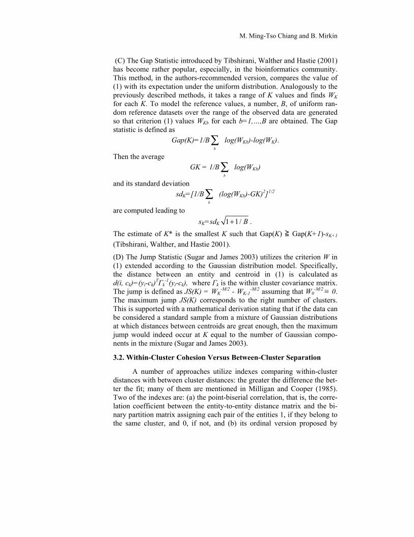
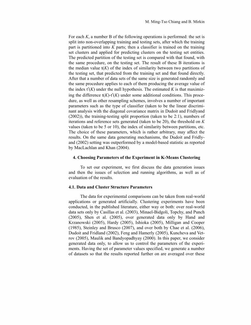
Yet Figure 1 may introduce some perception bias too, by represent-ing Gaussian clusters as ellipses. When dealing with different within-cluster variances, the perception of Gaussian clusters as being “compact” can be misleading, to an extent. Consider, for example, densities of two one-dimensional Gaussian clusters drawn on Figure 2. One, on the left, is
Number of Clusters in K-Means Clustering
−2 0 2 4 6 80
0.1
0.2
0.3
0.4
0.5
0.6
0.7
0.8
0.9
1
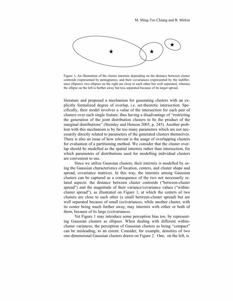
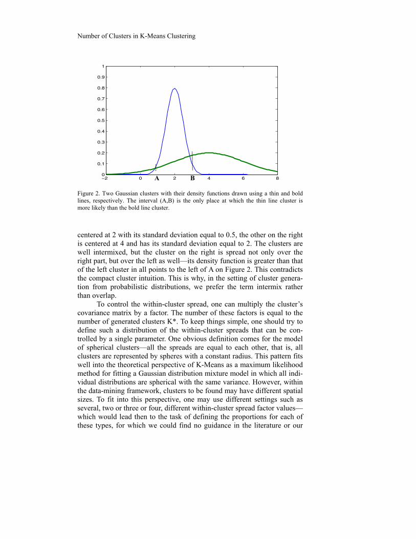
Figure 2. Two Gaussian clusters with their density functions drawn using a thin and bold lines, respectively. The interval (A,B) is the only place at which the thin line cluster is more likely than the bold line cluster.
centered at 2 with its standard deviation equal to 0.5, the other on the right is centered at 4 and has its standard deviation equal to 2. The clusters are well intermixed, but the cluster on the right is spread not only over the right part, but over the left as well—its density function is greater than that of the left cluster in all points to the left of A on Figure 2. This contradicts the compact cluster intuition. This is why, in the setting of cluster genera-tion from probabilistic distributions, we prefer the term intermix rather than overlap.
To control the within-cluster spread, one can multiply the cluster’s covariance matrix by a factor. The number of these factors is equal to the number of generated clusters K*. To keep things simple, one should try to define such a distribution of the within-cluster spreads that can be con-trolled by a single parameter. One obvious definition comes for the model of spherical clusters—all the spreads are equal to each other, that is, all clusters are represented by spheres with a constant radius. This pattern fits well into the theoretical perspective of K-Means as a maximum likelihood method for fitting a Gaussian distribution mixture model in which all indi-vidual distributions are spherical with the same variance. However, within the data-mining framework, clusters to be found may have different spatial sizes. To fit into this perspective, one may use different settings such as several, two or three or four, different within-cluster spread factor values—which would lead then to the task of defining the proportions for each of these types, for which we could find no guidance in the literature or our
A B
M. Ming-Tso Chiang and B. Mirkin
personal experiences. Therefore, we decided to go along a less challenging path by designing two types of the variant within-cluster spread factors: the “linear” and “quadratic” ones. Specifically, we take the within-cluster spread factor to be proportional to the cluster’s index k (the linear, or k-proportional distribution) or k2 (the quadratic, or k2-proportional distribu-tion), k=1, 2, …, K*. That is, with the variable within-cluster spreads, the greater the generated cluster index, the greater its spatial size. For example, the within cluster-spread of cluster 7 will be greater than the that of cluster 1, by the factor of 7 in k-proportional model and by the factor of 49 in k2-proportional model. Since the clusters are generated independently, the within-cluster spread factors can be considered as assigned to clusters ran-domly. Hence, three different models for the within-cluster spread factors utilized in our experiments are: (i) constant, (ii) k-proportional, and (iii) k2-proportional.
We maintain that an experimental clustering research may lead to conclusive results only in the case when the set of generated data struc-tures is rather narrow; inconclusive results in the published literature ap-pear when the data structures are too wide—which can be determined only after the experiment. Therefore, we are interested in keeping the set of generated data structures within a narrow range. This is why we assign, initially, a specific cluster shape with each of these models: the spherical shape for the constant spread factor (i), and the PPSA shape (6) for the k- and k2-proportional factors, (ii) and (iii). Later, in the second series of our experiments, this assignment will be relaxed to allow fully-crossed combi-nations of the chosen cluster shapes and spreads.
To control the distance between clusters with a single parameter, we utilize a special two-step mechanism for the generation of cluster locations. On the first step, all cluster centroids are generated randomly around the origin, so that each centroid entry is independently sampled from a normal distribution N(0,1) with the mean 0 and standard deviation 1. On the sec-ond step, each of these centroids is shifted away from 0, and from the oth-ers, along the line passing through the centroid and space origin, by multi-plying it with a positive factor: the greater the factor, the greater the shift, and the greater the distances between centroids.
The cluster shift factor is taken the same for all centroids. In our ex-periments, we consider two types of the between-cluster spread, “large” and “small” ones. These should be defined in such a way that the cluster-ing algorithms recover the generated clusters well at the large spreads, and less than well at the small spreads. This idea has been implemented ex-perimentally as follows: given the within-cluster spread and shape, put the between-cluster spread factor at such a value that the generated clusters are recovered on average on the level of 0.95 of the ARI index of cluster re-covery, which is defined by equation (10) below. This value is accepted
Number of Clusters in K-Means Clustering
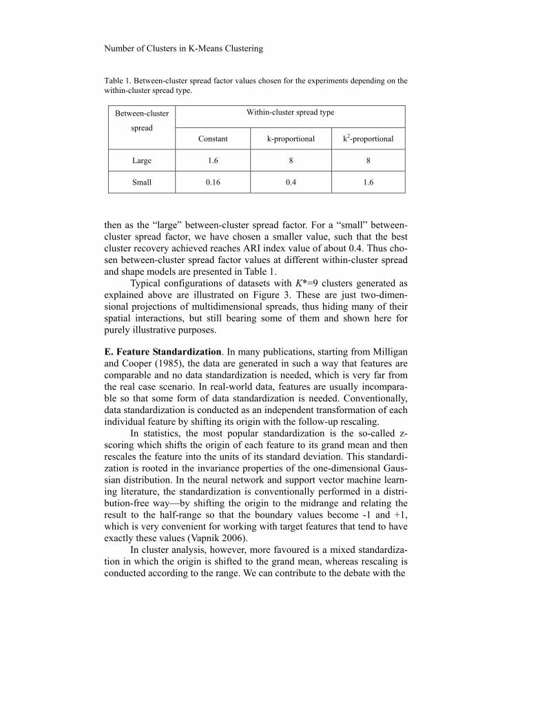
Table 1. Between-cluster spread factor values chosen for the experiments depending on the within-cluster spread type.
Between-cluster
spread
Within-cluster spread type
Constant k-proportional k2-proportional
Large 1.6 8 8
Small 0.16 0.4 1.6
then as the “large” between-cluster spread factor. For a “small” between-cluster spread factor, we have chosen a smaller value, such that the best cluster recovery achieved reaches ARI index value of about 0.4. Thus cho-sen between-cluster spread factor values at different within-cluster spread and shape models are presented in Table 1.
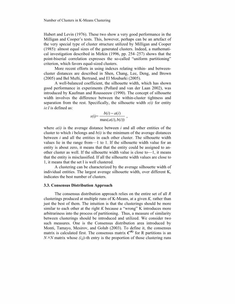
Typical configurations of datasets with K*=9 clusters generated as explained above are illustrated on Figure 3. These are just two-dimen-sional projections of multidimensional spreads, thus hiding many of their spatial interactions, but still bearing some of them and shown here for purely illustrative purposes.
E. Feature Standardization. In many publications, starting from Milligan and Cooper (1985), the data are generated in such a way that features are comparable and no data standardization is needed, which is very far from the real case scenario. In real-world data, features are usually incompara-ble so that some form of data standardization is needed. Conventionally, data standardization is conducted as an independent transformation of each individual feature by shifting its origin with the follow-up rescaling.
In statistics, the most popular standardization is the so-called z-scoring which shifts the origin of each feature to its grand mean and then rescales the feature into the units of its standard deviation. This standardi-zation is rooted in the invariance properties of the one-dimensional Gaus-sian distribution. In the neural network and support vector machine learn-ing literature, the standardization is conventionally performed in a distri-bution-free way—by shifting the origin to the midrange and relating the result to the half-range so that the boundary values become -1 and +1, which is very convenient for working with target features that tend to have exactly these values (Vapnik 2006).
In cluster analysis, however, more favoured is a mixed standardiza-tion in which the origin is shifted to the grand mean, whereas rescaling is conducted according to the range. We can contribute to the debate with the
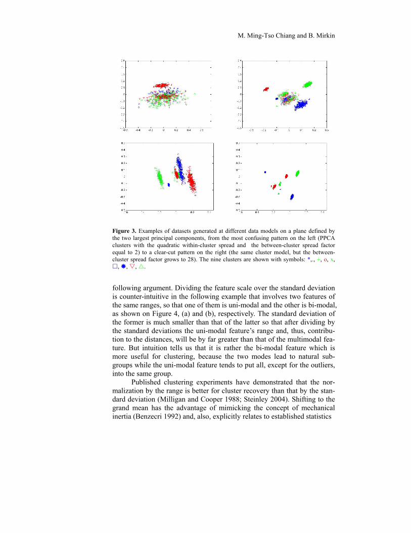
M. Ming-Tso Chiang and B. Mirkin
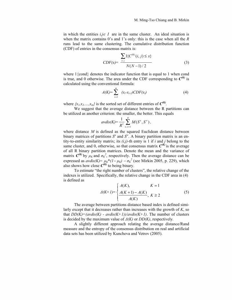
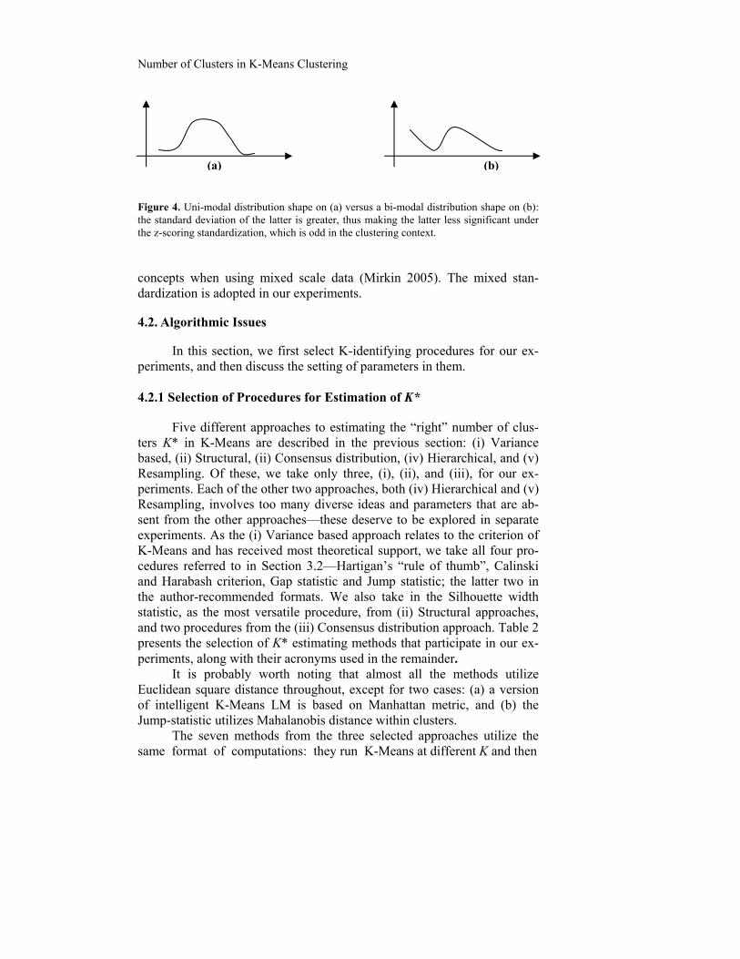
Figure 3. Examples of datasets generated at different data models on a plane defined by the two largest principal components, from the most confusing pattern on the left (PPCA clusters with the quadratic within-cluster spread and the between-cluster spread factor equal to 2) to a clear-cut pattern on the right (the same cluster model, but the between-cluster spread factor grows to 28). The nine clusters are shown with symbols: *,., +, o, x, , , , . following argument. Dividing the feature scale over the standard deviation is counter-intuitive in the following example that involves two features of the same ranges, so that one of them is uni-modal and the other is bi-modal, as shown on Figure 4, (a) and (b), respectively. The standard deviation of the former is much smaller than that of the latter so that after dividing by the standard deviations the uni-modal feature’s range and, thus, contribu-tion to the distances, will be by far greater than that of the multimodal fea-ture. But intuition tells us that it is rather the bi-modal feature which is more useful for clustering, because the two modes lead to natural sub-groups while the uni-modal feature tends to put all, except for the outliers, into the same group.
Published clustering experiments have demonstrated that the nor-malization by the range is better for cluster recovery than that by the stan-dard deviation (Milligan and Cooper 1988; Steinley 2004). Shifting to the grand mean has the advantage of mimicking the concept of mechanical inertia (Benzecri 1992) and, also, explicitly relates to established statistics
Number of Clusters in K-Means Clustering
Figure 4. Uni-modal distribution shape on (a) versus a bi-modal distribution shape on (b): the standard deviation of the latter is greater, thus making the latter less significant under the z-scoring standardization, which is odd in the clustering context.
concepts when using mixed scale data (Mirkin 2005). The mixed stan-dardization is adopted in our experiments.
4.2. Algorithmic Issues
In this section, we first select K-identifying procedures for our ex-periments, and then discuss the setting of parameters in them.
4.2.1 Selection of Procedures for Estimation of K*
Five different approaches to estimating the “right” number of clus-
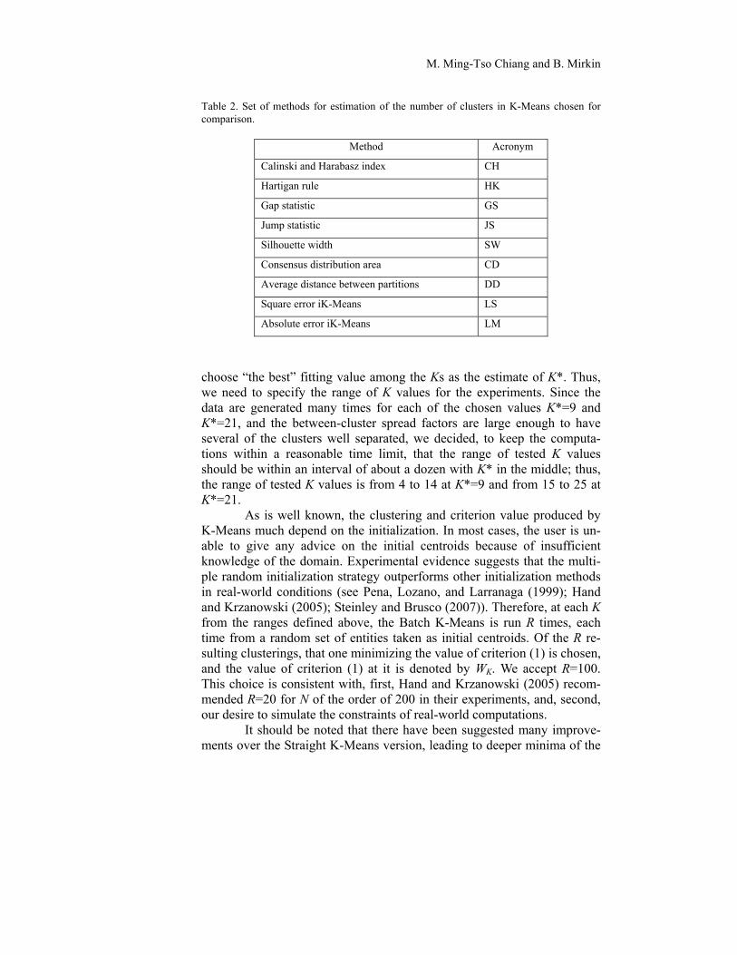
ters K* in K-Means are described in the previous section: (i) Variance based, (ii) Structural, (ii) Consensus distribution, (iv) Hierarchical, and (v) Resampling. Of these, we take only three, (i), (ii), and (iii), for our ex-periments. Each of the other two approaches, both (iv) Hierarchical and (v) Resampling, involves too many diverse ideas and parameters that are ab-sent from the other approaches—these deserve to be explored in separate experiments. As the (i) Variance based approach relates to the criterion of K-Means and has received most theoretical support, we take all four pro-cedures referred to in Section 3.2—Hartigan’s “rule of thumb”, Calinski and Harabash criterion, Gap statistic and Jump statistic; the latter two in the author-recommended formats. We also take in the Silhouette width statistic, as the most versatile procedure, from (ii) Structural approaches, and two procedures from the (iii) Consensus distribution approach. Table 2 presents the selection of K* estimating methods that participate in our ex-periments, along with their acronyms used in the remainder.
It is probably worth noting that almost all the methods utilize Euclidean square distance throughout, except for two cases: (a) a version of intelligent K-Means LM is based on Manhattan metric, and (b) the Jump-statistic utilizes Mahalanobis distance within clusters.
The seven methods from the three selected approaches utilize the same format of computations: they run K-Means at different K and then
(a) (b)
M. Ming-Tso Chiang and B. Mirkin
Table 2. Set of methods for estimation of the number of clusters in K-Means chosen for comparison.
Method Acronym
Calinski and Harabasz index CH
Hartigan rule HK
Gap statistic GS
Jump statistic JS
Silhouette width SW
Consensus distribution area CD
Average distance between partitions DD
Square error iK-Means LS
Absolute error iK-Means LM
choose “the best” fitting value among the Ks as the estimate of K*. Thus, we need to specify the range of K values for the experiments. Since the data are generated many times for each of the chosen values K*=9 and K*=21, and the between-cluster spread factors are large enough to have several of the clusters well separated, we decided, to keep the computa-tions within a reasonable time limit, that the range of tested K values should be within an interval of about a dozen with K* in the middle; thus, the range of tested K values is from 4 to 14 at K*=9 and from 15 to 25 at K*=21.
As is well known, the clustering and criterion value produced by K-Means much depend on the initialization. In most cases, the user is un-able to give any advice on the initial centroids because of insufficient knowledge of the domain. Experimental evidence suggests that the multi-ple random initialization strategy outperforms other initialization methods in real-world conditions (see Pena, Lozano, and Larranaga (1999); Hand and Krzanowski (2005); Steinley and Brusco (2007)). Therefore, at each K from the ranges defined above, the Batch K-Means is run R times, each time from a random set of entities taken as initial centroids. Of the R re-sulting clusterings, that one minimizing the value of criterion (1) is chosen, and the value of criterion (1) at it is denoted by WK. We accept R=100. This choice is consistent with, first, Hand and Krzanowski (2005) recom-mended R=20 for N of the order of 200 in their experiments, and, second, our desire to simulate the constraints of real-world computations.
It should be noted that there have been suggested many improve-ments over the Straight K-Means version, leading to deeper minima of the
Number of Clusters in K-Means Clustering
criterion (1) for the same initializations, such as the adaptable change of centroids after each entity’s Minimum distance assignment (McQueen 1967) or shifting the neighbourhoods (Hansen and Mladenovich 2001) or using simultaneously a population of solutions along with its evolutionary improvements (Maulik and Bandyopadhyay 2000, 2002; Krink and Pater-lini 2005). Different distances were explored in Leisch (2006). Modified criteria have been utilized by many (see, for reviews, Steinley (2006) and Bock (2007)). These all are left outside of our experiments: only Straight K-Means is being tested.
4.3. Evaluation Criteria
Since the generated data is a collection of entities from K* Gaussian clusters, the results of a K-Means run can be evaluated by the quality of recovery of the following components of the generated clusters: (1) the number K*, (2) the cluster centroids, and (3) the clusters themselves. This leads us to using three types of criteria based on comparison of each of these characteristics as produced by the algorithm with those in the gener-ated data. The cluster recovery conventionally is considered of greater im-portance than the other two.
The recovery of K* can be evaluated by the difference between K* and the number of clusters K in the clustering produced with a procedure under consideration. The other two are considered in the subsequent sub-sections.
4.3.1. Distance Between Centroids
Measuring the distance between found and generated centroids is
not quite straightforward even when K=K*. Some would argue that this should be done based on a one-to-one correspondence between centroids in the two sets, hence the best pair-wise distance matching between two sets. The others may consider that such a matching would not necessarily be suitable because of the asymmetry of the situation—one should care only of how well the generated centroids are reproduced by those found ones, so that if two of the found centroids are close to the same generated centroids, both should be considered its empirical representations. We ad-here to the latter view, the more so that this becomes even more relevant, both conceptually and computationally, when K differs from K*.
Another issue that should be taken into account is of the difference in cluster sizes: should the centroid of a smaller cluster bear the same weight as the centroid of a larger cluster? Or, on the contrary, should the relative cluster sizes be involved so that the smaller clusters less affect the total? To address this issue, we use both weighting schemes in the experi-
M. Ming-Tso Chiang and B. Mirkin
ments conducted, to find out which of them is more consistent with cluster recovery than the other.
According to the “asymmetric” perspective above, to score the simi-larity between the generated centroids, g1, g2, …, gK* , and those obtained using one of the chosen algorithms in Table 1, e1, e2, …, eK, we utilize a procedure consisting of the following three steps:
(a) pair-wise matching of the obtained centroids to those generated, (b) calculating distances between matching centroids, and (c) averaging the distances.
1. Pair-wise matching centroids: For each k=1,….K*, assign gk with that ej (j=1,…,K) which is the nearest to it. Any not yet assigned centroid ei then is matched to its nearest gk. 2. Computing distances: Let Ek denote the set of those ej that have been assigned to gk and αjk = qj/|Ek|, where qj is the proportion of entities in j-th found cluster (weighted version) or αjk = 1 (unweighted version). Define, for each k=1,…,K, dis(k) = ejEk d(gk,ej)* αjk . The weighted distance is the average weighted distance between the generated and the set of match-ing centroids in the computed clusters; the unweighted distance is just the summary distance between all matching pairs of clusters. (The distance d here is Euclidean squared distance.)
3. Averaging distances: Calculate D=
*
1
)(*K
kk kdisp where pk=Nk= |Sk|,
is the number of entities in the generated k-th cluster (in the weighted ver-sion), or pk= 1/K* (in the unweighted version).
4.3.2 Confusion Between Partitions
To measure similarity between two partitions, the contingency (con-
fusion) table is used. Entries in the contingency table are the co-occurrence frequencies of the generated partition clusters (row categories) and the ob-tained clusters (column categories): they are the counts of entities that fall simultaneously in both. Denote the generated clusters (rows) by k, the ob-tained partition clusters (columns) by j and the co-occurrence counts by Nkj. The frequencies of row and column categories (cluster sizes) are de-noted by Nk+ and N+j. The relative frequencies are defined accordingly as pkj=Nkj/N, pk+=Nk+/N, and p+j=N+j/N, where N is the total number of enti-ties. We use a conventional similarity measure, the adjusted Rand index ARI defined by the following formula (Hubert and Arabie 1985; Yeung and Ruzzo 2001):
Number of Clusters in K-Means Clustering
2/
22222
1
2/
222
1111
111 1
NNNNN
NNNN
ARIL
l
lK
k
kL
l
lK
k
k
L
l
lK
k
kK
k
L
l
kl
where
2
)1(2
NNN
.
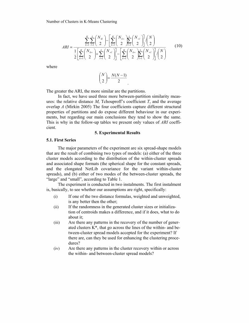
The greater the ARI, the more similar are the partitions. In fact, we have used three more between-partition similarity meas-
ures: the relative distance M, Tchouproff’s coefficient T, and the average overlap A (Mirkin 2005) The four coefficients capture different structural properties of partitions and do expose different behaviour in our experi-ments, but regarding our main conclusions they tend to show the same. This is why in the follow-up tables we present only values of ARI coeffi-cient.
5. Experimental Results
5.1. First Series
The major parameters of the experiment are six spread-shape models that are the result of combining two types of models: (a) either of the three cluster models according to the distribution of the within-cluster spreads and associated shape formats (the spherical shape for the constant spreads, and the elongated NetLib covariance for the variant within-cluster spreads), and (b) either of two modes of the between-cluster spreads, the “large” and “small”, according to Table 1.
The experiment is conducted in two instalments. The first instalment is, basically, to see whether our assumptions are right, specifically:
(i) If one of the two distance formulas, weighted and unweighted, is any better then the other;
(ii) If the randomness in the generated cluster sizes or initializa-tion of centroids makes a difference, and if it does, what to do about it;
(iii) Are there any patterns in the recovery of the number of gener-ated clusters K*, that go across the lines of the within- and be-tween-cluster spread models accepted for the experiment? If there are, can they be used for enhancing the clustering proce-dures?
(iv) Are there any patterns in the cluster recovery within or across the within- and between-cluster spread models?
(10)
M. Ming-Tso Chiang and B. Mirkin
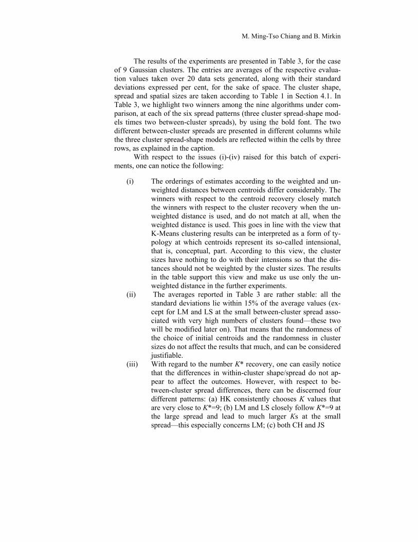
The results of the experiments are presented in Table 3, for the case of 9 Gaussian clusters. The entries are averages of the respective evalua-tion values taken over 20 data sets generated, along with their standard deviations expressed per cent, for the sake of space. The cluster shape, spread and spatial sizes are taken according to Table 1 in Section 4.1. In Table 3, we highlight two winners among the nine algorithms under com-parison, at each of the six spread patterns (three cluster spread-shape mod-els times two between-cluster spreads), by using the bold font. The two different between-cluster spreads are presented in different columns while the three cluster spread-shape models are reflected within the cells by three rows, as explained in the caption.
With respect to the issues (i)-(iv) raised for this batch of experi-ments, one can notice the following:
(i) The orderings of estimates according to the weighted and un-
weighted distances between centroids differ considerably. The winners with respect to the centroid recovery closely match the winners with respect to the cluster recovery when the un-weighted distance is used, and do not match at all, when the weighted distance is used. This goes in line with the view that K-Means clustering results can be interpreted as a form of ty-pology at which centroids represent its so-called intensional, that is, conceptual, part. According to this view, the cluster sizes have nothing to do with their intensions so that the dis-tances should not be weighted by the cluster sizes. The results in the table support this view and make us use only the un-weighted distance in the further experiments.
(ii) The averages reported in Table 3 are rather stable: all the standard deviations lie within 15% of the average values (ex-cept for LM and LS at the small between-cluster spread asso-ciated with very high numbers of clusters found—these two will be modified later on). That means that the randomness of the choice of initial centroids and the randomness in cluster sizes do not affect the results that much, and can be considered justifiable.
(iii) With regard to the number K* recovery, one can easily notice that the differences in within-cluster shape/spread do not ap-pear to affect the outcomes. However, with respect to be-tween-cluster spread differences, there can be discerned four different patterns: (a) HK consistently chooses K values that are very close to K*=9; (b) LM and LS closely follow K*=9 at the large spread and lead to much larger Ks at the small spread—this especially concerns LM; (c) both CH and JS
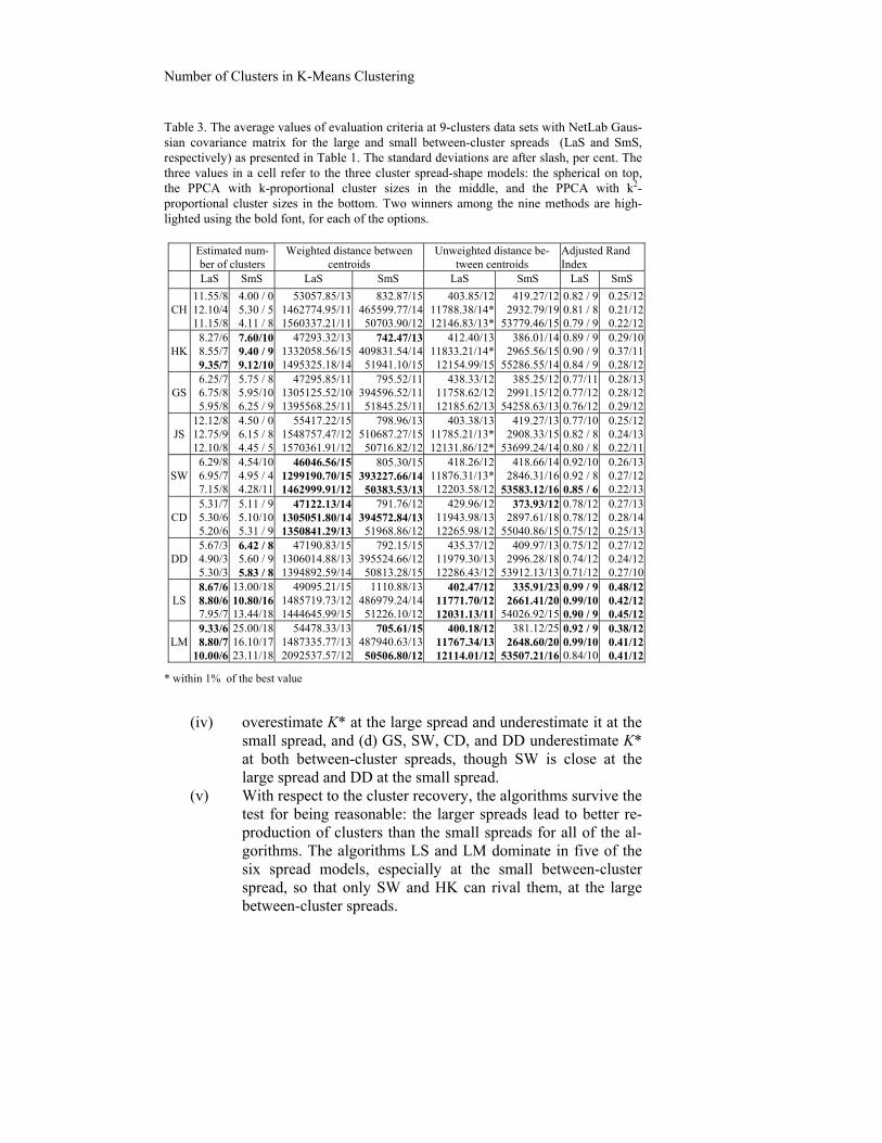
Number of Clusters in K-Means Clustering
Table 3. The average values of evaluation criteria at 9-clusters data sets with NetLab Gaus-sian covariance matrix for the large and small between-cluster spreads (LaS and SmS, respectively) as presented in Table 1. The standard deviations are after slash, per cent. The three values in a cell refer to the three cluster spread-shape models: the spherical on top, the PPCA with k-proportional cluster sizes in the middle, and the PPCA with k2-proportional cluster sizes in the bottom. Two winners among the nine methods are high-lighted using the bold font, for each of the options. Estimated num-
ber of clustersWeighted distance between
centroidsUnweighted distance be-
tween centroidsAdjusted Rand Index
LaS SmS LaS SmS LaS SmS LaS SmS
CH 11.55/8 12.10/4 11.15/8
4.00 / 0 5.30 / 5 4.11 / 8
53057.85/13 1462774.95/11 1560337.21/11
832.87/15465599.77/14
50703.90/12
403.85/1211788.38/14*12146.83/13*
419.27/122932.79/19
53779.46/15
0.82 / 90.81 / 80.79 / 9
0.25/12 0.21/12 0.22/12
HK 8.27/6 8.55/7 9.35/7
7.60/10 9.40 / 9 9.12/10
47293.32/13 1332058.56/15 1495325.18/14
742.47/13409831.54/14
51941.10/15
412.40/1311833.21/14*
12154.99/15
386.01/142965.56/15
55286.55/14
0.89 / 90.90 / 90.84 / 9
0.29/10 0.37/11 0.28/12
GS 6.25/7 6.75/8 5.95/8
5.75 / 8 5.95/10 6.25 / 9
47295.85/11 1305125.52/10 1395568.25/11
795.52/11394596.52/11
51845.25/11
438.33/1211758.62/1212185.62/13
385.25/122991.15/12
54258.63/13
0.77/110.77/120.76/12
0.28/13 0.28/12 0.29/12
JS 12.12/8 12.75/9 12.10/8
4.50 / 0 6.15 / 8 4.45 / 5
55417.22/15 1548757.47/12 1570361.91/12
798.96/13510687.27/15
50716.82/12
403.38/1311785.21/13*12131.86/12*
419.27/132908.33/15
53699.24/14
0.77/100.82 / 80.80 / 8
0.25/12 0.24/13 0.22/11
SW 6.29/8 6.95/7 7.15/8
4.54/10 4.95 / 4 4.28/11
46046.56/15 1299190.70/15 1462999.91/12
805.30/15393227.66/14
50383.53/13
418.26/1211876.31/13*
12203.58/12
418.66/142846.31/16
53583.12/16
0.92/100.92 / 80.85 / 6
0.26/13 0.27/12 0.22/13
CD 5.31/7 5.30/6 5.20/6
5.11 / 9 5.10/10 5.31 / 9
47122.13/14 1305051.80/14 1350841.29/13
791.76/12394572.84/13
51968.86/12
429.96/1211943.98/1312265.98/12
373.93/122897.61/18
55040.86/15
0.78/120.78/120.75/12
0.27/13 0.28/14 0.25/13
DD 5.67/3 4.90/3 5.30/3
6.42 / 8 5.60 / 9 5.83 / 8
47190.83/15 1306014.88/13 1394892.59/14
792.15/15395524.66/12
50813.28/15
435.37/1211979.30/1312286.43/12
409.97/132996.28/18
53912.13/13
0.75/120.74/120.71/12
0.27/12 0.24/12 0.27/10
LS 8.67/6 8.80/6 7.95/7
13.00/18 10.80/16 13.44/18
49095.21/15 1485719.73/12 1444645.99/15
1110.88/13486979.24/14
51226.10/12
402.47/1211771.70/1212031.13/11
335.91/232661.41/20
54026.92/15
0.99 / 90.99/100.90 / 9
0.48/12 0.42/12 0.45/12
LM 9.33/6 8.80/7
10.00/6
25.00/18 16.10/17 23.11/18
54478.33/13 1487335.77/13 2092537.57/12
705.61/15487940.63/13
50506.80/12
400.18/1211767.34/1312114.01/12
381.12/252648.60/20
53507.21/16
0.92 / 90.99/100.84/10
0.38/12 0.41/12 0.41/12
* within 1% of the best value
(iv) overestimate K* at the large spread and underestimate it at the
small spread, and (d) GS, SW, CD, and DD underestimate K* at both between-cluster spreads, though SW is close at the large spread and DD at the small spread.
(v) With respect to the cluster recovery, the algorithms survive the test for being reasonable: the larger spreads lead to better re-production of clusters than the small spreads for all of the al-gorithms. The algorithms LS and LM dominate in five of the six spread models, especially at the small between-cluster spread, so that only SW and HK can rival them, at the large between-cluster spreads.
M. Ming-Tso Chiang and B. Mirkin
5.2 HK-Adjustment of the iK-Means
According to the experiment, iK-Means methods LS and LM may lead to excessive numbers of clusters, while HK, on the other hand, makes a very good recovery of the number of clusters. This leads us to suggest that the HK number-of-cluster results should be taken as a reference to adjust the threshold for removing small AP clusters for the initial setting in iK-Means. So far, only AP singletons are removed from the initial setting. If other “smaller” AP clusters are removed, the chosen K will be smaller and, thus, closer to K*. A straightforward option would just remove all AP clusters whose sizes are less than or equal to a pre-specified discarding threshold D. Given Kh, found with the Hartigan rule, a suitable discarding threshold D can be found in such a way that the number of clusters KD identified with D, taken as the discarding threshold, is close enough to Kh. This can be done by gradually increasing D from the default value D=1. A typical sequence of steps, at a given Kh, say Kh =9, could be like this: at D=1, the number of AP clusters is KD =32; at D=2, still KD =32, that is, no doubletons among the AP clusters; then K3 =29, K4 =24, K8 =20, K11 =14, K12 =11, and K14 =8 (the omitted D values give no reduction in KD values). Therefore, D should be taken as D=14. Since Kh value is not necessarily correct but rather indicative, D=12, leading to 11 clusters, is also accept-able, especially if K*=10 or 11. Thus, one can use a computational routine of increasing D one by one until KD becomes less than Kh. When we put =1.1, the next KD value is typically less than Kh, whereas =1.2 leaves KD rather large, but =1.15 produces reasonable approximations of Kh. We refer to thus HK conditioned versions of LS and LM as ALS and ALM.
5.3 Second Experimental Series
The second series of our experiments differs from the first one in
three aspects:
(1) The adjusted versions of iK-Means clustering, ALS and ALM, are in-cluded in the list of methods; (2) Data sets with the number of clusters K* in two versions, 9 and 21 clusters, are generated as described in Section 4.1; (3) The cluster shapes and cluster distances are fully crossed now. Therefore, the set of data structures generated here is expanded to 24 mod-els by fully crossing the following four factors:
(a) Two versions of the number of clusters K*, 9 and 21 clusters;
Number of Clusters in K-Means Clustering
(b) Two versions of the cluster shape, either spherical or elliptical, as described in Section 4.1.C;
(c) Three versions of the within-cluster spread—constant, linear and quadratic, as described in Section 4.1.D;
(d) Two versions of the between-cluster spread, large and small, as described in Section 4.1.D with the spread factor values presented in Table 1.
The issues to be addressed in these experiments are those (ii)-(iv) above, and, additionally, as follows:
(vi) Is there any pattern of (dis)similarity between the two data size formats;
(vii) Are the HK-adjusted iK-Means methods better than the origi-nal ones;
(viii) Are the algorithms’ recovery properties at the constant spheri-cal within-cluster-spread model any better than those at the elongated not-constant spread clusters?
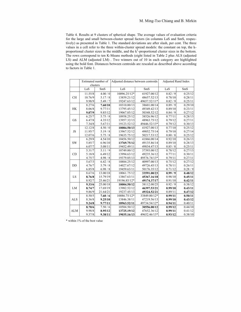
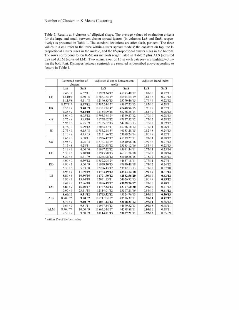
The averaged, over ten to twenty data sets generated at each of the 24 pat-terns, evaluation criteria values are presented in Tables 4 to 7. Each of the four tables corresponds to one of the four combinations of the size (a) and shape (b) factors, whereas the six combinations of factors (c) and (d) are presented within each of the Tables 4 – 7.
The cluster centroid recovery results in Tables 4 – 7 are presented with a change in reporting: the weighted distance case is removed so that only the unweighted distances are left. Moreover, the distances are re-scaled to achieve comparability across the between-cluster spread models, so that issue (viii) can be addressed with just visual inspection by a naked eye. The rescaling is conducted according to the inter-cluster spread factor values in Table 1 and takes into account that, at the small within-cluster spreads, the spread factor value at k2-proportional model, 2, is four times greater than that at k-proportional model, 0.5, and 10 times greater than that at the equal spread model, 0.2. By multiplying the distances between centroids at the equal spread model by 100=102 and at the k-proportional model by 16=42, they are made comparable with those at the k2-proportional model. (Note that the distance between centroids is squared Euclidean, which implies the quadratic adjustment of the factors.) Simi-larly, at the large spreads, the within-cluster spread factors at the variant spread models are the same while that at the constant spread model is 5 times smaller. Multiplying the distances between centroids at the equal spread model by 25 makes all the distances in the Tables comparable.
M. Ming-Tso Chiang and B. Mirkin
Table 4. Results at 9 clusters of spherical shape. The average values of evaluation criteria for the large and small between-cluster spread factors (in columns LaS and SmS, respec-tively) as presented in Table 1. The standard deviations are after slash, per cent. The three values in a cell refer to the three within-cluster spread models: the constant on top, the k-proportional cluster sizes in the middle, and the k2-proportional cluster sizes in the bottom. The rows correspond to ten K-Means methods (eight listed in Table 2 plus ALS (adjusted LS) and ALM (adjusted LM) . Two winners out of 10 in each category are highlighted using the bold font. Distances between centroids are rescaled as described above according to factors in Table 1.
Estimated number of clusters
Adjusted distance between centroids Adjusted Rand Index
LaS SmS LaS SmS LaS SmS
CH 11.55/8 10.76/9
9.98/9
4.00 / 05.17 / 85.49 / 7
10096.25/12*13859.21/1219247.63/12
41927.00/1248657.52/13
49657.52/11*
0.82 / 9 0.78/10 0.82 / 9
0.25/12 0.28/11 0.25/11
HK 8.27/6 8.06/8 9.07/9
7.60/109.77/119.85/12
10310.00/1313795.45/1219067.85/12
38601.00/1449349.42/1350348.52/12
0.89 / 9 0.89/10 0.84 / 9
0.29/10 0.23/11 0.27/12
GS 6.25/7 6.47/8 7.34/8
5.75 / 84.35/125.67/11
10958.25/1213957.32/1319123.52/12
38526.96/1248963.75/12
49446.52/13*
0.77/11 0.79/12 0.79/12
0.28/13 0.27/11 0.30/13
JS 12.12/8 11.95/7 12.07/6
4.50 / 05.19 / 85.75 / 8
10084.50/1313967.52/1219635.75/12
41927.00/1349052.75/1450217.53/12
0.77/10 0.79/10 0.80 / 8
0.25/12 0.27/14 0.25/12
SW 6.29/8 5.85/7 6.07/7
4.54/106.96/105.08/11
10456.50/1213769.75/1219452.49/11
41866.00/1449135.86/1449834.47/13
0.92/10 0.89/10 0.85 / 8
0.26/13 0.28/13 0.25/11
CD 5.31/7 5.18/8 4.75/7
5.11 / 96.49/124.98 / 8
10749.00/1213994.63/1219379.85/13
37393.00/1249235.36/12
49576.74/13*
0.78/12 0.77/11 0.79/11
0.27/13 0.30/11 0.27/11
DD 5.67/3 4.76/7 6.85/8
6.42 / 85.79 / 86.98 / 8
10884.25/1214027.67/1219459.63/11
40997.00/1349726.45/1350176.35/12
0.75/12 0.78/11 0.71/12
0.27/12 0.26/11 0.28 / 9
LS 8.67/6 8.76/8 8.92/7
13.00/1815.79/1925.46/21
10061.75/1213867.63/11
19196.85/12*
33591.00/2345367.16/1849174.37/17
0.99 / 9 0.98/10 0.91/10
0.48/12 0.45/11 0.42/11
LM 9.33/6 8.74/7 9.86/9
25.00/1817.69/1921.64/21
10004.50/1213982.52/1219237.45/13
38112.00/2546397.53/2149324.52/21
0.92 / 9 0.99/10 0.89/11
0.38/12 0.43/11 0.47/12
ALS 8.50/5 8.36/8 9.24/8
7.60 / 69.25/109.77/11
10086.75/12*13846.38/1118963.52/11
33849.00/12*47219.56/13
49734.54/12*
0.99/11 0.99/10 0.94/11
0.50/11 0.43/12 0.40/11
ALM 8.70/6 9.98/8 9.37/8
7.50 / 68.95/129.38/11
10504.50/1213725.19/1219035.16/13
30556.00/1247652.36/12
49652.46/13*
0.99/12 0.99/11 0.93/12
0.44/10 0.41/12 0.38/10
* within 1% of the best value
Number of Clusters in K-Means Clustering
Table 5. Results at 9 clusters of elliptical shape. The average values of evaluation criteria for the large and small between-cluster spread factors (in columns LaS and SmS, respec-tively) as presented in Table 1. The standard deviations are after slash, per cent. The three values in a cell refer to the three within-cluster spread models: the constant on top, the k-proportional cluster sizes in the middle, and the k2-proportional cluster sizes in the bottom. The rows correspond to ten K-Means methods (eight listed in Table 2 plus ALS (adjusted LS) and ALM (adjusted LM). Two winners out of 10 in each category are highlighted us-ing the bold font. Distances between centroids are rescaled as described above according to factors in Table 1.
Estimated number of clusters
Adjusted distance between cen-troids
Adjusted Rand Index
LaS SmS LaS SmS LaS SmS
CH 9.43/12 12.10/4 11.15/8
6.52/11 5.30 / 5 4.11 / 8
11969.34/12 11788.38/14*
12146.83/13
45793.48/12 46924.64/19 53779.46/15
0.81/100.81 / 80.79 / 9
0.27/11 0.21/12 0.22/12
HK 8.57/11*
8.55 / 7 9.35 / 7
8.97/12 9.40 / 9 9.12/10
11785.34/12* 11833.21/14*
12154.99/15
43967.25/1347448.96/15 55286.55/14
0.85/100.90 / 90.84 / 9
0.28/11 0.37/11 0.28/12
GS 5.00 / 0 6.75 / 8 5.95 / 8
6.95/12 5.95/10 6.25 / 9
11795.36/12* 11758.62/12 12185.62/13
44369.27/12 47857.52/12 54258.63/13
0.79/10 0.77/12 0.76/12
0.28/13 0.28/12 0.29/12
JS 11.75/10 12.75 / 9 12.10 / 8
5.29/12 6.15 / 8 4.45 / 5
12084.37/11 11785.21/13*
12131.86/12
45736.18/12 46533.28/15 53699.24/14
0.77/11 0.82 / 80.80 / 8
0.26/11 0.24/13 0.22/11
SW 7.65 / 9 6.95 / 7 7.15 / 8
5.08/11 4.95 / 4 4.28/11
11936.47/12 11876.31/13*
12203.58/12
45739.27/11 45540.96/16 53583.12/16
0.91/110.92 / 80.85 / 6
0.28/12 0.27/12 0.22/13
CD 5.19 / 9 5.30 / 6 5.20 / 6
4.00 / 0 5.10/10 5.31 / 9
11997.52/12 11943.98/13 12265.98/12
45691.34/11 46361.76/18 55040.86/15
0.77/110.78/120.75/12
0.25/14 0.28/14 0.25/13
DD 4.00 / 0 4.90 / 3 5.30 / 3
6.39/12 5.60 / 9 5.83 / 8
11857.20/12* 11979.30/13 12286.43/12
44637.18/11 47940.48/18 53912.13/13
0.77/110.74/120.71/12
0.27/11 0.24/12 0.27/10
LS 8.95 / 9 8.80 / 6 7.95 / 7
11.69/19 10.80/16 13.44/18
11753.19/12 11771.70/12 12031.13/11
43593.14/18 42582.56/20 54026.92/15
0.99 / 90.99/100.90 / 9
0.51/13 0.42/12 0.45/12
LM 8.47 / 9 8.80 / 7
10.00 / 6
17.96/18 16.10/17 23.11/18
11896.49/12 11767.34/13 12114.01/12
43829.76/17 42377.60/20 53507.21/16
0.91/100.99/100.84/10
0.40/11 0.41/12 0.41/12
ALS 8.69/10
8.70 / 7* 8.70 / 9
9.31/12 9.90 / 7 9.40 / 9
11763.52/12 11871.70/15*
11031.13/12
45324.76/13 43536.32/11 52098.21/12
0.99/10 0.99/11 0.95/11
0.50/13 0.42/12 0.38/12
ALM 9.64 / 9
8.70 / 7* 9.50 / 9
9.81/11 10.60 / 9
9.60 / 9
11967.54/13 11867.34/15*
10114.01/13
44679.52/13 44298.88/11 53057.21/11
0.99/13 0.99/10 0.92/13
0.48/11 0.38/11 0.35 / 9
* within 1% of the best value

M. Ming-Tso Chiang and B. Mirkin
Table 6. Results at 21 clusters of spherical shape. The average values of evaluation criteria for the large and small between-cluster spread factors (in columns LaS and SmS, respec-tively) as presented in Table 1. The standard deviations are after slash, per cent. The three values in a cell refer to the three within-cluster spread models: the constant on top, the k-proportional cluster sizes in the middle, and the k2-proportional cluster sizes in the bottom. The rows correspond to ten K-Means methods (eight listed in Table 2 plus ALS (adjusted LS) and ALM (adjusted LM). Two winners out of ten in each category are highlighted using the bold font. Distances between centroids are rescaled as described above according to factors in Table 1.
Estimated number of clusters
Adjusted distance between cen-troids
Adjusted Rand Index
LaS SmS LaS SmS LaS SmS
CH 24.56 / 9 23.49/11 24.63 / 9
15.00 / 0 16.83 / 8 17.09/10
14598.62/10*16658.37/1319254.52/12
24583.26/10 25869.74/13 28563.64/13
0.79 / 8 0.82 / 9 0.79 / 9
0.24/11 0.28/12 0.25/12
HK 20.45/8
20.95 / 8 22.85 / 7
18.50 / 8 20.39/10 22.79/10
14378.52/11*16764.96/1319246.34/13
26164.25/1326946.37/13 28837.96/13
0.90 / 9 0.88/11 0.88/10
0.21/11 0.39/12 0.30/12
GS 18.32 / 9 18.75/10 18.19/11
15.32/1017.91/1018.04/10
15489.65/1016431.05/13
19113452/13
24354.25/1125736.48/1328543.65/13
0.81/11 0.81/11 0.78/11
0.25/11 0.26/12 0.29/11
JS 25.58 / 7 23.27 / 8 24.08/11
15.00 / 0 17.63 / 9 16.74 / 8
14478.96/12*16776.14/1219248.52/13
24583.26/10 25960.81/13 28619.57/11
0.76/10 0.83 / 8 0.82/10
0.24/11 0.27/13 0.25/11
SW 19.35 / 8 17.87/10 18.65 / 8
17.50/10 17.38 / 8 18.29 / 9
15895.52/1116737.57/1319376.19/11
22267.25/12* 25842.51/13 28736.11/13
0.93/10 0.90/10 0.83 / 8
0.26/12 0.28/11 0.25/12
CD 17.52 / 9 18.17 / 7 17.51 / 9
17.00 / 0 17.82 / 9 18.07/10
15254.95/1116493.24/1319237.82/13
27154.26/12 25964.75/13 28893.12/14
0.79/12 0.78/11 0.77/10
0.30/11 0.29/12 0.31/13
DD 17.84 / 9 16.38 / 8 17.74/10
17.25 / 8 17.64/10 18.19/12
15269.52/1116793.52/13 19436.42/11
26458.25/10 26019.57/13 28631.75/13
0.79/12 0.74/10 0.70/11
0.35/11 0.29/12 0.31/10
LS 20.85 / 7 21.43 / 8 20.74 / 9
25.85 / 8 29.42/12 31.48/15
14254.85/1116237.10/1318934.26/13
26954.23/12 25234.27/13 28443.59/13
0.99 / 9 0.98/10*
0.94/10
0.36/10 0.46/12 0.41/12
LM 21.56/8
21.96/10 22.16/10
37.45/18 34.63/17 39.67/19
15254.85/1116634.91/1318896.17/13
24586.23/12 25336.52/19 28651.63/16
0.96 / 9* 0.99/10 0.90/11
0.40/11 0.43/11*
0.39/11
ALS 20.32/8 21.76/9
21.87 / 9
19.85 / 6 20.79 / 7 22.10 / 9
14358.95/1116349.27/1319234.71/12
22145.85/10 25729.15/13 28931.25/10
0.99/11 0.99/11 0.98/11
0.50/11 0.45/11
0.37/12*
ALM
21.25 / 9 21.07 / 9 22.13 / 8
22.52 / 6 22.61/10 21.63 / 8
15254.95/1116836.49/1219273.85/13
21856.32/12 26167.29/13 28392.24/11
0.99/12 0.99/11 0.95/12
0.45/11 0.39/11
0.36/10*
* within 1% of the best value
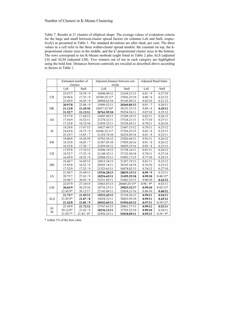
Number of Clusters in K-Means Clustering
Table 7. Results at 21 clusters of elliptical shape. The average values of evaluation criteria for the large and small between-cluster spread factors (in columns LaS and SmS, respec-tively) as presented in Table 1. The standard deviations are after slash, per cent. The three values in a cell refer to the three within-cluster spread models: the constant on top, the k-proportional cluster sizes in the middle, and the k2-proportional cluster sizes in the bottom. The rows correspond to ten K-Means methods (eight listed in Table 2 plus ALS (adjusted LS) and ALM (adjusted LM). Two winners out of ten in each category are highlighted using the bold font. Distances between centroids are rescaled as described above according to factors in Table 1.
Estimated number of
clusters Adjusted distance between cen-
troidsAdjusted Rand Index
LaS SmS LaS SmS LaS SmS
CH 25.67/7 24.96/8 23.45/9
18.59 / 9 17.35 / 9 16.45 / 9
16948.49/1218789.25/11*
20984.62/10
21654.51/13 37856.25/19 55145.89/12
0.81 / 90.80 / 80.82/10
0.27/10 0.23/12 0.21/12
HK 20.97/8 21.12/8 21.52/7
22.08 / 9 21.45/10 21.12/11
15949.52/1118457.52/10*
20761.95/10
20369.85/1338152.52/15 59254.56/11
0.91 / 70.89 / 80.87/10
0.20/11 0.45/12 0.35/12
GS 19.57/8 17.56/9 17.52/8
17.64/12 16.52/11 18.32/10
16495.49/1321278.32/1121859.32/11
21549.18/1337524.21/1155328.45/11
0.82/110.77/100.79/11
0.26/120.27/110.26/10
JS 19.24/8 24.65/8 25.25/7
17.67/13 18.75 / 9 15.85 / 7
16627.49/1318546.32/11*
21254.74/10
21687.13/12 37526.25/15 56254.85/14
0.78/11 0.82 / 80.81 / 9
0.23/12 0.25/13 0.25/11
SW 18.00/0 18.35/8 18.52/8
18.26/10 16.85 / 7 17.38 / 7
16762.56/1221587.85/1022459.45/12
21026.84/13 37859.26/16 56859.25/16
0.91/110.91 / 80.85 / 8
0.26/12 0.26/12 0.23/13
CD 17.97/8 18.52/7 16.45/9
17.32/13 17.25 / 8 18.52 / 9
16596.19/1321148.52/1122984.52/11
21738.16/11 37152.56/18 55492.17/15
0.81/110.78/110.77/10
0.26/12 0.27/14 0.29/13
DD 18.46/7 15.95/8 17.52/9
16.85/12 16.52 / 9 17.25 / 9
16815.24/1320365.14/11 21523.65/11
21267.19/13 38185.54/18 56874.82/13
0.81/110.76/100.76/12
0.33/12 0.25/12 0.27/10
LS 21.96/7 20.75/7 18.96/7
25.49/13 27.65 / 9 30.45 / 9
15536.28/1318254.65/1122351.85/11
20035.15/13 31459.25/18 53462.52/15
0.99 / 90.99/100.90/10
0.33/11 0.40/12*
0.42/12
LM 22.07/9 20.65/9
22.45/9*
27.10/15 36.25/16 38.12/17
15863.87/1318754.25/1122145.88/11
20469.25/15* 29025.52/17 52854.21/16
0.98 / 9*0.99/100.86/10
0.43/11 0.42/12*
0.40/12
ALS 21.72/7
21.85/9* 21.42/8
21.95/13 21.87 / 8 21.85 / 9
15532.45/1219658.52/1120542.65/11
21354.56/13 38452.95/10 51954.65/12
0.99/11 0.99/11 0.97/11
0.54/11 0.45/12
0.39/12*
ALM
22.49/9 20.12/8* 21.85/7*
21.72/12 23.45 / 9
21.45 / 8*
15767.63/1318236.12/1122956.25/11
20861.57/13 37529.52/10 52018.85/11
0.99/12 0.99/10 0.95/13
0.52/11 0.38/11
0.38 / 9*
* within 1% of the best value
M. Ming-Tso Chiang and B. Mirkin
Here are the findings related to each of the issues above:
(v) Tables 4 to 7 show a remarkable degree of similarity regarding the main findings of the first series of experiments: a. The relatively small standard deviations; b. The same four groupings of the procedures with regard to
the number of clusters K* recovery, with the obvious ALS and ALM effects;
c. The same winners over a bulk of the experimental condi-tions, though HK at K*=21 shows winning performances over some of the conditions too.
(vi) The HK-adjusted iK-Means methods are not better than the original ik-Means with respect to the cluster recovery; they, however, are better with respect to the number of clusters. It is somewhat surprising that the absolute error based method LM is on par with the square error based method LS, in spite of the fact that the data are generated according to Gaussian dis-tributions favouring squared distances.
(vii) The algorithms’ recovery properties at the equal within-cluster-spread model are not much better than those at the elongated not-constant spread clusters, whichever measure is used—the centroid or cluster recovery. Yet most methods per-form better when the cluster spatial sizes are less different: at the constant sizes the best, and at the k2-proportional sizes the worst. However, the effects of differences in within-cluster spread-shape patterns are rather minor.
6. Conclusion
K-Means arguably is the most popular clustering method. This is why studying its properties is of interest not only to the classification, data mining and machine learning communities, but also to the increasing numbers of practitioners in marketing research, bioinformatics, customer management, engineering and other application areas.
This paper addresses one of the most controversial issues in cluster-ing: the right number of clusters, which some may view as baseless be-cause in many cases, “clusters are not in data but in the viewing eye.” In our experiments, we explore the case when clusters, though not exactly conventional, are in data. The data are generated as sets of entities ran-domly drawn from Gaussian clusters, with the cluster sizes (proportions) drawn randomly as well. Using Gaussian clusters allows us to address the issue of modelling the cluster intermix by using within- and between-cluster spreads. This also enables us to conduct experiments by confront-
Number of Clusters in K-Means Clustering
ing two types of situations: well separated clusters (large between-cluster spread) and not well separated clusters (small between-cluster spread). We combine these with three different models of within-cluster spread and two shape models. One of the models is of a conventional spherical cluster with a constant variance; the other involves elongated clusters. The twelve combined data settings provide rather different cluster structures. To be closer to the real-world data analyses, we maintain relatively large data sizes (one or three thousand entities) and cluster numbers (9 and 21). An-other feature of our data generation approach is that we can utilize the cen-troid recovery performance of a clustering method in addition to the con-ventional cluster recovery performance.
The subject of our interest is the intelligent K-Means method, iK-Means (Mirkin 2005) that finds the right number of clusters by sequen-tially extracting “anomalous patterns”, in two versions differing by the distance and centroid definitions. We confront them with seven other pro-cedures that have either experimental support or theoretical meaning. Our experimental results indicate that:
(a) Centroids should not be weighted by the cluster sizes in evaluation of the centroid recovery of a clustering method; (b) There are some consistent patterns across the 24 combinations of the spread-shape conditions and different data sizes: (b1) The methods are not much sensitive to the relative proportions of entities in different clusters; (b2) Both, the cluster recovery and centroid recovery, are better at the large between-cluster spreads than at the small ones for all methods; (b3) In contrast to the common opinion, the cluster recovery of all methods does not much change when moving from spherical clusters of a constant variance to elongated clusters of different variances; the centroid recovery does slightly improve though; (b4) Hartigan’s “rule of thumb” HK outperforms the others, in most cases, in terms of the number of clusters, and is good, at the large between-cluster spreads, in terms of cluster recovery; the other methods form con-sistent patterns, listed above in Section 5.2, of, typically, under-estimating the number of clusters; (b5) ik-Means, in most cases, outperforms the others in terms of cen-troid and data recovery, but overestimates the number of clusters, espe-cially at the small between-cluster spreads, which can be alleviated, to an extent, by using an HK-adjusted version.
More detailed conclusions can be found in Sections 5.1 and 5.2. It should be pointed out that these conclusions are drawn on the base of vari-ant between- and within-cluster spread conditions, which have been never analyzed before. This should be taken into account if any of our conclu-
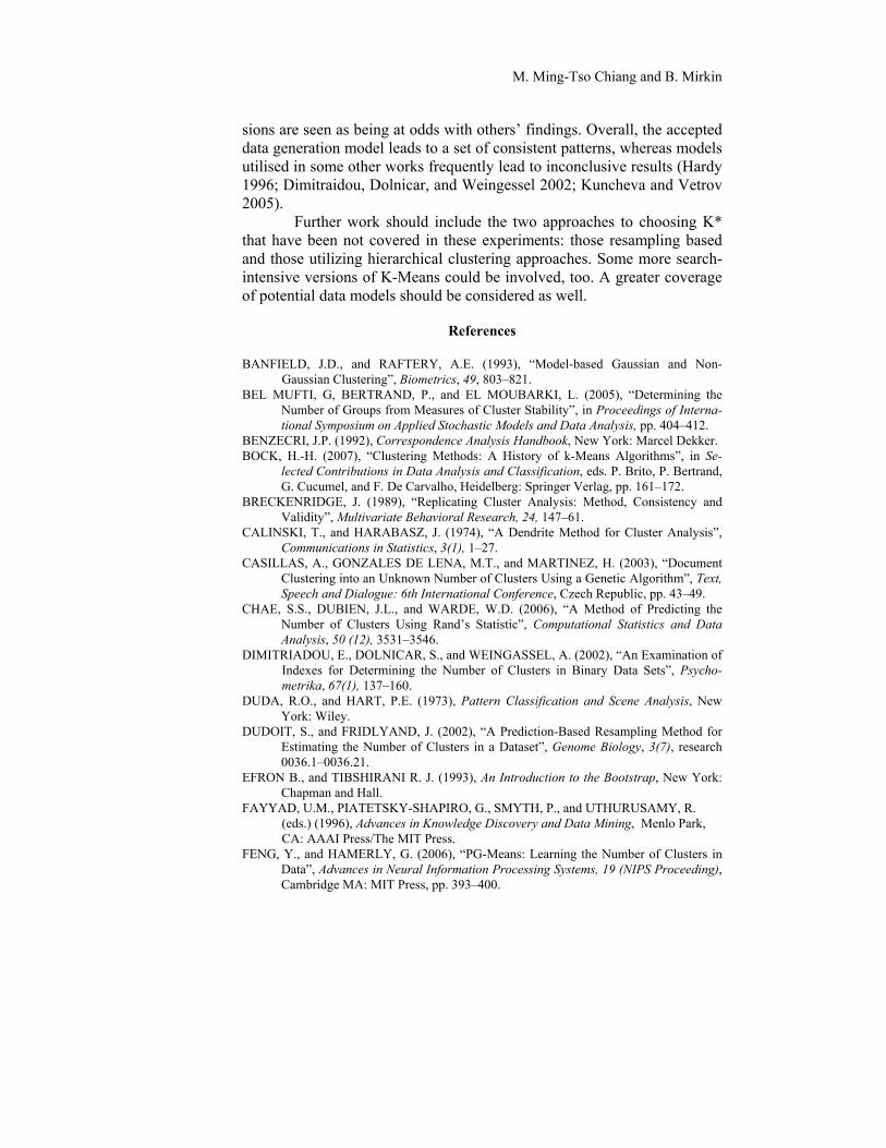
M. Ming-Tso Chiang and B. Mirkin
sions are seen as being at odds with others’ findings. Overall, the accepted data generation model leads to a set of consistent patterns, whereas models utilised in some other works frequently lead to inconclusive results (Hardy 1996; Dimitraidou, Dolnicar, and Weingessel 2002; Kuncheva and Vetrov 2005).
Further work should include the two approaches to choosing K* that have been not covered in these experiments: those resampling based and those utilizing hierarchical clustering approaches. Some more search-intensive versions of K-Means could be involved, too. A greater coverage of potential data models should be considered as well.
References
BANFIELD, J.D., and RAFTERY, A.E. (1993), “Model-based Gaussian and Non-Gaussian Clustering”, Biometrics, 49, 803–821.
BEL MUFTI, G, BERTRAND, P., and EL MOUBARKI, L. (2005), “Determining the Number of Groups from Measures of Cluster Stability”, in Proceedings of Interna-tional Symposium on Applied Stochastic Models and Data Analysis, pp. 404–412.
BENZECRI, J.P. (1992), Correspondence Analysis Handbook, New York: Marcel Dekker. BOCK, H.-H. (2007), “Clustering Methods: A History of k-Means Algorithms”, in Se-
lected Contributions in Data Analysis and Classification, eds. P. Brito, P. Bertrand, G. Cucumel, and F. De Carvalho, Heidelberg: Springer Verlag, pp. 161–172.
BRECKENRIDGE, J. (1989), “Replicating Cluster Analysis: Method, Consistency and Validity”, Multivariate Behavioral Research, 24, 147–61.
CALINSKI, T., and HARABASZ, J. (1974), “A Dendrite Method for Cluster Analysis”, Communications in Statistics, 3(1), 1–27.
CASILLAS, A., GONZALES DE LENA, M.T., and MARTINEZ, H. (2003), “Document Clustering into an Unknown Number of Clusters Using a Genetic Algorithm”, Text, Speech and Dialogue: 6th International Conference, Czech Republic, pp. 43–49.
CHAE, S.S., DUBIEN, J.L., and WARDE, W.D. (2006), “A Method of Predicting the Number of Clusters Using Rand’s Statistic”, Computational Statistics and Data Analysis, 50 (12), 3531–3546.
DIMITRIADOU, E., DOLNICAR, S., and WEINGASSEL, A. (2002), “An Examination of Indexes for Determining the Number of Clusters in Binary Data Sets”, Psycho-metrika, 67(1), 137–160.
DUDA, R.O., and HART, P.E. (1973), Pattern Classification and Scene Analysis, New York: Wiley.
DUDOIT, S., and FRIDLYAND, J. (2002), “A Prediction-Based Resampling Method for Estimating the Number of Clusters in a Dataset”, Genome Biology, 3(7), research 0036.1–0036.21.
EFRON B., and TIBSHIRANI R. J. (1993), An Introduction to the Bootstrap, New York: Chapman and Hall.
FAYYAD, U.M., PIATETSKY-SHAPIRO, G., SMYTH, P., and UTHURUSAMY, R. (eds.) (1996), Advances in Knowledge Discovery and Data Mining, Menlo Park, CA: AAAI Press/The MIT Press.
FENG, Y., and HAMERLY, G. (2006), “PG-Means: Learning the Number of Clusters in Data”, Advances in Neural Information Processing Systems, 19 (NIPS Proceeding), Cambridge MA: MIT Press, pp. 393–400.
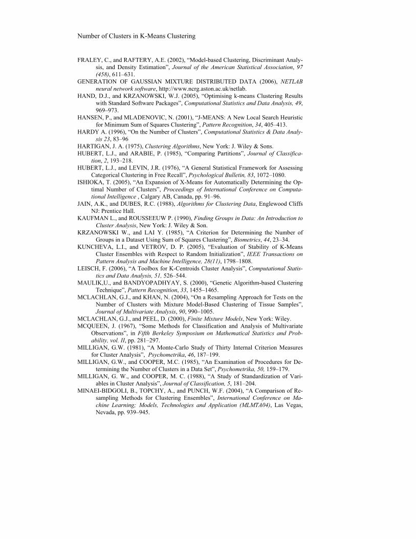
Number of Clusters in K-Means Clustering
FRALEY, C., and RAFTERY, A.E. (2002), “Model-based Clustering, Discriminant Analy-sis, and Density Estimation”, Journal of the American Statistical Association, 97 (458), 611–631.
GENERATION OF GAUSSIAN MIXTURE DISTRIBUTED DATA (2006), NETLAB neural network software, http://www.ncrg.aston.ac.uk/netlab.
HAND, D.J., and KRZANOWSKI, W.J. (2005), “Optimising k-means Clustering Results with Standard Software Packages”, Computational Statistics and Data Analysis, 49, 969–973.
HANSEN, P., and MLADENOVIC, N. (2001), “J-MEANS: A New Local Search Heuristic for Minimum Sum of Squares Clustering”, Pattern Recognition, 34, 405–413.
HARDY A. (1996), “On the Number of Clusters”, Computational Statistics & Data Analy-sis 23, 83–96
HARTIGAN, J. A. (1975), Clustering Algorithms, New York: J. Wiley & Sons. HUBERT, L.J., and ARABIE, P. (1985), “Comparing Partitions”, Journal of Classifica-
tion, 2, 193–218. HUBERT, L.J., and LEVIN, J.R. (1976), “A General Statistical Framework for Assessing
Categorical Clustering in Free Recall”, Psychological Bulletin, 83, 1072–1080. ISHIOKA, T. (2005), “An Expansion of X-Means for Automatically Determining the Op-
timal Number of Clusters”, Proceedings of International Conference on Computa-tional Intelligence , Calgary AB, Canada, pp. 91–96.
JAIN, A.K., and DUBES, R.C. (1988), Algorithms for Clustering Data, Englewood Cliffs NJ: Prentice Hall.
KAUFMAN L., and ROUSSEEUW P. (1990), Finding Groups in Data: An Introduction to Cluster Analysis, New York: J. Wiley & Son.
KRZANOWSKI W., and LAI Y. (1985), “A Criterion for Determining the Number of Groups in a Dataset Using Sum of Squares Clustering”, Biometrics, 44, 23–34.
KUNCHEVA, L.I., and VETROV, D. P. (2005), “Evaluation of Stability of K-Means Cluster Ensembles with Respect to Random Initialization”, IEEE Transactions on Pattern Analysis and Machine Intelligence, 28(11), 1798–1808.
LEISCH, F. (2006), “A Toolbox for K-Centroids Cluster Analysis”, Computational Statis-tics and Data Analysis, 51, 526–544.
MAULIK,U., and BANDYOPADHYAY, S. (2000), “Genetic Algorithm-based Clustering Technique”, Pattern Recognition, 33, 1455–1465.
MCLACHLAN, G.J., and KHAN, N. (2004), “On a Resampling Approach for Tests on the Number of Clusters with Mixture Model-Based Clustering of Tissue Samples”, Journal of Multivariate Analysis, 90, 990–1005.
MCLACHLAN, G.J., and PEEL, D. (2000), Finite Mixture Models, New York: Wiley. MCQUEEN, J. (1967), “Some Methods for Classification and Analysis of Multivariate
Observations”, in Fifth Berkeley Symposium on Mathematical Statistics and Prob-ability, vol. II, pp. 281–297.
MILLIGAN, G.W. (1981), “A Monte-Carlo Study of Thirty Internal Criterion Measures for Cluster Analysis”, Psychometrika, 46, 187–199.
MILLIGAN, G.W., and COOPER, M.C. (1985), “An Examination of Procedures for De-termining the Number of Clusters in a Data Set”, Psychometrika, 50, 159–179.
MILLIGAN, G. W., and COOPER, M. C. (1988), “A Study of Standardization of Vari-ables in Cluster Analysis”, Journal of Classification, 5, 181–204.
MINAEI-BIDGOLI, B., TOPCHY, A., and PUNCH, W.F. (2004), “A Comparison of Re-sampling Methods for Clustering Ensembles”, International Conference on Ma-chine Learning; Models, Technologies and Application (MLMTA04), Las Vegas, Nevada, pp. 939–945.
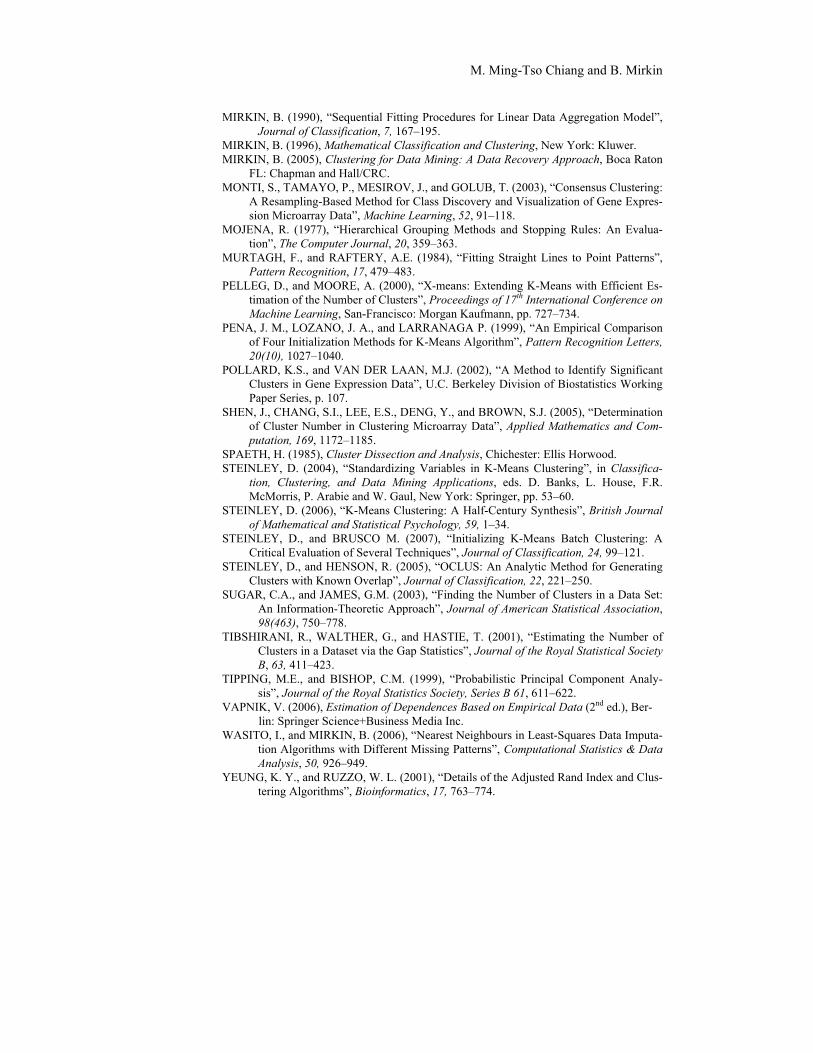
M. Ming-Tso Chiang and B. Mirkin
MIRKIN, B. (1990), “Sequential Fitting Procedures for Linear Data Aggregation Model”, Journal of Classification, 7, 167–195.
MIRKIN, B. (1996), Mathematical Classification and Clustering, New York: Kluwer. MIRKIN, B. (2005), Clustering for Data Mining: A Data Recovery Approach, Boca Raton
FL: Chapman and Hall/CRC. MONTI, S., TAMAYO, P., MESIROV, J., and GOLUB, T. (2003), “Consensus Clustering:
A Resampling-Based Method for Class Discovery and Visualization of Gene Expres-sion Microarray Data”, Machine Learning, 52, 91–118.
MOJENA, R. (1977), “Hierarchical Grouping Methods and Stopping Rules: An Evalua-tion”, The Computer Journal, 20, 359–363.
MURTAGH, F., and RAFTERY, A.E. (1984), “Fitting Straight Lines to Point Patterns”, Pattern Recognition, 17, 479–483.
PELLEG, D., and MOORE, A. (2000), “X-means: Extending K-Means with Efficient Es-timation of the Number of Clusters”, Proceedings of 17th International Conference on Machine Learning, San-Francisco: Morgan Kaufmann, pp. 727–734.
PENA, J. M., LOZANO, J. A., and LARRANAGA P. (1999), “An Empirical Comparison of Four Initialization Methods for K-Means Algorithm”, Pattern Recognition Letters, 20(10), 1027–1040.
POLLARD, K.S., and VAN DER LAAN, M.J. (2002), “A Method to Identify Significant Clusters in Gene Expression Data”, U.C. Berkeley Division of Biostatistics Working Paper Series, p. 107.
SHEN, J., CHANG, S.I., LEE, E.S., DENG, Y., and BROWN, S.J. (2005), “Determination of Cluster Number in Clustering Microarray Data”, Applied Mathematics and Com-putation, 169, 1172–1185.
SPAETH, H. (1985), Cluster Dissection and Analysis, Chichester: Ellis Horwood. STEINLEY, D. (2004), “Standardizing Variables in K-Means Clustering”, in Classifica-
tion, Clustering, and Data Mining Applications, eds. D. Banks, L. House, F.R. McMorris, P. Arabie and W. Gaul, New York: Springer, pp. 53–60.
STEINLEY, D. (2006), “K-Means Clustering: A Half-Century Synthesis”, British Journal of Mathematical and Statistical Psychology, 59, 1–34.
STEINLEY, D., and BRUSCO M. (2007), “Initializing K-Means Batch Clustering: A Critical Evaluation of Several Techniques”, Journal of Classification, 24, 99–121.
STEINLEY, D., and HENSON, R. (2005), “OCLUS: An Analytic Method for Generating Clusters with Known Overlap”, Journal of Classification, 22, 221–250.
SUGAR, C.A., and JAMES, G.M. (2003), “Finding the Number of Clusters in a Data Set: An Information-Theoretic Approach”, Journal of American Statistical Association, 98(463), 750–778.
TIBSHIRANI, R., WALTHER, G., and HASTIE, T. (2001), “Estimating the Number of Clusters in a Dataset via the Gap Statistics”, Journal of the Royal Statistical Society B, 63, 411–423.
TIPPING, M.E., and BISHOP, C.M. (1999), “Probabilistic Principal Component Analy-sis”, Journal of the Royal Statistics Society, Series B 61, 611–622.
VAPNIK, V. (2006), Estimation of Dependences Based on Empirical Data (2nd ed.), Ber-lin: Springer Science+Business Media Inc.
WASITO, I., and MIRKIN, B. (2006), “Nearest Neighbours in Least-Squares Data Imputa-tion Algorithms with Different Missing Patterns”, Computational Statistics & Data Analysis, 50, 926–949.
YEUNG, K. Y., and RUZZO, W. L. (2001), “Details of the Adjusted Rand Index and Clus-tering Algorithms”, Bioinformatics, 17, 763–774.