A pilot study was initiated to evaluate the feasibility ofusing legacy 3-D seismic time-lapse analysis as a reservoirmonitoring tool to assist planning future development ina shallow oil and gas field in the Gulf of Mexico. The reser-voir selected for initial evaluation was the shallowest of aseries of stacked oil and gas pays. This choice was basedon seismic data quality and the desire to eliminate any pos-sible effects of production in overlying reservoirs.

The target reservoir produces gas from a faulted anti-clinal trap at a depth of about 3000 ft, is normally pres-sured, and exhibits a strong water drive. The reservoir hasbeen produced by three wells, two of which are no longerproducing gas due to high water production.

Two 3-D seismic surveys have been acquired since ini-tial production—one in 1987 and the other in 1995. Duringthe interim between surveys, approximately 26.6 billionft3 of gas was produced. Maps based on the 3-D data showgood structural conformance of seismic amplitude withknown hydrocarbon/water contacts, and indicate poten-tial drilling locations in undrilled fault blocks updip fromthe depleted wells. The technique developed in this studyuses the two existing (legacy) 3-D data sets in conjunctionwith well logs and production data to provide spatial con-straints on estimates of produced and remaining reserves.

Fluid substitution study. The first phase of this studyinvolved modeling the expected acoustic response of thereservoir to simulate fluid saturation changes. Initial effortsusing a uniform or “pure saturation” Gassmann-basedfluid substitution model did not adequately predict theobserved seismic response. As a result, we used a “patchysaturation” model to better describe observable differencesin seismic data. This model predicted an acoustic imped-ance increase of approximately 10% in the swept zone(30% gas being replaced by water). Tuning analysis useda wedge model with an assumed central frequency of 30Hz in the seismic wavelet (0-60 Hz). The correspondingtuning thickness was determined by

(1)

where V is the velocity of the layer and fc is the central fre-quency of the seismic data assuming the central frequencyis dominant. However, two potential sources of error arepossible when applying this relation to legacy seismicdata. The variation of computed tuning thickness mayresult from variation in seismic velocity caused by pro-duction-related fluid substitution or from variation in fre-quencies between data sets.

We will use the model in Figure 1, a wedge with thick-ness varying from 0-150 ft and a gas cap, to illustrate thisambiguity. Water saturation in the gas cap was systemat-ically increased in successive modeling runs.Corresponding values of acoustic impedance and ampli-tude were calculated assuming a patchy saturation distri-bution. These data are listed in Table 1. The results of thesemodel runs are shown in Figure 2 in which seismic ampli-

278 THE LEADING EDGE MARCH 2001 MARCH 2001 THE LEADING EDGE 0000

Integration of time-lapse seismic andproduction data in a Gulf of Mexico gas field

XURI HUANG, ROBERT WILL, MASHIUR KHAN, and LARRY STANLEY, WesternGeco, Houston, Texas, U.S.

Table 1. Acoustic impedance change caused by gassaturation changeSg (%)

8880706050403020

Impedance11330.011740.012213.012768.013138.013655.014095.014444.0

Change (%)0.03.67.812.715.920.524.427.5

Figure 1. Wedge model with a gas cap (depth in feet).

Figure 2. Relationship between reservoir thickness, gassaturation and amplitude change derived from a“patchy saturation” model for a frequency of 60 Hz.

tude change is related to wedge thickness and gas satu-ration change for a frequency of 60 Hz. The effect of vary-ing the frequency on amplitude difference was investigatedby fixing the saturation and running the analysis at vary-ing frequencies. Figure 3 shows the results of model runsin which gas saturation change was set at 28% and fre-quency was varied from 60 to 120 Hz (high end frequency).Figure 4 illustrates the relation between saturation change,frequency, and amplitude change for a fixed thickness of50 ft. We can see that, if the data sets have similar frequencycontent, for a given thickness of 70 ft and change of gassaturation of 40% the amplitude change will be around80%. This closely approximates our observations from the3-D data over this field. These results clearly illustrate thepotential effects caused by variations in seismic frequency

and gas saturation on seismic amplitude in legacy data,and the need for such effects to be properly corrected dur-ing time-lapse analyses.

Time-lapse analysis. In addition to the eight-year differ-ence in age, the two 3-D data sets were acquired andprocessed by different contractors. As a result, some notablevariations in acquisition and processing parameters are pre-sent—source-receiver offset ranges, spatial sampling den-sity, and 3-D migration algorithms. Poststack treatment ofthe data sets was minimal, incorporating only steps nec-essary for spatial repositioning prior to differencing.

Sample intervals of 50 m in-line and 60 m cross-line wereselected for the analysis. Preliminary differences taken afterrepositioning show fair repeatability, with the expectedamount of degradation in areas of steeply dipping events.By analyzing the spectra of both 3-D data sets, we observethat the frequency contents for both surveys are quite simi-lar, with the second being slightly richer in high frequencies.

Cross-equalization of the two data sets was performedthrough a two-stage process—global equalization followedby local spatial-temporal shifting. Prior to global equaliza-tion the data sets were band-limited to a common frequencybandwidth, scaled, and differenced (Figure 5). At this stage,significant differences are seen outside the reservoir inter-val. Next, a global equalization operator was designed froma region of good data quality and repeatability. The locationwas a nonproducing region below the field’s original hydro-carbon-water contact, thereby eliminating potential conta-mination from production-related changes. Figure 6 showsthe difference for the same in-line after application of this

280 THE LEADING EDGE MARCH 2001 MARCH 2001 THE LEADING EDGE 0000

Figure 3. Relationship between seismic amplitudechange, frequency, and thickness for a 28% gas satura-tion change.

Figure 4. Relationship between seismic amplitudechange, frequency, and gas saturation at a thickness of50 ft.

Figure 5. Raw difference after applying global equal-ization with a single scaler.

global cross-equalization filter. The amplitude differencesbetween reservoir and nonreservoir zones are significantlyimproved over Figure 5.

After global equalization, the remaining differencesbetween two data sets in the nonreservoir intervals shouldbe limited to small time and spatial shifts that are the com-bined result of horizontal positioning and temporal datum-ing errors. These errors may arise from a variety ofmechanisms such as field positioning errors, tidal variations,seismic wavelet phase differences, and seismic processingoperator phase differences. Although many of these errorsare systematic in nature, there is rarely sufficient data avail-able for resolution and deterministic correction of indepen-dent error sources. In this study, final spatial equalization ofthe data sets was performed using a time and spatially vari-ant correlation operator. The equalization algorithm oper-ates on a trace-by-trace basis and performs crosscorrelationover a user-defined window between the target (from themonitor survey) and all other traces (from the base survey)lying within a user-defined search radius. The target traceis time shifted according to the maximum correlation. Searchradius and correlation length are optimized to honor the spa-tial and temporal limits of the error processes as well as thespatial/temporal limits of resolution in the data. Figure 7,the difference after time- and space-variant cross-equaliza-tion, shows further significant improvement in repeatabil-ity. In addition to the spatially equalized seismic volumes,this process yields diagnostic volumes of correlation coeffi-cient and lag. These diagnostic volumes are critical for eval-uation of the suitability of processing parameters and theintegrity of the output volumes. Attributes such as ampli-tude envelope and rms difference extracted from the top of

reservoir horizons may be used to examine the production-related seismic variations. Figure 8 shows the difference inthe amplitude envelope along the reservoir horizon afterapplication of global equalization. Figure 9 shows the dif-ference along the same horizon after application of local cor-relation operators to the globally equalized volume. Thedifference outside the reservoir has been further minimizedby the second equalization step.

Production data analysis. Reserves estimates can usually bedetermined from production history data by such techniquesas decline curve analysis or material mass balancing, or vol-umetric approaches. For gas reservoirs, it is quite commonto conduct P/Z analysis for estimating reserves. However,this field was produced by a mixed mechanism of water driveand pressure depletion. Therefore, the equation for theclosed gas reservoir may not be applicable for this case andthe P/Z relation needs to be modified to account for thiseffect. Assuming that the gas pore volume at the time of thefirst seismic survey (So) is G, then total production from thetime of first survey to that of the second (St) is Gp. The resid-ual gas pore volume at St is Gr. Converting Gp to reservoirconditions Gpr at the time of the second survey and assum-ing an isothermal system yields

(2)

which can be rearranged as

(3)

282 THE LEADING EDGE MARCH 2001 MARCH 2001 THE LEADING EDGE 0000

Figure 7. Difference after time- and space-variantcross-equalization.

Figure 6. Difference after global phase and amplitudematch.

Here, Po, Zo, Pt, Zt are the reservoir average pressure andgas compressibility factors for times So and St, respectively.Gpr is the volume of the cumulative production underreservoir conditions at St. This relation, which could be con-sidered as the material balance relation for the gas com-ponent, has two unknowns, Gr and G. If we consider waterinflux along with production, then the relation will includethe unknown We (water influx) rather than Gr. Using onlyproduction data, it would be difficult to achieve a uniquesolution for this simple equation. However, by combiningtime-lapse seismic data and production data, it is possibleto uniquely determine G and Gr. In certain cases, thereserves at the time of the first seismic survey may be esti-mated using the decline curve analysis.

Reconciling. Seismic differences were reconciled with pro-duction data by matching volumetric estimates determinedwith the two data types. Assuming that the seismic dif-ference represents the gas saturation decrease due to waterreplacement between surveys, the volume of the differencewill be proportional to the accumulated production.However, ambiguity exists with respect to the relationshipbetween seismic amplitude and saturation change. It istherefore necessary to find a seismic amplitude thresholdwhich best approximates the boundary of the swept area.

For any given seismic difference amplitude threshold,a change in gas volume may be computed by assumingan average gas saturation change within the area definedby that threshold. The optimal amplitude threshold isdetermined through an iterative process of comparing this

seismic (threshold limited) gas volume change with theobserved Gpr. Assuming that the accumulated productionis Gp, the volume under reservoir conditions will be,

(4)

(5)

(6)

Bg is the gas formation factor; T and Pr are the reservoirtemperature and pressure, respectively. Gpr represents thetotal volume of change in the reservoir. Figure 10 showsthe seismic difference map after the amplitude thresholdhas been optimized through reconciliation with the pro-duced gas volume. The average porosity for this processis 30%. The thickness is input from a geologic map. If nomatch or an unreasonable match is achieved, the proce-dure will go back to the cross-equalization for parametertuning until a reasonable one is obtained. In this sense, thecross-equalization is constrained by the production data.

After the seismic difference map has been reconciledwith volumes of fluid produced, we use this informationto improve estimates of the remaining reserves. Whenproperly thresholded, the volumes derived from base andmonitor seismic surveys should correspond to G and Grin Equation 3. The iteration loop involves adjustments tothe threshold followed by recomputation of G and Gr untilEquation 3 is satisfied. Computation of Gr is complicated

284 THE LEADING EDGE MARCH 2001 MARCH 2001 THE LEADING EDGE 0000

Figure 9. Difference along the reservoir horizon afterlocal equalization.

Figure 8. Difference along the reservoir horizon afterglobal equalization.

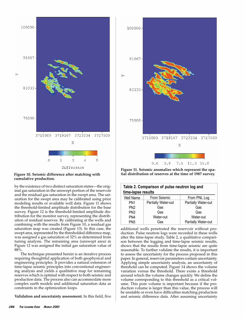
by the existence of two distinct saturation states—the orig-inal gas saturation in the unswept portion of the reservoirand the residual gas saturation in the swept area. The sat-uration for the swept area may be calibrated using priormodeling results or available well data. Figure 11 showsthe threshold-limited amplitude distribution for the basesurvey. Figure 12 is the threshold-limited amplitude dis-tribution for the monitor survey, representing the distrib-ution of residual reserves. By calibrating at the wells andcombining with the results from Figure 10, a residual gassaturation map was created (Figure 13). In this case, theswept area, represented by the thresholded difference map,was assigned a gas saturation of 32% as determined fromtuning analysis. The remaining area (unswept area) inFigure 12 was assigned the initial gas saturation value of88%.

The technique presented herein is an iterative processrequiring thoughtful application of both geophysical andengineering principles. It provides a natural extension oftime-lapse seismic principles into conventional engineer-ing analysis and yields a qualitative map for remainingreserves which is optimal with respect to both seismic andproduction data. The process also can accommodate morecomplex earth models and additional saturation data asconstraints in the optimization loops.

Validation and uncertainty assessment. In this field, five

additional wells penetrated the reservoir without pro-duction. Pulse neutron logs were recorded in these wellsafter the time-lapse study. Table 2, a qualitative compari-son between the logging and time-lapse seismic results,shows that the results from time-lapse seismic are quitereasonable. To further validate the results, it is importantto assess the uncertainty for the process proposed in thispaper. In general, reservoir parameters contain uncertainty.Applying simple uncertainty analysis, an uncertainty ofthreshold can be computed. Figure 14 shows the volumevariation versus the threshold. There exists a thresholdaround which the volume changes quickly. We define thevolume corresponding to this threshold as a critical vol-ume. This pore volume is important because if the pro-duction volume is larger than this value, the process willbe unstable or even have difficulties matching productionand seismic difference data. After assuming uncertainty

286 THE LEADING EDGE MARCH 2001 MARCH 2001 THE LEADING EDGE 0000

Figure 10. Seismic difference after matching withcumulative production.

Figure 11. Seismic anomalies which represent the spa-tial distribution of reserves at the time of 1987 survey.

Table 2. Comparison of pulse neutron log and time-lapse resultsWell Name

PN1PN2PN3PN4PN5

From SeismicPartially Water-out

GasGas

Water-outGas

From PNL LogPartially Water-out

GasGas

Water-outPartially Water-out

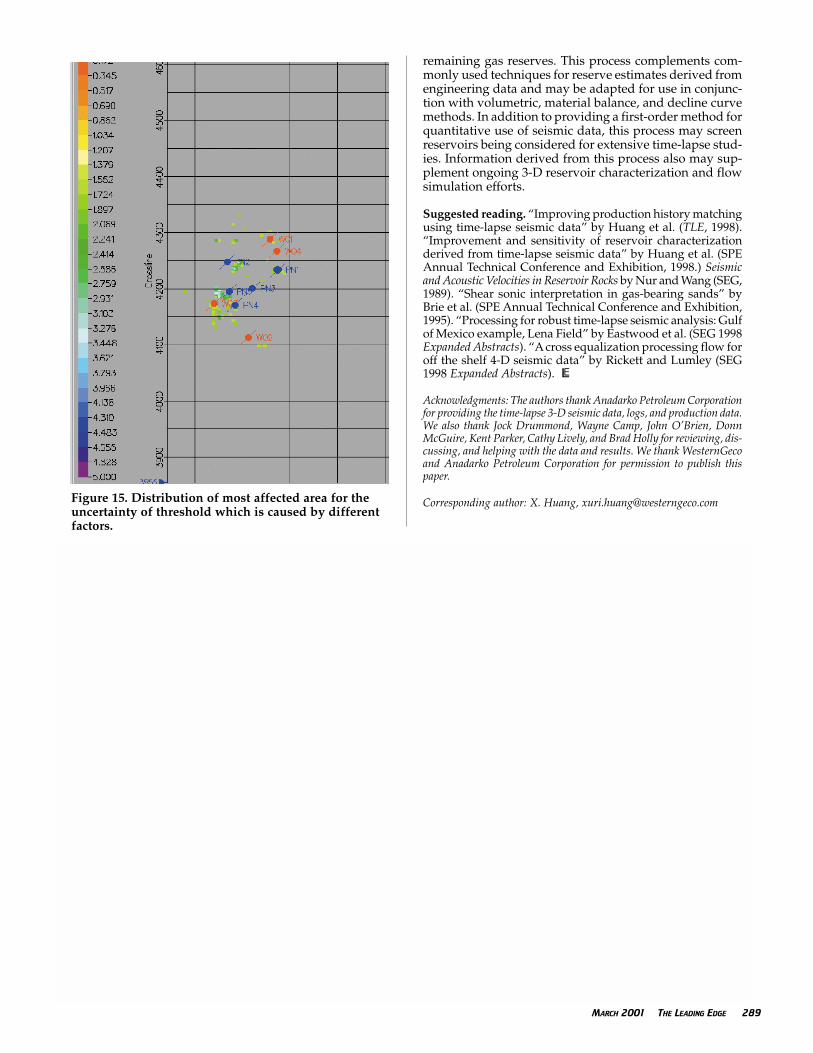
in the threshold of +10%, the spatial uncertainty wasmapped (Figure 15). We can see that well PN5 is in a mostuncertain area. This may be one reason that the time-lapse

seismic result at this location is not fully consistent withthe pulse neutron log. Another possible reason is the pro-ducing well close to PN5 continued low production afterthe second seismic survey while the others stopped pro-ducing. It may not be reasonable to compare the currentlog (1999) with seismic that reflects reservoir status fouryears ago.

Conclusions. Under certain geologic conditions, multiplelegacy 3-D seismic data sets may be used in conjunctionwith production data to provide valuable and timely con-straints in estimating the volume and distribution of

288 THE LEADING EDGE MARCH 2001 MARCH 2001 THE LEADING EDGE 0000

Figure 14. The volume variation with the change ofthreshold.

Figure 12. Seismic anomalies that represent spatialdistribution of remaining reserves at time of secondsurvey.

Figure 13. Residual gas saturation map after materialbalance matching and calibration.

remaining gas reserves. This process complements com-monly used techniques for reserve estimates derived fromengineering data and may be adapted for use in conjunc-tion with volumetric, material balance, and decline curvemethods. In addition to providing a first-order method forquantitative use of seismic data, this process may screenreservoirs being considered for extensive time-lapse stud-ies. Information derived from this process also may sup-plement ongoing 3-D reservoir characterization and flowsimulation efforts.

Suggested reading. “Improving production history matchingusing time-lapse seismic data” by Huang et al. (TLE, 1998).“Improvement and sensitivity of reservoir characterizationderived from time-lapse seismic data” by Huang et al. (SPEAnnual Technical Conference and Exhibition, 1998.) Seismicand Acoustic Velocities in Reservoir Rocks by Nur and Wang (SEG,1989). “Shear sonic interpretation in gas-bearing sands” byBrie et al. (SPE Annual Technical Conference and Exhibition,1995). “Processing for robust time-lapse seismic analysis: Gulfof Mexico example, Lena Field” by Eastwood et al. (SEG 1998Expanded Abstracts). “A cross equalization processing flow foroff the shelf 4-D seismic data” by Rickett and Lumley (SEG1998 Expanded Abstracts). LE

Acknowledgments: The authors thank Anadarko Petroleum Corporationfor providing the time-lapse 3-D seismic data, logs, and production data.We also thank Jock Drummond, Wayne Camp, John O’Brien, DonnMcGuire, Kent Parker, Cathy Lively, and Brad Holly for reviewing, dis-cussing, and helping with the data and results. We thank WesternGecoand Anadarko Petroleum Corporation for permission to publish thispaper.

Corresponding author: X. Huang, xuri.huang@westerngeco.com

0000 THE LEADING EDGE MARCH 2001 MARCH 2001 THE LEADING EDGE 289

Figure 15. Distribution of most affected area for theuncertainty of threshold which is caused by differentfactors.