Integration of artificial neural network and geographic

Integration of artificial neural network and geographic information system applications in simulating groundwater qualityVahid Gholami1, Marhemat Sebghati2, Zabihollah Yousefi3*

1Assistant Professor, Department of Range and Watershed Management, Faculty of Natural Resources, University of Guilan, Rasht, Iran2MS of Watershed Management, Department of Range and Watershed Management, Faculty of Natural Resources, Urmia University, Urmia, Iran3Professor, Department of Environmental Health Engineering, Faculty of Health, Mazandaran University of Medical Sciences, Sari, Iran

AbstractBackground: Although experiments on water quality are time consuming and expensive, models are often employed as supplement to simulate water quality. Artificial neural network (ANN) is an efficient tool in hydrologic studies, yet it cannot predetermine its results in the forms of maps and geo-referenced data. Methods: In this study, ANN was applied to simulate groundwater quality and geographic information system (GIS) was used as pre-processing and post-processing tool in simulating water quality in the Mazandaran Plain (Caspian southern coasts, Iran). Groundwater quality was simulated using multi-layer perceptron (MLP) network. The determination of groundwater quality index (GWQI) and the estimation of effective factors in groundwater quality were also undertaken. After modeling in ANN, the model validation was carried out. Also, the study area was divided with the pixels 1×1 km (raster format) in GIS medium. Then, the model input layers were combined and a raster layer which comprised the model inputs values and geographic coordinate was generated. Using geographic coordinate, the values of pixels (model inputs) were inputted into ANN (Neuro Solutions software). Groundwater quality was simulated using the validated optimum network in the sites without water quality experiments. In the next step, the results of ANN simulation were entered into GIS medium and groundwater quality map was generated based on the simulated results of ANN. Results: The results revealed that the integration of capabilities of ANN and GIS have high accuracy and efficiency in the simulation of groundwater quality. Conclusion: This method can be employed in an extensive area to simulate hydrologic parameters. Keywords: Water quality, GWQI, MLP, Mazandaran Plain.Citation: Gholami V, Sebghati M, Yousefi Z. Integration of artificial neural network and geographic information system applications in simulating groundwater quality. Environmental Health Engineering and Management Journal 2016; 3(4): 173–182. doi: 10.15171/EHEM.2016.17

*Correspondence to:Zabihollah Yousefi Email: [email protected]

Article History:Received: 22 June 2016Accepted: 26 July 2016ePublished: 31 August 2016

Environmental Health Engineering and Management Journal 2016, 3(4), 173–182

IntroductionGroundwater is one of the most important water resources on earth, and its water quality studies are very vital for the protection and planning of water resources particularly in arid and semi-arid regions such as Iran. Groundwater presently accounts for more than 90% of Iran’s total drink-ing water consumption. This water resource is less vulner-able to bacterial pollution and evaporation than surface water and therefore, groundwater is more important than surface water. One of the major limiting factors in water exploitation is unsuitable water quality. Human activities such as agricultures, manufacturing and urban develop-ment affect the quality of groundwater. Unfortunately, the groundwater quality is now being endangered due to in-appropriate exploitation and increased human activity in recent decades. Thus, it is necessary to study water quality in order to manage water resources properly. Since experi-

ments on water quality are time consuming and expen-sive, models are often employed as supplement to simulate water quality. Artificial neural network (ANN) was ap-plied for simulation in the field of water resources model-ing in the early 1990s. Its usage has increased significantly over the last decade, resulting in a number of studies on its applications (1-12). ANNs had provided an appeal-ing solution to simulate water resources system (13,14). The multi-layer perceptron (MLP) feed-forward network types have been widely applied to simulate hydrological parameters (15). Numerous studies have been conducted on the application of neural networks for groundwater forecasting (16-29). It is necessary to introduce an index in water quality stud-ies in order to evaluate the quality of water. In the past decades, various water quality indices have been used in previous studies for special purposes (30). Since the

Environmental Health Engineering and Management Journal

HE

MJ

© 2016 The Author(s). Published by Kerman University of Medical Sciences. This is an open-access article distributed under the terms of the Creative Commons Attribution License (http://creativecommons.org/licenses/by/4.0), which permits unrestricted use, distribution, and reproduction in any medium, provided the original work is properly cited.

10.15171/EHEM.2016.17doi

Original ArticleOpen AccessPublish Free

http://ehemj.com

http://dx.doi.org/10.15171/EHEM.2016.17

http://crossmark.crossref.org/dialog/?doi=10.15171/EHEM.2016.17&domain=pdf&date_stamp=2016-08-31

http://ehemj.com

Gholami et al


needed water quality parameters are available, we applied the ground water quality index (GWQI) which was first introduced by Ribeiro et al (31), to evaluate the ground water quality. So far, many studies have been conducted to measure surface and GWQI. The general water qual-ity index (WQI) was developed by Brown et al (32), and later improved by the Scottish Development Department (33), following the suggestion in Horton (34), that various water quality data could be aggregated into a single over-all index (35-41). Gholami et al (42), presented a model for estimating groundwater salinity on the Caspian Sea southern coasts employing the statistical and geographic information system (GIS) techniques. They estimated wa-ter salinity (electrical conductivity or EC) local changes with an acceptable accuracy. Lateef (43) investigated the groundwater quality of Tikrit and Samarra in Iraq using the WQI. They categorized the groundwater quality for 10 wells in some cities using WQI and discovered that the groundwater quality was unsatisfactory in the south of Sa-marra city. He attributed this water quality deterioration to the region’s from north to south groundwater drainage system. Singh et al (44) applied a GIS based multi-criteria analysis by assigning weights to different water quality pa-rameters. They grouped the water quality into six classes ranging from very good to unfit for drinking. They dis-covered that the water quality varied from moderate to good in most part of the study area except in some areas where the groundwater quality was classified as ‘poor to unfit.’ An evaluation of change in land usage and land cov-er from year 1989 to 2006 using Landsat and LISS III satel-lite data, indicated that the groundwater quality was ‘poor to unfit’ as a result of rapid urbanization and industrial-ization (44). Krishna et al (45) applied GIS-ANN hybrid system in predicting arsenic concentration in groundwa-ter. Their results revealed that GIS-ANN integration has a high capability in water quality modeling. This study has been conducted to simulate groundwater quality and also, to provide a methodology for combining ANN and GIS capabilities in hydrologic parameters modeling on the Caspian southern coasts.

MethodsStudy areaThe study area is located at 50º 30′ to 53º 50′ E longitude and 35º 55′ to 36º 45′ N latitude in Mazandaran province (Figure 1) which is located in the southern Caspian coast in northern Iran. Area of study plain is approximately 10 000 km2. The southern coasts of the Caspian Sea main-ly include plains made of quaternary sediments. However, there are diverse geologic formations and elevation and slope changes in central regions of Alborz mountains.

Determination of groundwater quality indexIn this study, eight water quality parameters such as: cation and anion (K+, Na+, Ca2+, Cl-, Mg2+, SO4

2- ), pH and total dissolved salt (TDS) were selected. These parameters were used for estimating the WQI. We were faced with a limita-tion in defining the type of WQI because of lack of mea-

surements of microbial pollution in the region. At first, out of about 200 drinking water wells in the study area, 85 wells were selected based on their available water quality secondary data. In general, these 85 wells had adequate sampled data with water quality secondary data from 2008 to 2013 (46). As earlier stated, estimating GWQI for 85 wells were made using water quality secondary data (i.e. 6-year data with 4 samples per year). The location of these drinking water wells in the study area is presented in Fig-ure 1. Prior to studying the GWQI, it is essential to choose a standard criterion in order to determine maximum val-ues of the parameters. Iranian national standards of these eight water quality parameters for potable water are pre-sented in Table 1.Eq. (1) was applied to estimate the GWQI based on the standard values given in Table 1:

8

1. i

ii i

CGWQI wCs=

=∑ (1)

where GWQI denotes the groundwater quality index; wi is the relative weight of the parameter; Ci is the concentration of the parameter and Csi is the national standard concen-tration of the parameter for potable water. Each parameter has a different weight in terms of its contribution to water quality. The corresponding weight values of the parame-ters are then aggregated using some types of sum or mean (e.g., arithmetic, harmonic, geometric), frequently includ-ing individual weighing factors (34,41,47,48). The relative importance/contribution or the weights of parameters in

Figure 1. Study area (a) and location of drinking water wells (b) in the Mazandaran plain.

Table 1. Potable water quality standards of Iran (mgl-1) K+ Na+ Ca2+ Mg2+ SO4

2- Cl- pH TDS12 200 200 150 400 600 6.5-8.5 2000

Source: Saeedi et al (49).

Environmental Health Engineering and Management Journal 2016, 3(4), 173–182 175

Gholami et al

the final GWQI are defined on the basis of the extent of their participation in the water quality determination in order to estimate the final index by aggregating all the normalized parameters. The weight of the participation of each parameter in the final GWQI is given in Table 2.GWQI values are categorized into three classes; high (GWQI > 0.15), low (GWQI < 0.04), and suitable (0.04 < GWQI < 0.15) (49). For data collection and processing, we applied GIS. Different digital/base maps were provid-ed in GIS environment including digital elevation model (DEM), transmissivity of aquifer formations, water table depth (50), residential and industrial areas using topo-graphic maps of the region and GWQI values using the water quality secondary data (46).

Groundwater quality simulation using ANNAn ANN includes three layers, i.e., input layer, hidden layer and output layer. A network can have more than one hidden layer. In this study, MLP was applied to simulate groundwater quality. A typical MLP structure is illustrated in Figure 2. MLP is generated by adding one or more hid-den layers to one-layer perceptron and this topology can solve complex problems (51).Determination of the network optimum structure and number of neurons are important in network planning. MLP is the most extensively applied neural network ar-chitecture in literature for classification or regression problems (52-55). Three-layer (input, hidden and output) feed-forward neural network with LM back-propagation learning were employed for simulating groundwater qual-ity or GWQI. The first and simplest type of ANN devised was the feed-forward neural network. In the feed-forward network, the information moves in only one direction, forward, from the input nodes, through the hidden nodes

and to the output nodes. In the first stage of simulation, all data were normalized and divided into three classes: training data (65% of all data), test data (23% of all data) and cross validation data (12% of all data).The hyperbolic tangent and sigmoid transfer functions were used. Based on the study results (through trial-and-error method), the best transfer function was the hyperbolic tangent transfer function. The objective of network training is to find the network that can simulate the relationship between inputs and outputs model. Since there were no definite rules in planning neural network structure, we evaluated different structures of the network. In the study area, 85 drinking water wells were selected based on their available water quality secondary data. In general, these 85 wells had ad-equate sampled data with water quality secondary data. The GWQI parameter was used as an output variable and groundwater quality factors were used as inputs variables. The input factors are depth of the water table, distance from contaminant centers, site elevation or site location, population, households and aquifer formations (trans-missivity). The inputs values were estimated using DEM, transmissivity of aquifer formations and water table depth maps (50) then residential and industrial areas were done using topographic maps and satellite images of the region. Also, GWQI values were estimated using the water quality secondary data (46). The estimated input and output data were imported to ANN (Neuro Solutions software) me-dium. The most commonly applied method use in deter-mining the optimum structure, learning rate and momen-tum parameter is the trial-and-error approach (15). We changed the numbers of hidden neurons from 1 to 10. We found that using trial-and-error method in a MLP net-work with tangent hyperbolic transfer function, LM train-ing technique was the best network structure in ground-water quality simulation. Network training is one of the main stages in modeling using ANN. Weight coefficients in intermediate and output layers will be determined in the training stage (51,56,57). For the development of ANN model, we should determine both the significant and in-dependent inputs (58,59). Determination of ANN model structure generally involves defining the number of layers, the number of nodes in each layer and how they are con-nected (10). Here, an index known as the GWQI was used to evaluate the water quality. In the study area, 85 drinking water wells were selected and for each drinking water well, the GWQI value was then estimated. Appropriate input parameters were selected by trial-and-error method and sensitivity analysis. Eight input patterns were investigated and their efficiencies were evaluated and compared (Eq. 2-9):GWQI = ƒ(T, GwTable) (2)GWQI = ƒ(T, GwTable, Lc) (3)GWQI = ƒ(T, GwTable, Lc, E) (4)GWQI = ƒ(T, GwTable, Lc, E, P) (5)GWQI = ƒ(T, GwTable, Lc, E, P, H) (6)GWQI = ƒ(GwTable, Lc, E, P, H) (7)GWQI = ƒ(T, Lc, E, P, H) (8)GWQI = ƒ(T, GwTable, E, P, H) (9)

Table 2. Weight of participation of each parameter in the final GWQI

Parameter Parameter’s weightK+ 0.04Na+ 0.06Mg2+ 0.15Ca2+ 0.2SO4

2- 0.1Cl- 0.1pH 0.2TDS 0.15

Source: Saeedi et al (49).

Figure 2. A typical multi-layer feed forward neural network archi-tecture.

Gholami et al


where GWQI is the groundwater quality index, T is the transmissivity of aquifer formations (m2/day), GwTable is the groundwater table depth (m) and Lc is the distance of a well from contaminant and residential centers (m). P and H are the population and the number of household within the area of 1 km2 and E is the site elevation.A sensitivity analysis of model inputs was done in order to determine key parameters to groundwater quality. Sen-sitivity analysis is usually performed to study the effect of inputs on the outputs and to determine if any insignificant inputs can be ignored. Results revealed that the significant factors on groundwater quality and the best inputs in the simulation of groundwater quality were transmissivity of aquifer formations, groundwater depth, and distance from residential and industrial areas. An optimum network can be defined by three main components: transfer function, network architecture and learning rule (60). The determi-nation of the network size is usually carried out by trial and error experimentation. The procedure begins with one neuron in one hidden layer and progressing (with in-creasing size) until the performance of the test is found suitable (61). The ANN efficiency was evaluated using the mean squared error (MSE) and the coefficient of deter-mination (R2). The MSE and R2 are defined as (Eq. 10 & 11):

( )Qi QiMSEn

∧

∑ −=

(10)

~

2 1~

2 21

( ).( )

( ) .( )

ni ii

ni ii

Q Qi Qi QR

Q Qi Qi Q

∧

=

∧

=

− −

= − −

∑∑

(11)

where Qi is the observed value, Qi∧

is the simulated value and Qi is the mean of the observed data and

~

iQ is the mean of the simulated data and n is the number of data.The ANN efficiency (network validation) is evaluated using the MSE and the coefficient of determination (R2). Then, the optimized network was validated throughout the comparison between the actual values and the esti-mated values (test stage).

Integration of ANN and GIS in simulating groundwater qualityANN is an efficient tool in hydrologic studies. In this study, an integration of ANN and GIS has been employed to simulate groundwater quality. ANN and GIS have been used for simulation and as a pre-processing and post-processing system of the applied data respectively. Thus, GIS was applied as an efficient tool to provide base maps and to estimate model quantitative parameters. Different digital/base maps were provided in GIS environment in-cluding DEM, transmissivity of aquifer formations, water table depth (50), the number of household and popula-tions, residential and industrial areas using topographic maps of the region and GWQI values using water qual-ity secondary data (46). Eighty-five drinking water wells

were selected to simulate GWQI. Then, the estimated data of these parameters were inputted into the ANN me-dium (Neuro Solutions software) for modeling. Initially, the data was separated into three parts, namely, training data, cross validation data and testing data. The model was optimized on network structure (transfer function, inputs and the number of neuron) by using trial-and-er-ror method. Then, optimized model was evaluated using testing data. After validation model, we applied the vali-dated optimum model for simulating the GWQI in sites without water quality experiments. In this step, GIS had a pre-processing role in modeling process. The objective of the present study was using ANN to simulate groundwa-ter quality in a manner of geo-referenced graphic for sites without water quality data. The results revealed that the optimized network structure needs to have three inputs such as: transmissivity of aquifer formation, water table depth and the distance from contaminant centers. Ras-ter layers of the three input factors were provided in GIS pre-processing stage and were combined using overlay analysis with a pixel size 1×1 km. So, the surface of study plain was separated to more than 10 000 geo-referenced pixels (1×1 km). These pixels had values of model inputs or groundwater quality factors (transmissivity of aquifer formation, water table depth and the distance from con-taminant centers). We automatically inserted the site coordinate for every pixel in the GIS medium. Pixels data (networks inputs and coordinate) were exported from GIS and then im-ported to Neuro Solutions software. In ANN medium, GWQI was simulated using the validated optimum net-work for all of the 10 000 pixels (all of the study plain). In the next step, simulated GWQI were imported from ANN to GIS medium with geographic location data (X, Y). GIS had a post-processing role in this phase of study. We generated groundwater quality map using GWQI values (throughout geographic coordinate as an assisting agent for distinguishing geographic coordinate) and GIS capa-bilities study plain. Actual GWQI values of 85 drinking water wells were overlain on the generated raster layer of GWQI in GIS and result accuracy was evaluated via the comparison between the simulated GWQI and the actual GWQI in GIS. Evaluation results showed that the results were accurate and acceptable. Finally, groundwater raster layer was presented after been classified as groundwater quality map. Study stages are shown in Figure 3. In this study, groundwater quality simulation was performed us-ing ANN and GIS capabilities in an extensive area with high accuracy and the results were presented in a manner of geo-referenced graphic (map).

ResultsGWQI indices were estimated for the studied drinking water wells based on the 6-year sampling data with four samples per year. We estimated significant factors on wa-ter quality including aquifer formations transmissivity, water table depth, site elevation, distance from contami-nant centers and populations. A number of the estimated


Gholami et al

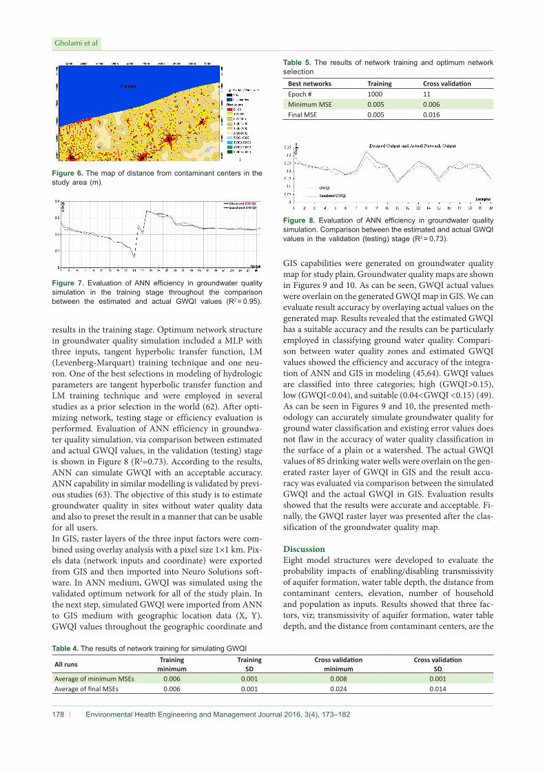
As can be seen in Figures 4, 5 and 6, digital maps of these three factors were generated in GIS. Figure 7 shows the results of ANN simulation in the training stage for ground water quality simulation and, as can be seen, R2 = 0.95. The results of network evaluation were presented in Tables 4 and 5. Tables 4 and 5 show error values in the training stage. Based on these results we found acceptable

12

Input data for GWQI simulation

Training and cross validation stages

Test stage

Optimum model determination

Simulation by ANN

Providing the raster layers of dependent variables in GIS

Combining raster layers

Estimating the parameters for Pixels

Exporting geo-referenced data

GIS: Preprocessing

Forecasting GWQI using validated network

Entering the estimated GWQI to GIS

Converting to raster layer and GWQI map

Results validation in GIS

Groundwater quality map

GIS: Post Processing

Data collection and sampling

Field studies Digital maps Water qualitative experiments (drinking water wells)

GWQI determination

GIS environment

Water quality variables estimation

Figure 3. The flow chart showing the methodology stages used in this study.

Figure 4. The map of average transmissivity of aquifer formation in the study area (m2/day).

Figure 5. The map of average water table depth in the study area (m).

Table 3. Factors affecting groundwater quality and GWQI in some drinking water wells

No GWQI Transmissivity(m2/day)

Water tableDepth (m)

Elevation(m)

Distance from contaminantcenters (m)

No. ofhousehold Population

1 0.2715 1500 12.90 50 6.4 52 4602 0.2401 750 3.00 -11 153.8 239 10773 0.2267 175 5.00 -13 99.4 32 1444 0.2165 750 4.00 -10 1121.2 21 985 0.2125 1500 5.00 11 0 22 936 0.2070 500 4.17 6 20 246 11057 0.1971 1000 5.00 11 0 22 938 0.1969 750 6.50 20 20 161 6669 0.1553 500 31.00 1062 830 30 95

10 0.1483 300 23.00 453 1100 13 6211 0.1252 300 25.00 69 709 53 28712 0.0568 100 38.00 1670 1023 53 34213 0.2578 500 4.70 6 44 109 49514 0.2042 750 3.50 -8 451 92 43415 0.3413 3000 5.00 20 15.42 574 277016 0.3252 2000 3.00 2 66.37 118 82017 0.3243 1000 1.00 3 28.07 239 118718 0.3146 1000 1.00 1 21.27 136 80019 0.2597 750 5.00 12 9.21 607 293120 0.2571 1500 8.00 33 194.20 144 693

significant factors on water quality and GWQI were pre-sented in Table 3. These data were imported in ANN me-dium for simulating groundwater quality. In the training stage, three factors are indicated as the best inputs for sim-ulating groundwater quality due to the changes in input data pattern and sensitivity analysis. These three factors include transmissivity of aquifer formation, groundwater depth and distance from contaminant centers (42).

Gholami et al


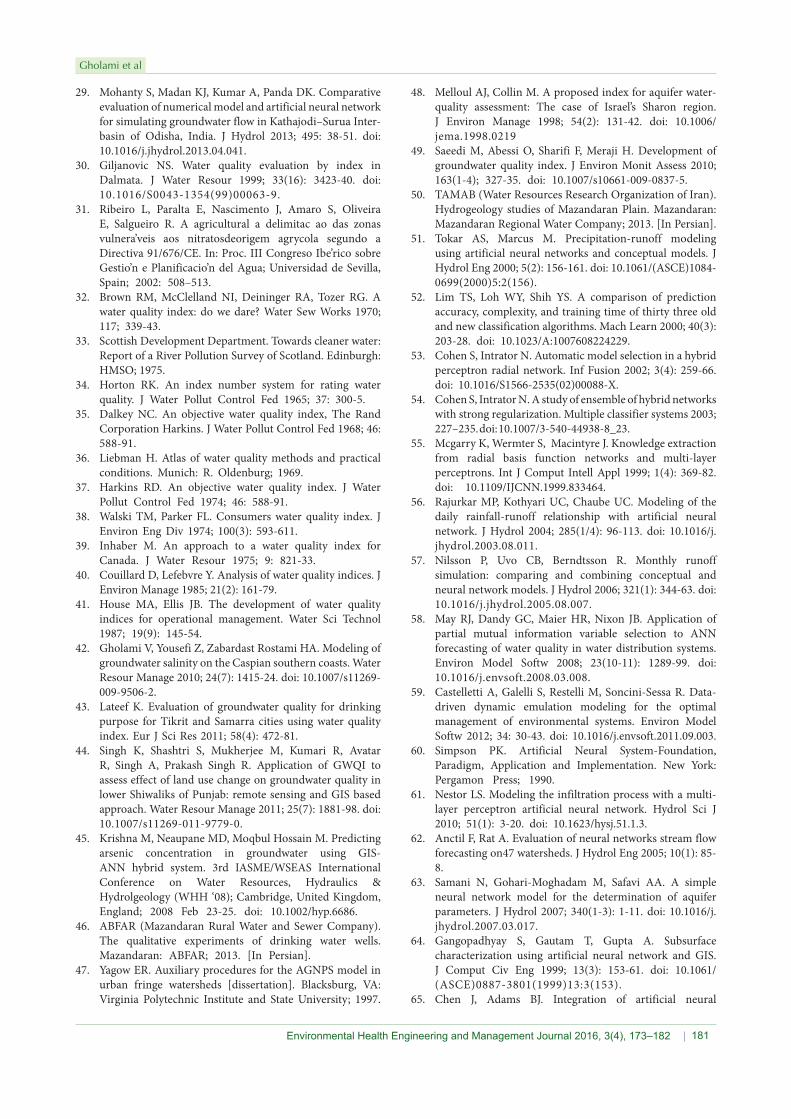
results in the training stage. Optimum network structure in groundwater quality simulation included a MLP with three inputs, tangent hyperbolic transfer function, LM (Levenberg-Marquart) training technique and one neu-ron. One of the best selections in modeling of hydrologic parameters are tangent hyperbolic transfer function and LM training technique and were employed in several studies as a prior selection in the world (62). After opti-mizing network, testing stage or efficiency evaluation is performed. Evaluation of ANN efficiency in groundwa-ter quality simulation, via comparison between estimated and actual GWQI values, in the validation (testing) stage is shown in Figure 8 (R2=0.73). According to the results, ANN can simulate GWQI with an acceptable accuracy. ANN capability in similar modelling is validated by previ-ous studies (63). The objective of this study is to estimate groundwater quality in sites without water quality data and also to preset the result in a manner that can be usable for all users.In GIS, raster layers of the three input factors were com-bined using overlay analysis with a pixel size 1×1 km. Pix-els data (network inputs and coordinate) were exported from GIS and then imported into Neuro Solutions soft-ware. In ANN medium, GWQI was simulated using the validated optimum network for all of the study plain. In the next step, simulated GWQI were imported from ANN to GIS medium with geographic location data (X, Y). GWQI values throughout the geographic coordinate and

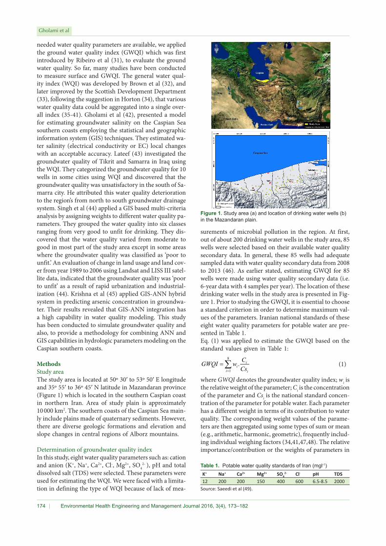
Figure 6. The map of distance from contaminant centers in the study area (m).

Figure 8. Evaluation of ANN efficiency in groundwater quality simulation. Comparison between the estimated and actual GWQI values in the validation (testing) stage (R2 = 0.73).

Figure 7. Evaluation of ANN efficiency in groundwater quality simulation in the training stage throughout the comparison between the estimated and actual GWQI values (R2 = 0.95).

Table 4. The results of network training for simulating GWQI

All runs Training minimum

Training SD

Cross validation minimum

Cross validation SD

Average of minimum MSEs 0.006 0.001 0.008 0.001Average of final MSEs 0.006 0.001 0.024 0.014

Table 5. The results of network training and optimum network selection

Best networks Training Cross validationEpoch # 1000 11Minimum MSE 0.005 0.006Final MSE 0.005 0.016

GIS capabilities were generated on groundwater quality map for study plain. Groundwater quality maps are shown in Figures 9 and 10. As can be seen, GWQI actual values were overlain on the generated GWQI map in GIS. We can evaluate result accuracy by overlaying actual values on the generated map. Results revealed that the estimated GWQI has a suitable accuracy and the results can be particularly employed in classifying ground water quality. Compari-son between water quality zones and estimated GWQI values showed the efficiency and accuracy of the integra-tion of ANN and GIS in modeling (45,64). GWQI values are classified into three categories; high (GWQI>0.15), low (GWQI<0.04), and suitable (0.04<GWQI <0.15) (49). As can be seen in Figures 9 and 10, the presented meth-odology can accurately simulate groundwater quality for ground water classification and existing error values does not flaw in the accuracy of water quality classification in the surface of a plain or a watershed. The actual GWQI values of 85 drinking water wells were overlain on the gen-erated raster layer of GWQI in GIS and the result accu-racy was evaluated via comparison between the simulated GWQI and the actual GWQI in GIS. Evaluation results showed that the results were accurate and acceptable. Fi-nally, the GWQI raster layer was presented after the clas-sification of the groundwater quality map.

DiscussionEight model structures were developed to evaluate the probability impacts of enabling/disabling transmissivity of aquifer formation, water table depth, the distance from contaminant centers, elevation, number of household and population as inputs. Results showed that three fac-tors, viz; transmissivity of aquifer formation, water table depth, and the distance from contaminant centers, are the


Gholami et al

most important factors and the best inputs for ground-water quality modeling (42). ANN is an efficient tool in modeling but, its results cannot be preset in the forms of maps and geo-referenced data. We applied ANN in simu-lating groundwater quality and GIS as a pre-processing and post-processing tool in the result monitoring and mapping. Also, GIS resulted in an increasing modeling accuracy and modeling velocity. The best network struc-ture in groundwater quality simulation was a MLP net-work with tangent hyperbolic transfer function and LM training technique. Previous studies proved that an ANN with LM technique is an efficient structure in hydrological parameters simulation (65,66). Based on the results of the training stage, mean square error (MSE) and coefficient of determination (R2) measures were 0.01 and 0.9 respective-ly. In the cross validation stage, mean MSE was 0.016. Fur-thermore, the results revealed that the best performance for LM algorithm was produced by the network. Using ANN for hydrologic parameters simulation followed good results in the past and, in most cases, there have been high correlation between simulated and observed hydrographs (67-69). Litta et al (70) developed ANN model with LM algorithm to derive thunderstorm forecasts from 1 to 24 ahead at Kolkata. In the testing stage, MSE and coeffi-cient of determination (R2) measures were 0.0005 and 0.73 respectively. The basis of the present study is automatic relation between ANN and GIS in modeling and mapping of results. Also, the results should have capability of over-lay analysis with other digital data. GIS can provide a high volume of input data within a short time and ANN can simulate hydrologic parameters for the sites without water quality data within a short time. Finally, the integration of ANN and GIS can present results in a manner of digital maps. The groundwater quality maps indicated that the quality of groundwater is improper in terms of potable water quality standards of Iran in most of the study plain. It is necessary to plan to conserve and optimize usage of water resources. Unfortunately, the quantitative data of network inputs (transmissivity, groundwater table depth and distance from contaminant centers of settlements and manufacture) are available in the Mazandaran plain. Therefore, we can apply the current methodology or simi-

lar methods in the surface of Mazandaran plain.

ConclusionResults evidently revealed that the ANNs are capable of modeling the groundwater quality. This, therefore, sub-stantiate the general enhancement achieved by using neu-ral networks in several other hydrological fields (12). Re-sults of the sensitivity analysis (input factors in network) showed that the most important factors for consideration in water quality are the water table depth, kind of aquifer formation and distance from contaminant centers. Pollu-tion is higher in coastal areas than in other areas as a result of high water table, alluvial sediment existence, popula-tion density and upstream watershed flow (71). Therefore, we should focus to plan water quality management in the coastal area. However, this methodology (ANN and GIS integration) can be applied for modeling in other qualita-tive indices. It is clear that we could select a smaller pixel size that produces a more accurate input about distance from contaminant centers however, a great number of in-put pixels accompany a limitation for simulation in ANN medium (ANN software). Also, we have not accessed the precise data in two main inputs, namely, groundwater ta-ble depth and transmissivity of aquifer formation. ANN can be an efficient tool in hydrologic parameters simula-tion using suitable inputs and optimum network struc-ture. Also, GIS is an efficient system in data processing and mapping. Coupling ANN with GIS capabilities could provide practitioners with easily interpretable water qual-ity maps in the management of these resources. Therefore, the presented methodology and other groundwater mod-els can be used for prospective planning of sustainable groundwater development and management of ground-water resources.

Acknowledgments We thank ABFAR (Mazandaran Rural Water and Sewer Company) for providing the groundwater quality second-ary data and for helping us with data pre-processing.

Ethical issuesThere were no ethical issues for writing of this article.

Figure 9. The map of groundwater quality (GWQI) obtained from ANN and GIS capabilities (the west of study plain). In this map, an evaluation of the results accuracy was done using a comparison between the simulated GWQI values with the actual GWQI values.

Figure 10. The map of groundwater quality (GWQI) resulted by ANN and GIS capabilities (the east of study plain). In this map, an evaluation of the results accuracy was done using a comparison between the simulated GWQI values with the actual GWQI values.

Gholami et al


Competing interestsWe affirm that this article is the original work of the au-thors and have no conflict of interest to declare.

Authors’ contributionsAll authors were involved in all stages of the article. On behalf of the co-authors, the corresponding author bears full responsibility for this submission.

References1. Maier HR, Dandy GC. Understanding the behavior and

optimizing the performance of back-propagation neural networks: an empirical study. Envir Model Softw 1998; 13(2): 179-91.

2. Dawson CW, Wilby RL. Hydrological modeling using artificial neural networks. Prog Phys Geogr 2001; 25(1): 80-108. doi: 10.1177/030913330102500104.

3. Kalogirou SA. Artificial neural networks in renewable energy systems applications: a review. Renew Sustain Energy Rev 2001; 5(4): 373-401. doi: 10.1016/S1364-0321(01)00006-5.

4. Sharma N, Chaudhry KK, Chalapati-Rao CV. Vehicular pollution modeling using artificial neural network technique: a review. J Sci Ind Res 2005; 64(9): 637-47.

5. Ahmadi-Nedushan B, St-Hilaire A, Berube M, Robichaud E, Thiemonge N, Bobee B. A review of statistical methods for the evaluation of aquatic habitat suitability for in stream flow assessment. River Res Appl 2006; 22(5): 503-23. doi: 10.1002/rra.918.

6. Abrahart RJ, See LM, Dawson CW. Neural network hydroinformatics: maintaining scientific rigour, practical hydroinformatics. Berlin Heidelberg: Springer; 2008. p. 33-47. doi: 10.1007/978-3-540-79881-1_3.

7. Mellit A, Kalogirou SA, Hontoria L, Shaari S. Artificial intelligence techniques for sizing photovoltaic systems: a review. Renew Sustain Energy Rev 2009; 13(2): 406-19. doi: 10.1016/j.rser.2008.01.006.

8. Elshorbagy A, Corzo G, Srinivasulu S, Solomatine DP. Experimental investigation of the predictive capabilities of data driven modeling techniques in hydrology - part 1: concepts and methodology. Hydrol Earth Syst Sci 2010; 14: 1931-41. doi: 10.5194/hess-14-1931-2010.

9. Elshorbagy A, Corzo G, Srinivasulu S, Solomatine DP. Experimental investigation of the predictive capabilities of data driven modeling techniques in hydrology - part 2: application. Hydrol Earth Syst Sci 2010; 14: 1943-61. doi: 10.5194/hess-14-1931-2010.

10. Maier HR, Jain A, Dandy GC, Sudheer KP. Methods used for the development of neural networks for the prediction of water resource variables in river systems: current status and future directions. Environ Model Softw 2010; 25(8): 891-909. doi: 10.1016/j.envsoft.2010.02.003.

11. Abrahart RJ, Anctil F, Coulibaly P, Dawson CW, Mount NJ, See LM, et al. Two decades of anarchy? Emerging themes and outstanding challenges for neural network river forecasting. Prog Phys Geogr 2012; 36(4): 480-513. doi: 10.1177/0309133312444943.

12. Wu W, Dandy GC, Maier HR. Protocol for developing ANN models and its application to the assessment of the quality of the ANN model development process in drinking water quality modeling. Environ Model Softw 2014; 54: 108-27. doi: 10.1016/j.envsoft.2013.12.016.

13. Maier HR, Dandy GC. Neural networks for the prediction and forecasting of water resources variables: a review of modeling issues and applications. Environ Model Softw 2000; 15(1): 101-24. doi: 10.1016/S1364-8152(99)00007-9.

14. Hsu KL, Gupta HV, Sorooshian S. Artificial neural network modeling of the rainfall–runoff process. Water Resour Res 1995; 31(10): 2517-30. doi: 10.1029/95WR01955.

15. sik S, Kalin L, Schoonover J, Srivastava P, Lockaby BG. Modeling effects of changing land use/cover on daily stream flow: An artificial neural network and curve number based hybrid approach. J Hydrol 2013; 485: 103-12. doi: 10.1016/j.jhydrol.2012.08.032.

16. Coulibaly P, Anctil F, Aravena R, Bobee B. Artificial neural network modeling of water table depth fluctuations. Water Resour Res 2001; 37(4): 885-96. doi: 10.1029/2000WR900368.

17. Coppola EA, Rana AJ, Poulton MM, Szidarovszky F, Uhl VW. A neural network approach for predicting aquifer water level elevations. Ground Water 2005; 43(2): 231-41. doi: 10.1111/j.1745-6584.2005.0003.x.

18. Daliakopoulos IN, Coulibaly P, Tsanis IK. Groundwater level forecasting using artificial neural network. J Hydrol 2005; 309(1): 229-40. doi: 10.1016/j.jhydrol.2004.12.001.

19. Lallahem S, Mania J, Hani A, Najjar Y. On the use of neural networks to evaluate groundwater levels in fractured media. J Hydrol 2005; 307(1–4): 92–111. doi: 10.1016/j.jhydrol.2004.10.005.

20. Nayak PC, Rao YR, Sudheer KP. Groundwater level forecasting in a shallow aquifer using artificial neural network approach. Water Resour Manage 2006; 20: 77-90. doi: 10.1007/s11269-006-4007-z.

21. Uddameri V .Using statistical and artificial neural network models to forecast potentiometric levels at a deep well in South Texas. Environ Geol 2007; 51(8): 885-95. doi: 10.1007/s00254-006-0452-5.

22. Krishna B, Satyaji Rao YR, Vijaya T. Modeling groundwater levels in an urban coastal aquifer using artificial neural networks. Hydrol Proc 2008; 22(8): 1180-88. doi: 10.1002/hyp.6686.

23. Trichakis IC, Nikolos IK, Karatzas GP. Optimal selection of artificial neural network parameters for the prediction of a karstic aquifer’s response. Hydrol Proc 2009; 23(20): 2956-69. doi: 10.1002/hyp.7410.

24. Ghose DK, Panda SN, Swain PC. Prediction of water table depth in western region, Orissa using BPNN and RBFN neural networks. J Hydrol 2010; 394(3-4): 296-304. doi: 10.1016/j.jhydrol.2010.09.003.

25. Yoon H, Jun SC, Hyun Y, Bae GO, Lee KK. A comparative study of artificial neural networks and support vector machines for predicting groundwater levels in a coastal aquifer. J Hydrol 2011; 396(1): 128-38. doi: 10.1016/j.jhydrol.2010.11.002.

26. Adamowski J, Chan HF. A wavelet neural network conjunction model for groundwater level forecasting. J Hydrol 2011; 407: 28-40. doi: 10.1016/j.jhydrol.2011.06.013.

27. Li X, Shu L, Liu L, Yin D, Wen J. Sensitivity analysis of groundwater level in Jinci Spring Basin (China) based on artificial neural network modeling. Hydrogeol J 2012; 20(4): 727-38. doi: 10.1007/s10040-012-0843-5.

28. Nourani V, Baghanam AH, Vousoughi VD, Alami MT. Classification of groundwater level data using SOM to develop ANN-based forecasting model. Int J Soft Comput Eng 2012; 2(1): 2231-07.


Gholami et al

29. Mohanty S, Madan KJ, Kumar A, Panda DK. Comparative evaluation of numerical model and artificial neural network for simulating groundwater flow in Kathajodi–Surua Inter-basin of Odisha, India. J Hydrol 2013; 495: 38-51. doi: 10.1016/j.jhydrol.2013.04.041.

30. Giljanovic NS. Water quality evaluation by index in Dalmata. J Water Resour 1999; 33(16): 3423-40. doi: 10.1016/S0043-1354(99)00063-9.

31. Ribeiro L, Paralta E, Nascimento J, Amaro S, Oliveira E, Salgueiro R. A agricultural a delimitac ao das zonas vulnera’veis aos nitratosdeorigem agrycola segundo a Directiva 91/676/CE. In: Proc. III Congreso Ibe’rico sobre Gestio’n e Planificacio’n del Agua; Universidad de Sevilla, Spain; 2002: 508–513.

32. Brown RM, McClelland NI, Deininger RA, Tozer RG. A water quality index: do we dare? Water Sew Works 1970; 117; 339-43.

33. Scottish Development Department. Towards cleaner water: Report of a River Pollution Survey of Scotland. Edinburgh: HMSO; 1975.

34. Horton RK. An index number system for rating water quality. J Water Pollut Control Fed 1965; 37: 300-5.

35. Dalkey NC. An objective water quality index, The Rand Corporation Harkins. J Water Pollut Control Fed 1968; 46: 588-91.

36. Liebman H. Atlas of water quality methods and practical conditions. Munich: R. Oldenburg; 1969.

37. Harkins RD. An objective water quality index. J Water Pollut Control Fed 1974; 46: 588-91.

38. Walski TM, Parker FL. Consumers water quality index. J Environ Eng Div 1974; 100(3): 593-611.

39. Inhaber M. An approach to a water quality index for Canada. J Water Resour 1975; 9: 821-33.

40. Couillard D, Lefebvre Y. Analysis of water quality indices. J Environ Manage 1985; 21(2): 161-79.

41. House MA, Ellis JB. The development of water quality indices for operational management. Water Sci Technol 1987; 19(9): 145-54.

42. Gholami V, Yousefi Z, Zabardast Rostami HA. Modeling of groundwater salinity on the Caspian southern coasts. Water Resour Manage 2010; 24(7): 1415-24. doi: 10.1007/s11269-009-9506-2.

43. Lateef K. Evaluation of groundwater quality for drinking purpose for Tikrit and Samarra cities using water quality index. Eur J Sci Res 2011; 58(4): 472-81.

44. Singh K, Shashtri S, Mukherjee M, Kumari R, Avatar R, Singh A, Prakash Singh R. Application of GWQI to assess effect of land use change on groundwater quality in lower Shiwaliks of Punjab: remote sensing and GIS based approach. Water Resour Manage 2011; 25(7): 1881-98. doi: 10.1007/s11269-011-9779-0.

45. Krishna M, Neaupane MD, Moqbul Hossain M. Predicting arsenic concentration in groundwater using GIS-ANN hybrid system. 3rd IASME/WSEAS International Conference on Water Resources, Hydraulics & Hydrolgeology (WHH ‘08); Cambridge, United Kingdom, England; 2008 Feb 23-25. doi: 10.1002/hyp.6686.

46. ABFAR (Mazandaran Rural Water and Sewer Company). The qualitative experiments of drinking water wells. Mazandaran: ABFAR; 2013. [In Persian].

47. Yagow ER. Auxiliary procedures for the AGNPS model in urban fringe watersheds [dissertation]. Blacksburg, VA: Virginia Polytechnic Institute and State University; 1997.

48. Melloul AJ, Collin M. A proposed index for aquifer water-quality assessment: The case of Israel’s Sharon region. J Environ Manage 1998; 54(2): 131-42. doi: 10.1006/jema.1998.0219

49. Saeedi M, Abessi O, Sharifi F, Meraji H. Development of groundwater quality index. J Environ Monit Assess 2010; 163(1-4); 327-35. doi: 10.1007/s10661-009-0837-5.

50. TAMAB (Water Resources Research Organization of Iran). Hydrogeology studies of Mazandaran Plain. Mazandaran: Mazandaran Regional Water Company; 2013. [In Persian].

51. Tokar AS, Marcus M. Precipitation-runoff modeling using artificial neural networks and conceptual models. J Hydrol Eng 2000; 5(2): 156-161. doi: 10.1061/(ASCE)1084-0699(2000)5:2(156).

52. Lim TS, Loh WY, Shih YS. A comparison of prediction accuracy, complexity, and training time of thirty three old and new classification algorithms. Mach Learn 2000; 40(3): 203-28. doi: 10.1023/A:1007608224229.

53. Cohen S, Intrator N. Automatic model selection in a hybrid perceptron radial network. Inf Fusion 2002; 3(4): 259-66. doi: 10.1016/S1566-2535(02)00088-X.

54. Cohen S, Intrator N. A study of ensemble of hybrid networks with strong regularization. Multiple classifier systems 2003; 227–235. doi: 10.1007/3-540-44938-8_23.

55. Mcgarry K, Wermter S, Macintyre J. Knowledge extraction from radial basis function networks and multi-layer perceptrons. Int J Comput Intell Appl 1999; 1(4): 369-82. doi: 10.1109/IJCNN.1999.833464.

56. Rajurkar MP, Kothyari UC, Chaube UC. Modeling of the daily rainfall-runoff relationship with artificial neural network. J Hydrol 2004; 285(1/4): 96-113. doi: 10.1016/j.jhydrol.2003.08.011.

57. Nilsson P, Uvo CB, Berndtsson R. Monthly runoff simulation: comparing and combining conceptual and neural network models. J Hydrol 2006; 321(1): 344-63. doi: 10.1016/j.jhydrol.2005.08.007.

58. May RJ, Dandy GC, Maier HR, Nixon JB. Application of partial mutual information variable selection to ANN forecasting of water quality in water distribution systems. Environ Model Softw 2008; 23(10-11): 1289-99. doi: 10.1016/j.envsoft.2008.03.008.

59. Castelletti A, Galelli S, Restelli M, Soncini-Sessa R. Data-driven dynamic emulation modeling for the optimal management of environmental systems. Environ Model Softw 2012; 34: 30-43. doi: 10.1016/j.envsoft.2011.09.003.

60. Simpson PK. Artificial Neural System-Foundation, Paradigm, Application and Implementation. New York: Pergamon Press; 1990.

61. Nestor LS. Modeling the infiltration process with a multi-layer perceptron artificial neural network. Hydrol Sci J 2010; 51(1): 3-20. doi: 10.1623/hysj.51.1.3.

62. Anctil F, Rat A. Evaluation of neural networks stream flow forecasting on47 watersheds. J Hydrol Eng 2005; 10(1): 85-8.

63. Samani N, Gohari-Moghadam M, Safavi AA. A simple neural network model for the determination of aquifer parameters. J Hydrol 2007; 340(1-3): 1-11. doi: 10.1016/j.jhydrol.2007.03.017.

64. Gangopadhyay S, Gautam T, Gupta A. Subsurface characterization using artificial neural network and GIS. J Comput Civ Eng 1999; 13(3): 153-61. doi: 10.1061/(ASCE)0887-3801(1999)13:3(153).

65. Chen J, Adams BJ. Integration of artificial neural

Gholami et al


networks with conceptual models in rainfall – runoff modeling, J Hydrol 2006; 318(1-4): 232-49. doi: 10.1016/j.jhydrol.2005.06.017.

66. Nayebi M, Khalili D. Daily stream flow predication capability of artificial neural networks as influenced by minimum air temperature data. Biosystems Engineering 2006; 95(4): 557-67. doi: 10.1016/j.biosystemseng.2006.08.012.

67. Crawford NH, Linsley RK. Digital simulation in hydrology: Stanford watershed model IV, technical report 10. Stanford, CA: Stanford University; 1966.

68. Chang FJ, Chang LC, Huang HL. Real-time recurrent learning neural network for stream-flow forecasting. Hydrol Proc 2002; 16(13): 2577-88. doi: 10.1002/hyp.1015.

69. Olsson J, Uvo CB, Jinno K, Kawamura A, Nishiyama K, Koreeda N, et al. Neural networks for rainfall forecasting by atmospheric downscaling. J Hydrol Eng 2004; 9(1): 1-12. doi: 10.1061/(ASCE)1084-0699(2004)9:1(1).

70. Litta AJ, Idicula SM, Mohanty UC. Artificial neural network model in prediction of meteorological parameters during Premonsoon thunderstorms. Int J Atmos Sci 2013; 2013: 525383. doi: 10.1155/2013/525383.

71. Gholami V, Aghagoli H, Kalteh AM. Modeling sanitary boundaries of drinking water wells on the Caspian Sea southern coasts, Iran. Environ Earth Sci 2015; 74(4): 2981-90. doi: 10.1007/s12665-015-4329-3.

Documents

Integration of artificial neural network and geographic