INTEGRATING GRADIENT SEARCH, LOGISTIC REGRESSION AND

Received 7 June 2012

Accepted 17 June 2013

INTEGRATING GRADIENT SEARCH, LOGISTIC REGRESSION ANDARTIFICIAL NEURAL NETWORK FOR PROFIT BASED UNIT

COMMITMENT

A.AmudhaResearch Scholar, Department of EEE, Anna University, Tiruchirappalli – 620 024

+91-044-24502430, +91-044-24501270, E-mail: [email protected]

C.Christober Asir RajanAssociate Professor, Department of EEE, Pondicherry Engineering College, Pondicherry – 605 014

+91-0413-2655281, +91-0413-2655101, E-mail: [email protected]

Abstract

As the electrical industry restructures many of the traditional algorithms for controlling generating units, they needeither modification or replacement. In the past, utilities had to produce power to satisfy their customers with theobjective to minimize costs and actual demand/reserve were met. But it is not necessary in a restructured system.The main objective of restructured system is to maximize its own profit without the responsibility of satisfying theforecasted demand. The Profit Based Unit Commitment (PBUC) is a highly dimensional mixed-integeroptimization problem, which might be very difficult to solve. Hence integrating Optimization Technique GradientSearch (GS), Logistic Regression (LR) and Artificial Neural Network (ANN) approach is introduced in this paperconsidering power and reserve generating in order to receive the maximum profit in three and ten unit system byconsidering the softer demand. Also this method gives an idea regarding how much power and reserve should besold in markets. The proposed approach has been tested on a power system with 3 and 10 generating units.Simulation results of the proposed approach have been compared with the existing methods. It is observed that theproposed algorithm provides maximum profit compared to existing methods.

Keywords: Artificial neural network, Competitive environment, Deregulation, Gradient search, LogisticRegression, Profit Based Unit Commitment, Restructured system

1. Introduction

Power Industry is undergoing restructuring throughoutthe world. The past decade has seen a dramatic changein the manner in which the power industry is organized.It has moved from a formally vertically integrated andhighly regulated industry to one that has beenhorizontally integrated in which generation,transmission and distribution are unbundled.

The basic aim of GENCOs (Generating Company) inrestructuring of power system is to create competitionamong generating companies and provide choice ofdifferent generation options at a competitive price toconsumers. The main objective of GENCOs is tomaximize their own profit by considering the softerdemand. In the past, utilities had to produce power tosatisfy their customers with the minimum production

International Journal of Computational Intelligence Systems, Vol. 7, No. 1 (February 2014), 90-104

Co-published by Atlantis Press and Taylor & FrancisCopyright: the authors

90

cost. This means utilities run Unit Commitment (UC)with the condition that demand and reserve must bemet.

In this paper, the authors intend to explain theimportance of open market environment to GENCOthat gives an idea for power producers to maximizetheir own profit as well as to maintain the power qualityto consumers. Because of the fast economicdevelopment, the electricity demand is growing rapidlyand the power system expansion becomes a severeeconomic burden of the government and a bottleneck ofoverall economy sustainable development.

It is urgent to launch power system restructuring andderegulation and to establish power markets with faircompetition so as to attract more investments fromvarious sources to power industry. In [2] it isimpossible to predict the future UC scheduling, butwith the Genetic Based Unit Commitment Algorithm(GBUCA) ability, good UC schedules and reasonablecomputer execution time using the true costingapproach can be obtained The authors have reportedresearch illustrating how power producers makedecisions when having the option of selling to both thespot power market and reserve market [3]. GBUCAwas updated for the PBUC-GA and to provide the userwith additional information that identifies whichschedules ,allow the user more market flexibility forgiven level of profit [4]. But disadvantages of the GAsolution for PBUC problem are that the final solutionbeing heuristic in nature may not be satisfactory. In [7]the author gives an overview of concept of UC problemwith a bibliographical survey of relevant back ground,and provides a representative sample of currentengineering thinking pertaining to the next generationUC problem. Hybrid method LR-EP has been used forsolving the PBUC problem due to their ability to solvePBUC problems more efficiently [6], [15].

PBUC problems were solved by using conventionalmethods such as Dynamic Programming (DP) andLagrange Relaxation (LR) methods [10] previously.Due to the curse of dimensionality with increase innumber of generating units, LR method suffers fromnumerical convergence and DP method takes hugecomputational time to obtain an optimal solution. TheMuller method was introduced to solve economic

dispatch problem and Improved Pre- prepared PowerDemand Table was introduced to solve combinatorialsub problem for deregulated environment without theeffect of r where r is the probability that the reserve iscalled and generated [11].

The formulation in [12 profitbased on the forecasted Locational Marginal Prices(LMPs). In paper [13], price uncertainty is modeled in aprocedure using fuzzy members for maximizing aGENCO 4], the formulation andsolution of security constrained unit commitment solvessimultaneous optimization of energy and ancillaryservices markets. In paper [16], a methodology isproposed for managing risks faced by power producerstrading in energy market a day ahead. In paper [17],Quantum-Inspired Evolutionary Algorithm (QEA) isapplied to solve the UC problem and proposes novelQEA-based UC method (QEA-UC) in which the unit-scheduling problem is handled by QEA and theeconomic dispatch problem is solved by the commonly-used method, Lambda-Iteration Technique. The authorin paper [18] investigates modeling approaches for thecomputational cost reduction of Stochastic UCformulations. Long term UCP was considered withoutramp rate limit constraints of individual units [19]. In

paper [20] ,Quantum Inspired Binary Particle SwarmOptimization (QBPSO) is based on the concept andprinciples of quantum computing and developed toenhance the conventional Binary Particle SwarmOptimization(BPSO)in solving the combinatorialoptimization problems. In paper [21], Transmissionswitching (TS) was integrated with UC for solving themulti interval optimal generation unit scheduling withsecurity constraints .Hybrid Particle SwarmOptimization (HPSO) which is a blend of BPSO andReal Coded particle Swarm Optimization (RCPSO)isproposed in [22]. The UC problem is handled by BPSO,while RCPSO solves the economic load dispatchproblem. Both algorithms run simultaneously, adjustingtheir solutions in search of a better solution..From the literature survey, it is observed that most ofthe existing algorithms have some limitations toprovide the qualitative solution. The proposed methodconsiders both power and reserve generation at thesame time. This paper is organized as follows: Part IIbriefly describes the UC problem formulation and


91

highlights modification needed for the competitiveenvironment. Part III explains the market structure ofselling power and energy. Part IV discusses thefundamentals of Gradient Search (GS), LogisticRegression (LR) and Artificial Neural Network (ANN)and its implication on PBUC. Finally, part V providesconclusion and future scope of the work.

2. Problem Formulation

The objective of UC is not to minimize costs as beforebut to provide the maximum profit for a company. It isan optimization problem and can be formulatedmathematically by the following equations.The Objective function is

.MaxP F TC(1)

(or)MinTC RV

(2)

Subject to

TtDXP t

N

iitit ...........1,'

1

(3)

TtSRXR t

N

iitit ...........1,'

1

(4)

Redefining the UC problem for the competitiveenvironment involves changing the demand and reserveconstraints from an equality to less than or equal to theforecasted level if it creates more profit.

maxmin iii PPP (5)

minmax0 iii PPR (6)

maxiii PPR (7)

Minimum Up and Downtime constraints: wherevariables are defined as follows:

PF profit of Genco ;RV revenue of Genco ;TC total cost of Genco ;Pit power generation of generator at hour t;

Rit reserve generation of generator at time t;Xit on/off status of generator at hour t;

D’t forecasted demand at hour t;SR’t forecasted reserve at hour t;Pi min minimum generation limit of generator i ;Pi max maximum generation limit of generator I;N number of generator units;T number of hours;Here forecasted demand, reserve and prices areimportant inputs to the PBUC algorithm; they are usedto determine the expected revenue (1), which affects theexpected profit.

3. Power producer Strategies for selling power and

reserve

If a power producer is able to sell power in to a reserve

maximization in both the spot and reserve markets areintertwined. The producer decides to pi (S) in the spotmarket and Pi(R) in the reserve market. The exactdetermination of Pi (S) & Pi(R) depends on the wayreserve payments are made, although results are verysimilar. (3)

3.1 Payment for Power Delivered

In this method, the reserve is paid when only it isactually used. Therefore, the reserve price is higher thanthe power (spot) price. Revenue and cost in ( 1) can becalculated from

(8)

(9)

WhereSPt -forecasted Spot price at hour tRPt - forecasted reserve price at hour tFi -fuel cost function of generator iST - start up cost.r- probability that the reserve is called and generated

3.2 Payment for reserve allocatedIn this method, GENCO receives the reserve price perunit of reserve for every time period that the reserve isallocated and not used. When the reserve is used,

it

N

i

T

tititit

N

i

T

titit XSTXRPFrXPFrTC ...1

1 11 1

N

i

T

titittit

N

i

T

ttit XRRPrXSPPRV

1 11 1

....


92

GENCO receives the spot price for the reserve that isgenerated. In this method, reserve price is much lowerthan the spot price. Revenue and costs in (1) can becalculated from.

(10)

(11)

Where

F (Pit)expressed as ai + bi pit + ci pit

2 in which ai, bi and ci are

4. Proposed Methodology

The proposed methodology deals with solving the UCproblem in a fitting way than all the previous methodsdefined for the same cause. Gradient Descent (GD)proves to be the best possible machine learningoptimization available to determine the global minimaof a particular function. Similarly Logistic regression isthe recent and most efficient technique in predicting theBest Fit among binary status options, generator on/offstatus in this case, using a predefined criterion or atraining data set. The hybrid obtained between thesetechniques applies state of the act machine learningtechniques to the unit commitment problem.Gradient Descent (GD) is a met heuristic optimizationalgorithm used to obtain the global or near globalminimum of most functions. Gradient descent is basedon the observation that if the multivariable function isdefined F(x) and differentiable in a neighborhood of apoint a, then ( )F x decreases very fast if one goesfrom a in the direction of the negative gradient of F ata.For 0α a small enough number, then

( ) ( )F a F b . With this observation in mind, onestarts with a guess x0 for a local minimum of F, andconsiders the sequence x0,x1,x2…such thatxn+1 = xn

n where

We have

10 2( ) ( ) ( )F X F X F X

so hopefully the sequence (xn) converges to the desiredlocal minimum. Note that the value of the step size γ isallowed to change in each iteration Here F is assumedto be defined on the plane, and that its graph has a bowlshape. The blue curves are the contour lines, that is, theregions on which the value of F is constant. A redarrow originating at a point shows the direction of thenegative gradient at that point. Note that the (negative)gradient at a point is orthogonal to the contour linegoing through that point. We see that gradient descentleads us to the bottom of the bowl, that is, to the pointwhere the value of the function F is minimal.Logistic regression (LR) is used for prediction of theprobability of occurrence of an event by fitting data to alogistic function. It is a generalized linear model usedfor binomial regression. Like other forms of regressionanalysis, it makes use of one or more predictorvariables that may be either numerical or categorical.The logistic function used in solving logistic regression

is, Whereze

Zf1

1(12)

z is the input to the sigmoid function, Xz Tθx is the input to the logistic regression classifier.f (z) is the event probability.

The function is sometimes called sigmoid function andit takes the values between 0 and1. Therefore it predictsonly the probability of the event happening. Thus it is asuitable tool for solving the on\off criterion based onthe constraints.An artificial neural network (ANN), usually calledneural network (NN), is a mathematical model orcomputational model that is inspired by the structureand/or functional aspects of biological neural networks.A neural network consists of an interconnected group ofartificial neurons, and it processes information using aconnectionist approach to computation. In most casesan ANN is an adaptive system that changes its structurebased on external or internal information that flowsthrough the network during the learning phase. Modernneural networks are non-linear statistical data modelingtools. They are usually used to model complexrelationships between inputs and outputs or to findpatterns in data.

N

i

T

tititttit

N

i

T

ttit XRSPrRPrXSPPRV

1 11 1

..1..

it

N

i

T

tititit

N

i

T

titit XSTXRPFrXPFrTC ...1

1 11 1


93

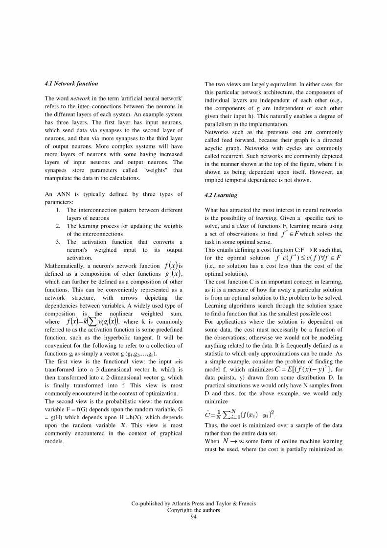
4.1 Network function

The word network in the term 'artificial neural network'refers to the inter connections between the neurons inthe different layers of each system. An example systemhas three layers. The first layer has input neurons,which send data via synapses to the second layer ofneurons, and then via more synapses to the third layerof output neurons. More complex systems will havemore layers of neurons with some having increasedlayers of input neurons and output neurons. Thesynapses store parameters called "weights" thatmanipulate the data in the calculations.

An ANN is typically defined by three types ofparameters:

1. The interconnection pattern between differentlayers of neurons

2. The learning process for updating the weightsof the interconnections

3. The activation function that converts aneuron's weighted input to its outputactivation.

Mathematically, a neuron's network function xf isdefined as a composition of other functions xgi ,which can further be defined as a composition of otherfunctions. This can be conveniently represented as anetwork structure, with arrows depicting thedependencies between variables. A widely used type ofcomposition is the nonlinear weighted sum,where xgwkxf iii , where k is commonlyreferred to as the activation function is some predefinedfunction, such as the hyperbolic tangent. It will beconvenient for the following to refer to a collection offunctions gi as simply a vector g (g1,g2 n).The first view is the functional view: the input istransformed into a 3-dimensional vector h, which isthen transformed into a 2-dimensional vector g, whichis finally transformed into f. This view is mostcommonly encountered in the context of optimization.The second view is the probabilistic view: the randomvariable F = f(G) depends upon the random variable, G= g(H) which depends upon H =h(X), which dependsupon the random variable . This view is mostcommonly encountered in the context of graphicalmodels.

The two views are largely equivalent. In either case, forthis particular network architecture, the components ofindividual layers are independent of each other (e.g.,the components of g are independent of each othergiven their input h). This naturally enables a degree ofparallelism in the implementation.Networks such as the previous one are commonlycalled feed forward, because their graph is a directedacyclic graph. Networks with cycles are commonlycalled recurrent. Such networks are commonly depictedin the manner shown at the top of the figure, where f isshown as being dependent upon itself. However, animplied temporal dependence is not shown.

4.2 Learning

What has attracted the most interest in neural networksis the possibility of learning. Given a specific task tosolve, and a class of functions F, learning means usinga set of observations to find Ff * which solves thetask in some optimal sense.This entails defining a cost function C:F R such that,for the optimal solution ( ) ( )f c f c f f F(i.e., no solution has a cost less than the cost of theoptimal solution).The cost function C is an important concept in learning,as it is a measure of how far away a particular solutionis from an optimal solution to the problem to be solved.Learning algorithms search through the solution spaceto find a function that has the smallest possible cost.For applications where the solution is dependent onsome data, the cost must necessarily be a function ofthe observations; otherwise we would not be modelinganything related to the data. It is frequently defined as astatistic to which only approximations can be made. Asa simple example, consider the problem of finding themodel f, which minimizes 2[( ( ) ) ]C E f x y , fordata pairs(x, y) drawn from some distribution D. Inpractical situations we would only have N samples fromD and thus, for the above example, we would onlyminimize

.Thus, the cost is minimized over a sample of the datarather than the entire data set.When N some form of online machine learningmust be used, where the cost is partially minimized as


94

each new example is seen. While online machinelearning is often used when is fixed, it is most usefulin the case where the distribution changes slowly overtime. In neural network methods, some form of onlinemachine learning is frequently used for finite datasets.

4.3 Hybrid between GD-LR using ANN

This method first involves the determination ofminimum fuel cost of each generator from the functiondefined (1) using gradient descent. Next the powercorresponding to the minimum fuel cost is determined.If Pmincost<Pmin Pmincost=Pmin

If Pmincost>Pmax Pmincost=Pmax

Then the dataset consisting of all the power values at anincrement of one unit from Pmincost to Dt

This dataset is fed to the logistic regression classifier.The logistic regression is already trained with aclassifier dataset obtained by applying the requiredconstraints to the available dataset. Thus the classifier istrained to a parameter set θ which is obtained byminimizing the cost function,

( ) ( ) ( )( )

1

1( ) [ log( ( ) (1 ) log(1 ( )]

i i im

ie e

i

J Y h X y h xm

θ(13)

Wherey(i) status of generator i corresponding to thePmincost

h (x(i)) Predicted status of generator i for supplyingthe entire forecasted demand.(subject to sigmoidfunction in equation 3)m product of total number of generators andnumber of hours

cost function

This parameter set theta is multiplied to the inputforecasted power and the status of the generatorcorresponding to the hour of demand is found byfeeding it to the sigmoid function as described by (12).This output of the sigmoid function is deciphered as,Xit = 1 if f(zit)Xit = 0 if f(zit) < 0.5WhereXit is the on/off status of generator described inEquations (8) and (9).

f(zit) is the predicted probability of the generator beingturned ON which is the output of logistic regressionclassifier.The value of 0.5 is decided assuming zero biasconditions of generators. But they can be redefined tovarious values depending on the precision and recallvalues.

This on/off status uses an artificial neural network todecide the power limit between switching on a newgenerator. This dynamic power varies as a function ofthe forecasted demand. This demand if exceeds theparticular limit as set by the ANN, the next generatorstatus is turned to ON. It uses a single direction logic,multi- input forward backward prediction algorithm.The network has 6 inputs and a hidden layer of 6 unitsand one output unit which gives a dynamic value of thepower difference for each stage. The ANN isimplemented just once to make sure that computationaloverhead is avoided. The stage uses forecasted demandto predict the power difference for each stage which isfed to the logistic regression classifier for the predictionprocess. This constraint is a main factor in deciding theOn/Off status for the machine as this value is given avery high weightage is given to this parameter duringmean normalization. The cost function and networkparameters are as defined earlier.

The various inputs areforecasted demand (i)spot pricestart up costfuel costforecasted demand of previous hour (i-1)initial status

The output is the power difference for the current hour(i) which opens up the next generator. This neuralfunction aids the improvement of the reliability of thesystem and thus improving the efficiency to aconsiderably higher level than using a static predictionof data from forecasted demand. This On/off statusalong with the power dataset is fed to the total costfunction where the profit of each of the possiblecombination of power is calculated. The entire value isnegated and the global minimum of the function isdetermined using the gradient descent operation (whichis called gradient ascent). Thus the maximum value of


95

the profit obtained and the corresponding power arecalculated by the algorithm.The dataset used to train logistic regression isregenerated by the principle of symmetry subject to theconstraints. The main constraint that is maintained toimprove the profit is

Ton

Toff

This regeneration creates a huge dataset thus enablingthe better performance of the classifier. The generatorhas to be scheduled to generate its rated power at thehour it is marked on. Thus the up time is considered forthe process also. After the process is complete thegenerated power and the on/off status is supplied to thesame logistic regression classifier to check the reservegeneration of limit of each generator and the iterationprocess is repeated for reserve to find the reservegeneration ranging from 0 to SRt

the GENCO is calculated. The learning rate of theclassifier for the reserve power is maintained at arelatively less value to enable proper convergence ofmetaheuristic minimization technique.

ALGORITHM

1 Start the process2 Obtain the input data (number of generators, demandhours, forecasted demand and forecasted price)3 Check if the current time period exceeds the requireddemand period4 Find power corresponding to minimum cost of eachgenerator, by feeding the cost curve and a suitablelearning rate to the gradient descent algorithm5 By iterating from the value obtained in step 4 to themaximum limit, find all the possible values of profit insteps of one (assuming each generator is on)6 Find the maximum profit and the powercorresponding to it, by feeding the data input and thelearning rate to the gradient descent algorithm7 The minimum difference in power between thedemands for the generators to turn on is fixeddynamically for each generator by the ANN classifierwhich takes demand, fuel cost, profit and the demandsustenance (how much time the demand stays) given byTon >> Tstart, as input parameters

8 Feed the input data such as number of generators,demand, maximum and minimum limit, constraints,power difference from step 7 and others to the logisticregression classifier9 Multiply the output schedule of generators (binaryvalue (0, 1)) with the power obtained in step 6 and sumthem up to obtain the total power supplied10 Find the corresponding cost, revenue and profit11 Separate the reserve power if it gives better profit byiterating over the profit values for various combinations12 Stop when the process is complete for all thedemand hours5. Numerical Results

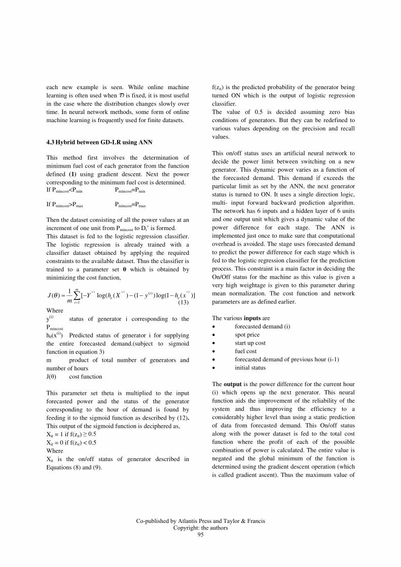
The proposed method has been implemented in Matlaband tested using two different systems to solve PBUCproblem. Before running PBUC-GS, LR and ANN, theGencos need to get an accurate hourly demand andprice forecast for the scheduling period. Fuel costfunction of each generator is estimated into quadraticform. Based on the forecasted information, power isdispatched economically by the proposed method.Simulations are carried out to find optimal solution, andprofit and they are also compared with existingmethods. The proposed method considers the effect ofprobability that reserve is called and generated for 3and 10 unit system. The forecasted demand, forecastedprices and fuel cost data of 3 unit system are listed inTableA1 and TableA2. In PBUC, Gencos no longerhave the obligation to meet the demand. Gencos maychoose to generate less than the demand.Three Unit SystemsThe effect of probability that reserve is called andgenerated (r) is tested using 3 generator 12 hour testdata. Here, reserve price is fixed at the triple and 0.01times of spot price for reserve payment method A andB, respectively, while is r varied from 0.005 to 0.05.Simulation results are shown in Tables I and II, and itis clear that profit obtained by method A is higher thanmethod B when r is varied. In method A, reserve is paidonly when the reserve power is actually delivered andused. Profit is more sensitive when r is varied.

The effect of reserve price is investigated in reservepayment method A and method B. In this case r is fixedat 0.005 while the reserve price is varied. From table IIIand table IV, it is observed that profit obtained by


96

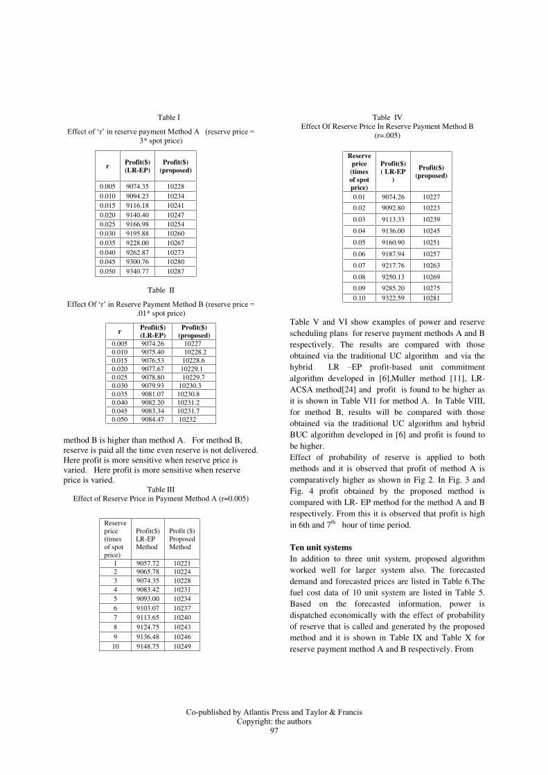
Table I

3* spot price)

Table II

.01* spot price)

r Profit($)(LR-EP)

Profit($)(proposed)

0.005 9074.26 102270.010 9075.40 10228.20.015 9076.53 10228.60.020 9077.67 10229.10.025 9078.80 10229.70.030 9079.93 10230.30.035 9081.07 10230.80.040 9082.20 10231.20.045 9083.34 10231.70.050 9084.47 10232

method B is higher than method A. For method B,reserve is paid all the time even reserve is not delivered.Here profit is more sensitive when reserve price isvaried. Here profit is more sensitive when reserveprice is varied.

Table IIIEffect of Reserve Price in Payment Method A (r=0.005)

Table IVEffect Of Reserve Price In Reserve Payment Method B

(r=.005)

Table V and VI show examples of power and reservescheduling plans for reserve payment methods A and Brespectively. The results are compared with thoseobtained via the traditional UC algorithm and via thehybrid LR EP profit-based unit commitmentalgorithm developed in [6],Muller method [11], LR-ACSA method[24] and profit is found to be higher asit is shown in Table VI1 for method A. In Table VIII,for method B, results will be compared with thoseobtained via the traditional UC algorithm and hybridBUC algorithm developed in [6] and profit is found tobe higher.Effect of probability of reserve is applied to bothmethods and it is observed that profit of method A iscomparatively higher as shown in Fig 2. In Fig. 3 andFig. 4 profit obtained by the proposed method iscompared with LR- EP method for the method A and Brespectively. From this it is observed that profit is highin 6th and 7th hour of time period.

Ten unit systemsIn addition to three unit system, proposed algorithmworked well for larger system also. The forecasteddemand and forecasted prices are listed in Table 6.Thefuel cost data of 10 unit system are listed in Table 5.Based on the forecasted information, power isdispatched economically with the effect of probabilityof reserve that is called and generated by the proposedmethod and it is shown in Table IX and Table X forreserve payment method A and B respectively. From

r Profit($)(LR-EP)

Profit($)(proposed)

0.005 9074.35 102280.010 9094.23 102340.015 9116.18 102410.020 9140.40 102470.025 9166.98 102540.030 9195.88 102600.035 9228.00 102670.040 9262.87 102730.045 9300.76 102800.050 9340.77 10287

Reserveprice(timesof spotprice)

Profit($)LR-EPMethod

Profit ($)ProposedMethod

1 9057.72 102212 9065.78 102243 9074.35 102284 9083.42 102315 9093.00 102346 9103.07 102377 9113.65 102408 9124.75 10243

9 9136.48 1024610 9148.75 10249

Reserveprice(timesof spotprice)

Profit($)( LR-EP

)

Profit($)(proposed)

0.01 9074.26 10227

0.02 9092.80 10223

0.03 9113.33 10239

0.04 9136.00 10245

0.05 9160.90 10251

0.06 9187.94 10257

0.07 9217.76 10263

0.08 9250.13 10269

0.09 9285.20 10275

0.10 9322.59 10281


97

Table VPower and reserve generation of reserve payment method A(r=.005, reserve price = 3* spot price)

Hour

PBUC by LR –EP[6]

Profit ($)

PBUC by GS,LR &ANN

Profit ($)Power (MW) Reserve (MW) Power (MW) Reserve (MW)

U1 U2 U3 U1 U2 U3 U1 U2 U3 U1 U2 U3

1 0 0 170 0 0 20 531.4 0 0 169.6 0 0 20 529.472 0 0 200 0 0 0 570 0 0 199.6 0 0 0 568.73 0 0 200 0 0 0 300 0 0 199.6 0 0 0 300.624 0 0 200 0 0 0 390 0 0 199.6 0 0 0 3905 0 379.9 200 0 20.1 0 201 0 399 200 0 0 0 501.256 0 400 200 0 0 0 1350 400 400 200 0 0 0 1829.017 0 400 200 0 0 0 1380 400 400 200 0 0 0 1878.978 0 400 200 0 0 0 990 0 399 200 0 0 0 1290.399 0 400 200 0 0 0 810 0 399 200 0 0 0 1110.79

10 0 130 200 0 35 0 818.1 0 329 0 0 35 0 686.8911 0 200 200 0 40 0 804.6 0 399 0 0 0 0 600.5212 0 350 200 0 50 0 829.2 0 399 0 0 0 0 540.82

9074.3 TOTAL 10,228

Table VIPower and reserve generation of reserve payment method B (r=.005, reserve price =.04 x spot price)

Hour

PBUC by LR –EP[6] PBUC by GS ,LR&ANN

Profit ($)Power (MW) Reserve (MW) Profit ($) Power (MW) Reserve (MW)

U1 U2 U3 U1 U2 U3 U1 U2 U3 U1 U2 U3

1 0 0 170 0 0 20 537.7 0 0 169.6 0 0 20 535.76

2 0 0 200 0 0 0 570 0 0 199.6 0 0 0 568.77

3 0 0 200 0 0 0 300 0 0 199.6 0 0 0 300.62

4 0 0 200 0 0 0 390 0 0 199.6 0 0 0 390

5 0 330 200 0 70 0 215.7 0 399 200 0 0 0 501

6 0 400 200 0 0 0 1350 400 400 200 0 0 0 1829

7 0 400 200 0 0 0 1380 400 400 200 0 0 0 1878.97

8 0 400 200 0 0 0 990 0 399 200 0 0 0 1290.39

9 0 387.2 200 0 12.8 0 810.4 0 399 200 0 0 0 1110.79

10 0 130 200 0 35 0 829.8 0 329 0 0 35 0 698.57

11 0 200 200 0 40 0 817.4 0 399 0 0 0 0 600.52

12 0 350 200 0 50 0 945.0 0 399 0 0 0 0 540.82

9136 TOTAL 10245

Table VIIComparison of the results of 3 unit system with existing

methods by proposed method (Method A)

Table VIIIComparison of the results of 3 unit system with existing

methods by proposed method (Method B)

S.no Method Profit ($)

1 Traditional UC[6] 4262.7

2 PBUC by LR-EP method [6] 9136.0

5 Proposed method 10245

S.no Method Profit ($)1 Traditional UC[6] 4048.82 PBUC by LR-EP method [6] 9074.33 PBUC by Muller method [11] 9030.54 PBUC by LR-ACSA method [24] 9081.15 Proposed method 0228


98

Fig 2. Effect of Probability of Reserve

Fig 3. Comparison of Profit between LR-EP & ProposedMethod A

Fig 4. Comparison of Profit between LR-EP & Proposed

Method B

Table XI, it is clear that the proposed method providesmaximum profit for method A compared to theexisting methods of PBUC by LR-EP method [6 ],Muller method [11], MAS [23 ], TS RP [26], TS IRP[ 26] and improved PSO [25] . For method B ,profitobtained by LR-EP method [6 ] is compared withproposed method as shown in Table XII.

6. Conclusion

In this paper, the authors have proposed an algorithm tosolve the PBUC for three and ten unit restructuredpower system. Based on forecasted demand, PBUC issolved with the effect of r. The effect of probability ofreserve and reserve power is considered for three unitsystem and two types of reserve payment methods aresimulated. All simulated results of three and ten unit

system are compared with results of existing methodsand it is observed that profit is obtained by the proposedmethod is higher. For further research, PBUC withtransmission losses and emission constraints will beconsidered. With these constraints added, the end usercan enjoy emission free economic power

Table XI

Comparison of the results of 10unit system (24Hr) withexisting methods by proposed methodA


1 PBUC by LR-EP method [6 ] 112818.93

2 PBUC by Muller method [11] 103296

3 PBUC MAS [ 23 ] 109485.19

4 PBUC by TS RP [26] 101086.

5 PBUC by TS IRP [ 26] 103261

6 PBUC by improved PSO [25] 113018.7


Table XII

Comparison of the results of 10unit system (24Hr) withexisting methods by proposed method B


2 PBUC by LR-EP method [6] 107838.58


TableA1 Forecasted Demand and Price for 3 Generator Case

HourForecasteddemand(MW)

Forecasted spotprice ($/MWH)

Forecastedreserve(MW)

1 170 10.55 20

2 250 10.3525

3 400 9.00 40

4 520 9.45 55

5 700 10.00 70

6 1050 11.25 95

7 1100 11.30 100

8 800 10.65 80

9 650 10.35 65

10 330 11.,20 35

11 400 10.75 40

12 550 10.60 55


99

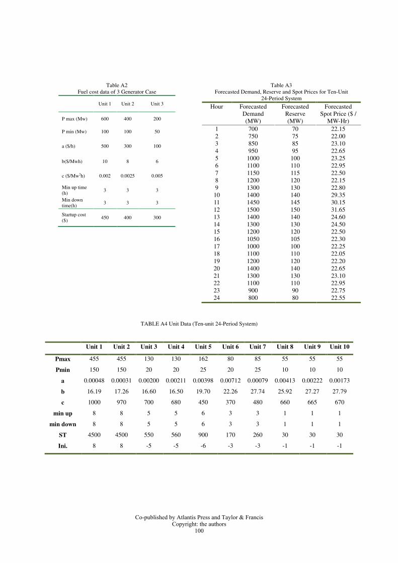
Table A2Fuel cost data of 3 Generator Case

Unit 1 Unit 2 Unit 3

P max (Mw) 600 400 200

P min (Mw) 100 100 50

a ($/h) 500 300 100

b($/Mwh) 10 8 6

c ($/Mw2h) 0.002 0.0025 0.005

Min up time(h)

3 3 3

Min downtime(h)

3 3 3

Startup cost($)

450 400 300

Table A3Forecasted Demand, Reserve and Spot Prices for Ten-Unit

24-Period System

Hour ForecastedDemand(MW)

ForecastedReserve(MW)

ForecastedSpot Price ($ /

MW-Hr)1 700 70 22.152 750 75 22.003 850 85 23.104 950 95 22.655 1000 100 23.256 1100 110 22.957 1150 115 22.508 1200 120 22.159 1300 130 22.80

10 1400 140 29.3511 1450 145 30.1512 1500 150 31.6513 1400 140 24.6014 1300 130 24.5015 1200 120 22.5016 1050 105 22.3017 1000 100 22.2518 1100 110 22.0519 1200 120 22.2020 1400 140 22.6521 1300 130 23.1022 1100 110 22.9523 900 90 22.7524 800 80 22.55

TABLE A4 Unit Data (Ten-unit 24-Period System)

Unit 1 Unit 2 Unit 3 Unit 4 Unit 5 Unit 6 Unit 7 Unit 8 Unit 9 Unit 10

Pmax 455 455 130 130 162 80 85 55 55 55

Pmin 150 150 20 20 25 20 25 10 10 10

a 0.00048 0.00031 0.00200 0.00211 0.00398 0.00712 0.00079 0.00413 0.00222 0.00173

b 16.19 17.26 16.60 16.50 19.70 22.26 27.74 25.92 27.27 27.79

c 1000 970 700 680 450 370 480 660 665 670

min up 8 8 5 5 6 3 3 1 1 1

min down 8 8 5 5 6 3 3 1 1 1

ST 4500 4500 550 560 900 170 260 30 30 30

Ini. 8 8 -5 -5 -6 -3 -3 -1 -1 -1


100

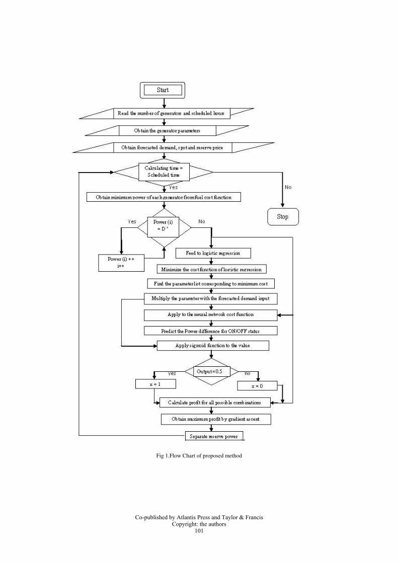
Fig 1.Flow Chart of proposed method


101

Table IXExample of power and Reserve generation of reserve payment method A (10 Units system)

(r=0.05, reserve price =5 X spot price)

Table XExample of power and Reserve generation of reserve payment method B (10 Units system)

(r=0. 05, reserve price = 0.01 X spot price)

Hr PBUC( method A)by proposed method

Power(MW) Reserve(MW) Profit $

U1 U2 U3 U4 U5 U6 U7 U8 U9 U10 U1 U2 U3 U4 U5 U6 U7 U8 U9 U10

1 345 354 0 0 0 0 0 0 0 0 0 70 0 0 0 0 0 0 0 0 3907.3

2 370 379 0 0 0 0 0 0 0 0 75 0 0 0 0 0 0 0 0 0 4076.3

3 420 429 0 0 0 0 0 0 0 0 0 0 0 0 0 0 0 0 0 0 5153.7

4 455 456 0 0 0 0 0 0 0 0 0 0 0 0 0 0 0 0 0 0 5127. 3

5 455 456 0 0 0 0 0 0 0 0 0 0 0 0 0 0 0 0 0 0 5673.3

6 455 456 0 0 0 0 0 0 0 0 0 0 0 0 0 0 0 0 0 0 5400.3

7 455 456 0 0 0 0 0 0 0 0 0 0 0 0 0 0 0 0 0 0 4990.8

8 455 456 0 0 0 0 0 0 0 0 0 0 0 0 0 0 0 0 0 0 4672.3

9 455 456 0 0 0 0 0 0 0 0 0 0 0 0 0 0 0 0 0 0 5263.8

10 455 456 0 0 0 0 0 56 0 0 0 0 0 0 0 0 0 0 0 0 11401

11 455 456 0 0 0 0 0 56 56 0 0 0 0 0 0 0 0 0 0 0 12326

12 455 456 0 0 0 0 0 56 56 56 0 0 0 0 0 0 0 0 0 0 14068

13 455 456 0 0 0 0 0 56 56 56 0 0 0 0 0 0 0 0 0 0 6468

14 455 456 0 0 0 0 0 56 56 56 0 0 0 0 0 0 0 0 0 0 6360

15 455 456 0 0 0 0 0 56 56 56 0 0 0 0 0 0 0 0 0 0 4204

16 436 455 0 0 0 0 0 56 56 56 0 0 0 0 0 0 0 0 0 0 3823.9

17 411 420 0 0 0 0 0 56 56 56 0 0 0 0 0 0 0 0 0 0 3512

18 455 456 0 0 0 0 0 56 56 56 0 0 0 0 0 0 0 0 0 0 3719

19 455 456 0 0 0 0 0 56 56 56 0 0 0 0 0 0 0 0 0 0 3881

20 455 456 0 0 0 0 0 56 56 56 0 0 0 0 0 0 0 0 0 0 4366

21 455 456 0 0 0 0 0 56 56 56 0 0 0 0 0 0 0 0 0 0 4851

22 455 456 0 0 0 0 0 56 56 56 0 0 0 0 0 0 0 0 0 0 4689

23 0 455 0 0 0 0 0 56 56 56 0 0 0 0 0 0 0 0 0 0 1586

24 0 455 0 0 0 0 0 56 56 56 0 0 0 0 0 0 0 0 0 0 1462

Total Profit $ 1,30,990

Hr PBUC(method B) by proposed method

Power(MW) Reserve(MW) Profit $

U1 U2 U3 U4 U5 U6 U7 U8 U9 U10 U1 U2 U3 U4 U5 U6 U7 U8 U9 U1

1 345 354 0 0 0 0 0 0 0 0 0 70 0 0 0 0 0 0 0 0 3598

2 370 379 0 0 0 0 0 0 0 0 75 0 0 0 0 0 0 0 0 0 3744

3 420 429 0 0 0 0 0 0 0 0 0 0 0 0 0 0 0 0 0 0 5153

4 455 456 0 0 0 0 0 0 0 0 0 0 0 0 0 0 0 0 0 0 5127

5 455 456 0 0 0 0 0 0 0 0 0 0 0 0 0 0 0 0 0 0 5673

6 455 456 0 0 0 0 0 0 0 0 0 0 0 0 0 0 0 0 0 0 5400

7 455 456 0 0 0 0 0 0 0 0 0 0 0 0 0 0 0 0 0 0 4990.8

8 455 456 0 0 0 0 0 0 0 0 0 0 0 0 0 0 0 0 0 0 4672.3

9 455 456 0 0 0 0 0 0 0 0 0 0 0 0 0 0 0 0 0 0 5263.8

10 455 456 0 0 0 0 0 56 0 0 0 0 0 0 0 0 0 0 0 0 11401


102

7. References

1. Wood A.J. and Wollenberg B.F. (1996), Power

Generation Operation and Control, 2nd ed. New

York: Wiley.

2. Maifeld T. and Sheble G. (1996), Genetic-based unit

commitment, IEEE Transactions on Power Systems,

11(3), pp. 1359.

3. Allen E.H. and IIic M.D. (2000), Reserve markets for

power system reliability, IEEE Trans. Power systems,

15, pp. 228-233.

4. Richter C.W. Jr. and Sheble G.B. (2000), A profit-

based unit commitment GA for the competitive

environment, IEEE Trans. Power Systems, 15, pp.

715-721.

5. Attaviriyanupap P., Kita H., Tanaka E., and Hasegawa

J., A hybrid evolutionary programming for solvingth

Annual Conference Power and Energy Society

Institution of .Electrical .Engineers, Japan.

6. Attaviriyanupap P., Kita H., Tanaka E., and Hasegawa

J. (2003), A Hybrid LR-EP for solving new profit-

Based UC Problem Under competitive Environment,

IEEE Transactions on Power Systems, 18, pp. 229-

237.

7. Narayana Prasad Padhy (2004), Unit Commitment A

Bibliographical Survey, IEEE Trans. Power systems,

19(2).

8. Saadat H. (2002), Power System Analysis, 2nd Ed.

Milwaukee: McGraw- Hill, pp. 189 313.

9. Christober Asir Rajan C.and Mohan M.R. (2004), An

Evolutionary Programming Based Tabu Search

Method For Solving The unit Commitment Problem,

IEEE Transactions On Power Systems, 19(1).

10. Li, T., and Shahidehpour, M. (2005), Price- based unit

commitment: A case of lagrangian relaxation versus

mixed integer programming, IEEE Transaction on

Power System, 20(4), pp. 2015- 2025.

11. Chandram K., Subrahmanyam N. (2008), New

approach with Muller method for Profit Based Unit

Commitment, Proceedings of IEEE Power Systems,

pp. 1-8.

12. Yamin H., Al-Agtash S., and Shahidehpour M. (2004),

Security-constrained optimal generation scheduling

for GENCOs, IEEE Transactions on Power Systems,

19(3), pp. 1365 1372.

13. Yamin H.Y., Tao Li, and Mohammad Shahidehpour

(2005), Fuzzy self-scheduling for Gencos, IEEE

Transactions on Power Systems, 20(1), pp. 503 505.

14. Zuyi Li, and Mohammad Shahidehpour (2005),

Security-Constrained Unit Commitment for

Simultaneous Clearing of Energy and Ancillary

Services Markets, IEEE Transactions on Power

Systems, 20(2), pp. 1079 1088.15. Yamin H.Y., EI-Dwairi Q, Shahidehpour S.M. (2007),

A new approach for Gencos profit based unit

commitment in day-ahead competitive electricity

11 455 456 0 0 0 0 0 56 56 0 0 0 0 0 0 0 0 0 0 0 12326

12 455 456 0 0 0 0 0 56 56 56 0 0 0 0 0 0 0 0 0 0 14068

13 455 456 0 0 0 0 0 56 56 56 0 0 0 0 0 0 0 0 0 0 6468

14 455 456 0 0 0 0 0 56 56 56 0 0 0 0 0 0 0 0 0 0 6360

15 455 456 0 0 0 0 0 56 56 56 0 0 0 0 0 0 0 0 0 0 4204

16 436 455 0 0 0 0 0 56 56 56 0 0 0 0 0 0 0 0 0 0 3823.9

17 411 420 0 0 0 0 0 56 56 56 0 0 0 0 0 0 0 0 0 0 3512

18 455 456 0 0 0 0 0 56 56 56 0 0 0 0 0 0 0 0 0 0 3719

19 455 456 0 0 0 0 0 56 56 56 0 0 0 0 0 0 0 0 0 0 3881

20 455 456 0 0 0 0 0 56 56 56 0 0 0 0 0 0 0 0 0 0 4366

21 455 456 0 0 0 0 0 56 56 56 0 0 0 0 0 0 0 0 0 0 4851

22 455 456 0 0 0 0 0 56 56 56 0 0 0 0 0 0 0 0 0 0 4689

23 0 455 0 0 0 0 0 56 56 56 0 0 0 0 0 0 0 0 0 0 1586

24 0 455 0 0 0 0 0 56 56 56 0 0 0 0 0 0 0 0 0 0 1462

Total Profit $ 1,30,349


103

markets considering reserve uncertainty, IEEE

Transactions on Power Systems , 29, pp. 609 616.

16. Maria Dicorato, Giuseppe Forte, Michele Trovato and

Ettore Carusod (2009), Risk-Constrained Profit

Maximization in Day-Ahead Electricity Market, IEEE

Transactions on Power Systems, 24(3), pp. 1107

1114.

17. Lau T.W., Chung C.Y., Wong K.P., Chung T.S. and

Ho S.L. (2009), Quantum-Inspired Evolutionary

Algorithm Approach for Unit Commitment, IEEE

Transactions on Power Systems, 24(3), pp. 1503 -

1512.

18. Pablo A. Ruiz, C. Russ Philbrick, and Peter W. Sauer

(2010), Modeling Approaches for Computational Cost

Reduction in Stochastic Unit Commitment

Formulations, IEEE Transactions on Power Systems,

25(1), pp. 588 589.

19. Takeshi Seki, Nobuo Yamashita, and Kaoru

Kawamoto (2010), New Local Search Methods for

Improving the Lagrangian-Relaxation-Based Unit

Commitment Solution, IEEE Transactions on Power

Systems, 25(1), pp. 272 283

20. Yun-Won Jeong, Jong-Bae Park, Se-Hwan Jang, and

Kwang Y. Lee(2010), A New Quantum-Inspired

Binary PSO: Application to Unit Commitment

Problems for Power Systems, IEEE Transactions on

Power Systems,. 25(3), pp. 1486 -1495

21. Amin Khodaei and Mohammad Shahidehpour (2010),

Transmission Switching in Security-Constrained Unit

Commitment, IEEE Transactions on Power Systems,.

25(4), pp. 1937 1945.

22. Ting,T.O and Rao, M.V.

for Unit Commitment Problem via an Effective

Transactions On Power Systems, Vol. 21, No. 1,

pp.411-418.

23. Jing Yu, Jianzhong Zhou, Wei Wu, and Junjie Yang,

Wei Yu(2004), Solution of The Profit-Based Unit

Commitment Problem By Using Multi-Agent System,

Proceedings of 5th World Congress on intelligentControl and Automation, pp.5079-5083.

24. Bavafa M, Navidi, N, Monsef, H, A new approach for

Profit-Based Unit Commitment using Lagrangian

relaxation combined with ant colony search

algorithm, Proceedings of IEEE Power Systems.

25. Yuan Xiaohui. ,Yuan Yanbin, Wang Cheng .,and

Zhang Xiaopan, (2005),An Improved PSO Approach

for Profit based Unit Commitment in Electricity

Market, in IEEE Proceedings of Transmission and

Distribution Conference, pp.1 4.

26. Victorie T.A.A., and Jeyakumar A.E.(2005),Unit

commitment by a tabu- search-based hybrid-

optimization Technique, IEE Proceedings of

Generation, Transmission , Distribution, pp.563 -574.

Biographies

A.Amudha was born in 1969.Shereceived B.E Electrical andElectronics Degree from BharathiarUniversity, Coimbatore, India in1990 and M.E Degree in PowerSystem from Madurai KamarajUniversity, Madurai, India in 1992.She is currently pursuing Ph.D.degree in Power Systems at AnnaUniversity, Trichy, India. Currently,

she is an Associate professor in the Department of Electricaland Electronics at Sri Krishna College of Engineering andTechnology, Coimbatore, India. Ms. A .Amudha is amember of ISTE, MIE in India and IEEE member.

Christober Asir Rajan born on1970 and received his B.E. (Distn.)degree (Electrical and Electronics)and M.E. (Distn.) degree (PowerSystem) from the Madurai KamarajUniversity (1991 & 1996), Madurai,India. And he received hispostgraduate degree in DI.S.(Distn.) from the AnnamalaiUniversity, Chidambaram (1994).He received his Ph.D in PowerSystem from Anna University(2001-2004), Chennai, India. He

published technical papers in International & NationalJournals and Conferences. He is currently working asAssociate Professor in the Electrical Engineering Departmentat Pondicherry Engineering College, Pondicherry, India. Hisarea of interest is power system optimization, operationalplanning and control. He acquired Member in ISTE and MIEin India and Student Member in Institution of ElectricalEngineers, London.


104

Documents

INTEGRATING GRADIENT SEARCH, LOGISTIC REGRESSION AND