Embed Size (px)
Citation preview
Integrating Geographic Information Systems
and Spatial Analysis into Public Health Applications
by
Jacqueline M. Montain
A Research Paper
presented to Ryerson Polytechnic University and the University of Toronto
in partial fulfillment of the
requirements for the degree of
Master of Spatial Analysis (M.S.A.)
in the program of
Spatial Analysis
Toronto, Ontario, Canada
Jacqueline M. Montain 2001

ii
Author’s Declaration
I hereby declare that I am the sole author of this Research Paper.
I authorize Ryerson Polytechnic University to lend this research Paper to other
institutions or individuals for the purposes of scholarly research.
_________________________
Jacqueline M. Montain
I further authorize Ryerson Polytechnic University to reproduce this Research Paper by
photocopying or by other means, at the request of other institutions or individuals for the
purpose of scholarly research.
_________________________
Jacqueline M. Montain

iii
Borrower’s Page
Ryerson Polytechnic University requires the signatures of all persons using or
photocopying this Research Paper. Please sign below, and give address and date.
iv
Abstract
This research project includes a comparison of Geographic Information System
(GIS) implementation at three selected public health organizations in Ontario. A series of
recommendations based upon these experiences may be considered by other public health
organizations interested in the use of such technologies. GIS and advanced spatial
statistics are also utilized for the analysis of public health information.
Data for the project were obtained from the Ontario Ministry of Heath and Long
Term Care Provincial Health Planning System database. The data were aggregated to the
Statistics Canada Census Division (CD) level, and Standardized Mortality Ratio (SMR)
values were computed for each of these geographic units. Spatial autocorrelation
coefficients of Moran’s I and Geary’s C were then calculated to determine the extent of
clustering in mortality due to ischemic heart disease, lung cancer, and cerebrovascular
disease for census divisions during the years of 1996 and 1997. Some evidence of
significant positive spatial autocorrelation was found in the SMR values for each of the
conditions during the two years of analysis. There were however, differences in the
results of I and C and measures of significance depending on the method of neighbour
weighting scheme used.

v
Acknowledgements
I found the course work of the Master of Spatial Analysis (M.S.A.) degree to
present a number of challenges that resulted in a fulfilling and greatly beneficial
experience. I would like to thank my faculty advisor Dr. Wayne Forsythe for the great
amount of assistance and support in completing this major project, and also for the
continued encouragement throughout the entire course of the M.S.A. program. I would
also like to acknowledge the contribution of Dr. Marie Truelove, Director of the M.S.A.
program, whose cooperation allowed me to complete an external research project while
gaining applied experience for the practicum requirement of the degree program.
While completing my research, I was privileged to receive a grant from one
public health intelligence unit in Ontario, and also received considerable backing from a
local public health unit. I would like to thank the following individuals and agencies for
their support:
Sherri Ennis, Epidemiologist, Central East Health Information Partnership
Brenda Guarda, Epidemiologist, Simcoe County District Health Unit
Sandra Horney, Director, Resource Services, Simcoe County District Health Unit
Dr. George Pasut, Medical Officer of Health, Simcoe County District Health Unit
I also greatly appreciated the camaraderie and teamwork of the eight other
students enrolled in the first graduating class of M.S.A. students. Best wishes to you all!
vi
Table of Contents
AUTHOR’S DECLARATION------------------------------------------------------------------------------------ II
BORROWER’S PAGE ------------------------------------------------------------------------------------------- III
ABSTRACT ------------------------------------------------------------------------------------------------------ IV
ACKNOWLEDGEMENTS----------------------------------------------------------------------------------------V
LIST OF TABLES ---------------------------------------------------------------------------------------------- VII
LIST OF FIGURES -------------------------------------------------------------------------------------------- VIII
CHAPTER 1: INTRODUCTION ---------------------------------------------------------------- 1
1.1 AN INTRODUCTION TO GIS FOR HEALTH APPLICATIONS ---------------------------------------- 1
1.2 A BRIEF HISTORY OF USE OF GIS-RELATED CONCEPTS IN PUBLIC HEALTH---------------- 4
1.3 SUMMARY --------------------------------------------------------------------------------------------------- 7
CHAPTER 2: DEVELOPING AN UNDERSTANDING OF THE ISSUES ------------ 8
2.1 CURRENT APPLICATIONS OF GIS IN SELECTED ONTARIO HEALTH UNITS ------------------- 8
2.1.1 Regional Municipality of Waterloo, Community Health Department ------------ 8
2.1.2 The City of Ottawa – Public Health and Long Term Care Branch ------------- 10
2.1.3 Simcoe County District Health Unit (SCDHU) ------------------------------------ 12
2.1.4 Discussion ------------------------------------------------------------------------------- 15
2.2 GIS DATA: SOURCES AND CONSIDERATIONS ---------------------------------------------------- 17
2.3 HEALTH ATTRIBUTE DATA: SOURCES AND CONSIDERATIONS ------------------------------ 19
2.4 RECOMMENDATIONS FOR IMPLEMENTATION OF GIS FOR PUBLIC HEALTH
ORGANIZATIONS ------------------------------------------------------------------------------------------ 23
2.4.1. Database Nature, Design and Structure Considerations ----------------------- 24
2.4.2. GIS Education within the Health Organization ---------------------------------- 26
2.4.3. Support From All Organizational Levels ----------------------------------------- 28
2.4.4. Development of Procedures and Processes -------------------------------------- 29
2.4.5. Printing and Output Capabilities -------------------------------------------------- 30
2.4.6. Promoting Examination of Geographic Data throughout the Organization 31
2.4.7. Adding to the GIS ‘Toolbox’ in the Future --------------------------------------- 32
2.5 SUMMARY ------------------------------------------------------------------------------------------------- 34
CHAPTER 3: APPLYING WHAT HAS BEEN LEARNED ---------------------------- 36
3.1 INTRODUCTION ------------------------------------------------------------------------------------------ 36
3.2 PROBLEM ------------------------------------------------------------------------------------------------- 37
3.3 DATA ------------------------------------------------------------------------------------------------------ 39
3.4 METHODOLOGY ----------------------------------------------------------------------------------------- 42
3.5 RESULTS --------------------------------------------------------------------------------------------------- 49
3.6 CONCLUSION--------------------------------------------------------------------------------------------- 81
3.7 SUGGESTIONS FOR FUTURE RESEARCH ------------------------------------------------------------ 83
REFERENCES ---------------------------------------------------------------------------------------- 85
APPENDIX 1: RESEARCH AGREEMENT ---------------------------------------------------------- 91

vii
List of Tables
Table 1: Skewness and Kurtosis Values for SMR Data 49
Table 2: Values for I and C for all conditions, 1996/97 (S-Plus) 77
Table 3: Values for I and C for all conditions, 1996/97 (ArcView) 79
viii
List of Figures
Figure 1: Ontario Census Divisions, 1996-1997 40
Figure 2: Total Deaths for Ischemic Heart Disease, 1996 50
Figure 3: Total Deaths for Ischemic Heart Disease, 1996
(Southern Ontario Only) 51
Figure 4: Total Deaths for Ischemic Heart Disease, 1997 52
Figure 5: Total Deaths for Ischemic Heart Disease, 1997
(Southern Ontario Only) 53
Figure 6: Total Deaths for Lung, Trachea, Bronchus Cancer, 1996 54
Figure 7: Total Deaths for Lung, Trachea, Bronchus Cancer, 1996
(Southern Ontario Only) 55
Figure 8: Total Deaths for Lung, Trachea, Bronchus Cancer, 1997 56
Figure 9: Total Deaths for Lung, Trachea, Bronchus Cancer, 1997
(Southern Ontario Only) 57
Figure 10: Total Deaths for Cerebrovascular Disease, 1996 58
Figure 11: Total Deaths for Cerebrovascular Disease, 1996
(Southern Ontario Only) 59
Figure 12: Total Deaths for Cerebrovascular Disease, 1997 60
Figure 13: Total Deaths for Cerebrovascular Disease, 1997
(Southern Ontario Only) 61
Figure 14: Standardized Morality Ratios by CD for
Ischemic Heart Disease, 1996 64
Figure 15: Standardized Morality Ratios by CD for
Ischemic Heart Disease, 1996
(Southern Ontario Only) 65
Figure 16: Standardized Morality Ratios by CD for
Ischemic Heart Disease, 1997 66
ix
Figure 17: Standardized Morality Ratios by CD for
Ischemic Heart Disease, 1997
(Southern Ontario Only) 67
Figure 18: Standardized Morality Ratios by CD for
Lung, Trachea, Bronchus Cancer, 1996 68
Figure 19: Standardized Morality Ratios by CD for
Lung, Trachea, Bronchus Cancer, 1996
(Southern Ontario Only) 69
Figure 20: Standardized Morality Ratios by CD for
Lung, Trachea, Bronchus Cancer, 1997 70
Figure 21: Standardized Morality Ratios by CD for Lung,
Lung, Trachea, Bronchus Cancer, 1997
(Southern Ontario Only) 71
Figure 22: Standardized Morality Ratios by CD for
Cerebrovascular Disease, 1996 72
Figure 23: Standardized Morality Ratios by CD for
Cerebrovascular Disease, 1996
(Southern Ontario Only) 73
Figure 24: Standardized Morality Ratios by CD for
Cerebrovascular Disease, 1997 74
Figure 25: Standardized Mortality Ratios by CD for
Cerebrovascular disease, 1997
(Southern Ontario Only) 75
1
Chapter 1: Introduction
1.1 An Introduction to GIS for Health Applications
In recent years, Geographic Information Systems (GIS) have begun to spread into
non-traditional fields, such as the health industry. In particular, GIS and spatial analysis
are proving to be extremely useful in the area of public health epidemiology (Lang,
2000). The scope of public health encompasses a wide variety of issues including but not
limited to: water quality, dental health, the monitoring of communicable diseases, and
service planning for citizens. Public health officials are currently considering and
commencing the use of GIS to aid them in their work in addressing the extensive range of
topics that they encounter on a daily basis.
But what exactly is a GIS? While a geographer, cartographer, or individual
trained in environmental science may be well-versed in GIS, many misconceptions exist
as to the meaning of this term in disciplines where the use of such technology has not
been so firmly established. Burrough and McDonnell (1998) define GIS as: a set of tools
for collecting, storing, retrieving at will, transforming and displaying spatial data from
the real world for a particular set of purposes. According to this definition, data represent
phenomenon from the real world in terms of some location, as well as a specific attribute
for that location (Burrough and McDonnell, 1998). Another description of a GIS states
that this technology is designed for the collection, storage and analysis of objects and
phenomenon where geographic location is an important characteristic (Aronoff, 1995).
However, for audiences that have little prior knowledge of geographic techniques and
2
spatial analysis, the above descriptions can be simplified and explained in more common
terms. For the purposes of this paper, a GIS is defined as a powerful technology that
combines database, mapping, and analytical functions to allow for organization, storage,
analysis and display of information.
Just as public health officials may have little knowledge of what a GIS is, they
also may not understand the basic principles of how such a system operates. Without the
use of technical terms and specialized jargon, some of the basic capabilities of a
geographic information system can be explained through a simple analogy. Imagine an
overhead projector, with a series of transparencies placed upon it. Each transparency is
about your town, drawn to the same scale, and can therefore be integrated with the
others…[and] each transparency deals with a different topic (ESRI Canada, 2001). To
further this description, it is also possible to add or remove layers, change the way in
which the data are organized and displayed, and one is able to ‘zoom’ in and out to see all
of the available information or only small, limited areas. Users of Geographic
Information Systems are thus able to learn more about the relationships that exist
between the various layers of data.
It is important for those with little experience in geographic techniques to note the
difference between GIS and computerized mapping, or cartography. While one is able to
create and alter maps with GIS software, the capabilities of these systems allow for much
more than just mapping. The database component of a GIS allows a great deal of
information to be stored within the system, and readily accessed. Further, these data can
3
be ‘queried’, that is, examined or selected based upon specific characteristics.
Additionally, a GIS also allows various types of statistical analyses to be performed upon
data – one can quickly determine summary statistics like averages or rates for specific
geographic areas with all basic GIS packages, or one can perform ‘geostatistics’
(statistics describing processes which vary over distance or area) with more specialized
GIS software (Isaaks and Srivastava, 1989). In essence, though computerized mapping is
an important component of a GIS, it is just one small feature of the entire system.
There are several components of a GIS that are necessary for a system to function
effectively. The first of these is computer hardware, and much GIS software can be run
on most of the desktop computers in use today (Scholten and De Lepper, 1995). For
example, ArcView GIS 3.2, a common GIS package that is currently in use in several
health units in Ontario, requires a PC with a Pentium or higher processor and
approximately 100 MB of hard disk space (ESRI, 1996). ArcView also requires a system
minimum of 24 MB of RAM (with 32 MB recommended), and a current Windows or
UNIX operating system (ESRI, 1996).
A multitude of GIS software packages exist. Another of the most common GIS
software suites being used for public health applications is MapInfo Professional 6.5,
distributed by MapInfo Corporation (MapInfo Corporation, 2001). It is important to note
that these two programs are ‘inter-operable’; that is, one can bring data from the format
used by one program into the other program fairly easily. Both software packages have
functions that allow for data to be converted from the storage format of one program into

4
the storage format of the other – a great benefit when using GIS data from a variety of
sources that may exist in differing formats. For example, data stored in formats
associated with MapInfo can be simply and directly converted by use of MapInfo’s
‘Universal Translator’ tool. Users must just enter the name and type of the input source
file, and the name and type of output file desired, and the conversion is done
automatically. Additionally, ArcView GIS has a number of data import utilities. For
example, the standalone program called ‘MIFSHAPE’ enables MapInfo interchange files
(.mif) to be read and written into ArcView shapefiles (ESRI, 1996).
Data are another required component of a GIS. There are two types of data
needed by a health-oriented GIS: first, digital map data, or the basic maps themselves;
and second, health attribute databases, by which the GIS would be ‘customized’ to
become a health-oriented GIS. While a further discussion of the two data types will
follow, it is important to note that the acquisition of appropriate digital map data and
properly-referenced health attribute data may be one of the greatest challenges related to
GIS that public health organizations may face (Heath, 1995).
1.2 A Brief History of Use of GIS-related Concepts in Public Health
While GIS have only been developed in the past several decades, and have been
used in public health applications for an even shorter time, the general concepts behind
GIS are not completely new to public health officials. Health officials and
epidemiologists have made extensive use of several key concepts behind GIS – those of
5
mapping , statistical analysis and problem solving – for a great number of years (Loslier,
1994).
In fact, the use of mapping for problem solving of public health scenarios goes
back more than a century. In 1854, epidemiologist John Snow employed these basic
concepts (Loslier, 1994; Clarke et al., 1996). Snow was concerned with a large number
of deaths of individuals due to cholera and suspected contaminated drinking water as the
infection source. The geographic methods used in Snow’s investigation consisted of
mapping the points of home locations of the deceased, along with the community water
sources, like communal pumps and waterworks (Nobre and Carvalho, 1994). The maps
that Snow created enabled him to gain a greater understanding of the geographic patterns
associated with the Soho cholera outbreak, and eventually led to the source of the
problem – the Broad Street communal water pump. Snow’s investigation is well known
in the epidemiological community (Melnick and Fleming, 1999), and provides a
straightforward example of how geographic techniques can be used to analyze health
information. Further, this type of simple ‘pin-on-a-map’ method of analysis has been
used over and over again in public health work (Rushton et al., 2000; Pan American
Health Organization, 2000; Thomas, 1990).
However, public health organizations are now beginning to realize that these more
simple forms of geographic analysis are limited in capability and that more complex
methods and tools – like GIS – are far better suited to the intense analysis that is required
by public health and epidemiology. GIS is now becoming a “hot topic” in the realm of

6
public health – many organizations are starting special study groups to explore and
promote GIS use and the term “GIS” is often noted in health-related journals and
publications (Vins et al., 2001; Xie et al., 2001; McElroy et al., 2001; Siffel et al., 2001;
De Lepper et al., 1995). When fully implemented, a GIS can provide public health
organizations with a valuable tool that can be applied to any number of projects, from
problem solving for health-related crises to service delivery planning.
A GIS can be applied in a public health context in a number of ways. First, a GIS
can be used to plan the services that a health unit may provide for places or people within
a community (Lang, 2000). A GIS could help to target areas where services are desired –
for example, if used with demographic data, one could identify neighbourhoods in a
community that are home to larger proportions of children and thus would be most
appropriate for health outreach programs in schools. In contrast, a GIS could also be
used to locate areas where programs or services are not desired – such as determining
appropriate locations for ‘needle-exchange’ clinics or vehicle routes. A second major use
of GIS in public health concerns the evaluation of existing service programs (Lang,
2000). With a GIS, one could assess concerns relating to ‘supply and demand’ for
current programs – helping to answer questions like “Does the number of health
inspectors assigned to an inspection area meet the actual demand for inspection visits in
that area?” or “Were the latest influenza vaccination clinics located in the most accessible
areas to patrons?” Additionally, more urgent, immediate health problems or ‘crises’ may
be examined with a GIS. Outbreaks of a specific disease could be examined for
relationships between home residence of the affected, place of work, or any number of
7
other variables. GIS can also be an instrumental tool in developing resources for use with
the citizens of the community (Roper and Mays, 1999). Public health officials may want
to use a GIS to help create maps, mailing distribution lists, or other materials that could
be used to distribute information.
1.3 Summary
The capabilities provided by Geographic Information Systems present a number
of beneficial uses for public health organizations. At present, a great awareness exists of
the technology itself; but meanwhile, a belief exists that the typical use of GIS has not
progressed far beyond the use of mapping, and simple ‘query’ operations (Reader, 1994;
Pan American Health Organization, 2000; Rushton, et al., 2000). Public health literature
recounts that health and ill-health have always been affected by a variety of life-style and
environmental factors, including where people live; therefore health and ill-health
possess a spatial dimension (Loslier, 1994) and thus can be studied in terms of their
locational characteristics. Considering this established tradition of geographical research
aiming to understand the links between environment and disease (Gatrell et al., 1995) and
the new opportunities made possible by the advances in GIS and spatial technologies, it is
logical that public health organizations should now begin take advantage of the vast
potential of GIS and related technologies.

8
Chapter 2: Developing an Understanding of the Issues
2.1 Current applications of GIS in selected Ontario Health Units
In investigating the implementation of GIS for public health purposes, one of the
first tasks of this research was to examine the use of GIS in a sample of three health units
throughout Ontario. By taking into consideration both the achievements and difficulties
encountered by these organizations, it is believed that health organizations will be able to
develop ‘best practices’ for the use of GIS.
2.1.1 Regional Municipality of Waterloo, Community Health Department
The first local health unit to be interviewed was the Regional Municipality of
Waterloo, Community Health Department, located in Waterloo, Ontario. The interviews
occurred on January 26, 2001. To date, this organization has completed a small amount
of work with a GIS, consisting mostly of mapping. Their approach to implementation of
GIS was to develop a contract-style relationship with GIS technicians at the regional
municipality. The health unit simply sent the desired database(s) to municipal GIS
technicians, who mapped the health data as specifically as the location variable in the
database would permit, then returned the finished products and the database to the health
officials. Health officials had very little knowledge about GIS in general, or more
specifically, the processes and requirements involved when working with a GIS. After

9
receiving a mapping project back from the municipal GIS operators, the health unit
personnel would visually analyze the information portrayed on the maps.
The arrangement between the Community Health Department and the Regional
Municipality of Waterloo was advantageous in that it provided the health department
with access to GIS hardware, software, and geographic data, and the expertise and
support of trained operators. This health agency was able to see the benefits that could
be provided by a GIS very quickly, and with few operating costs. On the downside, this
contract-style approach does not truly promote the understanding of GIS by health unit
personnel – the development of such knowledge may be ‘bypassed’ since the health unit
staff may only work with the finished products of any projects. However, if health
officials held a more thorough appreciation for the concepts and processes of GIS, it is
more likely that innovative, new applications of GIS within public health could be
conceived and developed (Yasnoff and Sondik, 1999). Moreover, this approach may not
be the most secure in terms of maintaining the confidentiality of health attribute
databases. For health agencies that collect information in databases based upon
understandings of confidentiality, the contracting out of GIS work may breach the
principle of limited access to information for those who ‘need to know’ only.
At the time of the visit, the health unit had only undertaken two GIS projects. The
first project that was completed, examined the prevalence of sexually transmitted disease
cases according to census tracts. This mapping project was used for purposes of program
planning, to assess the need for preventative programs throughout the different

10
neighbourhoods and communities of the area (Roberts, Personal Communication, January
26, 2001). The other GIS project in which the health unit was involved included
assessing ambulance response service times, where response times to calls from various
addresses could be plotted. This project provides an example of another of the major use
of GIS in public health, illustrating how the technology can be used to evaluate existing
health services and re-direct resources if needed. In addition, representatives (Roberts
and Walden, Personal Communication, January 26, 2001) from the municipal GIS
department outlined that two additional projects were under development – both
‘mapping policies’ and map ‘templates’ – and highly recommended these projects to all
public health organizations as important resources.
2.1.2 The City of Ottawa – Public Health and Long Term Care Branch
Interviews of the public health organizations continued on February 2, 2001. The
second health organization, the City of Ottawa – Public Health and Long Term Care
Branch, has had particular success with the use of GIS. This organization has developed
a ‘partnership’ approach to GIS work, in conjunction with the Geomatics Department of
the City of Ottawa. Representatives from the two organizations work together on
projects and this has enabled the health unit team member to become more aware of the
functionality and requirements of the GIS; and additionally, the municipal GIS operator
is able to develop a greater awareness of the issues relating to health attribute data.

11
The methodology pursued jointly by the Public Health and Long Term Care
Branch and the Geomatics Department of the City of Ottawa has a number of positive
aspects similar to those experienced in Waterloo – there is a ‘built-in’ access to GIS
hardware, software and geographic data, and the support of trained GIS operators. This
direct access to the required tools and expertise resulted in a very small overhead cost for
GIS project work. Another distinct advantage is that an appreciation for the issues
surrounding both health-oriented data and geographic data and methods was developed
between the health organization and geomatics personnel – this awareness may not be
achieved in a contract-style approach to GIS work because of the lesser degree of contact
and interaction between the two parties (Van Beurden et al, 1995).
Specific projects that have been completed in Ottawa that proved to be helpful for
the daily work of the health unit include using GIS to help evaluate and re-direct health
programs; for example, to track the patrons of influenza vaccination clinics and evaluate
if the clinic locations were in the most desired areas. GIS were also used in other projects
that addressed immediate, urgent problems and situations. One such example is an
investigation into elevated blood lead content levels in a large group of school-aged
children. Results of a survey administered to the families of these children were analyzed
with a GIS in conjunction with information about the surrounding physical environment.
This helped lead officials to the cause of the condition – many of the families had brought
a new, esthetically-pleasing landscape material on to their properties, which proved to be
the tailings from an abandoned mine settling pond (Cole and Potter, Personal

12
Communication, February 2, 2001). As a result, many individuals had been directly
exposed to the harmful constituent materials.
The ‘health GIS’ partners in Ottawa have also created internal resources for
subsequent mapping projects; largely, these consist of map templates containing basic
geographic information for the area, required cartographic symbols, and the health unit
logo. In addition, the City of Ottawa has developed an interactive mapping Internet
website (http://atlas.city.ottawa.on.ca/mapping/atlas/atlas.htm) where citizens can go to
obtain information about community resources. Varying degrees of complexity exist –
users can refer to low, medium, and ‘high-tech’ versions of the maps – and are able to
select the area in which they reside, providing them with a list of available resources. At
present, a small amount of information concerning health-related services is available;
but this information could be increased, or a website that was geared specifically to
healthcare and health-related issues could be developed. Such a resource might provide
locations for nearby hospitals, medical and dental clinics, temporary vaccination clinics,
child-care facilities, care homes for the elderly, community support programs for new
mothers, and more.
2.1.3 Simcoe County District Health Unit (SCDHU)
A third public health organization that is currently applying GIS technology is the
Simcoe County District Health Unit (SCDHU), based in Barrie, Ontario. The research
and interviews for this public health organization were completed over the course of
13
several months from January to April 2001, during my practicum for the Master of
Spatial Analysis program. The approach being taken at the SCDHU is somewhat
different than in the other organizations – at the time when the system is fully
implemented, all GIS projects will be completed ‘in-house’. This time frame for full
implementation of the Geographic Information System that has been established allows
for the education of health unit staff, and also considers the costs associated with
investments into hardware, software and data (Guarda, Personal Communication, January
19, 2001). The positive aspects of performing GIS analysis internally may allow health
officials to exercise a much greater amount of control with respect to the health data;
through this method, GIS work may proceed with data sets that one would not want to
share with an external consultant. As well, the opportunity to have public health officials
directly performing analysis with a GIS may provide for a better interpretation of results,
since health unit staff are extremely familiar with the health-related data and the
phenomena that such data represent.
The ability of the Simcoe County District Health Unit to pursue GIS work
independently has been greatly facilitated through membership in a ‘data-sharing’
alliance – the Land Information Network Co-operative (LINC), administered by the
County of Simcoe GIS Department (Guarda, Personal Communication, July 16, 2001).
This partnership distributes geographic data to member agencies like the SCDHU, and
also provides technical support and additional resources such as data conversion and
printing. A more lengthy discussion of the LINC and data-sharing partnerships in general

14
follows, but it is important to make note of the degree to which membership in the LINC
has made GIS work feasible for this public health organization.
While the above benefits do exist, the approach that the Simcoe County District
Health Unit has chosen is not without potential difficulties. Primarily, these relate to the
financing of such projects – the cost of adding all the basic components and additional
tools for a GIS may be prohibitive for small health units. In addition, the ‘learning curve’
associated with bringing a GIS into use within a small public health organization could
increase the time required for completion of requests. It may take health unit staff a long
time to feel comfortable planning and completing GIS projects, even after they have
received specialized training. While a larger health organization might have a stronger
association with a city or region, and could possibly draw off the expertise of the
municipal planning or geomatics departments (as was done at the City of Ottawa – Public
Health and Long Term Care Branch), this benefit was not available to staff at the
SCDHU. To compensate, the health unit has established a working relationship with the
County of Simcoe GIS Department, who can assist with questions or possible problems
that might arise (Guarda, Personal Communication, July 16, 2001).
Some mapping projects that the SCDHU has begun in the past several months
include the use of a GIS as part of a monitoring program that will track the West Nile
virus and the use of GIS to identify private water systems where repeated adverse test
results have occurred. It is important to note that before the SCDHU was able to proceed
with actual mapping and analysis, much background research and database ‘cleanup’
15
were necessary. Also during this time, some health unit staff were undergoing various
forms of training in GIS, and it is expected (Guarda, Personal Communication, July 20,
2001) that the health unit will continue to focus effort in this specialized area.
2.1.4 Discussion
The experiences in these public health organizations bring about exciting new
opportunities and ideas for the distribution of health-related information to the public.
Before the adoption of GIS, the production of map resources and related visual aids was a
lengthy process. Currently, an individual who is familiar with GIS software can produce
sophisticated map layouts literally in a matter of minutes (Aronoff, 1995). Today’s GIS
may allow health information to reach the intended audience – anyone from health data
analysts to the public – in a more timely manner. Additionally, separate ‘add-on’
extensions to GIS software programs can enable map and database information to be
distributed via other non-traditional methods, such as through Internet websites. Through
this advance, it is possible that even more individuals may be able to access and benefit
from such public health information.
However, the experiences in Waterloo and Ottawa also bring to light a number of
issues that must be considered before investments into GIS hardware, software and data
are made. Before beginning mapping and GIS work, public health officials will first need
to consider a number of difficult theoretical issues relating specifically to the health-
related information that would be analyzed and displayed. These issues include
16
understanding the nature of the data source, including any agreements by which the data
were collected and the original intended purpose of database; as well as understanding
the content and quality of the data (Heath, 1995; Maes et al., 1995). Public health
officials will also need to have an understanding of how internal agency policies and
other external policies may affect the use of GIS in examining existing databases. In
addition to agency specific guidelines, such as internal confidentiality and research
policies, public health units are also impacted by government policies concerning the
release of information, like the Municipal Freedom of Information and Protection of
Privacy Act (MFIPPA) (Information and Privacy Commissioner of Ontario, 1998).
Further, when considering work with ‘sensitive’ data, it may be possible that there are
specific topics that are gathered or monitored by health officials that are not appropriate
for display on a map. Many topics of interest in public health relate to disease cases,
demographic information like income levels; and the release of this type of data linked to
a very specific geographic reference point or area could potentially result in the
identification of individuals, compromising principles of confidentiality. When mapping
data that are of a somewhat sensitive nature, it may be necessary to aggregate information
so as not to represent location so precisely, which would in turn protect the privacy of
individuals. For example, a database of ‘cases’ may contain a geographic variable as
specific as a street address, but it may be more appropriate to summarize the cases in
terms of the count of cases for a larger area, like a community, municipality, or census
division (Westlake, 1995; Brown et al., 1995).
17
2.2 GIS Data: Sources and Considerations
One of the first steps in setting up a GIS will be the acquisition of geographic
data. These data are the actual digital map files, upon which the attribute information
from the public health databases is displayed. One of the greatest challenges that a health
unit may face when implementing a GIS is to obtain the geographic information that they
require on the appropriate scale (Maes and Cornaert, 1995). For example, a digital map
file of the boundaries of the country of Canada may be relatively easy to obtain; however,
it may prove to have little use for most public health applications. Mapping files of
smaller, more specific or specialized areas like municipal divisions or public health unit
areas may be quite difficult to locate, and once found may be quite expensive to access.
The most obvious way to obtain map data may be to arrange to purchase the data
from a data provider. Many for-profit businesses and companies exist that sell
geographic data for profit. Additionally, government organizations may sell their own
geographic data for a nominal fee, or on a ‘cost-recovery’ basis. The Geomatics
department of the City of Ottawa is one municipal government that markets digital
geographic data on various scales, advertising through a webpage on the City of Ottawa
Internet site (http://www.city.ottawa.on.ca/mapping/atlas/atlas.htm). Other
municipalities, provincial or federal agencies may also provide geographic data for
purchase – these can to be investigated by health organizations on an ‘as needed’ basis.
Finally, a quantity of geographic data are available for purchase from other government
agencies like Statistics Canada.
18
Another related option to data purchase is to obtain GIS data through a data-
sharing organization or partnership. Mandates of such alliances often outline objectives
such as to “exploit the power of GIS” by acting together to create a database of
geographic information, a goal which would be far too costly for each member agency to
do independently (County of Simcoe, 2000). By establishing these co-operatives, the
members are able to make the financial obligation of a GIS affordable for even small
organizations that are restricted by limited budgets. In addition to the more formal
partnership structures, it might also be possible for some health units to arrange informal
exchanges with municipalities, government agencies, etc. Health units can independently
investigate the possibilities of these joint ventures in their own areas.
One other resource for GIS data may be provincial government health
departments. In Ontario, some geographic data are provided by the Ministry of Health,
through Health Intelligence Units (HIU’s). Health Intelligence Units such as the Central
East Health Information Partnership, or CEHIP (http://www.cehip.org), act as providers
of health planning-related information for local health units. The data available from
these organizations may already be oriented toward health purposes – mapping files may
denote areas encompassed by public health units, health planning areas referred to as
‘district health councils’ or other health regions.
Additionally, public health organizations may also look at several free sources of
data. A significant amount of geographic data are freely available online from GIS
19
websites (http://www.geographynetwork.com; http://www.gisdatadepot.com ). However,
most of these data pertain exclusively to American states, and the American population,
so that they may not be applicable to public health applications in Canadian health
organizations. Public health officials need to exercise caution in using GIS data from
these sources and take a ‘user-beware’ approach to free data. Before using such
resources, the metadata – information describing the original source, date of creation, and
any weaknesses or limitations of the geographic data – should be examined to ensure the
data are reliable. One final option when acquiring geographic data is that an organization
may attempt to create their own new, unique data. Using the digitizing features of a GIS
program, entirely new, unique digital maps may be constructed (ESRI, 1996). For
example, by ‘tracing’ selected features from an existing map or digital aerial photograph,
new sets of information may be compiled into a map file and saved for later use.
2.3 Health Attribute Data: Sources and Considerations
Once geographic data have been obtained for the GIS, it is then possible to move
on to the second stage of implementation; that is, bringing together the geographic map
data with health attribute data. Public health officials likely will not need to search
extensively to find databases that would be of interest to examine in a spatial context –
much information that can be linked to geographic locations is collected in databases
even within local public health units. Information pertaining to health inspections of
restaurants, dental and sexually transmitted disease clinics, home visits to new mothers,
and other information is being documented in health units throughout the province
20
(Guarda, Personal Communication, January 12, 2001). Nearly all of the information
contained in these databases can be referenced to some specific point or area location and
therefore, can be integrated into a GIS. GIS operators and appropriate staff within the
health unit should work together to secure access to these vital resources (Heath, 1995;
Maes et al., 1995).
It is important to recognize a distinction in the several types of information that
are collected in health databases: the data may concern services to places, or
alternatively, document services provided to people. The databases that initially appear
most appropriate for use with GIS relate to services to places – for example, these may
contain information documenting public health inspections, test results of municipal
properties like wells or beaches, or even appropriate census information (Heath, 1995).
In theory, these databases may be best suited for GIS work and visual display of
information because they document information that is of public record, or otherwise
important for promoting and protecting public health and safety. In contrast, databases
containing facts and figures that pertain to people may prove to be far more complex to
work with, since personal privacy becomes a major issue with this type of information
(Heath, 1995). Despite the complications that may result in working with ‘people’-type
information, these databases can be very valuable and may be used for applications such
as determining ‘high-risk’ areas, or for targeting programs to appropriate groups of
individuals.
21
Often the geographic variable included in health attribute databases can be
incomplete or inconsistent. Since a great deal of the information collected by public
health organizations is sensitive in nature, responses from individuals may be voluntary
and/or the information given may not be entirely truthful. For example, people may
choose to not to give information concerning their place of residence, birth dates, and
other unique or personal facts (Twigg, 1990). For cases when there is a substantial
amount of omitted data relating to one or more geographic variables, it may be difficult to
perform quantitative geographic analyses on the entire data set.
Because of the above problems associated with data quality and the completeness
of public health databases, organizations may have to entirely re-design databases that
lend themselves more easily to analysis and display by a GIS. It is suggested that this
constraining factor (more so than any other) has caused difficulty in the adoption of GIS
by public health organizations. Twigg (1990) states: the lack of spatial detail and spatial
consistency between the various data sets impedes their use within GIS, even though
many typical health research problems provide an ideal scenario for the use of this
technology. For public health officials and epidemiologists to effectively use GIS, it will
be necessary to confront the above problems associated with the geographic variables in
health databases. Further, it can be seen that public health organizations are far behind
other agencies such as municipal planning or economic development departments – these
establishments have long since taken advantage of the potential of GIS. The fact that
public health has been slower to embrace GIS and related technology than other

22
municipal agencies may also be attributed to the afore-mentioned problems associated
with the quality and completeness of public health data (Rushton et al., 2000).
One other important consideration that public health staff should contemplate
when bringing health-related databases into a GIS is that of data restrictions or
limitations. As stated previously, many databases are collected with an understanding of
confidentiality, and this principle must always be protected. As well, certain databases
are released to health unit personnel for analysis with conditions placed upon them. For
example, data provided to all health units in Ontario by the Ministry of Health and Long-
Term Care, Public Health Branch through the Health Planning System (HELPS) initiative
carries restrictions stating that cell counts of less than five are to be treated as confidential
and should be omitted from final outputs by suppressing the cell entry or by aggregating
(Association of Public Health Epidemiologists in Ontario, 1999). Health officials using
maps to display this type of information should therefore avoid displaying locations of
individual cases, but rather use summary statistics for larger areas as a method of
representing data. In addition, health unit staff analyzing information from these external
agencies must acknowledge the data source in any published documents. All conditions
and restrictions that pertain to health attribute databases should continue to be upheld
when using these databases in a GIS, just as they would be if a traditional text report was
being prepared. Staff performing GIS analysis also need to keep in mind matters such as
the original source of the data, how the information was collected, the quality of the data,
and any other limitations that may exist concerning the records in the database. For
example, when using health-related data, GIS operators ought to assess the

23
‘completeness’ of a database, since database records with incomplete variables may
become ‘lost’ in the analysis. It is also important to determine if any groups or areas are
over-represented, or under-represented by the data collection process. These factors may
all have an impact upon the conclusions that one is able to draw from analysis of the data,
so care should be taken to limit the extent of any biases.
2.4 Recommendations for Implementation of GIS for Public Health
Organizations
The findings of this research have enabled the development of a number of
guidelines or recommendations that health organizations should continue to take into
consideration when proceeding with the development and future use of GIS. The
following list of recommendations is meant to provide public health organizations with
several important issues for discussion, and should assist in outlining a general plan for
the direction of GIS in the future.
The promotion of Geographic Information Systems and related technologies may
occur at different levels (Heath, 1995). While it may be important for some public health
officials to become quite specialized in terms of specific GIS software programs or
spatial statistic methods, it is also extremely valuable to increase the general awareness of
all individuals in the organization with respect to Geographic Information Systems
(Yasnoff and Sondik, 1999). Thus, the following recommendations are based on the
premise that while an increased awareness of the basic concepts of GIS and ‘GIS literacy’

24
should be encouraged throughout the public health organization, there may be a need for
a small, select group of highly skilled, formally trained leaders whose role may be to
guide the health organization’s management and staff regarding GIS initiatives and
directions.
2.4.1. Database Nature, Design and Structure Considerations
The most essential component of a GIS for public health applications is health
attribute data. However, public health officials must keep in mind that the information
contained in public health databases is collected on a number of principles and for
specific purposes, which may or may not correspond to those of an intended GIS project.
It is therefore recommended that health unit staff considering projects with public health
databases thoroughly consider the nature of the data before any GIS work is performed.
This examination ought to occur on a project-by-project basis; each time a project is
proposed, an evaluation of the database should occur to assess whether it is appropriate
for the goal of the research, and whether the confidentiality and privacy of individuals is
protected. The examination also should also include a review of any restrictions or
limitations relating to the database, so that all internal and external policies concerning
research, confidentiality, and release of information are maintained throughout the GIS
project.
Further, the implementation of a GIS brings about a requirement for database
design considerations. In order for the health attribute databases to be read correctly and

25
most efficiently by the GIS, they must meet a number of design specifications, in keeping
with certain formats. For example, the file format read by the ArcView GIS software
package is dBase format (ESRI, 1996). Dbase sets out requirements as to the length of
variable names, the type of data that are recorded in variables, and the structure of
specific variables like dates and times. Considering that health attribute databases can be
stored as Microsoft Excel spreadsheets, Microsoft Access databases, or a great variety of
other formats, and will be translated into dBase just before being brought into the GIS,
public health officials may want to incorporate a dBase-type structure (i.e. variable name
lengths, data types) into the existing storage format. Eventually, this would result in a
much faster and simpler translation from the existing to the required format.
Another recommendation with respect to the information structure within the
health organization concerns user access, and the way in which databases are stored and
organized. It may be most helpful for the GIS operators if the databases are stored in a
central location that can be readily accessed. For example, current copies of all databases
that are being used for GIS work could be stored in a new folder on a secure drive or
directory that has been created specifically for GIS purposes. However, while it may be
desirable to ensure all public health officials access to the organization’s inventory of
geographic data, so that all staff are able to examine completed GIS projects on an ‘as-
needed’ basis; the public health organization may want to restrict access to some types of
health attribute data (such as raw, non-aggregated data files) for only a small number of
skilled operators. Since GIS users throughout the organization will have different
interests and abilities (Heath, 1995), care will need to be taken to ensure that users have
26
access on an appropriate level – such as ‘read-only’ privileges for completed projects that
are suitable for dissemination throughout the organization.
As well, the maintenance of a complete data catalogue and dictionary proves to be
essential in any organization doing GIS work (Heath, 1995). Data catalogs provide
complete listings of all geographic data that the organization possesses, and data
dictionaries document or ‘define’ the variables that are recorded in the geographic data
files. Data catalogs and dictionaries will need to be updated continually – they are a
resource that requires ongoing development; but they provide valuable reference for the
user of the GIS (Bakkes, 1995). By examining the catalog and dictionary, a researcher
may ascertain if a required data set is available and exactly what information is contained
within the data set.
2.4.2. GIS Education within the Health Organization
The next recommendation is for preliminary and continuing GIS education within
any public health organization that is pursuing work with GIS. Many public health
officials have little or no concept of what a GIS is, or how GIS can assist their respective
departments (Reader, 1994). Basic information about GIS ought to cover the ‘essentials’
of what any team member would need to consider should they intend to pursue work
using the GIS. Another valuable component of ‘GIS Ed’ would be the demonstration of
‘examples’ of GIS projects, which could give officials ideas about the potential of GIS in
the organization.

27
Increasing health unit staff knowledge about the great power and potential of GIS
could be of great value to the organization. Individuals throughout the health unit may
have ideas about potential mapping projects, and with an increased awareness about new
geographic technology may be able to conceptualize these ideas into GIS projects
(Yasnoff and Sondik, 1999). Continuing sessions for general health unit staff could
range from informal discussions to special seminar or training sessions.
In addition, some degree of more formal, technical training may be necessary for
those who will be directly operating the GIS within the health organization. It is highly
unlikely that an individual would be able to learn to ‘do GIS’ in a seminar or short
weekend workshop, or by reading software user manuals. In order to gain the best
understanding of the theory behind GIS and the practical application of specific software
programs, a more comprehensive approach is needed. A number of new, non-traditional
alternatives are now available for learning the principles and applications of GIS. These
include distance-based continuing education programs from colleges and universities,
full-semester night courses, or even Web-based teaching tools (Yasnoff and Sondik,
1999). For example, Environmental Research Systems Institute, Inc. (ESRI) offers the
“Virtual Campus”, a series of GIS courses offered over the Internet, that are fully
interactive and provide practical experience with ESRI’s GIS software
(http://campus.esri.com/). This type of education may allow GIS operators to add to their
current base of GIS knowledge at their own pace, at times that are most convenient.

28
2.4.3. Support From All Organizational Levels
These recommendations concern support and leadership with respect to GIS
projects within the health organization. It is essential that the project have a great deal of
support from health unit directors, managers, and other appropriate authorities such as the
presiding medical officer of health, and the Board of Health.
The need for upper-level support stems from the understanding that the
implementation of a GIS can consume a great deal of financial and human resources
(Yasnoff and Sondik, 1999). The individuals responsible for enabling the GIS must
receive support from the top down – it cannot be undertaken ‘on the side’ by a single
department or select few staff members because neither group likely has the necessary
budget or manpower. Large amounts of research and preparation are required to locate
the most appropriate hardware, software, and data; followed by the costs of acquisition of
those resources, and additionally, the time of the ‘learning curve’ to become adept at GIS
work may be considerable (Lee and Irving, 1999). If there is no backing from executive
health unit members, then few funds and human resources will be available to provide for
these activities. However, if the implementation of a GIS is labeled as a priority by
management, then the likelihood of the allocation of appropriate funding and personnel is
far greater.
Further, successful long-term operation of a GIS requires co-operation from all
departments, including information technology (IT) branches, graphic design teams, and

29
others. Without upper-level support, other teams within the organization may be resistant
to the changes required by the GIS, such as possible re-structuring of existing databases
or the design of posters and brochures. If directors and managers demonstrate confidence
and excitement about GIS, there is a large possibility that these sentiments will ‘trickle
down’ and encourage all health unit staff to provide assistance for all geographic
information initiatives pursued within the organization.
2.4.4. Development of Procedures and Processes
Appropriate procedures and processes must be developed by the health
organization to help projects progress quickly and easily (Heath, 1995). Lines of
communication and suitable channels of flow need to be developed to avoid problems
like duplication of effort, or ‘re-inventing the wheel’. Small details like the creation of
‘project planning’ forms can help to prevent large problems later on. Such project
summaries might include important facts such as: the contact person for the project; a
description of the data required for the project and format in which they exist; as well as
the desired output format(s) for the project (i.e. poster-size maps, brochures, etc.). GIS
operators within the health organization are then able to quickly and easily summarize the
goals of the team and guide the development of the GIS project.
As well, it may be helpful if complete documentation and supporting material is
provided freely throughout the public health organization so that all staff or teams who
may want to proceed with GIS work are able to determine specific data requirements or

30
other specifications (Bakkes, 1995). Documents like database formatting guidelines,
listings of geographic variables and standard variable names, and project request forms
may help departments or project teams clarify the goals of their intended GIS projects,
and documents such as address reporting guidelines can assist them in ‘cleaning’ the
attribute databases they wish to use (Yasnoff and Sondik, 1999). This advanced
preparation will increase the efficiency of the entire process; as less time and effort for
each project will be required, enabling more projects to be completed in a smaller amount
of time.
2.4.5. Printing and Output Capabilities
An important recommendation refers to the printing and output capabilities of the
respective health organization. Colour contrast and legibility are qualities that can
greatly enhance the effectiveness of maps in communicating information to the viewer
(Monmonier, 1996; Goodman and Wennberg, 1999). Therefore, it is essential that any
health unit adopting GIS have access to a quality colour printer. In addition, the size of
map layouts may also impact the ability of the viewer to interpret information
(Monmonier, 1996). It may be helpful to display maps and other related media in larger
formats, such as 11 inches by 17 inches, rather than on common 8.5 by 11 inch paper. To
achieve this, access to an oversize printer, or even a plotter (a very large, ink-jet style
printer often used in drafting or for the printing of posters) may be required. While
colour laser printers may be available at locations in the health unit; the cost of the other
print tools may be extremely high, and it is recommended that arrangements be made for

31
the occasional use of such hardware with commercial businesses or other organizations
that may already own them.
2.4.6. Promoting Examination of Geographic Data throughout the Organization
Public health organizations should investigate the use of various ‘data browsing’
software. These programs allow individuals to access and view various forms of
geographic data, and perform many of the basic functions that are completed with a GIS
– essentially, they are scaled-down versions of GIS software. ‘Browsers’ provide a more
user-friendly and less expensive means of examining geographic data and maps than
through the use of traditional GIS software. Two examples of browsing software include
ArcExplorer, released by Environmental Research Systems Institute, Inc. (available at
http://www.esri.com); as well as Epi Map, available within the Epi Info program
distributed by the Centers for Disease Control and Prevention in Atlanta, Georgia
(available at http://www.cdc.gov/epiinfo/). Both of these programs are available free of
charge (‘freeware’), and are downloadable from their supplier’s websites. In effect, these
‘freeware’ programs provide additional options for the use of geographic information,
allowing an increased number of individuals within the organization to examine
completed GIS projects.
The data browsers would allow all individuals throughout the health organization
to have the ability to examine the majority of the information that would normally be
accessed with GIS software. While these software packages do not have the full

32
capability of a GIS, users would be able to view health-related or demographic data on
various scales. They would also be able to change the way in which the data are
displayed. In effect, the use of data ‘browsers’ would allow any individual within the
entire organization to make use of geographically-referenced health attribute information
at any time. Staff would not have to wait to have completed maps reproduced.
Yet, there are a number of considerations in putting browsing software into use in
a health organization. First, geographic data are commonly stored centrally on a secure
drive or directory. For widespread use, this information would need to be located in a
shared directory accessible to the majority of staff. The second consideration is related to
the previous recommendation of GIS Education – that is, to put these programs into
widespread use would require training for all staff. Resources such as data browser ‘user
manuals’ or other documentation would need to be created to support the widespread use
of these programs.
2.4.7. Adding to the GIS ‘Toolbox’ in the Future
Several developments with respect to geographic information and GIS technology
that hold great promise for applications in public health have occurred quite recently.
These developments have created several additional options that public health units may
want to consider for forthcoming GIS work.
33
One option for future GIS work in public health organizations relates to the recent
advances in Global Positioning System (GPS) technology. Hand-held GPS units are able
to provide users with very specific, accurate location references, as either latitude and
longitude co-ordinates or other geographic co-ordinates. In the past several years, the
accuracy of these systems has greatly increased while the cost of such units has
dramatically decreased (Manson, 2000; Hughes, 2000; Gilbert, 2000). Access to GPS
technology may prove extremely useful when constructing or updating databases for use
with the GIS, since health unit staff would be able to quickly and precisely reference a
location.
Additionally, one other possible direction that health organizations may want to
move toward in the future would be to implement ‘Web-based’ mapping and other
similar interactive resources. While performing simple desktop GIS projects is quite
feasible for most public health organizations, officials need to keep in mind that the
transition to the development and maintenance of “query ready” Internet map products
may be a considerably lengthy and costly process. An extensive amount of planning
should take place before such resources are developed; and one of the first decisions that
will need to be made is the degree to which these resource(s) are interactive.
Depending on the degree of interactivity that is desired from a web-enabled
mapping site, additional investments in terms of software and hardware may be required.
To develop and run a fully ‘query-ready’ Internet map resource that would allow the user
to display selected information from the current library of digital map files, a health

34
organization would additionally need to invest in a product such as ESRI’s Internet Map
Server (ArcIMS), and a separate server would also likely be required
(http://www.esri.com/software/arcims/index.html). ArcIMS would then work as a
platform to support the client-server relationships that would be created each time a user
‘logged on’ to the mapping site to create a map – for example, if a user requested
information about locations of influenza vaccination clinics, ArcIMS would find this
information on the map server, determine if the user had appropriate access rights, and if
so, distribute the requested information. One example of an Internet mapping site that
provides this type of functionality is the City of Ottawa eMaps site
(http://atlas.city.ottawa.on.ca/mapping/atlas/atlas.htm), constructed and maintained using
software very similar to ESRI’s ArcIMS. Public health officials should be cautioned that
the creation of this resource has taken approximately five years and has required
thousands of dollars worth of software and hardware (Cole, Personal Communication,
February 2, 2001).
2.5 Summary
It should be reiterated that the adoption of GIS as an analytical and illustrative
tool does provide significant advantages for public health organizations. Increased
accessibility and decreasing costs for GIS software, geographic data, and training have
made it possible for public health units put this technology to use for program planning,
monitoring service delivery, and for specific, immediate problem-solving. The potential
provided by GIS for these public health applications is so considerable that the effort
associated with the required preparatory, background work becomes simply a part of the

35
process; it is realized that the payback for these efforts can far outweigh the initial
investment (Van Beurden et al., 1995; Douven et al., 1995).
It is recognized that the most significant component of an effective, efficient GIS
in a public health organization is health attribute data (Maes et al., 1995; Heath, 1995).
Public health officials will need to pay significant attention to the health attribute
databases that they may want to bring into the GIS: first, the database(s) must be
theoretically suitable for this type of analysis; and second, the database must physically
meet the requirements set out by the GIS.
It cannot be debated that effective management of public health resources and
services is dependent on having a complete understanding of where such resources exist,
and where they are required. Similarly, public health problem-solving and health crisis-
related investigations must take into account the ‘geographies’ of infection and disease.
Through the implementation of a GIS, public health officials are provided with one of the
most efficient, effective, and versatile ways of managing this vital information. If public
health officials strongly consider the afore-mentioned recommendations, they can be
better organized to put GIS technology into operation. In turn, this will allow public
health organizations to be better prepared for their designated tasks of planning and
evaluating health unit programs and services, and effectively allocating existing public
health resources.
36
Chapter 3: Applying What Has Been Learned
3.1 Introduction
Mortality is one indicator that public health epidemiologists examine to gain a
greater understanding of the health of a population (Thomas, 1990; Braga et al., 1998).
Public health epidemiologists may want to look for geographic patterns in mortality in
order to develop a better understanding of specific diseases and conditions. Analysis of
geographic variations in mortality is one way that epidemiological hypotheses may be
investigated (Walter, 1992a). The existence of certain geographic patterns of mortality
may help alert public health officials to the presence of underlying causes or phenomenon
contributing to ill-health in the population.
However, the examination of simple mortality counts or basic mortality rates can
prove to be problematic. For studies of mortality that compare different geographic
areas, the calculation of age-adjusted rates has been accepted. This has occurred since
differences in the age compositions of the population of areas may impact total mortality
rates (Lilienfeld and Lilienfeld, 1980). One established method of achieving age-
adjustment is known as the Standardized Mortality Ratio (SMR) (Kelsey et al., 1986). A
SMR provides a single number value that describes the number of deaths in a specific
area due to a certain condition in comparison to the number of deaths that could be
expected for that area, based upon trends in a larger region.

37
3.2 Problem
Ischemic heart disease, lung cancer, and cerebrovascular disease (stroke) are three
common causes of mortality in Ontario. An epidemiological investigation of each of
these could focus on examining any geographical patterns that may occur in mortality
rates associated with the conditions. In particular, one might want to examine mortality
rates to look for disease ‘hotspots’ or spatial clusters where mortality rates exhibit a high
degree of similarity. If a specific spatial pattern can be detected and if this pattern is
significant, then investigators would be provided with an increased ability to establish the
nature of the processes that produced the spatial pattern in the values (Cliff and Ord,
1981). In other words, epidemiologists and other public health officials would be able to
use this geographic information to evaluate possible causes for the spatial pattern in that
phenomenon, and take appropriate action to ‘regulate’ the pattern if needed.
Spatial patterns may occur as a result of a property of spatial data called spatial
autocorrelation. The presence of positive spatial autocorrelation will result in a clustered
pattern; where negative autocorrelation will be indicated by an arrangement where like
values are dispersed (Lee and Wong, 2001). Spatial autocorrelation can be measured by
several spatial autocorrelation coefficients – these are summary statistics that serve as
indexes to describe the direction and degree of spatial autocorrelation within a dataset
and essentially, assess whether the spatial pattern differs significantly from a random
distribution (Douven and Scholten, 1995). Two extremely useful spatial autocorrelation
coefficients are Moran’s I and Geary’s C. These coefficients both describe the type of
38
autocorrelation (positive or negative) and the extent or strength of the relationship (Cliff
and Ord, 1981). Previous studies of spatial autocorrelation in disease mortality rates in
Ontario using both the I and C coefficients have been completed by Walter (1993), who
analyzed provincial cancer registry data. In addition, health researchers in other areas
have used spatial autocorrelation statistics to analyze geographic variations in disease,
such as the study of Wojdyla et al. (1996) concerning breast cancer incidence in
Argentina.
Tobler’s first law of geography states: everything is related to everything else, but
near things are more related than distant things (Tobler, 1979 in Douven and Scholten,
1995; Lee and Wong, 2001). If this principle holds true for medical geography and
spatial epidemiology as well, then it can be hypothesized that mortality rates will exhibit
a substantial amount of positive spatial autocorrelation. Accordingly, the values for
mortality rates will not be distributed randomly throughout an area of investigation – high
morality rates will be clustered together, and lower mortality rates will be grouped in
close proximity as well. While it is beyond the scope of this project to analyze
explanatory variables for any amount of significant spatial autocorrelation that is
determined to exist, it is recognized that this would likely be a subsequent step for a
public health organization to perform after establishing the existence of a significant
spatial pattern.
This hypothesis can be investigated by examining the spatial autocorrelation
coefficients resulting from an analysis of SMR’s for a sample study area. This example

39
problem will analyze SMR’s for each of the three common causes of mortality stated
previously (ischemic heart disease, lung cancer, and cerebrovascular disease), calculated
separately for each of the census divisions (CD’s) in the province of Ontario for the years
of 1996 and 1997 (Figure 1). During 1996 and 1997, Ontario was separated into 49 CD
areas. The investigation level of CD is used because it is expected that the occurrence of
‘small numbers’ (mortality counts of five or less per census division) in these prominent
health problems will be a less significant problem than if more uncommon conditions
were investigated.
3.3 Data
The health attribute data for the example problem are summarized from the
Ontario Ministry of Health, Health Planning System (HELPS) databases. HELPS was
developed in 1994 and 1995 by the Ontario Population Health Service of the Public
Health Branch, and was originally intended to help build the local capacity for
management and analysis of health information (Association of Public Health
Epidemiologists in Ontario, 1999).
One database within the Health Planning System is the Ontario Mortality
Database, summarizing data collected under the Vital Statistics Act (Association of
Public Health Epidemiologists in Ontario, 1999). This file documents all deaths in the
province, documenting a number of demographic variables including the year of death,
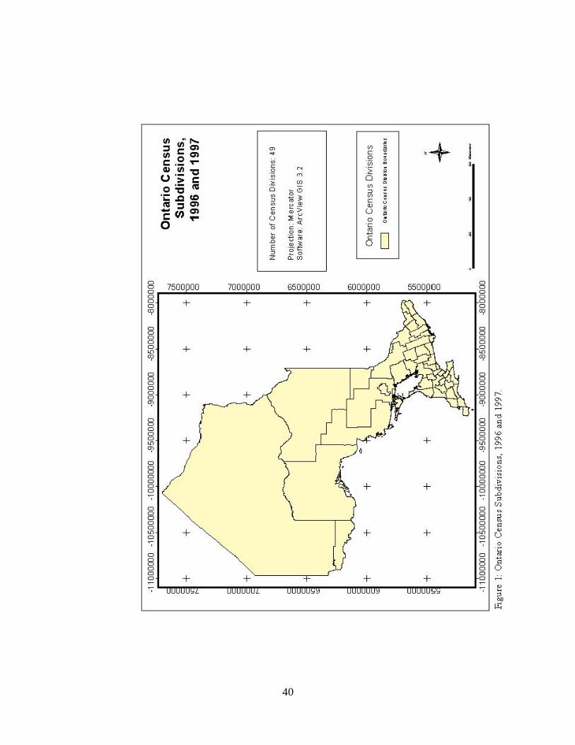
40
41
sex, age, and place of residence of the deceased at the time of death. The variable for the
place of residence is classified in a number of ways, including an aggregation up to the
Statistics Canada geographic reference census division. Census divisions are larger areas
that represent intermediate amalgamations between the municipal and provincial level
(Statistics Canada, 1997). For example, a census subdivision (CSD) might correspond to
the boundaries of a large town, settlement, or First Nations reserve, and a census division
would encompass several census subdivisions, possibly matching up with the borders of a
county or regional municipality. The data for the following investigation are taken from
the mortality database for all deaths for the years of 1996 and 1997.
The digital geographic data that will be used for this investigation were obtained
from the Central East Health Information Partnership, through the Simcoe County
District Health Unit. Basemaps for the aggregation levels of census subdivision and
census division as they existed during the study years were provided in MapInfo table
(.tab) format, which were then converted to ArcView shapefile (.shp) format. This file
conversion was performed with the ‘Universal Translator’ tool in MapInfo Professional
6.5. This function allows the user to import or export MapInfo format data easily by
indicate the location and type of input map file; and then select the type and destination
of the desired output file. Exporting the map files from MapInfo format (.tab) into
shapfile (.shp) format then provided for analysis with subsequent software programs that
interface with ArcView.
42
Additional population estimate data for the CSD’s and CD’s were also obtained
from the Central East Health Information Partnership through the Simcoe County District
Health Unit. Population estimates provide an approximation of the age and gender
characteristics for past inter-censal years using existing data collected from various
sources (Central East Health Information Partnership, 2001). The original source of these
estimates was Statistics Canada, Demography division, which created them under
contract for the both the Ontario Ministry of Finance and Ontario Ministry of Health to
use for planning purposes.
3.4 Methodology
The standardized mortality ratios are calculated for each of the census divisions in
Ontario for both study years (1996, 1997) using the summarized HELPS mortality data
along with the population projections. The formula to calculate a standardized mortality
ratio is fairly straightforward:
SMR = Observed Deaths (in local area) / Expected Deaths (for local area) (1)
Where the number of expected deaths for the local area can be further defined as:
Expected Deaths = {[(Total number of deaths for age group / number of deaths in local
area for age group) * 1000] * local population for age group} / 1000 (2)
43
The raw data were provided from the HELPS system in a SPSS file, containing a
single case record for each death, therefore it was necessary to summarize the cases by
area before calculating the standardized mortality ratios. In addition, this summary was
also required according to the conditions of the research agreement, which states that data
must be aggregated to the minimum geographic unit of census subdivision to prevent
residual disclosure and the identification of individuals (Appendix 1). Calculation of
SMR’s for the census divisions was then performed using a spreadsheet template
developed in Microsoft Excel (Zabowski, 1999). With the template, one could simply
enter the appropriate counts for population (obtained from the census division population
estimate data) and deaths per age group for each of the conditions; and an intermediate
value for the number of expected deaths per CD could be determined (see Equation 2,
previous). The SMR values were automatically computed by dividing the total of
observed deaths by the calculated value for expected deaths (see Equation 1, previous).
Since the process of calculating the SMR values was to be repeated six times (for the
three conditions for both sample years) and for forty-nine census divisions, the template
greatly accelerated this process and is preferred as an alternative to hand calculation.
The use of the aggregation level of census division rather than census
subdivision requires clarification. While the geographic reference variables in the
HELPS Mortality data include references as specific as the census subdivision, this study
used larger census divisions for the analysis and display of the total deaths and
standardized mortality ratio values. Development of a complete understanding of why
this investigation did not take full advantage of the level of geographic precision at which
44
the data were reported requires a review of some of the limitations placed on the data set.
Since restrictions on the HELPS Mortality data state that “cell counts of less than
five…will be treated as confidential…[and be] removed and treated as no data”
(Association of Public Health Epidemiologists in Ontario, 1999), the health researcher
will want to avoid creating tables or maps that display small numbers. For example, if a
great number of census subdivision areas were displayed as ‘No Data’, then such a map
would be less effective in communicating valuable information to the reader. Thus, the
move to a less specific unit of area such as census division may be justified. Another
option that might help to reduce the possibility of small numbers could be to aggregate
mortality data over a number of years. For example, one might add together the number
of deaths due to a specific condition in each census subdivision for a five-year period.
Health researchers may have to try several of these options before finding the most
appropriate method for analysis, finding a balance between the use of precise data and the
avoidance of small number problems.
In order to then analyze the spatial distribution of the SMR values – that is, to
examine for clustering of similar SMR values – two different methods using several
software packages were used. The first of these methods was a combination of two
utilities – the advanced statistical software is S-Plus 2000 (Kaluzny et al., 1998), and
most particularly, the ‘Spatial Stats for ArcView GIS’ module of this program. This
module is an interface that allows the statistical package to be operated within the
ArcView environment, so that the user is able to calculate advanced statistics on any
attribute data for a theme or shapefile that is active in a current session of ArcView.

45
Therefore, since the SMR values for the subdivisions were stored in the Excel
template, it was necessary to import these data files into ArcView. This was
accomplished by saving each calculated SMR value in a separate spreadsheet, and then
storing this as a dBase (IV) database table, which could be opened directly in ArcView.
In order to assign the appropriate index values to the appropriate area location, the.dBase
table was then appended to the attribute table for the census division shapefile, using the
‘join’ feature in ArcView.
The S-Plus Spatial Stats application for ArcView GIS allows the user to calculate
two spatial autocorrelation coefficients – both Moran’s I and Geary’s C statistics, along
with the corresponding p-values to describe their significance. By the p-value method,
one is able to determine the significance of the Moran’s I or Geary’s C spatial
autocorrelation coefficients by comparing the calculated p-value to a specified standard –
most often, a confidence level of 0.05 is used, therefore, the p-value must be less than or
equal to 0.05 for the spatial autocorrelation to be regarded as significant (Lee and Wong,
2001). However, before the coefficients and measures of significance can be calculated,
an intermediate step first needs to be performed. A proximity matrix must be calculated,
as the calculated value for I or C is dependent upon a ‘weighting’ scheme that defines the
spatial relationships between the areas. The weights used to calculate the spatial
autocorrelation statistics can be based upon simple adjacency of area units, proportions of
common boundaries, or the distance between the centroids of areas (Albert et al., 2000).
The weighting scheme selected for this method is the adjusted first-order neighbour

46
weights scheme. Since the census divisions are irregularly shaped polygons, it is possible
that a polygon ‘j’ might be located very close to a specific polygon ‘i’ without sharing a
common border. The adjusted first-order neighbour weights method makes adjustments
to the neighbour weights based on the spatial distances between neighbours (MathSoft,
1998). This modification is accomplished by determining the average distance between
the polygon ‘i’ and all its first-order neighbours, and then admitting all other polygons
that are not directly adjacent to ‘i’ but are enclosed within the average distance into the
neighbourhood structure.
A second method available to calculate the spatial autocorrelation coefficients
made use of only a single GIS software package, ArcView GIS 3.2. ArcView is fairly
adaptable in that it can be ‘customized’ through use of a various programming languages,
including one language specific to ArcView, called Avenue. Avenue and other program
scripts can be written to direct the program to do any number of functions, including
generating additional tables and information, and calculating statistics. For this second
approach, a customized session of ArcView was run using a number of ArcView scripts
that allow for the analysis of spatial patterns. These scripts were obtained from a
statistical resource specially directed toward applications of ArcView GIS (Lee and
Wong, 2001).
The scripts running in the customized ArcView session also allowed for the
calculation of both Moran’s I and Geary’s C, just as was previously determined using the
S-Plus method, but rather than calculating p-values, the scripts instead give an alternate

47
measure of significance – the z-score. In order for Moran’s I autocorrelation coefficient
to be accepted as significant, the z-score must be greater than +1.96 for positive values of
I, or less than –1.96 for negative values of I. For the Geary’s C coefficient to be
significant, the z-score must be greater than +/- 1.96, with any positive z-scores greater
than +1.96 denoting significant negative spatial autocorrelation and any negative z-scores
less than –1.96 denoting significant negative spatial autocorrelation (Lee and Wong,
2001). For the second course of analysis, a row-standardized weights matrix is used.
This weighting scheme scales the weights, or covariance, based upon the number of
neighbours for each region (Kaluzny et al., 1998). Row-standardization functions such
that that the value of any area would receive a fractional influence from the values of
surrounding areas (Lee and Wong, 2001). For example, for a region with five
neighbours, each neighbour pair would have a weight of 0.2.
The choice to use a second, different means of defining the neighbour weights is
grounded in the knowledge that the determination of weights between neighbours is a
crucial part of the analysis of spatial autocorrelation (Griffith, 1995). Neighbour weights
specified by alternate schemes may result in different results in the value and significance
of spatial autocorrelation coefficients. Therefore, by making use of several contrasting
methods of assigning neighbour weights as suggested by several resources (Griffith,
1995; Kaluzny, 1998); it is more likely that evidence indicating significant spatial
autocorrelation in a data set will not be overlooked.
48
In addition, it is important to note that for both methods, these values for I and C
are generated under the free sampling assumption. Free sampling, also know as
normality sampling, assumes that the attribute values for the various areas are
independently drawn from a normal distribution, or in other words, these values are
derived from repeated sampling of a set of values from the normal distribution (Lee and
Wong, 2001). In contrast, non-free or randomization sampling does not assume that the
values are from any specific distribution. The choice between the free/normality
sampling assumption and a counterpart, non-free sampling, can affect the significance of
the spatial autocorrelation coefficient. One may obtain different results by calculating
Moran’s I and Geary’s C on a single data set by following each assumption.
To ensure that the free or normality sampling assumption is reasonable, we can
examine the data for evidence of non-normality (Kaluzny, 1998). Examination of the
skewness and kurtosis statistics for the six distributions of standardized mortality ratio
values will provide evidence as to the fit of the data with reference to the normal
distribution (McGrew and Monroe, 1993). These statistics are listed following in Table
1. The majority of the values for skewness for each of the six distributions are fairly
close to zero, thus implying a symmetrical distribution. The statistics for kurtosis are not
quite as fitting to the normal distribution as could be, however, they still remain fairly
close to the zero mark and do not appear to represent an extremely platykurtic (‘flat’) or
leptokurtic (‘peaked’) distribution (McGrew and Monroe, 1993). In light of these
considerations, there does not appear to be a significantly large deviation from the normal
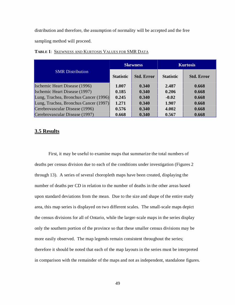
49
distribution and therefore, the assumption of normality will be accepted and the free
sampling method will proceed.
TABLE 1: SKEWNESS AND KURTOSIS VALUES FOR SMR DATA
SMR Distribution
Skewness Kurtosis
Statistic Std. Error Statistic Std. Error
Ischemic Heart Disease (1996) 1.007 0.340 2.487 0.668
Ischemic Heart Disease (1997) 0.185 0.340 0.206 0.668
Lung, Trachea, Bronchus Cancer (1996) 0.245 0.340 -0.02 0.668
Lung, Trachea, Bronchus Cancer (1997) 1.271 0.340 1.907 0.668
Cerebrovascular Disease (1996) 0.576 0.340 4.002 0.668
Cerebrovascular Disease (1997) 0.668 0.340 0.567 0.668
3.5 Results
First, it may be useful to examine maps that summarize the total numbers of
deaths per census division due to each of the conditions under investigation (Figures 2
through 13). A series of several choropleth maps have been created, displaying the
number of deaths per CD in relation to the number of deaths in the other areas based
upon standard deviations from the mean. Due to the size and shape of the entire study
area, this map series is displayed on two different scales. The small-scale maps depict
the census divisions for all of Ontario, while the larger-scale maps in the series display
only the southern portion of the province so that these smaller census divisions may be
more easily observed. The map legends remain consistent throughout the series;
therefore it should be noted that each of the map layouts in the series must be interpreted
in comparison with the remainder of the maps and not as independent, standalone figures.
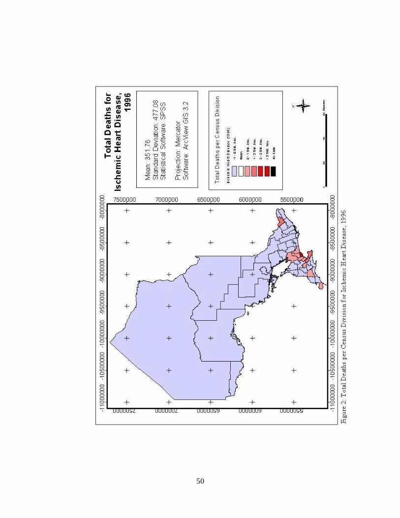
50

51
Figure 3 unavailable
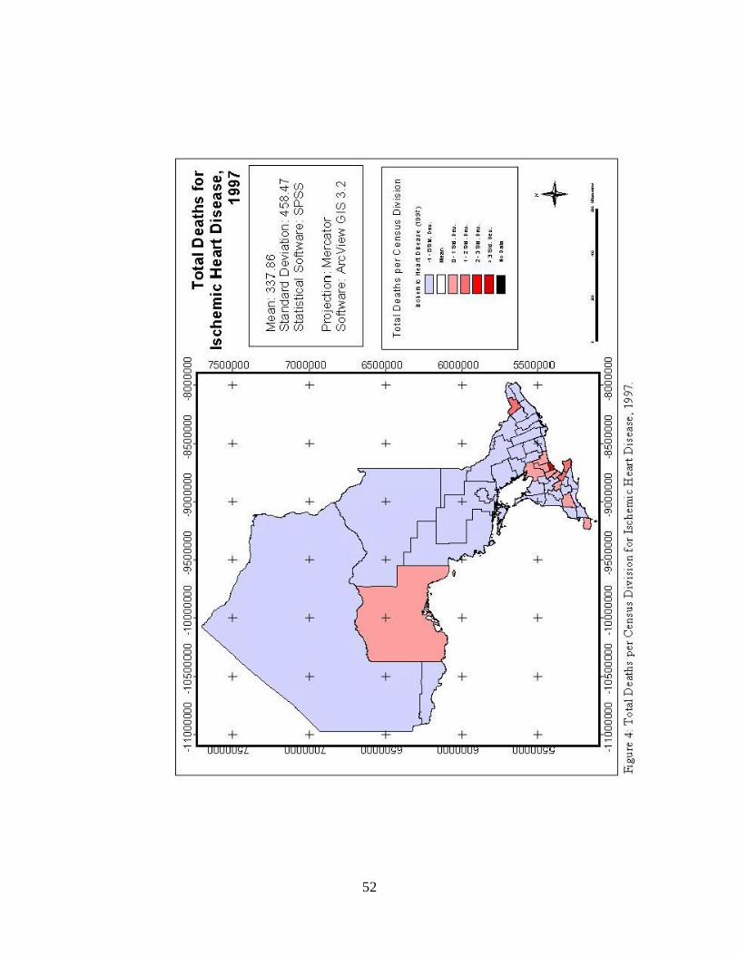
52

53
Figure 5 unavailable
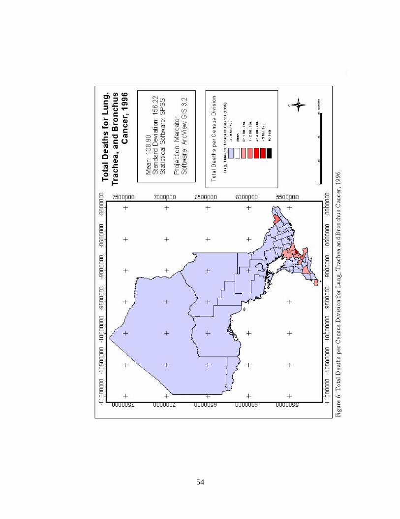
54

55
Figure 7 unavailable
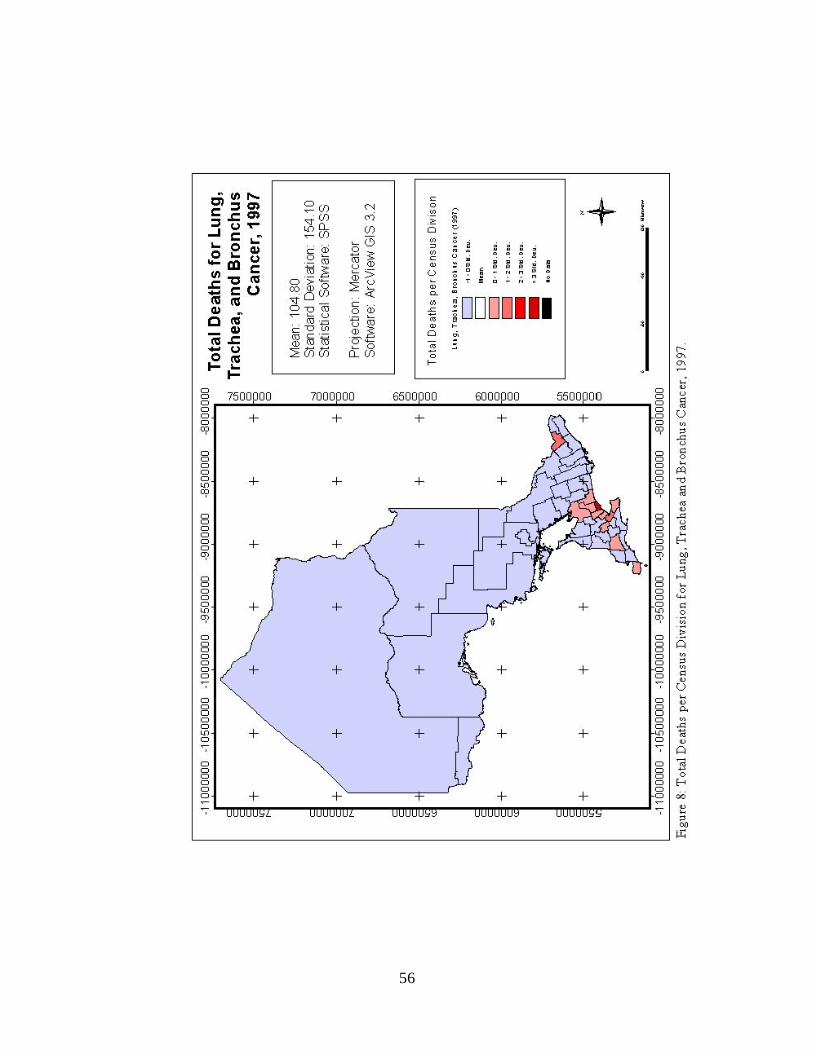
56

57
Figure 9 unavailable
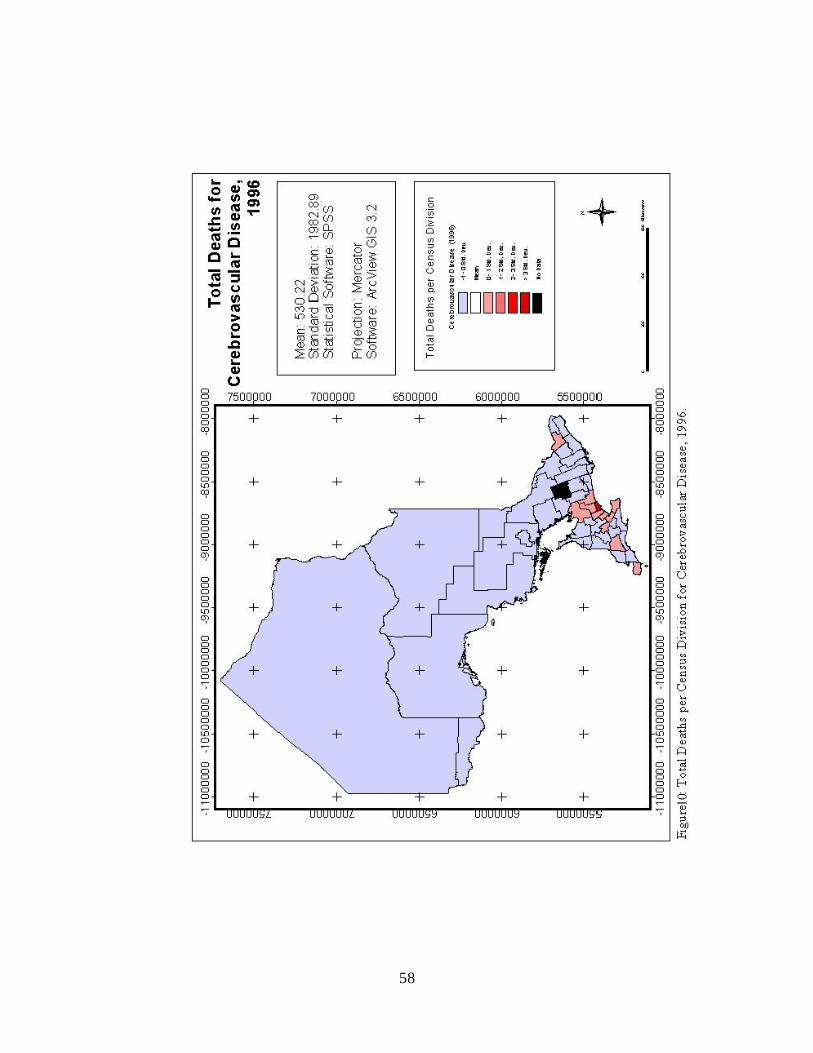
58

59
Figure 11 unavailable
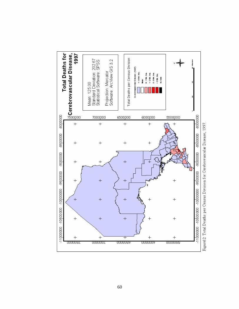
60

61
Figure 13 unavailable
62
A dichromatic colour scheme represents areas where the total number of deaths is within
one standard deviation from the mean (as lightly shaded), with colour intensity increasing
as values increase to within two or three standard deviations. Further, standard
deviations below the mean (negative) are represented in blue shades, and deviations
above the mean (positive) are denoted with deepening shades of pink, red and maroon.
For cases where the total number of deaths in the census division for that study year was
five or less, the true total was suppressed and these cases appear in black, denoted with
‘No Data’.
The most prominent aspect that these maps reveal is the concentration of large
proportions of deaths in areas of greater population. Since the population of the province
is very unevenly distributed with the majority of inhabitants residing in the southern
census divisions, it follows that there would therefore be larger numbers of deaths in
these areas. Accordingly, the maps indicate a clustered spatial pattern, where areal units
possessing values that are, for example, three standard deviations above the mean are
located nearby to other areal units with similar values.
The features of these choropleth maps clearly demonstrate the need for care and
attention when performing mapping of mortality and other health-related data (Goodman
and Wenneberg, 1999). An understanding of the nature of the data being mapped is
absolutely essential – without the knowledge of the general population distribution of
Ontario, incorrect or misrepresentative inferences could have been interpreted from the
figures. In addition, the experience also demonstrates the limitations of mapping crude
63
values that have not been adjusted to account for population variations in study area
geographic units or differences in the age structures within these areas. It has been shown
that the comparison of such basic numbers can be problematic due to differences in the
‘environmental’ characteristics of an area. The use of a standardized index like the
standardized mortality ratio (SMR) is therefore necessary for the purposes of mapping
and other analytic work when the data under investigation deal with phenomenon (i.e.
disease mortality) that are affected by factors such as the age structure of the population
in the area. This assertion now leads to the next products created in the investigation –
the plotting and geostatistical analysis of the standardized mortality ratios for the Ontario
census divisions.
The standardized mortality ratio values for each of the census divisions are
displayed graphically in another series of associated diagrams (Figures 14 through 25).
The areas of greatest interest to epidemiologists and public health officials in this series
of maps would be census divisions where the value of the SMR is substantially higher
than one (1), since this indicates areas where the number of observed deaths is greater
than the number of deaths expected according to the provincial trends for that year. The
1996 and 1997 SMR values of the selected conditions for the census divisions are
displayed by a ‘user-defined’ classification scheme, again using a dichromatic colour
scheme. Census divisions with standardized mortality ratios from 0 to 0.5 are displayed
in dark blue and 0.501 to 0.9 in light blue; while SMR values that are from 0.901 to 1.10
are shown as transparent. Census divisions where the SMR value is between 1.101 and
1.50 are shown in light red, and finally, areas where the SMR exceeds 1.5 are indicated
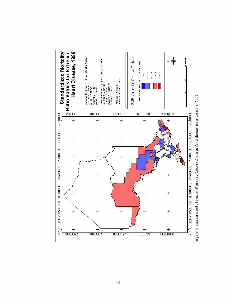
64

65
Figure 15 unavailable
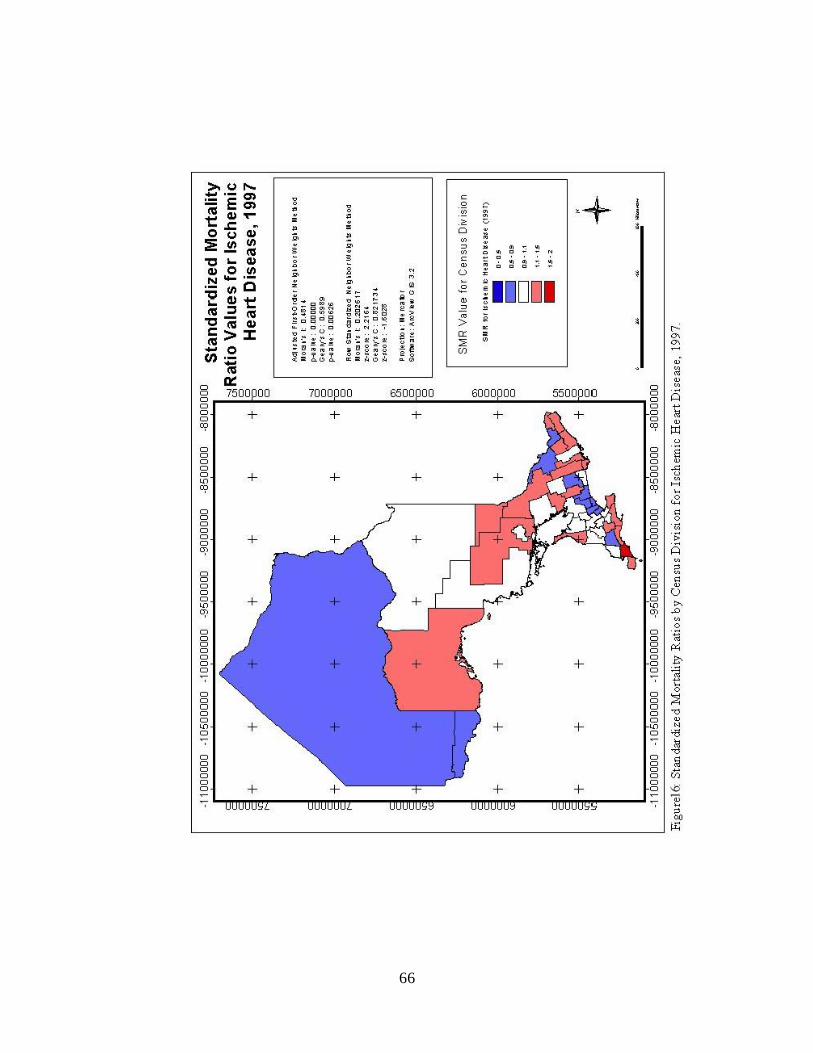
66

67
Figure 17 unavailable
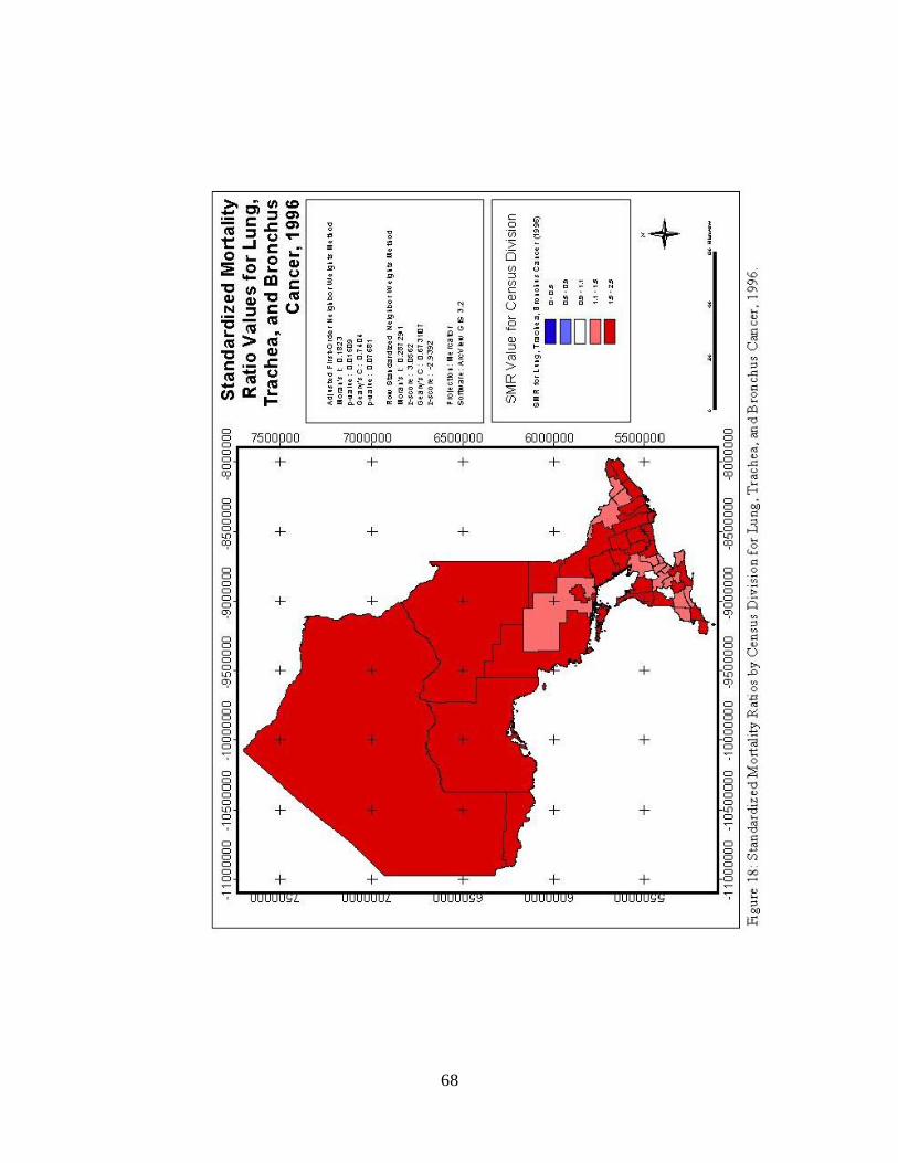
68

69
Figure 19 unavailable
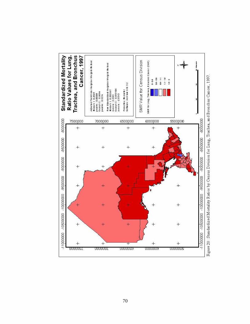
70

71
Figure 21 unavailable
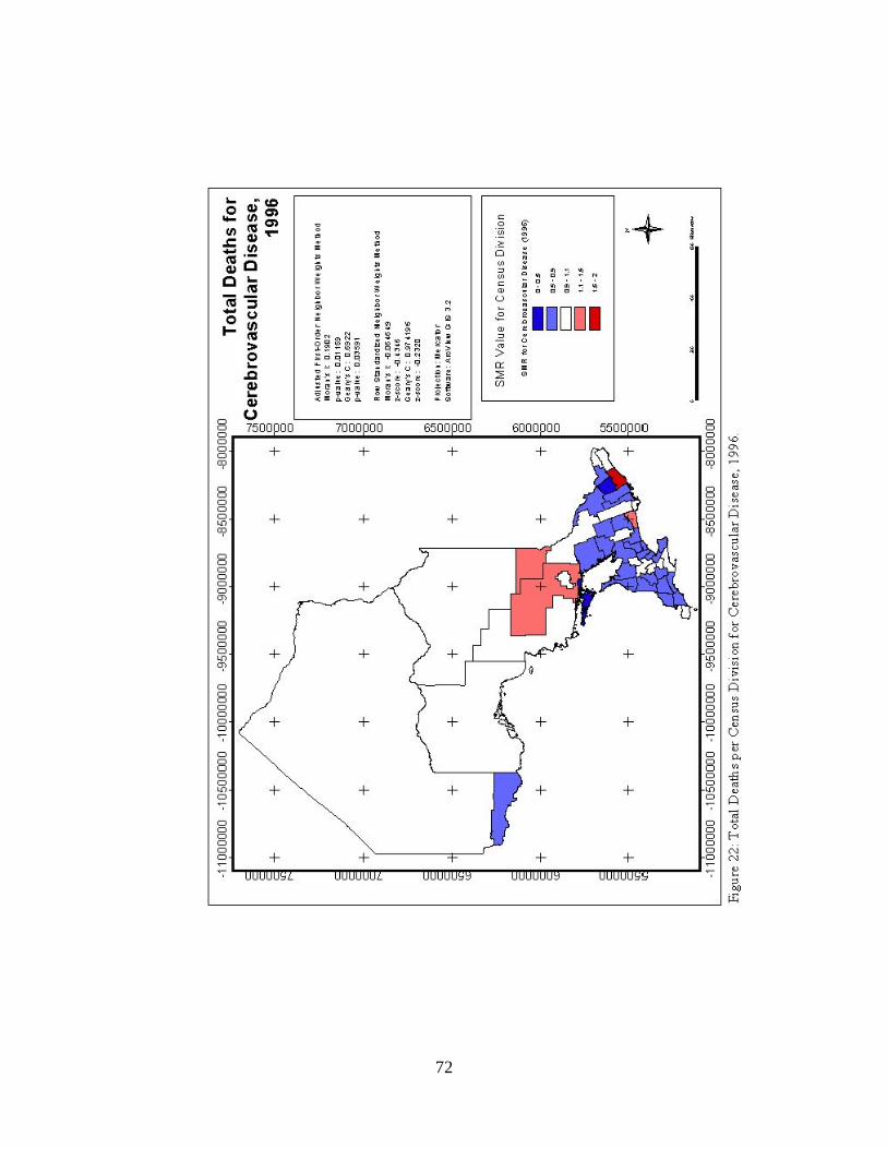
72

73
Figure 23 unavailable
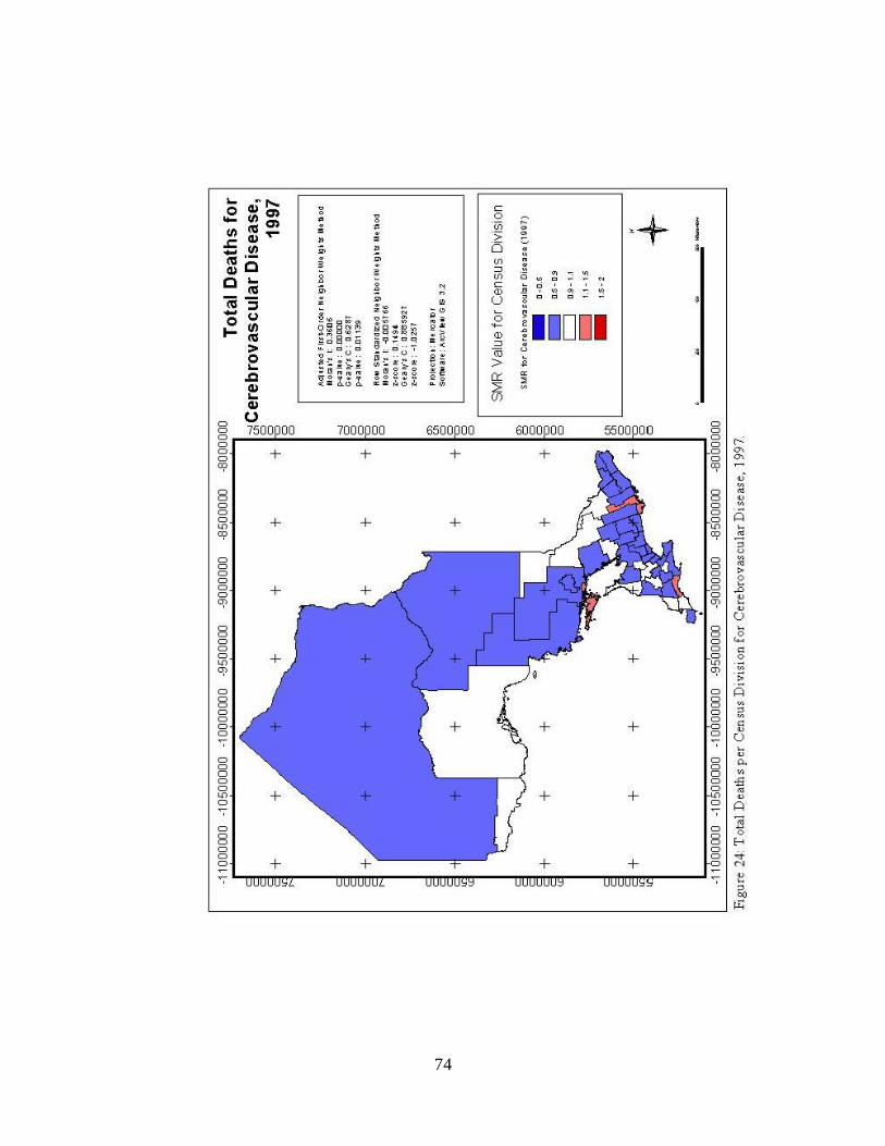
74

75
Figure 25 unavailable
76
in dark red.
Visual inspection of the standardized mortality ratio figures reveals a number of
interesting patterns. The maps of ischemic heart disease SMR values for 1996 and 1997
both show a large number of the census divisions throughout the province that possess a
standardized mortality ratio near one (1). While some SMR values between 0.501 and
0.90, and between 1.10 and 1.50 are present, there are no extremely high or low cases.
Further, it appears that the census divisions with standardized mortality ratios within the
same class may be slightly clustered; however, the map takes on more of a
‘checkerboard’ appearance that is not consistent with positive spatial autocorrelation (Lee
and Wong, 2001).
The images representing the spatial distribution of standardized mortality ratios
for lung, trachea, and bronchus cancer in 1996 and 1997 show very little variation in the
values of SMR by census division. The 1996 image displays the vast majority of census
divisions with SMR values from 1.501 to 2, with very few areas possessing values
between 1.101 and 1.5, and no areas having an SMR of less than 1. The 1997 image
remains relatively the same, with only one census division displaying a standardized
mortality ratio of between 0.501 and 0.90. There appears to be a dramatic amount of
clustering of similar SMR values present in these two diagrams, but this grouping may in
fact be due the small amount of variation in the SMR values themselves. It is recognized
that if taken as standalone map images, these figures would be less effective in
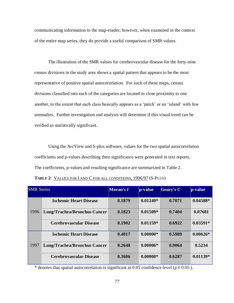
77
communicating information to the map-reader; however, when examined in the context
of the entire map series, they do provide a useful comparison of SMR values.
The illustration of the SMR values for cerebrovascular disease for the forty-nine
census divisions in the study area shows a spatial pattern that appears to be the most
representative of positive spatial autocorrelation. For each of these maps, census
divisions classified into each of the categories are located in close proximity to one
another, to the extent that each class basically appears as a ‘patch’ or an ‘island’ with few
anomalies. Further investigation and analysis will determine if this visual trend can be
verified as statistically significant.
Using the ArcView and S-plus software, values for the two spatial autocorrelation
coefficients and p-values describing their significance were generated in text reports.
The coefficients, p-values and resulting significance are summarized in Table 2.
TABLE 2: VALUES FOR I AND C FOR ALL CONDITIONS, 1996/97 (S-PLUS)
SMR Series Moran's I p-value Geary's C p-value
1996
Ischemic Heart Disease 0.1879 0.01249* 0.7071 0.04588*
Lung/Trachea/Bronchus Cancer 0.1823 0.01509* 0.7404 0.07681
Cerebrovascular Disease 0.1902 0.01159* 0.6922 0.03591*
1997
Ischemic Heart Disease 0.4817 0.00000* 0.5989 0.00626*
Lung/Trachea/Bronchus Cancer 0.2648 0.00006* 0.9064 0.5234
Cerebrovascular Disease 0.3606 0.00000* 0.6287 0.01139*
* denotes that spatial autocorrelation is significant at 0.05 confidence level (p 0.05 ).

78
The S-Plus method of calculating the Moran’s I and Geary’s C spatial
autocorrelation coefficients has provided evidence that significant spatial autocorrelation
exists according to the Moran’s I coefficients for the maps of SMR values for ischemic
heart disease (1996 and 1997); lung, trachea, and bronchus cancer (1996 and 1997); and
cerebrovascular disease (1996 and 1997), under the adjusted first-order neighbour
weighting scheme. Further, the coefficients for Geary’s C under the adjusted first-order
neighbour weighting scheme indicate significant spatial autocorrelation for ischemic
heart disease (1996 and 1997) and cerebrovascular disease (1996 and 1997). The only
cases in which the spatial autocorrelation coefficients were deemed to be not statistically
significant were for lung, trachea, and bronchus cancer (both 1996 and 1997), according
to the Geary’s C statistics only.
While the spatial autocorrelation coefficients for the standardized mortality ratios
of the six distributions were significant (with the exception of the Geary’s C coefficients
for lung, trachea, and bronchus cancer), this does not necessarily signify the strength or
extent of the spatial autocorrelation. In common practice, perfect positive spatial
autocorrelation is indicated by a significant Moran’s I coefficient of +1 (Cliff and Ord,
1981); however, there may be some exceptions to this guideline, dependent on the
weighting of spatial neighbours (Griffith and Amrhein, 1997). The significant I
coefficients for this example varied from 0.1879 to 0.4817, representing fairly strong,
while not perfect, positive spatial autocorrelation. Further, Geary’s C will take on a value
of zero in cases of perfect positive spatial autocorrelation, as opposed to a value of +1 for
a random spatial distribution, or +2 where there is evidence of perfect negative spatial
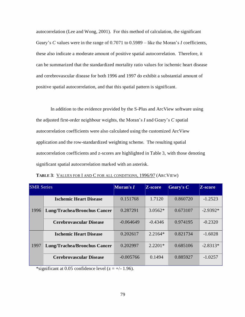
79
autocorrelation (Lee and Wong, 2001). For this method of calculation, the significant
Geary’s C values were in the range of 0.7071 to 0.5989 – like the Moran’s I coefficients,
these also indicate a moderate amount of positive spatial autocorrelation. Therefore, it
can be summarized that the standardized mortality ratio values for ischemic heart disease
and cerebrovascular disease for both 1996 and 1997 do exhibit a substantial amount of
positive spatial autocorrelation, and that this spatial pattern is significant.
In addition to the evidence provided by the S-Plus and ArcView software using
the adjusted first-order neighbour weights, the Moran’s I and Geary’s C spatial
autocorrelation coefficients were also calculated using the customized ArcView
application and the row-standardized weighting scheme. The resulting spatial
autocorrelation coefficients and z-scores are highlighted in Table 3, with those denoting
significant spatial autocorrelation marked with an asterisk.
TABLE 3: VALUES FOR I AND C FOR ALL CONDITIONS, 1996/97 (ARCVIEW)
SMR Series Moran's I Z-score Geary's C Z-score
1996
Ischemic Heart Disease 0.151768 1.7120 0.860720 -1.2523
Lung/Trachea/Bronchus Cancer 0.287291 3.0562* 0.673107 -2.9392*
Cerebrovascular Disease -0.064649 -0.4346 0.974195 -0.2320
1997
Ischemic Heart Disease 0.202617 2.2164* 0.821734 -1.6028
Lung/Trachea/Bronchus Cancer 0.202997 2.2201* 0.685106 -2.8313*
Cerebrovascular Disease -0.005766 0.1494 0.885927 -1.0257
*significant at 0.05 confidence level (z = +/- 1.96).

80
The results for the second method of calculating Moran’s I and Geary’s C also
reveal some evidence of significant spatial autocorrelation according to the row-
standardized weighting scheme. According to the Moran’s I spatial autocorrelation
coefficients and the resulting z-score consistent with the row-standardized weighting
scheme, significant spatial autocorrelation exists for both the 1996 and 1997 SMR values
for lung, trachea, and bronchus cancer. The results for the Geary’s C coefficient and z-
score corroborate the Moran’s I results – with values of 0.673107 and 0.685106, and z-
scores of less than –1.96, they are also indicative of significant spatial autocorrelation. In
addition, the 1997 standardized mortality ratios for ischemic heart disease exhibit
significant autocorrelation according to the I coefficient and z-score, but this result is not
consistent with the Geary’s C coefficient and z-score.
Since the z-score associated with the Moran’s I correlation coefficients for
ischemic heart disease (1996) and cerebrovascular disease (1996 and 1997) under the
row-standardized neighbour weighting scheme are less than the required +/- 1.96, there is
not enough evidence to confirm that the spatial autocorrelation is significant. Although
the I coefficient for ischemic heart disease in 1996 does appear to be significant, the
Geary’s C coefficient and corresponding z-value do not support this finding. Under the
row-standardized weights method, the Geary’s C z-score for ischemic heart disease and
cerebrovascular disease for both study years are all non-significant.
The calculation of the Moran’s I and Geary’s C spatial autocorrelation
coefficients and appropriate measures of significance has provided evidence that

81
significant positive spatial autocorrelation exists for several of the spatial distributions of
standardized mortality ratios in the study area. According to the adjusted first-order
neighbour weighting scheme, autocorrelation coefficients and resultant p-values indicate
that the standardized mortality ratios for ischemic heart disease in 1996 and 1997, and
cerebrovascular disease in 1996 and 1997 exhibit considerable significant positive spatial
autocorrelation. Further, according to the row-standardization neighbour weights
method, the statistics indicate that the SMR values lung, trachea, and bronchus cancer in
1996 and 1997 also display a considerable amount of significant positive spatial
autocorrelation.
Differences were also observed in the values of the spatial autocorrelation
coefficients depending on the weighting scheme that was used to define the spatial
neighbours within the study area. While the actual spatial autocorrelation coefficient
values were often quite similar when calculated according to each weighting scheme; the
status of the resulting p-values and/or z-scores changed the outcome of the test
noticeably. This observation remains in keeping with the earlier statement that alternate
schemes may result in different results in the value and significance of spatial
autocorrelation coefficients (Kaluzny, 1998).
3.6 Conclusion
The hypothesis that mortality rates will exhibit a substantial amount of positive
spatial autocorrelation was investigated using two spatial autocorrelation coefficients –

82
Moran’s I and Geary’s C – as indexes to look for the presence of disease ‘hotspots’ or the
occurrence of spatial clusters where mortality rates exhibit a high degree of similarity. In
order to most effectively analyze the spatial distribution of the standardized mortality
ratio values – that is, to examine for the clustering of similar SMR values – two different
methods using several software packages were used. Both an adjusted first-order
neighbour weighting scheme as well as a row-standardized weighting scheme were used
to determine the significance of the spatial autocorrelation coefficients, and the different
effects of these schemes were observed as variations in the values of I and C and the
corresponding measures of significance.
The standardized mortality ratios for ischemic heart disease, lung cancer
(including cancer of the trachea and bronchus), and cerebrovascular disease were all
found to exhibit a considerable degree of significant positive spatial autocorrelation
(according to at least one of the methods). This occurred when the spatial autocorrelation
coefficients were calculated according to either the adjusted first-order neighbour or row-
standardized weighting schemes. This evidence supports the initial hypothesis that
mortality rates reveal a substantial amount of significant positive spatial autocorrelation.
In conclusion, it does appear that mortality rates for ischemic heart disease, lung
cancer, and cerebrovascular disease do tend to exhibit a specific spatial pattern within
Ontario, based upon the observations and calculations from the 1996 and 1997 Ontario
Ministry of Health and Long Term Care Health Planning Database. Due to the significant
amount of positive spatial autocorrelation, the higher values for the standardized
83
mortality ratios cluster together, as opposed to displaying a dispersed or random spatial
distribution.
3.7 Suggestions for Future Research
The knowledge provided by this research can be utilized by public health officials
to further investigate any processes that could have contributed to the spatial pattern of
mortality within the study area. The insight provided by Moran’s I and Geary’s C spatial
autocorrelation coefficients for the purposes of cluster detection in mortality rates is
merely a beginning for applications of geostatistics and spatial analysis techniques in
public health applications. Once exploratory spatial analysis such as the calculation of
map pattern descriptors has been completed, later work could prove be more associative
and confirmative in approach (Douven and Scholten, 1995). In cases where the spatial
autocorrelation of mortality rates is found to be significant, public health officials may
focus attention on ‘hot spots’ and target further investigations to determine the effects of
other explanatory variables (Walter, 1992b).
Opportunities for further investigation related to this research project could
include the integration of additional data into the health-oriented geographic information
system. In order to take a more associative approach to understanding the spatial patterns
associated with mortality rates, one could incorporate data into the geographic
information system that describes some attribute (i.e. socioeconomic status, level of
urbanization) that is hypothesized to be associated or contributes to high mortality rates

84
(Walter, 1992b). If there is sufficient evidence of association between the variable and
the mortality rates, then one could use this additional data to develop a spatial model. For
example, one might attempt the use of geostatistical techniques to develop a model that
would predict mortality rates or potential risk based upon both the extent of spatial
autocorrelation and the effect of some other contributing variable (Isaaks and Stivastava,
1989).
There are numerous other possibilities for other projects that public health
researchers and/or individuals skilled in the operation of geographic information systems
and methods of spatial analysis may want to collaborate upon. Most recently, the
eastward movement of the West Nile virus – a strain of encephalitis that can be fatal to
segments of the population – in North America has initiated the development of new,
more accurate public health databases detailing the specific locations of West Nile cases
in birds, larger mammals, and humans (Rose, 2001). In the past year, even local public
health organizations such as the Simcoe County District Health Unit in Barrie, Ontario
have developed workable West Nile Virus databases (Guarda, Personal Communication,
July 16, 2001). The availability of well-designed, geographically precise health attribute
databases presents new options for those interested in using GIS and spatial analysis.
Related projects may lead to discoveries that would benefit the fields of both geography
and public health.
85
References
Note: All URL’s current as of August 2001.
Albert, D.P., W.M. Gesler, and B. Levergood. 2000. Spatial Analysis, GIS, and Remote
sensing applications in the health sciences. Chelsea, Michigan: Ann Arbor Press.
Aronoff, S. 1995. GIS: A mangement perspective. Ottawa, ON: WDL Publications.
Association of Public Health Epidemiologists in Ontario (APHEO). 1999. Core
Population Health Indicators for Ontario – Mortality. [WWW document]
http://www.cehip.org/apheo/Committees/prov4ab.htm
Bakkes, J.A. 1995. Meta-information systems for environment and health. De Lepper,
M.J.C., H.J. Scholten, and R.M. Stern (Eds.). 1995. The added value of
geographical information systems in public and environmental health. Norwell,
MA: Kluwer Academic Publishers. pp. 41-50.
Bailey, T.C. and A.C. Gatrell. 1995. Interactive Spatial Data Analysis. Essex, UK:
Longman Group Ltd.
Braga, M., C. Cislaghi, G. Luppi, and C. Tasco. 1998. A multipurpose, interactive
mortality atlas of Italy. Gatrell, A.C. and M. Loytonen (Eds.). 1998. GIS and
Health. Philadelphia, PA: Taylor and Francis, Ltd. pp. 125-138.
Bretas, G. 1994. Geographical information systems for the study and control of malaria.
De Savigny, D. and P. Wijeyarantne (Eds.). 1995. GIS for health and the
environment: Proceedings of an international workship held in Colombo, Sri
Lanka 5-10 September 1994. Ottawa, ON: International Development Research
Centre. pp. 89-97.
Brown, P., A. Hirschfield, and J. Marsden. 1995. Analysising spatial patterns of disease:
some issues in the mapping of incidence data for relatively rare conditions. De
Lepper, M.J.C., H.J. Scholten, and R.M. Stern (Eds.). 1995. The added value of
geographical information systems in public and environmental health. Norwell,
MA: Kluwer Academic Publishers. pp. 145-163.
Burrough, P.A. and R.A. McDonnell. 1998. Principles of Geographical Information
Systems. New York, NY: Oxford University Press.
Central East Health Information Partnership. 2001. Population data cubes update: User’s
guide. Newmarket, ON: Central East Health Information Partnership.
86
Clark, K.C., S.L. McLafferty, and B.J. Templaski. 1996. On epidemiology and GIS: A
review and discussion of future directions. Emerging Infectious Diseases 2(2),
85-92.
Cliff, A.D. and J.K. Ord. 1981. Spatial processes: Models and applications. London,
UK: Pion, Ltd.
Cole, L. 2001. Personal Communication. Project Manager. Geomatics Division, City
of Ottawa. Ottawa, Ontario.
County of Simcoe. 2000. Executive Summary of LINC and Simcoe County GIS section.
[WWW document] http://www.county.simcoe.on.ca/services/gis/gis2.shtml
Douven, W. and H.J. Scholten. 1995. Spatial analysis in health research. De Lepper,
M.J.C., H.J. Scholten, and R.M. Stern (Eds.). 1995. The added value of
geographical information systems in public and environmental health. Norwell,
MA: Kluwer Academic Publishers. pp. 117-133.
Elliot, P. J.C. Wakefield, N.G. Best, and D.J. Briggs. 2000. Spatial epidemiology:
Methods and applications. New York, NY: Oxford University Press.
Environmental Systems Research Institute, Inc (ESRI). 2001. ESRI Canada Corporate
Website. [WWW document] http://www.esricanada.com
Environmental Systems Research Institute, Inc (ESRI). 1996. ArcView GIS: The GIS
for everyone. Redlands, CA: Environtmental Systems Research Institute, Inc.
Gatrell, A.C. and C.E. Dunn. 1995. Geographical information systems and spatial
epidemiology: Modelling the possible association between cancer of the larynx
and incineration in north-west England. De Lepper, M.J.C., H.J. Scholten, and
R.M. Stern (Eds.). 1995. The added value of geographical information systems
in public and environmental health. Norwell, MA: Kluwer Academic Publishers.
pp. 215-235.
Gilbert, C. 1999. Are we there yet? GeoAsiaPacific. April 1999.
Goodman, D.C. and J.E. Wennberg. 1999. Maps and health: The challenges of
interpretation. Journal of Public Health Management and Practice 5(4). pp. xii-
xvi.
Gregario, D.I., E. Cromley, R. Mrozinski, and S.J. Walsh. 1999. Subject loss in spatial
analysis of breast cancer. Health and Place 5. pp. 173-77.
Griffith, D.A. 1995. Some guidelines for specifying the geographic weights matrix
contained in spatil statistical models. Arlinghaus, S.L. (Ed.) Practical Handbook
of Spatial Statistics. Boca Raton, FL: CRC Press, Inc. pp. 65-82.
87
Griffith, D.A. and C.G. Amrhein. 1997. Multivariate statistical analysis for geographers.
Upper Saddle River, NJ: Prentice Hall, Inc.
Guarda, B. 2001. Personal Communication. Epidemiologist. Simcoe County District
Public Health Unit. Barrie, Ontario.
Heath, D.W. 1995. Organizational aspects of geographical information systems. De
Lepper, M.J.C., H.J. Scholten, and R.M. Stern (Eds.). 1995. The added value of
geographical information systems in public and environmental health. Norwell,
MA: Kluwer Academic Publishers. pp. 87-97.
Hughes, J.R. 2000. GPS crosses the chasm. GeoWorld. January 2000.
Information and Privacy Commissioner of Ontario. 1998. A Mini-Guide to Ontario’s
Municipal Freedom of Information and Protection of Privacy Act. Information
and Privacy Comission of Ontario.
http://www.ipc.on.ca/english/acts/pocket/mini-m.htm
Isaaks, E.H. and R.M. Srivastava. 1989. Applied geostatistics. New York, NY: Oxford
University Press.
Kaluzny, S.P., S.C. Vega, T.P. Cardoso, and A.A. Shelley. 1998. S+ Spatial Stats.
Seattle, WA: MathSoft, Inc.
Kelsey, J.L., W.D. Thompson, and A.S. Evans. 1986. Methods in Observational
Epidemiology. New York, NY: Oxford University Press.
Kulldorff, M. 1999. GIS (GIS) and community health: Some statistical issues. Journal
of Public Health Management and Practice 5(4), 100-106.
Lang, L. 2000. GIS for Health Organizations. Redlands, CA: Environmental Systems
Research Institute, Inc.
Lee, C.V. and J.L. Irving. 1999. Sources of spatial data for community health planning.
Journal of Public Health Management Practice 5(4). pp. 7-22.
Lee, J. and D.W.S. Wong. 2001. Statistical Analysis with ArcView GIS. Toronto:
Wiley and Sons.
Lilienfeld, A.M. and D.E. Lielienfeld. 1980. Foundations of Epidemiology, 2nd Ed.
New York, NY: Oxford University Press.
Loslier, L. 1994. Geographical information science (GIS) from a health perspective. De
Savigny, D. and P. Wijeyarantne (Eds.). 1995. GIS for health and the
environment: Proceedings of an international workship held in Colombo, Sri
88
Lanka 5-10 September 1994. Ottawa, ON: International Development Research
Centre. pp. 13-20.
Maes, J. and M.H. Cornaert. 1995. Data aspects of geographical information systems.
De Lepper, M.J.C., H.J. Scholten, and R.M. Stern (Eds.). 1995. The added value
of geographical information systems in public and environmental health.
Norwell, MA: Kluwer Academic Publishers. pp. 99-114.
Manson, P. 2000. GPS-based tools for GIS data maintenance. GeoWorld. February
2000.
MapInfo Corporation. 2001. MapInfo Professional 6.5. Troy, NY: MapInfo
Corporation.
MathSoft, Inc., Data Analysis Products Division. 1998. S-Plus Stats for ArcView Help.
Seattle, WA: MathSoft.
McElroy, J.A., L.D. Andersen, A.Trenthan-Dietz, R.S. Kirby, M.K. Clayton and P.L.
Remington. 2001. Assigning atrazine exposure levels in a case-control study
using spatial analysis of well water testing data. American Journal of
Epidemiology 153(11). pp. 452.
McGrew, J.C., and C.B. Monroe. 1993. Statistical problem solving in geography. New
York, NY: McGraw-Hill .
Meade, M.S., and F.J. Earickson. Medical geography, 2nd Ed. New York, NY: Guilford
Press.
Melnick, A.L. and D.W. Fleming. 1999. Modern GIS: Promises and Pitfalls. Journal of
Public Health Management and Practice 5(2), 8-10.
Monmonier, M. 1996. How to lie with maps. Chicago, Ill.: University of Chicago Press.
Montain, J.M. 2001a. Integrating GIS into public health applications. Newmarket, ON:
Central East Health Information Partnership. Available online at:
http://www.cehip.org.
Montain, J.M. 2001b. Summary Report: GIS at Simcoe County District Health Unit.
Barrie, ON: Simcoe County District Health Unit.
Nobre, F.F. and M. Sa Carvalho. Spatial and temporal analysis of epidemiological data.
De Savigny, D. and P. Wijeyarantne (Eds.). 1995. GIS for health and the
environment: Proceedings of an international workship held in Colombo, Sri
Lanka 5-10 September 1994. Ottawa, ON: International Development Research
Centre. pp. 21-31.
89
Pan American Health Organization. 2000. GIS in health, basic concepts. Washington,
D.C.: OPS.
Potter, J. 2001. Personal Communication. Health Information Analyst. City of Ottawa
Health Department. Ottawa, Ontario.
Reader, S. 1994. The present state of GIS and future trends. De Savigny, D. and P.
Wijeyarantne (Eds.). 1995. GIS for health and the environment: Proceedings of
an international workship held in Colombo, Sri Lanka 5-10 September 1994.
Ottawa, ON: International Development Research Centre. pp. 3-12.
Roberts, N. 2001. Personal Communication. Manager. Client Services (GIS), Regional
Municipality of Waterloo. Waterloo, Ontario.
Roper, W.L. and G.P. Mays. 1999. GIS and public health policy: A new frontier for
improving community health. Journal of Public Health Management and Practice
5(2), 6-7.
Rose, R.L. 2001. Pesticides and public health: Integrated methods of mosquito
management. Emerging Infectious Diseases 7(1), 17-23.
Rushton, G., G. Elmes, and R. McMaster. 2000. Considerations for improving GIS
research in public health. URISA Journal 12(2), 31-49.
Scholten, H.J. and M.J.C. De Lepper. 1995. An introduction to geographical
information systems. De Lepper, M.J.C., H.J. Scholten, and R.M. Stern (Eds.).
1995. The added value of geographical information systems in public and
environmental health. Norwell, MA: Kluwer Academic Publishers. pp. 53-70.
Siffel, C., A. Correa, and L.Y.C. Wong. 2001. Developing methods for temporal-spatial
analysis of birth defects. American Journal of Epidemiology 153(11). pp. 580.
Statistics Canada. 1997. 1997 Geography Catalogue. Ottawa, ON: Minister of
Industry.
Thomas, R.W. 1990. Issues in spatial epidemiology. Spatial Epidemiology. London,
UK: Pion Ltd.
Twigg, L. 1990. Health based geographical information systems: Their potential
examined in light of existing data sources. Social Science Medicine 30(1), 143-
55.
Van Beurden, A.U.C.J. and M.J.C. De Lepper. 1995. The integration of information in
geographical information systems. De Lepper, M.J.C., H.J. Scholten, and R.M.
Stern (Eds.). 1995. The added value of geographical information systems in
90
public and environmental health. Norwell, MA: Kluwer Academic Publishers.
pp. 71-86.
Vins, W., K. Vaughn, and M. Stefanak. 2001. GIS and environmental health: Locating
wells for a groundwater monitoring program in Mahoning County. Public Health
GIS News and Information 38. January 2001. Office of Research and
Methodology, National Center for Health Statistics. pp. 10-14.
Walden, T. 2001. Personal Communication. GIS Programmer/Analyst. Regional
Municipality of Waterloo. Waterloo, Ontario.
Walter, S.D. 1993. Assessing spatial patterns in disease rates. Statistics in Medicine
12(19/20). pp. 1885-1894.
Walter, S.D. 1992a. The analysis of regional patterns in health data. I. Distributional
Considerations. American Journal of Epidemiology 136(6). pp. 730-741.
Walter, S.D. 1992b. The analysis of regional patterns in health data. II. The power to
detect environmental effects. American Journal of Epidemiology, 136(6). pp.
742-759.
Wartenberg, D. and M. Greenberg. 1990. Space-time models for the detection of
clusters of disease. R.W. Thomas (Ed.). Spatial Epidemiology. London, UK:
Pion Ltd.
Westlake, A. 1995. Strategies for the use of geography in epidemiological analysis. De
Lepper, M.J.C., H.J. Scholten, and R.M. Stern (Eds.). 1995. The added value of
geographical information systems in public and environmental health. Norwell,
MA: Kluwer Academic Publishers. pp. 135-144.
Wojdyla, D., L. Poletto, C. Cuesta, C. Badler, and M.E. Passamonti. 1996. Cluster
analysis with constraints: Its use with breast cancer mortality rates in Argentina.
Statistics in Medicine 15(7/9). pp. 741-746.
Xie, L., R. Semenciw, and A.M Ugnat. 2001. Geographic clusters of breast, colorectal,
lung and prostate cancer incidence in Canada. American Journal of Epidemiology
153(11). pp. 350.
Yasnoff, W.A. and E.J. Sondik. 1999. Geographic information systems (GIS) in public
health in the new millennium. Journal of Public Health Management and Practice
5(4). pp. vii-xi.
Zabowski, G. 1999. Using Excel for statistics and data analysis. Don Mills, ON:
Addison Wesley Longman, Ltd.

91
Appendix 1: Research Agreement
The Research Agreement for access to the data used in this project reads:
1. Datafiles will be maintained in a secure location on the Simcoe County District
Health Unit network and will not be removed from the agency.
2. Access to the datafiles will be for the purpose of investigating the public health
application of geographic information systems as outlined in the thesis proposal.
3. In order to prevent the residual disclosure of any individual, cell counts less than
five in the tables will be treated as confidential. Data will be aggregated to the
larger, less specific census area unit of Census Subdivision to reduce the potential
for having cell counts of less than five. Any cell counts of less than five that
occur after aggregation will be removed and treated as no data.
4. The Simcoe County District Health Unit is to be notified a breach in any of the
conditions set out in this agreement.
5. The following acknowledgement shall be used for the source of the data. (Name
of datafile, Ontario Ministry of Heath and Long Term Care, Year)