Integrating Dock-Door Assignment and Vehicle Routing in Cross-Docking

Furkan Enderer

A Thesis

in the Department

of

Mechanical and Industrial Engineering

Presented in Partial Fulfilment of the Requirements

for the Degree of Master of Applied Science (Industrial Engineering) at

Concordia University

Montreal, Quebec, Canada

April 2014

c©Furkan Enderer, 2014

CONCORDIA UNIVERSITY

School of Graduate Studies

This is to certify that the thesis is prepared

By: Furkan Enderer

Entitled: Integrating Dock-Door Assignment and Vehicle Routing in Cross-Docking

and submitted in partial fulfillment of the requirements for the degree of

Master of Applied Science (Industrial Engineering)

Complies with the regulations of the University and meets the accepted standards with respect to originality and quality.

Signed by the final examining committee:

________________________ Chair

________________________ Examiner

________________________ Examiner

________________________ Supervisor

________________________ Supervisor

Approved by ________________________________________

Chair of Department or Graduate Program Director

___________2014 ________________________________________

Dean of Faculty of Arts and Science

Abstract

Integrating Dock-Door Assignment and Vehicle Routing in Cross-Docking

Furkan Enderer

Cross-docking is a logistic strategy in which products arrive at terminals,

are handled and then shipped to the corresponding destinations. Cross-docking

consists of unloading products from inbound trucks and loading these prod-

ucts directly into outbound trucks with little or no storage in-between. Cross-

docking aims to reduce or eliminate inventory by achieving an efficient synchro-

nization of unloading trucks, material handling and loading trucks. This thesis

introduces an integrated dock-door assignment and vehicle routing problem

that consists of assigning a set of origin points to inbound doors at the cross-

dock, consolidating commodities in-between inbound and outbound doors, and

routing vehicles from outbound doors to destination points. The objective is

to minimize the sum of the material handling cost at the cross-dock and the

transportation cost for routing the commodities to their destinations. Five

mixed integer programming formulations are presented and computationally

compared. A column generation algorithm based on a set partitioning formu-

lation is developed to obtain lower bounds on the optimal solution value. In

addition, a heuristic algorithm is used to obtain upper bounds. Computational

experiments are performed to assess the performance of the proposed MIP for-

mulations and solution algorithms on a set of randomly generated instances.

iii

Acknowledgements

I would like to express my deepest gratitude to my supervisors Dr. Claudio Con-

tardo and Dr. Ivan Contreras for their patient guidance, enthusiastic encouragement

and useful critiques of this work. I could not have imagined having better mentors.

Your support and advice have been very much appreciated.

I thank my family for their endless patience and encouragement. This work would

have never been possible without your support. My greatest appreciation and friend-

ship goes to my closest friend, Selin Gulfem Kanli, who was always a great support

in all my struggles.

iv

Contents

1 Introduction 1

2 Preliminaries 5

2.1 Cross-Docking . . . . . . . . . . . . . . . . . . . . . . . . . . . . . . . 5

2.2 Literature Review . . . . . . . . . . . . . . . . . . . . . . . . . . . . . 9

3 The Dock-Door Assignment and

Vehicle Routing Problem 17

3.1 Problem Definition . . . . . . . . . . . . . . . . . . . . . . . . . . . . 17

3.2 Mathematical Programming Formulations . . . . . . . . . . . . . . . 23

3.2.1 Natural Three Index Formulation (F1) . . . . . . . . . . . . . 25

3.2.2 Single Commodity Flow Formulation (F2) . . . . . . . . . . . 26

3.2.3 Multi Commodity Flow Formulation (F3) . . . . . . . . . . . 28

3.2.4 Miller-Tucker-Zemlin Based Formulation (F4) . . . . . . . . . 29

3.2.5 Set Partitioning Formulation (F5) . . . . . . . . . . . . . . . . 30

3.3 Applications . . . . . . . . . . . . . . . . . . . . . . . . . . . . . . . . 35

4 Solution Algorithms 37

4.1 Column Generation . . . . . . . . . . . . . . . . . . . . . . . . . . . . 37

4.1.1 Restricted Master Problem . . . . . . . . . . . . . . . . . . . . 38

4.1.2 Pricing Problem . . . . . . . . . . . . . . . . . . . . . . . . . . 39

4.1.3 Solving the Assignment Subproblem . . . . . . . . . . . . . . 42

4.1.4 Solving the Routing Subproblem . . . . . . . . . . . . . . . . 43

4.1.5 Column Generation Algorithm . . . . . . . . . . . . . . . . . . 48

v

4.1.6 Acceleration Techniques . . . . . . . . . . . . . . . . . . . . . 49

4.2 Heuristic Algorithms . . . . . . . . . . . . . . . . . . . . . . . . . . . 51

4.2.1 A Branch and Bound Based Heuristic . . . . . . . . . . . . . . 51

4.2.2 A Local Search Heuristic . . . . . . . . . . . . . . . . . . . . . 51

5 Computational Results 54

5.1 A Comparison of MIP Formulations . . . . . . . . . . . . . . . . . . . 55

5.2 Column Generation . . . . . . . . . . . . . . . . . . . . . . . . . . . . 59

5.3 Heuristic Approaches . . . . . . . . . . . . . . . . . . . . . . . . . . . 62

6 Conclusion and Future Research 67

7 Bibliography 68

vi

1 Introduction

Supply chain management is the planning of the flow of goods between the dif-

ferent stakeholders of a production-distribution system. It includes the interaction

of suppliers and customers as well as third party distributors and aims at achieving

efficiency in the flow of goods in-between these parties. Managing supply chains in

the most efficient way possible is one of the key elements to a successful company.

Efficient supply chains not only reduce management costs but also improve the re-

sponse times to fluctuating customer demands and supplier behaviors. Therefore, it

is of high importance for companies to adopt efficient distribution systems.

One of the most appealing supply chain strategies that has emerged is cross-

docking, where goods arriving from origin points are unloaded from inbound trucks,

consolidated and handled according to their destinations, and then loaded into out-

bound trucks leaving for the destination points. This strategy incorporates the use of

a cross-dock terminal consisting of strip doors for unloading, stack doors for loading

and a sorting area in between for consolidation and material handling. An efficient

cross-docking strategy seeks to reduce or eliminate storage and material handling

costs by keeping little or no storage in the cross-dock and by achieving a perfect

synchronization for consolidation.

Cross-docking includes many traditional supply chain operations such as truck-

door assignment and scheduling, transportation of the goods inside and outside the

facility, sorting, consolidation and deconsolidation of the goods. In industrial appli-

cations, these operations do not arise one at a time but at the same time and the

need to tackle more than one of these operations at once has been a great challenge

1

for logistic companies [1]. Meanwhile, academia has taken interest in modeling these

problems as optimization problems and finding efficient solution strategies for them

in order to help companies in their decision processes.

Many traditional industrial applications can be stated as combinatorial problems

that fall into the category ofNP -hard problems. For instance, many job-shop schedul-

ing, routing and assignment problems are known to be NP -hard; however, it does

not mean that there are no efficient algorithms to solve these problems in practice.

In the case of cross-docking, the combination of more than one NP -hard problem re-

sults in even more complex problems; therefore, finding efficient solution strategies for

these problems will greatly help companies improve the efficiency of their cross-dock

facilities.

In this thesis we introduce the Dock-Door Assignment and Vehicle Routing Prob-

lem (DAVRP) which consists of determining the optimal flow of products from their

origins (suppliers) to their corresponding destinations (customers) through a single

cross-docking terminal. Incoming shipments from suppliers are received at inbound

doors, products are consolidated and sent from inbound doors to outbound doors, and

finally products are shipped from outbound doors to the corresponding customers.

The reception part consists of assigning each outbound truck to exactly one inbound

door. Consolidation and flow in-between inbound and outbound doors require routing

commodities from current inbound doors to outbound doors. Finally, outgoing ship-

ments require finding optimal routing decisions for trucks leaving outbound doors,

serving customers, and coming back to the cross-dock by the end of the operation.

The objective is to minimize the sum of the material handling cost at the cross-dock

and the transportation cost for routing the commodities to their destinations. To

the best of the authors’ knowledge, this thesis is the first attempt in the literature to

combine Dock-Door Assignment and Vehicle Routing in a cross-docking context.

2

The DAVRP is a combination of two well-known combinatorial optimization prob-

lems, the vehicle routing problem (VRP) and the generalized assignment problem

(GAP), in a cross-docking environment. Both of these problems are known to be

NP -hard and consequently, the combination of these two results in a complex de-

cision problem. Thus, it is necessary to develop a solution framework for this new

problem that will provide satisfactory results in reasonable CPU times. The results

and the application of this work will not only guide companies in their search of

more efficient cross-docking implementations but will also lead scholars working in

combinatorial optimization to build on future research.

The aim of this thesis is threefold. The first one is to introduce a combinato-

rial optimization problem that includes assignment and routing decisions concerning

cross-docking applications and to study the problem in detail regarding its application

areas and implications on supply chain management. The second one is to present five

different Mixed Integer Programming (MIP) formulations for the problem, based on

existing VRP and GAP formulations, and to compare their performance. The third

contribution of this thesis is to develop an efficient solution strategy for the DAVRP.

We present a column generation algorithm, based on a strong set partitioning formu-

lation, that exploits the structure of the problem to efficiently obtain lower bounds

on the optimal solution value of the problem. Furthermore, we develop a heuristic

algorithm based on a local search to obtain upper bounds.

The structure of this thesis is organized as follows. In Chapter 2, we present an

overview of cross-docking and a comprehensive literature review on existing optimiza-

tion problems arising in cross-docking research. In Chapter 3, we formally define the

problem and present five different MIP formulations. We discuss possible applications

of the DAVRP and its implications on different types of cross-docking strategies. In

Chapter 4, we present a column generation algorithm and a local search heuristic to

3

obtain lower and upper bounds on the optimal solution of the problem, respectively.

In Chapter 5, we present the results of computational experiments to compare the

different formulations and the proposed solution algorithms. Finally, we draw some

conclusions and talk about the potential areas of future research in Chapter 6.

4

2 Preliminaries

In this chapter we first present a detailed description of cross-docking and discuss

the existing features and characteristics. We then present a comprehensive literature

review on optimization problems arising in cross-docking operations.

2.1 Cross-Docking

In a traditional sense of distribution management, goods arrive at a distribution

center where they are stored. Whenever a customer order is placed, the goods are

picked up from the storage and shipped to customers. This procedure includes four

main handling operations: receiving, storage, picking and shipping. Out of these

four operations, storage due to high holding costs and picking due to intense labor

need are the most costly ones. The attempts to improve the efficiency of supply

chains focus on inventory-related costs because of the high amount of money being

stuck in inventory, and the main approach to achieve lower inventory costs relies on

moving products quickly throughout the supply chain. Several other approaches exist

to reduce storage and labor costs such as improving the operations, using computer

centralized distribution centers or implementing more elaborated ways to handle these

operations [1]. Figure 1 depicts an example of a traditional distribution strategy.

Another possible strategy that aims at reducing inventory related costs and the

time products spend in the supply chain, is cross-docking. Cross-docking is a logistics

strategy widely used by establishments throughout different industries from manu-

facturing to retailing companies. This strategy requires cross-docking terminals to

5

SUPPLIERS

CUSTOMERS

Figure 1: Without cross-docking.

become the main elements of a supply chain where products are consolidated prior

to their final distribution to customers. Unlike a traditional approach, cross-docks do

not serve storaging purposes, meaning that products arriving at the dock are consoli-

dated and transferred from inbound doors to outbound doors directly and shipped to

the corresponding destinations immediately. With cross-docking, goods move from

reception to shipping with almost no storage. Distribution companies and suppliers

benefit from these facilities in many ways, such as reducing storage space, while hav-

ing immediate responses to the supply chain fluctuations. These facilities improve the

efficiency of supply chains and the distribution management of goods by eliminating

or minimizing many non-value attached operations such as product movements and

storage. Nowadays, cross-docks are implemented and managed efficiently from small

6

scale companies to large suppliers and logistic providers. Figure 2 shows a layout of

a typical cross-dock terminal.

RECEIVING

SORTING

SHIPPING

CUSTOMERS

SUPPLIERS

OUTBOUNDDOORS

INBOUNDDOORS

Figure 2: A typical cross-dock terminal.

Kinnear’s et al. [2] defines cross-docking as the process of receiving product from

a supplier or manufacturer for several end destinations and consolidating this prod-

uct with other suppliers’ product for common final delivery destinations. Similarly,

Belle et al. [1] describes cross-docking as the process of consolidating freight with

the same destination (but coming from several origins), with minimal handling and

with little or no storage between unloading and loading of the goods. These two

definitions give importance to consolidation in order to achieve better transportation

costs; however, different approaches to cross-docking have different impacts on sup-

pliers and customers. Variations include the type of consolidation approach where

7

several small incoming shipments are combined into larger shipments and the type

of deconsolidation approach where a big incoming shipment is decomposed to several

outgoing shipments. Figure 3 illustrates a cross-docking distribution system. Unlike

Figure 1, suppliers send a small number of shipments.

CROSS DOCK

SUPPLIERS

CUSTOMERS

Figure 3: After Cross-Docking.

Examples of efficient cross-docking applications appear throughout different in-

dustries. Package delivery services, such as Federal Express, the United Postal Ser-

vices, and the US Postal Service provide prototypical examples of the cutting edge

in cross-docking, Uday et al. [3] states. Package delivery companies receive incom-

ing shipments, sort the packages and ship them out as soon as possible by hardly

keeping any inventory. Another well-known implementation of cross-docking belongs

to Wal-Mart. Hammer [4] points out that Wal-Mart’s good customer service is the

8

result of the company’s efficient cross-docking implementation. Other successful ap-

plications of cross-docking includes companies such as Office Depot, Eastman Kodak

Co., Goodyear GB Ltd. and Toyota [2]. For further reading on the efficiencies and

examples of cross-docking implementation, the interested reader is referred to Uday

et al. [3].

The first cross-docking terminals date back to 1930’s and were introduced by

the US trucking industry and then around 1950’s by US military. However, the

appearance of these terminals in the literature is recent. There has been a trend in

the literature on optimization problems concerning cross-docking terminals. Existing

problems vary on many levels, from operational/tactical level decision problems such

as product consolidation and scheduling, to strategic decision problems such as layout

design and location problems. Despite the recent trends on optimization problems

concerning cross-docking, there are still many areas to be discovered and improved.

The most appealing element of cross-docking terminals for scholars is the fact that

it does not only consist of one of the problems stated above but also allows one to

aggregate several different problems into one. Belle et al. [1] points out that the

combination of different problems still remains unknown even though it is already

known that companies face these combined problems in real life.

2.2 Literature Review

In this section, we review the existing research concerning decision problems at

an operational level in a cross-docking context. Models presented for different type of

optimization problems in cross-docking are discussed as well as the solution method-

ologies proposed by authors. As stated before in Chapter 1, our problem consists of a

combined Dock-Door Assignment and Vehicle Routing Problem; therefore, more im-

9

portance is given to the papers concerning dock-door assignment and vehicle routing

problem in cross-docking.

Although cross-docking is a recent research field, it has attracted the attention

of researchers and practitioners working on different type of optimization problems.

Since these facilities include and combine several supply chain operations, several

authors have focused on investigating cross-docking applications and models. Existing

models vary from scheduling to facility layout, from routing to network design and

they all have different variations even if considering a specific problem. Earlier cross-

docking literature deals with the development of models for various types of problems.

Recently, several approximate and exact solution methodologies for these problems

have been proposed. In 2012, Belle et al. [1] presented a comprehensive survey on

cross-docking literature, classifying different types of problems and their variations

as well as guiding future researchers to the areas that have not yet been explored.

Furthermore, Agustina et al. [5] discussed the problems arising in cross-docking at

operational, tactical and strategic levels, in a similar fashion. For further knowledge

in cross-docking literature, readers are referred to [1] and [5].

Papers concerning cross-docking can be grouped into six categories as stated by

Belle et al. [1]. These subgroups include the location of cross-docks, layout design, the

design of cross-docking networks, vehicle routing, dock door assignment, and truck

scheduling. All these categories deal with a single cross-docking facility except for

the design of cross-docking networks.

The design of cross-docking networks is generally stated as a special type of trans-

shipment problem where the retailers send the loads to customers through multiple

cross-docking facilities. Such problems are stated as multiple assignment problems

where commodities originating at the retailers are assigned to cross-docks which have

limited capacities, and then assigned to the corresponding destination points. Models

10

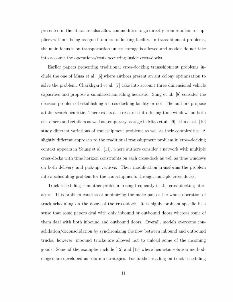
presented in the literature also allow commodities to go directly from retailers to sup-

pliers without being assigned to a cross-docking facility. In transshipment problems,

the main focus is on transportation unless storage is allowed and models do not take

into account the operations/costs occurring inside cross-docks.

Earlier papers presenting traditional cross-docking transshipment problems in-

clude the one of Musa et al. [6] where authors present an ant colony optimization to

solve the problem. Charkhgard et al. [7] take into account three dimensional vehicle

capacities and propose a simulated annealing heuristic. Sung et al. [8] consider the

decision problem of establishing a cross-docking facility or not. The authors propose

a tabu search heuristic. There exists also research introducing time windows on both

customers and retailers as well as temporary storage in Miao et al. [9]. Lim et al. [10]

study different variations of transshipment problems as well as their complexities. A

slightly different approach to the traditional transshipment problem in cross-docking

context appears in Yeung et al. [11], where authors consider a network with multiple

cross-docks with time horizon constraints on each cross-dock as well as time windows

on both delivery and pick-up vertices. Their modification transforms the problem

into a scheduling problem for the transshipments through multiple cross-docks.

Truck scheduling is another problem arising frequently in the cross-docking liter-

ature. This problem consists of minimizing the makespan of the whole operation of

truck scheduling on the doors of the cross-dock. It is highly problem specific in a

sense that some papers deal with only inbound or outbound doors whereas some of

them deal with both inbound and outbound doors. Overall, models overcome con-

solidation/deconsolidation by synchronizing the flow between inbound and outbound

trucks; however, inbound trucks are allowed not to unload some of the incoming

goods. Some of the examples include [12] and [13] where heuristic solution method-

ologies are developed as solution strategies. For further reading on truck scheduling

11

in cross-docks, we refer to Belle et al. [1].

Dock-door assignment problems deal with a single cross-dock in which a set of

origin and a set of destination points must be assigned to inbound and outbound

doors, respectively, of the cross-docking facility. In contrast to transshipment prob-

lems, cost occurs not because of the transportation cost in-between customers and

cross-dock or in-between suppliers and cross-dock but because of the transportation

of the goods inside the cross-docking facility. In other words, the cost associated is

that of transporting the goods from inbound doors to outbound doors. Generally,

authors prefer to use the number of trips made between inbound and outbound doors

and the distance as a measure of the handling costs. We note that this problem is

closely related to our problem where the origins are assigned to inbound doors and

the cost is the transportation cost incurred by transporting goods from inbound to

outbound doors.

One of the first papers concerning cross-dock door assignment problem (Tsui et

al. [14]) introduces a bilinear model and proposes a heuristic methodology to solve

the problem. The authors first assign incoming shipments to outbound doors and op-

timize outgoing shipments and then repeat the same process by fixing either incoming

or outgoing shipments until the solution converges to a desired value. Computational

results are not provided. Hence, the efficiency of the proposed heuristics is unknown.

In [15], the same authors propose a branch and bound method to solve the same prob-

lem to optimality; however, their results show that as instances get fairly larger, CPU

time spent increases dramatically. Guignard et al. [16] develops a heuristic solution

methodology where generalized assignment problems are solved at every iteration in

order to construct feasible assignments for inbound and outbound doors, respectively.

Zhu et al. [17] modifies the quadratic assignment model proposed by Tsui et al. [14]

and transforms the model into a Generalized Quadratic 3-dimensional Assignment

12

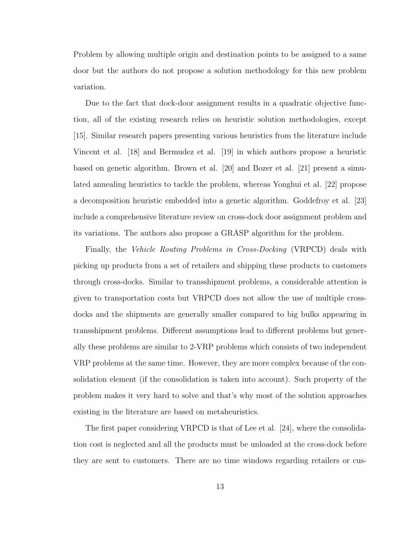
Problem by allowing multiple origin and destination points to be assigned to a same

door but the authors do not propose a solution methodology for this new problem

variation.

Due to the fact that dock-door assignment results in a quadratic objective func-

tion, all of the existing research relies on heuristic solution methodologies, except

[15]. Similar research papers presenting various heuristics from the literature include

Vincent et al. [18] and Bermudez et al. [19] in which authors propose a heuristic

based on genetic algorithm. Brown et al. [20] and Bozer et al. [21] present a simu-

lated annealing heuristics to tackle the problem, whereas Yonghui et al. [22] propose

a decomposition heuristic embedded into a genetic algorithm. Goddefroy et al. [23]

include a comprehensive literature review on cross-dock door assignment problem and

its variations. The authors also propose a GRASP algorithm for the problem.

Finally, the Vehicle Routing Problems in Cross-Docking (VRPCD) deals with

picking up products from a set of retailers and shipping these products to customers

through cross-docks. Similar to transshipment problems, a considerable attention is

given to transportation costs but VRPCD does not allow the use of multiple cross-

docks and the shipments are generally smaller compared to big bulks appearing in

transshipment problems. Different assumptions lead to different problems but gener-

ally these problems are similar to 2-VRP problems which consists of two independent

VRP problems at the same time. However, they are more complex because of the con-

solidation element (if the consolidation is taken into account). Such property of the

problem makes it very hard to solve and that’s why most of the solution approaches

existing in the literature are based on metaheuristics.

The first paper considering VRPCD is that of Lee et al. [24], where the consolida-

tion cost is neglected and all the products must be unloaded at the cross-dock before

they are sent to customers. There are no time windows regarding retailers or cus-

13

tomers but the authors consider a maximum time limit so that the whole process must

be completed before. Simultaneous arrival of the vehicles at the cross-dock after the

pick-up process is assumed. A tabu search based metaheuristic is proposed to solve

the corresponding problem. The authors solve instances with up to 50 vertices and

compare the results with the optimal solutions found by enumeration. In a general

sense, this paper treats VRPCD as a pick-up and delivery problem in the presence

of a cross-dock. Liao et al. [25] consider the same problem as of Lee et al. but they

propose a new Tabu Search scheme that proves to be better than that of Lee et al..

Wen et al. [26] present the first attempt at considering the consolidation of prod-

ucts at the cross-dock in VRPCD. Their model consists of commodities with fixed

origin and destination points. Vehicles must serve these origins and destinations by

respecting their time windows. Consolidation is tackled only in a way that when a

commodity is unloaded at the cross-dock, it has to be loaded to another vehicle that

is serving the destination of that commodity. However, all costs of consolidation are

neglected. The authors propose a Tabu Search metaheuristic with an adaptive mem-

ory procedure for the problem. Tarantilis [27] develops another heuristics based on an

adaptive multi-start tabu search for the problem proposed by Wen et al. and this new

heuristic outperforms the one proposed before. In addition, the author considers an

open network VRPCD where vehicles do not necessarily depart from the cross-dock.

Similarly, Petersen et al. [28] propose a VRPCD application with time windows with

both pick-ups and deliveries and they develop a large neighborhood search heuristic

to solve the problem. Dondo et al. [29] propose a model of VRPCD without time

windows. In this paper, it is assumed that the inbound and outbound doors are suf-

ficient to serve all the vehicles at the same time (infinite number of doors). Similar

to Tarantilis et al. and Wen et al., vehicles unload the requests at the cross-dock

only if a different vehicle would serve the destination point of an order. On the other

14

hand, two different objective functions were introduced, the first one minimizing the

total cost and the second one minimizing the makespan (operational time of the latest

vehicle). They used the sweep-based heuristic proposed by Gillett and Miller (1974)

and they are able to solve instances containing up to 50 customers.

Agustina et al. [30] propose a model that combines truck scheduling on the in-

bound and outbound doors, product consolidation, temporary storage and routing

from the outbound doors to customers. There is no cost associated with the consoli-

dation of the orders (products); however, loading and unloading of the pallets is taken

into account and is integrated with the time windows on the customers. On the other

hand, supplier time windows are neglected and the arrival time of the trucks (after

pick-up process) is assumed to be known. Similar to previous papers considering

VRPCD, inbound and outbound door capacities have not been taken into account

but the number of inbound and outbound doors is known and limited as well as the

temporary storage area. Overall, the problem tries to find a solution to two truck

scheduling problems (one on inbound doors and one on outbound doors without any

capacities on the doors) and a VRP from outbound doors to customers with time win-

dows and temporary holding. The authors do not propose a solution methodology for

the problem but they present preliminary experiments for a very small problem in-

stance with CPLEX. Even though there is no efficient solution methodology proposed

for this problem, Agustina et al.’s work is important for cross-docking literature in a

way that it combines three different problems, truck scheduling, allocation and VRP.

Santos et al. propose two different set partitioning reformulations for VRPCD

[31] and [32]. These two papers are the only ones so far presenting exact solution

methodologies for VRPCD problem. Santos et al. [31] has different types of variables

for routes visiting suppliers and customers, and an unloading cost is incurred whenever

a vehicle picks up a delivery but does not carry it to the corresponding customer. This

15

is achieved by forcing decision variables of loading/unloading if such operation occurs.

The second model proposed by the same authors tackles all the routings with only

one type of variable and similarly an unloading/loading decision is introduced. Both

models impose consolidation as well as full loading/unloading of the goods. However,

door capacities and flow costs occurring inside the cross-dock are neglected. Their

second model provides better lower bounds than the first one for most of the instances

but its computational complexity proves to be higher than the first one as CPU times

increase significantly for instances with 30 or more vertices.

Most articles in VRPCD deal with a distribution system through a single cross-

docking facility. However, some authors have studied the VRPCD with multiple

cross-docks. For example, Dondo et al. [33] presents the multi-echelon vehicle routing

problem with cross-docking where the distribution of the goods from factories to

customers are achieved through multiple cross-docks in such a way that vehicles may

or may not stop by a cross-dock. In a manner, such problems recall a transshipment

problem. Unlike previous works, models include routings instead of assignments. We

refer to Feliu et al. [34] for a review and a comparative analysis of multi-echelon and

single-echelon vehicle routing problems with cross-docking.

16

3 The Dock-Door Assignment and

Vehicle Routing Problem

In this chapter we first introduce the formal definition of the Dock-Door Assign-

ment and Vehicle Routing Problem. We then present five different mixed integer

programming formulations for the problem and describe potential applications for it.

3.1 Problem Definition

Let G = (V,A) be a graph where V denotes the set of vertices and A denotes the

set of arcs. Let I ⊂ V and J ⊂ V be the subsets of vertices representing, respectively,

the inbound and outbound doors such that I ∩ J = ∅. Furthermore, let M ⊂ V be

a subset of vertices representing the origin points (suppliers) and N ⊂ V be another

subset representing the destination points (customers) such that M ∩ N = ∅. In

addition, I ∩M = ∅, I ∩N = ∅, J ∩M = ∅, and J ∩N = ∅ .

We introduce four set of arcs such that A1∪A2∪A3∪A4 = A .The first set A1 ⊂ A

represents the arcs (m, i) ∈M × I connecting each pair of origin points and inbound

doors. The second set A2 ⊂ A denotes the arcs (i, j) ∈ I × J connecting each pair of

inbound and outbound doors. The third set A3 ⊂ A represents the arcs (j, a) ∈ J×N

connecting the outbound doors with every destination vertex. Finally, the fourth set

A4 ⊂ A denote the arcs (a, b) ∈ N ×N connecting each pair of destinations. Finally,

let K be the set of commodities where for each k ∈ K, let o(k) ∈ M and d(k) ∈ N

denote the origin and the destination of the commodity, respectively, and let qk be

the quantity of the commodity.

17

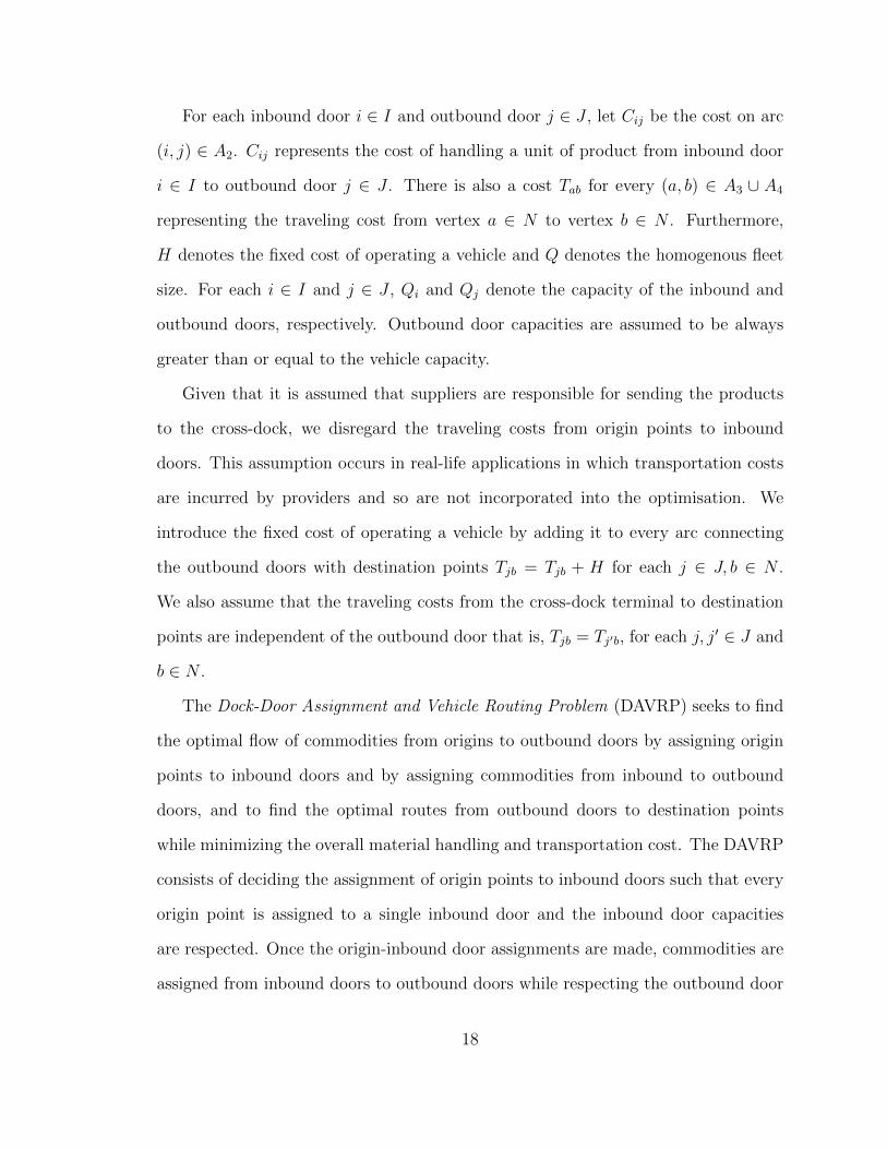
For each inbound door i ∈ I and outbound door j ∈ J , let Cij be the cost on arc

(i, j) ∈ A2. Cij represents the cost of handling a unit of product from inbound door

i ∈ I to outbound door j ∈ J . There is also a cost Tab for every (a, b) ∈ A3 ∪ A4

representing the traveling cost from vertex a ∈ N to vertex b ∈ N . Furthermore,

H denotes the fixed cost of operating a vehicle and Q denotes the homogenous fleet

size. For each i ∈ I and j ∈ J , Qi and Qj denote the capacity of the inbound and

outbound doors, respectively. Outbound door capacities are assumed to be always

greater than or equal to the vehicle capacity.

Given that it is assumed that suppliers are responsible for sending the products

to the cross-dock, we disregard the traveling costs from origin points to inbound

doors. This assumption occurs in real-life applications in which transportation costs

are incurred by providers and so are not incorporated into the optimisation. We

introduce the fixed cost of operating a vehicle by adding it to every arc connecting

the outbound doors with destination points Tjb = Tjb + H for each j ∈ J, b ∈ N .

We also assume that the traveling costs from the cross-dock terminal to destination

points are independent of the outbound door that is, Tjb = Tj′b, for each j, j′ ∈ J and

b ∈ N .

The Dock-Door Assignment and Vehicle Routing Problem (DAVRP) seeks to find

the optimal flow of commodities from origins to outbound doors by assigning origin

points to inbound doors and by assigning commodities from inbound to outbound

doors, and to find the optimal routes from outbound doors to destination points

while minimizing the overall material handling and transportation cost. The DAVRP

consists of deciding the assignment of origin points to inbound doors such that every

origin point is assigned to a single inbound door and the inbound door capacities

are respected. Once the origin-inbound door assignments are made, commodities are

assigned from inbound doors to outbound doors while respecting the outbound door

18

capacities. Finally, vehicle routing decisions are considered for sending the commodi-

ties from outbound doors to the corresponding destination points while respecting

the vehicle capacities.

Figure 4 depicts a graphical representation of a possible solution to the DAVRP

for an instance with four suppliers, eight commodities, two inbound and outbound

doors and six customers.

I1

J2J1

I2

M1

N2

M4M3

N1

M2

N4

N5

N6N3

o(k1)=o(k2)=M1o(k3)=o(k4)=M2

o(k5)=o(k6)=M3o(k7)=o(k8)=M4

d(k2)=d(k3)=N2

d(k1)=N1d(k5)=N3 d(k4)=d(k8)=N6

d(k7)=N5

d(k6)=N4

Figure 4: Graphical Representation of a DAVRP instance.

In Figure 4, commodity 4 follows path M2−I1−J2−N4−N5−N6 and commodity

8 follows the path M4− I2− J2−N4−N5−N6. These two commodities originate at

19

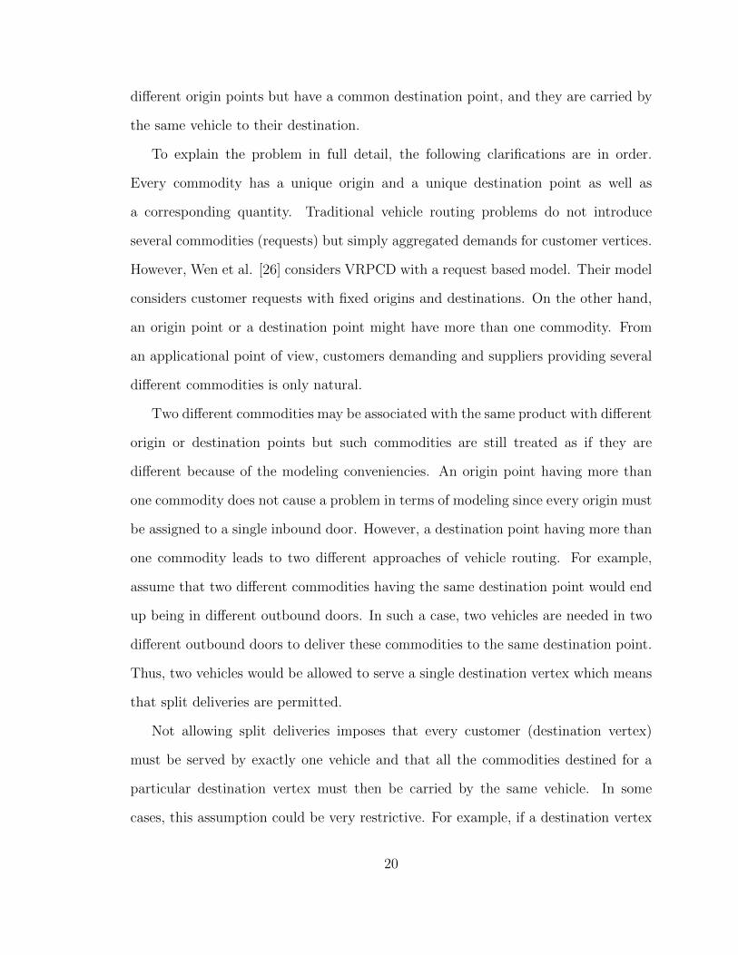
different origin points but have a common destination point, and they are carried by

the same vehicle to their destination.

To explain the problem in full detail, the following clarifications are in order.

Every commodity has a unique origin and a unique destination point as well as

a corresponding quantity. Traditional vehicle routing problems do not introduce

several commodities (requests) but simply aggregated demands for customer vertices.

However, Wen et al. [26] considers VRPCD with a request based model. Their model

considers customer requests with fixed origins and destinations. On the other hand,

an origin point or a destination point might have more than one commodity. From

an applicational point of view, customers demanding and suppliers providing several

different commodities is only natural.

Two different commodities may be associated with the same product with different

origin or destination points but such commodities are still treated as if they are

different because of the modeling conveniencies. An origin point having more than

one commodity does not cause a problem in terms of modeling since every origin must

be assigned to a single inbound door. However, a destination point having more than

one commodity leads to two different approaches of vehicle routing. For example,

assume that two different commodities having the same destination point would end

up being in different outbound doors. In such a case, two vehicles are needed in two

different outbound doors to deliver these commodities to the same destination point.

Thus, two vehicles would be allowed to serve a single destination vertex which means

that split deliveries are permitted.

Not allowing split deliveries imposes that every customer (destination vertex)

must be served by exactly one vehicle and that all the commodities destined for a

particular destination vertex must then be carried by the same vehicle. In some

cases, this assumption could be very restrictive. For example, if a destination vertex

20

n has a demand of several commodities and the vehicle capacity is respectively low

compared to the accumulated demand of that destination vertex, it may happen that

a vehicle would leave the cross-dock, serve destination vertex n and return to the

cross-dock. Such restriction would end up causing high vehicle operation costs. It

may also happen that the cumulated demand of a customer n is above the vehicle

capacity in which case the problem becomes infeasible. On the other hand, if this

particular vertex n has small amounts of several different commodities, it may be

better in terms of cost to allow several vehicles to visit a single vertex, each vehicle

carrying a different commodity destined for the same vertex. Thus, we propose to

have both approaches, one where the split deliveries are allowed and the other where

the whole demand of every customer must be carried by exactly one vehicle. The

latter requires the assumption that vehicle capacities will always be greater than

or equal to the demand of the customer with the highest demand; however, split

deliveries only assumes that the vehicle capacities must be greater than or equal to

the quantity of the commodity with the largest amount.

In order to represent both cases with one model, we simply need to perform a

pre-processing on the destination vertices. When solving the split deliveries case,

destination vertices are duplicated in such a way that there is a destination vertex for

every single commodity in the network. The number of destination vertices becomes

equal to the number of commodities and the cost of traveling from a destination

vertex a ∈ N to the corresponding duplicated vertex a′ ∈ N becomes equal to zero.

Duplication of destination vertices brings flexibility in terms of modeling. The math-

ematical formulations that are presented next are valid for both slit deliveries and

non-split deliveries by performing the above mentioned procedure. However, dupli-

cating vertices increase the size of the instances and this changes the solution time of

the problem.

21

Allowing split deliveries not only brings flexibility for the routing but also for

the consolidation. Not allowing split deliveries forces commodities with common

destinations to end up at the same outbound door regardless of which inbound door

they are coming from. Figure 5 depicts a case where split deliveries are allowed. In

this figure, the number of destination vertices are equal to the number of commodities

in the network. N ′2 and N ′6 are the duplicated vertices for N2 and N6, respectively.

I1

J2J1

I2

M1

N2

M4M3

N1

M2

N4

N5

N6N3

N2'

N6'

d(k2)=N2'

d(k8)=N6'

o(k1)=o(k2)=M1 o(k3)=o(k4)=M2

o(k5)=o(k6)=M3o(k7)=o(k8)=M4

d(k3)=N2d(k1)=N1

d(k5)=N3

d(k4)=N6

d(k7)=N5

d(k6)=N4

Figure 5: Split deliveries allowed.

In Figure 5, commodity 4 follows the path M2 − I1 − J1 − N1 − N ′2 − N6 and

commodity 8 follows the path M4−I2−J2−N2−N5−N4−N ′6. In contrast to Figure

22

4, these commodities are carried by two different vehicles. Similarly, commodities 2

and 3 are carried by two different vehicle even if they have a common destination.

Note that the split delivery approach does not allow a single commodity to be

broken down into smaller quantities. Following Figure 5 as an example, even though

customer 2 is served by two different vehicles, commodities 2 and 3 are shipped as

a whole and half of commodity 2 cannot be served by the vehicle departing from

outbound door 2. In real life, split deliveries gives the decision maker the possibility

to balance the trade-off between full truck load and less-than truck load shipments.

The cost considered in the model contains the material handling cost of commodi-

ties inside the cross-dock and the transportation cost from cross-dock to customers.

There is no cost associated with the assignment of suppliers to inbound doors. In

some applications, suppliers are not part of the logistic provider that is responsible

of the cross-dock and hence, the transportation cost of the products from supplier to

the cross-dock is either being paid by the supplier or they have a fixed transportation

cost. Moreover, assigning an incoming vehicle to different inbound doors will have

an effect on the cost of consolidation, not on the cost of transporting the goods from

suppliers to the cross-dock.

3.2 Mathematical Programming Formulations

In this section, we present five different mathematical formulations based on dif-

ferent existing formulations of capacitated vehicle routing problems. The first model

incorporates rounded capacity constraints. The second one is based on a single com-

modity flow formulation presented by Baldacci et al. [35], the third one is based on

a multi commodity flow formulation first presented by Gavin et al. [36], and the

last one is based on the Miller-Tucker-Zemlin inequalities first proposed for the Trav-

23

eling Salesman Problem [37]. It is known that different formulations may provide

different lower bounds associated with their linear programming relaxations. In the

computational results section, we discuss the performance of these formulations.

We define the following sets of decision variables: binary variables Xmi,m ∈

M, i ∈ I denoting the assignment of origin points to inbound doors, binary variables

Yijk, i ∈ I, j ∈ J, k ∈ K denoting the assignment of commodities from inbound doors

to outbound doors, and binary variables Zabj, a, b ∈ N, j ∈ N denoting the routes

associated with outbound doors.

Input Data:

I: Set of inbound doorsJ : Set of outbound doorsK: Set of commoditiesM : Set of origin verticesN : Set of destination verticeso(k): Origin of commodity kd(k): Destination of commodity kqk : Quantity of commodity kCij : Unit handling cost from inbound door i to outbound door jTab : Transportation cost from destination vertex a to vertex bQi : Capacity of inbound door iQj : Capacity of outbound door jQ : Capacity of a vehicle

Decision Variables:

Xmi :

1 if origin vertex m is assigned to inbound door i0 otherwise

Yijk :

1 if commodity k is routed from inbound door i to outbound door j0 otherwise

Zabj :

1 if a vehicle associated with the outbound door j travels

from vertex a to vertex b0 otherwise.

24

3.2.1 Natural Three Index Formulation (F1)

Using decision variables Xmi, Yijk, and Zabj, the DAVRP can be stated as follows:

(F1) Minimize∑k∈K

∑j∈J

∑i∈I

CijqkYijk +∑j∈J

∑b∈N∪J

∑a∈N∪J

TabZabj (1)

Subject to∑i∈I

Xmi = 1 ∀m ∈M (2)

Xo(k)i =∑j∈J

Yijk ∀i ∈ I,∀k ∈ K (3)

∑k∈K

∑j∈J

qkYijk ≤ Qi ∀i ∈ I (4)

∑a∈N∪J

Zad(k)j =∑i∈I

Yijk ∀j ∈ J,∀k ∈ K (5)∑j∈J

∑b∈N∪J

Zabj = 1 ∀a ∈ N (6)

∑a∈N∪J

Zanj −∑

a∈N∪JZnaj = 0 ∀n ∈ N ∪ J,∀j ∈ J (7)∑

j∈J

∑b/∈S

∑a∈S

Zabj ≥∑

k:d(k)∈Sdqk/Qe ∀S, S ⊂ N ∪ J, 2 ≤ |S| ≤ |N ∪ J | (8)

∑k∈K

∑a∈N∪J

qkZad(k)j ≤ Qj ∀j ∈ J (9)

Zabj ∈ 0, 1 ∀a ∈ N ∪ J, b ∈ N ∪ J,∀j ∈ J (10)

Yijk ∈ 0, 1 ∀i ∈ I, j ∈ J, k ∈ K (11)

Xmi ∈ 0, 1 ∀m ∈M, ∀i ∈ I. (12)

The objective function minimizes the cost occurring due to the flow of goods

from inbound doors to outbound doors and the transportation cost of the goods from

outbound doors to customers as well as operational cost of vehicles. From a general

perspective, constraints (2)-(4) model the assignment of suppliers (origin vertices)

to inbound doors and the routing of commodities from inbound to outbound doors.

Constraints (6)-(9) model the vehicle routes while constraints (5) link the assignment

25

and routes to ensure that the commodities are in their corresponding outbound door

to be delivered to their destinations.

More specifically, constraints (2) are the degree constraints imposing that every

supplier vertex m must be assigned to an inbound door i. Constraints (3) denote

that if an origin vertex m is assigned to an inbound door i, then all the commodities

coming from that origin vertex must be handled through inbound door i and must

be assigned to an outbound door. Constraints (4) are the capacity constraints for

inbound doors. Constraints (5) are the linking constraints ensuring that exactly one

of the vehicles leaving the inbound door j travels to the destination of a commodity

k, if that commodity is assigned to the outbound door j.

Constraints (6) force every customer n ∈ N to be served exactly once, flow con-

servation constraints (7) denote that if a vehicle is entering a vertex, it must also

leave the vertex, and the rounded capacity constraints (8) make sure that all the

vehicles leave and come back to cross-dock, that there will be no subtours and that

the vehicle capacities will be respected. Note that the set (8) contains an exponential

number of constraints. The last constraint set (9) are the outbound door capacity

constraints denoting that the vehicles associated with an outbound door j cannot

have a cumulated carriage larger than the capacity of that outbound door. Finally

constraints (10)-(12) impose integrality conditions on the variables.

3.2.2 Single Commodity Flow Formulation (F2)

The second formulation is based on the Single Commodity Flow Formulation

presented by Baldacci et al. [35] for the Capacitated Vehicle Routing Problem. We

define continuous decision variables Uab, a, b ∈ N ∪ J determining the quantity of

products sent from vertex a to vertex b. We define the total demand of destination

26

points as Dn =∑

k∈K:d(k)=n qk. Using the decision variables Xmi, Yijk, Zabj, and

continuous decision variables Uab, we restate the DAVRP as follows:

(F2) Minimize∑k∈K

∑j∈J

∑i∈I

CijqkYijk +∑j∈J

∑b∈N∪J

∑a∈N∪J

TabZabj (13)

Subject to∑i∈I

Xmi = 1 ∀m ∈M (14)

Xo(k)i =∑j∈J

Yijk ∀i ∈ I,∀k ∈ K (15)

∑k∈K

∑j∈J

qkYijk ≤ Qi ∀i ∈ I (16)

∑a∈N∪J

Zad(k)j =∑i∈I

Yijk ∀j ∈ J,∀k ∈ K (17)∑j∈J

∑b∈N∪J

Zabj = 1 ∀a ∈ N (18)

∑a∈N∪J

Zanj −∑

a∈N∪JZnaj = 0 ∀n ∈ N, ∀j ∈ J (19)∑

k∈K

∑a∈N∪J

qkZad(k)j ≤ Qj ∀j ∈ J (20)∑a∈N∪J

Uab −∑

a∈N∪JUba = Db ∀b ∈ N (21)

Uab ≤ Q∑j∈J

Zabj ∀a ∈ N ∪ J,∀b ∈ N ∪ J (22)

Zabj ∈ 0, 1 ∀a ∈ N ∪ J, b ∈ N ∪ J,∀j ∈ J (23)

Yijk ∈ 0, 1 ∀i ∈ I, j ∈ J, k ∈ K (24)

Xmi ∈ 0, 1 ∀m ∈M, ∀i ∈ I (25)

Uab ∈ R+ ∀a ∈ N ∪ J, b ∈ N ∪ J. (26)

The objective function (13) and the constraints (14)-(20) are the same as (1)-

(7) and (9). Similarly, the integrality constraints (23)-(25) do not change and non

negativity conditions on new new variables are imposed by (26). Instead of rounded

capacity constraints (8), constraints (21)-(22) are introduced imposing, respectively,

27

flow conservation on arcs and vehicle capacities. These two new constraint sets (21)-

(22) eliminate sub tours and impose vehicle capacities. Rounded capacity constraints

(8) are exponential in number and by using (21)-(22) instead, we are able to reduce

the number of constraints. However, number of decision variables is increased.

3.2.3 Multi Commodity Flow Formulation (F3)

We formulate the DAVRP by using an adaptation of the Multi Commodity Flow

Formulation first proposed by Gavin et al. [36] in an oil delivery problem. New

decision variables Rabl, a, b ∈ N ∪ J, l ∈ N are introduced. Rabl are the flow variables

specifying the amount of demand destined to customer l ∈ N that is transported

from vertex a to vertex b. Using the decision variables Xmi, Yijk, Zabj and Rabl, the

DAVRP can be stated as follows:

(F3) Minimize∑k∈K

∑j∈J

∑i∈I

CijqkYijk +∑j∈J

∑b∈N∪J

∑a∈N∪J

TabZabj (27)

Subject to∑i∈I

Xmi = 1 ∀m ∈M (28)

Xo(k)i =∑j∈J

Yijk ∀i ∈ I,∀k ∈ K (29)

∑j∈J

∑k∈K

qkYijk ≤ Qi ∀i ∈ I (30)

∑a∈N∪J

Zad(k)j =∑i∈I

Yijk ∀j ∈ J,∀k ∈ K (31)∑j∈J

∑b∈N∪J

Zabj = 1 ∀a ∈ N (32)

∑a∈N∪J

Zanj −∑

a∈N∪JZnaj = 0 ∀n ∈ N, ∀j ∈ J (33)∑

k∈K

∑a∈N∪J

qkZad(k)j ≤ Qj ∀j ∈ J (34)∑a∈N∪J

Rabl −∑

a∈N∪JRbal = Dl ∀l ∈ N, b = l (35)

28

∑a∈N∪J

Rabl −∑

a∈N∪JRbal = 0 ∀l ∈ N, b 6= l, b ∈ N (36)∑

b∈J

∑a∈N∪J

Rabl −∑

a∈N∪J

∑b∈J

Rbal = −Dl ∀l ∈ N (37)∑l∈N

∑b∈N∪J

Rabl ≤ (Q−Da)∑j∈J

∑b∈N∪J

Zabj ∀a ∈ N ∪ J (38)

Rabl ≤ Dl

∑j∈J

Zabj ∀l ∈ N,∀a, b ∈ N ∪ J (39)

Zabj ∈ 0, 1 ∀a ∈ N ∪ J, b ∈ N ∪ J,∀j ∈ J (40)

Yijk ∈ 0, 1 ∀i ∈ I, j ∈ J, k ∈ K (41)

Xmi ∈ 0, 1 ∀m ∈M,∀i ∈ I (42)

Rabl ∈ R+ ∀a ∈ N ∪ J, b ∈ N ∪ J,∀l ∈ N. (43)

The objective function (27) and the constraints (28)-(34) are the same as (1)-

(7) and (9). Constraints (35)-(37) are commodity flow constraints guaranteeing that

the demand of each vertex is satisfied. Constraints (38) denote the available vehicle

capacities after a vehicle visits a vertex. Constraints (39) are the capacity constraints

on arcs forcing the flow destined for vertex l to be always smaller than or equal to

the demand of vertex l. F3 replaces constraints (8) by introducing the constraints

(35)-(39). Finally, constraints (43) impose non negativity conditions on the new set

of variables.

3.2.4 Miller-Tucker-Zemlin Based Formulation (F4)

We define the new set of variables Wa for every destination point a ∈ N denoting

the total demand on the trip of a vehicle till vertex a (including vertex a). Using the

decision variables Xmi, Yijk, Zabj and Wa, we state the DAVRP as follows:

(F4) Minimize∑k∈K

∑j∈J

∑i∈I

CijqkYijk +∑j∈J

∑b∈N∪J

∑a∈N∪J

TabZabj (44)

29

Subject to∑i∈I

Xmi = 1 ∀m ∈M (45)

Xo(k)i =∑j∈J

Yijk ∀i ∈ I,∀k ∈ K (46)

∑j∈J

∑k∈K

qkYijk ≤ Qi ∀i ∈ I (47)

∑a∈N∪J

Zad(k)j =∑i∈I

Yijk ∀j ∈ J,∀k ∈ K (48)∑j∈J

∑b∈N∪J

Zabj = 1 ∀a ∈ N (49)

∑a∈N∪J

Zanj −∑

a∈N∪JZnaj = 0 ∀n ∈ N ∪ J,∀j ∈ J (50)∑

a∈N∪J

∑k∈K

qkZad(k)j ≤ Qj ∀j ∈ J (51)

Wa −Wb +Q∑j∈J

Zabj ≤ Q−Db ∀a ∈ N, a 6= b (52)

Da ≤ Wa ≤ Q ∀a ∈ N (53)

Zabj ∈ 0, 1 ∀a ∈ N ∪ J, b ∈ N ∪ J,∀j ∈ J (54)

Yijk ∈ 0, 1 ∀i ∈ I, j ∈ J, k ∈ K (55)

Xmi ∈ 0, 1 ∀m ∈M,∀i ∈ I (56)

Wa ∈ R+ ∀a ∈ N. (57)

F4 is based on eliminating subtours by using the so-called Miller-Tucker-Zemlin

inequalities. These were first proposed by Miller, Tucker and Zemlin [37] for the

Traveling Salesman Problem. The objective function (44) and the constraints (45)-

(51) are directly taken from F1. Constraints (52) impose subtour elimination and

vehicle capacities conditions. Constraints (53) are the upper and lower bounds on

the total quantity of products carried on a trip.

3.2.5 Set Partitioning Formulation (F5)

The next formulation is based on the well-known set partitioning reformulation

of the CVRP introduced in [35]. This type of formulation is known to provide strong

30

linear programming relaxation bounds for various VRPs but requires the use of ad-

hoc solution algorithms to handle the huge number of variables required to model the

problem.

For each inbound door i ∈ I, let ΩPi be the set containing all the feasible as-

signment patterns for inbound door i. Assignment patterns for each i ∈ I define

structures such that several origin points m ∈M are assigned to the inbound door i,

and the commodities originating at these origin points k ∈ K : o(k) = m are assigned

from inbound door i to outbound doors j ∈ J while respecting the capacity Qi of the

inbound door i. Let Cpi be the cost of an assignment pattern p ∈ ΩP

i . Figure 6 and

Figure 7 depict two different possible assignment patterns for an inbound door.

I1

J3J1

M1 M2

o(k1)=o(k2)=M1 o(k3)=o(k4)=M2

J2

k1,k2 k3,k4

Figure 6: Assignment pattern example 1.

In the pattern given in Figure 6, commodities 1 and 2 follow path M1 − I1 − J1,

31

and commodities 3 and 4 follow path M2− I1−J3. In Figure 7, commodities 1 and 3

follow the same path as of Figure 6 but commodities 2 and 4 follow paths M1−I1−J2

and M2 − I1 − J2, respectively.

I1

J3J1

M1 M2

o(k1)=o(k2)=M1 o(k3)=o(k4)=M2

J2

k1 k3

k2,k4

Figure 7: Assignment pattern example 2.

For each outbound door j ∈ J , let ΩRj be the set containing all the feasible routes

for outbound door j. Feasible routes define structures such that a vehicle leaves the

cross-dock from door j, performs a route visiting some customers while respecting the

vehicle capacity and subtour elimination constraints, and comes back to cross-dock

at door j by the end of the operation. Let Crj be the cost of a route r ∈ Ωr

j .

For every customer n ∈ N , let Dn =∑

k∈K:d(k)=n qk be the total demand of the

customer. For every supplier m ∈ M , let Om =∑

k∈K:o(k)=m qk be the total quantity

of goods originating at that supplier. Finally, let us introduce the binary constants:

32

apmi defining the supplier-inbound door assignment, hpijk defining the commodity as-

signment from inbound door i to outbound door j in assignment an pattern p ∈ ΩPi ,

and brnj defining a route r ∈ ΩRj . We define binary decision variables λrj and θpi for

routes and assignments, respectively.

Input Data:

ΩPi : Set of assignment patterns associated with inbound door i

ΩRj : Set of routes associated with outbound door j

Cpi : Handling cost of assignment p

Crj : Routing cost of route r

Dn : Total demand of customer nOm: Total quantity of commodities originated in mqk: Quantity of commodity k

apmi :

1 if origin vertex m is assigned to inbound door i

in the assignment patern p0 otherwise

hpijk :

1 if commodity k is assigned from inbound door i to outbound door j

in the assignment pattern p0 otherwise

brnj :

1 if route r is associated with the outbound door j

and serves the destination vertex n0 otherwise

grabj :

1 if route r associated with the outbound door j

and travels from vertex a to vertex b0 otherwise

Decision Variables:

λrj :

1 if route r associated with outbound door j is selected0 otherwise

θpi :

1 if assignment pattern p associated with inbound door i is selected0 otherwise.

33

Using decision variables λrj and θpi , the DAVRP can be stated as follows:

(F5) Minimize∑i∈I

∑p∈ΩP

i

Cpi θ

pi +

∑j∈J

∑r∈ΩR

j

Crjλ

rj (58)

Subject to∑i∈I

∑p∈ΩP

i

apmiθpi = 1 ∀m ∈M (59)

∑p∈ΩP

i

θpi ≤ 1 ∀i ∈ I (60)

∑i∈I

∑p∈ΩP

i

hpijkθpi −

∑r∈ΩR

j

brd(k)jλrj = 0 ∀j ∈ J,∀k ∈ K (61)

∑j∈J

∑r∈ΩR

j

λrjbrnj = 1 ∀n ∈ N (62)

∑r∈ΩR

j

(∑n∈N

Dnbrnj)λ

rj ≤ Qj ∀j ∈ J (63)

λrj ∈ 0, 1 ∀r ∈ ΩRj ,∀j ∈ J (64)

θpi ∈ 0, 1 ∀p ∈ ΩPi , ∀i ∈ I. (65)

The objective function aims at minimizing the total cost. Constraints (59) ensure

that every origin point is assigned to an inbound door, while constraints (60) make

sure that there is at most one assignment pattern containing each inbound door.

Similarly, constraints (62) denote that every customer must be visited exactly once

and constraints (63) ensure that outbound door capacities are respected. Finally,

constraints (61) are the linking constraints ensuring that if a commodity is assigned

to an outbound door j, then there must be a vehicle departing from j and visiting

the corresponding destination of the commodity.

Note that the set of assignments contains all the feasible assignments with respect

to inbound door capacities and the set of routes contain all the feasible routes leaving

the cross-dock, visiting a subset of customers and coming back to cross-dock with no

34

sub tours while respecting the vehicle capacity.

3.3 Applications

There are several cross-docking scenarios that are available for warehouse man-

agement. Depending on the role played in the supply chain, companies adopt the

type of cross-docking strategy that is applicable to their practice. The most com-

mon cross-docking strategies are retail cross-docking, manufacturing cross-docking

and transportation cross-docking. Other strategies and the combination of these ex-

ist in real life such as introducing temporary storage in the cross-dock; however, we

will focus on the strategy where the DAVRP is applicable.

Retail cross-docking is the most common application of cross-docking strategy. In

this type of cross-docking, the manufacturer delivers goods directly to the retailer

without any intermediaries involved. The retailer unloads the goods from inbound

trucks coming from several manufacturers at inbound doors and then sort, repack, and

immediately load the goods into outbound trucks. Finally, outbound trucks deliver

the goods to the consumers. 3rd party retailers generally operate under this type of

cross-docking strategy.

In retail cross-docking, transportation cost of an incoming shipment is either fixed,

since they include direct truck load shipments, or supplier is responsible of these in-

coming shipments. In the first case where the 3rd party retailer is responsible of the

incoming shipments, retailer pays the transportation cost of goods from manufactur-

ing facilities to cross-dock terminals. However, these transportation costs are fixed

since the shipments are direct. In the second case where manufacturer is responsible

of the incoming shipments, 3rd party retailer does not pay the transportation cost of

inbound trucks. When this is applicable, manufacturers include the transportation

35

cost on the price of the goods, which is also fixed. Moreover, from retailer’s point

of view, processing inbound shipments at different inbound doors does not lead to

changes in the cost of incoming shipments but in the cost of material handling in-

between inbound and outbound doors. Thus, 3rd party retailers are only exposed to

the costs occurring by material handling and distribution of goods from cross-dock

to consumers [38].

As the worlds largest retailer, Wal-Mart is considered a best-in-class company for

its supply chain management practices. Wal-Mart’s cross-docking practice is known

to be one of the most efficient implementations in supply chain management [39]. Wal-

Marts fleet is used to pick up goods directly from manufacturers warehouses, thus

eliminating intermediaries and increasing responsiveness. The use of trucks raises

transportation costs but is justified in terms of reduced inventory. Products brought

in by truck to distribution centers is sorted for delivery to stores within 24 hours.

Wal-Mart, a pioneer in the logistics technique of cross-docking shows a solid example

to the application of the DAVRP.

Existing dock-door assignment problems consider only the consolidation and mate-

rial handling cost, whereas classical VRP problems focus only on the transportation

cost for routing the products between the cross-dock terminal and the destination

points. The proposed DAVRP integrates these interrelated problems to jointly opti-

mize the material handling and transportation costs.

36

4 Solution Algorithms

In this section we introduce a column generation (CG) algorithm, based on the set

partitioning formulation introduced in Section 3.2.5, to obtain lower bounds on the

optimal solution value of the DAVRP. We first define the restricted master problem

and the pricing problem. We then discuss the solution strategies for efficiently solving

the pricing problem and present the overall CG algorithm. We also provide some

acceleration techniques for improving the behavior of the CG. Finally, we present a

branch and bound heuristic and a local neighborhood search heuristic that exploit the

information generated by CG to obtain feasible solutions in reasonable CPU times.

4.1 Column Generation

The fact that many linear programs are too large to consider all the variables

explicitly, have led researchers to look for efficient algorithms to solve large-scale

linear programs. Since most of the variables will be non-basic and have a value of

zero in the optimal solution, only a subset of variables needs to be considered in

practice when solving the problem. First proposed by Ford and Fulkerson [40] for a

maximal multi-commodity network flow problem, and by Dantzig and Wolfe [41] for

linear programming problems, CG has proven to be a powerful technique to solve the

problems with a huge number of variables. In particular, in the context of integer

programming CG can be used to solve huge LP relaxations to obtain lower bounds on

the optimal solution value. This methodology has been successfully applied to solve

many well-known integer problems such as the cutting stock problem, scheduling

37

problems and vehicle routing problems.

The main idea behind CG is to divide the LP relaxation of the considered MIP

problem, denoted as the master problem (MP), into two subproblems: a restricted

master problem (RMP) and a pricing problem (PP). Given the large number of

columns (or variables) in the MP, in practice one works with a small subset of columns

by using the RMP. At each iteration of the simplex method, we look for a non-basic

variable to price out and enter the basis. That is, in the PP given a vector of dual

variables associated with the optimal solution of the current RMP, we wish to find

the non-basic variable with the smallest reduced cost coefficient. If such variable has

a non-positive reduced cost coefficient, then the current solution of the RMP solves

the MP as well. Otherwise, we add to the RMP a column derived from the PP, and

repeat with re-optimizing the RMP.

In the rest of this chapter, we explain how we adapt the CG methodology for

solving the LP relaxation of the set partitioning formulation fo the DAVRP.

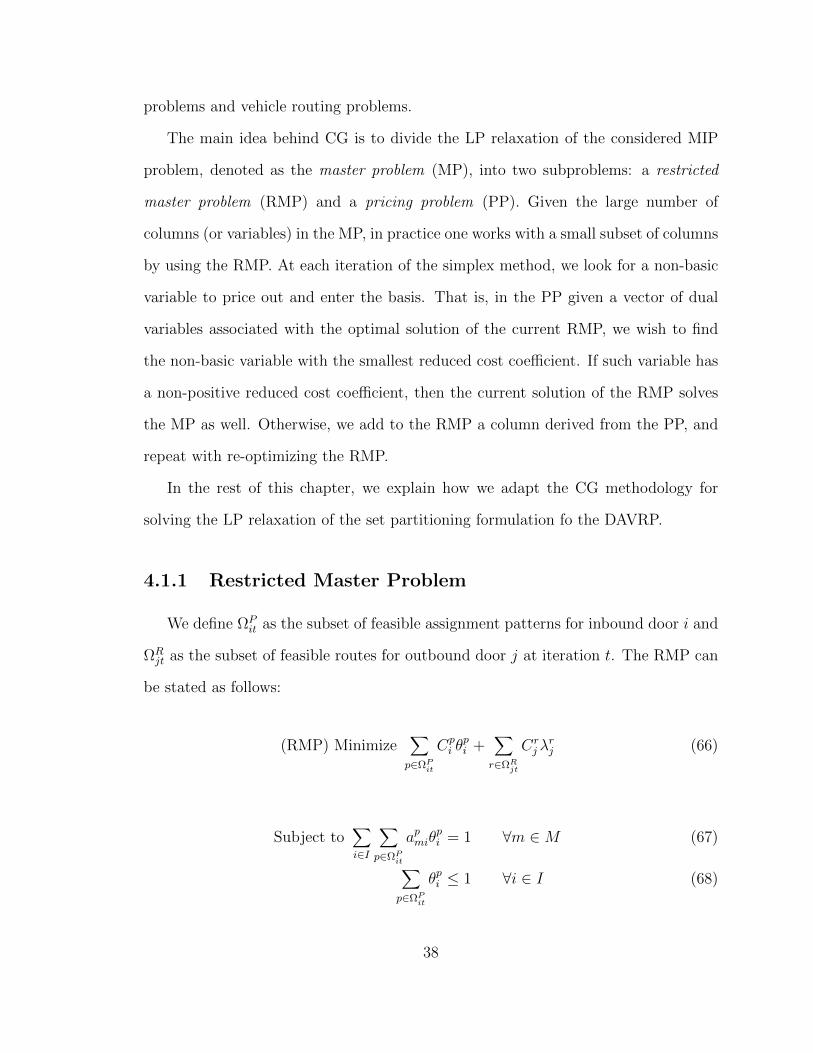
4.1.1 Restricted Master Problem

We define ΩPit as the subset of feasible assignment patterns for inbound door i and

ΩRjt as the subset of feasible routes for outbound door j at iteration t. The RMP can

be stated as follows:

(RMP) Minimize∑p∈ΩP

it

Cpi θ

pi +

∑r∈ΩR

jt

Crjλ

rj (66)

Subject to∑i∈I

∑p∈ΩP

it

apmiθpi = 1 ∀m ∈M (67)

∑p∈ΩP

it

θpi ≤ 1 ∀i ∈ I (68)

38

∑i∈I

∑p∈ΩP

it

hpijkθpi −

∑r∈ΩR

jt

brd(k)jλrj = 0 ∀j ∈ J,∀k ∈ K (69)

∑j∈J

∑r∈ΩR

jt

λrjbrnj = 1 ∀n ∈ N (70)

∑n∈N

∑r∈ΩR

jt

Dnbrnjλ

rj ≤ Qj ∀j ∈ J (71)

λrj ∈ R+ ∀r ∈ ΩRjt,∀j ∈ J (72)

θpi ∈ R+ ∀p ∈ ΩPit ,∀i ∈ I. (73)

Note that (66)-(73) is the LP relaxation of the set partitioning formulation with

only a small subset of the variables. This linear program can be efficiently solved by

using a general purpose solver (such as CPLEX).

4.1.2 Pricing Problem

We first introduce the dual variables associated with the constraints of the RMP.

In particular, let (α, µ, γ, β, π) be the vector of dual variables of appropriate dimension

associated with constraints (67)–(71), respectively. Then, the reduced cost coefficient

associated with inbound door i and assignment pattern p is

Cp

i =∑j∈J

∑k∈K

qkCijhpijk −

∑m∈M

αmapmi −

∑j∈J

∑k∈K

γjkhpijk − µi, (74)

and the reduced cost coefficient associated with outbound door j and a route r is

Crj =

∑a∈N∪J

∑b∈N∪J

Tabgrabj −

∑n∈N

βnbrnj −

∑n∈N

πjDnbrnj +

∑k∈K

γjkbrd(k)j. (75)

From (74) and (75), we note that the PP corresponds to the solution of two families

of independent subproblems, one for the variables associated with the assignments of

origins to inbound doors and the routing of commodities inside the cross-dock, and

39

another one for the variables associated with the routing of commodities between

outbound doors and destinations. For each i ∈ I, the corresponding assignment

subproblem should be able to identify assignments with a cost structure given in

(74) such that a subset of origins are assigned to inbound door i, while respecting

the capacity constraints of the door, and that all commodities associated with this

subset of origins are routed to exactly one outbound door. On the other hand, for

each j ∈ J the routing subproblem should be able to generate routes with the cost

structure of (75) such that the vehicle leaves the cross-dock from door j, visits a

subset of customers and comes back to cross-dock at door j, while respecting the

vehicle capacity and sub-tour elimination constraints.

For each i ∈ I, given an optimal dual vector (αt, µt, γt, βt, πt) of the RMP at

iteration t, the assignment subproblem can be stated as the following integer program:

Minimize∑j∈J

∑k∈K

qkCijhijk −∑m∈M

αtmami −

∑j∈J

∑k∈K

γtjkhijk − µti (76)

, Subject to∑m∈M

Omami ≤ Qi (77)∑j∈J

hijk = ao(k)i ∀k ∈ K (78)

ami ∈ 0, 1 ∀m ∈M (79)

hijk ∈ 0, 1 ∀j ∈ J,∀k ∈ K. (80)

Constraints (77) and (78) define a feasible assignment pattern associated with

inbound door i and these constraints, which are equivalent to constraints (3)–(4)

used in formulation F1. Constraints (79) and (80) impose integrality conditions on the

decision variables. In the next section we show how this problem can be transformed

into a pure 0-1 knapsack problem to efficiently solve it.

40

For each j ∈ J , given an optimal dual vector (αt, µt, γt, βt, πt) of the RMP at

iteration t, the routing subproblem can be stated as the following integer program:

Minimize∑

b∈N∪j

∑a∈N∪j

[Tab −

βta + βt

b

2−(Da +Db

2

)πtj

]gabj

+∑k′∈K

∑k∈K

(γtjk + γtjk′

2

)gd(k)d(k′)j (81)

Subject to∑b∈N

gjbj = 1 (82)∑a∈N

gajj = 1 (83)∑a∈N∪j

ganj −∑

a∈N∪jgnaj = 0 ∀n ∈ N ∪ j (84)

∑b∈N

∑a∈N∪j

Dbgabj ≤ Q (85)

∑b∈S

∑a∈S

gabj + gbaj ≤ |S| − 1 ∀S, S ⊂ N, 2 ≤ |S| ≤ |N | (86)

gabj ∈ 0, 1 ∀a ∈ N ∪ j, ∀b ∈ N ∪ j. (87)

Constraints (82)-(83) force the vehicles to depart from and come back to outbound

door j. Constraints (84) are the flow conservation constraints imposing that if a

vehicle is visiting a vertex then it must also leave the vertex. Finally, constraint (85)

is the vehicle capacity and constraints (86) are subtour elimination constraints. Note

that the cost structure (75) is transformed into the objective function (81) in order to

have a symmetrical cost matrix; however, both of these cost structures would result

in the same solution to the problem. Also, it is necessary to point out that there

are no dual variables or demand associated with outbound door j thus, βj = 0 and

Dj = 0. This routing subproblem is precisely an elementary shortest path problem

with resource constraints (ESPPRC) and thus, an ad-hoc solution methodology is

41

explained in the next section to efficiently solve it.

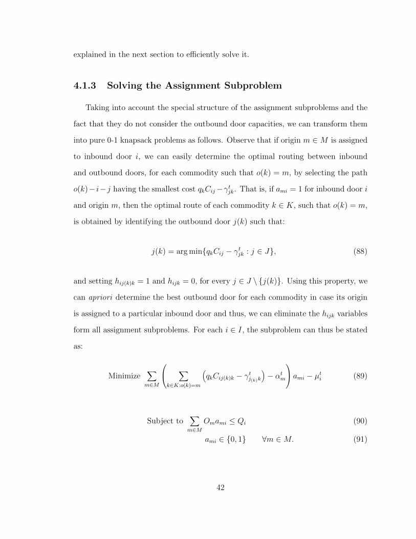
4.1.3 Solving the Assignment Subproblem

Taking into account the special structure of the assignment subproblems and the

fact that they do not consider the outbound door capacities, we can transform them

into pure 0-1 knapsack problems as follows. Observe that if origin m ∈M is assigned

to inbound door i, we can easily determine the optimal routing between inbound

and outbound doors, for each commodity such that o(k) = m, by selecting the path

o(k)− i−j having the smallest cost qkCij−γtjk. That is, if ami = 1 for inbound door i

and origin m, then the optimal route of each commodity k ∈ K, such that o(k) = m,

is obtained by identifying the outbound door j(k) such that:

j(k) = arg minqkCij − γtjk : j ∈ J, (88)

and setting hij(k)k = 1 and hijk = 0, for every j ∈ J \ j(k). Using this property, we

can apriori determine the best outbound door for each commodity in case its origin

is assigned to a particular inbound door and thus, we can eliminate the hijk variables

form all assignment subproblems. For each i ∈ I, the subproblem can thus be stated

as:

Minimize∑m∈M

∑k∈K:o(k)=m

(qkCij(k)k − γtj(k)k

)− αt

m

ami − µti (89)

Subject to∑m∈M

Omami ≤ Qi (90)

ami ∈ 0, 1 ∀m ∈M. (91)

42

This is a 0-1 knapsack problem which, although is known to be NP -hard, can be

efficiently solved in practice by suing the COMBO algorithm introduced in Martello

et al. [42].

4.1.4 Solving the Routing Subproblem

In Section 4.1.2 we provide a MIP formulation for the routing subproblem asso-

ciated with each outbound door j ∈ J and show that it corresponds to an ESPPRC.

This problem can be formally stated as follows. Let G = (V,A) be a graph where

A represents the set of arcs and V represents the set of vertices which contains the

set of customers C ⊂ V , a source vertex s and a destination vertex t. Let R be a

set of resources and for each arc (i, j) ∈ A, let Cij be the cost of the arc and W rij be

the consumption of the edge for the resource r ∈ R. For each pair of vertices i ∈ C

and resource r ∈ R, let ari and bri be two nonnegative values such that the total re-

source consumption along a path from s to i must belong to the interval [ari , bri ]. The

ESPPRC finds a minimum cost elementary path from source vertex s to destination

vertex t while satisfying all resource constraints.

Resource constraints vary on the type of considered problem. Thus, different re-

source constraints lead to different types of restrictions. Some of the most widely

used resource constraints include vehicle capacities where it is assumed that the vehi-

cles (or carriers) have known capacities and the capacities cannot be exceeded; time

windows where the customers have associated an earliest service time, a latest service

time and such that the vehicle should visit each customer within its given time in-

terval. Elementarity can also be regarded as a resource constraint. Indeed, once can

associate to each customer a binary resource initially set to false, and when a route

visits the customer, the resource is set to true. For a more general and traditional

43

approach to ESPPRC, we refer to Petersen et al. [43].

The DAVRP does not include time windows on the customers, but vehicle ca-

pacities are taken into account. The subproblem presented in Section 4.1.2 leads to

solving an ESPPRC for each outbound door j ∈ J where resources include only the

vehicle capacities, besides the obvious elementarily constraints. We label the out-

bound door as vertex ”0”, to represent both the source s and the destination t. The

customer set has an associated demand function d : C → Z and the vehicles have a

capacity of Q.

The ESPPRC is not only known to be NP -hard but also difficult to solve it to

optimality in practice. Baldacci et al. [44] presented a relaxation of the ESPPRC

called the ng-route relaxation. This relaxation aims at balancing the trade-off between

the CPU time and the quality of lower bounds obtained by relaxing the elementarity

of the paths, that is, by also considering some non-elementary paths. It has been

shown that this new relaxation provides strong lower bounds while greatly decreasing

the CPU times. For that reason, we use the ng-route relaxation in our implementation

of the solution to the routing subproblems to generate routes.

In what follows, the basic idea of ng-route relaxations and how it is implemented

efficiently is discussed following the notations of Baldacci et al. [44] and Pecin et

al. [45]. For each customer i ∈ C, let Ni ⊆ C be a subset of selected customers

which have a certain relationship with i. Most of the cases, the representation of

this relationship is a neighborhood criterion. For example, Ni contains the nearest

customers to i, including or excluding i depending on the case and the choice of the

user. Baldacci et al. [44] defines ng-sets Ni as including i and the nearest neighbors

of i. When a path P is being built, by the time it arrives at customer i, it has a set

Π(P ) representing the memory so far. If the customer i is already in the set Π(P ),

then the extension is forbidden and, similarly, if i does not belong to the set Π(P ),

44

the extension is allowed. At each extension, set Π(P ) is updated according to the set

Ni. Since every customer has different ng-sets, an update on Π(P ) will cause some

of the previously visited vertices to disappear from the set. Thus, those disappearing

customers could be visited in the future to form cycles. The size of each ng-set is

limited by a defined parameter |Ni| ≤ ∆(Ni). Note that if the ng-sets include all

customers, the problem simply becomes an ESPPRC. Similarly, if the ng-sets do not

contain any of the neighbors, then no elementarity is imposed and all of the cycles

are permitted. These implications lead to the discussion of the size of the ng-sets.

Obviously, including all the customers in ng-sets results in no relaxation; however,

the computational complexity for solving the problem greatly increases. On the other

hand, relaxing all the elementarily would result in bad lower bounds. Baldacci et al.

[44] discusses the choice of the parameter ∆(Ni) and state that the k-nearest neighbors

approach provides a good trade-off between quality of lower bounds and computation

time with k = 8 and 10.

Let P = (0, ip, ..., ip−1, ip) be a path starting at the depot, visiting a sequence

of customers and ending at customer ip. We define d(P ) =∑

i∈P Di as the total

demand serviced by path P and c(P ) as the total cost of path P . Let L (P ) =

(ip, d(P ),Π(P ), c(P )) be a label associated with a path P, which ends at customer ip.

d(P ) and Π(P ) are used to limit the feasible extensions of P , which can be extended

to a customer ip+1 if ip+1 /∈ Π(P ) and d(P ) +Dip+1 ≤ Q. After the extension occurs,

customer ip+1 becomes the last customer of the new path P ′ = (0...., ip, ip+1) and a

new label L (P ′) is obtained from the label L (P ) by following operation:

L (P ′) =(ip+1, d(P ) +Dip+1 ,Π(P ) ∩Nip+1 ∪ ip+1, c(P ) + cipip+1

). (92)

These labels are computed using a forward dynamic programming algorithm and,

45

in contrast to q-route relaxation, its complexity is no longer pseudo-polynomial. This

algorithm is exponential on the size of ∆(Ni), remaining pseudo-polynomial for fixed

∆(Ni). Its efficiency depends on the use of some techniques to speed up its execution.

In order to reduce the number of possible paths, a dominance rule is incorporated

into the algorithm. Given the labels of two paths L (P1) and L (P2), we say that

path P1 dominates path P2 if and only if every possible extension from P2 can be

done from P1 with a lower or equal total cost. Although this condition may be hard

to verify, it can be replaced by checking the following three conditions, which are

sufficient to guarantee correctness:

1. d(P1) ≤ d(P2),

2. c(P1) ≤ c(P2),

3. Π(P1) ⊆ Π(P2).

The dynamic programming algorithm starts by creating a matrix of size |N |(Q+1),

where each entry is a bucket B(d, i) containing labels that represent paths starting at

the depot and ending at customer i with a total capacity of d. In the beginning a single

label L0 = (0, 0, ∅, 0),∀i ∈ C are added to the first bucket and to a set of unexplored

labels U . Forward dynamic programming picks an unexplored label L from set U

and extends the label to all possible vertices, after which L is declared explored

and removed from U . The new labels created by extending an unexplored vertex

are added to set U and to the corresponding buckets (unless they are dominated by

existing labels). In the meantime, if a newly created label dominates an existing label,

such label is deleted from both buckets and set of unexplored vertices. A pseudocode

of the dynamic programming procedure is presented in Algorithm 1.

46

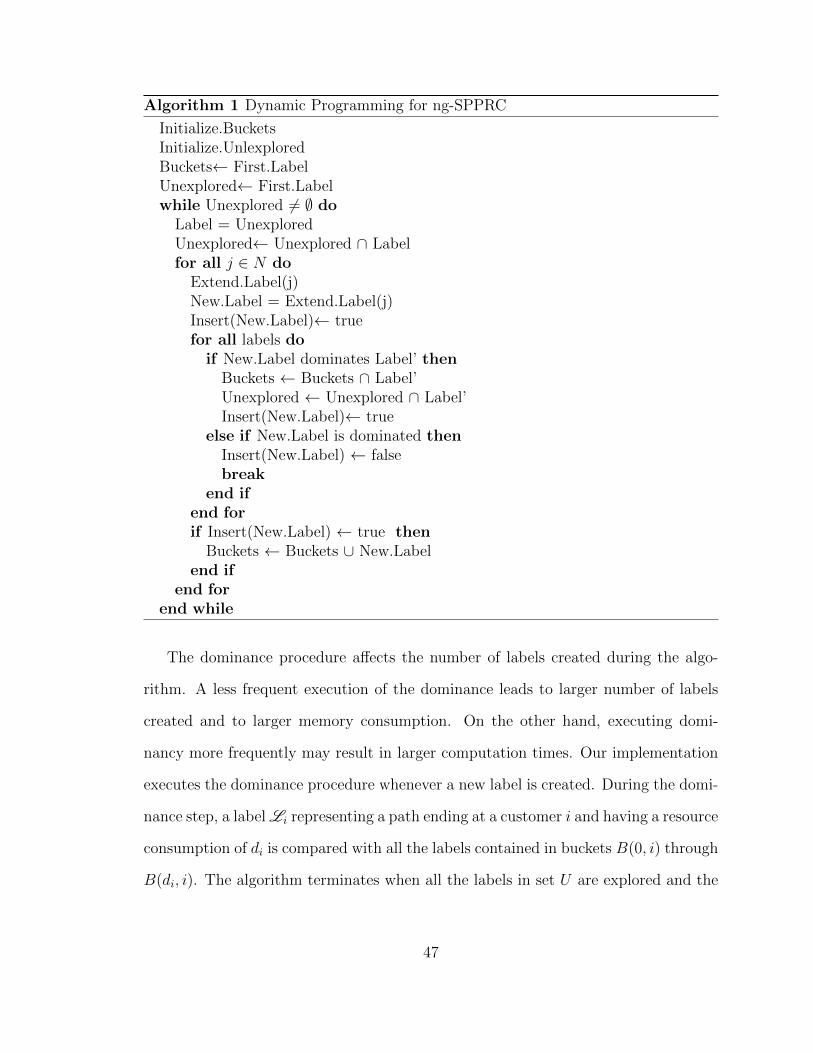
Algorithm 1 Dynamic Programming for ng-SPPRC

Initialize.BucketsInitialize.UnlexploredBuckets← First.LabelUnexplored← First.Labelwhile Unexplored 6= ∅ do

Label = UnexploredUnexplored← Unexplored ∩ Labelfor all j ∈ N do

Extend.Label(j)New.Label = Extend.Label(j)Insert(New.Label)← truefor all labels do

if New.Label dominates Label’ thenBuckets ← Buckets ∩ Label’Unexplored ← Unexplored ∩ Label’Insert(New.Label)← true

else if New.Label is dominated thenInsert(New.Label) ← falsebreak

end ifend forif Insert(New.Label) ← true then

Buckets ← Buckets ∪ New.Labelend if

end forend while

The dominance procedure affects the number of labels created during the algo-

rithm. A less frequent execution of the dominance leads to larger number of labels

created and to larger memory consumption. On the other hand, executing domi-

nancy more frequently may result in larger computation times. Our implementation

executes the dominance procedure whenever a new label is created. During the domi-

nance step, a label Li representing a path ending at a customer i and having a resource

consumption of di is compared with all the labels contained in buckets B(0, i) through

B(di, i). The algorithm terminates when all the labels in set U are explored and the

47

output of the algorithm is the least cost label of the buckets from B(1, 0) to B(Q, 0).

In other words, the least cost route that we are looking for our pricing problem will

be one of the labels ending at the depot vertex.

Note that the route created at the end of our pricing scheme may include cy-

cles, which means that the route is not elementary. Non-elementarity provides lower

bounds. One may enforce elementarity by the end of the pricing in many ways. Pecin

et al. [45] imposes elementarity by including all the customers in ng-sets, which

results in a non-cyclic route by the end of their dynamic programming algorithm.

However, we do not impose the routes to be elementary meaning that we accept the

final routes regardless of the cycles present in it. As a result, our implementation of

the CG algorithm will obtain a lower bound on the optimal solution of the MP.

4.1.5 Column Generation Algorithm

At the beginning of the CG algorithm, we start with an empty set of assignment

and routing columns. However, we add slack and artificial variables to ensure that at

every iteration we obtain a feasible solution to the RPM. At each iteration t of the

column generation, we solve the RMP with the set of existing columns ΩPit and ΩR

jt and

obtain new values for dual variables (αt, µt, γt, βt, πt). We then solve |I| assignment

subproblems and |J | routing subproblems to find columns with negative reduced cost

coefficients. If we find assignments and/or routes with negative reduced costs, we

add these new variables to the RMP and repeat the whole process for the iteration

t + 1 with updated set of columns ΩPi(t+1) and ΩR

j(t+1). Termination of the algorithm

occurs when both families of subproblems are not able to generate new variables with

negative reduced costs for any of the inbound/outbound doors.

Algorithm 2 depicts the pseudocode of our CG algorithm. By the end of the CG,

48

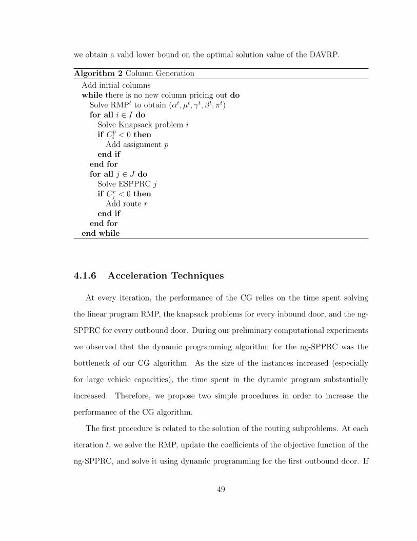
we obtain a valid lower bound on the optimal solution value of the DAVRP.

Algorithm 2 Column Generation

Add initial columnswhile there is no new column pricing out do

Solve RMPt to obtain (αt, µt, γt, βt, πt)for all i ∈ I do

Solve Knapsack problem iif Cp

i < 0 thenAdd assignment p

end ifend forfor all j ∈ J do

Solve ESPPRC jif Cr

j < 0 thenAdd route r

end ifend for

end while

4.1.6 Acceleration Techniques

At every iteration, the performance of the CG relies on the time spent solving

the linear program RMP, the knapsack problems for every inbound door, and the ng-

SPPRC for every outbound door. During our preliminary computational experiments

we observed that the dynamic programming algorithm for the ng-SPPRC was the

bottleneck of our CG algorithm. As the size of the instances increased (especially

for large vehicle capacities), the time spent in the dynamic program substantially

increased. Therefore, we propose two simple procedures in order to increase the

performance of the CG algorithm.

The first procedure is related to the solution of the routing subproblems. At each

iteration t, we solve the RMP, update the coefficients of the objective function of the

ng-SPPRC, and solve it using dynamic programming for the first outbound door. If

49

we are able to obtain a route with negative reduced for the first outbound door, we

add the route associated with the first outbound door to the RMP and we check if

this route would have a negative reduced cost for other outbound doors. If that is the

case, we add the same route to the RMP for each outbound door giving a negative

reduce cost and we do not longer solve their associated pricing problem. If we are

not able to add the route for a particular door, we solve its associated ng-SPPRC. By

following this simple procedure, we avoid potentially the solution of several routing

subproblems per iteration. It is worth mentioning that this can be seen as a heuristic

procedure for solving these problems, as the route with the minimum reduced cost

coefficient is not computed for each outbound door at every iteration.

Another approach to reduce the CPU time of CG is by adding a promising set

of initial columns to the RMP. This approach does not effect the performance of

the subproblems but greatly reduces the number of iterations needed to obtain the

optimal solution of the MP. The idea behind adding initial columns is that if we start

the algorithm with a subset of columns that are needed for the optimal basis then

the CG algorithm would skip many iterations to add these required columns.

We implement a simple local search (LS) heuristic in order to find initial columns

to the problem. We first start by creating an arbitrary feasible solution to the problem

and adding its associated columns assignment patterns and routes to the RMP. We

then apply a 2-exchange operation only on the routing part. This procedure allows

the exchange of two destination vertices regardless of which route they belong to. If

these two customers belong to different routes associated with the same outbound

door, then the assignment part still stays feasible and we add the associated two new

routes to the RMP. If the customers belongs to the same route, we only add a single

route to the RMP. If these two customers belong to different routes associated with

different outbound doors, we modify the assignment part of the problem. Fixing the

50

assignment part only requires one to change the outbound door assignment for the

commodities destined for these customers. In the end, we add the two new routes

and the assignments that have been changed to the RMP. This procedure continues

until we are not able to find better routes with the 2-exchange operator.

4.2 Heuristic Algorithms

In the previous section, we show how CG can be used to obtain lower bounds on

the optimal solution value of the DAVRP. However, the information generated during

the CG can also be employed to construct upper bounds for the DAVRP. We next

present two simple heuristic algorithms that use the sets of assignment patterns and

routes generated by CG to construct integer feasible solutions.

4.2.1 A Branch and Bound Based Heuristic

Once the LP relaxation of the set partitioning formulation has been optimally

solved by CG at iteration t, we can impose integrality constraints on the current sets

ΩPit , i ∈ I and ΩR

jt, j ∈ J , and solve the resulting integer restricted master problem.

We use a standard branch and bound (BB) algorithm in which the columns are only

generated at the root node when solving the linear MP, and no columns are generated

at all in the rest of the nodes of the enumeration tree. Since we only have a small

subset of all the possible variables, this integer program can be easily solved using a

general purpose solver (such as CPLEX).

4.2.2 A Local Search Heuristic

The second heuristic is a simple local search (LS) algorithm which is applied to

improve the initial solution obtained from the BB heuristic. In our LS, we implement

51

four different neighborhoods. The first two manipulate the assignment of origins to

inbound doors whereas the last two neighborhoods modify the routes from outbound

door to destinations.

The first neighborhood is a shift neighborhood which considers the reassignment

of a single origin from a currently assigned inbound door to another, while respecting

the capacity constraints. Consider an origin point m assigned to an inbound door i.

We temporary assign m to a different inbound door i′ such that this new assignment

will remain feasible for the capacity of inbound door i′. Then, we change the inbound

door assignment of all the commodities originating at m from i to i′. For each m ∈M ,

we explore all the possible (i, i′) ∈ I× I pairs and perform a move if the best solution

improves the incumbent.

The second neighborhood is a swap neighborhood which considers the reassign-

ment of two origins by interchanging their inbound doors. Consider two origin points

m and m′ assigned to the inbound doors i and i′, respectively, such that i 6= i′. We

reassign m to i′ and m′ to i, if the capacities for inbound doors i and i′ are not

violated by these reassignments. As a consequence, we also change the inbound door

assignments of all the commodities originated at m to i′ and all the commodities

originated at m′ to i. We explore all the feasible pairs (m,m′) ∈M ×M and perform

a move if the best solution improves the incumbent.

The third neighborhood performs modifications to the routing part of the solution.

It consists of removing a customer from a route and inserting it to another route. If

these two routes belong to the same outbound door, the routing inside the cross-dock

needs no changes. Consider a route r associated with an outbound door j that travels

from a destination point n1 to n and then from n to n2. We remove the vertex n

from route r and insert it to another route r′ associated with an outbound door j′, in

between customer n′1 and n′2, such that r 6= r′, and the insertion does not violate the

52

vehicle capacity of route r′ as well as the capacity of outbound door j′. If j = j′, the

routing between inbound and outbound doors does not change. However, if j 6= j′

then the change on the inner routing part is such that commodities destined for

vertex n are changed from outbound door j to j′. We explore all feasible reinsertions

of destinations n ∈ N to every position of the set of existing routes, and perform a

move if the best solution improves the incumbent.

The fourth neighborhood considers swapping two destination vertices regardless

of the routes they belong to. Let n and n′ be two destination points belonging to

routes r and r′ associated with outbound doors j and j′, respectively. Let n1 be the

preceding customer and n2 be the successor of n on route r. Similarly, let n′1 and n′2

be the predecessor and successor of vertex n′ on route r′. We exchange the vertices n

and n′ such that the resulting routes r and r′ do not exceed the vehicle capacities and

the outbound doors j and j′ do not exceed the outbound door capacities. If j = j′,

the routing between inbound and outbound doors does not change. However, in the

case of routes r and r′ belonging to different outbound doors, the outbound door

assignments for commodities that are destined for vertex n are changed from j to j′

and similarly for the commodities destined for n′ are changed from outbound door

j′ to j. We explore all the feasible pair of exchanges (n, n′) ∈ N ×N and perform a

move if the best solution improves the incumbent.

Our implementation of the LS performs a sequential search on these four neigh-

borhoods, starting from the first one. If a neighborhood is unable to improve the

incumbent solution, LS jumps to the next neighborhood. Otherwise, it keeps search-

ing on the same one. If a neighborhood is unable to improve the solution, LS jumps

to the next neighborhood. The algorithm stops when all the neighborhoods fails to

improve the incumbent solution and thus, a local optimal solution is reached.

53

5 Computational Results

A computational study was conducted in order to test the performances of the

MIP models and the solution methodology introduced in the previous chapters. In

the first part of the computational experiments, we focus on a comparison of three

MIP formulations (F2, F3 and F4) presented in Chapter 3. Given that the natural

three index formulation requires an ad-hoc branch-and-cut algorithm to handle the

exponential number of rounded capacity constraints, we have decided not to include

it in our computational results. In the second part, we analyze the performance

of the column generation algorithm and compare it with the most promising of the

three MIP formulations. In the last part, we show the performance of the heuristic

algorithm presented in Section 4.2.

The MIP formulations and the column generation algorithm were coded in C using

the callable library of CPLEX 12.5.1. All the experiments were implemented and run

on Windows OS with an Intel Core i7 processor at 2.40 GHz and 8GB of RAM. A

maximum time limit of two hours was used in all experiments.

We have performed the computational experiments using randomly generated in-

stances. We generated instances with |N | = 7, 10, 15, 20, 25, |M | = 5, 7, 10, 15

and |I| = 2, 3, 4, 5, 6 such that |M | ≤ |N |, |I| = |J | ≤ |M | and |N | = |K|. For each

value of n ∈ N we randomly generated the (x, y)-coordinates of the vertices from

a continuous uniform distribution in [0, 150] × [0, 150] and define the traveling cost

between pairs of vertices as the Euclidian distance. For each inbound-outbound door

pair (i, j) ∈ I × J we generated the unit material handling cost as Cij ∼ [0, 20]. For

each n ∈ N we generated commodity quantities as qn ∼ [0, 20] and originate these

54

commodities randomly at the origin points such that the number of commodities

originating at an origin point is at most equal to 3. For each inbound and outbound

door, we randomly select capacities from the set Qi, Qj ∈ 40, 50, 60, 70, 80, 100, 150.

Finally, we consider two different values for fixed cost of operating a vehicle H ∈

100, 150 and six different values for vehicle capacities Q ∈ 20, 30, 40, 50, 60, 70 for

each instance.

Preliminary experiments showed that some of the instances were easy to solve.

These instances were omitted from the computational experiments. The remaining

results with a total of 75 instances.

5.1 A Comparison of MIP Formulations

In this section, we compare the LP bounds and the best upper bounds obtained

by F2, F3 and F4 when solved by CPLEX. Computational results are summarized in

Table 3.

The first two columns contain the number of origin vertices |M | and the number

of destination vertices |N |, respectively. The next three columns correspond to the

percent deviation between the optimal solution value and LP bounds, the percent

deviation between the optimal solution value and the best upper bounds, and the CPU

time in seconds needed to obtain an optimal solution with F2, F3 and F3, respectively.

The LP relaxation gap is computed as LP = 100× (OPT −LBF )/OPT , where OPT

is the optimal solution value and LBF is the lower bound obtained with F1, F2 and

F3, respectively. When the optimal solution value cannot be found within the given

time limit, LP relaxation gap is computed as LP = 100 × (UBbest − LBF )/UBbest,

where LBF are the lower bound obtained with F1, F2 and F3, respectively, and

UBbest is the best upper bound obtained. Upper bound gap is computed as UB =

55

Table 3: Comparison of MIP formulations.

F2 F3 F4

|M | |N | LP UB CPU LP UB CPU LP UB CPU

5 7 14.22 0.00 3.12 14.46 0.00 2.18 49.85 0.00 3.2613.80 0.00 3.28 13.72 0.00 2.00 43.84 0.00 15.088.07 0.00 2.05 8.50 0.00 3.44 34.35 0.00 10.0613.12 0.00 3.08 13.90 0.00 3.81 34.23 0.00 17.14

5 10 10.29 0.00 26.87 9.82 0.00 7.92 66.86 0.00 762.0013.90 0.00 4.30 13.90 0.00 2.62 59.64 0.00 time6.76 0.00 4.50 6.98 0.00 2.32 49.69 0.00 time10.89 0.00 114.23 10.73 0.00 5.87 39.43 0.00 0.7513.29 0.00 8.00 13.49 0.00 5.00 34.81 0.00 0.989.70 0.00 60.34 8.93 0.00 32.84 49.40 0.00 15.0011.33 0.00 17.04 11.09 0.00 25.51 41.30 0.00 time6.05 0.00 15.18 5.71 0.00 17.35 32.23 0.00 1.179.76 0.00 6.08 9.58 0.00 5.96 32.21 11.29 time15.70 0.00 90.29 12.11 0.00 13.58 47.23 0.00 time6.34 0.00 45.89 5.06 0.00 9.90 30.81 0.00 1.5812.66 0.00 28.00 9.26 0.00 10.31 41.39 0.00 0.639.82 0.00 24.00 7.70 0.00 9.67 34.10 0.00 0.5010.98 0.00 65.00 10.02 0.00 24.13 31.41 0.00 0.3314.82 0.00 27.22 14.30 0.00 9.41 42.18 0.00 0.0812.21 0.00 6.35 12.46 0.00 3.12 32.92 0.00 0.03

7 10 6.12 0.00 3480.00 5.46 0.00 1442.56 25.52 0.00 600.002.96 0.00 74.00 2.67 0.00 26.32 18.62 0.00 time5.07 0.00 18.45 4.88 0.00 1301.87 17.64 0.00 time

10 10 6.38 0.00 30.30 5.82 0.00 277.45 64.70 0.00 11.502.29 0.00 35.90 1.81 0.00 9.05 57.76 0.00 time10.76 0.00 5.60 10.58 0.00 6.68 57.35 0.00 time14.06 0.00 7.00 12.14 0.00 8.95 42.69 0.00 2.6019.27 0.00 10.00 15.37 0.00 9.85 43.39 0.00 7.7015.67 0.00 25.00 12.51 0.00 9.10 35.73 0.00 160.8015.71 0.00 254.22 13.89 0.00 90.00 32.43 0.00 423.809.12 0.00 4.00 8.22 0.00 5.92 25.02 0.00 98.005.72 0.00 21.80 7.79 0.00 10.63 58.67 0.00 1.607.51 0.00 447.00 7.77 0.00 60.53 61.10 0.00 223.004.25 0.00 26.20 3.81 0.00 9.59 54.13 0.00 time10.90 0.00 9.30 10.83 0.00 5.23 53.25 0.00 time7.76 0.00 11.70 8.82 0.00 7.33 50.90 0.00 2.0015.41 0.00 206.80 13.79 0.00 10.65 60.97 0.00 120.0014.20 0.00 66.70 12.50 0.00 8.96 54.76 0.00 time8.59 0.00 40.80 7.10 0.00 114.00 47.14 0.00 time14.54 0.00 100.50 13.35 0.00 6.31 47.01 0.00 time

56

Table 3: Continued.

F2 F3 F4

|M | |N | LP UB CPU LP UB CPU LP UB CPU

10 10 7.58 0.00 11.00 8.28 0.00 7.10 56.51 0.00 3.4015.15 0.00 33.03 14.10 0.00 17.08 66.70 0.00 231.0013.72 0.00 34.00 12.59 0.00 7.52 60.95 0.20 time7.91 0.00 36.00 6.91 0.00 40.37 53.82 0.60 time14.89 0.00 26.00 14.10 0.00 8.92 53.82 0.27 time

10 15 12.92 0.00 113.50 10.66 0.00 26.93 30.03 0.00 3.9013.28 0.85 time 10.79 0.00 1687.51 31.19 0.15 time7.81 7.42 time 5.88 0.00 36.55 22.57 0.77 time7.99 2.63 time 6.92 0.00 22.24 20.17 0.38 time5.73 0.29 time 4.99 0.00 80.74 16.42 0.00 time

15 15 5.50 0.00 time 5.67 0.00 3915.50 28.62 0.00 9.606.07 0.00 452.50 5.27 0.00 13.35 33.52 0.00 time3.42 0.00 526.50 2.60 0.00 245.52 27.20 0.27 time6.35 0.16 time 5.79 0.00 85.41 26.22 0.38 time4.20 0.44 time 3.83 0.00 15.21 22.04 0.66 time8.16 0.00 39.00 8.32 0.00 7000.00 50.23 0.00 95.809.83 0.00 253.00 8.94 0.00 25.47 61.96 0.00 time4.60 0.13 time 3.60 0.00 6954.00 54.45 0.29 time11.74 4.25 time 11.06 0.00 70.89 53.70 0.67 time7.88 2.64 time 7.40 0.00 15.28 48.05 0.07 time

10 20 10.32 9.58 time 9.59 0.00 time 69.74 1.03 time6.25 21.97 time 5.66 0.00 time 63.39 0.86 time12.03 5.20 time 11.28 0.00 time 61.69 2.09 time10.76 0.00 time 10.10 0.00 390.00 56.67 0.66 time19.71 24.27 time 16.88 0.00 time 43.46 0.13 time14.38 5.63 time 11.10 0.00 time 33.91 2.27 time13.50 9.45 time 11.40 0.00 time 29.77 2.65 time

15 25 7.84 0.04 time 8.63 0.00 time 53.54 0.79 time11.45 5.08 time 10.51 0.00 time 63.08 5.74 time10.37 23.38 time 8.82 0.00 time 56.87 1.84 time15.34 9.71 time 14.10 0.00 time 55.05 3.64 time7.30 0.75 time 7.82 0.00 time 58.96 1.14 time10.27 0.00 time 9.66 0.00 time 67.48 0.15 time8.71 8.67 time 7.68 0.00 time 61.59 0.92 time10.85 9.42 time 9.99 0.00 time 58.27 2.69 time

Average 10.18 2.03 9.36 0.00 45.18 1.02

57

100× (UBbest−UBF )/UBbest, where UBF are the upper bounds obtained by F1, F2

and F3, respectively. Whenever CPLEX is not able to solve an instance within the

time limit, we write time in the corresponding entry of the table.

During the computational experiments, we observed that the CPU times needed to

solve the LP relaxations never exceeded ten seconds. Therefore CPU times associated

with LP relaxations were omitted from the table.

Table 3 shows that the best formulation is the F3 in terms of number of instances

solved to optimality in the given time limit. F3 formulation is able to obtain the

optimal solution for all the instances with less than 20 vertices. On the other hand,

none of the formulations are able to obtain optimal solution for instances with 20 and

more vertices in the given time limit except one single instance. We can also observe

that F2 is able to obtain the optimal solution for most of the instances in the given

time limit. F4 turns out to be the worst formulation in terms of obtaining optimal

solutions as it is not able to solve 44 instances to optimality in the given time limit.

F4 formulation proves to be the worst in terms of LP relaxation gaps with an

average of 45.2% deviation. Overall, F2 and F3 show similar LP relaxation gaps. F2

was able to obtain smaller LP relaxation gaps for 14 instances whereas F3 obtained

smaller gaps for the rest of the instances. F2 and F3 show an average of 10.2% and

9.4% LP relaxation gaps, respectively. F3 obtained the best upper bounds for all the

instances that were not solved to optimality. For the remaining instances, F4 obtained

better upper bounds than F2. For the instances that were solved to optimality with

all of the formulations, F2, F3 and F4 showed variation in terms of CPU times.

Overall, the multi commodity flow formulation (F3) outperforms F2 and F4 in

terms of number of instances solved to optimality, LP relaxation gaps and the best

upper bounds found.

58

5.2 Column Generation

In this section we compare the LP relaxation bounds obtained by the column

generation with the ones obtained by F3. We also look at the changes in the perfor-

mance of column generation when the heuristic pricing technique (Section 4.1.6) is

used. Computational results are summarized in Table 4.

The first two columns contain the number of origin and destination points, re-

spectively. The following four columns provide the CPU times in seconds and num-

ber of iterations (NI) needed to solve the LP relaxation with pure column gener-

ation (CG) and column generation with heuristic pricing technique (ICG), respec-

tively. The seventh column give the percent reduction in CPU times when heuristic

pricing technique is incorporated. The reduction is computed as Acceleration =

100 × (CPUICG/CPUCG), where CPUCG is the time spent by pure column genera-

tion and CPUICG is the CPU time of column generation with heuristic pricing tech-

nique. The last two columns provide the percent deviation between the upper bound

obtained by F3 and LP relaxation bounds obtained by column generation and F3,

respectively. LP relaxation gaps are calculate as LP = 100× (UBF3 − LPF )/UBF3,

where UBF3 is the upper bound obtained by F3 and LPF is the LP relaxation bound

obtained by column generation and F3, respectively.

Table 4 shows that column generation always obtained better LP relaxation bounds

than F3. We mentioned in the previous section that F2 was able to obtain better LP

relaxation bounds than F3 for 14 instances. Column generation also provided better

LP relaxation bounds than F2 for these instances. However, it was observed that for

instances with large vehicle capacities column generation showed lager LP relaxation

gaps. These results can be partially explained by the fact that column generation

uses ng-Route relaxation to approximate the ESPPRC. It was also observed that

59

Table 4: Performance of column generation.

CG ICG CG F3

|M | |N | CPU NI CPU NI Acceleration LP LP

5 7 1.40 10 1.40 10 100.00 5.23 14.462.18 14 1.62 15 74.31 8.53 13.725.80 17 2.70 17 46.55 4.16 8.5015.40 18 7.00 19 45.45 10.77 13.90

5 10 2.70 24 1.55 24 57.41 7.67 9.8238.00 29 27.50 30 72.37 12.42 13.90351.00 33 135.20 34 38.52 5.73 6.985.50 28 3.91 28 71.09 8.42 10.7353.00 31 67.90 37 128.11 10.84 13.494.00 21 1.70 22 42.50 5.34 8.9354.70 23 26.80 23 48.99 9.11 11.0912.50 27 9.20 27 73.60 4.10 5.7160.00 29 30.90 29 51.50 8.40 9.585.00 16 3.00 17 60.00 7.72 12.11

302.00 25 94.80 28 31.39 1.74 5.063.70 22 2.20 22 59.46 6.43 9.2659.00 30 25.50 30 43.22 5.07 7.70234.00 32 117.50 32 50.21 7.19 10.024.00 21 2.50 21 62.50 9.51 14.3095.70 27 36.70 30 38.35 9.44 12.46

7 10 5.00 16 2.43 17 48.60 1.27 5.4612.00 25 7.81 26 65.08 0.48 2.67108.00 29 65.40 29 60.56 2.71 4.88

10 10 1.70 15 1.50 15 88.24 0.00 5.823.60 15 2.50 15 69.44 0.00 1.8120.70 24 13.10 24 63.29 8.86 10.581.30 14 0.90 14 69.23 1.36 12.141.60 14 1.50 14 93.75 1.93 15.372.90 20 2.50 20 86.21 3.47 12.5113.50 28 9.10 30 67.41 8.62 13.8961.00 32 38.80 33 63.61 3.73 8.221.30 11 1.50 11 115.38 0.00 7.792.80 19 2.40 19 85.71 0.20 7.7717.70 24 10.50 24 59.32 0.00 3.8183.00 28 26.30 28 31.69 7.34 10.831.80 13 1.10 14 61.11 3.72 8.821.60 13 2.10 17 131.25 4.04 13.793.50 17 2.50 18 71.43 7.27 12.5014.60 25 7.20 25 49.32 2.19 7.1064.70 31 26.50 31 40.96 9.31 13.35

60

Table 4: Continued.

CG ICG CG F3

|M | |N | CPU NI CPU NI Acceleration LP LP

10 10 1.70 9 1.10 11 64.71 4.94 8.281.60 11 2.00 12 125.00 5.75 14.104.20 22 2.80 22 66.67 8.94 12.5914.00 18 8.40 18 60.00 3.62 6.9193.80 26 30.40 26 32.41 11.40 14.10

10 15 3.60 18 1.70 18 47.22 0.79 10.665.00 27 3.50 27 70.00 1.75 10.7918.00 30 11.70 30 65.00 0.15 5.8893.00 39 72.30 42 77.74 3.63 6.92308.60 55 173.30 57 56.16 2.57 4.99

15 15 5.20 20 2.10 20 40.38 1.67 5.677.30 26 3.70 26 50.68 2.89 5.2726.60 36 11.80 36 44.36 0.30 2.6092.50 39 73.80 39 79.78 3.60 5.79461.00 57 206.20 57 44.73 2.24 3.835.20 19 1.80 20 34.62 3.68 8.326.50 27 3.80 27 58.46 6.27 8.9423.00 37 12.10 37 52.61 0.79 3.60127.00 42 89.80 41 70.71 8.38 11.06456.00 53 229.60 50 50.35 5.34 7.40

10 20 65.00 42 23.80 43 36.62 5.66 9.59525.00 51 141.00 50 26.86 3.54 5.66262.00 50 264.00 50 100.76 7.61 11.281514.00 64 482.40 64 31.86 7.03 10.1019.00 42 15.90 42 83.68 5.80 16.88145.00 48 59.50 49 41.03 4.35 11.10646.00 69 314.00 72 48.61 6.59 11.40

15 25 19.00 45 27.10 52 142.63 2.63 8.63145.00 62 71.90 62 49.59 5.80 10.511198.00 79 293.20 80 24.47 5.00 8.822206.00 97 734.20 99 33.28 11.43 14.10

15 25 21.00 42 14.30 45 68.10 3.65 7.82111.00 63 54.00 67 48.65 6.57 9.66861.00 72 342.60 72 39.79 5.15 7.682237.00 85 888.60 85 39.72 8.17 9.99

Average 179.46 32.16 73.25 32.89 61.66 5.09 9.36

61

CPU times of CG increased dramatically as the vehicle capacities increased. These

results are due to the fact that it takes longer times to solve the dynamic programming

algorithm for ESPPRC with large vehicle capacities.

Overall, ICG showed smaller CPU times compared to CG. On the other hand,

number of iterations either stayed the same or increased slightly. ICG adds different

columns compared to pure column generation at each iteration. By this reason, ICG

ends up spending more iterations. For six instances, ICG spent more time than

CG due to the increased number of iterations. For the rest of the instances, the

heuristic pricing technique was observed to decrease the CPU times. Especially for

the instances with large vehicle capacities, the CPU times decreased dramatically.

We mentioned in Section 5.1 that the CPU time spent by F3 to solve the LP

relaxation never exceeded 10 seconds for any instance. We omitted these results from

the tables but it is worth the mention that the CPU times of ICG are reasonably

small enough to be compared with the CPU times of F3 for small scale instances.

5.3 Heuristic Approaches

In Chapter 4, we proposed 2 different methods to obtain upper bounds. Both

of these methods are based on solving the restricted master problem with CPLEX

by imposing integrality on the existing variables. Additionally, the second approach

applies a local search heuristic to the final integer solution obtained by CPLEX. In

this section, we present three sets of integer results obtained by column generation

algorithm. The first set of results does not include adding columns in the beginning

of the column generation. The second set corresponds to the results obtained when

initial columns are added. Finally, the last set of results is when initial columns are

added and the local search heuristic is applied to the final integer solution. All three

62

sets of results incorporate the heuristic pricing technique.

During the computational experiments, it was observed that relaxing the set par-

titioning constraints (60) for assignments to (98) gave more flexibility to the integer

solutions obtained by CPLEX in the end of column generation algorithm. At the

same time, relaxing these constraints did not cause any changes on the LP relaxation

bounds obtained. Thus, we performed the experiments to obtain integer feasible

solutions with the following set of constraints (98), instead of (60):

∑m∈M

∑p∈ΩP

i

Omapmi ≤ Qi ∀i ∈ I. (93)

The corresponding results are given in Table 5. The first two columns denote the

number of origin and destination vertices, respectively. The next two columns branch

and bound based heuristic (BBH) provide the CPU time in seconds to solve the column

generation plus the resulting integer program, and the percent deviation between the

upper bounds obtained by column generation and F3. Similarly, columns 5 and 6 give

the CPU time in seconds to solve the column generation with initial columns (IC) plus

the resulting integer program, and the gap in percentage between the upper bounds

obtained by column generation with initial columns and F3. The last column provides

the gaps between F3 and the upper bounds obtained with applying local search (LS)

by the end of column generation with initial columns. All the upper bound gaps in

Table 5 are computed as UB = 100 × (UBF3 − UBF )/UBF3, where UBF3 is the

best upper bound obtained by F3 and UBF is the upper bound obtained by column

generation, column generation with initial columns, and heuristic, respectively.

Comparing the CPU times of BBH in Table 5 with the ICG in Table 4 reveals

the fact that CPLEX takes less than a second to solve the integer master problem.

Adding initial columns decreases the CPU time of column generation; however, in

63

Table 5: Performance of heuristic.

BBH BBH+IC BBH+IC+LS

|M | |N | CPU UB CPU UB UB

5 7 1.52 0.00 1.42 0.00 0.001.64 2.88 1.92 0.00 0.002.73 25.61 3.38 20.54 1.627.03 13.65 7.76 13.65 2.21

5 10 1.56 21.28 2.86 0.50 0.5027.59 19.58 26.83 4.75 3.23135.30 67.37 130.18 50.50 1.244.00 10.92 2.30 0.00 0.0067.94 - 73.68 30.04 10.751.79 12.84 3.43 2.45 2.4526.91 12.74 21.93 5.03 2.479.29 29.56 6.57 24.19 1.9630.95 24.31 23.54 13.02 0.003.06 17.85 3.14 8.89 0.4494.93 55.78 89.05 55.78 14.212.23 10.95 2.64 8.27 2.4025.55 9.21 24.23 0.91 0.91117.54 46.40 84.66 32.20 3.922.55 13.20 2.14 6.89 0.0036.75 31.31 40.11 10.23 0.65

7 10 2.55 9.42 4.85 6.23 4.157.89 13.47 8.61 12.90 2.2965.49 14.61 60.34 7.63 2.73

10 10 1.56 0.00 1.36 0.00 0.002.55 0.00 2.18 0.00 0.0013.15 16.15 13.94 0.59 0.591.00 3.04 1.15 1.11 1.111.57 0.00 1.47 0.00 0.002.56 1.40 2.16 1.40 1.409.13 7.73 4.93 5.22 0.0038.82 11.07 31.25 0.58 0.581.58 0.00 1.32 0.00 0.002.45 13.24 2.56 2.23 2.2310.55 0.00 7.32 0.00 0.0026.35 16.00 20.65 1.38 1.381.18 0.00 1.48 0.00 0.002.16 0.00 1.47 0.00 0.002.55 0.00 2.36 0.00 0.007.25 14.81 5.45 1.42 1.4226.55 13.56 24.25 1.76 0.10

64

Table 5: Continued.

BBH BBH+IC BBH+IC+LS

|M | |N | CPU UB CPU UB UB

10 10 1.18 3.24 1.18 3.24 1.852.06 3.47 1.37 3.47 1.882.86 4.56 2.96 4.56 3.268.46 19.53 6.56 19.53 6.4130.46 18.66 27.92 18.35 3.68

10 15 1.84 0.26 2.00 0.26 0.263.59 0.57 4.28 0.57 0.5711.76 7.37 8.20 5.32 3.3872.37 3.70 49.95 0.23 0.23173.36 2.97 164.25 0.29 0.29

15 15 2.20 0.10 4.65 0.10 0.103.79 0.27 5.77 0.00 0.0011.90 5.35 13.05 5.35 0.5673.85 1.49 50.05 0.82 0.82206.24 5.13 200.65 0.00 0.001.92 0.68 2.45 0.11 0.113.91 0.30 3.37 0.00 0.0012.18 16.99 9.57 9.35 0.8889.91 11.19 32.27 1.01 1.01229.67 10.62 139.63 0.04 0.04

10 20 24.01 12.40 47.40 10.57 1.89141.26 30.94 122.13 21.04 1.62264.07 23.58 134.95 14.31 7.04482.46 31.96 518.82 22.94 2.4115.96 3.48 11.04 0.64 -1.0959.57 24.49 33.26 10.14 3.76314.27 29.36 197.76 20.24 5.48

15 25 27.30 3.95 33.60 3.95 0.0772.15 10.59 53.70 4.73 1.98293.40 22.03 191.40 -3.05 -3.05736.48 30.10 720.56 20.58 1.6314.55 10.05 31.60 6.63 1.8254.27 24.24 49.07 15.24 3.23342.79 30.70 377.09 30.03 0.71888.86 47.95 781.86 34.80 8.36

Average 73.37 13.68 63.80 8.21 1.71

65

some cases the CPU time has increased. This result can be explained by the same

effect (increase in the number of iterations) that was explained in Section 5.2. We

also observed that the local search heuristic never spent more than a second and thus,

we omitted these results from the table.

Table 5 shows that adding initial columns not only affects the CPU times but also

the quality of the upper bounds. Adding initial columns improved the upper bounds

in most cases. Local search was able to improve the final solution for 41 instances.

Moreover, column generation was able to obtain better upper bounds than F3 in two

instances. Furthermore, column generation was able to solve fourteen instances to

optimality within less CPU time than. Overall, adding initial columns and applying

local search on the final solution yields the best results with an average upper bound

gap of 1.71%.

66

6 Conclusion and Future Research

In this thesis we have introduced the Dock-Door Assignment and Vehicle Routing

Problem (DAVRP). It is a combinatorial optimization problem combining dock-door

assignment and vehicle routing decisions in a cross-docking context. To the best of

authors’ knowledge, this problem has not been previously studied in the literature. We

presented five different mixed integer programming formulations for the DAVRP. We

also developed a column generation algorithm based on a set partitioning formulation

and a local search heuristic.

We have provided a computational study of the different MIP formulations us-

ing CPLEX. The multi commodity flow based formulation outperformed the other

formulations when solved with a general purpose solver. We observed that none of

the formulations was able to prove optimality for instances with more than 20 des-

tination vertices in the given time limit. Furthermore, we compared the results of

the proposed column generation methodology with the multi commodity flow based

formulation. Our solution algorithm always obtained better LP bounds. In addition,

the local search heuristic was able to find feasible solutions in reasonable CPU times.

There are several directions of future research. First of all, developing additional

heuristic strategies for the pricing scheme would improve the performance of the

column generation. Also, defining larger neighborhood structures for the final heuris-

tic would lead to improvements on the obtained upper bounds. Another important

research avenue would be to embed the column generation procedure into an enumer-

ation tree to obtain optimal solutions to the DAVRP.

67

7 Bibliography

[1] J. V. Belle, P. Valckenaers, and D. Cattrysse, “Cross-docking: State of the art,”

Omega, vol. 40, no. 6, pp. 827–846, 2012.

[2] E. Kinnear, “Is there any magic in cross-docking?,” Supply Chain Management,

vol. 2, no. 2, pp. 49–52, 1997.

[3] U. M. Apte and S. Viswanathan, “Effective cross docking for improving distri-

bution efficiencies,” International Journal of Logistics, vol. 3, no. 3, pp. 291–302,

2000.

[4] M. Hammer, “Deep change: How operational innovation can transform your

company,” Harvard Business Reveal, vol. 82, no. 4, pp. 84–93, 2004.

[5] D. Agustina, C. Lee, and R. Piplani, “A review: Mathematical models for cross

docking planning,” International Journal of Engineering Business Management,

vol. 2, no. 2, pp. 47–54, 2010.

[6] R. Musa, J.-P. Arnaout, and H. Jung, “Ant colony optimization algorithm to

solve the transportation problem of cross-docking network,” Computers & In-

dustrial Engineering, vol. 59, no. 1, pp. 85–92, 2010.

[7] H. Charkhgard and A. Y. Tabar, “Transportation problem of cross-docking net-

work with three-dimensional trucks,” African Journal of Business Management,

vol. 5, no. 22, pp. 9297–9303, 2011.

68

[8] S. Sung and S. H. Song, “Integrated service network design for a cross-docking

supply chain network,” The Journal of the Operational Research Society, vol. 54,

no. 12, pp. 1283–1295, 2003.

[9] Z. Miao, F. Yang, K. Fu, and D. Xu, “Transshipment service through crossdocks

with both soft and hard time wimdows,” Annals of Operations Research, vol. 192,

no. 1, pp. 21–47, 2012.

[10] A. Lim, Z. Miao, B. Rodrigues, and Z. Xu, “Transshipment through crossdocks

with inventory and time windows,” Naval Research Logistics, vol. 52, no. 8,

pp. 724–733, 2005.

[11] L. Yeung and C. Lee, Decision Engineering, ch. 1, pp. 1–22. Springer London,

2012.

[12] W. Yu and P. J. Egbelu, “Scheduling of inbound and outbound trucks in cross

docking systems with temporary storage,” European Journal of Operational Re-

search, vol. 184, no. 1, pp. 377–396, 2008.

[13] N. Boysen, “Truck scheduling at zero-inventory cross docking terminals,” Com-

puters & Operations Research, vol. 37, no. 1, pp. 32–41, 2010.

[14] L. Y. Tsui and C.-H. Chang, “A microcomputer based decision support tool

for assigning dock doors in freight yards,” Computers & Industrial Engineering,

vol. 19, no. 1-4, pp. 309–312, 1990.

[15] L. Y. Tsui and C.-H. Chang, “An optimal solution to a dock door assignment

problem,” Computers & Industrial Engineering, vol. 23, no. 1-4, pp. 283–286,

1992.

69

[16] M. Guignard, P. M. Hahn, A. A. Pessoa, and D. C. da Silva, “Algorithms for

the cross-dock door assignment problem,” in Fourth International Workshop on

Model-Based Metaheuristics, 2012.

[17] Y. L. Yi-Rong Zhu, Peter M. Hahn and M. Guignard-Spielberg, “New approach

for the cross-dock door assignment problem,” in Pesquisa Operacional na Gestao

do Conhecimento, 2009.

[18] V. Yu, D. Sharma, and K. G. Murty, “Door allocations to origins and destinations

at less-than-truckload,” Journal of Industrial & Systems Engineering, vol. 2,

no. 1, pp. 1–15, 2008.

[19] R. Bermudez and M. H. Cole, “A genetic algorithm approach to door assign-

ments in breakbulk terminals,” tech. rep., Mack-Blackwell Rural Transportation

Center, University of Arkansas, 2011.

[20] A. M. Brown, “Improving the efficiency of hub operations in a less-than-truck-

load distribution network,” Master’s thesis, Virginia Polytechnic Institute &

State University, 2003.

[21] Y. A. Bozer and H. J. Carlo, “Optimizing inbound and outbound door assign-

ments in less-than-truckload cross-docks,” IIE Transactions, vol. 40, no. 11,

pp. 1007–1018, 2008.

[22] Y. Oh, H. Hwang, C. N. Cha, and S. Lee, “A dock-door assignment problem

for the korean mail distribution center,” Computers & Industrial Engineering,

vol. 51, no. 2, pp. 288–296, 2006.

[23] N. Goddefroy and A. Mellaerts, “Optimizing the dock-door assignment problem

in cross-docking warehouses,” Master’s thesis, Universiteit Gent, 2012.

70

[24] L. Young, J. Jung, and K. Lee., “Vehicle routing scheduling for cross-docking in

the supply chain,” Computers & Industrial Engineering, vol. 51, no. 2, pp. 247–

256, 2006.

[25] C.-J. Liao, Y. Lin, and S. C. Shih., “Vehicle routing with cross-docking in the

supply chain,” Expert Systems with Applications, vol. 37, no. 10, pp. 6868–6873,

2010.

[26] M. Wen, J. Larsen, J. Clausen, J. F. Cordeau, and G. Laporte, “Vehicle routing

with cross-docking,” Journal of the Operational Research Society, vol. 60, no. 12,

pp. 1708–1718, 2009.

[27] C. D. Tarantilis, “Adaptive multi-restart tabu search algorithm for the vehi-

cle routing problem with cross-docking,” Optimization Letters, vol. 7, no. 7,

pp. 1583–1596, 2013.

[28] H. L. Petersen and S. Ropke, “The pickup and delivery problem with cross-

docking opportunity,” in ICCL’11 Proceedings of the Second international confer-

ence on Computational logistics, pp. 101–113, Springer Berlin Heidelberg, 2011.

[29] R. Dondo and J. Cerda, “A sweep-heuristic based formulation for the vehi-

cle routing problem with cross-docking,” Computers & Chemical Engineering,

vol. 48, no. 1, pp. 293–311, 2013.

[30] D. Agustina, C. Lee, and R. Piplani, “Scheduling and vehicle routing model of

cross docking,” in International Conference on Future Information Technology

& Management Science & Engineering, 2012.

71

[31] F. A. Santos, G. R. Mateus, and A. S. D. Cunha, “A branch-and-price algorithm

for a vehicle routing problem with cross-docking,” Electronic Notes in Discrete

Mathematics, vol. 37, no. 1, pp. 249–254, 2011.

[32] F. A. Santos, G. R. Mateus, and A. S. D. Cunha, “A novel column generation

algorithm for the vehicle routing problem with cross-docking,” in Proceedings of

the 5th international conference on Network optimization, pp. 412–425, Springer

Verlag, 2011.

[33] R. Dondo, C. A. Mendez, and J. Cerda, “The multi-echelon vehicle routing prob-

lem with cross docking in supply chain management,” Computers & Chemical

Engineering, vol. 35, no. 12, pp. 3002–3024, 2011.

[34] J. Gonzalez-Feliu, “Freight distribution systems with cross docking: A multidis-

ciplinary analysis,” Journal of the Transportation Research Forum, vol. 51, no. 1,

pp. 93–109, 2012.

[35] R. Baldacci, E. Hadjiconstantinou, and A. Mingozzi, “An exact algorithm for

the capacitated vehicle routing problem based on a two-commodity network flow

formulation,” Operations Research, vol. 52, no. 5, pp. 723–738, 2004.

[36] W. W. Garvin, H. W. Crandall, J. B. John, and R. A. Spellman, “Applications

of linear programming in the oil industry,” Management Science, vol. 3, no. 4,

pp. 407–430, 1957.

[37] C. E. Miller, A. W. Tucker, and R. A. Zemlin, “Integer programming formulation

of traveling salesman problems,” Journal of the ACM (JACM), vol. 7, no. 4,

pp. 326–329, 1960.

72

[38] G. Ertek, “A tutorial on cross-docking,” in Proceedings of 3rd International Lo-

gistics & Supply Chain Congress, Istanbul, Turkey, 2005.

[39] P. M. Chandran, “Wal-mart’s supply chain management practices,” tech. rep.,

ICFAI Center for Management Research, 2003.

[40] L. Ford and D. Fulkerson, “A suggested computation for maximal multicommod-

ity network flows,” Management Science, vol. 5, no. 1, pp. 97–101, 1958.

[41] G. Dantzig and P. Wolfe, “Decomposition principle for linear programs,” Oper-

ations Research, vol. 8, no. 1, pp. 101–111, 1960.

[42] S. Martello, D. Pisinger, and P. Toth, “Dynamic programming and strong bounds

for the 0-1 knapsack problem,” Management Science, vol. 45, no. 3, pp. 414–424,

1999.

[43] B. Petersen, Shortest Paths and Vehicle Routing. PhD thesis, Technical Univer-

sity of Denmark, Denmark, 2010.

[44] R. Baldacci, A. Mingozzi, and R. Roberti, “New route relaxation and pricing

strategies for the vehicle routing problem,” Operations Research, vol. 59, no. 5,

pp. 1269–1283, 2011.

[45] D. Pecin, M. Poggi, and R. Martinelli, “Efficient elementary and restricted non-

elementary route pricing,” tech. rep., Pontifica Universida de Catolica do Rio De

Janeiro, 2013.

[46] G. Laporte, “The vehicle routing problem: An overview of exact and approximate

algorithms,” European Journal of Operational Research, vol. 59, no. 3, pp. 345–

358, 1992.

73

[47] M. Mousavi, R. Moghaddam, and F. Jolai, “A possibilistic programming ap-

proach for the location problem of multiple cross-docks and vehicle rout-

ing scheduling under uncertainty,” Engineering Optimization, vol. 45, no. 10,

pp. 1223–1249, 2012.

[48] A. K. R. Jagannathan, “Vehicle routing with cross docks, split deliveries, and

multiple use of vehicles,” Master’s thesis, Auburn University, 2011.

[49] Z.-H. Hu, Y. Zhao, and T.-M. Choi, “Vehicle routing problem for fashion supply

chains with cross-docking,” Mathematical Problems in Engineering, vol. 1, no. 1,

2013.

[50] P. Gilmore and R. Gomory, “A linear programming approach to the cutting-stock

problem,” Operations Research, vol. 9, no. 6, pp. 849–859, 1961.

[51] S. Martello and P. Toth, Knapsack Problems: Algorithms and Computer Imple-

mentations. John Wiley & Sons, 1990.

74