Integrating Data from Mnltiple Satellite Sensors to

Integrating Data from Mnltiple Satellite Sensors to Estimate Daily Oiling in the Northern Gnlf of Mexieo

dnring the Deepwater Horizon Oil SpillTechnical Report

Draft

G. Graettinger/ J. Holmes,^ O. Garcia-Pineda,^ M. Hess," C. Hu,^ I. Leifer,*" I. MacDonald,’F. Muller-Karger,^ and J. Svejkovsky"^

National Oceanic and Atmospheric Administration, Office of Response and Restoration,Seattle, WA

Abt Associates, Boulder, CO Water Mapping LLC, Tallahassee, FL

Ocean Imaging Corp., Littleton, CO University of South Florida, St. Petersburg, FL

Bubbleology Research International, Solvang, CA ’ Florida State University, Tallahassee, FL

August 31, 2015

DWH-AR0071445

Graettinger et al. Integrating Remote Sensing Data (Draft, 8/31/2015)

1. IntroductionT\\q Deepwater Horizon (DWH) oil spill was the largest oil spill in U.S. history, flowing virtually uncontrolled for 87 days and covering an unprecedented area in the northern Gulf of Mexico (GOM). During the spill response, the U.S. Coast Guard, BP, and the National Oceanic and Atmospheric Administration (NCAA) utilized a combination of visual and remote sensing observations from aircraft, as well as remote sensing observations from satellites, to rapidly assess potential areas of actionable oil each day.

As part of the DWH natural resource damage assessment (NRDA), the Trustees used numerous lines of remote sensing evidence to assess the extent of oil on the surface of the ocean during the spill. Here we present an overview of a model that integrates remote sensing data from many sources to estimate the extent of surface oiling.

2. Methods2.1 Sensor Overview

A wide variety of remote sensing data was collected during the DWH spill, including:

Aerial photographs (oblique and plan view)

Digital multispectral scanner and thermal infrared (DMSC-TIR) imager data from Ocean Imaging Corp.

Hyperspectral Airborne Visible/Infrared Imaging Spectrometer (AVIRIS) data (NASA Jet Propulsion Laboratory) collected by NASA and analyzed by the U.S. Geological Survey (USGS)

Synthetic aperture radar (SAR) data from multiple different satellites using multiple beam modes

Satellite-mounted optical sensor data from NASA’s Moderate Resolution Imaging Spectroradiometer (MODIS) on two different satellites (Terra and Aqua), including visual, near infrared (NIR), mid-infrared (MIR), and TIR wavelengths

Multispectral Landsat Thematic Mapper (TM) data

Other remote sensing and photographic data, including the U.S. Environmental Protection Agency (EPA) ASPECT and DigitalGlobe WorldView-2.

Page 1

DWH-AR0071445-0002


At the time of the spill in 2010, both SAR and MODIS were commonly used to detect a footprint of oil on the ocean surface. Because SAR sensors are available on numerous satellites, and many of the satellites were specifically aimed at the northern GOM to help characterize the spill, analysts for NOAA’s National Environmental Satellite, Data, and Information Service (NESDIS) regularly received SAR data that were used for anomaly assessments. SAR images were used to outline the potential extent of the oil slick and to target daily response operations. However, the NESDIS methods were intended to provide only a very rapid examination o f the data rather than a more thorough estimate of oil extent, and the SAR-based oil footprint provided no information about the relative thickness of oil in any particular location.

Over the past several years, we have refined the analysis of remote sensing data collected during the spill response and developed new algorithms to discern areas where oil is relatively thick versus areas where oil is thin or sheen. Multiple independent methods of estimating the extent of thick oil were derived from different sensors. The resolution and the spatial and temporal coverage of each sensor vary; some sensors are excellent at identifying a particular oil thickness or emulsion but cannot discern other thicknesses or oil emulsions.

All of the methods for detecting thick oil from satellite sensors were developed after the DWH spill. Although some semi-quantitative data are available to ground-truth the analyses and verify the results, the data are sparse and quite limited compared to the spatial and temporal extent of the DWH oil spill. Thus, we relied on weight-of-evidence (i.e., multiple sensors detecting oil) and with analyses of co-located photographs and other data (e.g., ASPECT, WorldView-2) to verify the results.

The primary satellite sensors relied upon in this study were SAR, MODIS, and Landsat TM. The higher resolution (but spatially and temporally sparse) airborne data most relied upon include AVIRIS and DMSC-TIR. Below we provide an overview of these sensors.

2.1.1 Airborne sensors

Several analyses relied on scaling up high-resolution airborne remote sensing data to evaluate coarser satellite data with more spatial and temporal coverage. Some analyses of MODIS data relied on AVIRIS, a sensor that was flown several times during the DWH spill. AVIRIS collects over 200 bands, and data processing is labor-intensive. For the analyses presented in this report, we relied upon data collected on May 17, 2010. USGS provided oil thickness and emulsion estimates, calibrating field data with laboratory-derived spectra (Clark et al., 2010). These data have a spatial resolution of approximately 7.6 m.

Ocean Imaging acquired DMSC-TIR imagery on a near-daily basis as part of the DWH spill response. This system includes a 4-band, 12-bit, digital multispectral imager flown in fandem

Page 2

DWH-AR0071445-0003


with a Jenoptik JR-TCM640 TIR camera. The DMSC collected 450-, 551-, 600-, and 710-nm wavelengths, which maximize spectral reflectance changes with increasing oil film thickness (Svejkovsky et al., 2012). The Jenoptik camera provided internally calibrated 640 x 480 pixel images with 16-bit dynamic range and 0.07°C thermal resolution at 7.5 pm to 14 pm (Svejkovsky et al., 2012). Overflight missions were typically flown at altitudes varying from 6,000 to 11,500 feet, resulting in imagery with 0.9- to 1.8-m resolution. DMSC-TIR oil thickness classifications use an algorithm that has been extensively validated both in tank tests and in the field (Svejkovsky and Muskat, 2006, 2009; Svejkovsky et al., 2012).

In addition to using DMSC-TIR data to interpret co-located coarse resolution satellite data, the Trustees used these data to detect the presence of oil and oil emulsions in marsh habitats, where ground access can be difficult or impossible. Hess and McCall (2015) provide additional details on the DMSC-TIR data analyses.

2.1.2 SAR

SAR has been used to detect the presence of oil on the ocean surface for many years. During the DWH oil spill response, the NOAA NESDIS used SAR to outline the spill on a near-daily basis (ERMA, 2015).

SAR has several advantages over other satellite-based sensors. SAR spatial and temporal coverage exceeds that of other sensors because many satellites have SAR sensors (e.g., in this analysis, we used data from Radarsat-1 and -2; TerraSAR-X; CosmoSkyMed-1, -2, -3, and -4; ENVISAT; ALOS-1; and ERS-2). Additionally, radar does not require clear skies or daylight. However, SAR does require appropriate wind speeds, sensor angles, and other factors to provide usable data for oil analysis (Garcia-Pineda et al., 2009, 2013a).

SAR resolution depends on many different factors. Typically the SAR images that were available in 2010 had resolutions ranging from 12.5 m to 75 m per pixel.

SAR detects even very thin surface oil slicks by detecting a change in backscatter resulting from oil-dampening surface capillary waves (Garcia-Pineda et al., 2009). These anomalies appear dark in SAR images. During the DWH spill response, NOAA NESDIS technicians initially delineated SAR anomalies, using a rapid assessment method. As part of the work summarized in this report. Dr. Oscar Garcia-Pineda re-analyzed the SAR data more deliberately using the Textural Classifying Neural Network Algorithm (TCNNA; Garcia-Pineda et al., 2009, 2013a, 2015).

The TCNNA semi-automated routine filters a gray-scale image with a variable boundary kernel size (regularly using a 25 x 25 or larger pixel kernel, depending on the spatial resolution) for edge and shape detections based upon the Leung-Malik filter bank (Garcia-Pineda et al., 2009, 2013a). The neural network algorithm interpolates these detections within a training set

Page 3

DWH-AR0071445-0004


previously compiled by the operator through classification of several thousand pixels from the same images under analysis. The dampening of backscatter from oil slicks occurs with oil of any thickness; therefore, SAR TCNNA does not provide thickness data. We assumed that oil detected by TCNNA was thin, unless we had other lines of evidence to suggest otherwise.

Garcia-Pineda et al. (2013b) recently developed the Oil Emulsion Detection Algorithm (OEDA) that uses a semi-supervised automated classification to identify radar-white anomalies in SAR images with sufficiently high signal-to-noise ratios (Garcia-Pineda et al., 2013b). Using concurrent images from other sensors, Garcia-Pineda et al. (2013b) deduced that the white anomalies were thick oil emulsions. SAR OEDA was developed to detect these areas of highly emulsified thick oil. However, it cannot detect light emulsifications or fresh oil of any thickness.

Because the OEDA algorithm requires high signal-to-noise ratios, and many of the original SAR images were pre-processed and degraded before NESDIS received them, we could only use OEDA on a subset of available SAR data. For this analysis, we have 60 days between April 25 and July 26, 2010 with a SAR image from which we estimated thick, emulsified oil using SAR OEDA. We also have analyzed SAR images using TCNNA on 66 of the 68 days where we have thick oil estimates from any sensor. Some days have multiple SAR images, covering different areas and different times; for this integrated data product, we analyzed 142 images using SAR TCNNA.

This integrated product focuses specifically on days with data from multiple sensors. There were several days during the spill when SAR TCNNA analyses were the only available data. In total, there are 89 days o f SAR TCNNA data from the DWH spill (ERMA, 2015). In addition, some 172 images collected between April 23 and August 10, 2010 were analyzed specifically for the presence of oil slicks in nearshore and estuarine habitats within 10 km of the shoreline (Garcia- Pineda et al., 2015).

2.1.3 Landsat TM

The Landsat TM satellite provides visible and NIR/shortwave infrared (NIR/SWIR, hereafter1 2 simply called NIR) data with a pixel resolution of about 27 m . The TM coverage is limited

both spatially and temporally. The images cover a relatively narrow swath, and the visible andNIR wavelengths require mostly clear skies. Temporally, Landsat satellites pass over the samelocation on Earth once every 16 days. At the time of the spill, Landsat-5 and Landsat-7 wereboth operational; one or the other passed over the spill site approximately once every 8 days.

1. Landsat TM provides data at other wavelengths as well, but we used visible and NIR for this analysis.

2. Pixel sizes vary with ineidenee angle. For this diseussion, we use approximate pixel sizes/areas for both Landsat and MODIS.

Page 4

DWH-AR0071445-0005


Useful TM data were available over a spatially limited area on 8 different days when DWH oil was on the surface of the northern GOM.

Svejkovsky et al. (2015) developed an oil assessment algorithm for TM. They developed a training dataset for TM based on data from the DMSC-TIR sensor, classifying oil in TM images into three different classes, including rainbow sheen, thin metallic, and thick (often emulsified) oil [see Bonn Agreement (2009) and NOAA (2012) for additional descriptions of oil-thickness appearances and classifications]. In addition to those three classes, Svejkovsky et al. (2015) relied on concurrent SAR TCNNA data to include a fourth class of thin sheen that was not visible in TM imagery. As discussed previously, the SAR TCNNA data are separate from TM in this report, and therefore the thin sheen class from Svejkovsky et al. (2015) is not used.

2.1.4 MODIS visible and NIR data

MODIS is an optical sensor that provides data spanning visible and infrared spectra, including TIR. MODIS data were collected on two satellites (MODIS Terra and MODIS Aqua) regularly over the GOM during the spill. MODIS data are available from NASA^ and elsewhere. Like SAR, MODIS imagery is commonly used to detect oil slicks (e.g., Hu et al., 2009). NOAA NESDIS analyzed MODIS imagery during the DWH spill response (Hu et al., 2011; ERMA, 2015).

MODIS requires favorable atmospheric conditions, including minimal cloud coverage and appropriate sun glint for reflected solar radiation, to detect oil on the ocean surface. For this work, a total of 19 MODIS visible and NIR images (hereafter referred to as MODIS visible data, even though they include NIR bands) collected on 18 days of the DWH spill were analyzed. These images had a pixel resolution of about 250 m or 500 m, depending on the spectral band and the incidence angle.

As part of the NRDA work for the Trustees, Hu et al. (2015) developed multiple methods of scaling up high-resolution airborne AVIRIS data (Clark et al., 2010) to estimate oil thickness/volume in MODIS. This includes a histogram-matching approach that relates MODIS Rayleigh-corrected reflectance data to AVlRlS-derived oil volumes. Two separate approaches were developed for evaluating the likelihood of different oil thickness classes in a MODIS pixel classified as oil. One method applied thickness classes to the histogram-matching data, and another relied upon AVIRIS statistics for oil of different thickness classes to develop oil- thickness probability maps (Hu et al., 2015).

3. The NASA MODIS website is at http://modis.gsfc.nasa.gov/data/.

Page 5

DWH-AR0071445-0006

http://modis.gsfc.nasa.gov/data/


Aerosol scattering, sun glint, artifacts, and other anomalies were corrected in the MODIS images. Clouds were masked using multiple methods, including a probability density function algorithm (Hu et al., 2015) that was also applied to TM images.

The MODIS images were classified into three oil thickness classes based on the AVIRIS data. The three classes include a thin oil class (primarily sheen and rainbow), a thick oil class (transitional dark to dark color), and a moderately thick oil class that falls between the other two classes. The May 17, 2010 AVIRIS calibration data (Clark et al., 2010) were also used to classify oil thickness classes on the other 17 days where MODIS visible and NIR data were available.

2.1.5 MODIS MIR and TIR data

MODIS sensors also collect MIR and TIR data, at a pixel resolution of 1,000 m. While these data are coarse, the longer wavelength data can be used on days when the absence of sun glint or other interferences restrict the use of MODIS visible/NIR data. The longer wavelength MODIS data (hereafter referred to as MODIS TIR data, although this includes MIR bands) were available for 25 days during the spill.

Oil causes a change in thermal emissivity of the sea surface, and thick oil changes the thermal heat characteristics of the ocean surface. Depending on several factors such as time of day, sunlight, water temperature, air temperature, and winds, the oil slick can appear warmer or cooler than the surrounding ocean (Svejkovsky et al., 2012). Thicker oil is more likely to cause this apparent change in temperature, and thus the MODIS TIR algorithm can be more sensitive to thicker oil than the MODIS visible/NIR algorithm. However, the TIR data have a coarser resolution.

The MODIS TIR analyses provided similar classifications as the MODIS visible/NIR analyses, using different analytical methods (Leifer et al., 2015).

2.2 Data Integration

With the exception of MODIS visible/NIR and MODIS TIR data (which often were coincident in time, when the data were collected from the same satellite), we do not have images collected at exactly the same time. On some days, we have data from only one sensor (or no data at all). On select days, we have data from multiple sensors collected on the same day, but not at the same time. Because oil patches move on the surface of the ocean, it is possible that one sensor will detect an oil patch at one time of day, and another sensor will detect the same patch of oil in a different location with a different morphology several hours later.

Page 6

DWH-AR0071445-0007


To lessen the likelihood of double-counting oil patches, we superimposed an Albers conical equidistant grid with 5 km x 5 km grid cells (ERMA, 2015) on top of the spatial estimates of oiling for each sensor on each available day. We then calculated the proportion of each grid cell that was estimated to be blue water, surface oil (two thickness classes for SAR and three thickness classes for the other sensors, as described previously), and not analyzed (either because the satellite image did not cover the entire cell, or because of interference such as clouds for optical satellites).

The integration of these multiple sources of data (hereafter referred to as the “integrated model”) started with the gridded data from all four sensors for each day that data are available (68 days total). For each grid cell on each of the 68 days, the model evaluates the spatial coverage of available data and the sensor sensitivity and robustness to determine which sensor should be the “priority sensor” for determining spatial coverage of thick oil and thin oil.

W e defined “thick oil” as any oil thicker than “thin” or “sheen.” For SAR, this was limited to the thick, emulsified oil that OEDA detected. For the other three sensors, this included both a moderately thick oil class and a very thick, or thick, emulsified oil class, where “thick oil” was the sum of the proportion of coverage for those two classes. Additional information is provided in the conclusions section.

2.2.1 Priority sensor logic: Thick oil

Landsat TM data have a higher resolution (27 m) than MODIS data and most of the SAR data. The algorithm developed for estimating oil thickness classes (Svejkovsky et al., 2015) has been verified with coincidental images taken from aircraft and high-resolution satellite images (e.g., ASPECT, WorldView-2). Therefore, TM data are the highest-priority data for estimating oil thickness in cells where such data are available.

MODIS visible/NIR (“MVIS”) uses a reflectance-based algorithm for determining thickness classes based on its calibration through concurrent AVIRIS data, at 250-m or 500-m resolution. MVIS is the second-highest priority sensor for estimating the presence of thick oil.

MODIS MIR and TIR (“MTIR”) data are relatively coarse resolution (1,000 m), but the algorithm is able to detect three different oil thickness classes. MTIR is the third-priority sensor.

Finally, SAR has relatively fine resolution and has the most available data, but SAR OEDA detects only thick, highly emulsified oil. It does not detect any other oil in any thickness category, including thick oil that has yet to become highly emulsified. Because of these limitations, SAR OEDA is the lowest-priority sensor/algorithm for thick oil.

Page 7

DWH-AR0071445-0008


W e developed logic for determining which sensor would take priority for estimating the proportion of thick oil in a given cell on days when data from multiple sensors were available and conducted sensitivity analyses to assess how changes in the logic would affect the total estimate of surface oil (see Appendix A). Based on results of the sensitivity analyses, we used the following logic for determining the priority sensor for thick oil:

For each cell on each day:

► If TM data are available for > = 50% of the area of the cell, use TM data

► Else if TM data are available for < 50% of the area of the cell, but the total TM data coverage is within 10% of the coverage of the next best sensor, use TM data

° For example, if TM covers 40% of the cell and none of the other sensors covermore than 50% of the cell, use TM data.

► Else if MVIS covers > 80% of the cell and the proportion of thick oil in MVIS is greater than the proportion of thick oil using SAR OEDA (MVIS > SAR OEDA), use MVIS data

° MVIS and MTIR are coincident in space and time (when the data are from the same satellite) but have different resolutions. MVIS is preferred when data are available for the entire cell. Empirically, we estimated that MTIR provided more complete oil thickness coverage data when the MVIS cell coverage fell below 80%, although there is little change if that threshold is 70% or 90% (see Appendix A).

► Else if the proportion of thick oil in MTIR is greater than the proportion of thick oil in SAR OEDA (MTIR > SAR OEDA), use MTIR data

° SAR OEDA has a higher resolution but cannot discern multiple classes of thick oil. Therefore, we assume that MTIR will detect more thick oil than SAR OEDA. If this assumption is incorrect, use the higher-resolution SAR data.

► Else use SAR OEDA.

Finally, for any cells where the percent coverage for a sensor was less than 0.001% of the cell (i.e., less than 250 m ), we set the percent coverage for that sensor to 0. This step removed slivers of data from some cells and had little effect on the total oil estimate (see Appendix A).

Page 8

DWH-AR0071445-0009


2.2.2 Priority sensor logic: Thin oil

Although all sensors have a “thin oil” class, the definition of detectable thin oil varies by sensor. The algorithm for detecting oil using TM does not include an estimate of spatial coverage of sheen, for instance, whereas SAR TCNNA includes the spatial coverage o f oil thicknesses ranging by orders of magnitude, including sheens less than 1-pm thick. If we forced the priority sensor for detecting thin oil to be the same sensor as the priority sensor for detecting thick oil, we would greatly underestimate the spatial coverage of thin sheens when TM was the priority sensor, and likewise underestimate the spatial coverage of thick oil when SAR was the priority sensor.

On the other hand, if we allow the priority sensor for thick oil and the priority sensor for thin oil to be different sensors, we would likely have oil patches that are simultaneously classified as thick oil by one priority sensor and thin oil by another. This would result in double-counting and lead to situations where the sum of the thick oil coverage and thin oil coverage in a cell exceeds 100%.

Because SAR TCNNA detects oil of all thicknesses including sheen, we use it as the priority sensor/algorithm for thin oil whenever it is available. SAR TCNNA data are available for 66 of the 68 days for which we have thick oil estimates. However, there are instances where spatial coverage of the SAR TCNNA images does not overlap well with the slick that the thick oil priority sensor identifies (see Appendix B). For all cells, including those that have no SAR coverage but do have coverage from another sensor, we have the following logic for determining the sensor that takes priority for estimating thin oil:


► If SAR TCNNA data are available for the cell, use SAR TCNNA data"^

► Else use the highest percent thin oil estimate from TM, MVIS, and MTIR data.

When the priority sensor for thick oil and the priority sensor for thin oil are the same, the total oil cover for a cell should not exceed 1 (or 100%). However, when the priority sensors for thick and thin oil are different (which often will be the case, since SAR TCNNA is the highest priority for thin oil but it cannot detect thick oil), additional logic is required to ensure that we do not double-count oil in a cell, resulting in a total oil cover greater than 100%. The supplemental logic is:

4. There are no eells with partial SAR TCNNA eoverage. SAR TCNNA data were only used for eells where the SAR image eovered 100% of the eell.

Page 9

DWH-AR0071445-0010



► If priority thick sensor = priority thin sensor^

° Use the calculated percent thin cover

► Else percent thin cover = (priority percent thin cover) - (priority percent thick cover)

° If percent thick > percent thin, percent thin cover = 0.

This logic assumes that if the priority thin oil sensor is different than the priority thick oil sensor, the thick and thin oil overlap, so we need to remove the thick oil coverage to avoid doublecounting. There are many instances when the thick oil is unlikely to overlap completely with the thin oil, and thus we are underestimating the true extent of thin oil. Although this is a conservative assumption, it is difficult to resolve given the different spatial resolutions and the offset in time between the different sensors and images.

2.3 Available Data

W e have estimates of the proportion of thick oil and the proportion of thin oil per grid cell for 68 days, including 8 days of Landsat TM, 18 days of MVIS, 25 days of MTIR, and 60 days of SAR OEDA (Table 1). On June 7, 2010, MTIR was the only sensor available for estimating thick oil. Similarly, on July 28, 2010, Landsat TM was the only sensor available for estimating thick oil. O f the other 66 days, 25 days had data from multiple sensors, and 41 days had data from SAR OEDA only (Table 1).

As mentioned previously, we have SAR TCNNA thin oil coverage for 66 o f the 68 days that we have thick oil estimates (Table 1). However, on some days the spatial coverage of SAR TCNNA does not overlap with the spatial coverage of the thick oil sensor. We use a different sensor to estimate thin oil coverage when SAR TCNNA data are unavailable.

W e overlaid a cumulative SAR TCNNA oil coverage estimate (cumulative coverage of likely DWH oil over the entire length of the spill; ERMA, 2015) on the 5 km x 5 km grid and clipped the grid, creating a 6,309-cell area of interest (Figure 1). The integrated model includes estimates of percent thick and percent thin oil cover for 68 days over this 6,309 cell area, for a total of 68 X 6,309 = 429,012 cell-days of estimated oiling.

5. We consider SAR OEDA and SAR TCNNA to be different “sensors” even if they are analyzing oil in the same image.

Page 10

DWH-AR0071445-0011


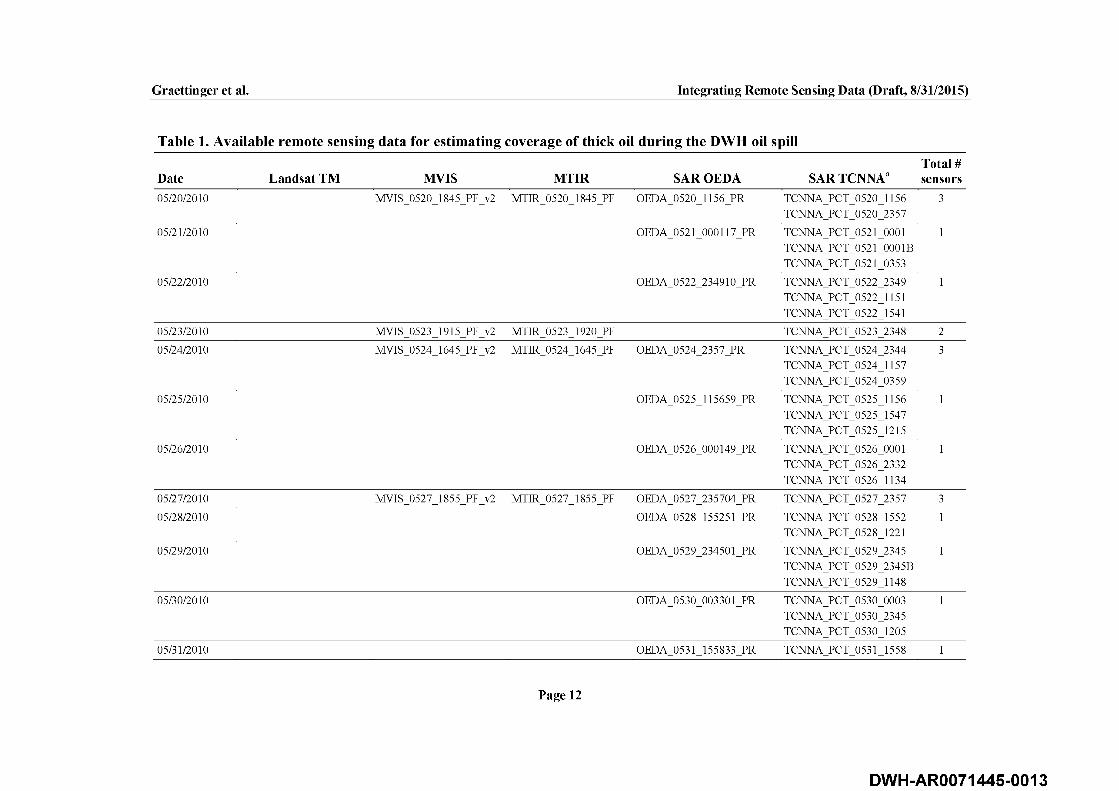
Table 1. Available remote sensing data for estimating coverage of thick oil dnring the DWH oil spillTotal #

Date Landsat TM MVIS MTIR SAR OEDA SAR TCNNA" sensors04/25/2010 MV1S_ 0425_1855_PF_v2 MT1R_0425_1855_PF OEDA_0425_1150_PR TCNNA_PCT_0425_1150 3

04/26/2010 OEDA_0426_1558_PR TCNNA_PCT_0426_15 5 8 1

04/29/2010 MV1S_ 0429_1655_PF_v2 MT1R_0429_1655_PF TCNNA_PCT_0429_0345TCNNA_PCT_0429_1209

2

05/02/2010 OEDA_0502_0351_PR TCNNA_PCT_0502_0351 1

05/03/2010 OEDA_0503_1153_PR TCNNA_PCT_0503_1153 TCNNA_PCT_0503_2357

1

05/04/2010 MVIS 0504J845_PF_v2 MT1R_0504_1850_PF OEDA_0504_2357_PR TCNNA_PCT_0504_2357 3


1


1

05/09/2010 LDST_0509_1617_PR_V2 MV1S_ 0509_1905_PF_v2 MT1R_0509_1905_PF OEDA_0509_1550_PR TCNNA_PCT_0509_1550 4

05/10/2010 MV1S_ 0510_1635_PF_v2 MT1R_0510_1635_PF OEDA_0510_2353_PR TCNNA_PCT_0510_1158 TCNNA_PCT_0510_23 5 3

3

05/11/2010 MV1S_ 0511_1855_PF_v2 OEDA_0511_1203_PR TCNNA_PCT_0511_1203 TCNNA_PCT_0511_2357

2


1

05/14/2010 OEDA_0514_1151_PR TCNNA_PCT_0514_2345 TCNNA_PCT_0514_0005 TCNNA_PCT_0514_1151

1

05/15/2010 OEDA_0515_235343_PR TCNNA_PCT_0515_23 5 3 TCNNA_PCT_0515_1209

1

05/16/2010 OEDA_0516_115720_PR TCNNA_PCT_0516_1157 1

05/17/2010 LDST_0517_1618_PR_V2 MV1S_ 0517_1640_PF_v2 MT1R_0517_1640_PF OEDA_0517_1145_PR TCNNA_PCT_0517_2348 TCNNA_PCT_0517_1145

4

Page 11

DWH-AR0071445-0012



Date Landsat TM MVIS MTIR SAR OEDA SAR TCNNA" sensors05/20/2010 MV1S_ 0520_1845_PF_v2 MT1R_0520_1845_PF OEDA_0520_1156_PR TCNNA_PCT_0520_1156

TCNNA_PCT_0520_23573

05/21/2010 OEDA_0521_000117_PR TCNNA_PCT_0521 _0001 TCNNA_PCT_0521 _0001B TCNNA_PCT_0521 _03 5 3

1


1

05/23/2010 MV1S_ 0523_1915_PF_v2 M11R_0523_1920_PF rCNNA_PCl_0523_2348 2

05/24/2010 MV1S_ 0524_1645_PF_v2 MT1R_0524_1645_PF OEDA_0524_2357_PR TCNNA_PCT_0524_2344 TCNNA_PCT_0524_1157 TCNNA_PCT_0524_03 5 9

3


1


1

05/27/2010 MV1S__0527_1855_PF_v2 MT1R_0527_1855_PF OEDA_0527_235704_PR TCNNA_PCT_0527_2357 3


1

05/29/2010 OEDA_0529_234501_PR TCNNA_PCT_0529_2345 TCNNA_PCT_0529_2345B TCNNA_PCT_0529_1148

1

05/30/2010 OEDA_0530_003301_PR TCNNA_PCT_0530_0003TCNNA_PCT_0530_2345TCNNA_PCT_0530_1205

1

05/31/2010 OEDA_0531_155833_PR TCNNA_PCT_0531_1558 1

Page 12

DWH-AR0071445-0013



Date Landsat TM MVIS MTIR SAR OEDA SAR TCNNA" sensors06/01/2010 OEDA_0601 _23 5 805_PR TCNNA_PCT_0601 _23 5 8

TCNNA_PCT_0601_11561

06/02/2010 OEDA_0602_115917_PR TCNNA_PCT_0602_1159 TCNNA_PCT_0602_1109 TCNNA_PCT_0602_1635 TCNNA_PCT_0602_1131

1


1

06/04/2010 OEDA_0604_235656_PR TCNNA_PCT_0604_2356 1

06/05/2010 OEDA_0605_114419_PR TCNNA_PCT_0605_1144 TCNNA_PCT_0605_1144B

1


1

06/07/2010 MT1R_0607_1700_PF TCNNA_PCT_0607_15 3 8 TCNNA_PCT_0607_0005

1


1

06/09/2010 OEDA_0609_2350_PR TCNNA_PCT_0609_2350TCNNA_PCT_0609_0356

1

06/10/2010 LDST_0610_1617_PR_V2 MV1S_ 0610_1905_PF_v2 MT1R_0610_1905_PF OEDA_20100610_115720_T5 TCNNA_PCT_0610_1157 4

06/12/2010 MV1S_ 0612_1850_PF_v2 MT1R_0612_1855_PF OEDA_0612_2356_PR TCNNA_PCT_0612_23 56 TCNNA_PCT_0612_2328 TCNNA_PCT_0612_0402

3


1

Page 13

DWH-AR0071445-0014



Date Landsat TM MVIS MTIR SAR OEDA SAR TCNNA" sensors06/18/2010 MV1S_ 0618_1850_PF_v2 MT1R_0618_1640_PF 2

06/19/2010 MT1R_0619_1900_PF OEDA_0619_0341_PR TCNNA_PCT_0619_0341 TCNNA_PCT_0619_1601

2

06/20/2010 MT1R_0620_1630_PF OEDA_0620_1152_PR TCNNA_PCT_0620_1152 TCNNA_PCT_0620_1144

2

06/21/2010 OEDA_0621_1613_PR TCNNA_PCT_0621 _1613 TCNNA_PCT_0621 _1613B

1

06/22/2010 OEDA_0622_034808_PR TCNNA_PCT_0622_0348TCNNA_PCT_0622_2344

1

06/23/2010 MT1R_0623_1835_PF TCNNA_PCT_0623_0032TCNNA_PCT_0623_1208

1

06/24/2010 MT1R_0624_1605_PF OEDA_0624_115 913_PR TCNNA_PCT_0624_1159 2

06/25/2010 OEDA_0625_120017_PR TCNNA_PCT_0625_1200 1

06/26/2010 LDST_0626_1617_PR_V2 MV1S_ 0626_1905_PF_v2 MT1R_0626_1905_PF OEDA_0626_1625_PR TCNNA_PCT_0626_1625 TCNNA_PCT_0626_1625B TCNNA_PCT_0626_1541

4

06/27/2010 MT1R_0627_1603_PF OEDA_0627_235234_PR TCNNA_PCT_0627_23 3 8 TCNNA_PCT_0627_1214 TCNNA_PCT_0627_1148

2

07/02/2010 OEDA_0702_115600_PR TCNNA_PCT_0702_23 32 TCNNA_PCT_0702_15 52 TCNNA_PCT_0702_1208 TCNNA_PCT_0702_1616

1


1

07/04/2010 LDST_0704_1618_PR_V2 OEDA_0704_2347_PR TCNNA_PCT_0704_2347 2

07/05/2010 OEDA_0705_1558_PR TCNNA_PCT_0705_1558 1

Page 14

DWH-AR0071445-0015



Date Landsat TM MVIS MTIR SAR OEDA SAR TCNNA" sensors07/08/2010 OEDA_0708_0344_PR TCNNA_PCT_0708_0344

TCNNA_PCT_0708_1604 TCNNA_PCT_0708_0001

1

07/10/2010 OEDA_0710_112107_PR TCNNA_PCT_0710_1121 1

07/11/2010 MT1R_0711_1645_PF OEDA_0711_0349_PR TCNNA_PCT_0711_0349 TCNNA_PCT_0711_2350 TCNNA_PCT_0711_1156 TCNNA_PCT_0711_0013

2

07/12/2010 LDST_0712_1617_PR_V2 MV1S_ 0712_1905_PP_v2 M11R_0712_1905_PF OEDA_0712_2353_PR I'CNN A_PC1 _0712_23 54 TCNNA_PCT_0712_2350

4

07/14/2010 MV1S_ 0714_1855_PF_v2 MT1R_0714_1855_PF TCNNA_PCT_0714_1152 2


1

07/17/2010 OEDA_0717_000322_PR TCNNA_PCT_0717_0032 1


1

07/20/2010 LDST_0720_1618_PR_V2 MT1R_0720_1640_PF TCNNA_PCT_0720_1108 TCNNA_PCT_0720_1214 TCNNA_PCT_0720_0038 TCNNA_PCT_0720_161 IB TCNNA_PCT_0720_1611

2

07/21/2010 MV1S_ 0721_1900_PF_v2 MT1R_0721_1900_PF OEDA_0721_1155_PR TCNNA_PCT_0721_15 5 5 TCNNA_PCT_0721_23 52

3

07/24/2010 OEDA_0724_034001 _PR TCNNA_PCT_0724_0340TCNNA_PCT_0724_1600

1

07/25/2010 OEDA_0725_0005_PR TCNNA_PCT_0725_1617 TCNNA_PCT_0725_1617B

1

Page 15

DWH-AR0071445-0016


Table 1. Available remote sensing data for estimating coverage of thick oil dnring the DWH oil spill

Date Landsat TM MVIS MTIR SAR OEDATotal #

SAR TCNNA" sensors07/26/2010 OEDA_0726_1156_PR TCNNA_PCT_0726_1156 1

TCNNA_PCT_0726_23 5 3 TCNNA_PCT_0726_0002

07/28/2010 LDST_0728_1617_PR_V2 1

Total images 8 18 25 60 142a. Some long image swaths were broken into two separate images. These images have the same date and time, with a “B” appended to one image.

Page 16

DWH-AR0071445-0017


■D

• Wellhead

Area of interestlOOKm Rn

Figure 1. Intersection of 5 km x 5 km grid with the cumulative SAR TCNNA footprint for the entire duration of the spill (ERMA, 2015). There are 6,309 cells where some oil was detected during the spill; known natural oil seeps outside of the main footprint were removed. In subsequent images, this footprint is depicted as the “area of interest.”

3. ResultsAll of the underlying imagery and the calculated coverage of thick oil and thin oil per cell are available on NOAA’s web-based Environmental Response Management Application (ERMA, 2015). This section presents summary data and figures depicting thick and thin oil priority sensors and coverage on May 17, 2010, as an example.

Cells closest to the wellhead logically had detectable thick oil on the most number of days (up to 49 of the 68 days with available data), and cells more distant from the wellhead generally had fewer days with detectable thick oil (Figure 2). Because the available data are discontinuous, the cumulative footprint of oil in Figure 2 is also discontinuous, particularly in grid cells farther from the source. Logically, the oil had to transit through some of the grid cells that are shown as being outside of the footprint, but we do not have an image that was collected when oil was in those cells.

Page 17

DWH-AR0071445-0018


I

C um yljlivs itiy s o f oiling No of d iy i _ '- 4 1 - 4*■ 31 ■ 41)

21-3D 11-20 1 - 10 D

• WsOhead C Ana •ntsfost

G (f / f a t fcfijjf f c©:

T M K m ,

SOMdM

Figure 2. Cumulative uumber of days per grid cell (out of 68 total days with available data) iu which thick oil was preseut.

May 17, 2010 was one of the few days for which we have data from all four sensors. In addition, it is the one day with AVIRIS data that have been analyzed (Clark et al., 2010). Applying the thick oil priority logic described previously to all grid cells within the area of interest, we had 1,679 cells where TM was the priority sensor, 3,220 cells where MVIS was the priority sensor, 579 cells where MTIR was the priority sensor, and 28 cells where SAR OEDA was the priority sensor (Figure 3). The remaining 803 grid cells in the area of interest are far to the west and to the southeast of the wellhead; we had no data from any sensors on May 17, 2010 from which we could estimate thick oil in those cells (Figure 3).

SAR TCNNA covered almost the entire sampled area on May 17, 2010 and thus was the priority thin sensor for the vast majority of cells (Figure 4). West of the wellhead, there was a small cluster of 12 cells where priority thin was TM, and 4 cells where priority thin was MTIR (Figure 4).

Page 18

DWH-AR0071445-0019


May 17. 2010M>n44<; T hkli

UDRtmMr/lS ( O OEDA

Harm * WeVteaa

0 lOOKm0

Figure 3. Priority sensor for estimating coverage of thick oil on May 17, 2010.

M*y 17, 2010Priodfy w n s o r : TNIn

MTIR

J Ham • MVe«n«M

Figure 4. Priority sensor for estimating coverage of thin oil on May 17, 2010. SARTCNNA was the priority thin sensor for all but a small area west of the wellhead.

Page 19

DWH-AR0071445-0020


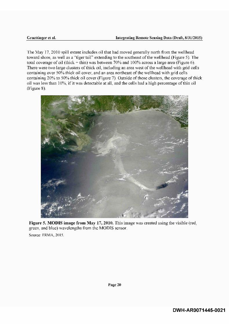
The May 17, 2010 spill extent includes oil that had moved generally north from the wellhead toward shore, as well as a “tiger tail” extending to the southeast of the wellhead (Figure 5). The total coverage of oil (thick + thin) was between 70% and 100% across a large area (Figure 6). There were two large clusters of thick oil, including an area west of the wellhead with grid cells containing over 50% thick oil cover, and an area northeast of the wellhead with grid cells containing 20% to 50% thick oil cover (Figure 7). Outside of those clusters, the coverage of thick oil was less than 10%, if it was detectable at all, and the cells had a high percentage of thin oil (Figure 8).

Figure 5. MODIS image from May 17, 2010. This image was created using the visible (red, green, and blue) wavelengths from the MODIS sensor.

Source: ERMA, 2015.

Page 20

DWH-AR0071445-0021


17.2010 Total all c o v tn g a (Wick a Win]■ I UH>901k-7<Ma

>34%-SC%>S(5%.35%s»S1k'J0%jlO » -S %0%

• vwaDwad

l O O K m ^ I

0 SOIUMes

Figure 6. Percent cover of oil of any thickness per grid ceil on May 17, 2010.

M»/ 17.2010oUcGvrngc

■ ■ >50% - 75%

- — I >15%-25% >5% - 10%

0%l O O K m _I

0 so MiIh

Figure 7. Percent cover of thick oil per grid ceil on May 17, 2010.

Page 21

DWH-AR0071445-0022


Gof f of M J C OM»y 17.2010 Thin o i cavr^ngD-

■ I>50% -60S >25%-50% >iCrH-a$% *0% - 10%

D%l O O K m ^

60 Mrtes

Figure 8. Percent cover of thin oil per grid ceil on May 17, 2010.

Similar priority sensor and oil coverage figures presented here for May 17, 2010 data are available for the remaining 67 days of data (ERMA, 2015).

4. DiscussionThe Landsat and MODIS data in this integrated surface oil model are satellite data that were analyzed in part by scaling up higher-resolution but spatially and temporally limited data from airbome sensors. Although that conceptual model is commonly used in remote sensing, the uncertainty can be high. The integrated model in this report uses satellite data to present an estimate of the coverage of thick and thin oil per grid cell per day. It is important to note that the satellite sensors cannot discern the heterogeneous nature of the oil distribution within each pixel. As a result, they may be unable to distinguish smaller patches of thick oil within a grid cell.

4.1 Spatial Heterogeneity

The DWH oil plume rose through approximately 1,500 m of water column before reaching the ocean surface. The oil rising through the water column was weathering as it rose. Once on the surface, the oil was typically sorted into relatively narrow bands of thicker oil, with more

Page 22

DWH-AR0071445-0023


widespread coverage of oil sheen (Leifer et al., 2012). Satellite imagery integrates reflectance from oil across a wide range of thicknesses within a single pixel (Figure 9). DWH oil thickness was not uniform across an area the size of an MVIS or MTIR pixel. In fact, Hu et al. (2015) show AVIRIS statistics that suggest that the reflectance value indicative o f moderately thick oil typically has 12.5% thick oil and 87.5% no oil rather than a more uniform coverage of moderate oil.

Figure 9. Spatial heterogeneity of oil. The boxes show the approximate spatial coverage of one MTIR pixel (A) and one MVIS pixel (B). Both sensors would likely classify the oil within these hypothetical pixels as thicker than thin.

Background photo source: Ocean Imaging Corp.

In addition to the heterogeneity of the oil, the water content of the oil emulsions also ranges widely over a relatively small area (Clark et al., 2010). Even if the oil thickness were uniform in a pixel, the volume of oil would vary depending on the water content of the emulsions. While discerning the oil thickness/volume in a given pixel is highly uncertain, it is clear that in MODIS and TM, reflectance in a given pixel changes when more oil is present than when less oil is present (for SAR, reflectance changes when thick, emulsified oil is present compared to when it is not). While there are no specific field data to compare with the remote sensing results, the methods developed to detect oil in these satellite images are based on data gathered previously in laboratory, mesocosm, and controlled field studies (e.g., Svejkovsky and Muskat, 2006, 2009; Clark et al., 2010; Svejkovsky and Hess, 2012; Svejkovsky et al., 2012).

Page 23

DWH-AR0071445-0024


4.2 Thickness Classes

Despite the drawbacks of oil heterogeneity and uncertainty, the methods developed as part of this NRDA work demonstrated that a large quantity of oil could be detected on the ocean surface from space, and that areas with thicker oil can be classified separately than areas with thin oil. Each of the methods developed for this study provide estimates of approximate oil volume at given reflectance levels, with “average thickness” values if that volume were spread evenly across an entire pixel (Hu et al., 2015; Leifer et al., 2015; Svejkovsky et al., 2015). We compiled all the thickness/volume data for each classification from each method.

Recognizing the uncertainty in such estimates, particularly given the known spatial heterogeneity of oil, we broadly concluded that “thin oil” can generally be considered oil with an average thickness of about 1 pm. Thicker oil ranges by orders of magnitude, varying both in thickness of oil and in percent oil in an emulsion. Across this broad spectrum, we estimate that oil classified as “thick oil” in this integrated model corresponds to a volume of oil that would have an average thickness of no less than 10 pm. This minimum estimate for average thickness of thicker oil is likely an underestimate in the best of cases, and a gross underestimate in areas near the wellhead where the thickest oil and emulsions were detected.

4.3 Validation

Synoptic sampling data were used to validate the satellite-based estimates of oiling, although available data are spatially and temporally limited. When possible, we attempted to verify the presence of detectable thick oil using photographs from a range of sources, including Ocean Imaging and NOAA photographs, and visible spectra from EPA ASPECT and WorldView-2 high-resolution satellites (hereafter referred to as “photographs” as well). Many of the available photographs were taken from an oblique viewpoint out the window of an airplane or helicopter, in which case the global positioning system (GPS) coordinates provide only the location of the camera, not the location of the oil in the picture. The location of oil in oblique pictures was estimated to the extent possible based on the data available.

Classified satellite imagery was compared to the photographs using a comparison matrix (Congalton, 1991) where the photographs are “reference data.” These matrices provide the overall photograph-to-satellite classification accuracy assessment. In general, the comparisons yielded encouraging results, with thicker oil visible from airplanes often coinciding with thicker oil classified in satellite images (Hu et al., 2015; Svejkovsky et al., 2015).

Page 24

DWH-AR0071445-0025


5. ConclusionThis model is intended to integrate the results of several independent remote sensing methods for detecting the presence of oil on the surface of the GOM during the DWH spill. Although each method represents a significant improvement in the state of the art, it is likely that each has a high degree of uncertainty. With little synoptic ground-truthing data collected during the spill, it is difficult to quantify that uncertainty. However, we have five independent methods of evaluating oil on the ocean surface (TM, MVIS, MTIR, SAR OEDA, and SAR TCNNA), using data from at least 11 different satellites, and all are in agreement that oil covered an extensive area of the surface of the northern GOM for over three months in 2010.

Our prioritization when we had multiple available sensors was based primarily on the resolution of the sensor data and the ability of the sensor to distinguish different oil thickness classes. TM was the highest priority for thick oil, but it cannot see sheens. SAR OEDA was the highest priority for total oil coverage (including thin oil and sheen), but it was the lowest priority for thick oil because it can only distinguish particularly thick, emulsified oil. By using independent data from multiple sensors, this model uses a weight-of-evidence approach to determine the presence of oil on the GOM.

AcknowledgementsSeveral people contributed greatly to the work in this report, including F. Robert Chen and Lian Feng (University of South Florida), Jay Coady and Paul Whelan (NOAA), Christopher Melton (Bubbleology Research International), and Richard Streeter (Abt Associates). This work was conducted as part of the DWH NRDA.

ReferencesBonn Agreement. 2009. Bonn Agreement Aerial Operations Handbook, 2009. London, UK. Available: http://www.bonnagreement.org/site/assets/files/1081/ba-aoh revision 2 april 2012-l.pdf. Accessed 6/4/2015.

Clark, R.N., G.A. Swayze, 1. Leifer, K.E. Livo, R. Kokaly, T. Hoefen, S. Lundeen, M. Eastwood, R.O. Green, N. Pearson, C. Sarture, 1. McCubbin, D. Roberts, E. Bradley, D. Steele, T. Ryan, and R. Dominguez. 2010. A Method for Quantitative Mapping of Thick Oil Spills Using Imaging Spectroscopy. U.S. Geological Survey Open-File Report 2010-1167.

Page 25

DWH-AR0071445-0026

http://www.bonnagreement.org/site/assets/files/1081/ba-aoh


Congalton, R.G. 1991. A review of assessing the accuracy of classifications of remotely sensed data. Remote Sensing o f Environment 37:35-46.

ERMA. 2015. Web application: Deepwater Gulf Response. Environmental Response Management Application, National Oceanic and Atmospheric Administration, Seattle, WA. Available: http://gomex.erma.noaa.gov/erma.html. Accessed 8/25/2015.

Garcia-Pineda, O., M. Rissing, R. Jones, and J. Holmes. 2015. Detection o f Oil in the Nearshore Coastal Habitats of the Gulf of Mexico during the Deepwater Horizon Oil Spill: Technical Report. Prepared for National Oceanic and Atmospheric Administration and the Louisiana Coastal Protection and Restoration Authority. August.

Garcia-Pineda, O., I.R. MacDonald, X. Li, C.R. Jackson, and W.G. Pichel. 2013a. Oil spill mapping and measurement in the Gulf of Mexico with textural classifier neural network algorithm (TCNNA). IEEE Journal o f Selected Topics in Applied Earth Observations and Remote Sensing 6(6):2517-2525.

Garcia-Pineda, O., B. Zimmer, M. Howard, W. Pichel, X. Li, and I.R. MacDonald. 2009. Using SAR images to delineate ocean oil slicks with a texture-classifying neural network algorithm (TCNNA). Canadian Journal o f Remote Sensing 35(5): 1-11.

Garcia-Pineda, O., I. MacDonald, C. Hu, J. Svejkovsky, M. Hess, D. Dukhovskoy, and S.L. Morey. 2013b. Detection of floating oil anomalies from the Deepwater Horizon oil spill with synthetic aperture radar. Oceanogi'aphy 26(2): 124-137.

Hess, M. and J. McCall. 2015. Identification and Classification of Shoreline and Marsh- Embedded Oil on the Gulf Coast during the 2010 Deepwater Horizon Oil Spill: Technical Report. Prepared for the National Oceanic and Atmospheric Administration, Seattle WA. August.

Hu, C., X. Li, and W. G. Pichel. 2011. Detection o f oil slicks using MODIS and SAR imagery. In Handbook o f Satellite Remote Sensing Image Interpretation: Applications fo r Marine Living Resources Conservation and Management, J. Morales, V. Stuart, T. Platt, and S. Sathyendranath (eds.). LU PRLSPO and lOCCG, Dartmouth, NS, Canada, pp. 21-34.

Hu, C., X. Li, W.G. Pichel, and F.L. Muller-Karger. 2009. Detection of natural oil slicks in the NW Gulf of Mexico using MODIS imagery. Geophysical Research Letters 36:L01604. doi: 10.1029/2008GL036119.

Hu, C., L. Feng, O. Garcia-Pineda, G. Graettinger, M. Hess, J. Holmes, I. Leifer, I. MacDonald, and F. Muller-Karger. 2015. Remote Sensing of Surface Oil Volume during the Deepwater Horizon Oil Spill: Scaling up AVIRIS Observations to Estimate Oiling with MODIS: Technical

Page 26

DWH-AR0071445-0027

http://gomex.erma.noaa.gov/erma.html


Report. Prepared for the National Oceanic and Atmospheric Administration, Seattle, WA. August.

Leifer, I , R. Chen, C. Melton, and F. Muller-Karger. 2015. Detection oiD eepwater Horizon oil using MODIS Mid Infrared and Thermal Infrared Imagery. Prepared for the National Oceanic and Atmospheric Administration, Seattle, WA. August.

Leifer, I , W.J. Lehr, D. Simecek-Beatty, E. Bradley, R. Clark, P. Dennison, Y.X. Hu,S. Matheson, C.E. Jones, B. Holt, M. Reif, D.A. Roberts, J. Svejkovsky, G. Swayze, and J. Wozencraft. 2012. State of the art satellite and airborne marine oil spill remote sensing: Application to the BP Deepwater Horizon oil spill. Remote Sensing o f Environment 124:185- 209.

NOAA. 2012. Open Water Oil Identification Job Aid for Aerial Observation. National Oceanic and Atmospheric Administration, Office of Response and Restoration Emergency Response Division, Seattle, WA. Version 2, Updated July 2012.

Svejkovsky, J. and M. Hess. 2012. Expanding the utility of remote sensing data for oil spill response. Photogrammetric Engineering and Remote Sensing (October): 1011-1014.

Svejkovsky, J. and J. Muskat. 2006. Real-Time Detection of Oil Slick Thickness Patterns with a Portable Multispectral Sensor. Final Report submitted to the U.S. Department of the Interior Mineral Management Service, Herndon, VA. July 31.

Svejkovsky, J. and J. Muskat. 2009. Development of a Portable Multispectral Aerial Sensor for Real-Time Oil Spill Thickness Mapping in Coastal and Offshore Waters. Prepared for the U.S. DOJ Minerals Management Service, Herndon, VA. May 14.

Svejkovsky, J., M. Hess, J. Muskat, J. McCall, and O. Garcia-Pineda. 2015. Characterization of Oil Thickness Distribution Patterns within the Deepwater Horizon Oil Spill with Aerial and Satellite Remote Sensing: Technical Report. Prepared for National Oceanic and Atmospheric Administration, Seattle, WA. August.

Svejkovsky, J., W. Lehr, J. Muskat, G. Graettinger, and J. Mullin. 2012. Operational utilization of aerial multispectral remote sensing during oil spill response: Lessons learned during the Deepwater Horizon (MC-252) spill. Photogrammetric Engineering and Remote Sensing 78(10): 1089-1102.

Page 27

DWH-AR0071445-0028


Appendix A: Sensitivity AnalysesThis integrated model of remote sensing data required several prioritizing decisions, particularly on days when multiple sensors have oil spill imagery of the GOM, and on days when we had multiple overlapping SAR images producing estimates of total oil coverage. This appendix includes additional discussion of the logic used to select a priority sensor for estimating oil cover when we had multiple sensors and multiple images available.

All images collected on a calendar day were grouped together; thus, some of the daily images were taken hours apart. This raises the possibility that the same oil could have been seen in different locations with different morphologies by different sensors on the same day. To minimize this effect, we selected the data from a single sensor per cell per day, rather than considering the data additive. In addition, we downsampled the data into a coarse grid with 25-km^ grid cells; this decreased the likelihood that a patch of oil could drift from one cell to another and be counted in two different grid cells over the course of a day.

Priority Sensor for Thick Oil

The logic for selecting the priority sensor for thick oil included two specific thresholds: use TM if TM data are available for at least 50% of the cell (or if the TM coverage is within 10% of the next highest sensor), and use MTIR if MVIS covers less than 80% of the cell.

W e conducted a sensitivity analysis on the 50% threshold for TM, comparing the thick oil results if the TM threshold were 25% or 75% (Figure A .l). The total area of thick oil is noticeably lower on May 17 and July 4, and higher on June 26, 2010, if the threshold is 75%. There is little difference on the other days, and little difference between a 25% and a 50% threshold. We concluded that the 50% threshold was reasonable.

W e also conducted a sensitivity analysis on the MVIS/MTIR threshold of 80%. Originally, we compared thresholds of 80%, 90%, and 99% (Figure A.2). It was clear from this analysis that MTIR was not capturing some of the thick oil, particularly on May 23, 2010. When the threshold for changing from MVIS to MTIR was 90% cell coverage, MVIS was the priority thick sensor for 5,324 cells, and MTIR was the priority sensor for 146 cells. When the threshold was changed from 90% to 99% cell coverage, 462 cells changed from having MVIS as the priority thick sensor to MTIR as the priority thick sensor. The total estimate of thick oil using the 99% threshold (i.e., making MTIR the priority thick sensor for many more cells) resulted in the estimate for thick oil coverage dropping to less than half the estimate using a 90% threshold, with the oil coverage then jumping back up on May 24, 2010 (Figure A.2). We concluded that MTIR was not capturing all of the thick oil on May 23, 2010 when the 99% threshold was used.

Page 28

DWH-AR0071445-0029


1200

1000

800

600

u

400

200 n I 11

J

I I\yrO

I 25% TM coverage

I50%TM coverage 175% TM coverage

/VrvV

ft'

Figure A.I. Total area of thick oil (km ) on days where TM data were available, using priority sensor thresholds of 25%,50%, and 75% TM coverage. The total area of thick oil on July 28, 2010 was about 0.3 km^ and thus is not visible at this scale.

Page 29

DWH-AR0071445-0030


1400

1200

1000

E

= 800

*5 600

400

200

MVIS 80% coverage MVIS 90% coverage

MVIS 99% coverage

o ' ^ o c v Q ? < o ^ c y c y Q ^ c y o ^ c y < ; : r Q r c r < o r Q 9 Q ^ ^ < a 9 Q r Q r o ' o' o o o

Figure A.2. Total area of thick oil (km^) on days where MODIS data were available, using priority sensor thresholds of 80%, 90%, and 99% MVIS coverage.

Page 30

DWH-AR0071445-0031


W e subsequently performed the sensitivity analysis using 70%, 80%, and 90% thresholds (Figure A.3). There was little difference between these thresholds; the total area o f thick oil over the course of the spill was 0.6% higher if the threshold was 70% instead of 80%, and 1.8% lower using a 90% threshold instead of an 80% threshold. The precise number for this threshold is not a large contributor to the overall uncertainty. We concluded that the 80% threshold was reasonable.

Priority Sensor for Thin Oil

SAR TCNNA was the priority thin oil sensor when available because of its greater sensitivity to surface oil. For the TCNNA analysis, we only included cells with 100% coverage. Therefore, we did not need to set a threshold for changing the priority thin sensor based on SAR TCNNA percent coverage. If SAR TCNNA data were available, it was the priority sensor. If not, we used the highest percent cover estimate of the remaining sensors with available data.

Although we had SAR TCNNA data for 66 of the 68 days with thick oil coverage (and one of the 2 days without any SAR data was July 28, 2010, when little oil remained on the surface), the SAR coverage sometimes overlapped poorly with the area of thick oil (see Appendix B). O f the 66 days with SAR TCNNA data, there were 11 days where other sensors covered areas that SAR TCNNA did not (including May 17, 2010, shown in Figure 5, where the priority thin sensor was TM for 12 cells and M TIR for 4 cells). Although we have not performed a sensitivity analysis of the logic for selecting the priority thin sensor when SAR TCNNA data were not available, our initial calculations suggest that only about 2% of the total area of thin oil over the 68 days was measured by a sensor other than SAR. About 25% of the thin oil estimates attributable to TM or MODIS occurred on June 18, 2010, when we had no SAR data.

Page 31

DWH-AR0071445-0032


1400

1200 ■ MVIS 70% coverage

■ MVIS 80% coverage

■ MVIS 90% coverage1000

800

600

400

200

0

Q'^Q <o^Q7<37cy<5^Q2cyCyQ^crQS' Q9crCrc3^cS^crCrCrQ>' o c> Ci'o

Figure A.3. Total area of thick oil (km ) on days where MODIS data were available, using priority sensor thresholds of 70%, 80%, and 90% MVIS coverage.

Page 32

DWH-AR0071445-0033


Appendix B: SAR ImagesThere are many different satellites collecting SAR data, and most of them targeted the northern GOM in the summer of 2010. We have images from TerraSAR-X, Envisat, Radarsat (-1 and -2), CosmoSkyMed (-1, -2, and -3), ALOS-1, and ERS-2, for example.

For simplicity, we grouped images according to the date on the image, which is in Coordinated Universal Time (UTC). On many days, multiple SAR images were analyzed for total oil cover using TCNNA (see Table 1). Often the SAR TCNNA images for one day overlapped. At most, only one of the images was analyzed for thick oil using OEDA. Several other images were analyzed for total oil cover using TCNNA, and the image used for OEDA was re-analyzed separately using TCNNA (i.e., the TCNNA analysis of the SAR image used for OEDA does not incorporate any information from the OEDA analysis).

While we had more SAR imagery than from any other sensor, there were days when those images likely underestimated oil coverage in the Gulf. SAR TCNNA coverage sometimes overlapped poorly with the area classified as thick oil using data from another sensor (Figure B .l).

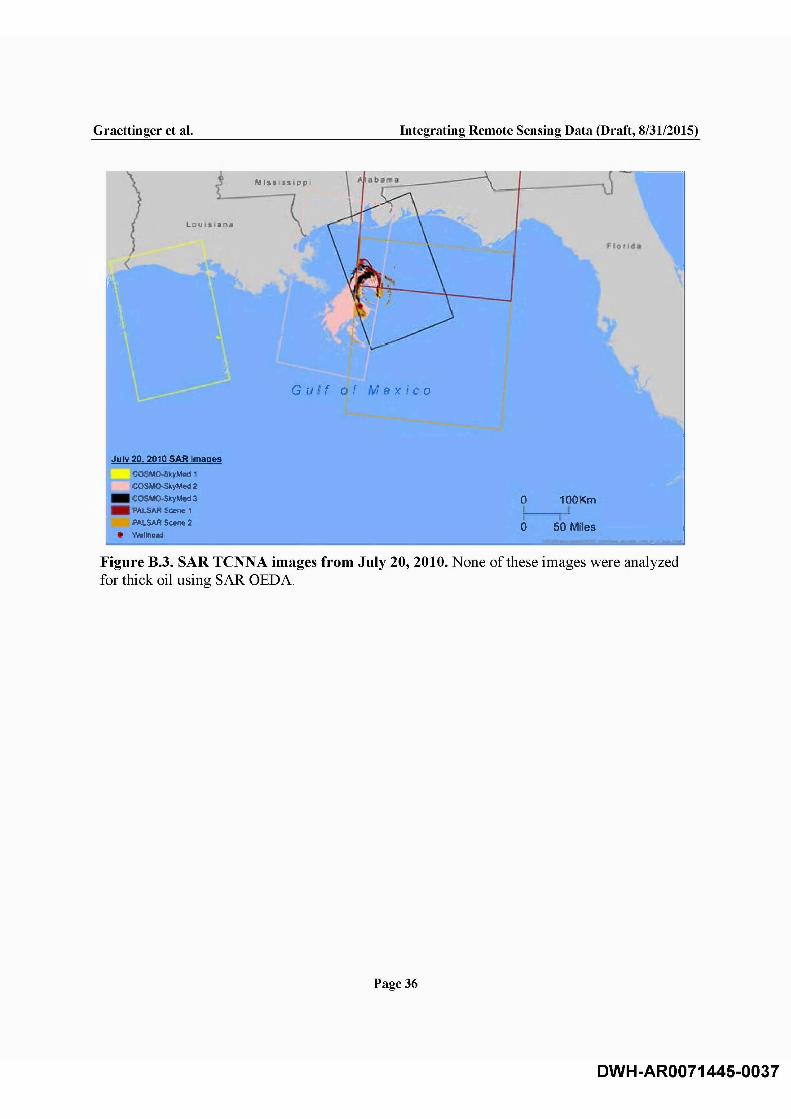
On other days, multiple SAR images were collected in a single day. The SAR images from June 2, 2010 are a good example, where only one image was used for OEDA and multiple images were used for TCNNA (Figure B.2). Another example is July 20, 2010, with five separate SAR images for TCNNA (Figure B.3), none of which was analyzed using OEDA. Some grid cells north of the wellhead were included in four of the five images.

In the SAR TCNNA logic, when a grid cell had multiple oil cover estimates from SAR TCNNA in a day, we used the highest percent cover. The sensitivity analysis to evaluate this logic was complicated by the fact that we subtract the total percent cover o f thick oil from the total percent cover of any oil by SAR TCNNA to arrive at a final estimate of percent thin oil per cell. For example, if the highest percent oil cover by SAR TCNNA was 50% and the lowest was 20%, but the estimated percent cover of thick oil (using another sensor or SAR OEDA) was 40%, the total percent thin cover would be 10% for the high estimate (50% total oil cover - 40% thick oil cover) and 0% for the low estimate (if the percent cover of thick oil is greater than the total percent oil cover by SAR TCNNA, the percent thin oil is set to 0). The net difference in the thin oil estimate is only 10%.

Page 33

DWH-AR0071445-0034


G u

Figure B .l. Area where MTIR detected thick oil (orange) compared to areal coverage of SAR TCNNA images (red outlines) on June 7, 2010. MTIR was the priority thin sensor for most of the oiled area on this day.

Page 34

DWH-AR0071445-0035


I , O U I S I ■ Bi

Florid ft

r . r . c i j S M q » - s t | « « i■ riKUr£»2

TftKftSJiR-*■ iMLSAn□ Sftntoi to9«n<t• VWOftd

lOOKm—

SOMilen

Figure B .l. SAR TCNNA images from June 2, 2010. Only one of the four images (TerraSAR-X) was analyzed for thick oil using SAR OEDA. Where images overlap, we selected the highest percent thin oil per grid cell per day. We then subtracted the percent of thick oil from the SAR TCNNA estimate of percent oil cover to arrive at a final estimate of percent thin oil per cell.

Page 35

DWH-AR0071445-0036


M I » i 11 » t p p ;|

%

A%

L q u a n i

c-

%

if V. :-K ■■ti

■'1"f

■5',

J i

I A l f l p s m g

G i i f f o f '/> » X f c 0

July 20.2010 SAfi ImagesCO$MOw$kyMed 1 COSIUDkyWed 2 COSUO-SlcylM 3 i SA.R Saev« 1 ftM.SARS«-w2

• VAIthoad

0 IQOKm

0 50 Miles

Figure B.3. SAR TCNNA images from July 20, 2010. None of these images were analyzed for thick oil using SAR OEDA.

Page 36

DWH-AR0071445-0037


Appendix C: Oil IntensityTo help clarify the appearance of “thick oil” and “thin oil” during the spill, we developed an “oil intensity index” job aid, with a description and example photographs. This index of oil intensity is intended to show examples of the diversity of oil morphologies and the variety of oil thicknesses to which natural resources may have been exposed during the spill. Four example classes of intensity are:

1. Thin/sheen oil only (Figures C. 1 and C.2)2. Mostly thin oil, with < 5% thick oil present (Figures C.3 and C.4)3. Thin oil with about 5-10% thick oil present (Figures C.5 and C.6)4. Thin oil with > 10% thick oil present (Figures C.7 through C.9).

It is important to note that the photographs for each class are typically not showing the entire area of a 5 km x 5 km grid cell. Many are oblique, so we cannot include a scale. However, they show examples of these four different intensity classes within the field of view of the photograph.

Page 37

DWH-AR0071445-0038


EPA ASPECT - 05 09 2010

0 55 110 330 440Meters

EPA ASPECT^ 05/17/2010

0 125 250 500 750 1,000M eters

Figure C .l. Examples of thin/sheen oil only (intensity class 1). The scale was derived from EPA ASPECT geospatial information.

Page 38

DWH-AR0071445-0039


0 -1 8 75 -37 .5 -7 5 -112.5 -150Meters

Figure C .l. Additional examples of thin/sheen oil only (intensity class 1). The scale in the upper photograph was estimated by assuming the average length of an oil spill response vessel is about 60 m.

Page 39

DWH-AR0071445-0040


0 1B7.5 375 750 1125 1500Meters

,120011645hrsl®ni5Sii2E0M ississippi

@37

if ^

Figure C.3. Examples of thin oil with < 5% thick oil present (intensity class 2). The upper photograph shows both oil and sediment in the water around an island; the scale is estimated based on the size of features on the island.

Page 40

DWH-AR0071445-0041


EPAAS P E C T -05/09/2010

Vieters

Figure C.4. Additional examples of thin oil with < 5% thick oil present (intensity class 2).The images show larger areas o f thin oil with narrow strands of thick oil. The scale of the upper image was derived from EPA ASPECT geospatial information. The lower image is from Ocean Imaging’s georeferenced imagery.

Page 41

DWH-AR0071445-0042


62,5 -125 -2 5 0Meters

52,5 -125Meiers

Figure C.5. Examples of thin oil with about 5-10% thick oil present (intensity class 3). Thescales in the images were estimated from features such as response vessels, assuming the average length of a vessel is about 60 m.

Page 42

DWH-AR0071445-0043


O verflight

CDSPB3EQ5P0rs.17.9!@10 'p1 : iT3

0 5 / . 1 r7 / 2 0 1 0

Deepwater, O v erf l ig h t

06/10/2010

Figure C.6. Additional examples of thin oil with ahont 5-10% thick oil present (intensity class 3).

Page 43

DWH-AR0071445-0044


Mississippi]

w m F m mM e t e r s

05/iro2010 66)^0 HZ3

05/12/2010-8:35am CSX

C op y rig h t 2010 O c ean Im ag ing N ot fo r public d istribu tion

Figure C.7. Examples of thin oil with at least 10% thick oil present (intensity class 4). Thescales in the images were estimated from features in the images. The lower image is from Ocean Imaging’s georeferenced imagery.

Page 44

DWH-AR0071445-0045


0 'is/.s-i/s -1 1 ^ 5 -1500Meters

. __

Figure C.8. Additional examples of thin oil with at least 10% thick oil present (intensity class 4). The scale in the top image was estimated from features such as response vessels, assuming the average length of a vessel is about 60 m.

Page 45

DWH-AR0071445-0046


Figure C.9. Additional examples of thin oil with at least 10% thick oil present (intensity class 4).

Page 46

DWH-AR0071445-0047

Documents

Integrating Data from Mnltiple Satellite Sensors to