Research ArticleIntegrated Workflow of Geomechanics, Hydraulic Fracturing, andReservoir Simulation for Production Estimation of a ShaleGas Reservoir

Taeyeob Lee,1 Daein Jeong,2 Youngseok So,1 Daejin Park,1 Munseok Baek,1

and Jonggeun Choe 3

1E&P Research Center, Korea Gas Corporation, 41062, Republic of Korea2Schlumberger Information Solutions, Schlumberger, 103-0027, Japan3Department of Energy System Engineering, Seoul National University, 08826, Republic of Korea

Correspondence should be addressed to Jonggeun Choe; johnchoe@snu.ac.kr

Received 25 August 2020; Revised 30 September 2020; Accepted 31 March 2021; Published 27 April 2021

Academic Editor: Basim Abu-Jdayil

Copyright © 2021 Taeyeob Lee et al. This is an open access article distributed under the Creative Commons Attribution License,which permits unrestricted use, distribution, and reproduction in any medium, provided the original work is properly cited.

In this research, an integrated workflow from geomechanics to reservoir simulation is suggested to accurately estimateperformances of a shale gas reservoir. Rather than manipulating values of hydraulic fracturing such as fracture geometry andtransmissibility, the workflow tries to update model parameters to derive reliable hydraulic fracturing results. A mechanicalearth model (MEM) is built from seismic attribute and drilling and diagnostic fracture injection test results. Then, the MEM iscalibrated with microseismic measurements obtained in a field. Leakoff coefficient and horizontal stress anisotropy are sensitiveparameters of the MEM that influence the propagation of the fracture network and gas productions. Various combinations ofcalibration parameters from a single-well simulation are evaluated. Then, an appropriate combination is chosen from the wholesimulation results of a pad to reduce the uncertainty. Finally, production estimations of the four wells which have slightlydifferent fracture design are compared with seven-year production history. Their results are reasonably matched with actual datahaving 8% of global error due to successful development of the reservoir model with geomechanical parameters.

1. Introduction

Advancements in horizontal well drilling and multistagehydraulic fracturing have enabled economically viable gasproductions from shale formations. Predicting productionsof a fractured shale reservoir is essential for field assessmentsand establishing an optimum development plan. In the lastdecade, there have been a lot of researches to predict perfor-mances of shale gas reservoirs using a numerical simulation.It incorporates geological, geomechanical, and petrophysicalproperties and examines their effects on gas productions.Therefore, it will be more robust than analytical or empiricalmethods.

Numerical simulations in shale reservoirs could be catego-rized into two groups. One method is to use only a reservoirsimulation model, and hydraulic fracture (HF) parameterssuch as fracture height and half-length are considered uncer-

tain parameters. Nejadi et al. [1] presented a novel approachfor characterization and history matching of hydrocarbonproduction from a hydraulic fractured shale gas. They usedan assisted history matching algorithm to compare produc-tion performances with actual responses and updated HFand discrete fracture network (DFN) model parameters.Their approach could characterize fracture parameters.However, it is limited on the specific fracture design whichwas done already.

Yu et al. [2] performed a multistage fractured horizontalwell numerical simulation on the basis of reservoir propertiesand completion parameters from an actual horizontal explo-ration well in China. They analyzed the effect on multistagefractured horizontal well’s performances for matrix perme-ability, permeability of stimulated reservoir volume (SRV),HF conductivity and half-length, SRV size, and bottomholepressure. Their approach has some limitations since the

HindawiGeofluidsVolume 2021, Article ID 8856070, 17 pageshttps://doi.org/10.1155/2021/8856070

method does not consider the relationship between fracturedesigns and the resulting fracture parameters.

Chang and Zhang [3] proposed a method for characteriz-ing the SRV of shale gas reservoirs using production data.They treated major-fracture properties, the spatial extent ofthe SRV, and the properties of a dual-porosity, dual-permeability model as uncertain parameters. Using an itera-tive ensemble smoother, they performed the history matchingand suggested the updated values of uncertain parameters.They tried to estimate shale gas productions in a stochasticapproach. However, it is based on a synthetic model withoutconsidering actual hydraulic fracturing results.

The other method is to integrate a HF simulation and thereservoir simulation model. This method tries to describe HFpropagations and their impacts on gas productions. Ajisafeet al. [4] applied a multidisciplinary integrated workflow toa horizontal well to model complex HFs and gas productions.They input the DFN and geomechanical properties into theunconventional fracture model (UFM) and calibrated themwith the microseismic data and production history. Theirapproach was limited to the single-well application.

Cipolla et al. [5] illustrated an application of two complexfracture modelling techniques in conjunction with microseis-mic mapping to characterize fracture complexity and evalu-ated completion performances. The authors tried to matchthe fracture propagation results with measured microseismicmapping based on the various combinations of stress anisot-ropies and natural fracture spacing. They only focused on thefracture shape (fracture length and complexity) without con-sidering the production performances.

Izadi et al. [6] carried out an integrated subsurface studyin a tight gas field to evaluate the stimulation process in hor-izontal wells. They utilized all available data to build a 3Dgeomechanical model and tried to quantify heterogeneousin situ stress effects on HF propagation and stimulation effi-ciency using a 3D fully coupled hydraulic fracturing simula-tor. However, this method neglected calibration processessuch as matching the results with microseismic or produc-tion data to reduce the uncertainties of the estimated geome-chanical properties.

Lee et al. [7] constructed a numerical reservoir modelbased on an integrated workflow for modelling an unconven-tional reservoir. They investigated both fracture closure andproppant placement effects. Then, they concluded that theboth parameters need to be considered to estimate gas pro-ductions in a shale gas well. They adopted the integratedworkflow from a static modelling and carried out fracturesimulation and production estimation in the same platform.However, the proposed method is still limited to a single-well analysis rather than incorporating multiple wells in apad for comprehensive analysis.

Pankaj et al. [8] used an integrated modelling workflowto determine well spacing and well-to-well interference forthe Marcellus Shale. Based on a geomechanical model, theysimulated HF propagations. After that, they calibrated themwith microseismic and well production data by varyingparameters such as horizontal stress anisotropy, fracturingfluid leakoff, and the DFN. After that, they did well spacingsensitivity to reveal an optimum distance that the wells need

to be spaced to maximize recovery and the number of wellsper section. However, they only used interpreted verticallog data to construct the geomechanical model so they didnot consider spatial heterogeneity of mechanical properties.

In this study, a novel workflow of geomechanics, hydrau-lic fracturing, and reservoir simulation is suggested for ashale gas reservoir. The workflow focuses on derivinghydraulic fracturing results which are similar to microseismicdata in terms of their geometries and also matched with gasproduction data. It gives much consistent results thanmanipulating values of hydraulic fracturing to match mea-sured data. The proposed workflow is verified in an actualpad having four wells of slightly different fracture designs.

A geomechanical model is constructed using drillingresults, diagnostic fracture injection test (DFIT) analysis,and seismic attribute data. Rock mechanical properties arecalculated from seismic attribute. Reservoir pressure is dis-tributed based on the given borehole information: drillingmud densities and the result of DFIT analysis. After that, clo-sure stress is computed using the above parameters, and it isverified with DFIT results. DFIT analysis also gives informa-tion of leakoff coefficients, and these values are used in thecalibration of the model. During the calibration, uncertainparameters being difficult to obtain are derived and validated.Finally, gas productions of a whole well pad in the shale res-ervoir are estimated using the developed workflow and com-pared with actual production data for validation.

2. Materials and Methods

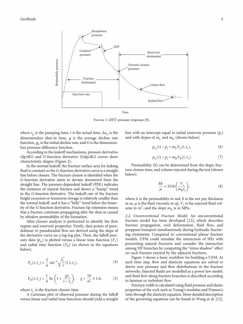
2.1. Diagnostic Fracture Injection Test. The diagnostic frac-ture injection test is useful to infer geomechanical propertiesincluding fracture closure stress, reservoir pressure, leakoffcoefficient, and permeability. A small volume of fluid isinjected into the formation, and it creates a hydraulic frac-ture. After the injection, the pressures in the wellbore aremonitored for several days and these data are analyzed usingspecial plots. A typical DFIT sequence is shown in Figure 1.

The analysis of DFIT data is conducted in two ways:before-closure analysis and after-closure analysis. Before-closure analysis focuses on the early pressure falloff periodand provides fracture closure stress, instantaneous shut-inpressure (ISIP), and leakoff mechanism and coefficient.When the surface injection is stopped, the friction decreasesrapidly and ISIP could be derived which is the sum of closurestress and net pressure. ISIP is estimated by placing a straightline on the pressure falloff plot.

Nolte [10] suggested a G-function, which is a dimension-less measure of time to investigate the pressure declinebehaviour (as shown in the equations below).

ΔtD =t − tptp

, ð1Þ

g ΔtDð Þ = 43 1+ΔtDð Þ1:5 − ΔtDð Þ1:5� �

, ð2Þ

G ΔtDð Þ = 4π

g ΔtDð Þ − g0½ �, ð3Þ

2 Geofluids

where tp is the pumping time, t is the actual time, ΔtD is thedimensionless shut-in time, g is the average decline ratefunction, g0 is the initial decline rate, and G is the dimension-less pressure difference function.

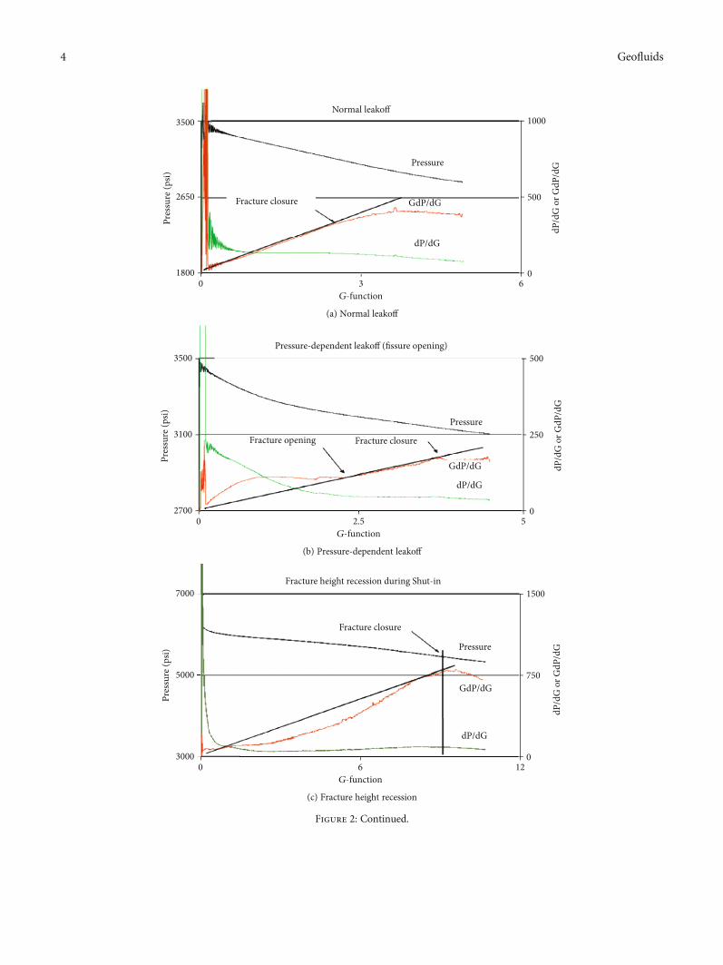
According to the leakoffmechanisms, pressure derivative(dp/dG) and G-function derivative (Gdp/dG) curves showcharacteristic shapes (Figure 2).

In the normal leakoff, the fracture surface area for leakingfluid is constant so theG-function derivative curve is a straightline before closure. The fracture closure is identified when theG-function derivative starts to deviate downward from thestraight line. The pressure-dependent leakoff (PDL) indicatesthe existence of natural fracture and shows a “hump” trendin the G-function derivative. The leakoff rate of the fractureheight recession or transverse storage is relatively smaller thanthe normal leakoff, and it has a “belly” trend below the linear-ity of the G-function derivative. Fracture tip extension meansthat a fracture continues propagating after the shut-in causedby ultralow permeability of the formation.

After-closure analysis is performed to identify the flowregime and reservoir properties. Firstly, data points of pseu-dolinear or pseudoradial flow are derived using the slope ofthe derivative curve on a log-log plot. Then, the falloff pres-sure data (pw) is plotted versus a linear time function (FL)and radial time function (FR) (as shown in the equationsbelow).

FL t, tcð Þ = 2πsin−1

ffiffiffiffitct

rt ≥ tcð Þ, ð4Þ

FR t, tcð Þ = 14 ln 1 + χtc

t − tc

� �, χ = 16

π2 ≅ 1:6, ð5Þ

where tc is the fracture closure time.A Cartesian plot of observed pressure during the falloff

versus linear and radial time functions should yield a straight

line with an intercept equal to initial reservoir pressure (pi)and with slopes of mL and mR (shown below).

pw tð Þ − pi =mLFL t, tcð Þ, ð6Þ

pw tð Þ − pi =mRFR t, tcð Þ: ð7ÞPermeability (k) can be determined from the slope, frac-

ture closure time, and volume injected during the test (shownbelow):

khμ

= 3316 Vi

mRtc

� �, ð8Þ

where k is the permeability in md, h is the net pay thicknessin m, μ is the fluid viscosity in cp, V i is the injected fluid vol-ume in m3, and the slope mR is in MPa.

2.2. Unconventional Fracture Model. An unconventionalfracture model has been developed [12], which describesfracture propagation, rock deformation, fluid flow, andproppant transport simultaneously during hydraulic fractur-ing treatments. Compared to conventional planar fracturemodels, UFM could simulate the interaction of HFs withpreexisting natural fractures and consider the interactionamong HF branches by computing the “stress shadow” effecton each fracture exerted by the adjacent fractures.

Figure 3 shows a basic workflow for building a UFM. Ateach time step, flow and elasticity equations are solved toderive new pressure and flow distributions in the fracturenetworks. Injected fluids are modelled as a power law model,and fluid flow along fracture branches is described accordingto laminar or turbulent flow.

Fracture width is calculated using fluid pressure and elasticproperties of the rock such as Young’s modulus and Poisson’sratio through the elasticity equation.More detailed descriptionof the governing equations can be found in Weng et al. [12].

Cushionpressure

Fracturedominated

ISIP

Reservoirdominated

Fracture closurepressure

Linear flow

Radial flow

Time

Injection rate

Botto

mho

le p

ress

ure

Breakdownpressure

Figure 1: DFIT pressure response [9].

3Geofluids

18000 3

G-function

Normal leakoff

dP/dG

GdP/dG

Pressure

Fracture closure

60

500

1000

2650

Pres

sure

(psi)

dP/d

G o

r GdP

/dG

3500

(a) Normal leakoff

27000 2.5

G-function

Pressure-dependent leakoff (fissure opening)

dP/dG

GdP/dG

Pressure

Fracture closureFracture opening

50

250

500

3100

Pres

sure

(psi)

dP/d

G o

r GdP

/dG

3500

(b) Pressure-dependent leakoff

30000 6

G-function

Fracture height recession during Shut-in

dP/dG

GdP/dG

Pressure

Fracture closure

120

750

1500

5000

Pres

sure

(psi)

dP/d

G o

r GdP

/dG

7000

(c) Fracture height recession

Figure 2: Continued.

4 Geofluids

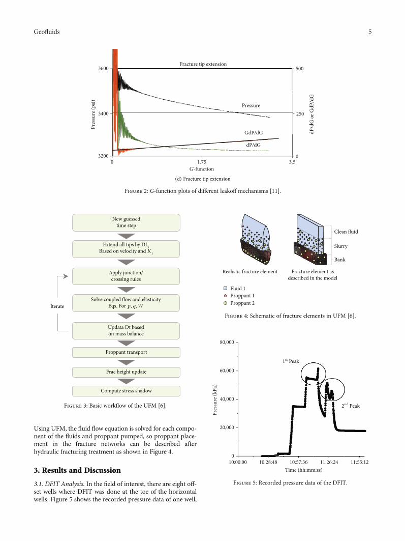
Using UFM, the fluid flow equation is solved for each compo-nent of the fluids and proppant pumped, so proppant place-ment in the fracture networks can be described afterhydraulic fracturing treatment as shown in Figure 4.

3. Results and Discussion

3.1. DFIT Analysis. In the field of interest, there are eight off-set wells where DFIT was done at the toe of the horizontalwells. Figure 5 shows the recorded pressure data of one well,

32000 1.75

G-function

Fracture tip extension

dP/dG

GdP/dG

Pressure

3.50

250

500

3400

Pres

sure

(psi)

dP/d

G o

r GdP

/dG

3600

(d) Fracture tip extension

Figure 2: G-function plots of different leakoff mechanisms [11].

Apply junction/crossing rules

Proppant transport

Frac height update

Compute stress shadow

Iterate

New guessedtime step

Extend all tips by DLiBased on velocity and K1

Solve coupled flow and elasticityEqs. For p, q, W

Updata Dt basedon mass balance

Figure 3: Basic workflow of the UFM [6].

Realistic fracture element Fracture element asdescribed in the model

Clean fluid

Slurry

Bank

Proppant 1Proppant 2

Fluid 1

Figure 4: Schematic of fracture elements in UFM [6].

010:00:00 10:28:48 10:57:36

Time (hh:mm:ss)11:26:24

2nd Peak

1st Peak

11:55:12

20,000

40,000

Pres

sure

(kPa

)

60,000

80,000

2nd Peak

1 Peak

Figure 5: Recorded pressure data of the DFIT.

5Geofluids

and it could be seen that there are two pressure peaks in theplot. Because a pressure-activated rupture disc valve isinstalled in the toe stage, pressure data after the 2nd peakshould be used to analyze.

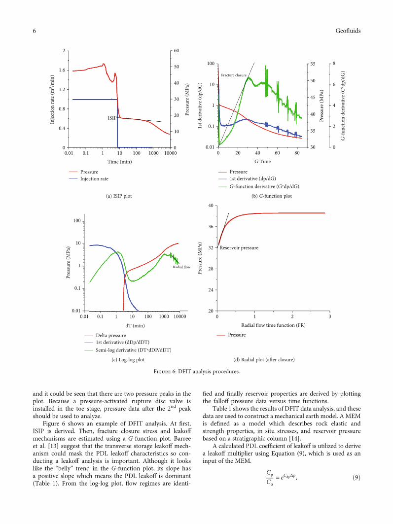
Figure 6 shows an example of DFIT analysis. At first,ISIP is derived. Then, fracture closure stress and leakoffmechanisms are estimated using a G-function plot. Barreeet al. [13] suggest that the transverse storage leakoff mech-anism could mask the PDL leakoff characteristics so con-ducting a leakoff analysis is important. Although it lookslike the “belly” trend in the G-function plot, its slope hasa positive slope which means the PDL leakoff is dominant(Table 1). From the log-log plot, flow regimes are identi-

fied and finally reservoir properties are derived by plottingthe falloff pressure data versus time functions.

Table 1 shows the results of DFIT data analysis, and thesedata are used to construct a mechanical earth model. AMEMis defined as a model which describes rock elastic andstrength properties, in situ stresses, and reservoir pressurebased on a stratigraphic column [14].

A calculated PDL coefficient of leakoff is utilized to derivea leakoff multiplier using Equation (9), which is used as aninput of the MEM.

CpCo

= eCdpΔp, ð9Þ

00.01 0.1 1 10

Time (min)

ISIP

100 1000 100000

10

20

30

40

50

60

0.4

0.8

1.2

Inje

ctio

n ra

te (m

3 /min

)

1.6

2

PressureInjection rate

Pres

sure

(MPa

)

(a) ISIP plot

0.01

1st d

eriv

ativ

e (dp

/dG

)

G-fu

nctio

n de

rivat

ive (G

⁎dp

/dG

)

Pres

sure

(MPa

)

0.1

1

10

100

0 20 40 60 8030

35

40

45

50

55

G Time

Fracture closure

Pressure1st derivative (dp/dG)G-function derivative (G⁎dp/dG)

0

2

4

6

8

(b) G-function plot

0.01

Pres

sure

(MPa

)

0.1

1

10

100

0.01 0.1 1 10

dT (min)

100 1000 10000

Delta pressure1st derivative (dDp/dDT)Semi-log derivative (DT⁎dDP/dDT)

Radial flowRadi

(c) Log-log plot

Pres

sure

(MPa

)

Pressure

20

24

28

32

36

40

Reservoir pressure

0 1 2Radial flow time function (FR)

3

(d) Radial plot (after closure)

Figure 6: DFIT analysis procedures.

6 Geofluids

where Cp is the altered leakoff coefficient, Co is the originalmatrix leakoff coefficient, Cp/Co is the leakoff multiplier,Cdp is the PDL coefficient of leakoff, and Δp is the netpressure.

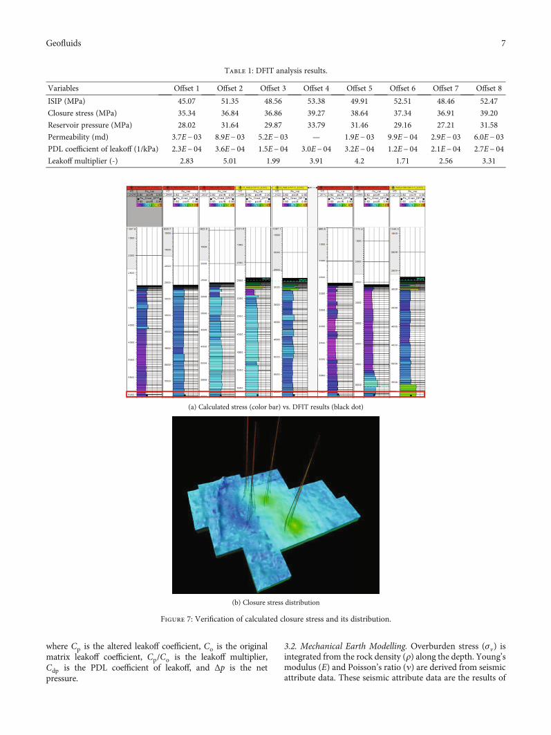
3.2. Mechanical Earth Modelling. Overburden stress (σv) isintegrated from the rock density (ρ) along the depth. Young’smodulus (E) and Poisson’s ratio (ν) are derived from seismicattribute data. These seismic attribute data are the results of

(a) Calculated stress (color bar) vs. DFIT results (black dot)

(b) Closure stress distribution

Figure 7: Verification of calculated closure stress and its distribution.

Table 1: DFIT analysis results.

Variables Offset 1 Offset 2 Offset 3 Offset 4 Offset 5 Offset 6 Offset 7 Offset 8

ISIP (MPa) 45.07 51.35 48.56 53.38 49.91 52.51 48.46 52.47

Closure stress (MPa) 35.34 36.84 36.86 39.27 38.64 37.34 36.91 39.20

Reservoir pressure (MPa) 28.02 31.64 29.87 33.79 31.46 29.16 27.21 31.58

Permeability (md) 3.7E− 03 8.9E− 03 5.2E− 03 — 1.9E− 03 9.9E− 04 2.9E− 03 6.0E− 03PDL coefficient of leakoff (1/kPa) 2.3E− 04 3.6E− 04 1.5E− 04 3.0E− 04 3.2E− 04 1.2E− 04 2.1E− 04 2.7E− 04Leakoff multiplier (-) 2.83 5.01 1.99 3.91 4.2 1.71 2.56 3.31

7Geofluids

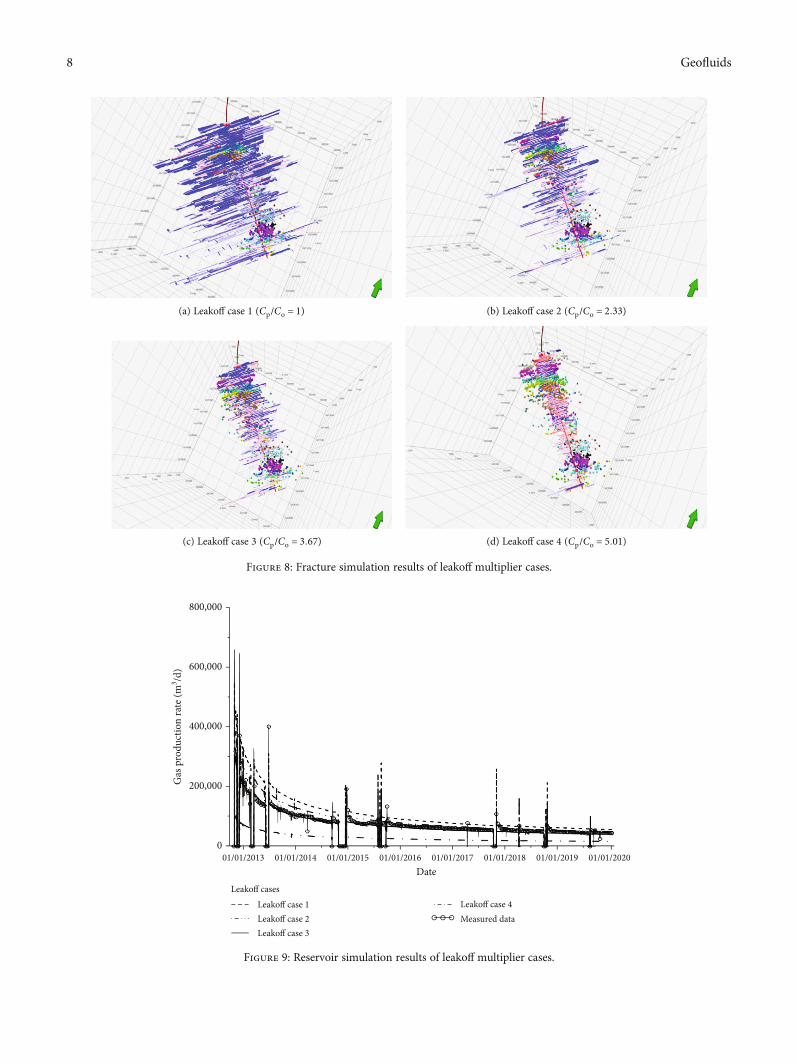
(a) Leakoff case 1 (Cp/Co = 1) (b) Leakoff case 2 (Cp/Co = 2:33)

(c) Leakoff case 3 (Cp/Co = 3:67) (d) Leakoff case 4 (Cp/Co = 5:01)

Figure 8: Fracture simulation results of leakoff multiplier cases.

001/01/2013 01/01/2014 01/01/2015 01/01/2016

Date01/01/2017 01/01/2018 01/01/2019 01/01/2020

200,000

400,000

Gas

pro

duct

ion

rate

(m3 /d

) 600,000

800,000

Leakoff casesLeakoff case 1Leakoff case 2Leakoff case 3

Leakoff case 4Measured data

Figure 9: Reservoir simulation results of leakoff multiplier cases.

8 Geofluids

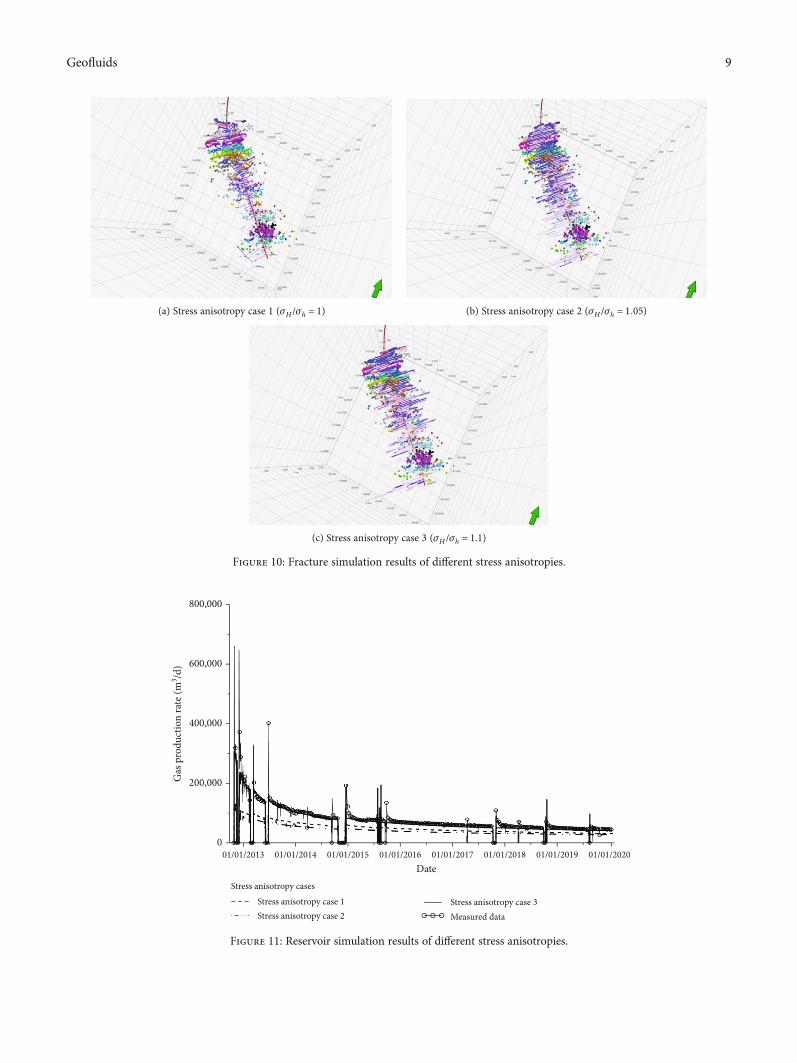
(a) Stress anisotropy case 1 (σH/σh = 1) (b) Stress anisotropy case 2 (σH/σh = 1:05)

(c) Stress anisotropy case 3 (σH /σh = 1.1)

Figure 10: Fracture simulation results of different stress anisotropies.

001/01/2013 01/01/2014 01/01/2015 01/01/2016

Date01/01/2017 01/01/2018 01/01/2019 01/01/2020

200,000

400,000

Gas

pro

duct

ion

rate

(m3 /d

) 600,000

800,000

Stress anisotropy casesStress anisotropy case 1Stress anisotropy case 2

Stress anisotropy case 3Measured data

Figure 11: Reservoir simulation results of different stress anisotropies.

9Geofluids

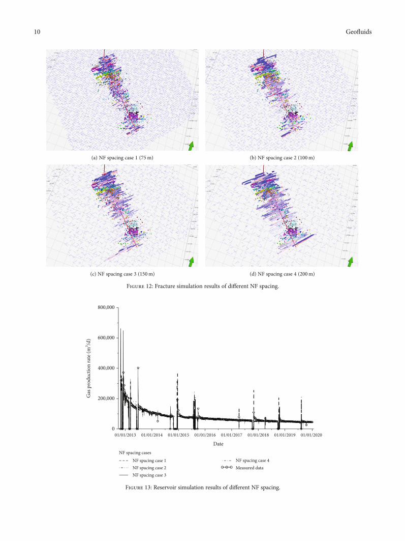
(a) NF spacing case 1 (75m) (b) NF spacing case 2 (100m)

(c) NF spacing case 3 (150m) (d) NF spacing case 4 (200m)

Figure 12: Fracture simulation results of different NF spacing.

001/01/2013 01/01/2014 01/01/2015 01/01/2016

Date01/01/2017 01/01/2018 01/01/2019 01/01/2020

200,000

400,000

Gas

pro

duct

ion

rate

(m3 /d

) 600,000

800,000

NF spacing casesNF spacing case 1NF spacing case 2NF spacing case 3

NF spacing case 4Measured data

Figure 13: Reservoir simulation results of different NF spacing.

10 Geofluids

seismic inversion analysis. During the inversion analysis, welllog data are used to calibrate the inversion results with mea-sured data.

E =ρV2

s 3V2p − 4V2

s

� �V2

p −V2s

,

ν =V2

p − 2V2s

2 V2p −V2

s

� � ,ð10Þ

where Vp and Vs are the p-wave and the s-wave velocities,respectively.

Reservoir pressure (pr) is distributed based on the givenborehole information: drilling mud densities and the resultof DFIT analysis. Finally, closure stress (σc) equivalent tominimum horizontal stress is computed from Equation (11)using the above parameters.

σc =ν

1 − νσv − αprð Þ + αpr + σt, ð11Þ

where α is the Biot constant and σt is the tectonic stress.In Figure 7(a), calculated closure stress (color bar) was

compared with the results of DFIT analysis (black dot). DFITwas performed only in the toe stage of the horizontal wells, sothere is one measured point per well. Computed stress is wellmatched with the DFIT results among the offset wells, and itsdistribution is shown in Figure 7(b). In addition, the direc-tion of the maximum horizontal stress was estimated asN45E from a world stress map and microseismic results.

However, there are still some uncertain parameters of theMEM such as leakoff coefficient, horizontal stress anisotropy,and natural fracture property. By comparing HF and reservoirsimulation results with field measured data, these uncertainparameters are calibrated and the updated MEM is obtained.

3.3. Mechanical Earth Model Calibration. The calibrationprocess was conducted for a single well, and then, it wasexpanded to a whole pad scale including the four wells.Firstly, four leakoff multiplier cases were constructed fromthe DFIT analysis. Using Equation (9), leakoff multipliers

of offset wells were estimated as shown in Table 1. Duringthe calculation, net pressure was assumed as 4.68MPa whichis the average value from hydraulic fracturing simulation. Case1 assumed that there was not any PDL leakoff effect, and othercases were constructed from the range of leakoff multipliers.Hydraulic fracturing simulations were performed and com-pared with recorded microseismic data in the field. Microseis-mic data will give a rough implication of the generated fracturegeometry. In case 3 of Figure 8, simulated fracture geometry iswell matched with microseismic data and it is also identified inthe history matching result in Figure 9.

Horizontal stress anisotropy means the difference betweenthe maximum and the minimum horizontal stresses. Sincemeasurement of the maximum horizontal stress is notdirectly possible, three different anisotropies were assumedin this research: the same with the minimum horizontalstress (case 1), 5% higher (case 2), and 10% higher (case 3).

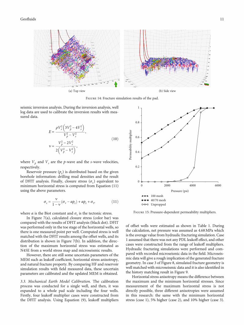
(a) Top view (b) Side view

Figure 14: Fracture simulation results of the pad.

00 2000 4000

Pressure (psi)

6000

0.2

0.4

Perm

eabi

lity

mul

tiplie

r

0.6

0.8

1

100 mesh40/70 meshUnpropped

Figure 15: Pressure-dependent permeability multipliers.

11Geofluids

001/01/2013 01/01/2014 01/01/2015 01/01/2016

Date01/01/2017 01/01/2018 01/01/2019 01/01/2020

1,000

2,000

Tubi

ng h

ead

pres

sure

(psi)

3,000

4,000

Well 1Tubing head pressureMeasured data

001/01/2013 01/01/2014 01/01/2015 01/01/2016

Date01/01/2017 01/01/2018 01/01/2019 01/01/2020

1,000

2,000

Tubi

ng h

ead

pres

sure

(psi)

3,000

4,000

Well 2Tubing head pressureMeasured data

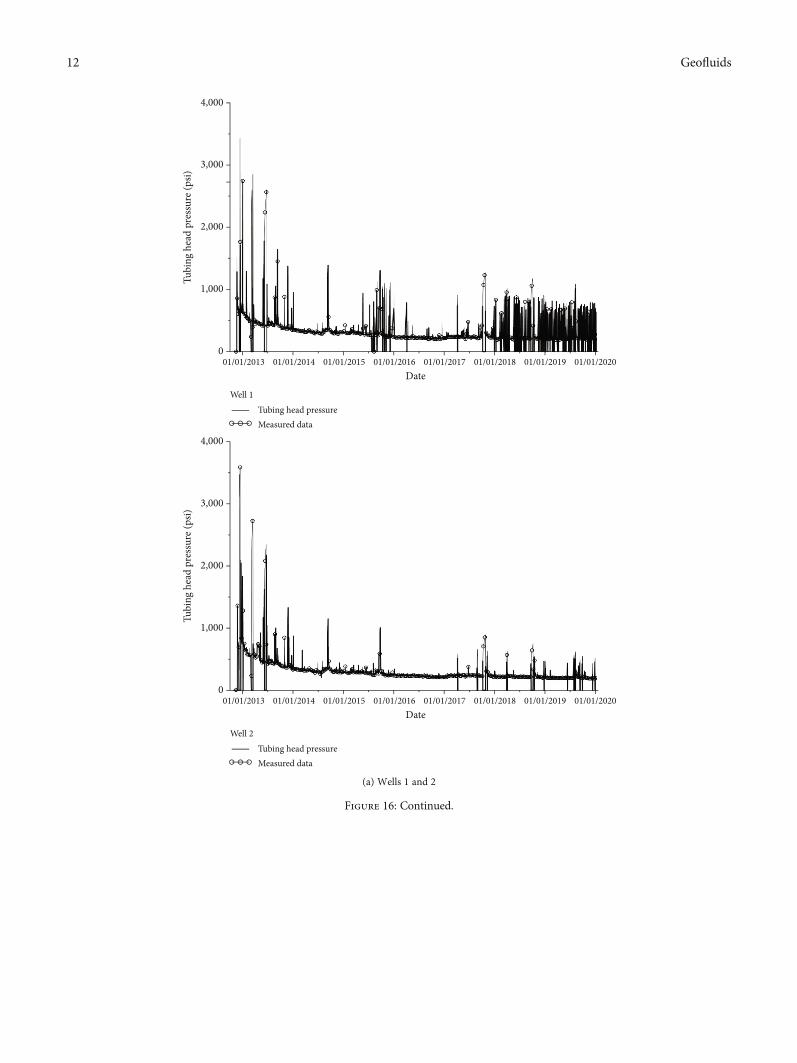
(a) Wells 1 and 2

Figure 16: Continued.

12 Geofluids

These anisotropy ranges are estimated from a correlationbetween a breakdown pressure and the maximum horizontalstress using DFIT data. The anisotropy affects both fracturegeometry and gas production rates. Figure 10 shows HF sim-ulation results of the three cases, and the shapes of case 2 andcase 3 are similar to the microseismic data which alignedalong the maximum horizontal stress direction. However,case 2 shows much lower gas production rates compared tothe actual production data (Figure 11).

One of the most important factors controlling thedevelopment of a HF network is preexisting natural frac-ture (NF) networks, represented by DFN [5]. Sometimes,seismic attribute analysis is used to extract information ofNF networks such as orientation, intensity (spacing), andstiffness [15]. However, there is not enough informationto construct a DFN model in this field. Therefore, a statis-tical approach is used to investigate the sensitivities of thecreated fracture geometry to various DFN. Four models

001/01/2013 01/01/2014 01/01/2015 01/01/2016

Date01/01/2017 01/01/2018 01/01/2019 01/01/2020

1,000

2,000

Tubi

ng h

ead

pres

sure

(psi)

3,000

4,000

Well 3Tubing head pressureMeasured data

001/01/2013 01/01/2014 01/01/2015 01/01/2016

Date01/01/2017 01/01/2018 01/01/2019 01/01/2020

1,000

2,000

Tubi

ng h

ead

pres

sure

(psi)

3,000

4,000

Well 4Tubing head pressureMeasured data

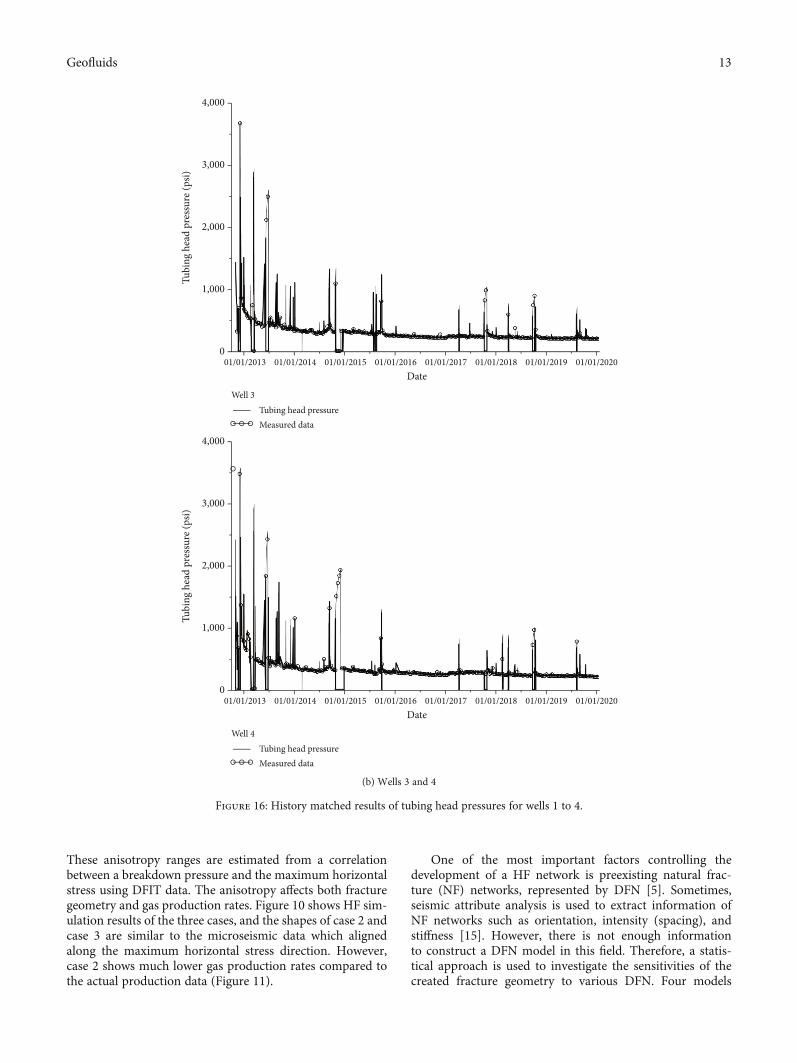
(b) Wells 3 and 4

Figure 16: History matched results of tubing head pressures for wells 1 to 4.

13Geofluids

001/01/2013 01/01/2014 01/01/2015 01/01/2016

Date01/01/2017 01/01/2018 01/01/2019 01/01/2020

200,000

400,000

Gas

pro

duct

ion

rate

(m3 /d

)600,000

800,000

1,000,000

Well 1Gas production rateMeasured data

001/01/2013 01/01/2014 01/01/2015 01/01/2016

Date01/01/2017 01/01/2018 01/01/2019 01/01/2020

200,000

400,000

Gas

pro

duct

ion

rate

(m3 /d

)

600,000

800,000

1,000,000

Well 2Gas production rateMeasured data

/01/2013 01/01/2014 01/01/2015 01/01/2016Date

01/01/2017 01/01/2018 01/01/2019 01/01/

Well 1Gas production rateMeasured data

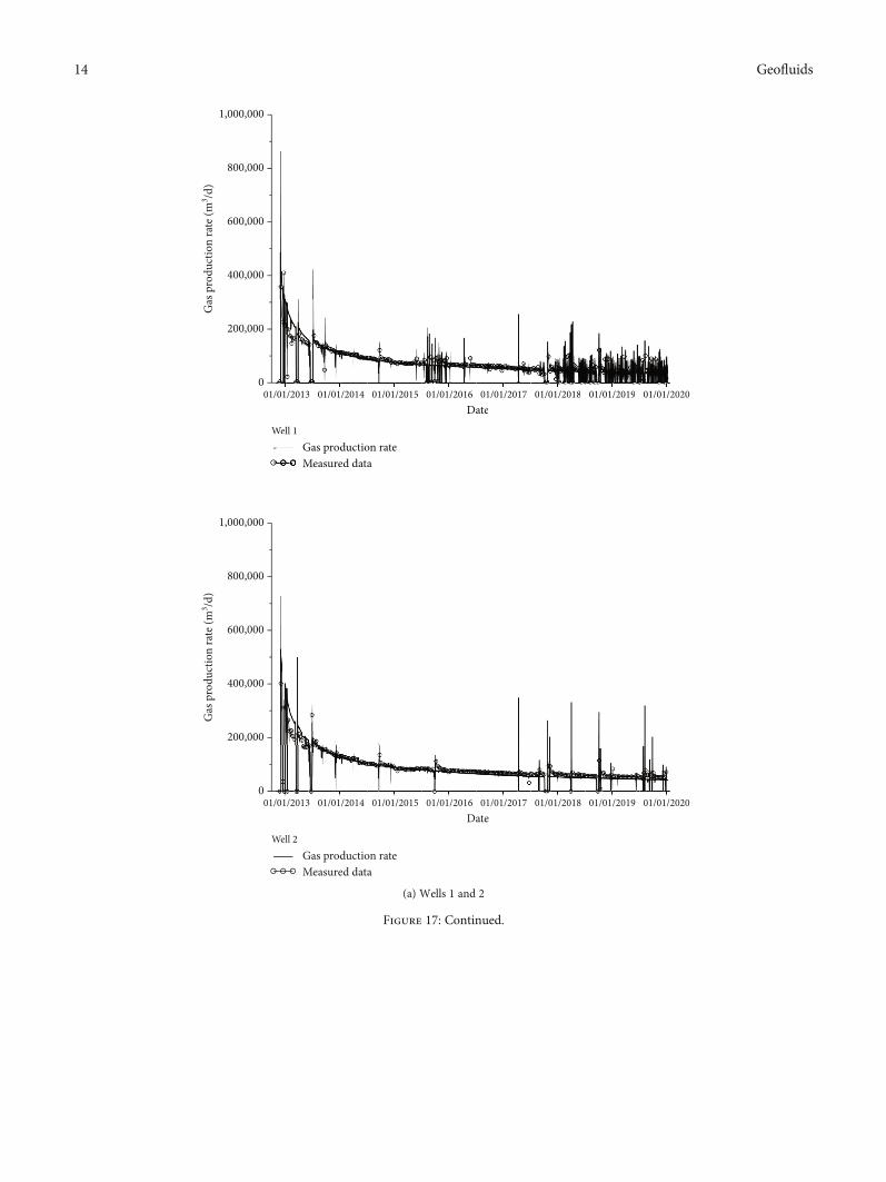
(a) Wells 1 and 2

Figure 17: Continued.

14 Geofluids

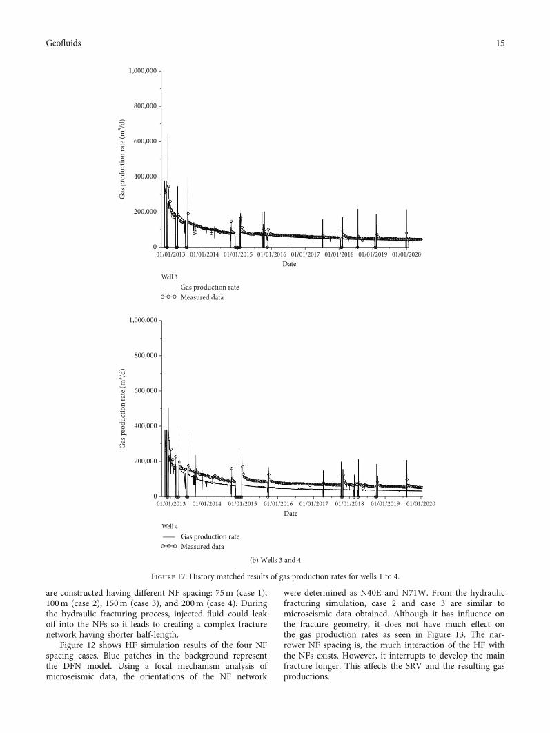
are constructed having different NF spacing: 75m (case 1),100m (case 2), 150m (case 3), and 200m (case 4). Duringthe hydraulic fracturing process, injected fluid could leakoff into the NFs so it leads to creating a complex fracturenetwork having shorter half-length.

Figure 12 shows HF simulation results of the four NFspacing cases. Blue patches in the background representthe DFN model. Using a focal mechanism analysis ofmicroseismic data, the orientations of the NF network

were determined as N40E and N71W. From the hydraulicfracturing simulation, case 2 and case 3 are similar tomicroseismic data obtained. Although it has influence onthe fracture geometry, it does not have much effect onthe gas production rates as seen in Figure 13. The nar-rower NF spacing is, the much interaction of the HF withthe NFs exists. However, it interrupts to develop the mainfracture longer. This affects the SRV and the resulting gasproductions.

001/01/2013 01/01/2014 01/01/2015 01/01/2016

Date01/01/2017 01/01/2018 01/01/2019 01/01/2020

200,000

400,000

Gas

pro

duct

ion

rate

(m3 /d

)

600,000

800,000

1,000,000

Well 3Gas production rateMeasured data

001/01/2013 01/01/2014 01/01/2015 01/01/2016

Date01/01/2017 01/01/2018 01/01/2019 01/01/2020

200,000

400,000

Gas

pro

duct

ion

rate

(m3 /d

)

600,000

800,000

1,000,000

Well 4Gas production rateMeasured data

(b) Wells 3 and 4

Figure 17: History matched results of gas production rates for wells 1 to 4.

15Geofluids

3.4. Production Estimation. The HF simulation of a pad wasconducted using the calibrated MEM parameters of the sin-gle well. For NF spacing, both cases 2 and 3 were tested,and case 3 was appropriate for the whole pad. Figure 14shows the fracture simulation results of the pad. It is foundthat overall created fracture geometry is similar to that ofmicroseismic data, so the MEM is updated using the calibra-tion factors.

Finally, production estimation of the pad is performed tovalidate the integrated workflow in the shale gas reservoir. Anunstructured grid for the fracture network is generated con-sisting of 15 layers with 3 million cells. In addition to the res-ervoir grid, a fluid model, relative permeability, and pressure-dependent permeability are put into the reservoir simulator.Figure 15 represents pressure-dependent permeability multi-pliers of each region. As the reservoir pressure is depleting,permeability of each region is decreasing. Proppant place-ment helps to support against fracture closure, so permeabil-ity is maintained during the depletion.

About seven years, gas production data of the four wellsare used for comparison and tubing head pressures of eachwell are utilized as a constraint. Figures 16 and 17 presentsimulated results of tubing head pressures and gas produc-tions, respectively. The black dots indicate field measureddata, and solid lines represent simulation results. Althoughfracture designs of four wells are slightly different, themodel could estimate seven-year production history of thepad reasonably due to proper use of parameters calibrated.The global error shows 8% for the whole pad.

Therefore, the integrated approach proposed in thisstudy will be useful to predict reliable future gas productionsand to optimize HF design or operation conditions in thefield. This study was conducted based on a deterministic sin-gle mechanical earth model, but stochastic approaches couldalso be taken to evaluate the uncertainties of rock mechani-cal, natural fracture, and stress-related parameters.

4. Conclusions

In this research, an integrated workflow is suggested and val-idated with the actual field data. It consists of building amechanical earth model, calibrating the model, and estimat-ing gas productions. The MEM is constructed using seismicattribute and drilling and DFIT analysis results. Based onthe model, hydraulic fracture propagation of a single well ina pad is simulated and compared with microseismic data.In addition, gas production rates are compared for each ofuncertain parameters for selecting proper values.

From the DFIT analyses, pressure-dependent leakoffmechanism is dominant in this field and leakoff multipliersare calculated. High leakoff coefficient causes most of injectedfluid coming into the matrix and natural fracture. Therefore,it leads to generating shorter fracture half-length and less gasproductions. The horizontal stress anisotropy affects theshape of the created fracture network. As the anisotropyincreases, a planar-type fracture network is generated andthe opposite case results in a complex-type fracture network.The natural fracture spacing is related to the interaction of

the HF with NFs. However, it does not have much impacton the gas production rates.

The MEM is updated using calibrated parameters from asingle-well case, and the pad scale simulation is conducted tovalidate the model parameters selected. Simulation results ofthe four wells, which have slightly different fracture designs,are well matched with microseismic data. After the hydraulicfractures are modelled and calibrated, an unstructured gridthat contains fracture geometry and proppant distributionis built. Production estimations of the pad are comparedwith the seven-year production history, and their resultsare reasonably similar to the actual data (global error: 8%)due to proper use of geomechanical parameters calibrated.

The developed workflow has some availability for furtherstudies. It will be useful to predict future gas productions andapplicable to other shale gas reservoirs. It could be also usedto decide an optimal HF design using the calibrated MEM.

Nomenclature

Cdp: PDL coefficient of leakoff (1/kPaÞCo: Original matrix leakoff coefficient (m/√min)Cp: Altered leakoff coefficient (m/√min)E: Young’s modulus (1/GPa)FL: Linear flow time function (dimensionless)FR: Radial flow time function (dimensionless)g: Average decline rate function (dimensionless)g0: Initial decline rate (dimensionless)G: G-function (dimensionless)h: Net pay thickness (m)k: Permeability (md)mL: Slope of data on pseudolinear flow graph (MPa)mR: Slope of data on pseudoradial flow graph (MPa)pi: Initial reservoir pressure (MPa)pr: Reservoir pressure (MPa)pw: Falloff pressure (MPa)Δp: Net pressure (MPa)t: Actual time (minutes)tc: Closure time (minutes)tp: Pumping time (minutes)ΔtD: Dimensionless shut-in time (dimensionless)Vp: p-wave velocity (km/s)Vs: s-wave velocity (km/s)α: Biot constant (dimensionless)μ: Viscosity (cp)ν: Poisson’s ratio (dimensionless)ρ: Density (kg/m3)σc: Closure stress (MPa)σh: Minimum horizontal stress (MPa)σH : Maximum horizontal stress (MPa)σt: Tectonic stress (MPa)σv: Vertical stress (MPa).

Data Availability

The data used to support the finding of this study areincluded within the article.

16 Geofluids

Conflicts of Interest

The authors declare that there is no conflict of interestregarding the publication of this paper.

Acknowledgments

The authors would like to thank Korea Gas Corporation andKOGAS Canada Limited for the permission to publish thisarticle. The corresponding author also likes to thank MOTIEprojects (20204010600250, 20162010201980) and the Insti-tute of Engineering Research at Seoul National University,Korea.

References

[1] S. Nejadi, J. Y. W. Leung, J. J. Trivedi, and C. Virues, “Inte-grated characterization of hydraulically fractured shale-gasreservoirs-production history matching,” SPE Reservoir Evalu-ation & Engineering, vol. 18, no. 4, pp. 481–494, 2015.

[2] R. Yu, Y. Bian, Y. Qi et al., “Qualitative modeling of multi-stage fractured horizontal well productivity in shale gas reser-voir,” Energy Exploration & Exploitation, vol. 35, no. 4,pp. 516–527, 2017.

[3] H. Chang and D. Zhang, “History matching of stimulated res-ervoir volume of shale-gas reservoirs using an iterative ensem-ble smoother,” SPE Journal, vol. 23, no. 2, pp. 346–366, 2018.

[4] F. Ajisafe, D. Shan, F. Alimahomed, S. Lati, and E. Ejofodomi,“An integrated workflow for completion and stimulationdesign optimization in the Avalon Shale, Permian Basin,”SPE 185672 presented at SPE Western Regional Meeting, Soci-ety of Petroleum Engineers, 2017, Bakersfield, CA, USA, 2017.

[5] C. Cipolla, X. Weng, M. Mack et al., “Integrating microseismicmapping and complex fracture modeling to characterize frac-ture complexity,” in SPE 140185 presented at SPE HydraulicFracturing Technology Conference and Exhibition, The Wood-lands, TX, USA, 2011.

[6] G. Izadi, R. Guises, C. Barton et al., “Advanced integrated sub-surface 3D reservoir model for multistage full-physic hydraulicfracturing simulation,” in IPTC 20064 presented at Interna-tional Petroleum Technology Conference, Dhahran, Saudi Ara-bia, 2020.

[7] T. Lee, D. Park, C. Shin, D. Jeong, and J. Choe, “Efficient pro-duction estimation for a hydraulic fractured well consideringfracture closure and proppant placement effects,” EnergyExploration & Exploitation, vol. 34, no. 4, pp. 643–658, 2016.

[8] P. Pankaj, P. Shukla, P. Kavousi, and T. Carr, “Determiningoptimal well spacing in the Marcellus Shale: a case study usingan integrated workflow,” SPE 191862 presented at SPE Argen-tina Exploration and Production of Unconventioanl ResourcesSymposium, Society of Petroleum Engineers, 2018, San Anto-nio, Neuquen, Argentina, 2018.

[9] K. Nolte, J. Maniere, and K. Owens, “After-closure analysis offracture calibration tests,” in SPE 38676 presented at SPEAnnual Technical Conference and Exhibition, San Antonio,TX, USA, 1997.

[10] K. Nolte, “Determination of fracture parameters from fractur-ing pressure decline,” in SPE 8341 presented at SPE AnnualTechnical Conference and Exhibition, Las Vegas, NV, USA,1979.

[11] D. P. Craig, R. D. Barree, N. R. Warpinski, and T. A. Blasin-game, “Fracture closure stress: reexamining field and labora-tory experiments of fracture closure using moderninterpretation methodologies,” in SPE 187038 presented atSPE Annual Technical Conference and Exhibition, San Anto-nio, TX, USA, 2017.

[12] X. Weng, O. Kresse, D. Chuprakov, C. Cohen, R. Prioul, andU. Ganguly, “Applying complex fracture model and integratedworkflow in unconventional reservoirs,” Journal of PetroleumScience and Engineering, vol. 124, pp. 468–483, 2014.

[13] R. D. Barree, J. Miskimins, and J. Gilbert, “Diagnostic fractureinjection tests: commonmistakes, misfires, and misdiagnoses,”SPE Production & Operations, vol. 30, no. 2, pp. 84–98, 2015.

[14] R. Plumb, S. Edward, G. Pidcock, D. Lee, and B. Stacey, “Themechanical earth model concept and its application to high-risk well construction projects,” in SPE 59128 presented atIADC/SPE Drilling Conference, 2000New Orleans, LA, USA.

[15] Y. Cho, R. L. Gibson Jr., J. Lee, and C. Shin, “Linear-slip dis-crete fracture network model and multiscale seismic wave sim-ulation,” Journal of Applied Geophysics, vol. 160, pp. 140–152,2017.

17Geofluids