State of Ohio Wetland Ecology GroupEnvironmental Protection Agency Division of Surface Water

INTEGRATED WETLAND ASSESSMENT PROGRAM.Part 6: Standardized Monitoring Protocols and Performance Standards

for Wetland Creation, Enhancement and Restoration, Version 1.0

Ohio EPA Technical Report WET/2004-6

Bob Taft, Governor Joseph P. Koncelik, DirectorState of Ohio Environmental Protection Agency

P.O. Box 1049, Lazarus Government Center, 122 S. Front Street, Columbus, Ohio 43216-1049 ——————————————————————————————————————

ii

Appropriate Citation:

Mack, John J, M. Siobhan Fennessy, Mick Micacchion and Deni Porej. 2004. Standardized monitoringprotocols, data analysis and reporting requirements for mitigation wetlands in Ohio, v. 1.0. Ohio EPATechnical Report WET/2004-6. Ohio Environmental Protection Agency, Division of Surface Water,Wetland Ecology Group, Columbus, Ohio.

This entire document can be downloaded from the website of the Ohio EPA, Division of Surface Water:

http://www.epa.state.oh.us/dsw/wetlands/WetlandEcologySection.html

iii

ACKNOWLEDGMENTS

This report would not have been possible without the encouragement and support of Richard Sumner andSue Elston (U.S. EPA) and the input and reviews of Mick Micacchion, Randy Bournique and the staff ofthe 401 Water Quality Certification Section (Jeff Boyles, Pete Clingan, Art Coleman, Laura Fay, DanOsterfeld, Mike Smith) This project was funded in part by Wetland Program Development Grant No.CD975350, Region 5, U.S Environmental Protection Agency.

iv

TABLE OF CONTENTS

ACKNOWLEDGMENTS . . . . . . . . . . . . . . . . . . . . . . . . . . . . . . . . . . . . . . . . . . . . . . . . . . . . . . . . . . . . . ii

TABLE OF CONTENTS . . . . . . . . . . . . . . . . . . . . . . . . . . . . . . . . . . . . . . . . . . . . . . . . . . . . . . . . . . . . . . iii

LIST OF TABLES . . . . . . . . . . . . . . . . . . . . . . . . . . . . . . . . . . . . . . . . . . . . . . . . . . . . . . . . . . . . . . . . . . viii

LIST OF FIGURES . . . . . . . . . . . . . . . . . . . . . . . . . . . . . . . . . . . . . . . . . . . . . . . . . . . . . . . . . . . . . . . . . . ix

ABSTRACT . . . . . . . . . . . . . . . . . . . . . . . . . . . . . . . . . . . . . . . . . . . . . . . . . . . . . . . . . . . . . . . . . . . . . . . . xi

1.0 BACKGROUND . . . . . . . . . . . . . . . . . . . . . . . . . . . . . . . . . . . . . . . . . . . . . . . . . . . . . . . . . . . . . . . . . 1

1.1 Introduction . . . . . . . . . . . . . . . . . . . . . . . . . . . . . . . . . . . . . . . . . . . . . . . . . . . . . . . . . . . . . . 11.2 Condition-based approach to functional replacement . . . . . . . . . . . . . . . . . . . . . . . . . . . . . . 11.3 Investigating Structure and Function of Natural and Mitigation Wetlands . . . . . . . . . . . . . . 31.4 Mitigation Performance and Monitoring . . . . . . . . . . . . . . . . . . . . . . . . . . . . . . . . . . . . . . . . 5

1.4.1 Size (No Net Loss of Wetland Acreage) . . . . . . . . . . . . . . . . . . . . . . . . . . . . . . . . 61.4.2 Consolidation and Morphometry . . . . . . . . . . . . . . . . . . . . . . . . . . . . . . . . . . . . . . 61.4.3 Hydrology . . . . . . . . . . . . . . . . . . . . . . . . . . . . . . . . . . . . . . . . . . . . . . . . . . . . . . . 61.4.4 Biogeochemistry . . . . . . . . . . . . . . . . . . . . . . . . . . . . . . . . . . . . . . . . . . . . . . . . . . 61.4.5 Basic Vegetation Establishment . . . . . . . . . . . . . . . . . . . . . . . . . . . . . . . . . . . . . . 61.4.6 Woody Vegetation Establishment . . . . . . . . . . . . . . . . . . . . . . . . . . . . . . . . . . . . . 71.4.7 Measures of Ecologic Condition . . . . . . . . . . . . . . . . . . . . . . . . . . . . . . . . . . . . . . 7

1.4.7.1 Vegetation Index of Biotic Integrity (VIBI) . . . . . . . . . . . . . . . . . . . . . 71.4.7.2 Amphibian Index of Biotic Integrity (AmphIBI) . . . . . . . . . . . . . . . . . . 71.4.7.3 Other Measures of Condition, Function, or Value . . . . . . . . . . . . . . . . 7

1.5 Using the Standardized Mitigation Performance Standards and Monitoring Protocols . . . . 8

2.0 PERFORMANCE STANDARDS FOR WETLAND CREATION, RESTORATION, ANDENHANCEMENT . . . . . . . . . . . . . . . . . . . . . . . . . . . . . . . . . . . . . . . . . . . . . . . . . . . . . . . . . . . . 8

2.1 General standards . . . . . . . . . . . . . . . . . . . . . . . . . . . . . . . . . . . . . . . . . . . . . . . . . . . . . . . . . . 82.1.1 Acreage . . . . . . . . . . . . . . . . . . . . . . . . . . . . . . . . . . . . . . . . . . . . . . . . . . . . . . . . . . 82.1.2 Basin morphometry . . . . . . . . . . . . . . . . . . . . . . . . . . . . . . . . . . . . . . . . . . . . . . . . 82.1.3 Perimeter:Area ratio . . . . . . . . . . . . . . . . . . . . . . . . . . . . . . . . . . . . . . . . . . . . . . . . 92.1.4 Characteristic hydrologic regime . . . . . . . . . . . . . . . . . . . . . . . . . . . . . . . . . . . . . . 9

2.2 Ecological standards - Vegetation . . . . . . . . . . . . . . . . . . . . . . . . . . . . . . . . . . . . . . . . . . . . . 92.2.1 Unvegetated open water . . . . . . . . . . . . . . . . . . . . . . . . . . . . . . . . . . . . . . . . . . . . . 92.2.2 Native wetland species establishment . . . . . . . . . . . . . . . . . . . . . . . . . . . . . . . . . . 92.2.3 Invasive species . . . . . . . . . . . . . . . . . . . . . . . . . . . . . . . . . . . . . . . . . . . . . . . . . . . 92.2.4 Ecological condition . . . . . . . . . . . . . . . . . . . . . . . . . . . . . . . . . . . . . . . . . . . . . . . 9

2.2.4.1 Vegetation IBI score . . . . . . . . . . . . . . . . . . . . . . . . . . . . . . . . . . . . . . . 92.2.4.2 Intermediate community goals . . . . . . . . . . . . . . . . . . . . . . . . . . . . . . . . 9

v

2.2.5 Establishment of woody vegetation . . . . . . . . . . . . . . . . . . . . . . . . . . . . . . . . . . . . 92.2.5.1 Shrub swamp . . . . . . . . . . . . . . . . . . . . . . . . . . . . . . . . . . . . . . . . . . . . . 92.2.5.2 Swamp forest . . . . . . . . . . . . . . . . . . . . . . . . . . . . . . . . . . . . . . . . . . . . 10

2.3 Characteristic amphibian community . . . . . . . . . . . . . . . . . . . . . . . . . . . . . . . . . . . . . . . . . 102.4 Ecologic standards - Other taxa groups . . . . . . . . . . . . . . . . . . . . . . . . . . . . . . . . . . . . . . . . 102.5 Characteristic soil chemistry processes . . . . . . . . . . . . . . . . . . . . . . . . . . . . . . . . . . . . . . . . 102.6 Ecological services (functions and values) . . . . . . . . . . . . . . . . . . . . . . . . . . . . . . . . . . . . . 10

3.0 MONITORING EVENTS AND MONITORING PERIOD . . . . . . . . . . . . . . . . . . . . . . . . . . . . . . . 10

4.0 STANDARDIZED MONITORING PROTOCOLS TO DETERMINE CONFORMANCE WITHPERFORMANCE STANDARDS . . . . . . . . . . . . . . . . . . . . . . . . . . . . . . . . . . . . . . . . . . . . . . . 11

4.1 Monitoring for general standards . . . . . . . . . . . . . . . . . . . . . . . . . . . . . . . . . . . . . . . . . . . . . 114.1.1 Actual Acreage . . . . . . . . . . . . . . . . . . . . . . . . . . . . . . . . . . . . . . . . . . . . . . . . . . 114.1.2 Basin morphometry . . . . . . . . . . . . . . . . . . . . . . . . . . . . . . . . . . . . . . . . . . . . . . . 124.1.3 Perimeter:Area ratio . . . . . . . . . . . . . . . . . . . . . . . . . . . . . . . . . . . . . . . . . . . . . . . 124.1.4 Hydrologic regime . . . . . . . . . . . . . . . . . . . . . . . . . . . . . . . . . . . . . . . . . . . . . . . . 12

4.2 Monitoring for ecological standards - Vegetation . . . . . . . . . . . . . . . . . . . . . . . . . . . . . . . . 134.2.1 Unvegetated open water . . . . . . . . . . . . . . . . . . . . . . . . . . . . . . . . . . . . . . . . . . . . 134.2.2 Native perennial hydrophytes . . . . . . . . . . . . . . . . . . . . . . . . . . . . . . . . . . . . . . 134.2.3 Invasive species . . . . . . . . . . . . . . . . . . . . . . . . . . . . . . . . . . . . . . . . . . . . . . . . . . 134.2.4 Vegetation IBI . . . . . . . . . . . . . . . . . . . . . . . . . . . . . . . . . . . . . . . . . . . . . . . . . . . 134.2.5 Woody species establishment . . . . . . . . . . . . . . . . . . . . . . . . . . . . . . . . . . . . . . . . 14

4.2.6.1 Basic Vegetation Survey Design for Single, Small, RelativelyHomogenous Wetlands . . . . . . . . . . . . . . . . . . . . . . . . . . . . . . . . . . . . 14

4.2.6.2 Random Vegetation Survey Design for Mitigation Banks and LargerIndividual Mitigations . . . . . . . . . . . . . . . . . . . . . . . . . . . . . . . . . . . . . 14

4.3 Monitoring for ecological standards - Amphibians . . . . . . . . . . . . . . . . . . . . . . . . . . . . . . . 154.4 Monitoring for other taxa groups . . . . . . . . . . . . . . . . . . . . . . . . . . . . . . . . . . . . . . . . . . . . . 16

4.4.1 Wetland Bird Sampling . . . . . . . . . . . . . . . . . . . . . . . . . . . . . . . . . . . . . . . . . . . . 164.4.2 Macroinvertebrates . . . . . . . . . . . . . . . . . . . . . . . . . . . . . . . . . . . . . . . . . . . . . . . 16

4.5 Characteristic biogeochemistry . . . . . . . . . . . . . . . . . . . . . . . . . . . . . . . . . . . . . . . . . . . . . . 174.5.1 Soil sampling . . . . . . . . . . . . . . . . . . . . . . . . . . . . . . . . . . . . . . . . . . . . . . . . . . . . 174.5.2 Water sampling . . . . . . . . . . . . . . . . . . . . . . . . . . . . . . . . . . . . . . . . . . . . . . . . . . 17

4.6 Monitoring for Ecological Services or Specific Functions . . . . . . . . . . . . . . . . . . . . . . . . . 17

5.0 GENERAL DATA SUMMARY, ANALYSIS AND PRESENTATION . . . . . . . . . . . . . . . . 17

5.1 Introduction . . . . . . . . . . . . . . . . . . . . . . . . . . . . . . . . . . . . . . . . . . . . . . . . . . . . . . . . . . 175.2 General Data Analysis and Presentation . . . . . . . . . . . . . . . . . . . . . . . . . . . . . . . . . . . . 18

5.2.1 Descriptive and Graphical Methods . . . . . . . . . . . . . . . . . . . . . . . . . . . . . . . . . 185.2.2 Control charts, performance curves and regression analysis . . . . . . . . . . . . . . 185.2.3 Summary tables . . . . . . . . . . . . . . . . . . . . . . . . . . . . . . . . . . . . . . . . . . . . . . . . . 185.2.3 Analysis of Variance . . . . . . . . . . . . . . . . . . . . . . . . . . . . . . . . . . . . . . . . . . . . . 185.2.4 Multivariate methods . . . . . . . . . . . . . . . . . . . . . . . . . . . . . . . . . . . . . . . . . . . . 19

vi

6.0 ANALYSIS AND PRESENTATION OF MONITORING DATA TO DETERMINEPERFORMANCE . . . . . . . . . . . . . . . . . . . . . . . . . . . . . . . . . . . . . . . . . . . . . . . . . . . . . . . . . . . . 19

6.1 General Standards . . . . . . . . . . . . . . . . . . . . . . . . . . . . . . . . . . . . . . . . . . . . . . . . . . . . . 196.1.1 Acreage . . . . . . . . . . . . . . . . . . . . . . . . . . . . . . . . . . . . . . . . . . . . . . . . . . . . . . . 196.1.2 Basin Morphometry . . . . . . . . . . . . . . . . . . . . . . . . . . . . . . . . . . . . . . . . . . . . . 206.1.3 Perimeter:Area Ratio . . . . . . . . . . . . . . . . . . . . . . . . . . . . . . . . . . . . . . . . . . . . 206.1.4 Hydrologic Regime . . . . . . . . . . . . . . . . . . . . . . . . . . . . . . . . . . . . . . . . . . . . . . 21

6.1.4.1 Determining HGM class . . . . . . . . . . . . . . . . . . . . . . . . . . . . . . . . . . . 216.1.4.2 Evaluating quantitative hydrologic data . . . . . . . . . . . . . . . . . . . . . . . 21

6.2 Vegetation . . . . . . . . . . . . . . . . . . . . . . . . . . . . . . . . . . . . . . . . . . . . . . . . . . . . . . . . . . . 226.2.1 Unvegetated Open Water . . . . . . . . . . . . . . . . . . . . . . . . . . . . . . . . . . . . . . . . . 226.2.2 Native perennial hydrophytes . . . . . . . . . . . . . . . . . . . . . . . . . . . . . . . . . . . . . . 236.2.3 Invasive Species . . . . . . . . . . . . . . . . . . . . . . . . . . . . . . . . . . . . . . . . . . . . . . . . 236.2.4 Vegetation - Ecologic Standards . . . . . . . . . . . . . . . . . . . . . . . . . . . . . . . . . . . 246.2.5 Woody spp. Establishment . . . . . . . . . . . . . . . . . . . . . . . . . . . . . . . . . . . . . . . . 256.2.6 Data presentation for vegetation data . . . . . . . . . . . . . . . . . . . . . . . . . . . . . . . . 27

6.3 Amphibians - Ecologic Standards . . . . . . . . . . . . . . . . . . . . . . . . . . . . . . . . . . . . . . . . . 276.4 Other taxa groups - Ecologic Standards . . . . . . . . . . . . . . . . . . . . . . . . . . . . . . . . . . . . 286.5 Biogeochemical Standards . . . . . . . . . . . . . . . . . . . . . . . . . . . . . . . . . . . . . . . . . . . . . . . 286.6 Ecological Services . . . . . . . . . . . . . . . . . . . . . . . . . . . . . . . . . . . . . . . . . . . . . . . . . . . . 28

7.0 STANDARD MITIGATION MONITORING REPORT FORMAT . . . . . . . . . . . . . . . . . . . . . . . . 28

7.1. Executive Summary . . . . . . . . . . . . . . . . . . . . . . . . . . . . . . . . . . . . . . . . . . . . . . . . . . . . . . 297.2 Background information . . . . . . . . . . . . . . . . . . . . . . . . . . . . . . . . . . . . . . . . . . . . . . . . . . . 297.3 Methods - Monitoring Protocols and Performance Standards . . . . . . . . . . . . . . . . . . . . . . . 297.4 Results and Discussion . . . . . . . . . . . . . . . . . . . . . . . . . . . . . . . . . . . . . . . . . . . . . . . . . . . . 29

7.4.1 Size, Morphometry, Perimeter:Area Ratio . . . . . . . . . . . . . . . . . . . . . . . . . . . . 297.4.2 Hydrology . . . . . . . . . . . . . . . . . . . . . . . . . . . . . . . . . . . . . . . . . . . . . . . . . . . . . 307.4.3 Vegetation Data . . . . . . . . . . . . . . . . . . . . . . . . . . . . . . . . . . . . . . . . . . . . . . . . 307.4.4 Amphibian Data . . . . . . . . . . . . . . . . . . . . . . . . . . . . . . . . . . . . . . . . . . . . . . . . 307.4.5 Biogeochemistry Data . . . . . . . . . . . . . . . . . . . . . . . . . . . . . . . . . . . . . . . . . . . . 31

7.5 Conclusions . . . . . . . . . . . . . . . . . . . . . . . . . . . . . . . . . . . . . . . . . . . . . . . . . . . . . . . . . . . . . 317.6 Appendices - Paper . . . . . . . . . . . . . . . . . . . . . . . . . . . . . . . . . . . . . . . . . . . . . . . . . . . . . . . 317.7 Appendices - Electronic Submissions . . . . . . . . . . . . . . . . . . . . . . . . . . . . . . . . . . . . . . . . . 31

8.0 MITIGATION BANKS . . . . . . . . . . . . . . . . . . . . . . . . . . . . . . . . . . . . . . . . . . . . . . . . . . . . . . . . . . 31

8.1 Performance Standards and Monitoring Protocols at Mitigation Banks . . . . . . . . . . . . . . . 328.1.1 Acreage . . . . . . . . . . . . . . . . . . . . . . . . . . . . . . . . . . . . . . . . . . . . . . . . . . . . . . . . 328.1.2 Basin Morphometry . . . . . . . . . . . . . . . . . . . . . . . . . . . . . . . . . . . . . . . . . . . . . . . 328.1.3 Perimeter:Area Ratio . . . . . . . . . . . . . . . . . . . . . . . . . . . . . . . . . . . . . . . . . . . . . . 328.1.4 Hydrology . . . . . . . . . . . . . . . . . . . . . . . . . . . . . . . . . . . . . . . . . . . . . . . . . . . . . . 328.2.1 Unvegetated Open Water . . . . . . . . . . . . . . . . . . . . . . . . . . . . . . . . . . . . . . . . . . . 328.2.2 Perennial Native Hydrophytes . . . . . . . . . . . . . . . . . . . . . . . . . . . . . . . . . . . . . . . 33

vii

8.2.3 Invasive Species . . . . . . . . . . . . . . . . . . . . . . . . . . . . . . . . . . . . . . . . . . . . . . . . . . 338.2.4 Ecologic Condition: Vegetation IBI . . . . . . . . . . . . . . . . . . . . . . . . . . . . . . . . . . 338.2.5 Woody Species Establishment . . . . . . . . . . . . . . . . . . . . . . . . . . . . . . . . . . . . . . . 33

8.3 Ecologic Condition: Amphibian IBI . . . . . . . . . . . . . . . . . . . . . . . . . . . . . . . . . . . . . . . . . . 338.4 Biogeochemistry . . . . . . . . . . . . . . . . . . . . . . . . . . . . . . . . . . . . . . . . . . . . . . . . . . . . . . . . . 348.5 Other Measures of Condition or Function . . . . . . . . . . . . . . . . . . . . . . . . . . . . . . . . . . . . . . 348.6 In-Kind Replacement and Mitigation Banks . . . . . . . . . . . . . . . . . . . . . . . . . . . . . . . . . . . 348.7 Performance-Driven Credit Release Schedules . . . . . . . . . . . . . . . . . . . . . . . . . . . . . . . . . . 34

9.0 STANDARD CONDITIONS FOR SECTION CERTIFICATIONS AND PERMITS . . . . . . . . . . 34

10.0 LITERATURE CITED . . . . . . . . . . . . . . . . . . . . . . . . . . . . . . . . . . . . . . . . . . . . . . . . . . . . . . . . . . 39

viii

LIST OF TABLES

Table 1a. Hydrogeomorphic classes for wetland classification system for Ohio wetlands. . . . . . . . . . . 42Table 1b. Plant community modifiers for Wetland classification system for Ohio wetlands. . . . . . . . . 43Table 2a. Mean hydrological indicators by HGM class. . . . . . . . . . . . . . . . . . . . . . . . . . . . . . . . . . . . . 44Table 2b. Surface water levels for Lake Erie Coastal Marsh. . . . . . . . . . . . . . . . . . . . . . . . . . . . . . . . . 44Table 3. Ranges for Vegetation IBI scores for Category 2 and 3 Wetlands by HGM class, plant

community class, and ecoregion. . . . . . . . . . . . . . . . . . . . . . . . . . . . . . . . . . . . . . . . . . . . . . . . . 45Table 4. Regression equations and minimum slopes for performance curves . . . . . . . . . . . . . . . . . . . . 46Table 5. Performance standards for wetland soils . . . . . . . . . . . . . . . . . . . . . . . . . . . . . . . . . . . . . . . . . 47Table 6a. Conceptual 5 year schedule of monitoring activities . . . . . . . . . . . . . . . . . . . . . . . . . . . . . . . 50Table 6b. Conceptual 10 year schedule of monitoring activities . . . . . . . . . . . . . . . . . . . . . . . . . . . . . . . 50Table 7. Conceptual schedule of activities during monitoring event . . . . . . . . . . . . . . . . . . . . . . . . . . . 50Table 8. Summary of performance standards and the monitoring data used to determine conformance

with the standard. . . . . . . . . . . . . . . . . . . . . . . . . . . . . . . . . . . . . . . . . . . . . . . . . . . . . . . . . . . . . 51Table 9. Minimum hydrologic monitoring requirements. . . . . . . . . . . . . . . . . . . . . . . . . . . . . . . . . . . . 53Table 10. Summary of vegetation survey data for plot based vegetation sampling method. . . . . . . . . . 54Table 11. Analytical parameters and suggested methods for soil analysis. . . . . . . . . . . . . . . . . . . . . . . 55Table 12. Example of summary table for VIBI scores, metric values, and chemistry data. . . . . . . . . . . 56Table 13. Example of summary table for multiple sites . . . . . . . . . . . . . . . . . . . . . . . . . . . . . . . . . . . . . 57Table 14. Summary table for acreage, morphometry, and perimeter:area ratio . . . . . . . . . . . . . . . . . . . 58Table 15. Description of HGM classes . . . . . . . . . . . . . . . . . . . . . . . . . . . . . . . . . . . . . . . . . . . . . . . . . . 59Table 16. Example hydrologic data from automated shallow ground water level recorder . . . . . . . . . . 60Table 17. Average forestry statistics by species for forest and shrub wetlands . . . . . . . . . . . . . . . . . . . 61Table 18. Background information on wetland type, location, and amount for wetland mitigation . . . 67Table 19. Summary of applicable performance standards. . . . . . . . . . . . . . . . . . . . . . . . . . . . . . . . . . . . 68Table 20. Summary of applicable monitoring and data analysis requirements. . . . . . . . . . . . . . . . . . . 69Table 21. Generic credit release schedule for mitigation banks. . . . . . . . . . . . . . . . . . . . . . . . . . . . . . . 70

ix

LIST OF FIGURES

Figure 1. Ecoregions of Ohio, Indiana, and neighboring states. . . . . . . . . . . . . . . . . . . . . . . . . . . . . . . . 71Figure 2. Typical hydrological signatures for depressions . . . . . . . . . . . . . . . . . . . . . . . . . . . . . . . . . . . 72Figure 3. Hydrologic signature of an impoundment . . . . . . . . . . . . . . . . . . . . . . . . . . . . . . . . . . . . . . . . 73Figure 4. Hydrologic signature of a slope wetland. . . . . . . . . . . . . . . . . . . . . . . . . . . . . . . . . . . . . . . . . 73Figure 5. Hydrologic signature of riverine wetlands . . . . . . . . . . . . . . . . . . . . . . . . . . . . . . . . . . . . . . . 74Figure 6. Hydrologic signature Lake Erie Coastal Wetland. . . . . . . . . . . . . . . . . . . . . . . . . . . . . . . . . . 75Figure 7. Hydrologic signature of stormwater influenced wetlands . . . . . . . . . . . . . . . . . . . . . . . . . . . . 76Figure 8. Performance curves for Vegetation IBI score for DEPRESSIONAL wetlands . . . . . . . . . . . 77Figure 9. Performance curves for Vegetation IBI score for WET MEADOW wetlands . . . . . . . . . . . . 78Figure 10. Performance curves for Vegetation IBI score for FOREST SEEP wetlands . . . . . . . . . . . . 78Figure 11. Performance curves for Vegetation IBI score for RIVERINE HEADWATER wetlands . . . 79Figure 12. Performance curves for Vegetation IBI score for RIVERINE MAINSTEM wetlands . . . . . 80Figure 13. Performance curves for Vegetation IBI score for IMPOUNDMENT wetlands . . . . . . . . . . 81Figure 14. Performance curves for Vegetation IBI score for BOG wetlands . . . . . . . . . . . . . . . . . . . . . 82Figure 15. Performance curves for Vegetation IBI score for Lake Erie COASTAL wetlands . . . . . . . 83Figure 16. Hypothetical performance curves for tree and shrub establishment at 10, 30, and 100 years for

DEPRESSIONAL wetland FORESTS (“vernal pools”) . . . . . . . . . . . . . . . . . . . . . . . . . . . . . . 84Figure 17. Hypothetical performance curves for tree and shrub establishment at 10, 30, and 100 years for

DEPRESSIONAL wetland SHRUB SWAMPS (“vernal pools”). . . . . . . . . . . . . . . . . . . . . . . . 85Figure 18. Hypothetical performance curves for tree and shrub establishment at 10, 30, and 100 years for

DEPRESSIONAL (flats) wetland FORESTS (“wet woods”). . . . . . . . . . . . . . . . . . . . . . . . . . . 86Figure 19. Hypothetical performance curves for tree and shrub establishment at 10, 30, and 100 years for

RIVERINE MAINSTEM wetland FORESTS. . . . . . . . . . . . . . . . . . . . . . . . . . . . . . . . . . . . . . . 87Figure 20. Hypothetical performance curves for tree and shrub establishment at 10, 30, and 100 years for

RIVERINE MAINSTEM wetland SHRUB SWAMPS. . . . . . . . . . . . . . . . . . . . . . . . . . . . . . . . 88Figure 21. Hypothetical performance curves for tree and shrub establishment at 10, 30, and 100 years for

FOREST SEEPS (slope, swamp forests). . . . . . . . . . . . . . . . . . . . . . . . . . . . . . . . . . . . . . . . . . . 89Figure 22. Hypothetical performance curves for tree and shrub establishment at 10, 30, and 100 years for

WEAKLY OMBROTROPHIC BOGS (TALL SHRUB BOG, TAMARACK-HARDWOODBOG). . . . . . . . . . . . . . . . . . . . . . . . . . . . . . . . . . . . . . . . . . . . . . . . . . . . . . . . . . . . . . . . . . . . . . 90

Figure 23. Hypothetical performance curves for tree and shrub establishment at 10, 30, and 100 years forMODERATELY TO STRONGLY OMBROTROPHIC BOGS (LEATHERLEAF BOG,TAMARACK BOG). . . . . . . . . . . . . . . . . . . . . . . . . . . . . . . . . . . . . . . . . . . . . . . . . . . . . . . . . . 91

Figure 24. Performance curves for AMPHIBIAN IBI score . . . . . . . . . . . . . . . . . . . . . . . . . . . . . . . . . 92Figure 25. Typical placement of transects to determine side slopes . . . . . . . . . . . . . . . . . . . . . . . . . . . 93Figure 26. Maximum allowable slopes in order to meet 15:1 side slope requirement. . . . . . . . . . . . . . 93Figure 27. Scenarios for determining perimeter:area ratio performance standard. . . . . . . . . . . . . . . . . 94Figure 28. Mitigation wetland with a predominance of open water and little emergent vegetation . . . 95Figure 29. Mitigation wetland with open water and a predominance of emergent vegetation . . . . . . . . 95Figure 30. Standard (fixed or focused) 20m x 50m (2 x 5) vegetation sample plot . . . . . . . . . . . . . . . 96Figure 31. A typical mixed emergent marsh with shrub margins, emergent zones, and open water. . . . 97Figure 32. A wet meadow community located within a matrix of upland prairie and savannah. . . . . . 97Figure 33. A buttonbush swamp located within an upland forest matrix. . . . . . . . . . . . . . . . . . . . . . . . 97Figure 34. A swamp forest (“wet woods”) located within an upland forest matrix. . . . . . . . . . . . . . . . 98Figure 35. A swamp forest (“vernal pool”) located within an upland forest matrix. . . . . . . . . . . . . . . . 98

x

Figure 36. A high quality marsh with a localized areas of Phalaris arundinacea. . . . . . . . . . . . . . . . . 98Figure 37. A wetland comprised of two HGM classes. . . . . . . . . . . . . . . . . . . . . . . . . . . . . . . . . . . . . . 99Figure 38. A wetland comprised of two co-dominant plant communities. . . . . . . . . . . . . . . . . . . . . . . . 99Figure 39. 10m x 10m geospatially referenced grid at Chippewa Central Mitigation Bank. . . . . . . . . 100Figure 40. Map of random plots at Chippew Central Mitigation Bank. . . . . . . . . . . . . . . . . . . . . . . . . 101Figure 41. Funnel (activity) trap for amphibian and macroinvertebrate sampling. . . . . . . . . . . . . . . . 102Figure 42. Typical funnel trap placement. . . . . . . . . . . . . . . . . . . . . . . . . . . . . . . . . . . . . . . . . . . . . . . 102Figure 43. Sampling scheme used to collect soil samples at all wetlands. . . . . . . . . . . . . . . . . . . . . . . 103Figure 44. Performance curve scenarios for a 10 year monitoring period . . . . . . . . . . . . . . . . . . . . . . 104Figure 45. Example of detrended correspondence analysis with environmental joint plots. . . . . . . . . 105

1 Ohio Environmental Protection Agency, Division of Surface Water, Wetland Ecology Group,4675 Homer Ohio Lane, Groveport, Ohio 43125, john.mack@epa.state.oh.us, mick.micacchion@epa.state.oh.us.

2 Department of Biology, Kenyon College, Gambier, Ohio, fennessym@kenyon.edu

3 The Nature Conservancy, Ohio Chapter, Dublin, Ohio, dporej@tnc.org

xi

INTEGRATED WETLAND ASSESSMENT PROGRAM.PART 6: STANDARDIZED MONITORING PROTOCOLS AND PERFORMANCE STANDARDS

FOR WETLAND CREATION, ENHANCEMENT AND RESTORATION, VERSION 1.0

John J. Mack1

M. Siobhan Fennessy2

Mick Micacchion1

Deni Porej3

ABSTRACT

A condition-based approach to assessing functional replacement for wetland mitigation has been developedusing a reference wetland data set of natural wetlands that includes data from the major wetland types thatspan a gradient of human disturbance. From this data set wetland program tools were developed 1)multimetric biological indices (IBIs) and hydrological and biogeochemical indicators; 2) a rapid (condition-based) wetland assessment tool (Ohio Rapid Assessment Method for Wetlands); and 3) a wetlandclassification scheme based on landscape position and dominant vegetation that accounts for variability inecosystem processes (functions) and ecological services (values) of different types of natural wetlands.Ensuring functional replacement occurs in a several step process. First, as part of permit application, theHGM class and dominant plant community of the impacted wetland(s) are determined. This determinationaccounts for the ecosystem processes (functions) and ecological services (values) of different wetland typeswithout the necessity of developing a comprehensive list of those functions and values. Second, thecondition of the impacted wetland is assessed with the rapid condition tool (ORAM v. 5.0) or a wetland IBIproviding a measure of "functional capacity." Third, the size of the wetland to be impacted is determined andappropriate mitigation ratios are applied. Fourth, any residual moderate to high functions or values theimpacted wetland(s) may still be providing, despite moderate to severe degradation, are evaluated usingchecklist with a narrative discussion. Finally, requirements for mitigation are specified in the permit. If thereis 1) replacement by size of the impacted wetland, 2) replacement of the type of wetland impacted, 3) andreplacement of the quality of the impacted wetland as measured by quantitative, condition-based ecologicalperformance targets, then there is very strong assurance that functional replacement is occurring since therewas “no net loss” of wetland acreage, a mitigation wetland of same HGM class and dominant plantcommunity was created with functions and ecological services equivalent to the impacted wetland, and amitigation wetland was created of equivalent “quality” as measured by biological (e.g. IBIs), hydrological,and biogeochemical indicators (and therefore of equivalent functional performance). Fundamentally, theabove approach is strongly data-driven and it follows then that meaningful and adequate mitigationmonitoring is absolutely necessary to determine whether the mitigation wetland has "succeeded" or "failed."Performance standards, quantitative monitoring, and data analysis techniques were developed for wetlandsize, basin morphometry, perimeter:area ratio, hydrologic regime, basic vegetation establishment, woodyspecies establishment (successional trends), soil chemistry, and wetland IBIs.

1

1.0 BACKGROUND

1.1 IntroductionCompensatory mitigation is one of the key

components of state and federal wetlandregulatory programs. It is a fundamental premise(assumption) that unavoidable, unminimizableimpacts causing loss of wetland acreage andfunction can be mitigated for by creating,enhancing or restoring wetlands elsewhere (onsite, in the same watershed, in the state, at awetland bank, etc.). There continues to be muchdebate, both scientifically and from a policyperspective whether this assumption is valid at all,or only valid for certain types and classes ofwetlands (e.g. Fennessy and Roehrs 1997; Mitschet al. 1998; Bedford 1999; Bedford 1996; NRC2001).

An intensive review and assessment ofwetland creation projects was recently publishedby the Committee on Mitigating Wetland Lossesconducted by the National Academy of SciencesNational Research Council (NRC 2001). Thecommittee concluded that “...the goal of no netloss of wetlands is not being met for wetlandfunctions by the mitigation program, despiteprogress in the last 20 years” (NRC 2001).Documenting mitigation wetland performance (orlack thereof) is a critical piece of information forimplementing a wetland regulatory program inorder to 1) evaluate programmatic success, 2)initiate changes in permit requirements or the useof current approval criteria if it is determined thatperformance and functional replacement are notoccurring, and 3) begin to address the largerissues of landscape level effects of constructingwetlands that may or may not have been prevalenthydrogeomorphically or vegetatively in aparticular region (Bedford 1996). Thefundamental issue then is how to obtain functionalreplacement of the impacted wetland and how tomeasure if such replacement has occurred.

1.2 Condition-based approach to functionalreplacement

The overall goal of the federal CleanWater Act is to maintain and restore the physical,chemical and biological integrity of the nation’swaters, with wetlands being a type of “water”along with streams and lakes. In streammonitoring programs, the dominant approach hasbeen to assess stream condition (integrity) usingintegrative biological measures (like IBIs). Theidea of talking about and assessing particularstream “functions” is a largely foreign concept,e.g. discussions of the “fishery” function ofstreams or the “pollutant dilution” of function ofstreams do not occur; rather, streams areconsidered and assessed as ecosystems. Thevarious ecosystem processes (functions) thatoccur in different types of streams are usually notdirectly measured but the level of functioning isinferred from integrative biological measures.

The terms “function” and “value” havebecome embedded in the language of wetlandprotection and assessment despite the fact that theClean Water Act goal is maintenance andrestoration of the chemical, physical andbiological integrity (i.e. condition) of wetlands.Thinking of wetland’s in terms ofcompartmentalized functions and values probablydeveloped, at least in part, as a heuristic approachin explaining to the public why wetland protectionand restoration is important.

It is difficult and time consuming toseparately quantify the functions of each wetlandpre- and post- impact in the context of aregulatory permit program. This function byfunction approach may ultimately explain thelimited extent that such approaches have beenadopted. In contrast, an approach that usescondition-based wetland assessment tools (e.g. anIndex of Biotic Integrity or IBI) derived from areference wetland data set is highly suited todetermining if functional replacement hasoccurred, and avoids the detailed specification of

2

functions for each permitted impact.4 The goal ofan IBI is to measure the ecological integrity(condition) of the wetland, with integrity beingdefined as deviation or lack thereof from regionalreference (least impacted) conditions. An IBItypically measures "structural" attributes of thebiological community and makes the assumptionthat if structural condition is good (or excellent ordegraded) then the functional processes thatsupport these structures are also operating at good(or excellent or degraded) levels (Stevenson andHauer 2002). Other data (chemical, physical andlandscape) are also collected but only biologicalattributes are included in the IBI. By keepingbiological information separate from physical,chemical or landscape information, it is easier toevaluate causal mechanisms and IBIs are arguablymore transparent and easier to explain thanmethods which incorporate different types of datainto untested logic models. The IBI approach hasa proven record of being able to measurerestoration and improvement of other aquaticresources like streams, lakes, and reservoirs.

A condition-based approach to functionalreplacement has, as its foundation, a referencewetland data set of natural wetlands that includesdata from the major wetland types and fromwetlands that span a gradient of humandisturbance.5 From this data set several wetland

program tools are developed 1) multimetricbiological indices (IBIs) and hydrological andbiogeochemical indicators; 2) a rapid (condition-based) wetland assessment tool calibrated usingthe IBIs (Ohio Rapid Assessment Method forWetlands); and 3) a wetland classification schemebased on landscape position and dominantvegetation that accounts for variability inecosystem processes (functions) and ecologicalservices (values) of different types of naturalwetlands (Mack 2001; Micacchion 2004; Knapp2004; Fennessy et al. 2004; Mack 2004a, b, c).

In the context of a permit application,functional replacement of the impacted wetland isa several step process. First, as part of permitapplication, the HGM class and dominant plantcommunity of the impacted wetland(s) must bedetermined. Specifying the type of wetland willaccount for different ecosystem processes(functions) and ecological services (values) ofdifferent wetland types without the necessity ofdeveloping a comprehensive list of thosefunctions and values. Second, the condition of theimpacted wetland is assessed with the rapidcondition tool (ORAM v. 5.0) or a wetland IBI.This provides a measure of "functional capacity"since "good" condition equates to "good"

4 Resident biological communities inhabit wetlands continuously or for significantportions of their life cycles, e.g. breeding or larvalstages, and are integrators of the prevailing and pastchemical, physical and biological history of thewetland (Ohio EPA 1988).

5 The HGM approach, as typicallydeveloped and practiced, does this by taking afunction by function approach (although Smith et al.(1995) state that “ecological integrity” is super-function at top of nested functional processhierarchy). In the HGM approach simple logicmodels (Smith et al. 1995, Brinson 1993) aredeveloped to infer functional performance. Typically

data from flora and faunal communities, water andsoil chemistry, land use information, etc. is collectedfrom wetland and this information is included inuntested logic models which, when summed, producea functional capacity index score. Scores and modelsare developed and calibrated using regional“reference standard” data sets. Reference standardsites are generally best remaining and/or leastimpacted examples of that type of wetland. Acommon misconception is that HGM actuallymeasures wetland “functions” directly; instead, HGMalmost always measures structural attributes (flora,fauna, physical features, etc.) of wetland and uses thecondition of these structural attributes in comparisonto reference standard conditions to infer functionalperformance. Biotic, abiotic, and sometimes evenlandscape level attributes are often included in thelogic models.

3

functioning. Third, the size of the wetland to beimpacted is determined. Mitigation ratios (OhioAdministrative Code 3745-1-54) are then used todetermine the amount of mitigation required.Fourth, any residual moderate to high functions orvalues the impacted wetland(s) may still beproviding, despite moderate to severe degradation,can be evaluated using a checklist approach witha narrative discussion (if necessary, a moredetailed quantification of residual functions canbe performed).6 Finally, requirements formitigation are specified in the permit. As part ofthe mitigation process mitigation occurs at ratiosspecified by rule with a minimum of 1:1replacement; replacement is “in-kind” with “in-kind” determined by the HGM class and dominantvegetation of the impacted wetland; andmitigation performance is determined byachievement of equivalent or greater “quality” asthe impacted wetland as measured by biological,hydrological, and biogeochemical indicatorsderived from reference wetland data sets. Theseindicators then become quantitative performancestandards and mitigation monitoring is thentailored to collect data necessary to determine ifthe standards have been met.

In conclusion, if there is 1) replacementby size of the impacted wetland, 2) replacement ofthe type of wetland impacted (same landscape

position and dominant plant community, 3) andreplacement of the quality of the impactedwetland as measured by quantitative, condition-based ecological performance targets, then thereis very strong assurance that functionalreplacement is occurring since there was “no netloss” of wetland acreage, a mitigation wetland ofsame HGM class and dominant plant communitywas created with functions and ecological servicesequivalent to the impact wetland, and a mitigationwetland was created of equivalent “quality” asmeasured by biological, hydrological, andbiogeochemical indicators (and therefore ofequiva len t func t iona l performance) .Fundamentally, the above approach is stronglydata-driven and it follows then that meaningfuland adequate mitigation monitoring is absolutelynecessary to determine whether the mitigationwetland has "succeeded" or "failed."

1.3 Investigating Structure and Function ofNatural and Mitigation Wetlands

The National Research Council (NRC2001) made multiple recommendations with thegoal of improving the success of wetlandmitigation 1) consider both the structure andfunction of wetland ecosystems, and therelationship between the them; 2) use referencewetlands as a model for the dynamics of createdor restored sites; 3) emphasize that hydrologicalvariability is important in the structure andfunction of mitigation wetlands; 4) require themeasurement of a broader range of functions formitigation projects; 5) broaden the science andtechnology of wetland restoration and creation toinclude sites that differ in degree of disturbanceand restoration effort; 6) construct self-sustainingmitigation wetlands; and 7) avoid the destructionof wetlands that are particularly hard to restore.7

6 To summarize the first four stepsdiscussed above: 1) classification by HGM class anddominant plant community provides assurance thatthe functions and values unique to that wetland typeare accounted for; 2) using a condition-basedassessment provides a measure of existing ecologicalcondition; “functional” performance is then inferredfrom level of condition, i.e. good condition = goodfunctional performance, excellent condition =excellent functional performance, poor condition =poor functional performance, etc.; and 3) evaluationof any residual functions or ecological services(values) provides safeguard against situation wheremoderate to severely degraded wetlands still have asingle “good” remaining function or value.

7 This last recommendation has beenincorporated into Ohio’s wetland water qualitystandards since 1998 where high quality or rare

4

In response to these recommendations, majorstudies of natural and mitigation wetlands in Ohiowere undertaken (Fennessy et al. 2004; Porej2003, 2004).

Ohio EPA undertook a comprehensiveinvestigation of the biota (structure) andbiogeochemical cycles (processes or functions) ofa population of natural and mitigation wetlandsusing a study design that incorporated the firstfour of the recommendations listed above(Fennessy et al. 2004). The objectives of thisstudy were four-fold: 1. To demonstrate the efficacy of using

floral and faunal community-basedindicators to assess the performance ofmitigation wetlands;

2. To investigate the linkages between floraand faunal community structuralattributes and ecosystem processes innatural and mitigation wetlands;

3. To investigate the biological and physicalcharacteristics, and biogeochemicalcycles of the wetlands in order to assessthe condition of mitigation sites ascompared to natural sites;

4. To identify simple, cost-effectivebiogeochemical indicators for use inmitigation monitoring. that can betranslated to performance standards.

Intensive fieldwork was conducted at natural andmitigation wetlands in order to collect data onvarious wetland ecosystem components (e.g.hydrology, soil, plant community composition andproductivity, macroinvertebrate and amphibiancommunity composition, decomposition, and

nutrient cycling). Where possible, this fieldworkwas supplemented by Ohio EPA's larger referencewetland data set. Fennessy et al. (2004) foundthat the mitigation wetlands, in terms of theirstructure and function, formed a separatepopulation from the natural wetlands, indicatingthe creation of a new subclass of wetlands on thelandscape. Major differences included deepersurface water at the mitigation sites; greater depthto ground water at the mitigation sites;substantially reduced soil nutrient pools atmitigation sites; significantly different movementof nutrients in terms of rates and quantitiesbetween natural and mitigation sites; reducednutrient availability that propagates throughoutthe mitigation systems and appears to set a limiton ecosystem development; and significantlydifferent compositions of plant, amphibian, andmacroinvertebrate communities.

Fennessy et al. (2004) concluded thatbiological and biogeochemical indicators wereeffective in their ability to reflect ecologicalcondition and measure mitigation wetlandperformance. Practical indicators in terms of cost,time, and information gained included soilchemical and physical characteristics especiallysoil organic carbon and soil nitrogen content andpercent solids in the soil or bulk density;hydrological characteristics including mean depthto ground water and percent time water is found inthe root zone (i.e. greater than -30cm) (ascompared to a natural reference ecosystem ofsimilar hydrogeomorphic class); and multimetricindices developed from natural reference wetlanddata sets.

In a second investigation, Porej (2004)developed predictive models based on landscape(%forest cover) and wetland characteristics(amount of shallow zones in wetland, presence ofpredatory fish) for Ohio amphibian species usingOhio EPA’s existing reference wetland data setand data collected from 48 mitigation sites. Porej(2004) found that the “amount of forest coverwetland types receive the highest level of regulatory

protection.

5

within the core zone [200m of the wetland] wasincluded in the most parsimonious models foroverall salamander diversity, and individualmodels for presence of spotted salamanders,Jefferson salamander complex (Ambystomajeffersonianum), smallmouth salamanders(Ambystoma texanum) and wood frogs” (Porej2004, p. 41). Land use beyond 200m (e.g.%forest, road density, etc.) was also important foroverall salamander diversity, red-spotted newts,tiger salamanders, and wood frogs (Porej 2004).

In addition to land use factors, Porej(2004) found that the absence of “littoral”shallows in the wetland and the presence ofpredacious fish species altered amphibianpopulations in natural and mitigation wetlands(Porej 2004). Overall amphibian diversity wassignificantly higher for wetlands with shallowsand without predacious fish than for wetlands thathad predacious fish, lacked shallows or had somecombination of these factors (Porej 2004). Theamphibian community structure was also differentwith certain species thriving, e.g. bullfrog (Ranacatesbeiana), green frog (Rana clamitans), andtoads (Bufo spp.), and others highly reduced orlacking altogether, e.g. spring peeper (Ranapipiens), western chorus frog (Rana triseriata),and most salamanders. Porej (2004) foundequivalent levels of amphibian richness but cleartradeoffs in amphibian assemblages, with the 48mitigation wetlands he studied virtually lacking inforest dependent amphibian species.

Porej (2003) surveyed 111 mitigationprojects permitted by Ohio EPA. He found almost50% of permitted wetland impacts in Ohio are toforested wetlands, although virtually allmitigations attempted were emergentcommunities. Porej (2003, 2004) also found thatonly 54% of small mitigation wetlands (<1 ha)had shallows and lacked predatory fish and only23% of larger mitigation wetlands (> 1 ha) hadshallows and lacked predatory fish. Habitatfeatures like vegetation type and abundance are

known to strongly influence amphibian richnessand the availability of breeding sites (Richter andAzous 1995); Pechmann et al. (2001). Porej(2003) also found that multiple impacts to smallwetlands were being consolidated into a singlelarger mitigation wetland resulting in a loss ofwetland perimeter length and “edge” habitatswhere much floral and faunal activity occurs.Presence of shallows and emergent vegetationalso had a marked effect on bird assemblages withwetlands having 50% or more of their area withvegetated shallows and heterogeneous habitats(mix of vegetation, open water, mud flats, etc.)having the most diverse assemblages of birds(Porej 2004).

1.4 Mitigation Performance and MonitoringFundamentally, mitigation monitoring is

no different from the experimental design andhypothesis testing that is basic to any scientificstudy. The goal of monitoring is to collectsufficient data to answer the hypothesis: has themitigation wetland met the performance goalwithin the monitoring period. As recommendedby the NRC (2001), the performance standardsdeveloped for mitigation monitoring in Ohioinclude a broad range of structural and functionalmeasures. They were developed using referencewetlands as a model for the dynamics of createdor restored sites, and require quantitativehydrologic monitoring in order to assure naturalhydrologic regimes are established. The approachto mitigation monitoring taken here was outlinedmore than decade ago in An Approach toImproving Decision Making in WetlandRestoration and Creation (Chapters 4 and 5,Kentula et al. 1992): data from key indicators iscollected over time and plotted againstperformance curves derived from naturalreference wetland data sets. The results ofFennessy et al. (2004) as well Porej (2003, 2004),Porej et al. (2004), Micacchion (2004), and Mack(2004a, 2004b, 2004c) have been translated into

6

the standardized performance and monitoringprotocols presented in this report. The standardscan be broken into several categories.

1.4.1 Size (No Net Loss of Wetland Acreage)Much attention on wetland mitigation has

focused on the “no net loss” of wetland acreage(quantity of wetlands) as part of the wetlandpermitting programs. Since the amount ofwetlands on the landscape is associated with theirfunction and ecological integrity, the performancestandards include a requirement that mitigationproject create the appropriate number of wetlandacres.

1.4.2 Consolidation and MorphometryAn unexpected outcome of mitigation

ratios has been the consolidation of impacts frommultiple small wetlands into single largeindividual mitigations or at large contiguousmitigation banks. To the extent that the structureand function of small wetlands is in part due totheir size and higher interaction between theupland and wetland border (i.e. more edge, lesscenter), consolidation can result in lack offunctional replacement for these wetland types(frequently small depressions often called vernalpools). The ratio of wetland perimeter length isrequired as a performance (or design) standard,with mitigations needing to have 75% of theperimeter length of the impacted wetlands, unlessthe consolidation of certain types of very smallimpacts makes sense ecologically and/orpragmatically.

In addition to consolidation, a frequentflaw in mitigation design is to produce what is ineffect a steep-sided pond with little or no shallows(Porej 2003). Vegetated shallows are importantfor floral and faunal diversity and are nearlyalways present in natural wetlands. Because ofthis, basin morphometry is required as aperformance (design) standard, with more than50% of the perimeter of the mitigation wetland

having slopes of 15:1 or shallower.

1.4.3 HydrologyDespite being considered the master

factor determining or affecting virtually everyaspect of a wetland (Mitsch and Gosselink 2000),hydrology is rarely quantitatively studied inmitigation wetlands. Lack of hydrologicmonitoring and standards is a critical failing.Quantitative hydrologic monitoring is required atall mitigation projects. Lack of hydrologicequivalence and the creation of hydrologicallyatypical wetlands has frequently been pointed toas a significant flaw in current wetland creationand restoration efforts (NRC 2001; Bedford 1996,1999). The performance standard requires themitigation project to create or restore a hydrologicregime equivalent to the regime of a naturalwetland of that hydrogeomorphic (HGM) classand to compare hydrologic indicators andhydrographs of the mitigation wetland to naturalreference hydrologic data.

1.4.4 BiogeochemistryThe importance of soil chemistry and

especially soil organic carbon in wetlandecosystems processes has been observed in manystudies (Fennessy et al. 2004 and others).Fennessy et al. (2004) found that soil carbon andnitrogen were excellent biogeochemical indicatorsof more complex (and difficult to measure)ecosystem processes. Sampling procedures forbasic soil chemistry data are relatively simple andanalytical costs are very low. Soil chemistrymonitoring for basic soil nutrient parameters andsoil organic carbon and/or nitrogen are required asperformance standards.

1.4.5 Basic Vegetation EstablishmentIn terms of their role in ecosystem

processes of wetlands, plants can almost beconsidered a physical feature like soil or water inaddition to being living organisms (Cronk and

7

Fennessy, 2001). Natural of wetlands of moderateto high ecological integrity are dominated byperennial native hydrophytic vegetation and havelow abundances of invasive species, especially thefollowing aggressive invasive species: Lythrumsalicaria, Phalaris arundinacea, Phragmitesaustralis, Rhamnus frangula, Typha angustifolia,and Typha xglauca. Establishment of more thanhigh cover (>75%) of perennial nativehydrophytes8 and very low amounts of cover ofinvasive species (<5%) are required asperformance standards. Active management tocontrol invasives during the monitoring periodwill enable the <5% goal to be met and ensure thatnative perennial species can become establishedand provide competitive exclusion benefits forinvasive colonization after the monitoring periodhas ended. 1.4.6 Woody Vegetation Establishment

Given that over 50% of permitted impactsin Ohio have been for forested wetlands (Porej2003), and that Ohio law requires in-kind replacefor forested impacts (OAC 3745-1-50), it issurprising that there is little monitoring and noperformance measures to determine whether forestsuccession has begun and is likely to proceed tothe future establishment of wetland shrub or forestcommunities. Since woody stem data needed toevaluate successional trends is required to becollected as part of the Vegetation IBI (seebelow), this performance standard requiresadditional data analysis but no additionalmonitoring.

1.4.7 Measures of Ecologic Condition

1.4.7.1 Vegetation Index of Biotic Integrity (VIBI)As a potential indicator taxa to measure

the biological integrity of wetlands, vascularplants are large, obvious, important componentsof wetland ecosystems with a well understoodtaxonomy, that can be cost effectively sampledusing well-developed sampling methods(Fennessy et al. 2001). The Vegetation IBIincludes metrics relating to taxonomiccomposition, community structure, and ecosystemprocesses and has been demonstrated toconsistently and reliably assess wetland conditionacross the whole range of wetland types andthroughout Ohio ecological regions (Mack 2004b;Fennessy et al. 2004). A VIBI score specific tothe wetland type (HGM class, plant community),location (ecoregion), and quality will be arequired performance goal for most mitigations.

1.4.7.2 Amphibian Index of Biotic Integrity(AmphIBI)

Amphibians are keystone species thatprey on insects, invertebrates, other amphibiansand detritus. They also serve as a food source forpredacious invertebrates, other amphibians,reptiles, birds, mammals and fish. Additionally,amphibians are well recognized as sensitiveindicators of environmental conditions, and manyamphibian species are dependent on wetlands toprovide habitat for some or all of their life stages(Wake 1991, Griffiths and Beebe 1992). TheAmphIBI will be used as a performance goal fordepressional wetland forest mitigations (i.e. vernalpools) including vernal pool shrub swamps in aforest matrix.

1.4.7.3 Other Measures of Condition, Function,or Value

The measures of condition (VIBI,AmphIBI) proposed for use here are obviously notthe only taxa groups (e.g. birds, fish, mammals,

8 Relative cover of just OBL andFACW woody and perennial native species is65.6%, 73.5% and 81.4% for Category 1, 2 and3 wetlands, respectively based on Ohio EPA’sreference wetland data set, so the goal of 75%cover of perennial OBL, FACW and FACspecies can be considered a highly realisticminimum vegetation establishment standard.

8

macroinvertebrates, bryophytes etc.) that could bemonitored. In addition, more traditionalmeasurements of individual ecological services(values) that wetlands provide (e.g. flood storage,recreation, water quality improvement, etc.) canalso be used as performance standards dependingon the particular purposes and goals of amitigation project. Additional monitoring andperformance standards can be developed on a caseby case basis.

1.5 Using the Standardized MitigationPerformance Standards and Monitoring Protocols

These performance standards andmonitoring protocols are designed to be used on acase-by-case basis in order to meet the needs andpurposes of particular wetland creation,restoration, or enhancement project. Alternative,modified, or additional performance standardsmay be developed depending on the project needsor purposes. When alternative, modified, oradditional performance goals are developed,monitoring requirements should be carefullyreviewed to ensure that the type and amount ofdata need to determine conformance with theperformance standard is collected.

Basic to this approach to mitigationperformance is the use of at least one wetland IBIand/or an equivalent measure of wetland conditionusing a different taxa group. For most individualmitigation projects and mitigation banks,minimum standards would include size,morphometry, hydrology, basic vegetationestablishment, soil chemistry and the VIBI and/orAmphIBI. Restoration or creation projects withunique or highly site specific project purposesmay include modified or substitute standards. Forexample, a wetland creation project with theprimary purpose to create habitat for migratorybirds should include performance goals andmonitoring of bird usage during migrationperiods. Mitigation projects with goal to increasesome specific wetland function or value like floodstorage or water quality improvement would

include standards and monitoring to determine theamount of that function or value created orrestored. There may be a few instances whereintegrative measures of wetland conditionprovided by wetland IBIs are not necessary. Butfor most applications, the necessary approach willbe to compare the performance of the mitigationwetland on the hydrologic, biogeochemical, andecologic indicators to the levels of performance ofnatural reference wetlands with the overall goal ofobtaining monitoring data sufficient to ensure adata-driven performance evaluation process.

2.0 PERFORMANCE STANDARDS FORWETLAND CREATION, RESTORATION,

AND ENHANCEMENT

2.1 General standards

2.1.1 AcreageAt least ____ hectares (acres) of the

mitigation wetland(s) shall meet all three criteriain the 1987 Delineation Manual (hydric soils,dominance by hydrophytes, and wetlandhydrology) sufficient to be classified asjurisdictional wetlands by the end of themonitoring period. Areas of unvegetated openwater in excess of 10% of the maximum surfacearea (See §2.2.1 below) and other non wetlandareas (e.g. large upland areas not includingmicrotopographic features like hummocks andtussocks) shall be deducted from the maximumsurface area to determine the actual area of“wetlands” at the mitigation site.9

2.1.2 Basin morphometry The mitigation wetland shall have side

slopes of 15:1 (horizontal:vertical) or shallower(e.g. 20:1) for the first 15 meters measured

9 These non-wetland areas can beincluded in whole or part if the permit, certification,or approved mitigation plan specifically allows theirinclusion.

9

perpendicular from the upland edge for 50% ormore of perimeter. In no event may any 5 metersegment of the first 15 meters have a side slopesteeper than 15:1.

2.1.3 Perimeter:Area ratioThe perimeter length of the mitigation

wetland shall be greater than or equal to 75% ofthe perimeter length of the impacted wetland(s).

2.1.4 Characteristic hydrologic regimeA hydrologic regime equivalent to the

regime of a natural wetland of thathydrogeomorphic (HGM) class (Table 1A) shallbe established as determined by comparing thecharacteristics of the hydrologic regime at themitigation wetland to the values and hydrographsin Table 2 and Figures 2 to 7.

2.2 Ecological standards - Vegetation

2.2.1 Unvegetated open waterThe mitigation wetland shall have less

than 10% of its total area as “unvegetated openwater.”

2.2.2 Native wetland species establishmentThe mitigation wetland shall have greater

than 75% of its total area vegetated with native,perennial hydrophytes (FAC, FACW, OBL).

2.2.3 Invasive speciesThe mitigation wetland shall have less

than 5% of its total area vegetated with invasivespecies (nonnative species and the invasive nativespecies Phalaris arundinacea and Phragmitesaustralis).

2.2.4 Ecological condition

2.2.4.1 Vegetation IBI scoreThe mitigation wetland shall achieve the

minimum Vegetation IBI score for that type of

wetland (HGM class, Plant Community,Ecoregion) (Table 3a). This score shall beachieved by the end of the monitoring periodunless the monitoring data demonstrates that thewetland is on a clear trajectory to achieve theappropriate score within 2 years of end of themonitoring period (Table 4 and Figures 8 to 15).If data necessary to calculate the Vegetation IBI isonly collected, or is only required to be collected,at the end of the monitoring period, the score shallbe achieved by end of the monitoring period.

2.2.4.2 Intermediate community goalsWhere the mitigation requires the

development of wetland forest communities, theVegetation IBI score for an intermediatecommunity type, e.g. a shrub swamp, may beapproved as the performance goal. In thissituation, the VIBI for the intermediatecommunity (e.g. VIBI-SHRUB) and the finalcommunity (VIBI-FOREST) should both becalculated, but the minimum score from the VIBIof the intermediate community will be used todetermine achievement of the minimum VIBIscore as an intermediate successional step towetland forest.

2.2.5 Establishment of woody vegetation

2.2.5.1 Shrub swampWoody vegetation in the types and

amounts equivalent to natural shrub swamps shallbe established by the end of the monitoringperiod, unless the monitoring data demonstratesthat the wetland is on a clear trajectory to developwoody vegetation in the types and amountsequivalent to natural shrub swamps within 2 yearsof end of the monitoring period. Thisdemonstration shall evaluate characteristics of thewoody species in the mitigation wetland (stemcounts, basal area, importance values, etc.) overtime and include, at a minimum, simple predictivemodels (e.g. linear regression) demonstrating the

10

wetland has become a shrub swamp (or willwithin 2 years of the end of the monitoringperiod) and if current trends continue willcontinue to develop mature shrub swampcharacteristics (see Figures 16 to 23).

2.2.5.2 Swamp forestWoody vegetation in the types and

amounts equivalent to natural wetland forestsshall be established by the end of the monitoringperiod, or the woody stem data collected over themonitoring period shall demonstrate that if currentsuccessional trends continue a wetland forestcommunity will become fully developed. Thisdemonstration shall evaluate characteristics of thewoody species in the mitigation wetland (stemcounts, basal area, importance values, etc.) overtime and include, at a minimum, simple predictivemodels (e.g. linear regression) demonstrating thewetland is on an ecological trajectory towardsbecoming a wetland forest (see Figures 16 to 23).

2.3 Characteristic amphibian community The mitigation wetlands shall achieve the

minimum Amphibian IBI score for that type ofwetland (HGM class, Plant Community,Ecoregion) (Table 3b). The mitigation wetlandshall achieve the Amphibian IBI score by the endof the monitoring period or the monitoring datasubmitted by the applicant shall demonstrate thatthe wetland is on a clear trajectory to achieve theappropriate score within 2 years of end of themonitoring period. At a minimum, trajectory isdetermined by fitting a regression line to theAmphibian IBI scores calculated during themonitoring period and comparing the slope of thatline to Figure 24. If data necessary to calculatethe Amphibian IBI is only collected, or is onlyrequired to be collected, at the end of themonitoring period, the score shall be achieved byend of the monitoring period.

2.4 Ecologic standards - Other taxa groupsPerformance standards using other taxa

groups, e.g. breeding bird use ormacroinvertebrate communities, may bedeveloped and used on a case by case basisdepending on the particular goals of a mitigationproject.

2.5 Characteristic soil chemistry processes Median values of the soil chemistry

parameters listed in the Table 5 shall besubstantially achieved at the time construction iscompleted by sampling in situ soils or soils thatare placed during construction. Alternatively,median values of the soil chemistry parameterslisted in the Table 5 shall be achieved by the endof the monitoring period or the monitoring datasubmitted by the applicant shall demonstrate thatthe wetland is an a clear trajectory to achievethose values within 2 years of end of themonitoring period.

2.6 Ecological services (functions and values)If the mitigation involves the restoration,

creation, or enhancement of specific wetlandecological services (functions or values), e.g. thecreation of endangered species habitat, increasingflood storage in a watershed, creating migratorywaterfowl habitat, etc., performance and successshall be quantitatively measured using methodsappropriate to evaluating whether the specificfunction or value was created and to what extent.

3.0 MONITORING EVENTS ANDMONITORING PERIOD

It has become hardened into tradition inmost wetland programs at the state and federallevel that the standard monitoring period is 5years with annual monitoring events. Ohio’sWetland Water Quality Standards Rules presentlystate, “...The director shall require the applicant toconduct ecological monitoring of thecompensatory mitigation project and submitannual reports detailing the results of theecological monitoring for a period of at least five

11

years following construction of the compensatorymitigation...” (emphasis added) (OhioAdministrative Code Rule 3745-1-54(E)(1)(e)).While there may be some types of mitigationswhere 5 years is a sufficient period, the scientificconsensus is shifting towards longer (5-10+) yearsnecessary to determining the ecological trajectoryof a restoration (D’Vanzo 1990, Confer andNiering 1992, Mitsch and Wilson 1996, NRC2001, Petranka et al. 2003).

The actual monitoring period should bedetermined on a case-by-case for every permitapplication, but the preferred period is10 years.The 10 year period should be used for allmitigation banks and for forest mitigations.Mitigations where the goal community is marsh orshrub swamp may still be able to justify a 5 yearperiod, although if the data does not demonstrateachievement of the performance goals at the endof the period, the site will not be released frommonitoring and monitoring period will beextended. The director may reduce or increase themonitoring period “...based on the effectiveness ofthe compensatory mitigation project” (OAC Rule3745-1-54(E)(1)(e)).

The basic approach is to performquantitative monitoring on a biennial basis withother activities scheduled during off years. If a 5year monitoring period is used the mainmonitoring events would occur in years 1, 3 and 5(Table 6a); for a ten year monitoring period, themain monitoring events would occur in years 1, 3,5, 7, and 9 (Table 6b). Although there isconsiderable flexibility in the actual timing ofsampling activities in any given monitoring year,Table 7 summarizes a conceptual schedule ofactivities for a typical monitoring event year.

4.0 STANDARDIZED MONITORINGPROTOCOLS TO DETERMINE

CONFORMANCE WITH PERFORMANCESTANDARDS

The following sections outlinestandardized and recommended samplingprocedures for various taxa (plants, birds,amphibians, macroinvertebrates), chemistry (soil,water), hydrology, and physical characteristics ofthe mitigation wetland (soil, microtopography,woody debris, etc.). The purpose of datacollection using these standardized methods is tocollect data sufficient to determine conformancewith the performance standards specified in §2.0.Table 8 summarizes performance standard,monitoring protocol, and data analysis proceduresfor monitoring data. Note how each standard(§2.0) lines up with a monitoring protocol (§4.0),and a data analysis procedure (§6.0).

4.1 Monitoring for general standards

4.1.1 Actual AcreageProcedures outlined in the 1987 Corps of

Engineers Delineation Manual (or successordocuments) for delineating natural wetlandsshould be used to delineate the mitigation wetlandboundaries. The boundary should be mappedusing geographic positioning system (GPS)instruments. The delineated boundary is themaximum wetland acreage at the mitigation site.Acreage should be reported in hectares with acresin parenthesis.

In addition to determining the outerboundary of the mitigation wetland (maximumacreage), the amount of acreage within theboundary that is “wetland” should be estimated.Areas of unvegetated open water in excess of 10%of the wetland area (§4.2.1 below) and other non-wetland areas are deducted from the maximumsurface area to determine the actual area of“wetland” at the mitigation site as follows: 1)upland areas (not including microtopographic

12

features like hummocks and tussocks) should bemapped with a geographic positioning system(GPS) instrument and the acreage deducted fromthe maximum surface area; 2) areas ofunvegetated open water should be estimated usingthe procedures in §4.2.1 and any acreage >10% ofthe maximum surface area (after upland areashave been deducted) should be deducted from themaximum surface area. Upland areas andunvegetated open water (in excess of 10%) can beincluded if specifically approved in the permit,certification, or approved mitigation plan.

4.1.2 Basin morphometryThe performance standard specifies that

the mitigation wetland should have side slopes of15:1 (horizontal:vertical) or shallower (e.g. 20:1)for the first 15 meters measured perpendicularfrom the upland edge for more than 50% or moreof perimeter, and in no event may any 5 metersegment of the first 15 meters have a side slopesteeper than 15:1. Data to determine conformancewith this performance standard may come fromseveral sources. The minimum approach is tomeasure at least 10 transects spaced evenlyaround the wetland perimeter (Figure 25). Eachtransect is 15 m long and perpendicular to thewetland edge. One end of a 15m line is staked atthe ground surface at the upland edge. The otherend is attached to a meter stick A line-level isattached to the line. The line is leveled at 5m,10m, and 15m. If the height of the line on themeter stick is < 0.33m at 5m, < 0.67m at 10m, and<1m at 15m, the side slope is determined to beless than 15:1 (Figure 26).10 The number oftransects with side slopes less than 15:1 is countedand divided by ten to determine whether at least50% of the perimeter has side slopes of 15:1 orshallower. Alternative approaches includesurveying the basin morphometry of wetland

4.1.3 Perimeter:Area ratioThe preferred monitoring data for this

performance standard are maps of the impactedand mitigation wetland perimeters obtained fromgeographic positioning system instruments orother surveying methods showing the following:area of the impacted wetland(s), perimeter lengthof the impacted wetland(s), area of the mitigationwetland(s), perimeter length of the mitigationwetland(s). The perimeter:area ratio betweenimpacted and mitigation wetland(s) is determinedby the following equation:

Perimeter impact * 0.75 < Perimeter mitigation

where, Perimeter impact = the perimeter length ofthe impacted wetland (s), Perimeter mitigation = theperimeter length of the mitigation wetland(s). For example, three 1 acre wetlands wereimpacted with a combined perimeter length of2405 feet (Figure 27). If a single mitigationwetland of 3 acres and a perimeter length of 1446feet is constructed the perimeter ratio will be 58%and the performance standard is not met. Incontrast, if a 1 acre and a 2 acre mitigation areconstructed, the combined perimeter lengths ofthe mitigation wetlands are 80% of the impactedwetlands and the performance standard is met(Figure 27).

4.1.4 Hydrologic regimeThe performance standard is to create or

restore a hydrologic regime equivalent to theregime of a natural wetland of thathydrogeomorphic (HGM) class (Table 1A).Hydrologic regime refers to the amount, duration,and source of water in the wetland. Determiningconformance with the performance goal isdetermined by 1) Selecting a hydrogeomorphicclass for the mitigation wetland and substantiallycreating or restoring the hydrologic regime forthat class, i.e. the mitigation has a similar amount(areal extent and depth of inundation orsaturation), duration (of inundation or saturation),

10 This is a simple manual approach;obviously, equipment like laser levels, etc. could alsobe used.

13

and source of water (precipitation, ground water,seasonal flooding, perennial connection to lake orstream, etc.); and 2) collection of quantitative datato document the mitigation actually has theappropriate amount and duration of inundation orsaturation. At a minimum, hydrologic data shouldbe collected for the first 1-2 years post-construction based on the assumption that the siteshould hydrologically stabilize during that period.Monitoring should be resumed if significantalterations or changes are made to site such thatearlier data and hydrographs are not reflective ofcurrent conditions.

Many individual mitigations are relativelysmall and consist of a single “basin”, i.e. oneoverall topographic depression although there maybe several discrete subareas of deeper inundation.The minimum approach is to install at least onestaff gauge per area where there is persistentstanding water and to record staff gauge levelsweekly during the growing season (April throughOctober).

In lieu of the time intensive approach oftaking weekly manual staff gauge readings, it isstrongly recommended that at least one automatedshallow ground water level recorders be installedat the edge of the site11 programmed to take twicedaily readings. If automated readings are taken,staff gauges need only be read when the datalogger is downloaded. The data from the waterlevel recorders can be used to generate annualhydrographs (Figures 2 to 7) and calculate thestatistics in Table 2.

Where the goal hydrologic regime of themitigation site is seasonally to permanentlysaturated (to at most very shallowly inundated forshort periods in the spring), monitoring surfaceinundation with staff gauges is inappropriate.

Automated ground water level recorders, or amanually monitored network of shallowpiezometers or soil tensiometers are the only wayto determine the hydroperiod and depth tosaturated soils.

Minimum hydrologic monitoringrequirements are summarized in Table 9.

4.2 Monitoring for ecological standards -Vegetation

4.2.1 Unvegetated open waterData for determining % unvegetated open

water is collected as part of the vegetation survey(§4.2.6 below). “Unvegetated open water” isdefined as inundated areas where there is no orminimal native rooted aquatic bed (e.g. Nupharadvena, Nymphaea odorata, Brasenia schreberi,Potamogeton spp.) or native submersed or floatingnon-rooted aquatic bed vegetation (e.g.Utricularia spp., Elodea spp., Ceratophyllum spp.and the aquatic liverworts Riccia fluitans andRicciocarpos natans excluding species in theLemnaceae other than Spirodela polyrhiza andLemna trisulca) growing in the area of inundation,but does not include inundated areas where thereis a closed canopy of trees or shrubs over the areaof inundation.

4.2.2 Native perennial hydrophytesData for determining % cover of native

perennial hydrophytes is collected as part of thevegetation survey (§4.2.6 below).

4.2.3 Invasive speciesData for determining % cover invasive

species (nonnative species and the invasive nativespecies Phalaris arundinacea and Phragmitesaustralis) is collected as part of the vegetationsurvey (§4.2.6 below). 4.2.4 Vegetation IBI

Data needed to calculate the VegetationIBI score is collected as part of the vegetation

11 Ohio EPA has had good successusing Remote Data Systems, Inc. (Whiteville, NC)water level recorders, although this is not anendorsement of their products and there are otherequipment options available.

14

survey (§4.2.6 below). Data reduction andcalculation procedures are summarized inINTEGRATED WETLAND ASSESSMENTPROGRAM. Part 9: Field Manual for theVegetation Index of Biotic Integrity for Wetlandsv. 1.3 (Mack 2004c).

4.2.5 Woody species establishmentData needed to calculate the woody

species establishments is collected as part of thevegetation survey (§4.2.6 below). Data reductionand calculation procedures are summarized inINTEGRATED WETLAND ASSESSMENTPROGRAM. Part 9: Field Manual for theVegetation Index of Biotic Integrity for Wetlandsv. 1.3 (Mack 2004c).

4.2.6.1 Basic Vegetation Survey Design forSingle, Small, Relatively Homogenous Wetlands

The purpose of the basic vegetationsurvey design is to collect data sufficient todetermine conformance with several performancestandards including the Vegetation IBI, % coverof native perennial hydrophytes, % cover ofinvasive species, etc. This is the minimum designthat should be used to monitor every mitigationwetland or every subarea of a mitigation wetland.While numerous vegetation sampling proceduresexist (See e.g. Mueller-Dombois and Ellenberg1974), it is recommended that for maximumcomparability, that vegetation sampling and datareduction be performed in accordance withINTEGRATED WETLAND ASSESSMENTPROGRAM. Part 9: Field Manual for theVegetation Index of Biotic Integrity for Wetlandsv. 1.3 or successor documents. If other methodsare used, they should assure that the data specifiedin Table 10 is collected and that cover estimatedis at the 100m2 level. Sampling of woodyvegetation should ensure a minimum samplingarea of 1000m2. The location and number of plotsor transects will depend on the size of themitigation wetland and the number of distinct

plant communities. The basic elements of the Field Manual

for the Vegetation Index of Biotic Integrity forWetlands (Mack 2004c) are summarized here.This method is a modification of the “Whittaker”plot (Schmida 1984). It is appropriate for mosttypes of vegetation, flexible in intensity and timecommitment, compatible with data from othermethods, and provides information on speciescomposition across spatial scales (Peet etal.1998). It also addresses the problem thatprocesses affecting vegetation composition differas spatial scales increase or decrease and thatvegetat ion typically exhibits s t rongautocorrelation (Peet et al.1998). The basicsampling unit is a 10m x 10m “module.” Themost typical application of the method employs aset of 10 modules in a 20m x 50m layout (Figure30) (standard plot, fixed plot). Once the plot islaid out, all species within the plot are identified,an aggregate wood stem count is made, and coveris estimated. In addition, four 10m x 10mmodules are intensively sampled in a series ofnested quadrats.

Detailed plot location rules are specifiedin INTEGRATED WETLAND ASSESSMENTPROGRAM. Part 9: Field Manual for theVegetation Index of Biotic Integrity for Wetlandsv. 1.3, but the basic rule is to locate plots in areasthat are most representative of the site beingsampled. The estimates, scores, andmeasurements obtained from the data collected ina properly positioned plot should be (and areassumed to be) representative of the mitigationwetland as a whole. Typical plot locationsituations are summarized in Figures 31 to 38.More specific plot location rules can be found inMack (2004c).

4.2.6.2 Random Vegetation Survey Design forMitigation Banks and Larger IndividualMitigations

In addition to the basic vegetation survey

15

design (§ 4.2.6.1), the random survey design isrequired for mitigation banks and larger individualmitigation sites because of the need for estimatesof percent wetland, upland, unvegetated openwater, native perennial hydrophyte cover, etc., andas a check on results of fixed plots. Basically, therandom vegetation survey design takes a standardplot comprised of ten 10m x 10m modules andrandomly locates the modules across areasampled. A geospatially referenced 10m x10mgrid is created on a map of each site (Figure 39).Depending on the information available, existingmaps can be geospatially referenced inArcView™, the perimeters of the site or subareasof the site can mapped using geographicpositioning system instruments and a grid created,or existing digital map files (CAD, shape, etc.)previously developed can be used to create the10m x10m grid.

Each grid score is sequentially numberedand associated with the latitude and longitude atthe center of the square, and a simple randomsample is selected of at least twice the number ofpoints needed. A map showing the selected pointsis produced (Figure 40). At each selected point, a10m x10m plot is established with the plotcentered on the point. The same data is collectedin the plot as in the intensive module of a standardplot (§ 4.2.6.1). An efficient route from point topoint should be developed to minimize crossingand re-crossing the area being sampled Additional information on this sampling protocolis found in Mack (2004c). The number of randomsamples selected will depend on the study design,but Ohio EPA has used the following guidelinesin its evaluation of large mitigation bank sites:less than 500 squares (<5 ha) approximately 5random points; 500-2000 squares (5 to 20 ha)approximately 10 random points; >2000 squares(>20 ha) approximately 20 or more randompoints.

4.3 Monitoring for ecological standards -Amphibians

Monitoring for amphibians is performedusing activity (funnel) traps in accordance withMicacchion (2004). Funnel traps can be used tosample both macroinvertebrate (§4.4.2) andamphibian communities. Funnel traps areconstructed of aluminum window screen cylinderswith fiberglass window screen funnels at eachend. Funnel traps are similar in shape tocommercially available minnow traps but with asmaller mesh-size. The aluminum screen cylindersare 45.7 cm (18 in) long and 20.3 cm (8 in) indiameter and are held together with wire staples.The base of the fiberglass screen funnels are 22.8(9 in) diameter and are attached with wire staplesto both ends of the cylinder such that the funneldirects inward. The funnels have a circularopening in the middle that is 4.5 cm (1.75 in) indiameter (Figure 41).

Each wetland is sampled three timesbetween March and early July spacedapproximately six weeks apart. Actual samplingdates depend on weather conditions for that yearand geographic area of the state. Ten funnel trapsare placed evenly around the perimeter of thewetland and the location is marked with flaggingtape and numbered sequentially. Traps are set atthe same location throughout the sample period(Figure 42). The late winter/early spring (March-early April) sample allows monitoring of adultambystomatid salamanders, early breeding frogspecies and macroinvertebrates such as fairyshrimp, caddis fly larvae, some microcrustaceansand other early season taxa which are oftenpresent for a limited time. A middle springsample (late April-mid May) is conducted in orderto collect some adult frog species entering thewetland to breed, to sample early-breedingamphibian larvae and to sample formacroinvertebrates. A late spring/early summer(early June-early July) sampling is performed tocollect relatively well developed amphibian larvae

16

and macroinvertebrates. Traps are unbaited and left overnight in

the wetland for twenty-four hours in order toensure unbiased sampling for species with diurnaland nocturnal activity patterns. Upon retrieval,the traps are emptied by everting the funnel andshaking the contents into a white collection andsorting pan. Organisms that can be readilyidentified in the field (especially adult amphibiansand larger and easily identified fish) are countedand released. The remaining organisms aretransferred to wide-mouth one liter plastic bottlesand preserved with 95% ethanol. Laboratoryanalysis of the funnel trap macroinvertebrate andfish samples should follow standardized OhioEPA procedures (Ohio EPA 1989).

4.4 Monitoring for other taxa groups

4.4.1 Wetland Bird Sampling Methods used by Porej (2004) for

extensive studies of mitigation wetlands in Ohioare recommended as protocols for performingquantitative surveys of wetland birds. Sitesshould be surveyed three times during the springbreeding period (May 1 to June 30) althoughactual dates may vary depending on the region ofthe state and weather patterns for that year.Where multiple sites are being monitored in thesame year, the date and time of site visits shouldbe randomized within each survey period. Point-count (Ralph et al. 1993, 1995) and call-response(playback) methods (Gibbs and Melvin 1997;Ribie et al. 1999) are recommended to surveybirds. Surveys should be conducted from sunriseto 10:00AM at an array of 5 points established ateach site prior to the first survey. The samesurvey points should be used throughout themonitoring period. Survey points should beplaced in the emergent zone or at the wetland’sedge when emergent vegetation is absent. A 50mradius circle (7853 m2 or 1.94 acres) is surveyedaround each point unless the survey point is

located near the edge of the wetland.All birds heard or seen within a 7-minute

counting period at each survey point are recorded.During the middle 3-minutes, a tape player shouldbe used to play back vocalizations of least bittern(Ixobrychus exilis), Virginia rail (Rallus limicola),sora (Porzana carolina), common moorhen(Gallinula chloropus), American bittern(Botaurus lentginosus), and pied-billed grebe(Podiceps nigricollis). Birds are counted if theflight of a bird originates or terminates within theplot boundary, including birds flushed as thesurvey point is approached. For active specieslike swallows, only the highest number observedat any point along the survey route is recorded.

Active nests, young, or proportions ofrecords of at least one adult are used to determinebreeding status. One adult must be present duringat least two visits to be counted as a breedingspecies (Brown and Dinsmore 1986; Inman et al.2002). Species nesting in colonies (e.g. herons,swallows) are also classified as “non-nesters”unless actual nesting colonies are observed at thesite. Bird densities should be calculated as theaverage number of individuals recorded per sitevisit for each year, except for mallards, woodducks and Canada geese. For mallards and woodducks, the number of breeding pairs is used toestimate density (Dzubin 1969), and for Canadageese, the number of nests per site per year is usedto estimate density. Individual counts are thenaveraged across five survey points for each studysite for every bird species.

4.4.2 MacroinvertebratesSampling for macroinvertebrates can use

the procedures outlined above for amphibians(§4.3) as discussed in the Wetland InvertebrateCommunity Index (WICI) (Knapp 2004).Depending on the goals, other sampling methods,e.g. light traps, sediment sampling, dip nets, etc.)may also be usable.

17

4.5 Characteristic biogeochemistry

4.5.1 Soil samplingWhen using the basic vegetation survey

design (§4.2.6.1), 5 soil samples (~ 250-500g)should be collected at each wetland using soilprobe in a “Y- shaped” pattern in order to obtaina representative sample of the wetland soils(Figure 43). An additional soil sample should becollected from the center of each vegetation plot(for a total of six samples for the basic vegetationsurvey design in §4.2.6.1). When the randomsurvey design (§4.2.6.2) is used, a soil sampleshould be collected from the center of eachrandom and fixed plot in lieu of the Y-pattern(Figure 43). Samples are taken to a depth ofapproximately 10 cm from the soil surface layer.The specific location of each sample will dependon the wetland morphology and size. Soilsamples should be placed into clean plastic bags,labeled with site name and date and packed in ice.Sample preparation should follow NCR-13 (NCR1998) or other equivalent methods. Samplesshould be analyzed for the pH, Bray12 extractablephosphorus, exchangeable ions (calcium,magnesium, potassium), and cation exchangecapacity using standard agronomic soil testingmethods (NCR 1998) and also for total organiccarbon (TOC), total nitrogen, and total solids(Table 11). Analysis for metals or organiccompounds should be added on a case by casebasis if they are a concern at the mitigation site.

4.5.2 Water samplingA grab sample of surface water should be

collected at every site. Samples should be

preserved in the field and held at 4 °C untilanalysis for the following parameters: pH,ammonia-N, total Kjeldhal N, Nitrate-Nitrite-N,total phosphorus, total organic carbon, totalsuspended solids, totals solids, chloride, iron,magnesium, and potassium. Analysis for metalsor organic compounds should be added on a caseby case basis if they are a concern at themitigation site. 4.6 Monitoring for Ecological Services orSpecific Functions

In some instances a goal of wetlandmitigation will be creation or restoration of aspecific ecological service (function or value).For example, wetland mitigation may beundertaken to create or restore habitat for aspecific endangered or threatened species. Or agoal of mitigation may be to replace a particularamount of flood storage capacity in a watershed.In this situation, specific monitoring (andperformance goals) will be needed to determinewhether the wetland is actually used by theendangered or threatened species, or to determinewhether flood storage capacity was actuallyreplaced. Adequate monitoring (andperformance) will need to be developed on a caseby case based on the literature and technicalreferences available.

5.0 GENERAL DATA SUMMARY,ANALYSIS AND PRESENTATION

5.1 IntroductionFundamental to evaluating the success (or

failure) of a mitigation wetland is a clearpresentation and analysis of the data collectedover the monitoring period. Many monitoringreports submitted in the past were simplecollations of raw data collected for that year withno summary statistics, or year by year trendanalyses. It is even less common to see thesimplest of graphs (e.g. parameter versus year)

12 The standard Bray extraction (P1 orweak Bray) is with dilute acid; the strong Bray extraction(P2) has 4 times the acid concentration of the weak Bray. In agronomic situations, the difference between strong andweak Bray is often considered to be the active reserve of Pwhich becomes available as soils warm up in the springwhich can increase bacterial activity and root growth.

18

and statistical evaluations (e.g. simple linearregressions). General data summary and analysisprocedures are presented in this section. Specificprocedures for each performance standard arepresented in §6.0.

5.2 General Data Analysis and Presentation

5.2.1 Descriptive and Graphical MethodsStandard exploratory data analysis

methods should be used to analyze and present alldata collected including standard descriptivestat is t ics (mean, median, quar t i les ,minimum/maximum values, etc.) and graphicalevaluation techniques such as histograms,boxplots, and scatterplots to identify outliers,trends in the data, skewness, curvilinearrelationships, linear relationships, etc.

5.2.2 Control charts, performance curves andregression analysisGiven the collection of monitoring data

over time, a basic approach taken here is the useof control charts and performance curves. Thisapproach is ubiquitous in industrial settings wherequality control is critical and has beenrecommended for addressing ecologicalperformance of wetland mitigation since at least1992 (Kentula et al. 1992). Performance curvesfor mitigation monitoring data are constructed byplotting monitoring data versus time. This allowstrends over time to be easily observed and alsoallows the fitting of regression lines to the data.Figure 44 provides several examples ofperformance curves and how they can be used toevaluate monitoring data. Site A (Figure 44A)quickly improves such that a regression line fittedto three years of monitoring data in year 5indicates that the site will achieve theperformance standard before year 6 of monitoring.Additional data collected at Site A in years 7 and9 shows the curve flattening out although Site Astill achieves the performance standard by year

10. Site B (Figure 44B) has a more gradualincrease in performance over the course of themonitoring period with regression lines at 5 and 9years showing the same trend. Both Sites A andB would be released from monitoring because theperformance goal was actually achieved. Site C(Figure 44C) has a similar gradual increase as SiteB but at year 10 has not attained the performancestandard; however, the regression line indicatesthe site will attain the goal within 2 years of theend of the monitoring period and Site C could alsorequest to be released from monitoring (the siteactually reaches the goal around year 13). Finally,Site D (Figure 44D) does not attain theperformance goal by year 10 and the regressionline indicates the site will not attain theperformance goal by year 12, and in fact actualperformance plateaus after year 10. Themonitoring period for Site D should be extendedand corrective action undertaken.

Generalized performance curves for VIBIand AmphIBI scores and for woody stemrecruitment are provided in Figures 8 through 24.Table 4 summarizes the minimum slopes ofregression lines needed to attain Wetland Habitat(WLH) (Category 2) quality. Performance curvesfrom monitoring data like that shown in Figure 44can be compared to the slopes in Table 4 and thegeneral curves in Figures 8 through 24. Refer to§6.0 for a more detailed discussion of the use ofthis information.

5.2.3 Summary tablesSummary tables which include all data

collected over the monitoring period should beused liberally. Raw data used to calculate indicesor average values should be included in theAppendices. For example, a summary table couldbe used at a single site mitigation to summarizeVIBI scores and metrics, soil chemistry data, andother physical parameter data over time (Table12). Summary tables like this, which clearly andconcisely present data from key performance

19

parameters, are critical in aiding in the review ofmitigation monitoring reports by staff fromregulatory agencies.

Where multiple mitigation sites areincluded in the same report or multiple plots wereused at a single site, data can be summarized in anexpanded table to show data from multiple sites(Table 13). In addition to tabular presentation ofdata, performance curves of biological andchemical data used in determining performance(e.g. IBI scores, stem densities, soil organiccarbon) should be presented to observe trendsover time. Regression lines should be fitted tothis data and p-values, R2 values, F statistics,degrees of freedom, and regression equationsreported e.g. (df = 4, F = 5.23, R2 = 58.%, p =0.076) and y = 0.64 + 1.2x.

5.2.3 Analysis of VarianceAnalysis of variance (ANOVA) is a

commonly employed statistical technique thatdetermines whether means of two or moresampling distributions are significantly differentfrom the expected value using an F-distribution.Tukey's multiple comparison test is a typical testused after obtaining a significant result from anANOVA test to determine which means aresignificantly different from each other. If certaindata sets depart seriously from the assumption ofnormality, nonparametric equivalents to theANOVA and Tukey's multiple comparison test areavailable, e.g. Kruskal-Wallis Distribution-freeTest for General Alternatives and the Critchlow-Fligner Multiple Comparison Test.

5.2.4 Multivariate methodsWith the advent of powerful desktop

computers, multivariate statistical methods havebecome readily available to ecologists and arewidely used to detect similarities between floraland faunal communities as well as relatingenvironmental measures to species assemblages.These methods do not divide communities or

samples into discrete classes but rather arrayspecies assemblages and other variables alongmultiple axes. The distribution of points in thismulti-dimensional statistical space reflects thedegree of similarity. Commonly used multivariatetechniques include Detrended CorrespondenceAnalysis (DCA) and Principal ComponentsAnalysis (PCA) (Gauch 1982). For example,species presence and abundance data for each yearof the monitoring period can be ordinated as ifeach year was a separate “site” to observe changesin species assemblages over time, e.g. shifts fromassemblages dominated by annuals and tolerantplant species to assemblages dominated byperennials and more sensitive species. Whererandom plot data is collected (§4.2.6.2), presenceand abundance and/or soil chemistry data can beordinated to observe whether different plantcommunities are occurring at the site or to providepossible explanations (e.g. differences in soilchemistry) for differences between plots. Jointplots of environmental data can be included inordinations of species presence and abundance(Figure 45). Other ordination techniques(constrained ordinations) like CanonicalCorrespondence Analysis (CCA) cansimultaneous ordinate species presence andabundance data and look for significant multiplecorrelations with environmental parameters (terBraak 1987).

6.0 ANALYSIS AND PRESENTATION OFMONITORING DATA TO DETERMINE

PERFORMANCE

6.1 General Standards

6.1.1 AcreageThe performance standard for acreage

(reported in hectares and acres) is to achieve amitigation wetland that has the minimum areaspecified in the certification or permit asdetermined by the appropriate mitigation ratios

20

(OAC Rule 3745-1-54). The primary monitoringrequirement is to delineate the boundary usingprocedures outlined in the 1987 Corps ofEngineers Delineation Manual (or successordocuments) and to produce a map of thedelineated boundary using geographic positioningsystem (GPS) instrument. A paper map should becreated and included in the monitoring report. Inaddition, digital source files for the map should besubmitted with the report (Arcview™ shape fileswith meta-data are the preferred format). Theouter boundary of the mitigation wetland is themaximum surface area of the site. Areas ofunvegetated open water in excess of 10% of thewetland area (§4.2.1) and other non-wetland areasshould be deducted from the maximum surfacearea to determine the actual area of “wetland” atthe mitigation site unless the permit, certification,or approved mitigation plan specifically allowstheir inclusion. Large upland areas (not includingmicrotopographic features like hummocks andtussocks) should be mapped with a geographicpositioning system (GPS) instrument and theacreage deducted from the maximum surfacearea.13 Areas of unvegetated open water areestimated using the procedures in §4.2.1.Alternatively, where random plot data is collected(§4.2.6.2), estimates of %wetland, %upland, and%unvegetated open water for areas within thedelineated boundary can be used to determine theactual wetland acreage of the mitigation wetland.Acreage data can be summarized in a table likeTable 14 along with basin morphometry andperimeter:area data.

6.1.2 Basin MorphometryThe performance standard requires that

the mitigation wetland have side slopes of 15:1(horizontal:vertical) or shallower (e.g. 20:1) formore than 50% or more of perimeter. Theminimum approach is to measure at least 10transects (15m) spaced evenly around the wetlandperimeter (Figure 25) perpendicular to the wetlandedge. The number of transects with side slopesless than 15:1 is counted and divided by 10 todetermine whether at least 50% of the perimeterhas side slopes of 15:1 or shallower. Data fromthe transects can be summarized in a table likeTable 14 along with acreage and perimeter:arearatio data. If the basin morphometry isdetermined by surveying or other methods,appropriate plan views and cross sections shouldbe submitted.

6.1.3 Perimeter:AreaDetermining conformance with this

performance goal will require that the perimeterlengths for each impacted wetland(s) and eachmitigation wetland(s) be measured.14 Theperimeter length of the mitigation wetland is thendivided by the impacted wetland perimeter toobtain the ratio of perimeter lengths formitigation:impacted. If the ratio is > than 0.75the, performance goal is met (Figure 27).Perimeter:area ratio data can be summarized withbasin morphometry and wetland size data in atable similar to Table 14.

13 There may be instances where largeareas of upland are not easily mapped without asignificant expenditure of resources, e.g. where areasof wet meadow are interspersed with areas of uplandgrassland or old field, or in large forest complexes ofwet woods and upland forest. In this situation,random plot data may provide the best estimate.

14 The preferred monitoring data forthis performance standard is a map of the impactedand mitigation wetland perimeters obtained fromgeographic positioning system instruments or othersurveying methods showing the area of the impactedwetland, perimeter length of the impact wetland, areaof the mitigation wetland, and perimeter length of themitigation wetland. Perimeter length could bemeasured manually using a hip chain, but delineationof the mitigation wetland boundary using GPSinstruments will provide accurate perimeter lengthsin addition to area.

21

6.1.4 Hydrologic RegimeThe performance standard is to create or

restore a wetland with a hydrologic regimeequivalent to the hydrologic of a natural wetlandof the same hydrogeomorphic (HGM) class (Table1A). Determining conformance with thisperformance standard is a two step process.

6.1.4.1 Determining HGM classThe first step is to compare the

hydrogeomorphic class of the mitigationwetland(s) to the hydrogeomorphic (HGM) classof the impacted wetland(s); or, if an alternativeclass different from the impacted wetland(s) wasapproved, compare the hydrogeomorphic class ofthe mitigation wetland(s) to the alternativeapproved class. The HGM classes aresummarized in Table 1A; additional narrativedescriptions are provided in Table 15. Tocomplete the comparison, the HGM class for eachimpacted wetland and each mitigation wetland islisted in Table 16 (rows f, g, and h). It is commonfor many mitigation designs to use some form ofberm or dike to impound water to greater or lesserdegree. Mitigation wetlands with low berms (~1m or less) in depressional or riverine landscapepositions without managed water controlstructures are equivalent to “depressions” or“riverine” HGM classes even though technicallythey could be considered “impoundments.”Mitigation wetlands with higher berms or dikes,or berms and dikes with managed water controlstructures, are human impoundments (Table 1A,15). Mitigation wetlands with berms or dikes,with or without water control structures, inriverine positions which hydrologically separatethe mitigation wetland from natural fluctuations(e.g. seasonal floods) are “human impoundments”and are not equivalent to natural riverinemainstem, headwater, or channel wetlands.

6.1.4.2 Evaluating quantitative hydrologic dataThe second step is to compare the

quantitative hydrologic data collected at themitigation wetland to average values andhydrographs in Table 2 and Figures 2 to 7. Thebasic approach to collecting quantitative data is todeploy automated ground water level recordersand staff gauges (Table 9), although alternativequantitative methods can be used (§4.1.4). Thisresults in data similar to that listed in Table 16(Hydrology data like that shown in Table 16should be submitted electronically as aspreadsheet in the digital appendices to themonitoring report). The water level data is codedand the absolute value of difference betweenreadings is calculated (Table 16). The followinghydrologic indicators (Fennessy et al. 2004)should be calculated: percent time water is in theroot zone (0 to -30 cm), mean ground water depth,and hydrologic flashiness. Percent time water isin the root zone (Troot) is calculated by summingthe readings that are coded as “root zone” (Table16) and dividing by the total number of allreadings, or

T root = N root / N all

where N root = all readings where water level was> -30cm and N all = all water level readings.Mean ground water depth (GWz) is calculated bytaking the average of all readings, or

GWz = (3Li) /n

where Li = water level reading at interval I and n= all readings recorded. Hydrologic flashiness(Hf) is calculated by summing the absolute valueof readings on day I from the preceding day’sreading j, or

H f = 3*dayi - dayj*/nij

where dayi = water level reading on day I, dayj =water level reading preceding day j, and nij =number of values where dayi could be subtracted

22

from dayj. These indicators are then compared tothe values in Table 2.

Finally, an annual hydrograph should beconstructed and compared to the typicalhydrographs in Figures 2 to 7. The performancestandard is met if based on a review of all of thisinformation, i.e. HGM class, duration ofhydrology, hydrologic indicators, hydrograph, themitigation wetland appears to be hydrologicallyequivalent to the impacted wetlands or analternate hydrologic regime and/or HGM class isspecifically approved in the certification, permit,and/or approved mitigation plan.

6.2 VegetationVegetation data collection, reduction, and

analysis methods are discussed in detail inINTEGRATED WETLAND ASSESSMENTPROGRAM. Part 9: Field Manual for theVegetation Index of Biotic Integrity for Wetlandsv. 1.3 (Mack 2004c) and are not recapitulatedhere. Additional information not discussed inMack (2004c) for how to use the vegetation datato determine conformance with the performancestandards is discussed below.

6.2.1 Unvegetated Open Water The performance standard specifies thatthe mitigation wetland shall have less than 10% ofits wetland area as unvegetated open water unlessa greater amount is specifically approved in thecertification, permit, or approved mitigation plan.The estimates of the amount of unvegetated openwater at a mitigation site are determined asfollows: 1. Where only the basic vegetation survey

design is used (typically a 20m x 50msample plot with 4 intensive modules),the % unvegetated open water is recordedfor each intensive module. These valuesare summed and divided by 4 to obtain anestimate of percent unvegetated open

water. In addition, percent unvegetatedopen water should also be visuallyestimated for the entire wetland;

2. Where the random vegetation surveydesign is also used (§4.2.6.2), an estimateof the percent unvegetated open water atthe mitigation site is obtained bysumming the recorded values of percentunvegetated open water for each plot anddividing by the total number of randomplots sampled;

3. In some situations it may be possible tomap areas of unvegetated open waterusing geographic positioning systeminstruments.

To determine conformance with the performancegoal (i.e. < 10% unvegetated open water), theestimates obtained above shall be used as follows:

Estimates obtained To determineconformance

Fixed plot estimate +visual estimate

Use the higher of thetwo values

Fixed plot estimate +visual estimate + GPSmap of unvegetatedopen water areas

Use GPS map estimateto determineconformance

Fixed plot estimate +visual estimate +random plot estimate

Use random plotestimate to determineconformance

Fixed plot estimate +visual estimate +random plot estimate+ GPS map ofunvegetated openwater areas

User higher of randomplot and GPS mapestimates to determineconformance

The purpose of the visual estimate in conjunctionwith the estimate obtained from the sample plot isto provide a safeguard against incorrectly

23

positioned sampled plots. For example in Figure28, the intensive modules of a correctly positionedsample plot should focus on the open water zonesof the mitigation wetland not the narrow edgedominated by emergent vegetation. In contrast, asample plot for the mitigation wetland in Figure29 would have the intensive modules centered inthe emergent areas of the wetland.

6.2.2 Native perennial hydrophytesThe performance standard requires that

the mitigation wetland shall have more than 75%of its total area vegetated by native, perennialhydrophytes (FAC, FACW, OBL). The estimateof the % cover of native, perennial hydrophytes isobtained as follows:

1. Where only the basic vegetation surveydesign is used (typically a 20m x 50msample plot with 4 intensive modules),presence and percent cover is recordedfor each species in the plot. The % coverof native, perennial hydrophytes isestimated by summing the relative cover(See Mack 2004c for calculating relativecover) of each perennial15, vascular plantspecies that has a FAC, FACW, or OBLindicator status. If the % cover of nativeperennial hydrophytes is >75%, then theperformance standard is met. In addition,percent cover of native perennialhydrophytes should also be visuallyestimated for the entire wetland;

2. Where the random vegetation survey

design is also used (§4.2.6.2), the relativecover of each perennial native hydrophytespecies is calculated for each randomplot. The % cover of native, perennialhydrophytes is estimated by summing therelative cover of all hydrophytes in allrandom plots divided by the total numberof random plots. If the % cover ofperennial, native hydrophytes is >75%,then the performance standard is met.

To determine conformance with the performancegoal (i.e. > 75% cover of native perennialhydrophytes), the estimates obtained above shallbe used as follows:

Estimates obtained To determineconformance

Fixed plot estimate +visual estimate

Use the lower of the twovalues

Fixed plot estimate +visual estimate +random plot estimate

Use random plotestimate to determineconformance

6.2.3 Invasive Species

Performance on this standard requires thatinvasive species16 occupy less than 5% of the areaof the mitigation wetland. The estimate of the %cover of invasive species is obtained as follows:

1. Where only the basic vegetation surveydesign is used (typically a 20m x 50msample plot with 4 intensive modules), anestimate of the percent cover of invasivespecies is obtained by calculating andsumming the relative cover of each

15 Appendix C in (Mack (2004c) liststhe habit (perennial, annual, biennial, woody) of theflora of Ohio (See also Appendix A of Andreas et al.2004). Although woody species are not strictly“perennials” in the sense that this term is used infloristic treatments, percent cover of woody speciescan be included in the calculation of this performancegoal.

16 An “invasive species” is anyspecies listed as non-native in Ohio in Appendix C ofMack (2004c) (See also Appendix A of Andreas etal. 2004).

24

invasive species. In addition, percentcover of invasive species should also bevisually estimated for the entire wetland;

2. Where the random vegetation surveydesign is also used (§4.2.6.2 below), anestimate of the percent cover of invasivespecies at the mitigation site is obtainedby summing the relative cover of eachinvasive species for all random plots anddividing by the total number of randomplots sampled;

3. In some situations it may be possible tomap monotypic stands of invasive speciesusing geographic positioning systeminstruments.

To determine conformance with the performancegoal (i.e. < 5% cover of invasive species), theestimates obtained above shall be used as follows:

Estimates obtained To determineconformance

Fixed plot estimate +visual estimate

Use the higher of thetwo values

Fixed plot estimate +visual estimate + GPSmap of unvegetatedopen water areas

Use GPS map estimateto determineconformance ifmappable monotypicstands are present,otherwise use higher ofvisual or fixed plotestimate

Fixed plot estimate +visual estimate +random plot estimate

Use random plotestimate to determineconformance

Fixed plot estimate +visual estimate +random plot estimate+ GPS map ofunvegetated openwater areas

User higher of randomplot and GPS mapestimates to determineconformance

6.2.4 Vegetation - Ecologic StandardsDetailed procedures for calculating the

Vegetation IBI score can be found inINTEGRATED WETLAND ASSESSMENTPROGRAM. Part 9: Field Manual for theVegetation Index of Biotic Integrity for Wetlandsv. 1.3 (Mack 2004c). The performance standardrequires that the mitigation wetland achieve theminimum Vegetation IBI score for that type ofwetland (HGM class, Plant Community,Ecoregion) as specified in Table 3a. In order toproperly use Table 3a, the user must havecorrectly determined the HGM class, plantcommunity, and ecoregion of the mitigationwetland since there are different scoring rangesbased on ecoregion, HGM class and/or plantcommunity type. If the mitigation wetland areaincludes multiple HGM classes or plantcommunities, such that different scoring rangeswould apply to these areas, separate data shouldhave been collected from those areas. Note thatTable 3a only includes ranges for Category 2 andCategory 3 wetlands since Category 2 is theminimum level of quality that needs to beachieved in accordance with Ohio wetlandregulations (OAC Rule 3745-1-54). Refer toMack (2004b, 2004c) for expanded versions ofTable 3 with scoring ranges below Category 2.

The VIBI score should be achieved by theend of the monitoring period unless themonitoring data demonstrates that the wetland ison a clear trajectory to achieve the appropriatescore within 2 years of end of the monitoringperiod. Trajectory is determined by evaluating thetrend of the data over time and by fitting aregression line to the Vegetation IBI scorescalculated during the monitoring period. Theshape and slope of the line can then compared tothe slopes in Table 4 and the performance curvesin Figures 8 to 15 of the appropriate wetland type.This approach is not available if the datanecessary to calculate the Vegetation IBI is onlycollected, or is only required to be collected, at the

25

end of the monitoring period (i.e. there is only oneVIBI data point). In this situation, the minimumVIBI score must be achieved by end of themonitoring period.

Table 4 summarizes the key HGM classes,plant community types and ecoregions fordetermining the appropriate VIBI score for themitigation wetland. A linear regression equationand slope is provided which was derived by fittinga regression to two points (0, minimum VIBIscore for the type). For example in Figure 9, theminimum score for Category 2 wet meadows is60. The equation and slope in Table 4 for wetmeadows was derived from the line with points (0,60). Obviously, the performance curve in Figure9 is somewhat stylized and actual data collectedover time may not be linear.17 However, if theminimum slope of a regression line fitted to actualdata is greater than 6.6, this provides evidence thatthe mitigation wetland will exceed theperformance goal in less than 10 years.

There are some situations where two VIBIscores should be calculated and reported. Thiswill typically occur when the mitigation requiresthe development of wetland forest communities.In this situation, the Vegetation IBI score for anintermediate community type, e.g. a shrub swamp,may be approved as the performance goal. Whenthis happens, the VIBI for the intermediatecommunity (e.g.VIBI-SHRUB) and the finalcommunity (VIBI-FOREST) should both becalculated, but the minimum score from the VIBIof the intermediate community is used todetermine achievement of the minimum VIBIscore as an intermediate successional step towetland forest.

6.2.5 Woody spp. EstablishmentA difficult issue in the mitigation for

woody dominated communities, especiallywetland forests, is the potential time lag betweeninitial planting and full community development.Given the long term nature of forest succession(multi-decadal to centuries), it is understood thathigh quality forest will not be fully developed bythe end of any reasonable monitoring period.Because of this the performance standards forwetland forest restoration require a demonstrationthat forest succession is occurring and increasingover the monitoring period by the collection ofstandard forest community data (frequency,density, basal area, importance values.

Given the fast-growing nature of shrubspecies and the ability to aggressively plant amitigation site with wetland shrubs, establishmentof wetland shrub communities (e.g. buttonbushswamps, alder swamps) can occur within themonitoring period (i.e. 5-10 years), although it isrecognized natural shrub communities do have animportant tree and forest component that willdevelop over time (e.g. Figure 17).18

For mitigation of wetland forestcommunities, the performance standard requiresa demonstration that if current successional trendscontinue a forest community will develop basedon an evaluation of standard forest communitymeasures (stem counts, basal area, importancevalues, etc.) and simple predictive models (e.g.linear regression). Hypothetical performance

17 Obviously, quadratic or cubicregression equations can be fitted to curvilinear dataand the results from the fitted regression line used tointerpret trends at a mitigation wetland. In thissituation, use of the performance curves in Figures 8to 15 and slopes in Table 4 may have to be modified.

18 Natural shrub swamps are oftenlocated in a matrix of upland or wetland forest suchthat wetland and upland trees are present in marginsof the shrub swamp or on microtopographic featuresat the edge or within the shrub swamp. Referencedata from shrub swamps clearly shows the presenceand importance of these tree species. This presentsan interesting design issue in that successful shrubswamp (and for that matter wetland forest) mitigationshould also include reforestation of uplands aroundthe actual mitigation wetland boundary.

26

curves for tree and shrub establishment weredeveloped using shrub and forest communitystand characteristics of reference wetlands as the“end points” of the curves (Figures 16 to 23).19 Stand characteristics of natural wetlands aresummarized in Table 17. The performance curvesand summary table can be used as guidelines forplanting intensities needed to restore shrubswamps and to initiate forest succession. Forexample assuming a 10 year monitoring period,expected densities at the end of the monitoringperiod would be as follows: 170 stems ha-1 of 0-5cm (0 - 2in) diameter trees (~70 stems per acre);80 stems ha-1 of subcanopy (e.g. Carpinuscaroliniana) trees (~30 stems per acre); 30 stemsha-1 of 5 - 15cm (2 - 6in) diameter trees (~12stems per acre); and 690 stems ha-1 of shrubspecies (e.g. Lindera benzoin, Ilex verticillata,etc.) (~280 per acre) (Figure 16). Final densitiesfor all tree size classes can be seen in the 30 and100 year graphs of Figure 16.

Basically, the approach here is to uselongitudinal stand data to demonstrate thatsecondary succession has begun and that at sometime in the future a wetland forest will be fullydeveloped. The practical question, given thepragmatic need for a relatively short monitoringperiod, is what level of woody speciesestablishment and growth is sufficient to releasea site from monitoring because the mitigationactivities have initiated secondary succession?The 10 year performance curves in Figures 16 to23 provide intermediate end points for answeringthis question. If stem densities at a forestmitigation increase over time (each monitoringevent) and are similar to densities observed at theend of 10 years for a particular forest community

performance curve, then there is some assurancethat forest succession has commenced, and ifcurrent trends continue into the future, that awetland forest will develop. In addition to thedata provided in Figures 16-23 and Table 17,other forest succession data or models can be usedto evaluate the woody stem collected at amitigation project and to demonstrate thatsuccession is occurring. Additional forestry datacan be found in the community templates in theAppendices of this report. The approach outlinedhere is to demonstrate, using stand data from themitigation wetland collected over time, that thesite is on an ecological trajectory towards wetlandforest by end of the monitoring period. At aminimum, trajectory is determined by fitting aregression line to stem counts per hectare forshrub species, subcanopy tree species, 0-5cm sizeclass tree species, and 5-15cm size class treespecies20 as measured during the monitoringperiod and comparing the slope of that line to theslopes in Figures 16 to 23.

The above discussion assumes in largepart the reforestation of a treeless location.Trends would be complicated when mitigation isoccurring on areas that already are dominated bywoody species or that are already forests. Forexample, mitigation may involve restoringwetland hydrology to an existing forest dominatedby a mix of mesic upland and wetland trees. Withthe reestablishment of wetland hydrology, onewould expect to see a decline in overall stemdensities and a decline of upland species as thesetrees die. But, wetland species, especially ifwetland trees are planted within the existingstand, would be expected to show an increase. Inthis situation, these shifts in stand characteristics

19 The stand characteristics (numbersof stems per hectare at 100 years) are average valuesof reference wetlands of that type of wetland. In thissense, although the performance curves arehypothetical (and straight lines) they are derived fromthe stand characteristics of real wetlands.

20 This assumes secondary successionis occurring where no woody species are present. Iflarger diameter trees are present they should also becounted and compared to the performance curves inFigures 16 to 23.

27

should be clearly presented by graphs and tablesof hydrophytic versus nonhydrophytic woodyspecies.

For mitigation of wetland shrubcommunities, the performance standard is todemonstrate that the wetland has stem densities ofshrub and tree species equivalent to natural shrubswamp communities using longitudinal forestrystatistics (stem counts, basal area, importancevalues, etc.) and simple predictive modelsshowing that a shrub swamp has developed (orwill develop within two years of the end of themonitoring period) and will continue to develop ifcurrent successional trends continue. As withwetland forests, hypothetical performance curvesfor tree and shrub establishment were developedusing shrub community stand characteristics ofreference wetlands as the “end points” of thecurves (Figures 16 to 23), and these standcharacteristics are summarized in Table 17. Theperformance curves and summary table can beused as guidelines for planting intensities.Additional shrub community woody stem data canbe in found in the Appendices of this report. Forexample at 10 years in a depressional buttonbushswamp, there are ~1600 stems per hectare (~650per acre)21 with 120, 40, and 30 stems per hectareof 0-5 cm (0-2in), subcanopy, and 5-15cm (2-6in)trees, respectively (Figure 17).

6.2.6 Data presentation for vegetation dataThe Vegetation IBI score and metric

values and metric scores for each monitoringevent should be summarized in tables like Tables12 or 13. Data reductions and raw data should beincluded in paper and digital appendices of themonitoring report. A graph showing the VIBIscore(s) over time with the performance standard

indicated should be included (see e.g. Figure 44).Results from a regression analysis (equation, Fstatistic, R2, p value) should be included in thegraph or the legend of graph. The regression lineshould also be shown on the graph (Figure 44). Inaddition to the VIBI scores and metrics, percentcover of unvegetated open water, native perennialhydrophytes, and invasive species should also begraphed in the same manner and values includedin a summary table.

Raw and reduced woody stem data shouldbe included in paper and digital appendices to themonitoring report. A stand table (e.g. Table 17)should be included in the body of the report thatreports species, frequency, relative frequency,density, relative density, basal area, relative basalarea, and importance values for each monitoringevent. Separate tables which summarize density(stems/ha) and importance values of each speciesover each monitoring event should also beincluded. Finally, depending on the predictivemodel used, a graph(s) of shrub, 0-5cm, 5-15cmand subcanopy tree species similar to thosepresented in Figures 16-23 should be presentedwith a performance goal, results from a regressionanalysis (equation, F statistic, R2, p value), and theregression line indicated on the chart.

6.3 Amphibians - Ecologic StandardsDetailed procedures for calculating the

AmphiIBI score can be found in INTEGRATEDWETLAND ASSESSMENT PROGRAM. Part 7:Amphibian Index of Biotic Integrity (AmphIBI) forOhio Wetlands, Ohio EPA Technical ReportWET/2004-7 (Micacchion 2004). Theperformance standard requires that the mitigationwetland achieve the Amphibian IBI score by theend of the monitoring period monitoring, unlessthe data shows that the wetland is on a cleartrajectory to achieve the AmphIBI score within 2years of end of the monitoring period. Trajectoryis determined by fitting a regression line to theAmphibian IBI scores calculated during the

21 This is estimate is derived fromcounts of shrub “clumps”, i.e. multistemmed genets,and not of counts of each stem of each shrub plant. Actual “stem” counts would be much higher.

28

monitoring period and comparing the slope of thatline to Table 4 and Figure 24. If data necessary tocalculate the Amphibian IBI is only collected onceat the end of the monitoring period, the score mustbe achieved by end of the monitoring period.

The AmphIBI score and metric values andmetric scores for each monitoring event should besummarized in a table like Tables 12 or 13. Datareductions and raw data should be included inpaper and digital appendices of the monitoringreport. A graph showing the AmphIBI score(s)over time with the performance standard indicatedshould be included (see e.g. Figure 44). Resultsfrom a regression analysis (equation, F statistic,R2, p value) should be included in the graph or thelegend of graph. The regression line should alsobe shown on the graph (Figure 44). A list of eachspecies collected, the number of individualscollected, the number of individuals per trap hour,and the relative abundance of each species shouldbe reported in a separate table for each monitoringevent.

6.4 Other taxa groups - Ecologic StandardsPerformance standards using other taxa

groups, e.g. breeding bird use ormacroinvertebrate communities, may bedeveloped and used on a case by case basisdepending on the particular goals of a mitigationproject. Data presentation of data from other taxagroup should follow the format outlined above forvegetation or amphibian data.

6.5 Biogeochemical StandardsThe performance standard requires that

the median values of the soil chemistry parameterslisted in the Table 5 be substantially achieved atthe time construction is completed or by the endof the monitoring period unless the data showsthat the median values will be achieved within 2years of end of the monitoring period. Soil andbackground water chemistry data should besummarized in tables like Tables 12 and 13. The

table should include median, 25th and 75th

percentiles, and N as follows:

year1 year2parameter n = 5 n = 4 TOC 6.9(5.2-7.4) 6.3(5.8-7.0)

Raw data and data reductions should be includedin paper and digital appendices.

Soil and water chemistry data should alsobe compared to median values from theappropriate natural wetland type. These valuescan be found in Fennessy et al. (2004, Tables 7,10).

6.6 Ecological ServicesIf the mitigation involves the restoration,

creation, or enhancement of specific wetlandfunctions and values, e.g. the creation ofendangered species habitat, increasing floodstorage in a watershed, creating migratorywaterfowl habitat, etc., specific goals forperformance and success should be developed ona case-by-case basis to determine whether thespecific function or value was created and to whatextent. Data presentation of data from other taxagroup should follow the format outlined above forvegetation or amphibian data.

7.0 STANDARD MITIGATIONMONITORING REPORT FORMAT

Because mitigation monitoring is a type ofscientific study, the format of mitigationmonitoring should follow basic scientific paperformat. Each monitoring report should include anexecutive summary (abstract), backgroundsection, methods, results, and discussion of theresults, and an overall conclusion as to degree towhich the mitigation wetland is or will be capableof meeting the performance standards by the endof the monitoring period. Summary tables and

29

appropriate graphs of floral and faunal data, IBIscores, IBI metric values, chemistry data,hydrographs, etc. should be provided that includeresults from prior years. Appropriate graphs ortables which compare the data collected at themitigation wetland to the performance standardsshould be provided and graphs showing the trendof the data over time should be provided. Fielddata sheets, data summaries, and chain of custodyforms should be included in appendices.

7.1. Executive SummaryEach report should include a brief

summary similar to an abstract which describesthe current state of development of the mitigation.The performance standards that have been metand not met should be listed and trends inperformance based on the data should bedescribed.

7.2 Background informationEach report should include a concise

narrative discussion of the following information:1) the size, type, quality, and location of theimpacted wetland(s); 2) the overall goals ofmitigation the project, i.e. the size, type, landscapeposition, quality, ecological services, etc.; 3) theconstruction practices and design of the mitigationwetland(s) with a focus on soil type, condition,and chemistry, water control structures,hydroperiod, maximum and minimum waterdepths, plant communities, faunal communities,etc. The background section should include atable with information listed in Table 18. Thename, affiliation, address, phone number, and e-mail address of the following should be listed:

1. Applicant for Section 401 Certification orIsolated Wetland Permit or current holderof the permit if permit has beentransferred including all permit numbers.

2. Owner of land, including fee simple

owner and all easement holders on whichmitigation wetland is located;

3. All persons responsible for performingmonitoring and the activity(ies) they are(will) be performing;

4. All laboratories where samples will besubmitted for analysis including a listingof the laboratories certifications andaccreditations.

7.3 Methods - Monitoring Protocols andPerformance Standards

Each report should include a concisedescription of the monitoring protocols andperformance standards used. Any alternative ormodified monitoring methods should be describedin sufficient detail that they can be replicated byanother investigator. Monitoring protocols shouldbe summarized in tables similar to Tables 6 and18-20. A map showing the location of eachsample plot, transect, baseline, or other permanentsampling station should be provided. The latitudeand longitude of sample locations should be listedin a separate table or included on the field datasheets in the appendices. Permanent samplingstations should be photo-documented from thesame position and angle during summer ofmonitoring event years.

7.4 Results and DiscussionResults from monitoring should be

presented concisely. Text should explain but notreiterate information presented in tables andfigures. The tables, figures and text in the resultssection should clearly describe the trendsobserved in the data and relate these trends to theperformance goals for the mitigation.

7.4.1 Size, Morphometry, Perimeter:AreaData on size, morphometry, and

perimeter:area can be summarized in a table like

30

Table 14. A plan view map generated fromgeographic positioning system data should beincluded. The map should show areas of openwater, upland areas, dominant vegetation, berms,dikes and location of water control structures.

7.4.2 HydrologyAt a minimum the key hydrologic

indicators should be presented in the text ortables. A hydrograph of the water levels shouldbe presented for each well location. Staff gaugedata can be included in a separate table or graphedwith the water level data. Raw hydrology datashould be included in electronic appendices.Where networks of piezometers or soiltensiometers are used potentiometric surface mapsshould be included by season, month,measurement date, etc. The hydrology resultsshould explicitly and clearly compare the HGMclass of the impacted wetland(s) (or the alternativeapproved HGM class goal) with the actual HGMclass of the mitigation wetlands(s) as it hasdeveloped post-construction.

7.4.3 Vegetation DataThe Vegetation IBI score and metric

values and metric scores for each monitoringevent should be summarized in a table like Tables12 or 13. Data reductions and raw data should beincluded in paper and digital appendices of themonitoring report. A graph showing the VIBIscore(s) over time with the performance standardindicated should be included (see e.g. Figure 44).Results from a regression analysis (equation, Fstatistic, R2, p value) should be included in thegraph or the legend of graph. The regression lineshould also be shown on the graph (Figure 44). Inaddition to the VIBI scores and metrics, percentcover of unvegetated open water, native perennialhydrophytes, and invasive species should also begraphed in the same manner and values includedin a summary table.

Raw and reduced woody stem data should

be included in paper and digital appendices to themonitoring report. A stand table (e.g. Table 17)should be included in the body of the report thatreports species, frequency, relative frequency,density, relative density, basal area, relative basalarea, and importance values for each monitoringevent. Separate tables which summarize density(stems/ha) and importance values of each speciesover each monitoring event should also beincluded. Finally, depending on the predictivemodel used, a graph(s) of shrub, 0-5cm, 5-15cmand subcanopy tree species similar to thosepresented in Figures 16-23 should be presentedwith a performance goal, results from a regressionanalysis (equation, F statistic, R2, p value), and theregression line indicated on the chart.

7.4.4 Amphibian DataData reductions and raw data should be

included in paper and digital appendices of themonitoring report. A graph showing the AmphIBIscore(s) over time with the performance standardindicated should be included (see e.g. Figure 44).Results from a regression analysis (equation, Fstatistic, R2, p value) should be included in thegraph or the legend of graph. The regression lineshould also be shown on the graph (Figure 44). Alist of each species collected, the number ofindividuals collected, the number of individualsper trap hour, and the relative abundance of eachspecies should be reported in a separate table foreach monitoring event.

7.4.5 Biogeochemistry DataSoil and background water chemistry data

should be summarized in tables like Tables 12 and13. The table should include median, 25th and 75th

percentiles, and N as follows:

year1 year2parameter n = 5 n = 4TOC 6.9(5.2-7.4) 6.3(5.8-7.0)

31

Raw data and data reductions should be includedin paper and digital appendices.

7.5 ConclusionsThe report should conclude with a

discussion of each performance goal and whetherit has been met or not met based on the datacollected to date. Trends in the data (positive,negative, no change) should be explicitlyaddressed. The report should conclude with astatement of whether, based on the data, and anyplanned adaptive management activities at themitigation, the author expects that all (or some) ofthe performance goals for the mitigation will bemet by the end of the monitoring period.

7.6 Appendices - Paper

Photographs sampling plotsField Data SheetsField Notebook PagesDelineation FormsRecorded copy of conservation easement, landtransfer, etc.ORAM score forms of impacted wetlands

7.7 Appendices - Electronic Submissions

Arcview shape files or other GIS format withmetadataQuantitative data in digital format (Excel)Vegetation data - 1st and 3rd reductions (See Mack2004c)Woody stem dataHydrologic dataAmphibian dataOther raw quantitative data

8.0 MITIGATION BANKS

Mitigation Banks are pre-built areas ofwetland creation or restoration where permitapplicant’s needing to perform compensatory

mitigation can be authorized to purchasemitigation credits from the banker in lieu ofconstructing an individual mitigation sitethemselves. Mitigation banks have beenadvocated as having several advantages overtypical individual mitigation projects: 1)consolidation of mitigation into a single largeparcel or parcels, when ecologically appropriate,may be advantageous for maintaining aquaticecosystem integrity; 2) mitigation banks can bringtogether financial, planning, and scientificexpertise not available to many project specificproposals and this consolidation of resources can(and should) increase the potential for successfulmitigations and maximize opportunities forbiodiversity and function; 3) temporal losses offunction can be reduced because mitigation banksare established prior to the impact; and 4) permitreview times may be reduced and the use oflimited agency resources maximized by reviewinglarger bank projects versus many smallerindividual projects (60 Federal Register 58607).Thus, mitigation banks are expected to be muchbetter in quality, function, value, etc. thanindividual mitigation sites because of their size,diversity of habitats, economies of scale, activeadaptive management, single ownership, etc. Inpractice, however, mitigation banks can be proneto the same flaws as smaller individualmitigations: steep slopes, poor design, lack ofadaptive management, unvegetated open water,predominance of invasive or tolerant species, lackof functional replacement, atypical hydrologyfrom natural wetlands, atypical floral and faunalcommunities, failure to meet performance goals,etc (Ohio EPA unpublished data).

Because of the economies of scale andability to consolidate financial, planning, andscientific resources present to mitigation bankers,and also because of the greater risk and loss tooverall aquatic ecosystem integrity and no net lossgoals if a large mitigation bank fails in whole or inpart, performance standards and monitoring

32

requirements for mitigation banks should equal orexceed that required for a smaller, individualmitigations. Most of the performance standardspresented here can be used with little or nochange. Some will require regular adaptation dueto the size (often very large) of mitigation banks,or because of how compensatory mitigation at abank is approved via the wetland permittingprocess. Because many mitigation banks are builtin phases and have areas with different hydrologicand/or plant community targets, separateperformance standards and monitoring protocolsmay need to be developed for each phase or evensubareas of a phase depending on the particularbank design.

8.1 Performance Standards and MonitoringProtocols at Mitigation Banks

8.1.1 AcreagePerformance standards and monitoring for

wetland size (§§2.1.1, 4.1.1) will generally beapplicable with little or no change to mitigationbanks. Although the outer boundaries of bankareas can be easily delineated using standardtechniques, great attention should be paid toobtaining accurate estimates of wetland areawithin the boundaries of the bank. All banks arerequired to implement the random survey design(§4.2.6.2) to obtain estimates of wetland areawithin the outer delineated boundary. Therandom survey design at least equals, if notexceeds, the comprehensive determinationapproach in the 1987 Delineation Manual forobtaining estimates of wetland area at largemitigation banks.

8.1.2 Basin MorphometryThe basin morphometry standard and

monitoring protocol (§§2.1.2, 4.2.2) can beapplied as is for many typical bank designs or canbe adapted or substituted with more detailed asbuilt surveys. In banks with multiple basins or

distinct subareas, data will need to be collectedfrom each of the basins or subunits.

8.1.3 Perimeter:Area RatioAt large consolidated mitigation banks the

perimeter:area ratio standard will not be useful,except as a possible design goal. At small banksites or at banks comprised of multiple, smaller,geographically separated areas, this standard maybe useful.

8.1.4 Hydrology Despite its critical importance to

mitigation success, quantitative hydrologic datahas been rarely collected at mitigation banks inOhio. For the reasons noted above (e.g.consolidation of resources, risks from failure),hydrologic monitoring is required at everyhydrologically distinct area and subarea of amitigation bank (§§2.1.3, 4.1.3). The bank planshould specify the hydrogeomorphic class andhydroperiod for each hydrologically distinct areaand subarea of the bank. Where managed watercontrol structures are required to maintain thisregime, a specific schedule for control of thestructure (e.g. timing of adding or removingboards to water structures, controlling pumps orvalves, etc.) should be included in the bank plan.Transfer of the bank property to an ultimate ownerafter the monitoring period has ended mustinclude a property restriction requiring futureadherence to this schedule and hydrologic regime.While it is understood that inter-year hydrologicvariability may occur, bank plans can and shouldinclude a hydrogeomorphic class and acommitment to achieving the broad hydrologicregime goal (e.g. seasonally inundated, seasonallysaturated, regularly inundated, etc.) as aperformance standard.

8.2.1 Unvegetated Open WaterIf mitigation banks in Ohio have had one

consistent design and performance failure, it is the

33

significant amount of “wetland” created that islittle more than shallow, unvegetated open water.It is understood that a “hemi-marsh” approach towetland creation or restoration that maximizesmarsh habitat types especially for different birdspecies (diving ducks, dabbling ducks, wadingbirds, shorebirds, passerine birds, etc.), requiresthe creation of some areas of deeper waterhabitats, but in natural wetlands open water areasare usually densely vegetated with submersed andfloating aquatic species. The 10% limit onunvegetated open water allows for creation ofdeep water habitats from borrow areas. Openwater in excess of 10% of the wetland area of thebank should be specifically negotiated andapproved in the mitigation bank plan anddecisions made whether to allocate full or partialcredit (or no credits) to such areas since they donot meet the definition of “wetland.”

8.2.2 Perennial Native HydrophytesThis performance goal requires the basic

establishment of perennial native wetlandvegetation (OBL, FACW, and FAC). Relativecover of just OBL and FACW woody andperennial native species is 65.6%, 73.5% and81.4% for Category 1, 2 and 3 wetlands,respectively based on Ohio EPA’s referencewetland data set, so the goal of 75% cover ofperennial OBL, FACW and FAC species can beconsidered a highly realistic minimum standardfor basic vegetation establishment.

8.2.3 Invasive SpeciesThe performance standard requires that

invasive species occupy less than 5% of thewetland area. Good to high quality naturalwetlands have low or dominance of invasivespecies; low to moderately-high quality wetlandsmay sometimes have higher percentages ofinvasive species (Mack 2004b). Wetlands, duringinitial years post-restoration or creation, areespecially susceptible to colonization by invasive

species. Active invasive species control isrequired to eliminate or reduce invasive speciesuntil native species have become established andnatural competition becomes a factor in thewetland development. While there are noguarantees that invasive species will not becomeestablished in the future, at least until the end ofthe monitoring period, invasive species will beneed to be kept at low levels of abundancethrough active management in order to meet thisperformance goal.

8.2.4 Ecologic Condition: Vegetation IBI As an integrative measure of a mitigation

bank’s equivalence or deviation from naturalreference wetland characteristics, the VegetationIBI will be useful as a performance standard fornearly all mitigation banks. Because of there size,mitigation banks usually have multiple HGMand/or plant community classes as goalcommunities. Monitoring plans should beinclusive of the goal community types and theirrespective VIBI performance goals. Data from therandom survey design should be aggregated bythese community types in order to calculate VIBIsand other measures specific to that community.

8.2.5 Woody Species EstablishmentGoals for demonstrating woody species

establishment and/or the initiation of forestsuccession are and should be applicable for anymitigation bank where credits are sold for impactsto wetland forests or shrub swamps.

8.3 Ecologic Condition: Amphibian IBIAs an integrative measure of a mitigation

bank’s equivalence or deviation from naturalreference wetland characteristics, the AmphibianIBI will be useful as a performance standard formitigation banks where forest or shrub wetlandsare developed with the specific goal of creatingbreeding habitat for forest dependent frogs andsalamanders.

34

8.4 BiogeochemistrySoil and water chemistry data should

always be collected at mitigation banks both toevaluate design and performance as well as toprovide diagnostic information in the case ofperformance failure.

8.5 Other Measures of Condition or FunctionBanks may be created in whole or in part

to develop habitat for specific plants or animals(e.g. birds) or to create or replace wetlandecological services that have been lost in thatlandscape. Where this is a goal of the bank,numeric goals with appropriate monitoring shouldbe developed on a case by case basis.

8.6 In-Kind Replacement and Mitigation Banks

Obviously, strict in-kind replacement asoutlined in §2.1.4 will often not possible forimpacts authorized for compensatory mitigation ata mitigation bank, the exception being in-kindreplacement of forest for forest and emergent foremergent as defined and required by OAC Rule3745-1-50 and -54, respectively. Authorization ofcompensatory mitigation at a bank is made on acase by case basis in each certification or permit(OAC Rule 3745-1-54) based on a considerationof, at a minimum, the following factors: theregulatory category of the impacted wetland; thewatershed of the impacted wetland; the servicearea of the bank; whether the impacted wetlandwas “forest” or “emergent” and whether the bankis developing these respective communities; thesize of the impacted wetland; and whethermitigation at the bank otherwise makes sense fromthe larger perspective of functional replacement.

8.7 Performance-Driven Credit ReleaseSchedules

With the exception of the initial pre-construction release, release of credits at

mitigation banks is based on the ecologicalperformance of the mitigation bank. Releaseschedules can be tailored to the particularcharacteristics and goals of the bank. Withappropriate justifications, or lack thereof, releasepercentages can be increased or decreased. Table23 outlines a generic release schedule that can beadapted to most mitigation bank proposals.

9.0 STANDARD CONDITIONS FORSECTION 401 CERTIFICATIONS AND

ISOLATED WETLAND PERMITS

Summary tables for mitigationrequirements are provided which can be attachedto Section 401 Certifications and isolated wetlandpermits. These tables specify and summarize thekey aspects of the proposed mitigation and avoidthe need for lengthy written conditions byreferencing applicable sections of this documentfor performance, monitoring and data analysisprotocols. Alternative or modified performancestandards and monitoring protocols are brieflysummarized in these tables. Detailed descriptionsof alternative, modified, or additional standards orprotocols should be provided in the final approvedmitigation plan and in the monitoring reports.Where necessary these tables can besupplemented with written conditions. Tables 6and 18-20 provide a general format for theconditions. Note that these tables presume a finalmitigation plan is part of the approvedcertification or permit. If a final mitigation planwill be submitted and approved later, theinformation in Tables 6 and 18-20 should beincluded in the final approved plan. Completedtables for a hypothetical large mitigation projectare shown below.

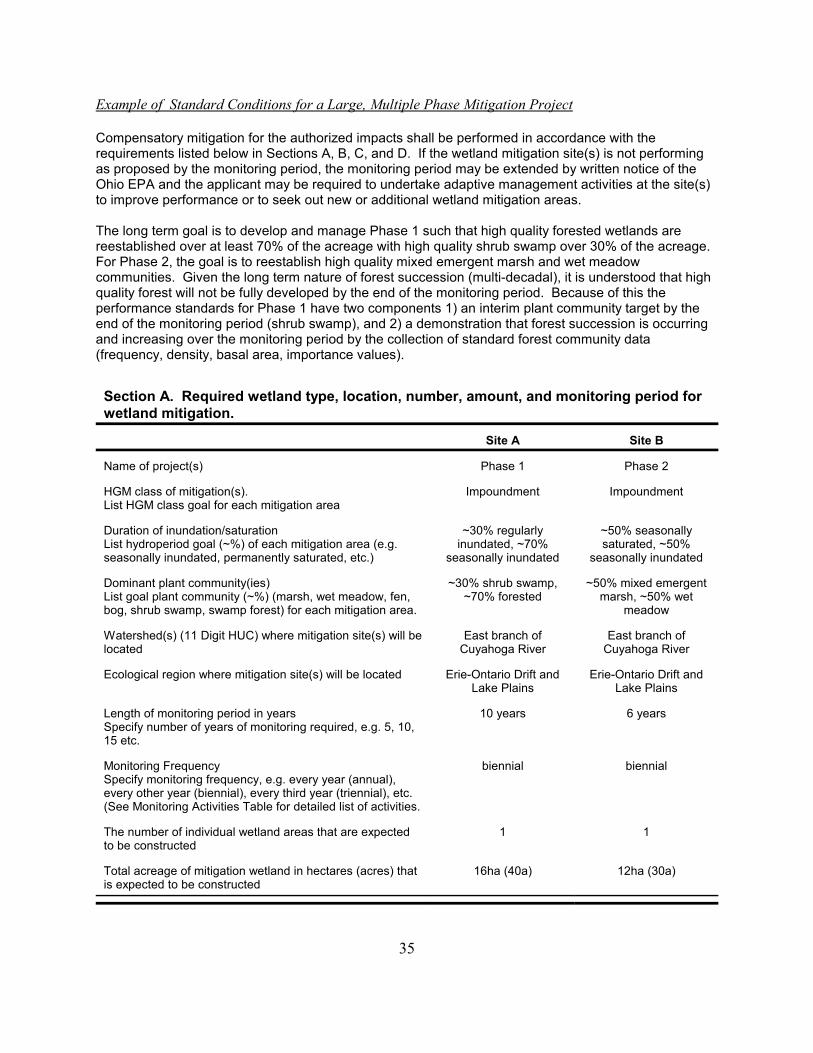
35

Example of Standard Conditions for a Large, Multiple Phase Mitigation Project

Compensatory mitigation for the authorized impacts shall be performed in accordance with therequirements listed below in Sections A, B, C, and D. If the wetland mitigation site(s) is not performingas proposed by the monitoring period, the monitoring period may be extended by written notice of theOhio EPA and the applicant may be required to undertake adaptive management activities at the site(s)to improve performance or to seek out new or additional wetland mitigation areas.

The long term goal is to develop and manage Phase 1 such that high quality forested wetlands arereestablished over at least 70% of the acreage with high quality shrub swamp over 30% of the acreage. For Phase 2, the goal is to reestablish high quality mixed emergent marsh and wet meadowcommunities. Given the long term nature of forest succession (multi-decadal), it is understood that highquality forest will not be fully developed by the end of the monitoring period. Because of this theperformance standards for Phase 1 have two components 1) an interim plant community target by theend of the monitoring period (shrub swamp), and 2) a demonstration that forest succession is occurringand increasing over the monitoring period by the collection of standard forest community data(frequency, density, basal area, importance values).

Section A. Required wetland type, location, number, amount, and monitoring period forwetland mitigation.

Site A Site B

Name of project(s) Phase 1 Phase 2

HGM class of mitigation(s). List HGM class goal for each mitigation area

Impoundment Impoundment

Duration of inundation/saturationList hydroperiod goal (~%) of each mitigation area (e.g.seasonally inundated, permanently saturated, etc.)

~30% regularlyinundated, ~70%

seasonally inundated

~50% seasonallysaturated, ~50%

seasonally inundated

Dominant plant community(ies)List goal plant community (~%) (marsh, wet meadow, fen,bog, shrub swamp, swamp forest) for each mitigation area.

~30% shrub swamp,~70% forested

~50% mixed emergentmarsh, ~50% wet

meadow

Watershed(s) (11 Digit HUC) where mitigation site(s) will belocated

East branch ofCuyahoga River

East branch ofCuyahoga River

Ecological region where mitigation site(s) will be located Erie-Ontario Drift andLake Plains

Erie-Ontario Drift andLake Plains

Length of monitoring period in yearsSpecify number of years of monitoring required, e.g. 5, 10,15 etc.

10 years 6 years

Monitoring FrequencySpecify monitoring frequency, e.g. every year (annual),every other year (biennial), every third year (triennial), etc. (See Monitoring Activities Table for detailed list of activities.

biennial biennial

The number of individual wetland areas that are expectedto be constructed

1 1

Total acreage of mitigation wetland in hectares (acres) thatis expected to be constructed

16ha (40a) 12ha (30a)

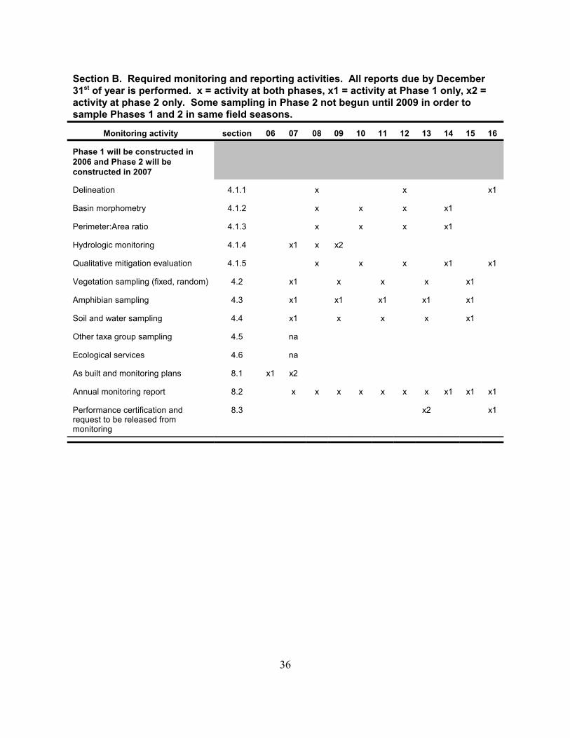
36

Section B. Required monitoring and reporting activities. All reports due by December31st of year is performed. x = activity at both phases, x1 = activity at Phase 1 only, x2 =activity at phase 2 only. Some sampling in Phase 2 not begun until 2009 in order tosample Phases 1 and 2 in same field seasons.

Monitoring activity section 06 07 08 09 10 11 12 13 14 15 16

Phase 1 will be constructed in2006 and Phase 2 will beconstructed in 2007

Delineation 4.1.1 x x x1

Basin morphometry 4.1.2 x x x x1

Perimeter:Area ratio 4.1.3 x x x x1

Hydrologic monitoring 4.1.4 x1 x x2

Qualitative mitigation evaluation 4.1.5 x x x x1 x1

Vegetation sampling (fixed, random) 4.2 x1 x x x x1

Amphibian sampling 4.3 x1 x1 x1 x1 x1

Soil and water sampling 4.4 x1 x x x x1

Other taxa group sampling 4.5 na

Ecological services 4.6 na

As built and monitoring plans 8.1 x1 x2

Annual monitoring report 8.2 x x x x x x x x1 x1 x1

Performance certification andrequest to be released frommonitoring

8.3 x2 x1

37

Section C. Applicable PERFORMANCE STANDARDS.

performance standard

performancestandardsections

check all thatapply to

mitigation siteinsert requested information and/or specify analternative approved performance standard

Acreage 2.1.1 X A total of 28ha (70a) is proposed to be created in twophases, Phase 1 = 16ha (40a), Phase 2 = 12ha (30a)

Basin morphometry 2.1.2 X

Perimeter:Area ratio 2.1.3 X

Hydrologic regime 2.1.4 X

Unvegetated open water 2.2.1 X modified Up to 15% of the wetland area of Phase 2 may beunvegetated open water

Native perennial hydrophytes 2.2.2 X

Invasive species 2.2.3 X

Vegetation - Ecologicstandards

2.2.4 X Phase 1 VIBI-SH (intermediate goal for proposed forestareas; VIBI-F will also be calculated and reported)Minimum VIBI-SH score = 53

Phase 2 VIBI-EMinimum VIBI-E score = 53 (marsh), 60 (wet meadow)

Woody spp. establishment(Shrub Swamps)

2.2.5.1 X

Woody spp. establishment(Swamp Forests)

2.2.5.2 X

Amphibians - Ecologicstandards

2.3 X Phase 1 onlyMinimum AmphIBI score = 20

Other taxa groups - Ecologicstandards

2.4 not applicable

Biogeochemical standards 2.5 X

Ecological services 2.6 not applicable

38

Section D. Applicable monitoring and data analysis requirements.

performance standard

standardmonitoring and data

analysis protocolsections

check all thatapply to

mitigation siteDescribe alternative monitoring and/or dataanalysis requirements

Acreage 4.1.1, 6.1.1 X

Basin morphometry 4.1.2, 6.1.2 X

Perimeter:Area ratio 4.1.3, 6.1.3 X

Hydrologic regime 4.1.4, 6.1.4 X alternative 50 shallow, manually read (weekly) piezometerswill be installed instead of automated levelrecorders and staff gauges

Unvegetated open water 4.2.1, 6.2.1 X

Native perennial hydrophytes 4.2.2, 6.2.2 X

Invasive species 4.2.3, 6.2.3 X

Vegetation sampling - fixedplots only

4.2.6.1, 6.2.4, 6.2.5, 6.2.6

X

Vegetation sampling - fixedand random plots

4.2.6.2, 6.2.4, 6.2.5, 6.2.6

X

Amphibians sampling 4.3, 6.3 X

Other taxa groups - Ecologicstandards

4.4, 6.4 not applicable

Biogeochemical standards 4.5, 6.5 X

Ecological services 4.6, 6.6 not applicable

39

10.0 LITERATURE CITED

Andreas, B.K. and J.J. Mack, and J.S. McCormac.2004. Floristic Quality Assessment Index forVascular Plants and Mosses for the State of Ohio.Wetland Ecology Group, Division of SurfaceWater, Ohio Environmental Protection Agency,Columbus, Ohio. 217 p.

Bedford, B. L. 1999. Cumulative effects onwetland landscapes: links to wetland restorationin the United States and Southern Canada.Wetlands 19:(4):775-788.

Bedford, B. L. 1996. The need to definehydrologic equivalence at the landscape scale forfreshwater wetland mitigation. EcologicalApplications 6(1):57-68.

Brinson, Mark M. 1993. A hydrogeomorphicclassification for wetlands. U.S. Army Corps ofEngineers Waterways Experiment Station.Wetlands Research Program Technical ReportWRP-DE-4. Vicksburg, MS.

Brown, S.C. and J.J. Dinsmore. 1986.Implications of marsh size and isolation for marshbird management. Journal of WildlifeManagement 50:392-397.

D’Avanzo, C. 1990. Long-term evaluation ofwetland creation projects. In Wetland Creationand Restoration: the State of the Science, J.A.Kusler and M.E. Kentula (eds.), p. 487-496.Island Press, Washington, D.C.

Dzubin, A. 1969. Assessing breedingpopulations of ducks by ground counts. Can.Wildl. Serv. Rep. Ser. 6:178-230.

Confer, S.R. and W.A. Niering. 1992.Comparison of created and natural freshwateremergent wetlands in Connecticut (USA).Wetland Ecology and Management 2:142-156.

Fennessy, S., M. Gernes M., J. Mack, DH.Wardrop. 2001. Methods for evaluating wetland

condition: using vegetation to assessenvironmental conditions in wetlands. EPA-822-R-02-020. U.S. Environmental ProtectionAgency; Office of Water; Washington, DC.

Fennessy, M.S., J.J. Mack, A. Rokosch, M.Micacchion, and M. Knapp. 2004. IntegratedWetland Assessment Program. Part 5:Biogeochemical and Hydrological Investigationsof Natural and Mitigation Wetlands. Ohio EPATechnical Report WET/2004-5. OhioEnvironmental Protection Agency, WetlandEcology Group, Division of Surface Water,Columbus, Ohio.

Fennessy, M.S and J. Roehrs. 1997. A functionalassessment of mitigation wetlands in Ohio:comparisons with natural systems. Final report tothe U.S. Environmental Protection Agency, June1997, Ohio Environmental Protection Agency,Division of Surface Water, Wetlands Unit,Columbus, Ohio.

Gibbs, J.P. and S.M. Melvin. 1997. Power todetect trends in waterbird abundance with call-response surveys. Journal of WildlifeManagement 61:1262-1267.

Gauch, H.G. 1982. Multivariate analysis incommunity ecology. Cambridge University Press,New York. 298p.

Griffiths, R.A. and T.J.C. Beebee. 1992. Declineand Fall of Amphibians. New Scientist 27:25-29.

Inman, R.L. H.H. Prince and D.B. Hayes. 2002.Avian communities in forested riparian wetlandsof southern Michigan, USA. Wetlands(22)(4):647-660.

Kentula, M.E., R.P. Brooks, S.E. Gwin, C.C.Holland, A.D. Sherman, J.C. Sifneos. 1992.Wetlands - an approach to improving decisionmaking in wetland restoration and creation.Island Press, Washington DC.

40

Knapp, M. 2004. Integrated wetland assessmentprogram. Part 8: wetland invertebrate communityindex (WICI). Ohio EPA Technical ReportWET/2004-8. Ohio Environmental ProtectionAgency, Division of Surface Water, EcologicalAssessment Section, Columbus, Ohio.

Mack, J.J. 2001. Ohio Rapid Assessment Methodfor Wetlands, Manual for Using Version 5.0.Ohio EPA Technical Bulletin WET2001-1. OhioEnvironmental Protection Agency, Division ofSurface Water, 401 Wetland Ecology Unit,Columbus, Ohio.

Mack, J.J. 2004a. Integrated wetland assessmentprogram. Part 2: an ordination and classificationof wetlands in the Till and Lake Plains andAllegheny Plateau regions. Ohio EPA TechnicalReport WET/2004-2. Ohio EnvironmentalProtection Agency, Division of Surface Water,Wetland Ecology Group, Columbus, Ohio.

Mack, J.J. 2004b. Integrated wetland assessmentprogram. Part 4: vegetation index of bioticintegrity (VIBI) for Ohio wetlands. Ohio EPATechnical Report WET/2004-4. OhioEnvironmental Protection Agency, Division ofSurface Water, Wetland Ecology Group,Columbus, Ohio.

Mack, J.J. 2004c. Integrated wetland assessmentprogram. Part 9: field manual for the vegetationindex of biotic integrity for wetlands v. 1.3. OhioEPA Technical Report WET/2004-9. OhioEnvironmental Protection Agency, Division ofSurface Water, Wetland Ecology Group,Columbus, Ohio.

McCune B. and J. Mefford. 1999. MultivariateAnalysis of Ecological Data. V. 4.0. MjMSoftware. Glenenden Beach, Oregon. USA.

Micacchion, M. 2004. Integrated wetlandassessment program. Part 7: amphibian index ofbiotic integrity for Ohio wetlands. Ohio EPATechnical Report WET/2004-7. OhioEnvironmental Protection Agency, Division of

Surface Water, Wetland Ecology Group,Columbus, Ohio.

Mitsch, W. J. and J.G. Gosselink. 2000.Wetlands, 3rd Ed. John Wiley and Sons, Inc.,New York, NY.

Mitsch, W.J., X. Wu, R.W. Nairn, P.E. Weihe, N.Wang, R. Deal, and C.E. Boucher. 1998. Creatingand restoring wetlands: A whole-ecosystemexperiment in self-design. Bioscience 48:1019-1030.

Mitsch, W.J. and R.F. Wilson. 1996. Improvingthe success of wetland creation and restorationwith know-how, time, and self-design. EcologicalApplications 6:77-83.

Mueller-Dombois, Dieter and Hans Ellenberg.1974. Aims and Methods of Vegetation Ecology.John Wiley & Sons Press.

National Research Council. 2001. Compensatingfor Wetland Losses Under the Clean Water Act.National Academy Press, Washington, D.C.

NCR. 1998. Recommended soil test proceduresfor the North Central Region. North CentralRegional Research Publication No. 221 (revised).Missouri Agricultural Experiment Station SB1001. Revised January 1998.

Ohio EPA. 1988. Biological criteria for theprotection of aquatic life: Volume 1: the role ofbiological data in water quality assessment. OhioEnvironmental Protection Agency, EcologicalAssessment Section, Columbus, Ohio.

Ohio EPA. 1989. Biological criteria for theprotection of aquatic life: Volume III:Standardized biological field sampling andlaboratory methods for assessing fish andmacroinvertebrate communities. OhioEnvironmental Protection Agency, EcologicalAssessment Section, Columbus, Ohio.

41

Peet, R.K., T.R. Wentworth, and P.S. White.1988. A flexible, multipurpose method forrecording vegetation composition and structure.Castanea 63(3): 262-274.

Petranka, J.W., S.S. Murray, and C.A. Kennedy.2003. Responses of amphibians to restoration ofa southern Appalachian wetland: perturbationsconfound post-restoration assessment. Wetlands23:278-290.

Porej, D. 2003. An inventory of Ohio wetlandcompensatory mitigation. Final Report to U.S.EPA Grant No. CD975762. Ohio EnvironmentalProtection Agency, Division of Surface Water,Wetland Ecology Group, Columbus, Ohio.

Porej, D. 2004. Faunal aspects of wetlandcreation and restoration. PhD. Dissertation. TheOhio State University, Columbus, OH.

Porej, D., M. Micacchion and T.E. Hetherington.2004. Core Terrestrial Habitat for Conservation ofLocal Populations of Salamanders and WoodFrogs in Agricultural Landscapes. BiologicalConservation120:399-410.

Ralph, C.J., J.R. Sauer and S. Droege. 1995.Monitoring bird populations by point counts.PSW-GTR-149. U.S. Forest Service, PacificResearch Station, Albany, CA.

Ribie C.A., S.J. Lewis, S. Melvin, J. Bart, B.Peterjohn. 1999. Proceedings of the marsh birdmonitoring workshop. U.S. Fish and WildlifeService, Patuxent Research Refuge, Laurel, MD.

Schmida, A., 1984. Whittaker’s plant diversitysampling method. Israel Journal of Botany, 33,41-46.

Smith, R.D., A. Ammann, C. Bartoldus, and M.M.Brinson. 1995. An approach for assessingwetland functions using hydrogeomorphicclassification, reference wetlands, and functionalindices. Technical Report WRP-DE-9.

Waterways Experiment Station, U.S. Army Corpsof Engineers, Vicksburg, Mississippi.

ter Braak, C.F. 1987. The analysis of vegetation-environment relationships with canonicalcorrespondence analysis. Vegetation 64:69-77.

U.S. Army Corps of Engineers. 1987. FederalManual for the Delineation of Wetlands.

U.S. Environmental Protection Agency. 1997.Level III ecoregions of the continental UnitedStates (revision of Omernik, 1987). Corvallis,Oregon, U.S. EPA - National Health andEnvironmental Research Laboratory Map —1,various scales.

Wake, D. B. 1991. Declining AmphibianPopulations. Science 253:860.

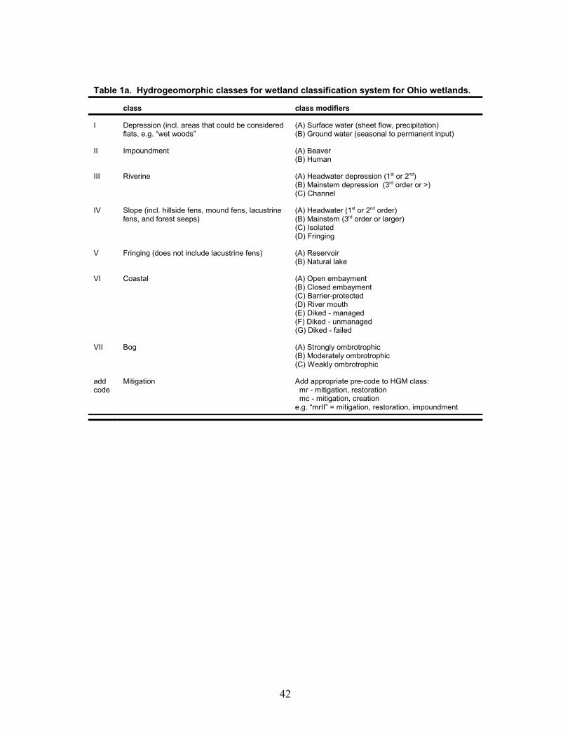
42

Table 1a. Hydrogeomorphic classes for wetland classification system for Ohio wetlands.

class class modifiers

I Depression (incl. areas that could be consideredflats, e.g. “wet woods”

(A) Surface water (sheet flow, precipitation)(B) Ground water (seasonal to permanent input)

II Impoundment (A) Beaver(B) Human

III Riverine (A) Headwater depression (1st or 2nd)(B) Mainstem depression (3rd order or >)(C) Channel

IV Slope (incl. hillside fens, mound fens, lacustrinefens, and forest seeps)

(A) Headwater (1st or 2nd order)(B) Mainstem (3rd order or larger)(C) Isolated(D) Fringing

V Fringing (does not include lacustrine fens) (A) Reservoir(B) Natural lake

VI Coastal (A) Open embayment(B) Closed embayment(C) Barrier-protected(D) River mouth(E) Diked - managed(F) Diked - unmanaged(G) Diked - failed

VII Bog (A) Strongly ombrotrophic(B) Moderately ombrotrophic(C) Weakly ombrotrophic

addcode

Mitigation Add appropriate pre-code to HGM class: mr - mitigation, restoration mc - mitigation, creatione.g. “mrII” = mitigation, restoration, impoundment

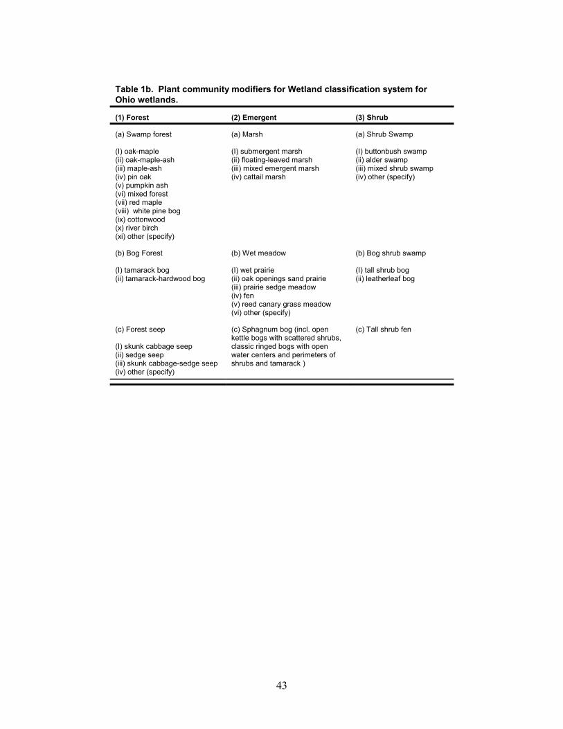
43

Table 1b. Plant community modifiers for Wetland classification system forOhio wetlands.

(1) Forest (2) Emergent (3) Shrub

(a) Swamp forest

(I) oak-maple(ii) oak-maple-ash(iii) maple-ash(iv) pin oak(v) pumpkin ash(vi) mixed forest(vii) red maple(viii) white pine bog(ix) cottonwood(x) river birch(xi) other (specify)

(a) Marsh

(I) submergent marsh(ii) floating-leaved marsh(iii) mixed emergent marsh(iv) cattail marsh

(a) Shrub Swamp

(I) buttonbush swamp(ii) alder swamp(iii) mixed shrub swamp(iv) other (specify)

(b) Bog Forest

(I) tamarack bog(ii) tamarack-hardwood bog

(b) Wet meadow

(I) wet prairie(ii) oak openings sand prairie(iii) prairie sedge meadow(iv) fen(v) reed canary grass meadow(vi) other (specify)

(b) Bog shrub swamp

(I) tall shrub bog(ii) leatherleaf bog

(c) Forest seep

(I) skunk cabbage seep(ii) sedge seep(iii) skunk cabbage-sedge seep(iv) other (specify)

(c) Sphagnum bog (incl. openkettle bogs with scattered shrubs,classic ringed bogs with openwater centers and perimeters ofshrubs and tamarack )

(c) Tall shrub fen

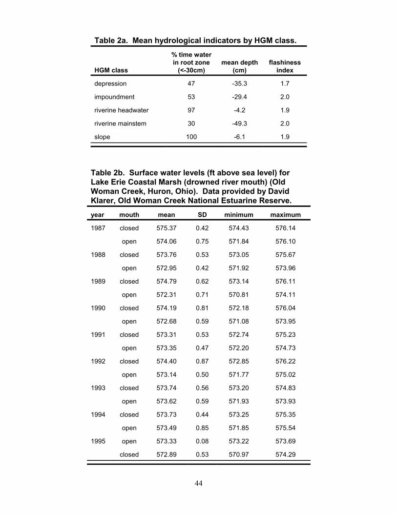
44

Table 2a. Mean hydrological indicators by HGM class.

HGM class

% time waterin root zone

(<-30cm)mean depth

(cm)flashiness

index

depression 47 -35.3 1.7

impoundment 53 -29.4 2.0

riverine headwater 97 -4.2 1.9

riverine mainstem 30 -49.3 2.0

slope 100 -6.1 1.9

Table 2b. Surface water levels (ft above sea level) forLake Erie Coastal Marsh (drowned river mouth) (OldWoman Creek, Huron, Ohio). Data provided by DavidKlarer, Old Woman Creek National Estuarine Reserve. year mouth mean SD minimum maximum

1987 closed 575.37 0.42 574.43 576.14

open 574.06 0.75 571.84 576.10

1988 closed 573.76 0.53 573.05 575.67

open 572.95 0.42 571.92 573.96

1989 closed 574.79 0.62 573.14 576.11

open 572.31 0.71 570.81 574.11

1990 closed 574.19 0.81 572.18 576.04

open 572.68 0.59 571.08 573.95

1991 closed 573.31 0.53 572.74 575.23

open 573.35 0.47 572.20 574.73

1992 closed 574.40 0.87 572.85 576.22

open 573.14 0.50 571.77 575.02

1993 closed 573.74 0.56 573.20 574.83

open 573.62 0.59 571.93 573.93

1994 closed 573.73 0.44 573.25 575.35

open 573.49 0.85 571.85 575.54

1995 open 573.33 0.08 573.22 573.69

closed 572.89 0.53 570.97 574.29

45

Table 3a. Ranges for Vegetation IBI scores for Category 2 and 3 Wetlands by hydrogeomorphic(HGM) class, HGM subclass, plant community class, and ecoregion. Ranges are from Table 7INTEGRATED WETLAND ASSESSMENT PROGRAM. Part 9: Field Manual for the Vegetation Index ofBiotic Integrity for Wetlands v. 1.3, Ohio EPA Technical Report WET/2004-9. HGM classes and plantcommunity classes defined in Tables 8A and 8B of INTEGRATED WETLAND ASSESSMENTPROGRAM. Part 9: Field Manual for the Vegetation Index of Biotic Integrity for Wetlands v. 1.3, OhioEPA Technical Report WET/2004-9. EOLP = Erie-Ontario Drift and Lake Plains (glaciated AlleghenyPlateau) (see Figure 1).

HGM class HGM subclass plant community ecoregionsWLH

(Category 2)SWLH

(Category 3)

Depression all Swamp forest, Marsh, Shrubswamp

EOLP

all other regions

61 - 75

51 - 62

76 - 100

63 - 100

all Wet Meadow (incl. prairies andsedge/grass dominatedcommunities that are not slopes)

all regions 60 - 75 76 - 100

Impoundment all Marsh, Shrub Swamp EOLP

all other regions

53 - 66

48 - 63

67 - 100

64 - 100

Wet Meadow (incl. prairies andsedge/grass dominatedcommunities that are not slopes)

all regions 60 - 75 76 - 100

Riverine Headwater all EOLP

all other regions

57 - 69

47 - 59

70 - 100

60 - 100

Mainstem andChannel

all EOLP

all other regions

57 - 73

42 - 52

74 - 100

53 - 100

Headwater orMainstem

Wet Meadow (incl. prairies andsedge/grass dominatedcommunities that are not slopes)

all regions 60 - 75 76 - 100

Slope all (includeslacustrine fens)

Wet meadow (fen), tall shrub fen,forest seep

all regions 60 - 75 76 - 100

Fringing1 Natural Lakes(excludinglacustrine fens)and reservoirs

tbd tbd tbd tbd

Coastal closedembayment,barrier-protected,river mouth

all all regions 50 - 61 62 - 100

open embayment,diked (managedunmanaged failed)

tbd2 tbd tbd tbd

Bog weaklyombrotrophic

Tamarack-hardwood bog, Tallshrub bog

all regions 66 - 82 83 - 100

moderate-stronglyombrotrophic

Tamarack forest, Leatherleaf bog Sphagnum bog

all regions 48 - 59 60 - 100

1. Depending on the circumstances, scoring breaks for depression, impoundment, or riverine should be used.2. Scoring breaks for coastal embayment, barrier-protected, and river mouth should be used.

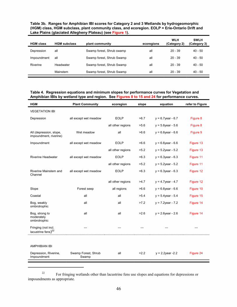
22 For fringing wetlands other than lacustrine fens use slopes and equations for depressions orimpoundments as appropriate.

46

Table 3b. Ranges for Amphibian IBI scores for Category 2 and 3 Wetlands by hydrogeomorphic(HGM) class, HGM subclass, plant community class, and ecoregion. EOLP = Erie-Ontario Drift andLake Plains (glaciated Allegheny Plateau) (see Figure 1).

HGM class HGM subclass plant community ecoregionsWLH

(Category 2)SWLH

(Category 3)

Depression all Swamp forest, Shrub swamp all 20 - 39 40 - 50

Impoundment all Swamp forest, Shrub Swamp all 20 - 39 40 - 50

Riverine Headwater Swamp forest, Shrub Swamp all 20 - 39 40 - 50

Mainstem Swamp forest, Shrub Swamp all 20 - 39 40 - 50

Table 4. Regression equations and minimum slopes for performance curves for Vegetation andAmphibian IBIs by wetland type and region. See Figures 8 to 15 and 24 for performance curves.

HGM Plant Community ecoregion slope equation refer to Figure

VEGETATION IBI

Depression all except wet meadow EOLP >6.7 y = 6.7year - 6.7 Figure 8

all other regions >5.6 y = 5.6year - 5.6 Figure 8

All (depression, slope,impoundment, riverine)

Wet meadow all >6.6 y = 6.6year - 6.6 Figure 9

Impoundment all except wet meadow EOLP >6.6 y = 6.6year - 6.6 Figure 13

all other regions >5.2 y = 5.2year - 5.2 Figure 13

Riverine Headwater all except wet meadow EOLP >6.3 y = 6.3year - 6.3 Figure 11

all other regions >5.2 y = 5.2year - 5.2 Figure 11

Riverine Mainstem andChannel

all except wet meadow EOLP >6.3 y = 6.3year - 6.3 Figure 12

all other regions >4.7 y = 4.7year - 4.7 Figure 12

Slope Forest seep all regions >6.6 y = 6.6year - 6.6 Figure 10

Coastal all all >5.4 y = 5.4year - 5.4 Figure 15

Bog, weaklyombrotrophic

all all >7.2 y = 7.2year - 7.2 Figure 14

Bog, strong tomoderatelyombrotrophic

all all >2.6 y = 2.6year - 2.6 Figure 14

Fringing (not incl.lacustrine fens)22

--- --- --- --- ---

AMPHIBIAN IBI

Depression, Riverine,Impoundment

Swamp Forest, ShrubSwamp

all >2.2 y = 2.2year -2.2 Figure 24

47

Table 5. Performance standards for wetland soils. Standards for total N for non-marsh systems notproposed.

HGM class Plant community % solidstotal Organic

Carbon (TOC) (%) total N (%)

Depression Marshes < 62.4 > 3.6 > 0.5

Shrub swamps < 41.9 > 10.1 ---

Forests (vernal pools) < 58.1 > 5.4 ---

Forests (wet woods) < 57.4 > 6.6 ---

Wet meadows (wet prairie,prairie sedge meadow,other, etc.)

< 55.9 > 3.1 > 0.5

Wet meadows - LakePlains Sand Prairies

< 61.0 > 9.5 ---

Impoundment Marshes < 46.6 > 3.9 > 0.5

Shrub swamps < 62.1 > 3.7 ---

Riverine mainstem Marshes < 46.6 > 3.9 > 0.5

Shrub swamps < 62.1 > 3.7 ---

Swamp forests < 66.1 > 2.9 ---

Riverine headwater Marshes, shrub swamps < 46.6 > 4.1 > 0.5

Slope Fen (calcareous) < 30.0 > 24.5 ---

Fen (other) < 48.0 > 9.0 ---

Forest seeps < 38.0 > 9.3 ---

Coastal all < 54.9 > 4.1 > 0.5

Bog all < 18.9 > 41.7 ---

48

Table 6a. Conceptual 5 year schedule for required monitoring andreporting activities. All reports due by December 31st of year activity isperformed.

Monitoring activity section 0 1 2 3 4 5

Site was (will be) constructed in _________(insert year)

Delineation 4.1.1 x x

Basin morphometry 4.1.2 x x

Perimeter:Area ratio 4.1.3 x x

Hydrologic monitoring 4.1.4 x x

Qualitative mitigation evaluation 4.1.5 x x

Vegetation sampling (fixed, random) 4.2 x x x

Amphibian sampling 4.3 x x x

Soil and water sampling 4.4 x x x

Other taxa group sampling 4.5 x x x

Ecological services 4.6 x x x

As built plans and monitoring plan 8.1 x

Annual monitoring report 8.2 x x x x x

Performance certification and request to bereleased from monitoring

8.3 x

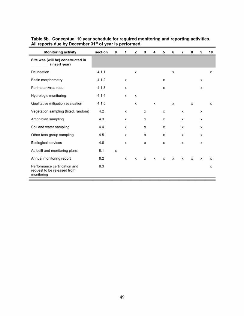
49

Table 6b. Conceptual 10 year schedule for required monitoring and reporting activities. All reports due by December 31st of year is performed.

Monitoring activity section 0 1 2 3 4 5 6 7 8 9 10

Site was (will be) constructed in_________ (insert year)

Delineation 4.1.1 x x x

Basin morphometry 4.1.2 x x x

Perimeter:Area ratio 4.1.3 x x x

Hydrologic monitoring 4.1.4 x x

Qualitative mitigation evaluation 4.1.5 x x x x x

Vegetation sampling (fixed, random) 4.2 x x x x x

Amphibian sampling 4.3 x x x x x

Soil and water sampling 4.4 x x x x x

Other taxa group sampling 4.5 x x x x x

Ecological services 4.6 x x x x x

As built and monitoring plans 8.1 x

Annual monitoring report 8.2 x x x x x x x x x x

Performance certification andrequest to be released frommonitoring

8.3 x

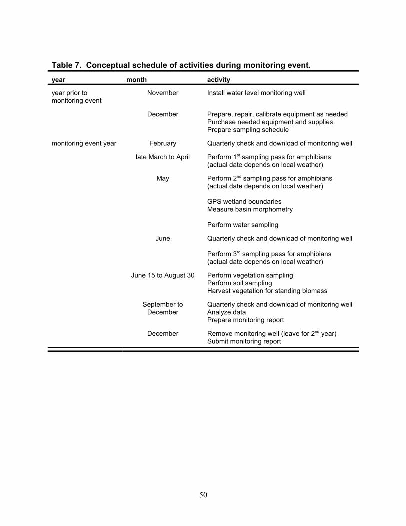
50

Table 7. Conceptual schedule of activities during monitoring event.year month activity

year prior tomonitoring event

November Install water level monitoring well

December Prepare, repair, calibrate equipment as neededPurchase needed equipment and suppliesPrepare sampling schedule

monitoring event year February Quarterly check and download of monitoring well

late March to April Perform 1st sampling pass for amphibians(actual date depends on local weather)

May Perform 2nd sampling pass for amphibians(actual date depends on local weather)

GPS wetland boundariesMeasure basin morphometry

Perform water sampling

June Quarterly check and download of monitoring well

Perform 3rd sampling pass for amphibians (actual date depends on local weather)

June 15 to August 30 Perform vegetation samplingPerform soil samplingHarvest vegetation for standing biomass

September toDecember

Quarterly check and download of monitoring wellAnalyze dataPrepare monitoring report

December Remove monitoring well (leave for 2nd year)Submit monitoring report

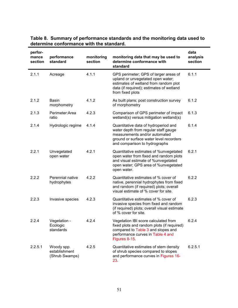
51

Table 8. Summary of performance standards and the monitoring data used todetermine conformance with the standard.perfor-mancesection

performancestandard

monitoringsection

monitoring data that may be used todetermine conformance withstandard

dataanalysissection

2.1.1 Acreage 4.1.1 GPS perimeter; GPS of larger areas ofupland or unvegetated open water;estimates of wetland from random plotdata (if required); estimates of wetlandfrom fixed plots

6.1.1

2.1.2 Basinmorphometry

4.1.2 As built plans; post construction surveyof morphometry

6.1.2

2.1.3 Perimeter:Arearatio

4.2.3 Comparison of GPS perimeter of impactwetland(s) versus mitigation wetland(s)

6.1.3

2.1.4 Hydrologic regime 4.1.4 Quantitative data of hydroperiod andwater depth from regular staff gaugemeasurements and/or automatedground or surface water level recordersand comparison to hydrographs

6.1.4

2.2.1 Unvegetatedopen water

4.2.1 Quantitative estimates of %unvegetatedopen water from fixed and random plotsand visual estimate of %unvegetatedopen water; GPS area of %unvegetatedopen water.

6.2.1

2.2.2 Perennial nativehydrophytes

4.2.2 Quantitative estimates of % cover ofnative, perennial hydrophytes from fixedand random (if required) plots; overallvisual estimate of % cover for site.

6.2.2

2.2.3 Invasive species 4.2.3 Quantitative estimates of % cover ofinvasive species from fixed and random(if required) plots; overall visual estimateof % cover for site.

6.2.3

2.2.4 Vegetation -Ecologicstandards

4.2.4 Vegetation IBI score calculated fromfixed plots and random plots (if required)compared to Table 3 and slopes andperformance curves in Table 4 andFigures 8-15.

6.2.4

2.2.5.1 Woody spp.establishment(Shrub Swamps)

4.2.5 Quantitative estimates of stem densityof shrub species compared to slopesand performance curves in Figures 16-23.

6.2.5.1

Table 8. Summary of performance standards and the monitoring data used todetermine conformance with the standard.perfor-mancesection

performancestandard

monitoringsection

monitoring data that may be used todetermine conformance withstandard

dataanalysissection

52

2.2.5.2 Woody spp.establishment(Swamp Forests)

4.2.5 Quantitative estimates of stem densityof shrub species, subcanopy treespecies, 0-5cm tree species, 5-15cmtree species compared to slopes andperformance curves in Figures 16-23.

6.2.5.2

2.3 Amphibians -Ecologicstandards

4.3 Amphibian IBI score calculatedcompared to slopes and performancecurves in Table 3 and Figure 24.

6.3

2.4 Other taxa groups- Ecologicstandards

4.4 Quantitative measurements comparedto numeric goals for taxa group usingappropriate sampling methodology

6.4

2.5 Biogeochemicalstandards

4.5 Quantitative measurements of TotalOrganic Carbon (%), total solids (%),and total Nitrogen (%). Comparison tomedian values and 25th and 75th

percentiles of appropriate RestorationTemplate in Table 5.

6.5

2.6 Ecologicalservices

4.6 Quantitative measurements comparedto numeric goals for specific (ecologicalservice (function or value) usingappropriate sampling methodology

6.6

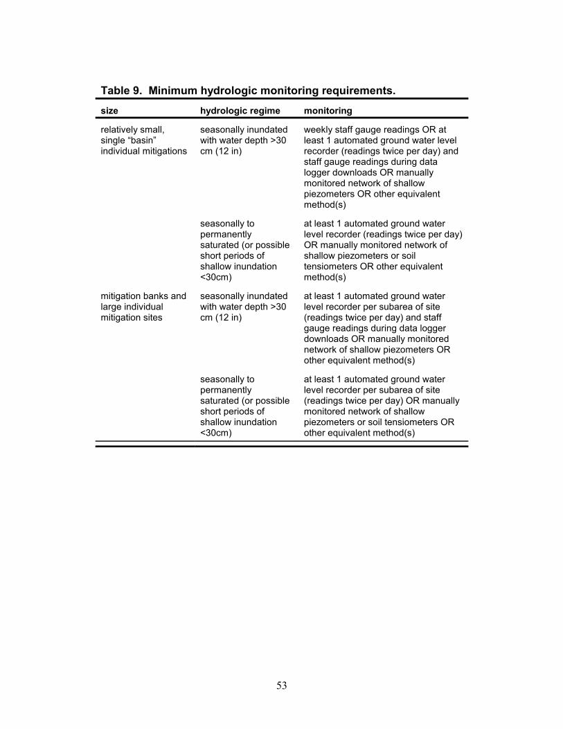
53

Table 9. Minimum hydrologic monitoring requirements.size hydrologic regime monitoring

relatively small,single “basin”individual mitigations

seasonally inundatedwith water depth >30cm (12 in)

weekly staff gauge readings OR atleast 1 automated ground water levelrecorder (readings twice per day) andstaff gauge readings during datalogger downloads OR manuallymonitored network of shallowpiezometers OR other equivalentmethod(s)

seasonally topermanentlysaturated (or possibleshort periods ofshallow inundation<30cm)

at least 1 automated ground waterlevel recorder (readings twice per day)OR manually monitored network ofshallow piezometers or soiltensiometers OR other equivalentmethod(s)

mitigation banks andlarge individualmitigation sites

seasonally inundatedwith water depth >30cm (12 in)

at least 1 automated ground waterlevel recorder per subarea of site(readings twice per day) and staffgauge readings during data loggerdownloads OR manually monitorednetwork of shallow piezometers ORother equivalent method(s)

seasonally topermanentlysaturated (or possibleshort periods ofshallow inundation<30cm)

at least 1 automated ground waterlevel recorder per subarea of site(readings twice per day) OR manuallymonitored network of shallowpiezometers or soil tensiometers ORother equivalent method(s)

54

Tabl

e 1

0. S

umm

ary

of v

eget

atio

n su

rvey

dat

a ty

pes,

des

crip

tions

, and

qua

lity

assu

ranc

e pr

oced

ures

for p

lot b

ased

veg

etat

ion

sam

plin

gm

etho

d sp

ecifi

ed.

data

type

desc

riptio

nda

ta q

ualit

y pr

oced

ures

pres

ence

Pres

ence

/abs

ence

. D

eter

min

ing

that

a p

artic

ular

pla

ntsp

ecie

s is

pre

sent

in th

e su

rvey

plo

t1.

use

of n

este

d qu

adra

ts w

hich

requ

ire c

lose

exa

min

atio

n of

sm

all a

rea

follo

wed

by

exam

inat

ion

of la

rger

and

larg

er q

uadr

ats

2. c

olle

ctio

n of

vou

cher

spe

cim

ens

of d

iffic

ult g

ener

a or

fam

ilies

or p

lant

s un

able

to b

e id

entif

ied

in th

e fie

ld fo

r lat

er id

entif

icat

ion

in th

e la

b3.

pro

perly

and

com

plet

ely

fillin

g ou

t the

dat

a fo

rm a

nd re

view

ing

the

data

form

fo

r com

plet

enes

s im

med

iate

ly a

fter t

he s

urve

y is

com

plet

ed4.

col

lect

ion

of d

ata

by tr

aine

d fie

ld b

otan

ists

% c

over

estim

ate

of p

erce

nt c

over

of p

lant

spe

cies

, litt

er c

o ve

r,an

d op

en w

ater

cov

er d

eter

min

ed to

be

pres

ent i

n th

esu

rvey

plo

t

1. u

se o

f "do

ublin

g" c

over

cla

sses

whi

ch e

nabl

e re

prod

ucib

le c

ove

clas

sas

sign

men

ts b

y di

ffere

nt u

sers

2. p

rope

rly a

nd c

ompl

etel

y fil

ling

out t

he d

ata

form

and

revi

ewin

g th

e da

ta fo

rm

for c

ompl

eten

ess

imm

edia

tely

afte

r the

sur

vey

is c

ompl

eted

3. c

olle

ctio

n of

dat

a by

trai

ned

field

bot

anis

ts

diam

eter

at b

reas

t hei

ght (

dbh)

mea

surin

g th

e db

h of

a tr

ee o

r shr

ub a

t "br

east

hei

ght"

usin

g a

dbh

tape

mea

sure

.1.

usi

ng p

rofe

ssio

nal d

bh ta

pe a

nd ta

king

mea

sure

men

ts a

t sam

e he

ight

2. t

rain

ing

user

s on

pro

per m

etho

d fo

r usi

ng a

nd re

adin

g ta

pe3.

pro

perly

and

com

plet

ely

fillin

g ou

t the

dat

a fo

rm a

nd re

view

ing

the

data

form

fo

r com

plet

enes

s im

med

iate

ly a

fter t

he s

urve

y is

com

plet

ed

stem

cou

nts

coun

ting

ever

y w

oody

pla

nt a

bove

1m

hig

h in

the

entir

esu

rvey

plo

t1.

tra

inin

g us

ers

on s

ampl

ing

met

hod

proc

edur

es.

2. p

rope

rly a

nd c

ompl

etel

y fil

ling

out t

he d

ata

form

and

revi

ewin

g th

e da

ta fo

rm

for c

ompl

eten

ess

imm

edia

tely

afte

r the

sur

vey

is c

ompl

eted

wat

er d

epth

mea

surin

g th

e de

pth

of w

ater

in th

e ce

nter

s of

the

inte

nsiv

e m

odul

es in

the

surv

ey p

lot u

sing

a m

eter

stic

kse

e ab

ove

litte

r dep

thm

easu

ring

the

dept

h of

litte

r in

the

cent

ers

of th

ein

tens

ive

mod

ules

in th

e su

rvey

plo

t by

digg

ing

a sm

all

test

hol

e an

d m

easu

ring

the

dept

h w

ith a

rule

r

see

abov

e

dept

h to

sat

urat

ed s

oil

mea

surin

g th

e de

pth

until

sat

urat

ed s

oils

are

reac

hed

inth

e ce

nter

s of

the

inte

nsiv

e m

odul

es in

the

surv

ey p

lot b

ydi

ggin

g a

smal

l tes

t hol

e an

d m

easu

ring

the

dept

h w

ith a

rule

r

see

abov

e

woo

dy d

ebris

cou

nts

coun

ting

ever

y pi

ece

of c

ours

e w

oody

deb

ris in

the

inte

nsiv

e m

odul

es g

reat

er th

an 1

0cm

in

diam

eter

see

abov

e

stan

ding

bio

mas

sha

rves

ting

to g

roun

d le

vel a

ll pl

ant m

ater

ial r

oote

d in

a0.

1m2 q

uadr

at o

f the

8 (t

ypic

al) n

este

d qu

adra

ts, d

ryin

gth

e m

ater

ial a

nd w

eigh

ing

it.

1 an

d 2

abov

e an

d us

e pr

oper

ly c

alib

rate

d sc

ale

tuss

ock/

hum

moc

k co

unts

coun

ting

the

num

ber o

f tus

sock

s an

d hu

mm

ocks

in th

ein

tens

ive

mod

ules

se

e ab

ove

mic

roha

bita

t int

ersp

ersi

ones

timat

ing

the

over

all a

mou

nt o

f mic

roha

bita

t usi

ng a

qual

itativ

e m

icro

habi

tat i

nter

sper

sion

sca

lese

e ab

ove

55

Table 11. Analytical parameters and suggested methodsfor soil analysis.parameter method

pH SW846-9045C (soil)

P, Bray 1 (weak) NRC-13

P, Bray 2 (strong) NRC-13 (acid concentration 4X weak Bray)

Cation Exchange Capacity NRC-13

Exchangeable Ca, Mg, K NRC -13

Total Organic Carbon USEPA 415.1, LECO2000 Analyzer, CEInstruments CHN-Analyzer (Model nc-2100),or equivalent method

Total Nitrogen USEPA 415.1, LECO2000 Analyzer, CEInstruments CHN-Analyzer (Model nc-2100),or equivalent method

Total solids USEPA 160.3

56

Table 12. Example of summary table for VIBI scores, metricvalues, and chemistry data.

parameter year 1 year 3 year 5 year 7 year 9

VIBI - E score

Metric 1 Carex richness

Metric 2 Dicot richness

Metric 3 Shrub richness

Metric 4 Hydrophyte Richness

etc. cont. with other metrics

Total organic carbon

%Nitrogen

etc. cont. with other chemistry

Coarse woody debris

Depth to saturated soil

etc. continue other parameters

57

Table 13. Example of summary table for VIBI scores, metric values, andchemistry data for multiple sites.

parameter parameter year 1 year 3 year 5 year 7 year 9

Site A (or Plot 1) VIBI - E score

Metric 1 Carex richness

Metric 2 Dicot richness etc.

Total organic carbon

%Nitrogen etc.

Site B (or Plot 2) VIBI - E score

Metric 1 Carex richness

Metric 2 Dicot richness etc.

Total organic carbon

%Nitrogen etc.

Site C (or Plot 3) VIBI - E score

Metric 1 Carex richness

Metric 2 Dicot richness etc.

Total organic carbon

%Nitrogen etc.

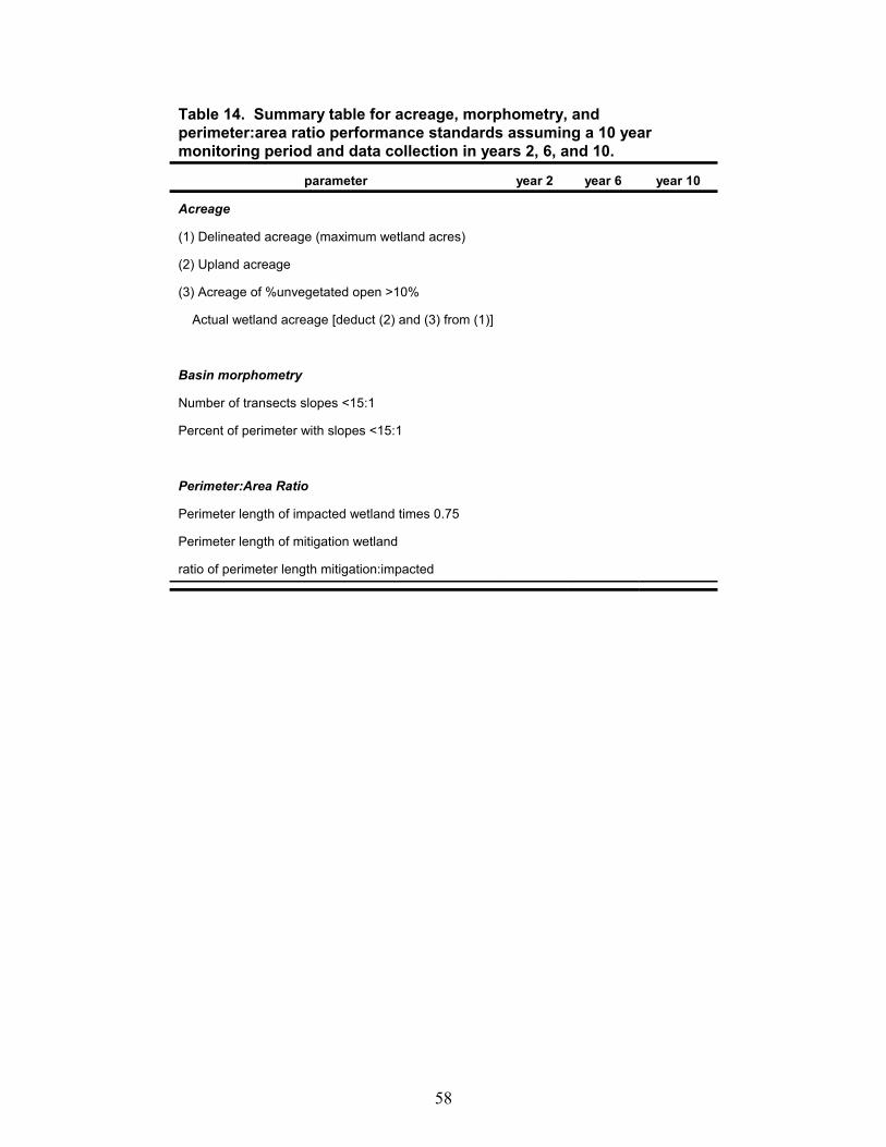
58

Table 14. Summary table for acreage, morphometry, andperimeter:area ratio performance standards assuming a 10 yearmonitoring period and data collection in years 2, 6, and 10.

parameter year 2 year 6 year 10

Acreage

(1) Delineated acreage (maximum wetland acres)

(2) Upland acreage

(3) Acreage of %unvegetated open >10%

Actual wetland acreage [deduct (2) and (3) from (1)]

Basin morphometry

Number of transects slopes <15:1

Percent of perimeter with slopes <15:1

Perimeter:Area Ratio

Perimeter length of impacted wetland times 0.75

Perimeter length of mitigation wetland

ratio of perimeter length mitigation:impacted

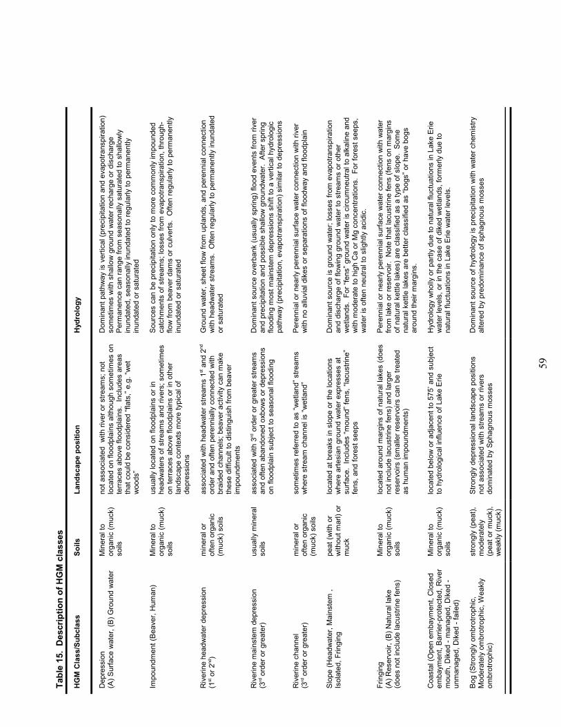
59

Tabl

e 15

. D

escr

iptio

n of

HG

M c

lass

es

HG

M C

lass

/Sub

clas

sSo

ilsLa

ndsc

ape

posi

tion

Hyd

rolo

gy

Dep

ress

ion

(A) S

urfa

ce w

ater

, (B)

Gro

und

wat

erM

iner

al to

orga

nic

(muc

k)so

ils

not a

ssoc

iate

d w

ith ri

ver o

r stre

ams;

not

loca

ted

on fl

oodp

lain

s al

thou

gh s

omet

imes

on

terra

ces

abov

e flo

odpl

ains

. In

clud

es a

reas

that

cou

ld b

e co

nsid

ered

“fla

ts,”

e.g.

“wet

woo

ds”

Dom

inan

t pat

hway

is v

ertic

al (p

reci

pita

tion

and

evap

otra

nspi

ratio

n)so

met

imes

with

sha

llow

gro

und

wat

er re

char

ge o

r dis

char

gePe

rman

ence

can

rang

e fro

m s

easo

nally

sat

urat

ed to

sha

llow

lyin

unda

ted,

sea

sona

lly in

unda

ted

to re

gula

rly to

per

man

ently

inun

date

d or

sat

urat

ed

Impo

undm

ent (

Beav

er, H

uman

)

Min

eral

toor

gani

c (m

uck)

soils

usua

lly lo

cate

d on

floo

dpla

ins

or in

head

wat

ers

of s

tream

s an

d riv

ers;

som

etim

eson

terra

ces

abov

e flo

odpl

ains

or i

n ot

her

land

scap

e co

ntex

ts m

ore

typi

cal o

fde

pres

sion

s

Sour

ces

can

be p

reci

pita

tion

only

to m

ore

com

mon

ly im

poun

ded

catc

hmen

ts o

f stre

ams;

loss

es fr

om e

vapo

trans

pira

tion,

thro

ugh-

flow

from

bea

ver d

ams

or c

ulve

rts.

Ofte

n re

gula

rly to

per

man

ently

inun

date

d or

sat

urat

ed

Riv

erin

e he

adw

ater

dep

ress

ion

(1st o

r 2nd

) m

iner

al o

rof

ten

orga

nic

(muc

k) s

oils

asso

ciat

ed w

ith h

eadw

ater

stre

ams

1st a

nd 2

nd

orde

r and

ofte

n pe

renn

ially

con

nect

ed w

ithbr

aide

d ch

anne

ls; b

eave

r act

ivity

can

mak

eth

ese

diffi

cult

to d

istin

guis

h fro

m b

eave

rim

poun

dmen

ts

Gro

und

wat

er, s

heet

flow

from

upl

ands

, and

per

enni

al c

onne

ctio

nw

ith h

eadw

ater

stre

ams.

Ofte

n re

gula

rly to

per

man

ently

inun

date

dor

sat

urat

ed

Riv

erin

e m

ains

tem

dep

ress

ion

(3

rd o

rder

or g

reat

er)

usua

lly m

iner

also

ilsas

soci

ated

with

3rd o

rder

or g

reat

er s

tream

san

d of

ten

aban

done

d ox

bow

s or

dep

ress

ions

on fl

oodp

lain

sub

ject

to s

easo

nal f

lood

ing

Dom

inan

t sou

rce

over

bank

(usu

ally

spr

ing)

floo

d ev

ents

from

rive

ran

d pr

ecip

itatio

n an

d po

ssib

le s

hallo

w g

roun

dwat

er.

Afte

r spr

ing

flood

ing

mos

t mai

nste

m d

epre

ssio

ns s

hift

to a

ver

tical

hyd

rolo

gic

path

way

(pre

cipi

tatio

n, e

vapo

trans

pira

tion)

sim

ilar t

o de

pres

sion

s

Riv

erin

e ch

anne

l(3

rd o

rder

or g

reat

er)

min

eral

or

ofte

n or

gani

c(m

uck)

soi

ls

som

etim

es re

ferre

d to

as

“wet

land

” stre

ams

whe

re s

tream

cha

nnel

is “w

etla

nd”

Pere

nnia

l or n

early

per

enni

al s

urfa

ce w

ater

con

nect

ion

with

rive

rw

ith n

o al

luvi

al d

ikes

or s

epar

atio

ns o

f flo

odw

ay a

nd fl

oodp

lain

Slop

e (H

eadw

ater

, Mai

nste

m ,

Isol

ated

, Frin

ging

peat

(with

or

with

out m

arl)

orm

uck

loca

ted

at b

reak

s in

slo

pe o

r the

loca

tions

whe

re a

rtesi

an g

roun

d w

ater

exp

ress

es a

tsu

rface

. In

clud

es “m

ound

” fen

s, “l

acus

trine

”fe

ns, a

nd fo

rest

see

ps

Dom

inan

t sou

rce

is g

roun

d w

ater

; los

ses

from

eva

potra

nspi

ratio

nan

d di

scha

rge

of fl

owin

g gr

ound

wat

er to

stre

ams

or o

ther

wet

land

s. F

or “f

ens”

gro

und

wat

er is

circ

umne

utra

l to

alka

line

and

with

mod

erat

e to

hig

h C

a or

Mg

conc

entra

tions

. Fo

r for

est s

eeps

,w

ater

is o

ften

neut

ral t

o sl

ight

ly a

cidi

c.

Frin

ging

(A

) Res

ervo

ir, (B

) Nat

ural

lake

(doe

s no

t inc

lude

lacu

strin

e fe

ns)

Min

eral

toor

gani

c (m

uck)

soils

loca

ted

arou

nd m

argi

ns o

f nat

ural

lake

s (d

oes

not i

nclu

de la

cust

rine

fens

) and

larg

erre

serv

oirs

(sm

alle

r res

ervo

irs c

an b

e tre

ated

as h

uman

impo

undm

ents

)

Pere

nnia

l or n

early

per

enni

al s

urfa

ce w

ater

con

nect

ion

with

wat

erfro

m la

ke o

r res

ervo

ir. N

ote

that

lacu

strin

e fe

ns (f

ens

on m

argi

nsof

nat

ural

ket

tle la

kes)

are

cla

ssifi

ed a

s a

type

of s

lope

. So

me

natu

ral k

ettle

lake

s ar

e be

tter c

lass

ified

as

“bog

s” o

r hav

e bo

gsar

ound

thei

r mar

gins

.

Coa

stal

(Ope

n em

baym

ent,

Clo

sed

emba

ymen

t, Ba

rrier

-pro

tect

ed, R

iver

mou

th, D

iked

- m

anag

ed, D

iked

-un

man

aged

, Dik

ed -

faile

d)

Min

eral

toor

gani

c (m

uck)

soils

loca

ted

belo

w o

r adj

acen

t to

575’

and

sub

ject

to h

ydro

logi

cal i

nflu

ence

of L

ake

Erie

Hyd

rolo

gy w

holly

or p

artly

due

to n

atur

al fl

uctu

atio

ns in

Lak

e Er

iew

ater

leve

ls, o

r in

the

case

of d

iked

wet

land

s, fo

rmer

ly d

ue to

natu

ral f

luct

uatio

ns in

Lak

e Er

ie w

ater

leve

ls.

Bog

(Stro

ngly

om

brot

roph

ic,

Mod

erat

ely

ombr

otro

phic

, Wea

kly

ombr

otro

phic

)

stro

ngly

(pea

t),m

oder

atel

y(p

eat o

r muc

k),

wea

kly

(muc

k)

Stro

ngly

dep

ress

iona

l lan

dsca

pe p

ositi

ons

not a

ssoc

iate

d w

ith s

tream

s or

rive

rsdo

min

ated

by

Spha

gnou

s m

osse

s

Dom

inan

t sou

rce

of h

ydro

logy

is p

reci

pita

tion

with

wat

er c

hem

istry

alte

red

by p

redo

min

ance

of s

phag

nous

mos

ses

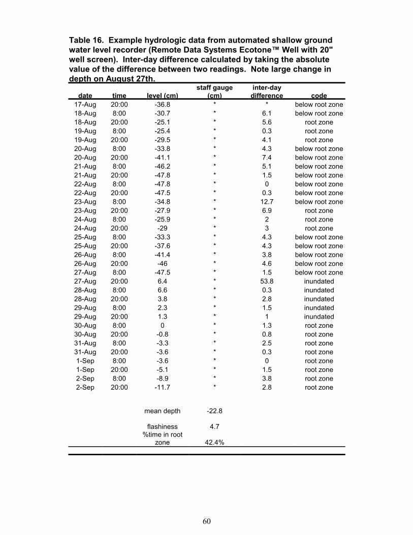
60

Table 16. Example hydrologic data from automated shallow groundwater level recorder (Remote Data Systems Ecotone™ Well with 20"well screen). Inter-day difference calculated by taking the absolutevalue of the difference between two readings. Note large change indepth on August 27th.

date time level (cm)staff gauge

(cm)inter-day

difference code17-Aug 20:00 -36.8 * * below root zone18-Aug 8:00 -30.7 * 6.1 below root zone18-Aug 20:00 -25.1 * 5.6 root zone19-Aug 8:00 -25.4 * 0.3 root zone19-Aug 20:00 -29.5 * 4.1 root zone20-Aug 8:00 -33.8 * 4.3 below root zone20-Aug 20:00 -41.1 * 7.4 below root zone21-Aug 8:00 -46.2 * 5.1 below root zone21-Aug 20:00 -47.8 * 1.5 below root zone22-Aug 8:00 -47.8 * 0 below root zone22-Aug 20:00 -47.5 * 0.3 below root zone23-Aug 8:00 -34.8 * 12.7 below root zone23-Aug 20:00 -27.9 * 6.9 root zone24-Aug 8:00 -25.9 * 2 root zone24-Aug 20:00 -29 * 3 root zone25-Aug 8:00 -33.3 * 4.3 below root zone25-Aug 20:00 -37.6 * 4.3 below root zone26-Aug 8:00 -41.4 * 3.8 below root zone26-Aug 20:00 -46 * 4.6 below root zone27-Aug 8:00 -47.5 * 1.5 below root zone27-Aug 20:00 6.4 * 53.8 inundated28-Aug 8:00 6.6 * 0.3 inundated28-Aug 20:00 3.8 * 2.8 inundated29-Aug 8:00 2.3 * 1.5 inundated29-Aug 20:00 1.3 * 1 inundated30-Aug 8:00 0 * 1.3 root zone30-Aug 20:00 -0.8 * 0.8 root zone31-Aug 8:00 -3.3 * 2.5 root zone31-Aug 20:00 -3.6 * 0.3 root zone1-Sep 8:00 -3.6 * 0 root zone1-Sep 20:00 -5.1 * 1.5 root zone2-Sep 8:00 -8.9 * 3.8 root zone2-Sep 20:00 -11.7 * 2.8 root zone

mean depth -22.8

flashiness 4.7%time in root

zone 42.4%

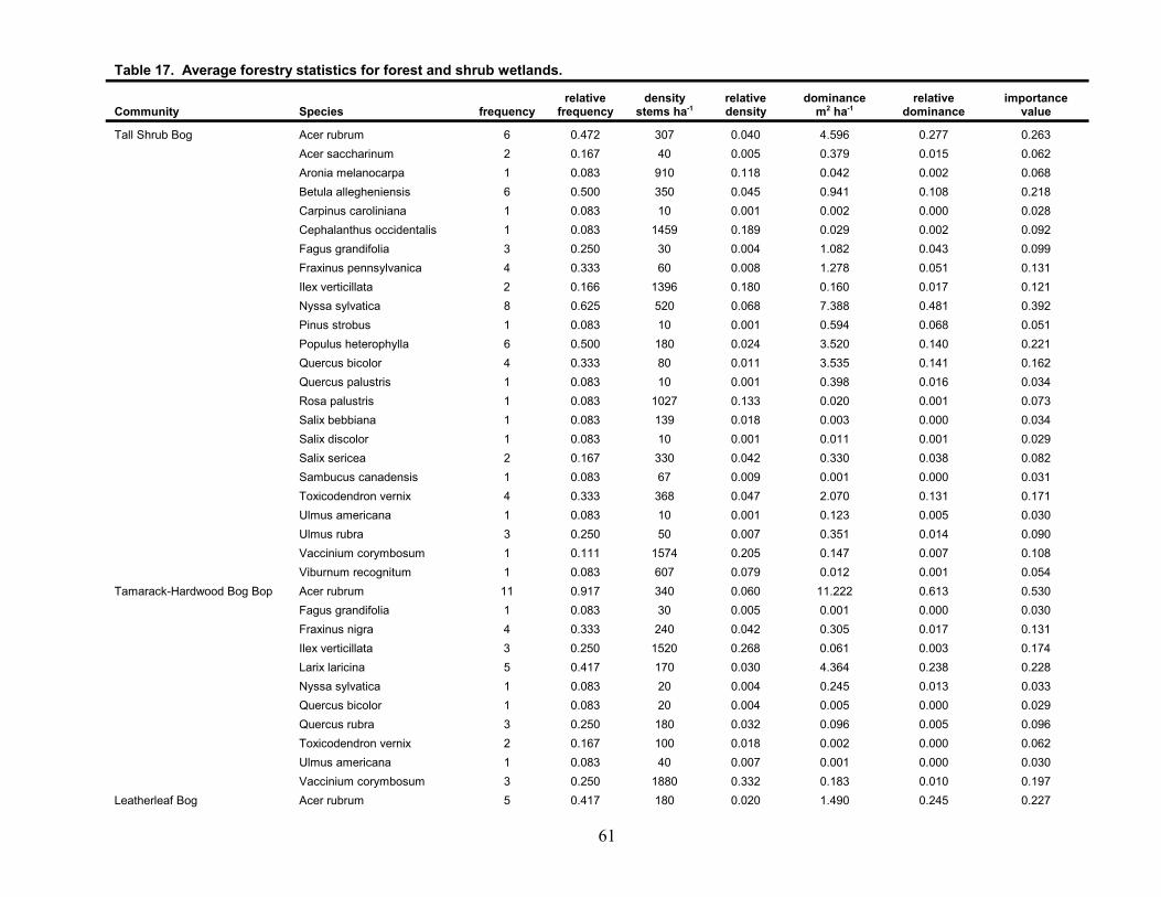
61

Table 17. Average forestry statistics for forest and shrub wetlands.

Community Species frequencyrelative

frequencydensity

stems ha-1relativedensity

dominancem2 ha-1

relativedominance

importancevalue

Tall Shrub Bog Acer rubrum 6 0.472 307 0.040 4.596 0.277 0.263Acer saccharinum 2 0.167 40 0.005 0.379 0.015 0.062Aronia melanocarpa 1 0.083 910 0.118 0.042 0.002 0.068Betula allegheniensis 6 0.500 350 0.045 0.941 0.108 0.218Carpinus caroliniana 1 0.083 10 0.001 0.002 0.000 0.028Cephalanthus occidentalis 1 0.083 1459 0.189 0.029 0.002 0.092Fagus grandifolia 3 0.250 30 0.004 1.082 0.043 0.099Fraxinus pennsylvanica 4 0.333 60 0.008 1.278 0.051 0.131Ilex verticillata 2 0.166 1396 0.180 0.160 0.017 0.121Nyssa sylvatica 8 0.625 520 0.068 7.388 0.481 0.392Pinus strobus 1 0.083 10 0.001 0.594 0.068 0.051Populus heterophylla 6 0.500 180 0.024 3.520 0.140 0.221Quercus bicolor 4 0.333 80 0.011 3.535 0.141 0.162Quercus palustris 1 0.083 10 0.001 0.398 0.016 0.034Rosa palustris 1 0.083 1027 0.133 0.020 0.001 0.073Salix bebbiana 1 0.083 139 0.018 0.003 0.000 0.034Salix discolor 1 0.083 10 0.001 0.011 0.001 0.029Salix sericea 2 0.167 330 0.042 0.330 0.038 0.082Sambucus canadensis 1 0.083 67 0.009 0.001 0.000 0.031Toxicodendron vernix 4 0.333 368 0.047 2.070 0.131 0.171Ulmus americana 1 0.083 10 0.001 0.123 0.005 0.030Ulmus rubra 3 0.250 50 0.007 0.351 0.014 0.090Vaccinium corymbosum 1 0.111 1574 0.205 0.147 0.007 0.108Viburnum recognitum 1 0.083 607 0.079 0.012 0.001 0.054

Tamarack-Hardwood Bog Bop Acer rubrum 11 0.917 340 0.060 11.222 0.613 0.530Fagus grandifolia 1 0.083 30 0.005 0.001 0.000 0.030Fraxinus nigra 4 0.333 240 0.042 0.305 0.017 0.131Ilex verticillata 3 0.250 1520 0.268 0.061 0.003 0.174Larix laricina 5 0.417 170 0.030 4.364 0.238 0.228Nyssa sylvatica 1 0.083 20 0.004 0.245 0.013 0.033Quercus bicolor 1 0.083 20 0.004 0.005 0.000 0.029Quercus rubra 3 0.250 180 0.032 0.096 0.005 0.096Toxicodendron vernix 2 0.167 100 0.018 0.002 0.000 0.062Ulmus americana 1 0.083 40 0.007 0.001 0.000 0.030Vaccinium corymbosum 3 0.250 1880 0.332 0.183 0.010 0.197

Leatherleaf Bog Acer rubrum 5 0.417 180 0.020 1.490 0.245 0.227

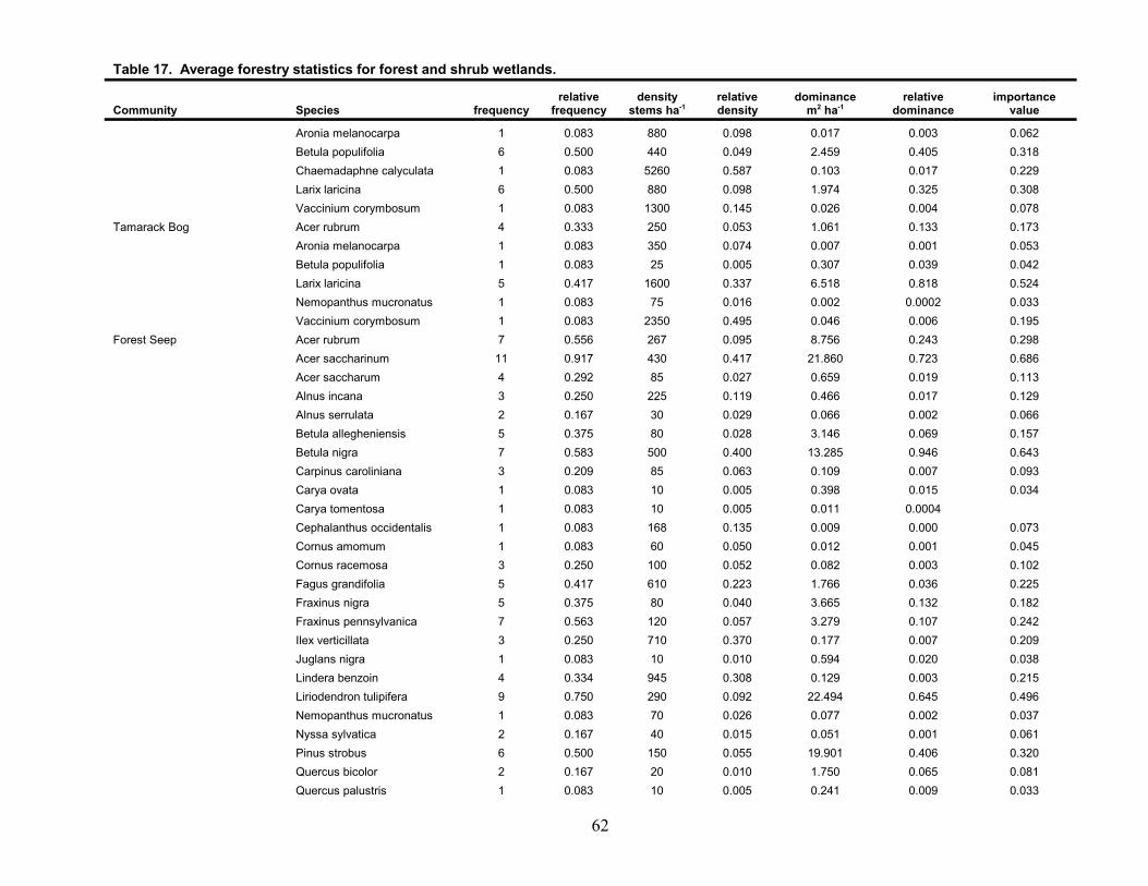
Table 17. Average forestry statistics for forest and shrub wetlands.

Community Species frequencyrelative

frequencydensity

stems ha-1relativedensity

dominancem2 ha-1

relativedominance

importancevalue

62

Aronia melanocarpa 1 0.083 880 0.098 0.017 0.003 0.062Betula populifolia 6 0.500 440 0.049 2.459 0.405 0.318Chaemadaphne calyculata 1 0.083 5260 0.587 0.103 0.017 0.229Larix laricina 6 0.500 880 0.098 1.974 0.325 0.308Vaccinium corymbosum 1 0.083 1300 0.145 0.026 0.004 0.078

Tamarack Bog Acer rubrum 4 0.333 250 0.053 1.061 0.133 0.173Aronia melanocarpa 1 0.083 350 0.074 0.007 0.001 0.053Betula populifolia 1 0.083 25 0.005 0.307 0.039 0.042Larix laricina 5 0.417 1600 0.337 6.518 0.818 0.524Nemopanthus mucronatus 1 0.083 75 0.016 0.002 0.0002 0.033Vaccinium corymbosum 1 0.083 2350 0.495 0.046 0.006 0.195

Forest Seep Acer rubrum 7 0.556 267 0.095 8.756 0.243 0.298Acer saccharinum 11 0.917 430 0.417 21.860 0.723 0.686Acer saccharum 4 0.292 85 0.027 0.659 0.019 0.113Alnus incana 3 0.250 225 0.119 0.466 0.017 0.129Alnus serrulata 2 0.167 30 0.029 0.066 0.002 0.066Betula allegheniensis 5 0.375 80 0.028 3.146 0.069 0.157Betula nigra 7 0.583 500 0.400 13.285 0.946 0.643Carpinus caroliniana 3 0.209 85 0.063 0.109 0.007 0.093Carya ovata 1 0.083 10 0.005 0.398 0.015 0.034Carya tomentosa 1 0.083 10 0.005 0.011 0.0004Cephalanthus occidentalis 1 0.083 168 0.135 0.009 0.000 0.073Cornus amomum 1 0.083 60 0.050 0.012 0.001 0.045Cornus racemosa 3 0.250 100 0.052 0.082 0.003 0.102Fagus grandifolia 5 0.417 610 0.223 1.766 0.036 0.225Fraxinus nigra 5 0.375 80 0.040 3.665 0.132 0.182Fraxinus pennsylvanica 7 0.563 120 0.057 3.279 0.107 0.242Ilex verticillata 3 0.250 710 0.370 0.177 0.007 0.209Juglans nigra 1 0.083 10 0.010 0.594 0.020 0.038Lindera benzoin 4 0.334 945 0.308 0.129 0.003 0.215Liriodendron tulipifera 9 0.750 290 0.092 22.494 0.645 0.496Nemopanthus mucronatus 1 0.083 70 0.026 0.077 0.002 0.037Nyssa sylvatica 2 0.167 40 0.015 0.051 0.001 0.061Pinus strobus 6 0.500 150 0.055 19.901 0.406 0.320Quercus bicolor 2 0.167 20 0.010 1.750 0.065 0.081Quercus palustris 1 0.083 10 0.005 0.241 0.009 0.033

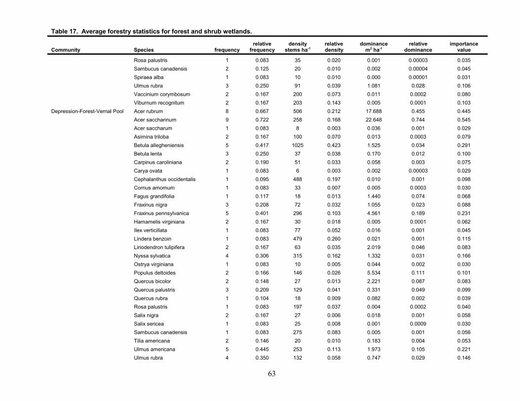
Table 17. Average forestry statistics for forest and shrub wetlands.

Community Species frequencyrelative

frequencydensity

stems ha-1relativedensity

dominancem2 ha-1

relativedominance

importancevalue

63

Rosa palustris 1 0.083 35 0.020 0.001 0.00003 0.035Sambucus canadensis 2 0.125 20 0.010 0.002 0.00004 0.045Spiraea alba 1 0.083 10 0.010 0.000 0.00001 0.031Ulmus rubra 3 0.250 91 0.039 1.081 0.028 0.106Vaccinium corymbosum 2 0.167 200 0.073 0.011 0.0002 0.080Viburnum recognitum 2 0.167 203 0.143 0.005 0.0001 0.103

Depression-Forest-Vernal Pool Acer rubrum 8 0.667 506 0.212 17.688 0.455 0.445Acer saccharinum 9 0.722 258 0.168 22.648 0.744 0.545Acer saccharum 1 0.083 8 0.003 0.036 0.001 0.029Asimina triloba 2 0.167 100 0.070 0.013 0.0003 0.079Betula allegheniensis 5 0.417 1025 0.423 1.525 0.034 0.291Betula lenta 3 0.250 37 0.038 0.170 0.012 0.100Carpinus caroliniana 2 0.190 51 0.033 0.058 0.003 0.075Carya ovata 1 0.083 6 0.003 0.002 0.00003 0.029Cephalanthus occidentalis 1 0.095 488 0.197 0.010 0.001 0.098Cornus amomum 1 0.083 33 0.007 0.005 0.0003 0.030Fagus grandifolia 1 0.117 18 0.013 1.440 0.074 0.068Fraxinus nigra 3 0.208 72 0.032 1.055 0.023 0.088Fraxinus pennsylvanica 5 0.401 296 0.103 4.561 0.189 0.231Hamamelis virginiana 2 0.167 30 0.018 0.005 0.0001 0.062Ilex verticillata 1 0.083 77 0.052 0.016 0.001 0.045Lindera benzoin 1 0.083 479 0.260 0.021 0.001 0.115Liriodendron tulipifera 2 0.167 63 0.035 2.019 0.046 0.083Nyssa sylvatica 4 0.306 315 0.162 1.332 0.031 0.166Ostrya virginiana 1 0.083 10 0.005 0.044 0.002 0.030Populus deltoides 2 0.166 146 0.026 5.534 0.111 0.101Quercus bicolor 2 0.148 27 0.013 2.221 0.087 0.083Quercus palustris 3 0.209 129 0.041 0.331 0.049 0.099Quercus rubra 1 0.104 18 0.009 0.082 0.002 0.039Rosa palustris 1 0.083 197 0.037 0.004 0.0002 0.040Salix nigra 2 0.167 27 0.006 0.018 0.001 0.058Salix sericea 1 0.083 25 0.008 0.001 0.0009 0.030Sambucus canadensis 1 0.083 275 0.083 0.005 0.001 0.056Tilia americana 2 0.146 20 0.010 0.183 0.004 0.053Ulmus americana 5 0.445 253 0.113 1.973 0.105 0.221Ulmus rubra 4 0.350 132 0.058 0.747 0.029 0.146

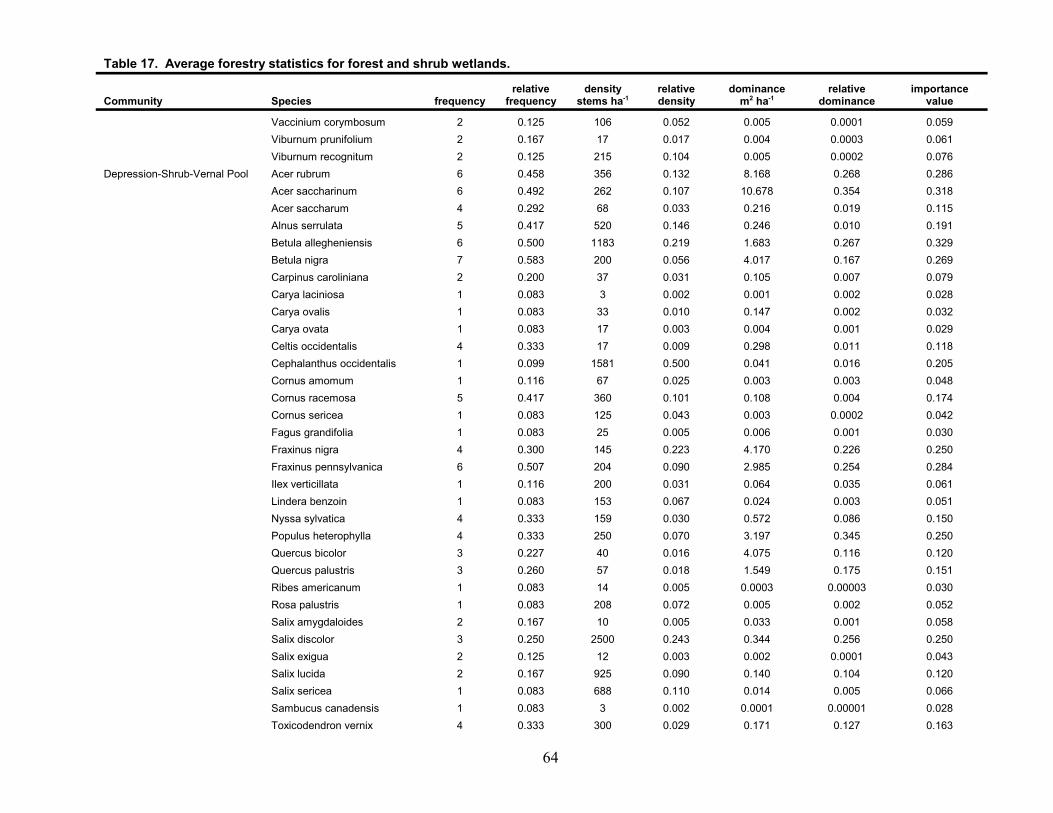
Table 17. Average forestry statistics for forest and shrub wetlands.

Community Species frequencyrelative

frequencydensity

stems ha-1relativedensity

dominancem2 ha-1

relativedominance

importancevalue

64

Vaccinium corymbosum 2 0.125 106 0.052 0.005 0.0001 0.059Viburnum prunifolium 2 0.167 17 0.017 0.004 0.0003 0.061Viburnum recognitum 2 0.125 215 0.104 0.005 0.0002 0.076

Depression-Shrub-Vernal Pool Acer rubrum 6 0.458 356 0.132 8.168 0.268 0.286Acer saccharinum 6 0.492 262 0.107 10.678 0.354 0.318Acer saccharum 4 0.292 68 0.033 0.216 0.019 0.115Alnus serrulata 5 0.417 520 0.146 0.246 0.010 0.191Betula allegheniensis 6 0.500 1183 0.219 1.683 0.267 0.329Betula nigra 7 0.583 200 0.056 4.017 0.167 0.269Carpinus caroliniana 2 0.200 37 0.031 0.105 0.007 0.079Carya laciniosa 1 0.083 3 0.002 0.001 0.002 0.028Carya ovalis 1 0.083 33 0.010 0.147 0.002 0.032Carya ovata 1 0.083 17 0.003 0.004 0.001 0.029Celtis occidentalis 4 0.333 17 0.009 0.298 0.011 0.118Cephalanthus occidentalis 1 0.099 1581 0.500 0.041 0.016 0.205Cornus amomum 1 0.116 67 0.025 0.003 0.003 0.048Cornus racemosa 5 0.417 360 0.101 0.108 0.004 0.174Cornus sericea 1 0.083 125 0.043 0.003 0.0002 0.042Fagus grandifolia 1 0.083 25 0.005 0.006 0.001 0.030Fraxinus nigra 4 0.300 145 0.223 4.170 0.226 0.250Fraxinus pennsylvanica 6 0.507 204 0.090 2.985 0.254 0.284Ilex verticillata 1 0.116 200 0.031 0.064 0.035 0.061Lindera benzoin 1 0.083 153 0.067 0.024 0.003 0.051Nyssa sylvatica 4 0.333 159 0.030 0.572 0.086 0.150Populus heterophylla 4 0.333 250 0.070 3.197 0.345 0.250Quercus bicolor 3 0.227 40 0.016 4.075 0.116 0.120Quercus palustris 3 0.260 57 0.018 1.549 0.175 0.151Ribes americanum 1 0.083 14 0.005 0.0003 0.00003 0.030Rosa palustris 1 0.083 208 0.072 0.005 0.002 0.052Salix amygdaloides 2 0.167 10 0.005 0.033 0.001 0.058Salix discolor 3 0.250 2500 0.243 0.344 0.256 0.250Salix exigua 2 0.125 12 0.003 0.002 0.0001 0.043Salix lucida 2 0.167 925 0.090 0.140 0.104 0.120Salix sericea 1 0.083 688 0.110 0.014 0.005 0.066Sambucus canadensis 1 0.083 3 0.002 0.0001 0.00001 0.028Toxicodendron vernix 4 0.333 300 0.029 0.171 0.127 0.163

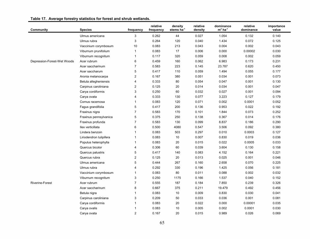
Table 17. Average forestry statistics for forest and shrub wetlands.

Community Species frequencyrelative

frequencydensity

stems ha-1relativedensity

dominancem2 ha-1

relativedominance

importancevalue

65

Ulmus americana 3 0.262 44 0.027 1.054 0.132 0.140Ulmus rubra 3 0.264 120 0.040 1.434 0.072 0.125Vaccinium corymbosum 10 0.083 213 0.043 0.004 0.002 0.043Viburnum prunifolium 1 0.083 17 0.006 0.000 0.00002 0.030Viburnum recognitum 1 0.117 320 0.059 0.008 0.002 0.059

Depression-Forest-Wet Woods Acer rubrum 6 0.459 160 0.062 6.983 0.173 0.231Acer saccharinum 7 0.583 223 0.145 23.787 0.620 0.450Acer saccharum 5 0.417 110 0.059 1.494 0.055 0.177Aronia melanocarpa 2 0.167 380 0.051 0.034 0.001 0.073Betula allegheniensis 4 0.333 80 0.054 0.047 0.001 0.130Carpinus caroliniana 2 0.125 20 0.014 0.034 0.001 0.047Carya cordiformis 3 0.250 60 0.032 0.027 0.001 0.094Carya ovata 4 0.333 130 0.077 3.223 0.127 0.179Cornus racemosa 1 0.083 120 0.071 0.002 0.0001 0.052Fagus grandifolia 5 0.417 200 0.136 0.953 0.022 0.192Fraxinus nigra 7 0.583 170 0.101 1.844 0.073 0.252Fraxinus pennsylvanica 5 0.375 250 0.138 0.367 0.014 0.176Fraxinus profunda 7 0.583 130 0.099 8.837 0.186 0.290Ilex verticillata 6 0.500 4080 0.547 3.506 0.092 0.380Lindera benzoin 1 0.083 503 0.297 0.010 0.0003 0.127Liriodendron tulipifera 1 0.083 10 0.007 0.830 0.019 0.036Populus heterophylla 1 0.083 20 0.015 0.022 0.0005 0.033Quercus bicolor 4 0.306 60 0.039 3.604 0.130 0.158Quercus palustris 5 0.417 140 0.083 4.152 0.164 0.221Quercus rubra 2 0.125 20 0.013 0.025 0.001 0.046Ulmus americana 5 0.444 267 0.160 2.658 0.070 0.225Ulmus rubra 4 0.292 330 0.196 1.425 0.056 0.181Vaccinium corymbosum 1 0.083 80 0.011 0.088 0.002 0.032Viburnum recognitum 3 0.250 1175 0.166 1.537 0.040 0.152

Riverine-Forest Acer rubrum 7 0.555 187 0.184 7.850 0.239 0.326Acer saccharinum 8 0.667 375 0.211 19.479 0.492 0.456Betula nigra 1 0.083 10 0.009 0.830 0.030 0.041Carpinus caroliniana 3 0.209 50 0.033 0.036 0.001 0.081Carya cordiformis 1 0.083 20 0.022 0.000 0.00001 0.035Carya ovalis 1 0.083 10 0.005 0.002 0.0001 0.030Carya ovata 2 0.167 20 0.015 0.989 0.026 0.069

Table 17. Average forestry statistics for forest and shrub wetlands.

Community Species frequencyrelative

frequencydensity

stems ha-1relativedensity

dominancem2 ha-1

relativedominance

importancevalue

66

Cephalanthus occidentalis 1 0.104 463 0.323 0.040 0.001 0.143Cornus sp. 1 0.083 90 0.101 0.002 0.00004 0.062Fraxinus pennsylvanica 8 0.625 325 0.192 6.440 0.161 0.326Ilex verticillata 2 0.125 225 0.294 0.009 0.0003 0.140Lindera benzoin 1 0.111 213 0.163 0.005 0.0001 0.091Populus deltoides 1 0.083 50 0.026 20.402 0.480 0.197Populus heterophylla 2 0.167 40 0.021 0.766 0.018 0.069Quercus bicolor 3 0.208 50 0.067 11.235 0.325 0.200Quercus palustris 3 0.229 68 0.082 12.748 0.329 0.213Ulmus americana 8 0.667 130 0.069 3.255 0.077 0.271Ulmus rubra 3 0.250 63 0.045 0.775 0.021 0.105

Riverine-Shrub Acer rubrum 6 0.500 305 0.122 5.792 0.294 0.305Acer saccharinum 6 0.479 200 0.115 4.970 0.231 0.275Alnus serrulata 3 0.208 658 0.379 0.046 0.007 0.198Betula nigra 4 0.292 211 0.080 2.047 0.165 0.179Celtis occidentalis 1 0.083 10 0.008 0.123 0.004 0.032Cephalanthus occidentalis 1 0.083 1644 0.567 0.032 0.007 0.219Fraxinus pennsylvanica 6 0.472 308 0.186 12.168 0.437 0.365Ilex verticillata 1 0.083 350 0.127 0.007 0.0003 0.070Juglans nigra 1 0.083 10 0.008 0.123 0.004 0.032Quercus palustris 2 0.167 25 0.018 3.087 0.332 0.172Salix nigra 2 0.167 60 0.041 0.839 0.042 0.083Spiraea tomentosa 1 0.083 70 0.033 0.001 0.001 0.039

Ulmus americana 4 0.292 85 0.064 1.457 0.049 0.135Ulmus rubra 1 0.083 13 0.003 0.301 0.014 0.0

23 The following HGM classes should be used: depression, impoundment-human, impoundment-beaver, riverine-headwater, riverine-mainstem, riverine-channel, slope, fringing, coastal, bog (weaklyombrotrophic), bog (moderately-strongly ombrotrophic).

24 The following duration classes should be used: permanently inundated, regularly inundated,seasonally inundated, permanently saturated, regularly saturated, seasonally saturated.

25 The following plant community classes should be used: swamp forest, bog forest, forest seep,marsh, wet meadow-fen, wet meadow-other, sphagnum bog, shrub swamp, tall shrub bog, tall shrub fen.

67

Table 18. Background information on wetland type, location, number, amount, andmonitoring period for wetland mitigation. Insert information for each mitigationwetland required to be constructed.

ImpactedWetland(s)

MitigationWetland(s)

(add columnsas needed)

a. Name of project(s)

b. County where project(s) located

c. Latitude and Longitude of project(s) (DD.DDDDD)

d. Name of watershed(s) where wetland(s) are located

e. 11 and 14 Digit HUC code(s) where wetland(s) located

f. HGM class of the site(s) (Table 1A, 15)23.

g. Duration of inundation/saturation24

List hydroperiod (~%) of each site (e.g. ~30 %seasonallyinundated, ~70% regularly inundated, etc.)

h. Dominant plant community(ies) (Table 1B)25

List plant community (~%), e.g. ~20% marsh, ~80% wetmeadow -fen

I. Ecological region where site(s) will be located (ECBP,EOLP, WAP, IP, MIDP, HELP) (Figure 1)

j. Length of monitoring period in yearsSpecify number of years of monitoring required, e.g. 5, 10,15 etc.

k. Monitoring FrequencySpecify monitoring frequency, e.g. every year (annual),every other year (biennial), every third year (triennial), etc.

l. The number of individual wetland areas that wereimpacted or number of individual mitigation wetlands thatare to be constructed

m. Total acreage of wetlands in hectares (acres)

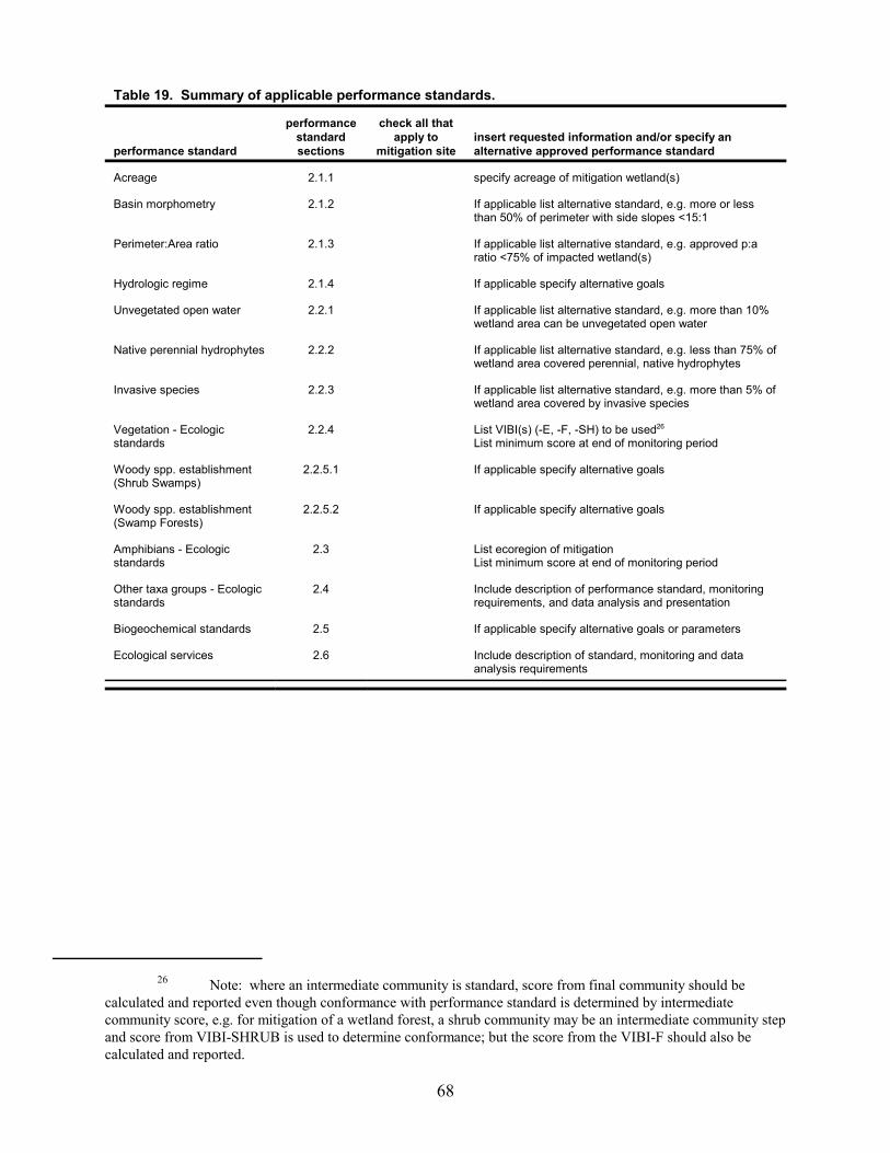
26 Note: where an intermediate community is standard, score from final community should becalculated and reported even though conformance with performance standard is determined by intermediatecommunity score, e.g. for mitigation of a wetland forest, a shrub community may be an intermediate community stepand score from VIBI-SHRUB is used to determine conformance; but the score from the VIBI-F should also becalculated and reported.

68

Table 19. Summary of applicable performance standards.

performance standard

performancestandardsections

check all thatapply to

mitigation siteinsert requested information and/or specify analternative approved performance standard

Acreage 2.1.1 specify acreage of mitigation wetland(s)

Basin morphometry 2.1.2 If applicable list alternative standard, e.g. more or lessthan 50% of perimeter with side slopes <15:1

Perimeter:Area ratio 2.1.3 If applicable list alternative standard, e.g. approved p:aratio <75% of impacted wetland(s)

Hydrologic regime 2.1.4 If applicable specify alternative goals

Unvegetated open water 2.2.1 If applicable list alternative standard, e.g. more than 10%wetland area can be unvegetated open water

Native perennial hydrophytes 2.2.2 If applicable list alternative standard, e.g. less than 75% ofwetland area covered perennial, native hydrophytes

Invasive species 2.2.3 If applicable list alternative standard, e.g. more than 5% ofwetland area covered by invasive species

Vegetation - Ecologicstandards

2.2.4 List VIBI(s) (-E, -F, -SH) to be used26

List minimum score at end of monitoring period

Woody spp. establishment(Shrub Swamps)

2.2.5.1 If applicable specify alternative goals

Woody spp. establishment(Swamp Forests)

2.2.5.2 If applicable specify alternative goals

Amphibians - Ecologicstandards

2.3 List ecoregion of mitigationList minimum score at end of monitoring period

Other taxa groups - Ecologicstandards

2.4 Include description of performance standard, monitoringrequirements, and data analysis and presentation

Biogeochemical standards 2.5 If applicable specify alternative goals or parameters

Ecological services 2.6 Include description of standard, monitoring and dataanalysis requirements

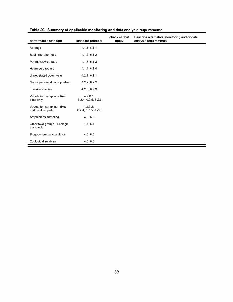
69

Table 20. Summary of applicable monitoring and data analysis requirements.

performance standard standard protocolcheck all that

applyDescribe alternative monitoring and/or dataanalysis requirements

Acreage 4.1.1, 6.1.1

Basin morphometry 4.1.2, 6.1.2

Perimeter:Area ratio 4.1.3, 6.1.3

Hydrologic regime 4.1.4, 6.1.4

Unvegetated open water 4.2.1, 6.2.1

Native perennial hydrophytes 4.2.2, 6.2.2

Invasive species 4.2.3, 6.2.3

Vegetation sampling - fixedplots only

4.2.6.1, 6.2.4, 6.2.5, 6.2.6

Vegetation sampling - fixedand random plots

4.2.6.2, 6.2.4, 6.2.5, 6.2.6

Amphibians sampling 4.3, 6.3

Other taxa groups - Ecologicstandards

4.4, 6.4

Biogeochemical standards 4.5, 6.5

Ecological services 4.6, 6.6

70

Table 21. Generic Credit Release Schedule.

Release of initial20% of credits

Release of next 10%of credits

Release of next 20%of credits

Release of next 20%of credits.

Release of last 20%

Constructioncompleted within 6months of release.

at least 30% of the areaof the mitigation bankmeets wetland criteria

goal HGM class andhydroperiod achieved

at least 90% of thearea of the mitigationbank meets wetlandcriteria

greater than 75% ofarea of mitigationbank vegetated byperennial nativehydrophytes

less than 5% of areaof mitigation bankvegetated by invasivespecies

data shows thatmitigation bank on atrajectory to meetperformancestandards by the endof the monitoringperiod

80% of area ofmitigation bank hasmet all performancestandards or datashows that mitigationbank on a trajectoryto meet performancestandards by the endof the monitoringperiod

last 20% of credits willbe held until allperformance criteriaare met for entire bank

71

Figure 1. Ecoregions of Ohio, Indiana, and neighboring states. The Eastern Corn Belt Plains (ECBP) is Region 55, the Huron-ErieLakes Plains (HELP) is Region 57, the Erie-Ontario Drift and LakesPlains (EOLP) is Region 61, and the Western Allegheny Plateau(WAP) is Region 70. There are also small areas of Region 56(Michigan-Indiana Till Plains) and Region 71 (Interior Plateau) in farnorthwest and southwest Ohio, respectively.

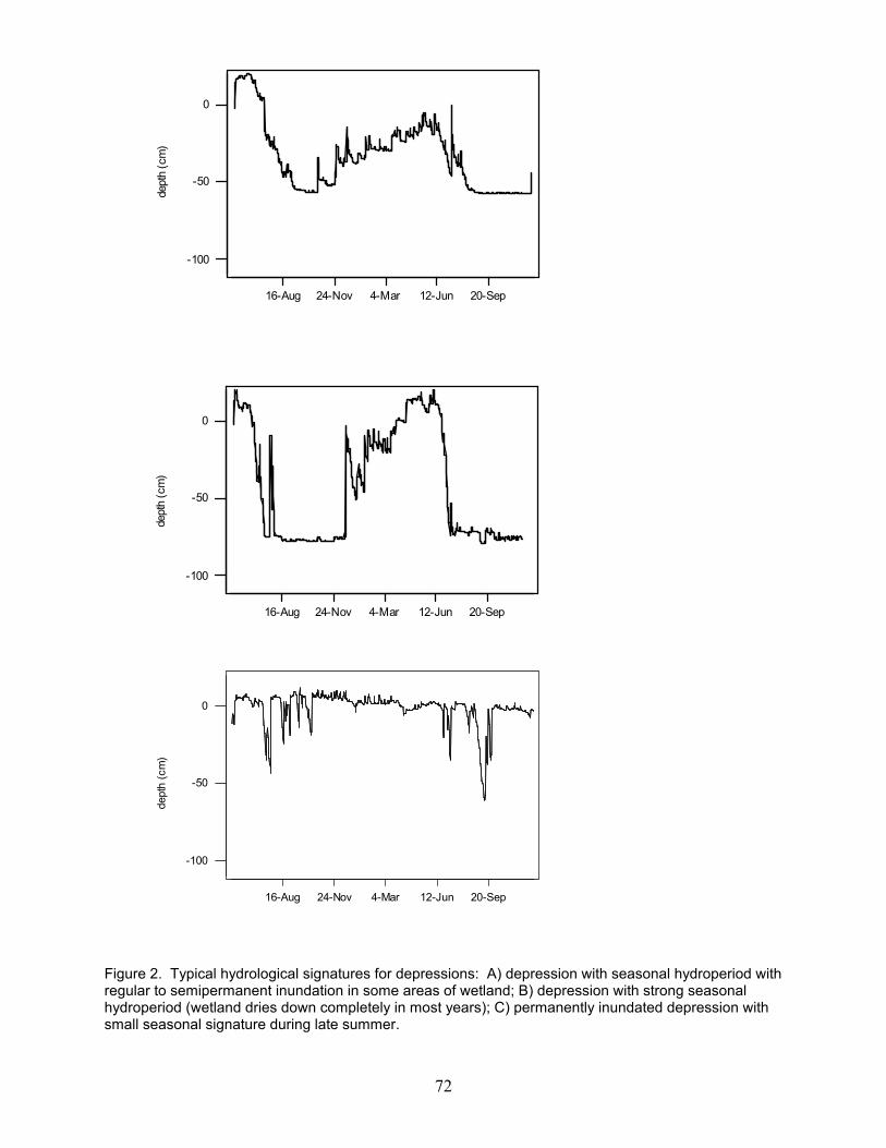
72

16-Aug 24-Nov 4-Mar 12-Jun 20-Sep

-100

-50

0

dept

h (c

m)

20-Sep12-Jun4-Mar24-Nov16-Aug

0

-50

-100

dept

h (c

m)

20-Sep12-Jun4-Mar24-Nov16-Aug

0

-50

-100

dept

h (c

m)

Figure 2. Typical hydrological signatures for depressions: A) depression with seasonal hydroperiod withregular to semipermanent inundation in some areas of wetland; B) depression with strong seasonalhydroperiod (wetland dries down completely in most years); C) permanently inundated depression withsmall seasonal signature during late summer.

73

20-Sep12-Jun4-Mar24-Nov16-Aug

0

-50

-100

dept

h (c

m)

Dec-17Oct-28Sep-8Jul-20

50

0

-50

dept

h (c

m)

Figure 3. Hydrologic signature of an impoundment. Natural beaver pond on floodplain of Eagle Creek. Strong seasonal hydrology with occasional abrupt refilling of wetland.

Figure 4. Hydrologic signature of a two slope wetlands. Upper line is slope wetland with hydrologichead (water is pushed up the well screen above ground level) and permanently saturated conditions(gap in hydrograph is due to data logger damage from deer). Lower line is slope wetland with a moreseasonally saturated hydrology. Note summer decline in ground water inputs with multiple rechargeevents .

74

20-Sep12-Jun4-Mar24-Nov16-Aug

0

-50

-100

dept

h (c

m)

20-Sep12-Jun4-Mar24-Nov16-Aug

0

-50

-100

dept

h (c

m)

Figure 5. Hydrologic signature of riverine wetlands: A) Hydrologic signature of riverine mainstem wetland. Seasonally inundated with occasional flood events during the growing season which partiallyrefill the wetland; B) Hydrologic signature of riverine headwater wetland. Permanently saturated andregularly inundated with ground water input moderating seasonal signature.

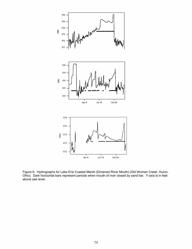
75

Apr-9 Jul-18 Oct-26

571

572

573

574

575

576

1989

Apr-9 Jul-18 Oct-26

572

573

574

575

576

1992

Apr-9 Jul-18 Oct-26

572

573

574

575

576

1994

Figure 6. Hydrographs for Lake Erie Coastal Marsh (Drowned River Mouth) (Old Woman Creek, Huron,Ohio). Dark horizontal bars represent periods when mouth of river closed by sand bar. Y-axis is in feetabove see level.

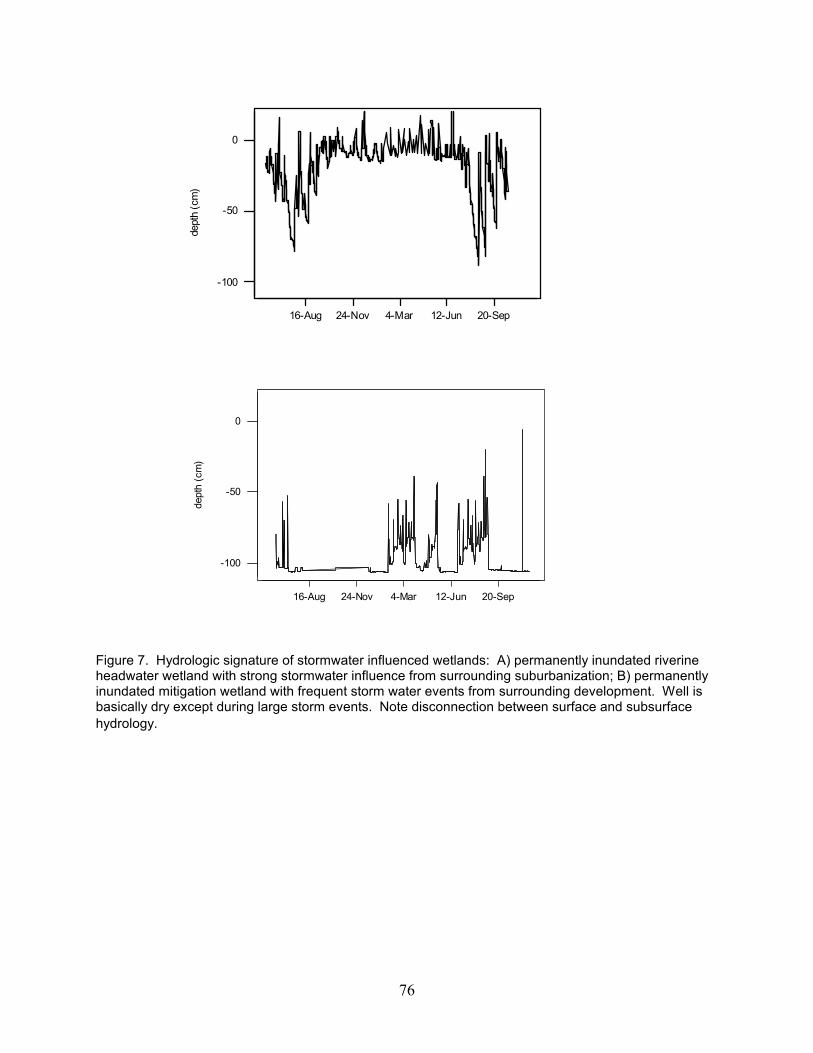
76

20-Sep12-Jun4-Mar24-Nov16-Aug

0

-50

-100

dept

h (c

m)

20-Sep12-Jun4-Mar24-Nov16-Aug

0

-50

-100

dept

h (c

m)

Figure 7. Hydrologic signature of stormwater influenced wetlands: A) permanently inundated riverineheadwater wetland with strong stormwater influence from surrounding suburbanization; B) permanentlyinundated mitigation wetland with frequent storm water events from surrounding development. Well isbasically dry except during large storm events. Note disconnection between surface and subsurfacehydrology.

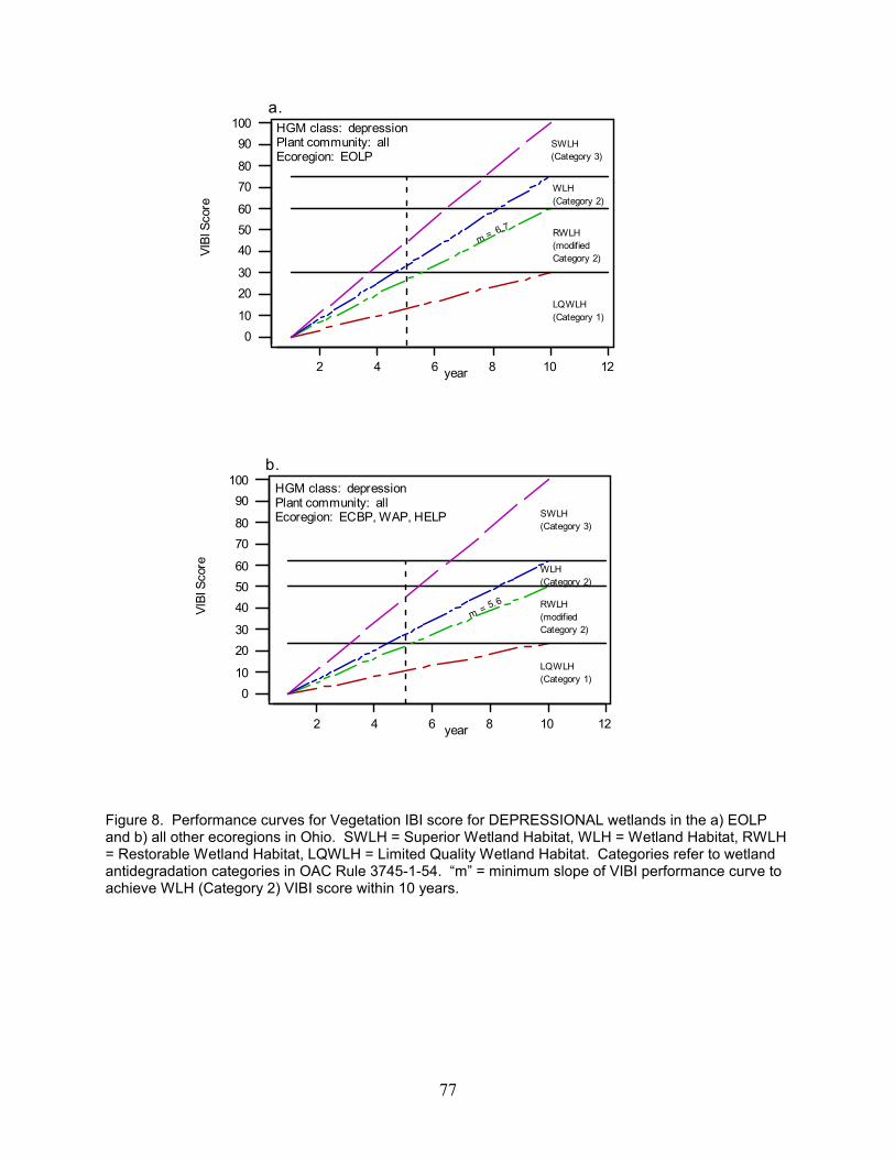
77

12108642

10090

8070

605040

3020

100

year

VIBI

Sco

re

Ecoregion: EOLPPlant community: allHGM class: depression

(Category 1)LQWLH

Category 2)(modifiedRWLH

(Category 2)WLH

(Category 3)SWLH

m = 6.7

a.

12108642

10090

8070

605040

3020

100

year

VIBI

Sco

re

Ecoregion: ECBP, WAP, HELPPlant community: allHGM class: depression

(Category 1)LQWLH

(Category 3)SWLH

(Category 2)WLH

Category 2)(modifiedRWLH

m = 5.6

b.

Figure 8. Performance curves for Vegetation IBI score for DEPRESSIONAL wetlands in the a) EOLPand b) all other ecoregions in Ohio. SWLH = Superior Wetland Habitat, WLH = Wetland Habitat, RWLH= Restorable Wetland Habitat, LQWLH = Limited Quality Wetland Habitat. Categories refer to wetlandantidegradation categories in OAC Rule 3745-1-54. “m” = minimum slope of VIBI performance curve toachieve WLH (Category 2) VIBI score within 10 years.

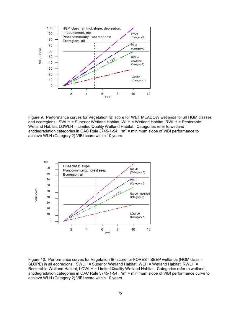
78

12108642

10090

80

70

6050

40

30

2010

0

year

VIB

I Sco

reEcoregion: allPlant community: wet meadowimpoundment, etc.HGM class: all incl. slope, depression,

(Category 1)LQWLH

Category 2)(modifiedRWLH

(Category 2)WLH

(Category 3)SWLH

m = 6.6

2 4 6 8 10 12

0

10

20

30

40

50

60

70

80

90

100

year

VIB

I sco

re

Ecoregion: allPlant community: forest seepHGM class: slope

LQWLH(Category 1)

SWLH(Category 3)

WLH(Category 2)

RWLH (modifiedCategory 2)m = 6.6

Figure 9. Performance curves for Vegetation IBI score for WET MEADOW wetlands for all HGM classesand ecoregions. SWLH = Superior Wetland Habitat, WLH = Wetland Habitat, RWLH = RestorableWetland Habitat, LQWLH = Limited Quality Wetland Habitat. Categories refer to wetlandantidegradation categories in OAC Rule 3745-1-54. “m” = minimum slope of VIBI performance toachieve WLH (Category 2) VIBI score within 10 years.

Figure 10. Performance curves for Vegetation IBI score for FOREST SEEP wetlands (HGM class =SLOPE) in all ecoregions. SWLH = Superior Wetland Habitat, WLH = Wetland Habitat, RWLH =Restorable Wetland Habitat, LQWLH = Limited Quality Wetland Habitat. Categories refer to wetlandantidegradation categories in OAC Rule 3745-1-54. “m” = minimum slope of VIBI performance curve toachieve WLH (Category 2) VIBI score within 10 years.

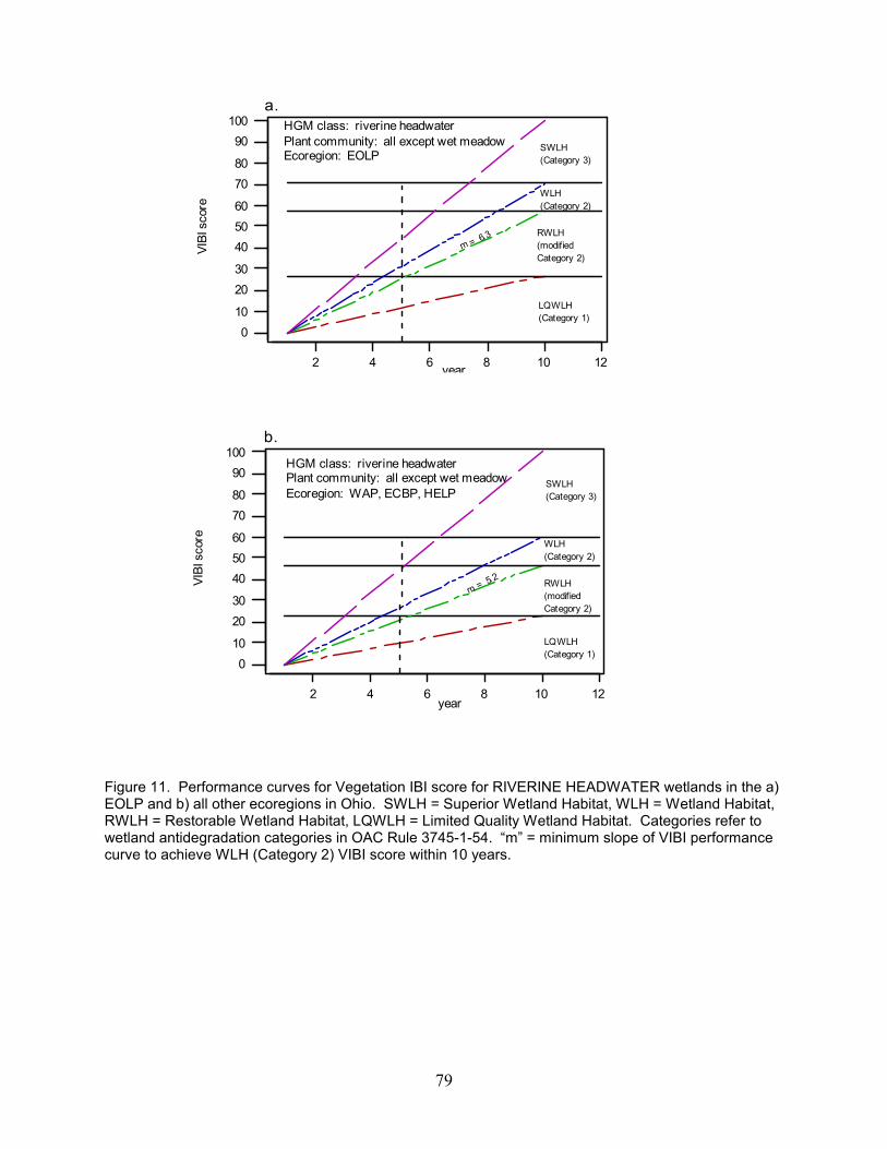
79

2 4 6 8 10 12

010

2030

405060

7080

90100

year

VIBI

sco

re

HGM class: riverine headwaterPlant community: all except wet meadowEcoregion: EOLP

a.

LQWLH(Category 1)

RWLH(modifiedCategory 2)

WLH(Category 2)

SWLH(Category 3)

m = 6.3

12108642

10090

8070

605040

3020

100

year

VIBI

sco

re

Ecoregion: WAP, ECBP, HELPPlant community: all except wet meadowHGM class: riverine headwater

b.

(Category 1)LQWLH

Category 2)(modifiedRWLH

(Category 2)WLH

(Category 3)SWLH

m = 5.2

Figure 11. Performance curves for Vegetation IBI score for RIVERINE HEADWATER wetlands in the a)EOLP and b) all other ecoregions in Ohio. SWLH = Superior Wetland Habitat, WLH = Wetland Habitat,RWLH = Restorable Wetland Habitat, LQWLH = Limited Quality Wetland Habitat. Categories refer towetland antidegradation categories in OAC Rule 3745-1-54. “m” = minimum slope of VIBI performancecurve to achieve WLH (Category 2) VIBI score within 10 years.

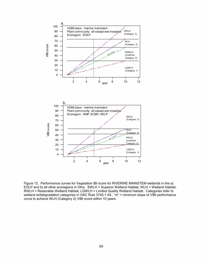
80

12108642

1009080706050

40302010

0

year

VIBI

sco

re

Ecoregion: EOLPPlant community: all except wet meadowHGM class: riverine mainstem

(Category 1)LQWLH

Category 2)(modif iedRQWLH

(Category 2)WLH

(Category 3)SWLH

m = 6.3

a.

2 4 6 8 10 12

010203040

5060708090

100

year

VIBI

sco

re

HGM class: riverine mainstemPlant community: all except wet meadowEcoregion: WAP, ECBP, HELP

m = 4.7

LQWLH(Category 1)

RWLH(modif iedCategory 2)

WLH(Category 2)

SWLH(Category 3)

b.

Figure 12. Performance curves for Vegetation IBI score for RIVERINE MAINSTEM wetlands in the a)EOLP and b) all other ecoregions in Ohio. SWLH = Superior Wetland Habitat, WLH = Wetland Habitat,RWLH = Restorable Wetland Habitat, LQWLH = Limited Quality Wetland Habitat. Categories refer towetland antidegradation categories in OAC Rule 3745-1-54. “m” = minimum slope of VIBI performancecurve to achieve WLH (Category 2) VIBI score within 10 years.

81

2 4 6 8 10 12

010

20

30

40

50

6070

80

90100

year

VIBI

sco

re

HGM class: impoundmentPlant community: marsh, shrub swampEcoregion: EOLP

a.

LQWLH(Category 1)

RWLH(modifiedCategory 2)

WLH(Category 2)

SWLH(Category 3)

m = 6.6

12108642

10090

8070

605040

3020

100

year

VIBI

sco

re

Ecoregion: WAP, ECBP, HELPPlant community: marsh, shrub swampHGM class: impoundment

b.

(Category 1)LQWLH

Category 2)(modifiedRWLH

(Category 2)WLH

(Category 3)SWLH

m = 5.8

Figure 13. Performance curves for Vegetation IBI score for IMPOUNDMENT wetlands in the a) EOLPand b) all other ecoregions in Ohio. SWLH = Superior Wetland Habitat, WLH = Wetland Habitat, RWLH= Restorable Wetland Habitat, LQWLH = Limited Quality Wetland Habitat. Categories refer to wetlandantidegradation categories in OAC Rule 3745-1-54. “m” = minimum slope of VIBI performance curve toachieve WLH (Category 2) VIBI score within 10 years.

82

12108642

10090

8070

605040

3020

100

year

VIBI

sco

re

Ecoregion: all regionsPlant community: tamarack-hardwood, tall shrub bogHGM class: weakly ombrotrophic bog

a.

(Category 1)LQWLH

Category 2)(modifiedRWLH

(Category 2)WLH

(Category 3)SWLH

m = 7.2

12108642

10090

8070

605040

3020

100

year

VIBI

sco

re

Ecoregion: all regionsopen sphagnum bogsPlant community: leatherleaf, tamarack,ombrotrophic bogsHGM class: moderately-strongly

b.

LQWLH

RWLH

WLH

SWLH

m = 2.6

Figure 14. Performance curves for Vegetation IBI score for BOG wetlands in the a) WEAKLYOMBROTROPHIC BOGS b) MODERATELY TO STRONGLY OMBROTROPHIC bogs in all regions. SWLH = Superior Wetland Habitat, WLH = Wetland Habitat, RWLH = Restorable Wetland Habitat,LQWLH = Limited Quality Wetland Habitat. Most bogs are regulated as Category 3 wetlands regardlessof their condition (OAC Rule 3745-1-54). “m” = minimum slope of VIBI performance curve to achieveWLH VIBI score within 10 years.

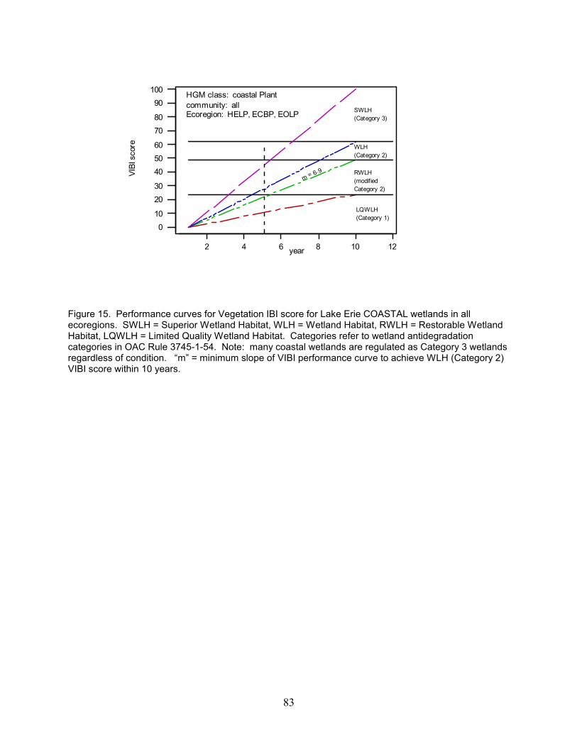
83

12108642

10090

8070

605040

3020

100

year

VIBI

sco

re

Ecoregion: HELP, ECBP, EOLPcommunity: allHGM class: coastal Plant

m = 6.9

(Category 1)LQWLH

Category 2)(modifiedRWLH

(Category 2)WLH

(Category 3)SWLH

Figure 15. Performance curves for Vegetation IBI score for Lake Erie COASTAL wetlands in allecoregions. SWLH = Superior Wetland Habitat, WLH = Wetland Habitat, RWLH = Restorable WetlandHabitat, LQWLH = Limited Quality Wetland Habitat. Categories refer to wetland antidegradationcategories in OAC Rule 3745-1-54. Note: many coastal wetlands are regulated as Category 3 wetlandsregardless of condition. “m” = minimum slope of VIBI performance curve to achieve WLH (Category 2)VIBI score within 10 years.

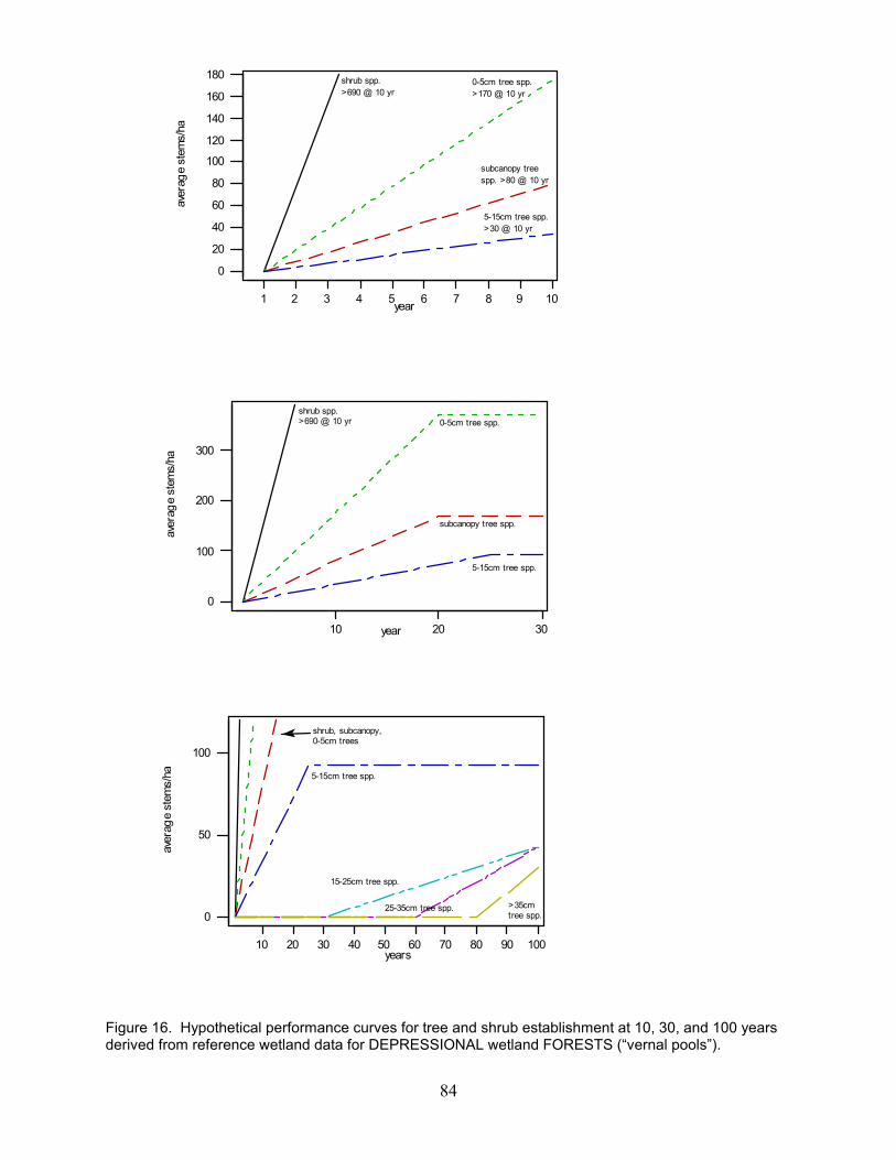
84

100908070605040302010

100

50

0

years

aver

age

stem

s/ha

0-5cm treesshrub, subcanopy,

5-15cm tree spp.

15-25cm tree spp.

25-35cm tree spp.tree spp.>35cm

302010

300

200

100

0

year

aver

age

stem

s/ha

>690 @ 10 yrshrub spp.

0-5cm tree spp.

subcanopy tree spp.

5-15cm tree spp.

10987654321

180

160

140

120

100

80

60

40

20

0

year

aver

age

stem

s/ha

>690 @ 10 yrshrub spp.

>170 @ 10 yr0-5cm tree spp.

spp. >80 @ 10 yrsubcanopy tree

>30 @ 10 yr5-15cm tree spp.

Figure 16. Hypothetical performance curves for tree and shrub establishment at 10, 30, and 100 yearsderived from reference wetland data for DEPRESSIONAL wetland FORESTS (“vernal pools”).

85

302010

200

100

0

years

aver

age

stem

s/ha

>1600 @ 10 yrshrub spp.

0-5cm tree spp.

5-15cm tree spp.

subcanopy tree spp.

100908070605040302010

100

50

0

years

aver

age

stem

s/ha

shrub, 0-5cm trees

5-15cm tree spp.

subcanopy tree spp.

tree spp.15-25cm

tree spp.25-35cm

tree spp.>35cm

10987654321

150

100

50

0

year

aver

age

stem

s/ha

>1600 @ 10 yrshrub spp.

>120 @ 10 yr0-5cm tree spp.

spp. >40 @ 10 yrsubcanopy tree

>30 @ 10 yr5-15cm tree spp.

Figure 17. Hypothetical performance curves for tree and shrub establishment at 10, 30, and 100 yearsderived from reference wetland data for DEPRESSIONAL wetland SHRUB SWAMPS (“vernal pools”).

86

100908070605040302010

90

80

70

60

50

40

30

20

10

0

year

aver

age

stem

s/ha

5-15cm treesshrub, 0-5cm,

subcanopy tree spp.

tree spp.15-25cm

tree spp.25-35cm

tree spp.>35cm

302010

300

200

100

0

year

aver

age

stem

s/ha

>1350 @ 10 yrshrub spp.

0-5cm tree spp.

5-15cm tree spp.

subcanopy tree spp.

10987654321

150

100

50

0

year

aver

age

stem

s/ha

>1350 @ 10 yrshrub spp.

>150 @10 yr0-5cm tree

>150 @10 yr5-15cm tree

>150 @10 yrsubcanopy tree spp.

Figure 18. Hypothetical performance curves for tree and shrub establishment at 10, 30, and 100 yearsderived from reference wetland data for DEPRESSIONAL (flats) wetland FORESTS (“wet woods”).

87

302010

350

300

250

200

150

100

50

0

year

aver

age

stem

s/ha

>1300 @ 10 yrshrub spp.

0-5cm tree spp.

5-15cm tree spp.

subcanopy tree spp.

100908070605040302010

90

80

70

60

50

40

30

20

10

0

year

aver

age

stem

s/ha

0-5cm treesshrub, subcanopy,

5-15cm tree spp.

tree spp.15-25cm

tree spp.25-35cm

tree spp.>35cm

10987654321

150

100

50

0

year

aver

age

stem

s/ha

>1300 @ 10 yrshrub spp.

>150 @ 10 yr0-5cm tree spp.

>50 @ 10 yr5-15cm tree spp.

spp. >15 @ 10 yrsubcanopy tree

Figure 19. Hypothetical performance curves for tree and shrub establishment at 10, 30, and 100 yearsderived from reference wetland data for RIVERINE MAINSTEM wetland FORESTS.

88

100908070605040302010

100

50

0

years

aver

age

stem

s/ha

tree spp.shrub, 0-5cm

5-15cm tree spp.

tree spp.15-25cm

tree spp.25-35cm

tree spp.>35cm

302010

500

400

300

200

100

0

year

aver

age

stem

s/ha

>1250 @10 yrshrub spp.

0-5cm tree spp.

5-15cm tree spp.

10987654321

250

200

150

100

50

0

year

aver

age

stem

s/ha

>1350 @10 yrshrub spp.

>250 @10 yr0-5cm tree

>30 @10 yr5-15cm tree

Figure 20. Hypothetical performance curves for tree and shrub establishment at 10, 30, and 100 yearsderived from reference wetland data for RIVERINE MAINSTEM wetland SHRUB SWAMPS.

89

302010

700

600

500

400

300

200

100

0

year

aver

age

stem

s/ha

shrub spp.

subcanopy tree spp.

0-5cm tree spp.

5-15cm tree spp.

100908070605040302010

100

50

0

year

aver

age

stem

s/ha

0-5cm treessubcanopy,shrub,

5-15cm trees

>35 cm trees25-35cm trees

15-25cm trees

10987654321

10090

8070

605040

3020

100

year

aver

age

stem

s/ha

>700 @10 yrshrub spp.

>30 @10 yr5-15cm trees

>100 @10 yr5-15cm trees

>90 @10 yr0-5cm trees

Figure 21. Hypothetical performance curves for tree and shrub establishment at 10, 30, and 100 yearsderived from reference wetland data for FOREST SEEPS (slope, swamp forests).

90

10 20 30 40 50 60 70 80 90 100

0

50

100

150

year

aver

age

stem

s/ha

5-15cm tree spp.

shrub and 0-5cm tree spp.

15-25cmtree spp.

25-35cmtree spp.

>35cmtree spp.

subcanopy tree spp.

302010

350

300

250

200

150

100

50

0

year

aver

age

stem

s/ha

shrub spp.

0-5cm tree spp.

5-15cm tree spp.

subcanopy tree spp.

10987654321

150

100

50

0

year

aver

age

stem

s/ha

>2600 @ 10 yrshrub spp.

>140 @ 10 yr0-5cm trees

>50 @ 10 yr5-15 cm trees

spp. >5 @ 10 yrsubcanopy tree

Figure 22. Hypothetical performance curves for tree and shrub establishment at 10, 30, and 100 yearsderived from reference wetland data for WEAKLY OMBROTROPHIC BOGS (TALL SHRUB BOG,TAMARACK-HARDWOOD BOG).

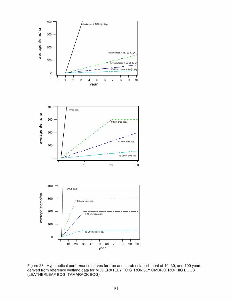
91

0 10 20 30

0

100

200

300

400

year

aver

age

stem

s/ha

shrub spp.

0-5cm tree spp.

15-25cm tree spp.

5-15cm tree spp.

0 10 20 30 40 50 60 70 80 90 100

0

100

200

300

400

year

aver

age

stem

s/ha

shrub spp.

0-5cm tree spp.

5-15cm tree spp.

15-25cm tree spp.

0 1 2 3 4 5 6 7 8 9 10

0

100

200

300

400

year

aver

age

stem

s/ha

shrub spp. >1700 @ 10 yr

0-5cm trees >150 @ 10 yr

5-15cm trees >50 @ 10 yr

15-25cm trees >10 @ 10 yr

Figure 23. Hypothetical performance curves for tree and shrub establishment at 10, 30, and 100 yearsderived from reference wetland data for MODERATELY TO STRONGLY OMBROTROPHIC BOGS(LEATHERLEAF BOG, TAMARACK BOG).

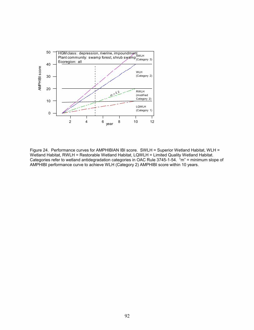
92

12108642

50

40

30

20

10

0

year

AMPH

IBI s

core

Ecoregion: allPlant community: swamp forest, shrub swampHGM class: depression, riverine, impoundment

LQWLH(Category 1)

RWLH(modif iedCategory 2)

WLH(Category 2)

SWLH(Category 3)

m = 2.2

Figure 24. Performance curves for AMPHIBIAN IBI score. SWLH = Superior Wetland Habitat, WLH =Wetland Habitat, RWLH = Restorable Wetland Habitat, LQWLH = Limited Quality Wetland Habitat. Categories refer to wetland antidegradation categories in OAC Rule 3745-1-54. “m” = minimum slope ofAMPHIBI performance curve to achieve WLH (Category 2) AMPHIBI score within 10 years.

93

Figure 25. Typical placement of evenly spaced 15m transects to determine percentage of perimeter withside slopes less than 15:1. In this example, the 3 transects entering the area deeper water have sideslopes greater than 15:1. Therefore, 70% of the wetland perimeter (7/10) is determined to have sideslopes that are greater than 15:1.

Figure 26. Maximum allowable slopes in order to meet 15:1 side slope requirement.

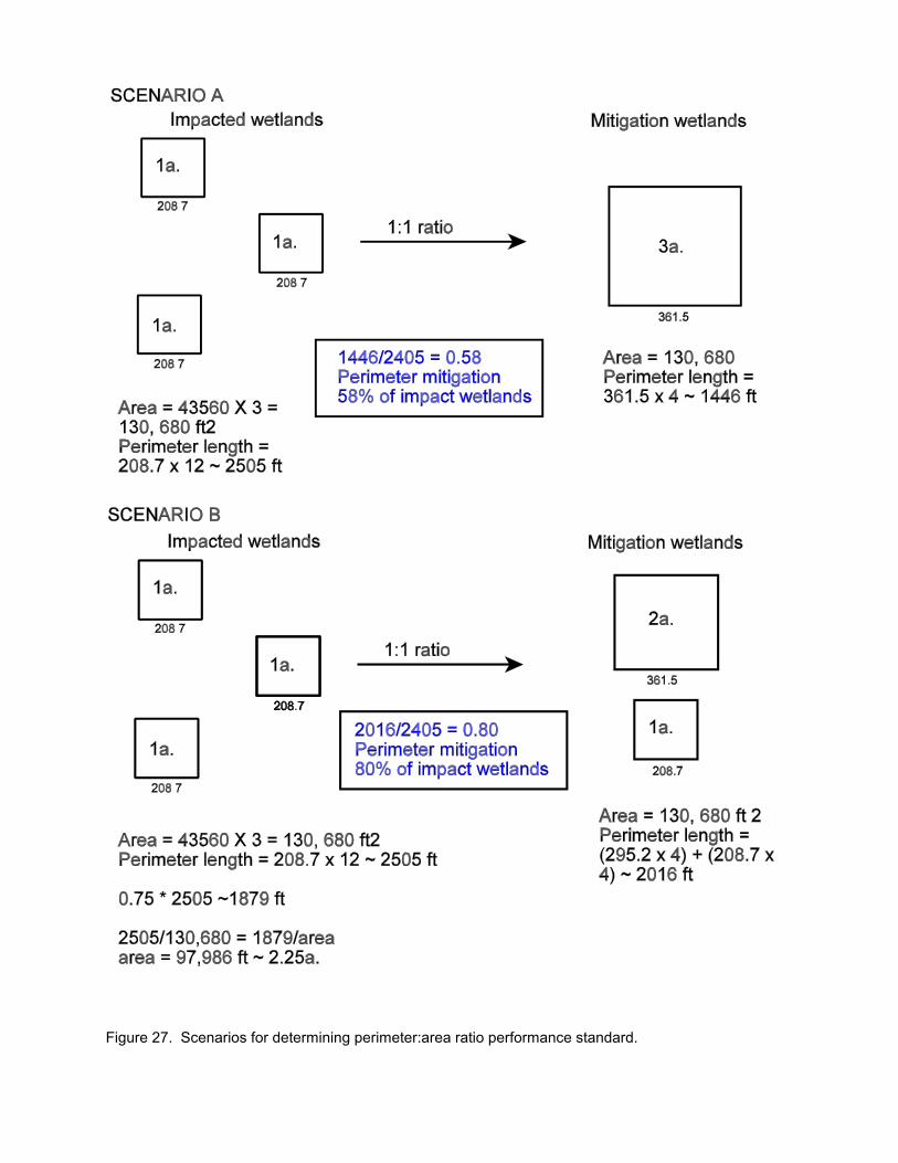
Figure 27. Scenarios for determining perimeter:area ratio performance standard.

96

Figure 28. Mitigation wetland with a predominance of open water and little emergent vegetation. Theintensive modules of a sample plot should focus on the open water with perhaps one end of the plot atthe edge of the wetland.

Figure 29. Mitigation wetland with a some open water and a predominance of emergent vegetation. The intensive modules of a sample plot should focus emergent vegetation with one end of the plotpositioned near the upland edge and the other in an area of deeper water.

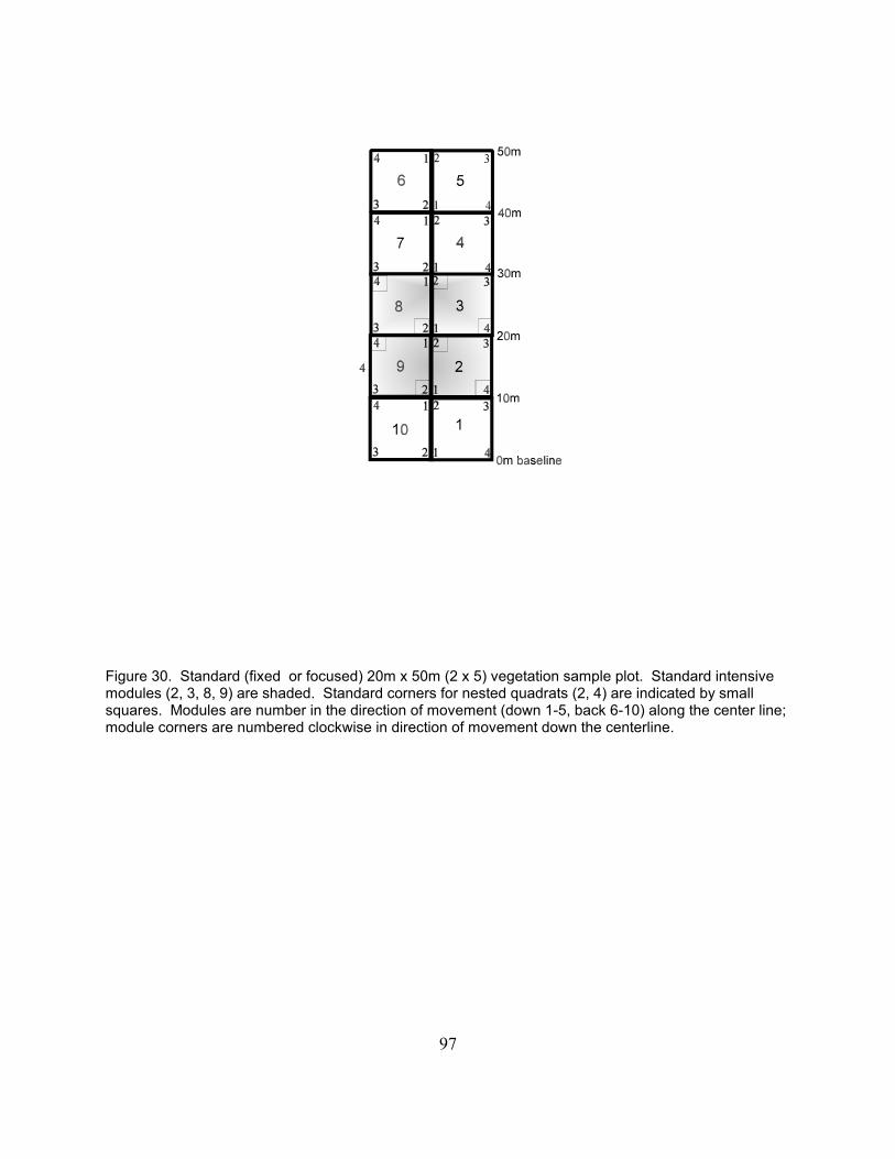
97

Figure 30. Standard (fixed or focused) 20m x 50m (2 x 5) vegetation sample plot. Standard intensivemodules (2, 3, 8, 9) are shaded. Standard corners for nested quadrats (2, 4) are indicated by smallsquares. Modules are number in the direction of movement (down 1-5, back 6-10) along the center line;module corners are numbered clockwise in direction of movement down the centerline.

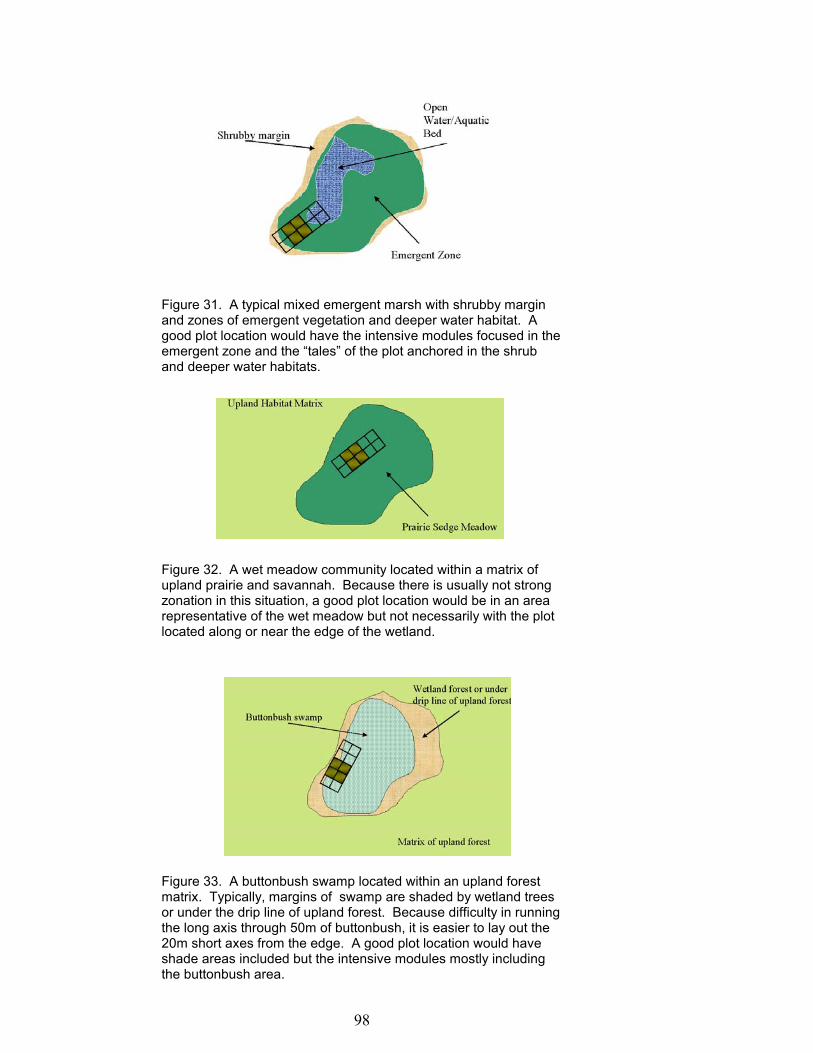
98

Figure 31. A typical mixed emergent marsh with shrubby marginand zones of emergent vegetation and deeper water habitat. Agood plot location would have the intensive modules focused in theemergent zone and the “tales” of the plot anchored in the shruband deeper water habitats.

Figure 32. A wet meadow community located within a matrix ofupland prairie and savannah. Because there is usually not strongzonation in this situation, a good plot location would be in an arearepresentative of the wet meadow but not necessarily with the plotlocated along or near the edge of the wetland.

Figure 33. A buttonbush swamp located within an upland forestmatrix. Typically, margins of swamp are shaded by wetland treesor under the drip line of upland forest. Because difficulty in runningthe long axis through 50m of buttonbush, it is easier to lay out the20m short axes from the edge. A good plot location would haveshade areas included but the intensive modules mostly includingthe buttonbush area.

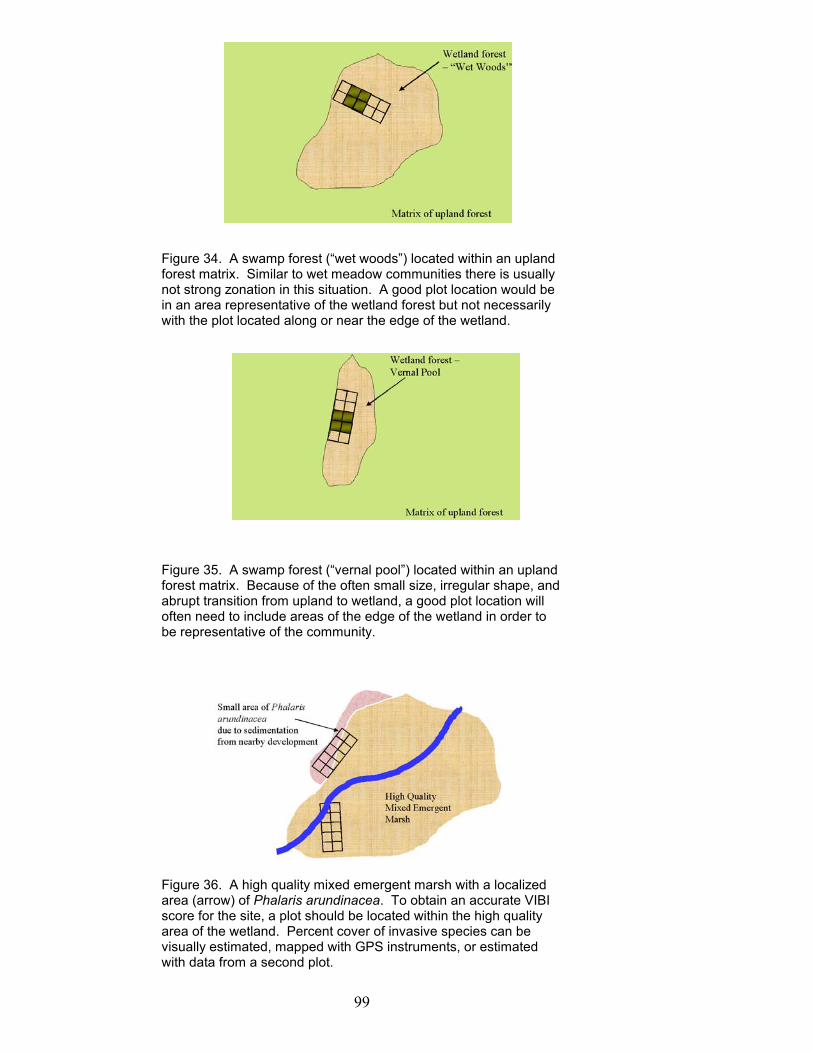
99

Figure 34. A swamp forest (“wet woods”) located within an uplandforest matrix. Similar to wet meadow communities there is usuallynot strong zonation in this situation. A good plot location would bein an area representative of the wetland forest but not necessarilywith the plot located along or near the edge of the wetland.

Figure 35. A swamp forest (“vernal pool”) located within an uplandforest matrix. Because of the often small size, irregular shape, andabrupt transition from upland to wetland, a good plot location willoften need to include areas of the edge of the wetland in order tobe representative of the community.

Figure 36. A high quality mixed emergent marsh with a localizedarea (arrow) of Phalaris arundinacea. To obtain an accurate VIBIscore for the site, a plot should be located within the high qualityarea of the wetland. Percent cover of invasive species can bevisually estimated, mapped with GPS instruments, or estimatedwith data from a second plot.

100

Figure 37. Where a “wetland” is comprised of two HGM classes,separate plots should be established within each HGM class.

Figure 38. Where a wetland is comprised of two co-dominant plantcommunities, separate sample plots should be established in eachcommunity.

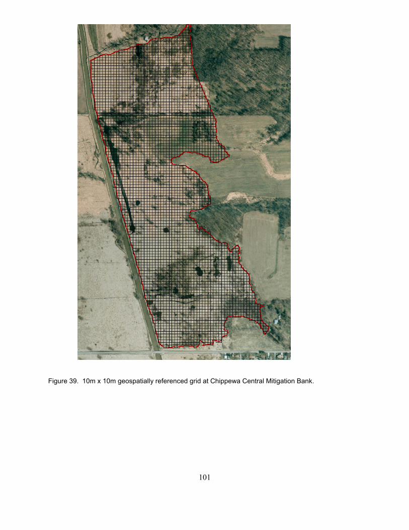
101

Figure 39. 10m x 10m geospatially referenced grid at Chippewa Central Mitigation Bank.

102

Figure 40. Map of random plots at Chippew Central Mitigation Bank. Primary plots are first 20 randomplots which are used first (red); additional 20 plots used (secondary, blue) used if a primary plot is notusable.

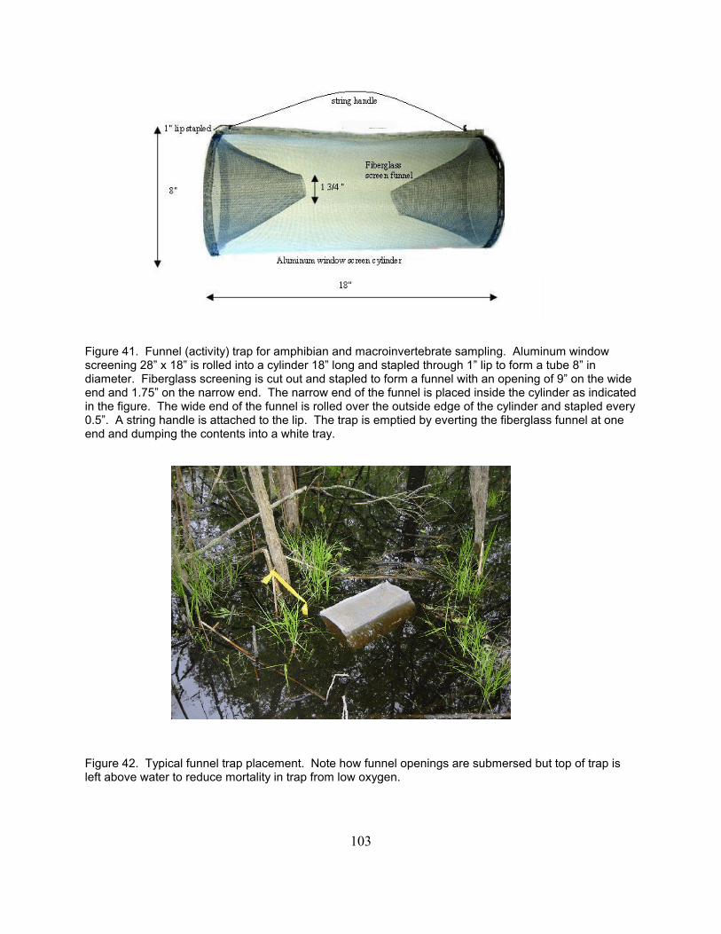
103

Figure 41. Funnel (activity) trap for amphibian and macroinvertebrate sampling. Aluminum windowscreening 28” x 18” is rolled into a cylinder 18” long and stapled through 1” lip to form a tube 8” indiameter. Fiberglass screening is cut out and stapled to form a funnel with an opening of 9” on the wideend and 1.75” on the narrow end. The narrow end of the funnel is placed inside the cylinder as indicatedin the figure. The wide end of the funnel is rolled over the outside edge of the cylinder and stapled every0.5”. A string handle is attached to the lip. The trap is emptied by everting the fiberglass funnel at oneend and dumping the contents into a white tray.

Figure 42. Typical funnel trap placement. Note how funnel openings are submersed but top of trap isleft above water to reduce mortality in trap from low oxygen.

104

x4 x5 Samples 4 and 5: taken half way between the center and the far edge, \ / at a 45 degree angle from initial line (i.e., line made by samples 1 - 3). \ /

x3 Sample 3: taken and the approximate center of the wetland |x2 Sample 2: taken half way between 1 and the approximate center of the wetland |x1 Sample 1: taken approximately 10 m from wetland boundary, near well

Figure 43. Sampling scheme used to collect soil samples at all wetlands.

105

1210

86

42

10 5 0

year

Site D

perf

orm

ance

goa

l

perio

dm

onito

ring

10 y

raf

ter 1

0 yr

sac

tual

trend

regre

ssion

line

year

5 a

nd 9

D.

1210

86

42

10 5 0

year

Site C

perf

orm

ance

goa

l

perio

dm

onito

ring

10 y

r

afte

r 10

yrs

actu

al tre

nd

regre

ssion

line y

ears

5 an

d 9

C.

1210

86

42

10 5 0

year

of m

onito

ring

Site B

perfo

rman

ce g

oal

afte

r 10

yrs

actu

al tr

end

perio

dm

onito

ring

10 yr

regre

ssion

line y

ear 5

and 9

B.

24

68

1012

0510

year

of m

onito

ring

Site A

perfo

rman

ce g

oal

mon

itorin

gpe

riod

regres

sion l

ine y

ear 9

actu

al tr

end

afte

r 10

yrs

regression line year 5

A.

Figu

re 4

4. P

erfo

rman

ce c

urve

sce

nario

s (1

0 ye

ar m

onito

ring

perio

d, d

ata

colle

cted

yea

rs 1

, 3, 5

, 7 9

): A

) Reg

ress

ion

show

s si

teex

ceed

ing

goal

bef

ore

end

of m

onito

ring

perio

d; B

) Site

mee

ts g

oal a

t 10

yrs;

C) R

egre

ssio

n sh

ows

site

mee

ting

goal

by

year

11

(site

cou

ld b

e re

leas

ed fr

om m

onito

ring)

; D) R

egre

ssio

n sh

ows

site

not

mee

ting

goal

by

year

12,

site

per

form

ance

pla

teau

s af

ter

year

7, m

onito

ring

perio

d sh

ould

be

exte

nded

and

cor

rect

ive

actio

n ta

ken.

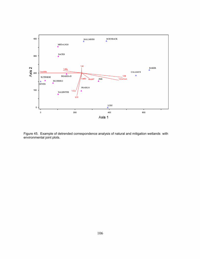
106

Figure 45. Example of detrended correspondence analysis of natural and mitigation wetlands withenvironmental joint plots.