Integrated vehicle control through the coordination of

HAL Id: hal-01509787https://hal.archives-ouvertes.fr/hal-01509787

Submitted on 24 Apr 2017

HAL is a multi-disciplinary open accessarchive for the deposit and dissemination of sci-entific research documents, whether they are pub-lished or not. The documents may come fromteaching and research institutions in France orabroad, or from public or private research centers.

L’archive ouverte pluridisciplinaire HAL, estdestinée au dépôt et à la diffusion de documentsscientifiques de niveau recherche, publiés ou non,émanant des établissements d’enseignement et derecherche français ou étrangers, des laboratoirespublics ou privés.

Integrated vehicle control through the coordination oflongitudinal/lateral and vertical dynamics controllers:

Flatness and LPV/H ∞ based designSoheib Fergani, Lghani Menhour, Olivier Sename, Luc Dugard, Brigitte

d’Andréa-Novel

To cite this version:Soheib Fergani, Lghani Menhour, Olivier Sename, Luc Dugard, Brigitte d’Andréa-Novel. Integratedvehicle control through the coordination of longitudinal/lateral and vertical dynamics controllers:Flatness and LPV/H ∞ based design. International Journal of Robust and Nonlinear Control, Wiley,2017, 27 (18), pp.4992 -5007. 10.1002/rnc.3846. hal-01509787

https://hal.archives-ouvertes.fr/hal-01509787

https://hal.archives-ouvertes.fr

For P

eer Review

INTERNATIONAL JOURNAL OF ROBUST AND NONLINEAR CONTROLInt. J. Robust. Nonlinear Control 2016; 00:1–18Published online in Wiley InterScience (www.interscience.wiley.com). DOI: 10.1002/rnc

Integrated vehicle control through the coordination of

longitudinal/lateral and vertical dynamics controllers:

Flatness and LPV/H∞ based design

S. Fergani1∗, L. Menhour2, O. Sename1, L. Dugard1 and B. D’Andréa-Novel2

1 Institut Supérieur de l’Aéronautique et de l’Espace (ISAE), Toulouse, 31055 France2 Mines-ParisTech, CAOR-Centre de Robotique, Mathématiques et systèmes, France.

SUMMARY

This paper deals with Global Chassis Control (GCC) of ground vehicles. It focuses on the coordinationof suspensions and steering/braking vehicle controllers based on the interaction between the vertical andlateral behaviors of the vehicle. Indeed, the roll motion of the car can generate increasing load transfers thataffect considerably the suspension system and vehicle stability. The load transfers can be described usingthe lateral acceleration. Then, the coordination is highlighted, in this work, through the relationship betweenthe suspension behavior and the lateral acceleration in the framework of the Linear Paramter Varying (LPV)approach.The proposed control law is designed in hierarchical way to improve the overall dynamics of the vehicle.This global control strategy includes two types controllers.The first one is the longitudinal/lateral nonlinear Flatness controller. Based on the adequate choice of theflat outputs, the flatness proof of a 3DoF two wheels nonlinear vehicle model has been established. Then,the combined longitudinal and lateral vehicle control is designed. The algebraic estimation techniques havebeen used in order to have an accuracy estimation of the derivatives and filtering of the reference flat outputs.Such control strategy is developed in order to cope with coupled driving maneuvers like obstacle avoidancevia steering control and stop-and-go control via braking or driving wheel torque.The second part of the proposed strategy consists of the LPV/H∞ suspension controller. This controlleruses the lateral acceleration as a varying parameter to take into account the load transfers that affects directlythe suspension system and therefore to achieve the desired performance.The coordination between the vehicle vertical and lateral dynamics is highlighted in this study, andthe LPV/H∞ framework ensures a specific collaborative coordination between the suspension and thesteering/braking controllers.Simulations on a complex full vehicle model have been validated using experimental data obtained on-boardvehicle, with an identification procedure on a real Renault Mégane Coupé.Copyright c© 2016 John Wiley & Sons, Ltd.

Received . . .

KEY WORDS: Global chassis Control, Braking, Steering, Suspension, LPV, Non linear flatness control,monitoring, H∞, LMI.

Copyright c© 2016 John Wiley & Sons, Ltd.

Prepared using rncauth.cls [Version: 2010/03/27 v2.00]

Page 1 of 19

http://mc.manuscriptcentral.com/rnc-wiley

International Journal of Robust and Nonlinear Control

123456789101112131415161718192021222324252627282930313233343536373839404142434445464748495051525354555657585960

For P

eer Review

2 S. FERGANI

Table I. Variables of Vehicle.

Symbol Variable name UnitVx longitudinal speed [m/s]Vy lateral speed [m/s]ax longitudinal acceleration [m/s2]ay lateral acceleration [m/s2]g gravitational constant [m/s2]µ friction coefficientψ yaw rate [rad/s]ψ yaw angle [rad]φv roll rate [rad/s]φv vehicle roll angle [rad]δ steering angles [rad]Tω braking/traction wheel torque [Nm]Tm engine torque [Nm]Tb braking torque [Nm]

Fyf , Fyr front and rear lateral tire forces [N ]Fszij Suspension verticale forces [N ]αf , αr front and rear tire slip angles [rad]Iz yaw moment of inertia [Kg.m−2]Ix moment of inertia about x axis [kg.m2]Ixz moment of inertia about x and z axes [kg.m2]

m,ms mass and sprung mass of vehicle [Kg]Cf front cornering stiffnesses [N/rad]Cr rear cornering stiffnesses [N/rad]Lf CoG to the front axles distances [m]Lr CoG to the rear axles distances [m]Rω tire radius [m]φr road bank angle [rad]T sampling time [s]

1. NOTATIONS

2. INTRODUCTION

The global chassis control of ground vehicles has been an important issue for the car’s road safetyin the last few years. In the last decade, lots of studies have treated this issue and proposed differentsolutions. Both passive safety systems (airbag, safety belt,...) and active safety systems (ABS,ESP,...) have been widely used by the automotive industry. The use of several actuators on thevehicle have allowed to control the different dynamics of the car, namely, the vertical, the lateral andthe longitudinal ones. Many research works have tried to propose adequate solutions to the vehicledynamics improvement issues, often through the global chassis control involving several actuators.In [1], a new design method of actuator intervention for trajectory tracking is proposed. In [2], aninteresting nonlinear control law using suspension and braking actuators for commercial cars hasbeen developed. Based on the LPV approaches, an integration of steering and braking controllers isproposed in [3], and comments on this integration are given in [4]. More recently, in [5], [6], [7], anLPV control structure that allows to coordinate several actuators and to improve different vehicledynamics has been proposed. However, the suspension control coupled with longitudinal/lateralcontroller remains a challenging problem. Indeed, these problems are usually addressed separately.The proposed strategy is a hierarchical control structure that will improve the overall dynamics ofthe vehicle. It includes two controllers: the first one is the longitudinal/lateral nonlinear Flatnesscontroller. Indeed, many works have proved that the non linear control strategies are efficient to

∗Correspondence to: Département Conception et commande de véhicules AÃ c©ronautiques et Spaciaux (DCAS) InstitutSupérieur de l’Aéronautique et de l’Espace (ISAE), Toulouse, 31055 France. E-mail: [email protected]

Copyright c© 2016 John Wiley & Sons, Ltd. Int. J. Robust. Nonlinear Control (2016)Prepared using rncauth.cls DOI: 10.1002/rnc

Page 2 of 19



123456789101112131415161718192021222324252627282930313233343536373839404142434445464748495051525354555657585960

For P

eer Review

VDC: FLATNESS AND LPV/H∞ BASED DESIGN 3

improve the lateral/longtudinal dynamics of the car. For this sake, the proposed control approachtakes advantage of the flatness property (see [8], [9], [10]) to achieve a global linearization ofthe nonlinear system and of the algebraic estimation techniques for numerical differentiation andfiltering of noisy signals [11], [12], [13]. Moreover, based on the adequate choice of the flat outputs,the flatness proof of a 3DoF two wheels nonlinear vehicle model is established. Thereafter, thecombined longitudinal and lateral vehicle control is designed. The algebraic estimation techniquesare used in order to have an accuracy estimation of the derivatives and filtering of the reference flatoutputs. Such control strategy is developed in order to cope with coupled driving maneuvers likeobstacle avoidance via steering control and stop-and-go control via braking or driving wheel torque.The second part of the proposed strategy consists in the full car LPV/H∞ suspension controller.This controller uses the lateral acceleration as a varying parameter to take into account theload transfers that affects directly the suspension systems and therefore to achieve the desiredperformance. Indeed, the lateral motion of the vehicle is highly correlated to the vertical one throughthe load transfers induced by the roll motions. Based on this correlation, the LPV/H∞ frameworkensures the closed-loop stability for all parameter variations and gets the coordination between thevertical and the lateral dynamics performance objectives.This paper is organized as follows: Section 3 presents the problem formation of the proposedintegration. The design method of flat longitudinal/lateral control is addressed in Section 4. Section 5gives the LPV/H∞ suspension controller and the coordination strategy with flat longitudinal/lateralcontroller. In Section 6, the performance of the proposed integration control strategy are shownthrough simulation results. Finally, conclusions and future work are stated in Section 7.

3. PROBLEM STATEMENT OF THE INTEGRATION OF THE NON LINEAR AND THE LPVCONTROLLERS

The diagram in Fig. 1 describes the integration of the two proposed advanced controllers. In fact, thelateral acceleration controlled with the non linear flatness controller is used to deduce the varyingparameters that schedules the LPV/H∞ suspension controller for the vertical dynamics.The objective of this integrated controller is to improve the vehicle handling and safety. Moreprecisely, the control of longitudinal and lateral motions has a key role to handle some criticalcoupled driving maneuvers such as the obstacle avoidance via steering control. Simultaneously, thepassengers comfort and car roadholding will enhance the vertical dynamics considering the inherentintercorrelation with the lateral ones. Therefore, the coordination in between the 3 main dynamicsof the vehicle is established to achieve the desired performance objectives.It is worth noting that since we are mainly interested by the load transfers caused by the rolldynamics generated, the following relationship between the vertical and lateral dynamics of thevehicle is considered:

θ =zdeffl

− zdeffr+ zdefrl − zdefrrtf

−msayh

kt(1)

where θ: is the roll motion of the vehicle, ay is the lateral acceleration (more details on therelationship between the vertical and the lateral dynamics are given in the following sections),zdefij : is the suspension deflections (i: front or rear, j: left or right), kt : is the tire stiffness.On the other hand, the lateral and the vertical dynamics of the vehicle are correlated through thelateral and vertical tire forces as, (see [14] for more details):

Fiy(βi) = Sign(βi)Fizµ(βi) (2)

where i: is the index for front and rear wheels, Fiy: is the lateral force, βi : is the sideslip, Fiz:is the vertical force and µ(βi): is the road friction. Furthermore, this relationship can be observedalso in the load transfer depending on the roll dynamic and the lateral acceleration ay (notice that


Page 3 of 19



123456789101112131415161718192021222324252627282930313233343536373839404142434445464748495051525354555657585960

For P

eer Review

4 S. FERGANI

Figure 1. Diagram block of the integration strategy

Fy = msayK, where K: is a constant coefficient) as follows,(see [15]):

∆Fz =(

Fzfl+ Fzrl − Fzfr

− Fzrr)

=(

msfl+msrl −mfr −msrr

)

2S1gθ + 2S2ayms/l(3)

where S1 =kftf

+ krtr, S2 =

lfh

tf+ lrh

tr. It is clear that the load transfer generated by the vehicle

bounce are largely influenced by the dynamics of the lateral acceleration, since, as emphasised in(1) the roll motion is also directly linked to ay.Based on the lateral acceleration, the following scheduling parameter is proposed as:

ρa =

∣

∣

∣

∣

ayaymax

∣

∣

∣

∣

(4)

The proposed strategy aims at enhancing the vehicle dynamics by applying, on the full non linearmodel of the vehicle, two kind of controllers acting simultaneously on the vertical dynamics (theLinear Parameters Varying control) and on the lateral/longitudinal dynamics (the non linear Flatnessbased control). An integration of these two control laws is achieved trough the existing correlationsbetween the vehicle vertical, lateral and longitudinal dynamics.

4. FLATNESS-BASED NONLINEAR CONTROL

In this section, the design of the non linear longitudinal/lateral flatness control is described. Thecontroller design structure is summarized in Fig. 2. This scheme summarizes the flatness controldesign structure. The non linear Flatness controller KFlat uses the longitudinal velocity vx, thelateral velocity vy and the yaw rate ψ as inputs. It provides the braking torques Tb and the correctivesteering angle δ+ that stabilize the vehicle in several driving situations.


Page 4 of 19



123456789101112131415161718192021222324252627282930313233343536373839404142434445464748495051525354555657585960

For P

eer Review


Figure 2. Diagram block of the nonlinear flat control

4.1. Nonlinear Vehicle Models for control and simulations

The flatness-based longitudinal/lateral control design is achieved using the three degrees of freedomtwo wheels nonlinear model (3DoF-NLTWVM), given as follows:

msax = ms(Vx − ψVy) = (Fx1 + Fx2)

msay = ms(Vy + ψVx) = (Fy1 + Fy2)

Izψ =Mz1 +Mz2

(5)

where Fxi: the longitudinal forces, Fyi : the lateral forces. The 3DoF single-track nonlinear model

(5) provides a good approximation of the longitudinal, lateral and yaw dynamics. Then, after somemanipulations † of the equations in (5), the following nonlinear equations governing this model areobtained:

x = f(x, t) + g(x)u+ g1u1u2 + g2u22 (6)

where x =

VxVyψ

, u =

[

u1u2

]

, f(x, t) =

ψVy −IrmsR

(ωr + ωf )

−ψVx +1ms

(

−Cf

(

Vy+Lf ψ

Vx

)

− Cr

(

Vy−Lrψ

Vx

))

1Iz

(

−LfCf

(

Vy+Lf ψ

Vx

)

+ LrCr

(

Vy−Lrψ

Vx

))

and g(x, t) =

1msR

Cf

ms

(

Vy+Lf ψ

Vx

)

0 (CfR− Irωf )/msR

0 (LfCfR− LfIrωf )/IzR

.

where the longitudinal motion is controlled via the wheels torques u1 = Tiω = Tim − Tib ,where Tim = 0 (no traction is considered here) and Tib the braking torque for each wheel, and thelateral motion is controlled via the corrective steering angle u2 = δ+. The second order terms u1u2and u22 are neglected because of their small magnitude. More details on the previously used model

†See [16] for details on these models.


Page 5 of 19



123456789101112131415161718192021222324252627282930313233343536373839404142434445464748495051525354555657585960

For P

eer Review

6 S. FERGANI

can be found in [16], [17].For more details see 8.

4.2. Synthesis of the Flatness-based longitudinal/lateral control

Despite these simplifications some coupled behaviors are kept as shown by the functions f(x, t) andg(x, t). Eq. (6) becomes

x = f(x, t) + g(x, t)u (7)

Let us remind that the differential flatness approach of nonlinear systems in a differential algebraiccontext was introduced in [8], [9], [10]. Indeed, the necessary information to run the dynamicbehavior of a real system are easily expressed by the appropriate flat outputs. Numerous engineeringreal applications using flat systems are already handled in the literature (see [9], [10], [18], [19]).Such an approach is also used to manage the coupled nonlinear vehicle control [20], [17] andunderwater vehicles [21] (More application examples of the flatness approach can be found in [22],[23]).Here, since it is well adapted to tracking control problems, the flatness approach is used to dealwith a combined control of longitudinal and lateral vehicle motions using braking on each wheel.The following design problem and flatness property are used to establish the flatness of a 3DoFnonlinear vehicle model. Subsequently, the main objective of this section is presented.

Theorem 1

The following outputs:

y1 = Vx

y2 = LfmsVy − Izψ(8)

are flat outputs for the system (7) (details in [19]).

Remark 1

The first flat output y1 is the longitudinal speed and the second one y2 is the angular momentum ofa point on the axis between the centers of the front and rear axles.

Proof

The flatness control is established thanks to the following flatness property [10], [22].The objective is to show the flatness of model (7) with outputs (8) according to the flatness property37. Then, after some algebraic manipulations we obtain:

x =

VxVyψ

= A(y1, y2, y2)

=

y1

y2L1ms

−(

IzL1ms

)(

L1msy1y2+Cr(L1+L2)y2Cr(L1+L2)(Iz−L2L1ms)+(L1msy1)2

)

−(

L1msy1y2+Cr(L1+L2)y2Cr(L1+L2)(Iz−L2L1ms)+(L1msy1)2

)

(9)

and[

y1y2

]

= ∆(y1, y2, y2)

(

u1u2

)

+Φ(y1, y2, y2) (10)

where

∆ =

[

∆11 ∆12

∆21 ∆22

]

(11)


Page 6 of 19



123456789101112131415161718192021222324252627282930313233343536373839404142434445464748495051525354555657585960

For P

eer Review


and

Φ =

[

Φ1

Φ2

]

(12)

which is equivalent to[

u1u2

]

= ∆−1(y1, y2, y2)

([

y1y2

]

− Φ(y1, y2, y2)

)

(13)

For details concerning ∆ and Φ, see [17]. Thus, the control inputs of the considered systems can bewritten as follows:

u =

[

Tωδ

]

= B(y1, y1, y2, y2, y2)

= ∆−1(y1, y2, y2)

([

y1y2

]

− Φ(y1, y2, y2)

)

(14)

with rx = 1 and ru = 2. Finally, the system (6) is flat system with outputs (8), then, the outputs (8)are called flat outputs.Then, in order to track the desired outputs yref1 and yref2 , the outputs are rewritten as follows:

[

y1y2

]

=

[

yref1 +K11ey1 +K2

1

∫

ey1dt

yref2 +K12ey2 +K2

2

∫

ey2dt+K32 ey2

]

(15)

where, ey1 = yref1 − y1 = V refx − Vx and ey2 = yref2 − y2. The choice of the gain parameters K11 ,

K21 , K

12 , K

22 and K3

2 is then straightforward.

4.3. Algebraic nonlinear estimation

It should be pointed out that the control law (14) contains derivatives of reference signals which arecomputed from measurements such as V refx , V refy , ψref and the derivatives of the measured frontand rear rotational speed wheels ωf and ωr. In order to minimize the effect of the noise on thesederivatives, the numerical differentiation based on an algebraic nonlinear estimation ‡ is proposed.This estimation is performed using the recent advances in [11], [12], which yield efficient real-timefilters §. The following formulae (see, e.g., [26]) may be used:

• Denoising:

y(t) =2!

T 2

∫ t

t−T

(2T − 3τ)y(τ)dτ (16)

• The numerical differentiation of a noisy signal:

ˆy(t) = −3!

T 3

∫ t

t−T

(T − 2τ)y(τ)dτ (17)

Note that the sliding time window [t− T, t] may be quite short.The equations (18) and (19) illustrate the derivatives and filtering of longitudinal speed, lateralspeed, yaw rate and wheels rotation speeds. The results of this application are used as referencesignals in the different parts of the control strategy in (20).

‡See [19], [24], [25] for previous successful applications to intelligent transportation systems.§The above estimation methods are not of asymptotic type and do not require any statistical knowledge of the corruptingnoises (see [13] for details).


Page 7 of 19



123456789101112131415161718192021222324252627282930313233343536373839404142434445464748495051525354555657585960

For P

eer Review

8 S. FERGANI

• The estimated derivatives ˆV refx , ˆV refy , ˆψref , ˆωf and ˆωr are performed as follows:

ˆV refx

ˆV refy

ˆψref

ˆωfˆωr

= −3!

T 3

∫ t

t−T

(2T (t− τ)− T )

V refx

V refy

ψref

ωfωr

dτ (18)

• The filtering ˆV refx , ˆV refy and ˆψref are performed as follows:

V refx

V refy

ˆψref

=

2!

T 2

∫ t

t−T

(3(t− τ)− T )y(τ)

V refx

V refy

ψref

dτ (19)

Finally, the equation of the coupled nonlinear control obtained from equations (14), (15) is asfollows:

u =

[

Tωδ

]

= ∆−1(y1, y2, y2)

(

−Φ(y1, y2, y2) +

[

ˆyref1 +K11 ey1 +K2

1

∫

ey1dt

ˆyref2 +K12 ey2 +K2

2

∫

ey2dt+K32ˆey2

]) (20)

where eyi : are the outputs errors estimations.

5. LPV/H∞ BASED SUSPENSION CONTROL

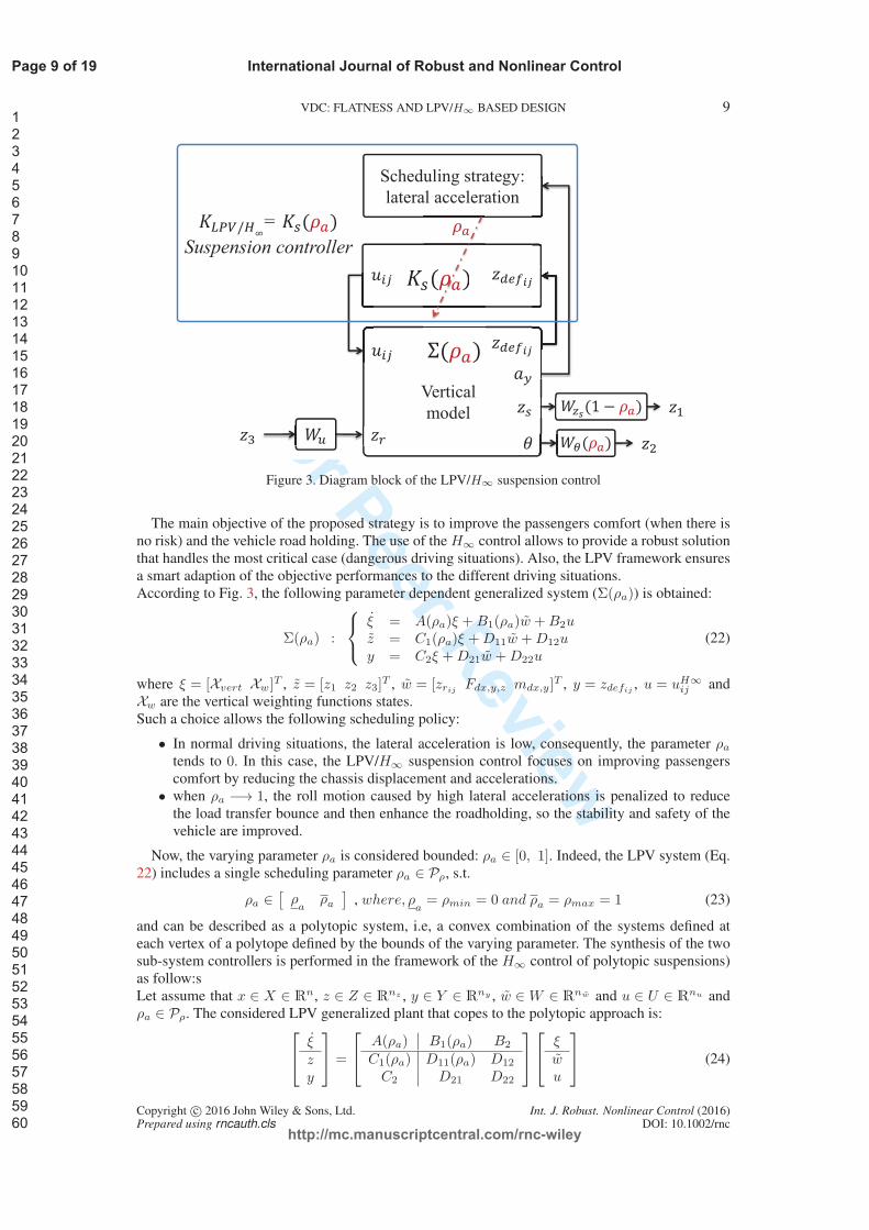
The LPV/H∞ suspension control shown on Fig. 3 is designed using a 7DoF vehicle model (21). Itincludes the following dynamics like: chassis acceleration zs, four wheels accelerations zusij , roll

bounce acceleration θ, pitch acceleration φ.The equations describing the vertical 7DOF model are giving as follows:

zs = −(

Fszf + Fszr + Fdz)

/ms

zusij =(

Fszij − Ftzij)

/musij

θ =(

(Fszrl − Fszrr ) tr +(

Fszfl− Fszfr

)

tf +mshVy)

/Ixφ =

(

Fszf lf − Fszr lr −mshVx)

/Iy

(21)

5.1. LPV/H∞ suspension controller design

The suspension control design aims at providing the performance adaptation thanks to the previouslydefined varying parameter ρa in Section. 4. It is presented in the framework of the H∞ controlapproach including the parameter varying weighting functions and is summarized as follows:

Indeed, according to the control scheme proposed in Fig. 3, let us define:

• Wzs = (1− ρa)s2+2ξ11Ω11s+Ω2

11

s2+2ξ12Ω12s+Ω2

12

is selected to reduce the bounce amplification of the

suspended mass motion (zs) between [0, 12]Hz.

• Wθ = (ρa)s2+2ξ21Ω21s+Ω2

21

s2+2ξ22Ω22s+Ω2

22

which attenuates the roll bounce amplification in low frequencies.

• Wu = 3.10−2 which limits the control signal.

Remark 2

It should be noticed that the parameters of these weighting functions are obtained using geneticalgorithm optimization as in [27].


Page 8 of 19



123456789101112131415161718192021222324252627282930313233343536373839404142434445464748495051525354555657585960

For P

eer Review


Vertical

model

Scheduling strategy:

lateral acceleration

=

Suspension controller

Figure 3. Diagram block of the LPV/H∞ suspension control

The main objective of the proposed strategy is to improve the passengers comfort (when there isno risk) and the vehicle road holding. The use of theH∞ control allows to provide a robust solutionthat handles the most critical case (dangerous driving situations). Also, the LPV framework ensuresa smart adaption of the objective performances to the different driving situations.According to Fig. 3, the following parameter dependent generalized system (Σ(ρa)) is obtained:

Σ(ρa) :

ξ = A(ρa)ξ +B1(ρa)w +B2uz = C1(ρa)ξ +D11w +D12uy = C2ξ +D21w +D22u

(22)

where ξ = [Xvert Xw]T , z = [z1 z2 z3]

T , w = [zrij Fdx,y,z mdx,y]T , y = zdefij , u = uH∞ij and

Xw are the vertical weighting functions states.Such a choice allows the following scheduling policy:

• In normal driving situations, the lateral acceleration is low, consequently, the parameter ρatends to 0. In this case, the LPV/H∞ suspension control focuses on improving passengerscomfort by reducing the chassis displacement and accelerations.

• when ρa −→ 1, the roll motion caused by high lateral accelerations is penalized to reducethe load transfer bounce and then enhance the roadholding, so the stability and safety of thevehicle are improved.

Now, the varying parameter ρa is considered bounded: ρa ∈ [0, 1]. Indeed, the LPV system (Eq.22) includes a single scheduling parameter ρa ∈ Pρ, s.t.

ρa ∈[

ρa

ρa]

, where, ρa= ρmin = 0 and ρa = ρmax = 1 (23)

and can be described as a polytopic system, i.e, a convex combination of the systems defined ateach vertex of a polytope defined by the bounds of the varying parameter. The synthesis of the twosub-system controllers is performed in the framework of the H∞ control of polytopic suspensions)as follow:sLet assume that x ∈ X ∈ Rn, z ∈ Z ∈ Rnz , y ∈ Y ∈ Rny , w ∈W ∈ Rnw and u ∈ U ∈ Rnu andρa ∈ Pρ. The considered LPV generalized plant that copes to the polytopic approach is:

ξzy

=

A(ρa) B1(ρa) B2

C1(ρa) D11(ρa) D12

C2 D21 D22

ξwu

(24)


Page 9 of 19



123456789101112131415161718192021222324252627282930313233343536373839404142434445464748495051525354555657585960

For P

eer Review

10 S. FERGANI

According to this general plant formulation, the LPV controller Ks(ρa) designed is defined as,[

xcu

]

=

[

Ac(ρa) Bc(ρa)Cc(ρa) Dc(ρa)

] [

xcy

]

(25)

where xc ∈ Xc ∈ Rn are the controller states, u ∈ U ∈ Rnu , y ∈ Y ∈ Rny .

According to the varying parameter ρa ∈ Pρ ∈ Rl, the reconstruction of the LPV polytopiccontroller, composed by 2 vertices (see [27]), can be expressed as:

K(ρa) =

2∑

i=1

αi(α)

[

Aci BciCci Dci

]

(26)

where ci define the controller at each vertex of the parameter polytope and where,

αi(ρa) :=

∏2k=1 |ρk − C(ωi)k|∏2k=1(ρk − ρk)

, i = 1, . . . , N (27)

αi(ρa) ≥ 0 and2∑

i=1

αi(ρa) = 1 (28)

Remark 3

It is worth to stress that the use of only one varying parameter reduce the conservatism of theconsidered controller and the make it easy to implement the proposed.

6. SIMULATION RESULTS OF THE INTEGRATED STRATEGY

In this section, we present the simulation results obtained with integrated¶ controller andconsidering a nonlinear vehicle model including vertical and suspension model (more details in[28].

Remark 4

It is worth reminding that the simulation model was validated by experimental tests andimplementations on a real vehicle, the Renault Mégane Coupé (more details in [29]). All the controldesign model are driven (linearization) based on that validated model.

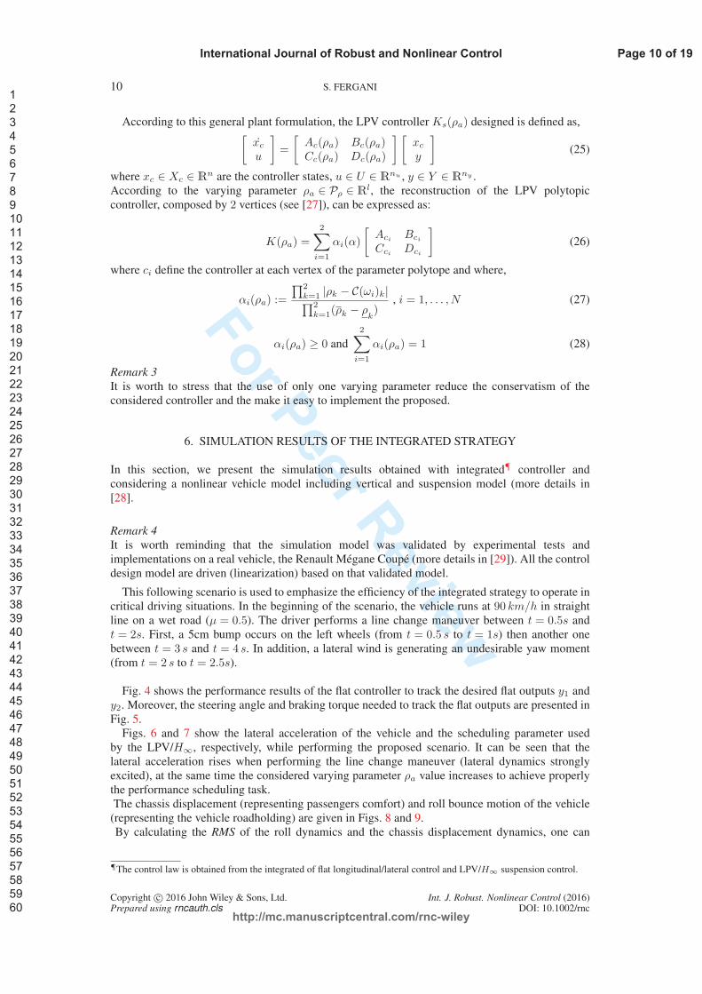
This following scenario is used to emphasize the efficiency of the integrated strategy to operate incritical driving situations. In the beginning of the scenario, the vehicle runs at 90 km/h in straightline on a wet road (µ = 0.5). The driver performs a line change maneuver between t = 0.5s andt = 2s. First, a 5cm bump occurs on the left wheels (from t = 0.5 s to t = 1s) then another onebetween t = 3 s and t = 4 s. In addition, a lateral wind is generating an undesirable yaw moment(from t = 2 s to t = 2.5s).

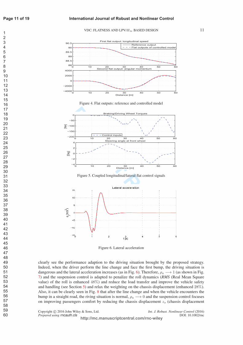
Fig. 4 shows the performance results of the flat controller to track the desired flat outputs y1 andy2. Moreover, the steering angle and braking torque needed to track the flat outputs are presented inFig. 5.

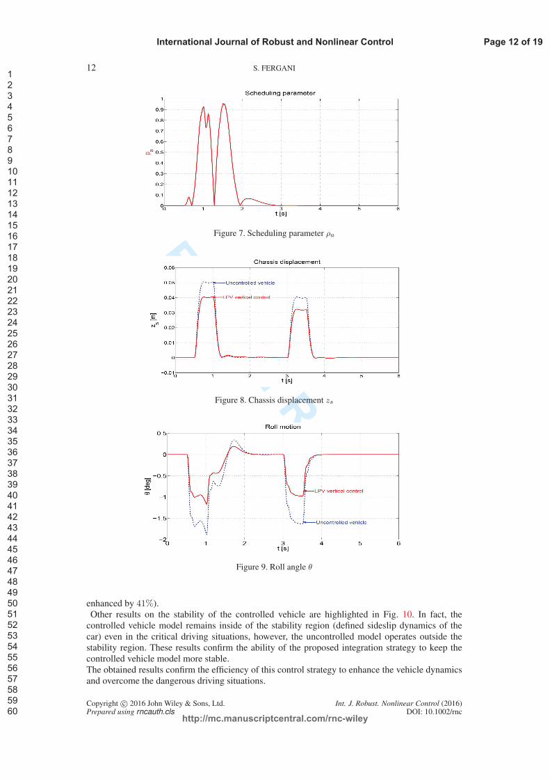
Figs. 6 and 7 show the lateral acceleration of the vehicle and the scheduling parameter usedby the LPV/H∞, respectively, while performing the proposed scenario. It can be seen that thelateral acceleration rises when performing the line change maneuver (lateral dynamics stronglyexcited), at the same time the considered varying parameter ρa value increases to achieve properlythe performance scheduling task.The chassis displacement (representing passengers comfort) and roll bounce motion of the vehicle(representing the vehicle roadholding) are given in Figs. 8 and 9.By calculating the RMS of the roll dynamics and the chassis displacement dynamics, one can

¶The control law is obtained from the integrated of flat longitudinal/lateral control and LPV/H∞ suspension control.


Page 10 of 19



123456789101112131415161718192021222324252627282930313233343536373839404142434445464748495051525354555657585960

For P

eer Review


0 10 20 30 40 50 6088

88.5

89

89.5

90

90.5First flat output: longitudinal speed

Reference output

Flat outputs of controlled model

0 10 20 30 40 50 60−4000

−2000

0

2000

4000Second flat output: angular momentum

Distance [m]

Figure 4. Flat outputs: reference and controlled model

0 10 20 30 40 50 60−200

−150

−100

−50

0

[Nm

]

Braking/Driving Wheel Torques

Control inputs

0 10 20 30 40 50 60−4

−2

0

2

4Steering angle at front wheel

Distance [m]

[Deg

]

Figure 5. Coupled longitudinal/lateral flat control signals

Figure 6. Lateral acceleration

clearly see the performance adaption to the driving situation brought by the proposed strategy.Indeed, when the driver perform the line change and face the first bump, the driving situation isdangerous and the lateral acceleration increases (as in Fig. 6). Therefore, ρa −→ 1 (as shown in Fig.7) and the suspension control is adapted to penalize the roll dynamics (RMS (Real Mean Squarevalue) of the roll is enhanced 48%) and reduce the load transfer and improve the vehicle safetyand handling (see Section 5) and relax the weighting on the chassis displacement (enhanced 28%).Also, it can be clearly seen in Fig. 8 that after the line change and when the vehicle encounters thebump in a straight road, the riving situation is normal, ρa −→ 0 and the suspension control focuseson improving passengers comfort by reducing the chassis displacement zs (chassis displacement


Page 11 of 19



123456789101112131415161718192021222324252627282930313233343536373839404142434445464748495051525354555657585960

For P

eer Review

12 S. FERGANI

Figure 7. Scheduling parameter ρa

Figure 8. Chassis displacement zs

Figure 9. Roll angle θ

enhanced by 41%).Other results on the stability of the controlled vehicle are highlighted in Fig. 10. In fact, thecontrolled vehicle model remains inside of the stability region (defined sideslip dynamics of thecar) even in the critical driving situations, however, the uncontrolled model operates outside thestability region. These results confirm the ability of the proposed integration strategy to keep thecontrolled vehicle model more stable.The obtained results confirm the efficiency of this control strategy to enhance the vehicle dynamicsand overcome the dangerous driving situations.


Page 12 of 19



123456789101112131415161718192021222324252627282930313233343536373839404142434445464748495051525354555657585960

For P

eer Review


−8 −6 −4 −2 0 2 4 6 8−60

−40

−20

0

20

40

60Stability criteria on the vehicle sideslip motion

Side

slip

ang

ular

vel

ocity

[deg

/s]

Sideslip angle [deg]

Stability boundaries of sideslip motion

Controlled Model

Uncontrolled

Stability region

Instability region

Instability region

Limits of the stability region

Figure 10. Stability criteria of sideslip motion: controlled and uncontrolled vehicle models

7. CONCLUSION

In this study, a novel integration strategy of two advanced vehicle controllers is developed. Firstly,the lateral/longitudinal flatness control and the LPV/H∞ vertical dynamics control have beendesigned respectively. Then, an innovative coordination method between the two strategies has beenproposed to establish the collaborative work of the two controllers. This integration aims to improvethe handling and safety of the vehicle, and simultaneously ensures a control coordination of theseveral vehicle dynamics to perform combined maneuvers.Simulation results asses the performance of this collaborative strategy for enhancing thelongitudinal, lateral and vertical dynamics and have shown the efficiency of the proposed approach.Also, using the LPV coordination framework allows to simplify the implementation procedure.


Page 13 of 19



123456789101112131415161718192021222324252627282930313233343536373839404142434445464748495051525354555657585960

For P

eer Review

14 S. FERGANI

8. APPENDIX. RECALL ON FLATNESS BASED ALGEBRAIC THEORY

The idea of differentially flat systems appeared at the nineties of the last century. Flat systems arean important subclass of nonlinear control systems introduced via differential-algebraic methods,defined in a differential geometric framework.The concept of differential algebra is used to define the flat systems, as introduced in [9] and laterusing Lie-Bäcklund transformations. Indeed, the system is said to be flat if one can find a set of

variables, called the flat outputs, such that the system is (non-differentially) algebraic over the

differential field generated by the set of flat outputs. It means that a system is flat if we can find a set

of outputs, such that all states and inputs can be determined from these outputs without integration.

Differentially Flat systems are useful in situations where explicit trajectory generation is required.

Since the behavior of Flat system is determined by the Flat outputs (as previously defined), we can

plan trajectories in output space, and then map them to appropriate inputs. On the other hand, while

this technique is quite powerful, the application differential algebraic results to systems with strong

geometric structure while at the same time exploiting that structure remains a difficult issue without

simplifications.

In the following, some theoretical recalls on the differential flatness control and estimation to better

understand the collaborative work achieved with our colleagues from "Mines-Paritech".

8.1. Basic definitions

Definition 1 (Flat system)

For continuous-time systems, differential flatness is defined as follows. Let us Consider the system:

x = f(x, u) (29)

where x = (x, · · · , xn) ∈ Rn and u = (u, · · · , um) ∈ R

m. It is said to be differentially flat (see [8],

[9], [10] and [22], [23]) if, and only if:

• there exists a vector-valued function h such that

y = h(x, u, u, · · · , u(r)) (30)

where y = (y, · · · , ym) ∈ Rm, r ∈ N;

• the components of x = (x, · · · , xn) and u = (u, · · · , um) may be expressed as

x = A(y, y, · · · , y(rx)), rx ∈ N (31)

u = B(y, y, · · · , y(ru)), ru ∈ N (32)

Remember that y in Eq. (37) is called a flat output.

Remark 5

It is worth noticing that given a flat system, the number of components of a flat output is equal to

the number of independent inputs.

Also, let us recall some properties of the flat systems, that may be useful in the following work

(proofs can be found easily in [22]):

• A flat system is locally reachable.

• A linear system is flat if and only if it is controllable.

• Every flat system is endogenous dynamic feedback linearizable. Conversely, every

endogenous dynamic feedback linearizable system is Flat.

In this study, the flatness property is used for both control and estimation purposes. Indeed, in

the following thesis works, the algebraic estimation is used in this thesis study for the road profile

estimation.


Page 14 of 19



123456789101112131415161718192021222324252627282930313233343536373839404142434445464748495051525354555657585960

For P

eer Review


8.2. A short summary on the algebraic observer

The estimation method uses the algebraic framework devoted for the design of algebraic observers

with unknown inputs [30], [31], [32], [33]. The estimation approach uses also the algebraic

identification methods for the numerical differentiation of noisy signals [32], [12]. The estimation

with unknown input is based on the following properties:

Definition 2

[30], [31]

Consider the following nonlinear model:

x(t) = f(x(t), u(t))y(t) = h(x(t))

(33)

where x(t) is the state vector, u(t) is the input, y(t) is a smooth output and f is continuously

differentiable and f(0; 0) = 0. For the following, we assume that the input u(t) and the output y(t)are continuously differentiable for all t ≥ 0.

The model (33) is said to be algebraically observable if there exist the integers n1 > 0 and n2 > 0such that

x(t) = Γ(

y, y, · · · , y(n1), u, u, · · · , u(n2))

(t) (34)

where Γ(t) is a differentiable real-valued function of the outputs y(t), the inputs u(t), and their

derivatives.

Definition 3

[32], [33]

An unknown input (or a fault) fa is said to be diagnosable if it is possible to estimate the unknown

input fa from the measured outputs of the system. It means in other words that the unknown input

fa is diagnosable if it is algebraically observable, i.e, in general

P (f, u, u, · · · , y, y, · · · ) = 0 (35)

then, the reconstructor (35) can may be used to estimate the unknown input (or a fault) f .

Proposition 1

the algebraic observability of any nonlinear system with unknown inputs is equivalent to express the

dynamical state and the unknown inputs as functions of the inputs, the measured outputs and their

finite time derivatives.

Proposition 2

A system is said observable with unknown inputs if, any state variable or an input variable, can be

formulated as a function of the output and their finite time derivatives. This function can be called

as an input-free estimator. It means in other words that an input-output system is observable with

unknown input if, and only if, its zero dynamics is trivial. In addition, if the system is square, then

the system is called flat ‖ system with its flat output.

Property 1

Consider the system

x = f(x, u) (36)

where x = (x, · · · , xn) ∈ Rn and u = (u, · · · , um) ∈ R

m. It is said to be differentially flat (see [8],

[9], [10] and [22], [23]) if, and only if:

‖The differential flatness property of nonlinear systems in a differential algebraic context was introduced by [9], [10],[22],[23]


Page 15 of 19



123456789101112131415161718192021222324252627282930313233343536373839404142434445464748495051525354555657585960

For P

eer Review

16 S. FERGANI

• there exists a vector-valued function h such that

y = h(x, u, u, · · · , u(r)) (37)

where y = (y, · · · , ym) ∈ Rm, r ∈ N;

• the components of x = (x, · · · , xn) and u = (u, · · · , um) may be expressed as

x = A(y, y, · · · , y(rx)), rx ∈ N (38)

u = B(y, y, · · · , y(ru)), ru ∈ N (39)

Remember that y in Eq. (37) is called a flat output.

The above properties are equivalent to previously presented definitions .

8.3. A short definition of algebraic denoising and numerical differentiation

The numerical estimators ∗∗ (43) are deduced from operational calculation and algebraic

manipulations. For this, consider the following real-valued polynomial time function xN (t) ∈ R[t]of degree N

xN (t) =

N∑

ν=0

x(ν)(0)tν

ν!, t ≥ 0. (40)

In the operational domain †† (see e.g. [34]), (40) becomes

XN (s) =

N∑

ν=0

x(ν)(0)

sν+1. (41)

Multiplying the left-side and the right-side of equation (41) on the left by dα

dsαsN+1, α =

0, 1, · · · , N . The quantities x(ν)(0), ν = 0, 1, . . . , N , which are linearly identifiable satisfy the

following triangular system of linear equations:

dαsN+1XN

dsα=

dα

dsα

(

N∑

ν=0

x(ν)(0)sN−ν

)

, 0 ≤ α ≤ N − 1. (42)

The time derivatives in (42) (sµ dιXN

dsι, µ = 1, . . . , N , 0 ≤ ι ≤ N ), are removed by the multiplying

both sides of equation (42) by s−N , N > N . Now, consider an analytic time function, defined

by the power series x(t) =∑∞

ν=0 x(ν)(0) t

ν

ν! , which is assumed to be convergent around t = 0.

Approximate x(t) by the truncated Taylor expansion xN (t) =∑N

ν=0 x(ν)(0) t

ν

ν! of order N . Good

estimates of the derivatives are obtained by the same calculations as above.

Based on this development and after some simple mathematical manipulations, the following

formulae may be obtained and used to estimate the 1st order derivative of y:

ˆy(t) = −3!

h3

∫ t

t−h

(2h(t− τ)− h)y(τ)dτ (43)

Note that the sliding time window [t− h, t] may be quite short.

Remark 6

The estimation methods (43) is not of asymptotic type and do not require any statistical knowledge

of the corrupting noises (see [13] for details).

∗∗For the details related to the developments used in this work, we refer the reader to [32], [12]†† d

dscorresponds in time domain to the multiplication both sides by −t.


Page 16 of 19



123456789101112131415161718192021222324252627282930313233343536373839404142434445464748495051525354555657585960

For P

eer Review


REFERENCES

1. B. Németh and P. Gáspár, “Design of actuator interventions in the trajectory tracking for road vehicles,” in InProceedings of the 51th IEEE Conference on Decision and Control (CDC), Orlando, Florida, USA, December,2011.

2. H. Chou and B. d’Andréa Novel, “Global vehicle control using differential braking torques and active suspensionforces,” Vehicle Syst. Dynamics, vol. 43, pp. 261–284, 2005.

3. M. Doumiati, O. Sename, L. Dugard, J.-J. Martinez-Molina, P. Gaspar, and Z. Szabo, “Integrated vehicle dynamicscontrol via coordination of active front steering and rear braking,” European Journal of Control, vol. 19(2), pp.121–143, March 2013.

4. B. L. Boada, M. Jesús, L. Boada, and V. Díaz, “Discussion on “integrated vehicle dynamics control via coordinationof active front steering and rear braking”,” European Journal of Control, vol. 19(2), pp. 144–145, March 2013.

5. P. Gáspár, Z. Szabó, J. Bokor, C. Poussot-Vassal, O. Sename, and L. Dugard, “Toward global chassis control byintegrating the brake and suspension systems,” in In Proceedings of the 5th IFAC Symposium on Advances inAutomotive Control (AAC), Aptos, California, USA, August 2007.

6. S. Fergani, O. Sename, and L. Dugard, “A LPV/H∞ global chassis controller for performances improvementinvolving braking, suspension and steering systems,” in Proceedings of the 7th IFAC Symposium on Robust ControlDesign, Aalborg, Denmark, June 2012, pp. 363–368.

7. ——, “Performances improvement through an lpv/H∞; control coordination strategy involving braking, semi-active suspension and steering systems,” in Decision and Control (CDC), 2012 IEEE 51st Annual Conference on,Dec 2012, pp. 4384–4389.

8. M. Fliess, J. Lévine, P. Martin, and P. Rouchon, “Sur les systèmes non linéaires différentiellement plats,” Comptesrendus de l’Académie des sciences. Série 1, Mathématique, vol. 315, pp. 619–624, 1992.

9. ——, “Flatness and defect of nonlinear systems: introductory theory and examples,” Int. J. Control, vol. 61, pp.1327–1361, 1995.

10. ——, “A lie-bäcklund approach to equivalence and flatness of nonlinear systems,” IEEE Trans. Automat. Control,vol. 44, pp. 922–937, 1999.

11. M. Fliess, C. Join, and H. Sira-Ramírez, “Non-linear estimation is easy,” Internat J. Modelling IdentificationControl, vol. 4, pp. 12–27, 2008.

12. M. Mboup, C. Join, and M. Fliess, “Numerical differentiation with annihilators in noisy environment,” Numer.Algorithm., vol. 50, pp. 439–467, 2009.

13. M. Fliess, “Analyse non standard du bruit,” C.R. Acad. Sci. Paris, vol. I-342, pp. 797–802, 2006.14. T. Brown, A. Hac, and J. Martens, “Detection of vehicle rollover,” in in SAE World Congress, Michigan-Detroit,

December 2004.15. W. F. Milliken and D. L. Milliken, Race car vehicle dynamics. Society of Automotive Engineers International,

1995.16. L. Menhour and B. d’ Andréa-Novel, “Survey and contributions in vehicle modeling and estimation,” Rapport du

projet INOVE, Tech. Rep., Oct. 2011.17. L. Menhour, B. d’Andréa Novel, M. Fliess, and H. Mounier, “Coupled nonlinear vehicle control: Flatness-based

setting with algebraic estimation techniques,” Control Engineering Practice, vol. 22, pp. 135–146, 2014.18. M. J. V. Nieuwstadt and R. M. Murray, “Real time trajectory generation for differentially flat systems,” Int. J.

Robust & Nonlinear Control, vol. 8(11), pp. 995–1020, 1998.19. L. Menhour, B. d’Andréa Novel, C. Boussard, M. Fliess, and H. Mounier, “Algebraic nonlinear estimation and

flatness-based lateral/longitudinal control for automotive vehicles,” in 14th Int. IEEE Conf. ITS, Washington, 2011.20. S. Fuchshumer, K. Schlacher, and T. Rittenschober, “Nonlinear vehicle dynamics control - a flatness based

approach,” in 44th IEEE CDC & ECC, Sevilla, 2005.21. M. Rathinam, “Configuration flatness of lagrangian systems underactuated by one control,” in Proceedings of the

35th IEEE Decision and Control, 11-13 Dec, 1996.22. J. Lévine, Analysis and Control of Nonlinear Systems: A Flatness-based Approach. Springer, 2009.23. H. Sira-Ramírez and S. Agrawal, Differentially Flat Systems. Marcel Dekker, 1993.24. J. Villagra, B. d’ Andréa-Novel, S. Choi, M. Fliess, and H. Mounier, “Robust stop-and-go control strategy: An

algebraic approach for nonlinear estimation and control,” International Journal of Vehicle Autonomous Systems,vol. 7, pp. 270–291, 2009.

25. J. Villagra, B. d’ Andréa-Novel, M. Fliess, and H. Mounier, “A diagnosis-based approach for tire-road forces andmaximum friction estimation,” Control Engineering Practice, vol. 19, pp. 174–184, 2011.

26. F. G. Collardo, B. d’Andréa Novel, M. Fliess, and H. Mounier, “Analyse fréquentielle des dérivateurs algébriques,”in XXIIe Colloque GRETSI, 2009.

27. A. L. Do, O. Sename, and L. Dugard, Control of Linear Parameter Varying Systems with Applications. SpringerUS, 2012, ch. LPV modeling and control of semi-active in automotive systems, pp. 381–411.

28. C. Poussot-Vassal, O. Sename, L. Dugard, P. Gáspár, Z. Szabó, and J. Bokor, “Attitude and handling improvementsthrough gain-scheduled suspensions and brakes control,” Control Engineering Practice, vol. 19, no. 3, pp. 252 –263, 2011.

29. S. Fergani, O. Sename, and L. Dugard, “An lpv/H∞ integrated vehicle dynamic controller,” IEEE Transactions onVehicular Technology, vol. PP, no. 99, pp. 1–1, 2015.

30. J. P. Barbot, M. Fliess, and T. Floquet, “An algebraic framework for the design of nonlinear observers with unknowninputs,” in 46th IEEE Conf. Decision Control, New Orleans, 2007.

31. J. Daafouz, M. Fliess, and G.Millérioux, “Une approche intrinsèque des observateurs linéaires à entrées inconnues,”in Conf. int. francoph. automatique, Bordeaux, 2006.

32. M. Fliess and C. Join, “Commande sans modèle et commande à modèle restreint,” e-STA, vol. 5, pp. 12–27, 2008.33. S. Ibrir, “Online exact differentiation and notion of asymptotic algebraic observers,” IEEE Transactions on

Automatic Control, vol. 48(11), pp. 922–937, 2003.


Page 17 of 19



123456789101112131415161718192021222324252627282930313233343536373839404142434445464748495051525354555657585960

For P

eer Review

18 S. FERGANI

34. K. Yosida, Operational Calculus: A Theory of Hyperfunctions. Springer, New York, translated from Japanese,1984.


Page 18 of 19



123456789101112131415161718192021222324252627282930313233343536373839404142434445464748495051525354555657585960

Documents

Integrated vehicle control through the coordination of