Integrated Summary Report: Evaluation of Economic

Impacts Due to Changes in Petroleum Prices and

Utilization

Prepared for the

U.S. Department of Energy

by the

University of Hawaii

Terry Surles Milton Staackmann

Hawaii Natural Energy Institute

School of Ocean and Earth Science and Technology

October 2007

Acknowledgement: This material is based upon work supported by the United States Department of Energy under Award Number DE-FG36-06GO4613. The University of Hawaii - Hawaii Natural Energy Institute (HNEI) prepared these reports for the U.S. Department of Energy (USDOE), supported by USDOE funding HNEI received through its contract with the State of Hawaii Department of Business, Economic Development, and Tourism. Disclaimer: This report was prepared as an account of work sponsored by an agency of the United States Government. Neither the United States Government nor any agency thereof, nor any of their employees, makes any warranty, express or implied, or assumes any legal liability or responsibility for the accuracy, completeness, or usefulness of any information, apparatus, product, or process disclosed, or represents that its use would not infringe privately owned rights. Reference here in to any specific commercial product, process, or service by tradename, trademark, manufacturer, or otherwise does not necessarily constitute or imply its endorsement, recommendation, or favoring by the United States Government or any agency thereof. The views and opinions of authors expressed herein do not necessarily state or reflect those of the United States Government or any agency thereof.

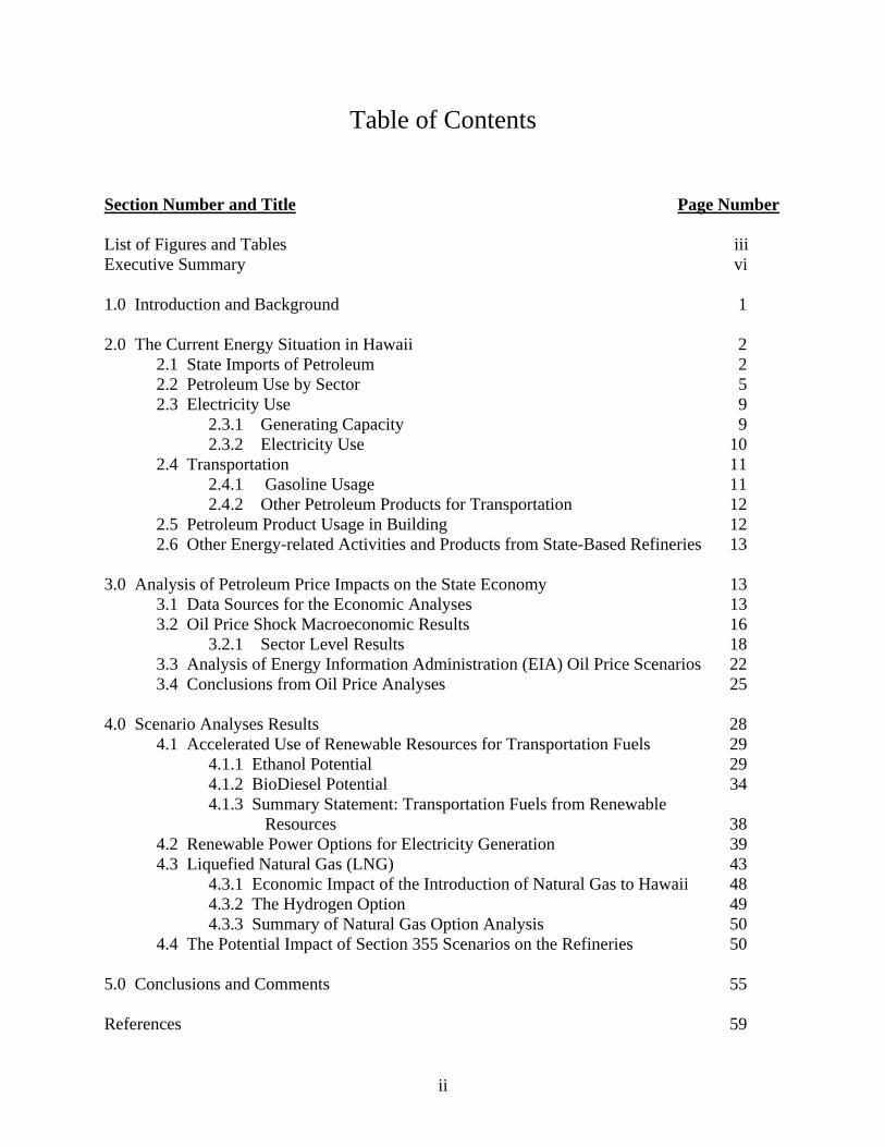
Table of Contents Section Number and Title Page Number List of Figures and Tables iii Executive Summary vi 1.0 Introduction and Background 1 2.0 The Current Energy Situation in Hawaii 2

2.1 State Imports of Petroleum 2 2.2 Petroleum Use by Sector 5 2.3 Electricity Use 9

2.3.1 Generating Capacity 9 2.3.2 Electricity Use 10

2.4 Transportation 11 2.4.1 Gasoline Usage 11 2.4.2 Other Petroleum Products for Transportation 12

2.5 Petroleum Product Usage in Building 12 2.6 Other Energy-related Activities and Products from State-Based Refineries 13

3.0 Analysis of Petroleum Price Impacts on the State Economy 13 3.1 Data Sources for the Economic Analyses 13 3.2 Oil Price Shock Macroeconomic Results 16

3.2.1 Sector Level Results 18 3.3 Analysis of Energy Information Administration (EIA) Oil Price Scenarios 22 3.4 Conclusions from Oil Price Analyses 25

4.0 Scenario Analyses Results 28

4.1 Accelerated Use of Renewable Resources for Transportation Fuels 29 4.1.1 Ethanol Potential 29 4.1.2 BioDiesel Potential 34 4.1.3 Summary Statement: Transportation Fuels from Renewable

Resources 38 4.2 Renewable Power Options for Electricity Generation 39 4.3 Liquefied Natural Gas (LNG) 43 4.3.1 Economic Impact of the Introduction of Natural Gas to Hawaii 48 4.3.2 The Hydrogen Option 49 4.3.3 Summary of Natural Gas Option Analysis 50 4.4 The Potential Impact of Section 355 Scenarios on the Refineries 50 5.0 Conclusions and Comments 55 References 59

ii

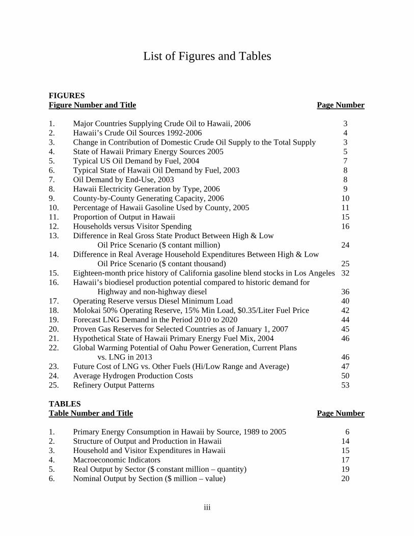
List of Figures and Tables FIGURES Figure Number and Title Page Number 1. Major Countries Supplying Crude Oil to Hawaii, 2006 3 2. Hawaii’s Crude Oil Sources 1992-2006 4 3. Change in Contribution of Domestic Crude Oil Supply to the Total Supply 3 4. State of Hawaii Primary Energy Sources 2005 5 5. Typical US Oil Demand by Fuel, 2004 7 6. Typical State of Hawaii Oil Demand by Fuel, 2003 8 7. Oil Demand by End-Use, 2003 8 8. Hawaii Electricity Generation by Type, 2006 9 9. County-by-County Generating Capacity, 2006 10 10. Percentage of Hawaii Gasoline Used by County, 2005 11 11. Proportion of Output in Hawaii 15 12. Households versus Visitor Spending 16 13. Difference in Real Gross State Product Between High & Low Oil Price Scenario ($ contant million) 24 14. Difference in Real Average Household Expenditures Between High & Low Oil Price Scenario ($ contant thousand) 25 15. Eighteen-month price history of California gasoline blend stocks in Los Angeles 32 16. Hawaii’s biodiesel production potential compared to historic demand for Highway and non-highway diesel 36 17. Operating Reserve versus Diesel Minimum Load 40 18. Molokai 50% Operating Reserve, 15% Min Load, $0.35/Liter Fuel Price 42 19. Forecast LNG Demand in the Period 2010 to 2020 44 20. Proven Gas Reserves for Selected Countries as of January 1, 2007 45 21. Hypothetical State of Hawaii Primary Energy Fuel Mix, 2004 46 22. Global Warming Potential of Oahu Power Generation, Current Plans vs. LNG in 2013 46 23. Future Cost of LNG vs. Other Fuels (Hi/Low Range and Average) 47 24. Average Hydrogen Production Costs 50 25. Refinery Output Patterns 53 TABLES Table Number and Title Page Number 1. Primary Energy Consumption in Hawaii by Source, 1989 to 2005 6 2. Structure of Output and Production in Hawaii 14 3. Household and Visitor Expenditures in Hawaii 15 4. Macroeconomic Indicators 17 5. Real Output by Sector ($ constant million – quantity) 19 6. Nominal Output by Section ($ million – value) 20

iii

List of Figures and Tables (continued)

TABLES (continued) Table Number and Title Page Number 7. Real Labor Payments by Sector ($ constant million) 20 8. Real Household Demand by Sector ($ constant million) 21 9. Real Visitor Demand by Sector ($ constant million) 22 10. Projected Population and Visitor Growth (1997 = 1) 22 11. EIA Crude Oil Price Projections ($/bbl) 23 12. Nominal Gross State Product ($ current billion) 23 13. Real Gross State Product ($ constant billion) 23 14. Real Average Household Expenditures ($ constant thousands) 24 15. Potential irrigated (<78”) and unirrigated (>78”) acreages zoned NRCS sugar soils by land designation 29 16. Ethanol potential from fermentable sugars from sugar cane grown on irrigated

and unirrigated acreages of agriculturally zoned NRCS sugar soils by land designation 29

17. Ethanol potential from sugar cane grown on irrigated and unirrigated acreages of agriculturally zoned NRCS sugar soils by land designation 30

18. Ethanol potential from sugar cane grown on irrigated agriculturally zoned NRCS sugar soils by land designation compared with actual usage 30

19. Summary table of statewide ethanol potential for four land groupings and four crop scenarios 34 20. Hawaiian Refinery Capacities (kb/d) 52 21. Typical Recent Oil Balances in Hawaii (kg/d) 53

iv

This page was left intentionally blank.

v

Executive Summary Introduction Hawaii is the most isolated island archipelago in the world. This isolation gives rise to certain challenges with respect to energy supply and security. For example, Hawaii relied on fossil fuels for nearly 95% of its energy needs as of 2006. Having no fossil fuel resources of its own, Hawaii must import all of its fossil fuel from abroad. This heavy reliance on imported energy puts the state in a vulnerable position with respect to energy security. The State of Hawaii Congressional delegation requested that Secretary of Energy Bodman fund a study which would examine the impacts on the state’s economy that would arise from the possible implementation of the three scenarios specified within Section 355 of Energy Policy Act of 2005. The first two scenarios are based on an evaluation of accelerated use of renewable resources for a) transportation fuels, and b) electricity generation. The third scenario required an evaluation of liquefied natural gas (LNG) being added to the energy resource mix in Hawaii. Given the basic shortcoming in the study scope and design highlighted in the original Scope of Work, the conclusions of the report have been written in three parts. The first part is one in which the analysis and data contained therein were sufficiently robust to warrant rather firm conclusions. The second area is one in which some conclusions can be made, with additional commentary on the need for future technical evaluation and analysis. The third area outlines those topics that are important to the study, but for which no conclusions can be made due to the lack of data or inability to obtain information for the analyses. This report is an integration of the other reports developed as part of the overall program. These reports are:

1. Current State of Hawaii’s Energy Resources and Utilization by Terry Surles and Milton Staackmann

2. Analysis of the Impact of Petroleum Prices on the State of Hawaii's Economy, by Makena Coffman, Terrence Surles, Denise Konan

3. Relationship of Refinery Operations and Oil-Fired Generation, by Terry Surles (based on material developed by FACTS in report #5)

4. Renewable Power Options for Electricity Generation: Molokai Case Study Leading to State-wide Analysis, by Peter Lilienthal, Alice Kandt, Blair Swezey (National Renewable Energy Laboratory – NREL), and Terry Surles (Hawaii Natural Energy Institute – HNEI)

5. Evaluating Natural Gas Options for the State of Hawaii, FACTS, Inc. 6. A Scenario for Accelerated Use of Renewable Resources for Transportation Fuels in

Hawaii, by Michael Foley, Scott Turn, Milton Staackmann, and Terry Surles

Numerous findings and observations are provided in these reports. Additionally, the methodology utilized to obtain and assess information and to perform the analyses is also discussed in greater detail in these reports.

vi

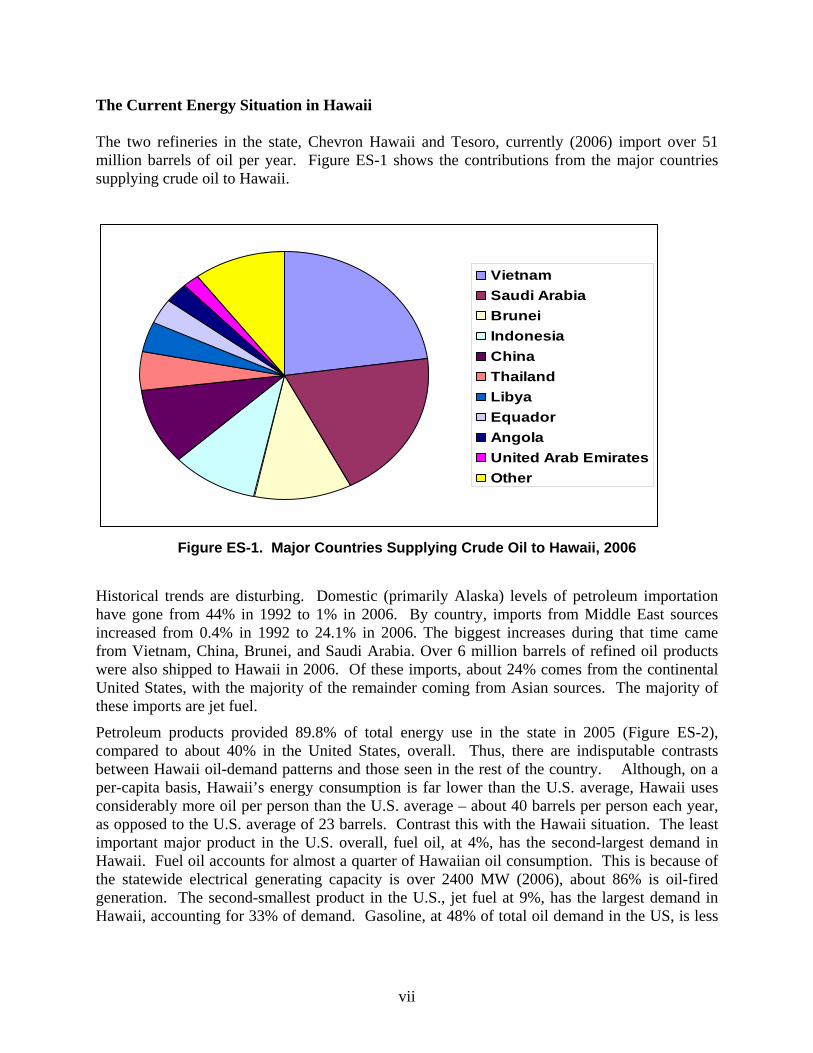
The Current Energy Situation in Hawaii The two refineries in the state, Chevron Hawaii and Tesoro, currently (2006) import over 51 million barrels of oil per year. Figure ES-1 shows the contributions from the major countries supplying crude oil to Hawaii.

VietnamSaudi ArabiaBruneiIndonesiaChinaThailandLibyaEquadorAngolaUnited Arab EmiratesOther

Figure ES-1. Major Countries Supplying Crude Oil to Hawaii, 2006

Historical trends are disturbing. Domestic (primarily Alaska) levels of petroleum importation have gone from 44% in 1992 to 1% in 2006. By country, imports from Middle East sources increased from 0.4% in 1992 to 24.1% in 2006. The biggest increases during that time came from Vietnam, China, Brunei, and Saudi Arabia. Over 6 million barrels of refined oil products were also shipped to Hawaii in 2006. Of these imports, about 24% comes from the continental United States, with the majority of the remainder coming from Asian sources. The majority of these imports are jet fuel.

Petroleum products provided 89.8% of total energy use in the state in 2005 (Figure ES-2), compared to about 40% in the United States, overall. Thus, there are indisputable contrasts between Hawaii oil-demand patterns and those seen in the rest of the country. Although, on a per-capita basis, Hawaii’s energy consumption is far lower than the U.S. average, Hawaii uses considerably more oil per person than the U.S. average – about 40 barrels per person each year, as opposed to the U.S. average of 23 barrels. Contrast this with the Hawaii situation. The least important major product in the U.S. overall, fuel oil, at 4%, has the second-largest demand in Hawaii. Fuel oil accounts for almost a quarter of Hawaiian oil consumption. This is because of the statewide electrical generating capacity is over 2400 MW (2006), about 86% is oil-fired generation. The second-smallest product in the U.S., jet fuel at 9%, has the largest demand in Hawaii, accounting for 33% of demand. Gasoline, at 48% of total oil demand in the US, is less

vii

than half as important in the Hawaiian demand barrel, making up only 20% of Hawaii’s oil demand.

Source: State of Hawaii Strategic Industries Division

Petroleum, 89.81%

Coal, 4.80%

Biomass, 1.63%

Municipal Solid Waste, 1.29%

Solar Hot Water, 1.38%

Photovoltaic, 0.01%

Hydroelectric, 0.35%

Geothermal, 0.70%

Wind, 0.02%

Figure ES-2. State of Hawaii Primary Energy Sources 2005

Results of Analyses Prior to examining the three scenario impacts, two oil price scenarios were examined. One was to evaluate the high oil price case from the Energy Information Administration. The second set of examples evaluated the impact of oil price volatility on the economy.

For the various oil price shock scenarios, a number of conclusions were reached. Sudden oil price shocks decrease real productivity, decrease real wages across sectors, and are inflationary overall. In the 100% increase scenario – a doubling of world oil prices – real gross state product declines by 3.7%, real wages decline by 1.3%, and the Hawaii consumer price index rises by 1.3%. While oil price shocks lead to inflationary pressure within an economy, both consumer demand shifts and the reduction in real visitor spending mean that oil price increases are also associated with deflationary effects. The inflationary effect nonetheless dominates throughout all examined shock levels.

Oil price increases mean a direct reduction in real petroleum manufacturing output (a decline of 34% in the 100% scenario), despite an increase in nominal petroleum manufacturing output. Increased oil prices impact the electricity sector through purchases from the state-based refineries. Electricity output declines in real terms (a decline of 13% in the 100% scenario). Air transportation declines by 9% in real terms in the 100% scenario, which has an implicit impact on the tourism industry in the state. The conclusions from the volatility analysis show how oil price volatility has large real economic impacts. In the short-run, even a 10% increase in world

viii

oil prices can have negative economic impacts, for instance a 0.5% decrease in real gross state product and a 0.16% increase in inflation.

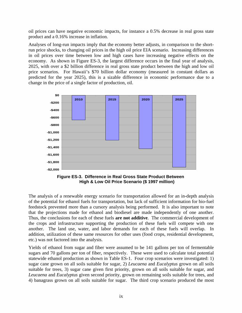
Analyses of long-run impacts imply that the economy better adjusts, in comparison to the short-run price shocks, to changing oil prices in the high oil price EIA scenario. Increasing differences in oil prices over time between low and high cases have increasing negative effects on the economy. As shown in Figure ES-3, the largest difference occurs in the final year of analysis, 2025, with over a $2 billion difference in real gross state product between the high and low oil price scenarios. For Hawaii’s $70 billion dollar economy (measured in constant dollars as predicted for the year 2025), this is a sizable difference in economic performance due to a change in the price of a single factor of production, oil.

-$2,000

-$1,800

-$1,600

-$1,400

-$1,200

-$1,000

-$800

-$600

-$400

-$200

$02010 2015 2020 2025

Figure ES-3. Difference in Real Gross State Product Between

High & Low Oil Price Scenario ($ 1997 million)

The analysis of a renewable energy scenario for transportation allowed for an in-depth analysis of the potential for ethanol fuels for transportation, but lack of sufficient information for bio-fuel feedstock prevented more than a cursory analysis being performed. It is also important to note that the projections made for ethanol and biodiesel are made independently of one another. Thus, the conclusions for each of these fuels are not additive. The commercial development of the crops and infrastructure supporting the production of these fuels will compete with one another. The land use, water, and labor demands for each of these fuels will overlap. In addition, utilization of these same resources for other uses (food crops, residential development, etc.) was not factored into the analysis.

Yields of ethanol from sugar and fiber were assumed to be 141 gallons per ton of fermentable sugars and 70 gallons per ton of fiber, respectively. These were used to calculate total potential statewide ethanol production as shown in Table ES-1. Four crop scenarios were investigated: 1) sugar cane grown on all soils suitable for sugar, 2) Leucaena and Eucalyptus grown on all soils suitable for trees, 3) sugar cane given first priority, grown on all soils suitable for sugar, and Leucaena and Eucalyptus given second priority, grown on remaining soils suitable for trees, and 4) banagrass grown on all soils suitable for sugar. The third crop scenario produced the most

ix

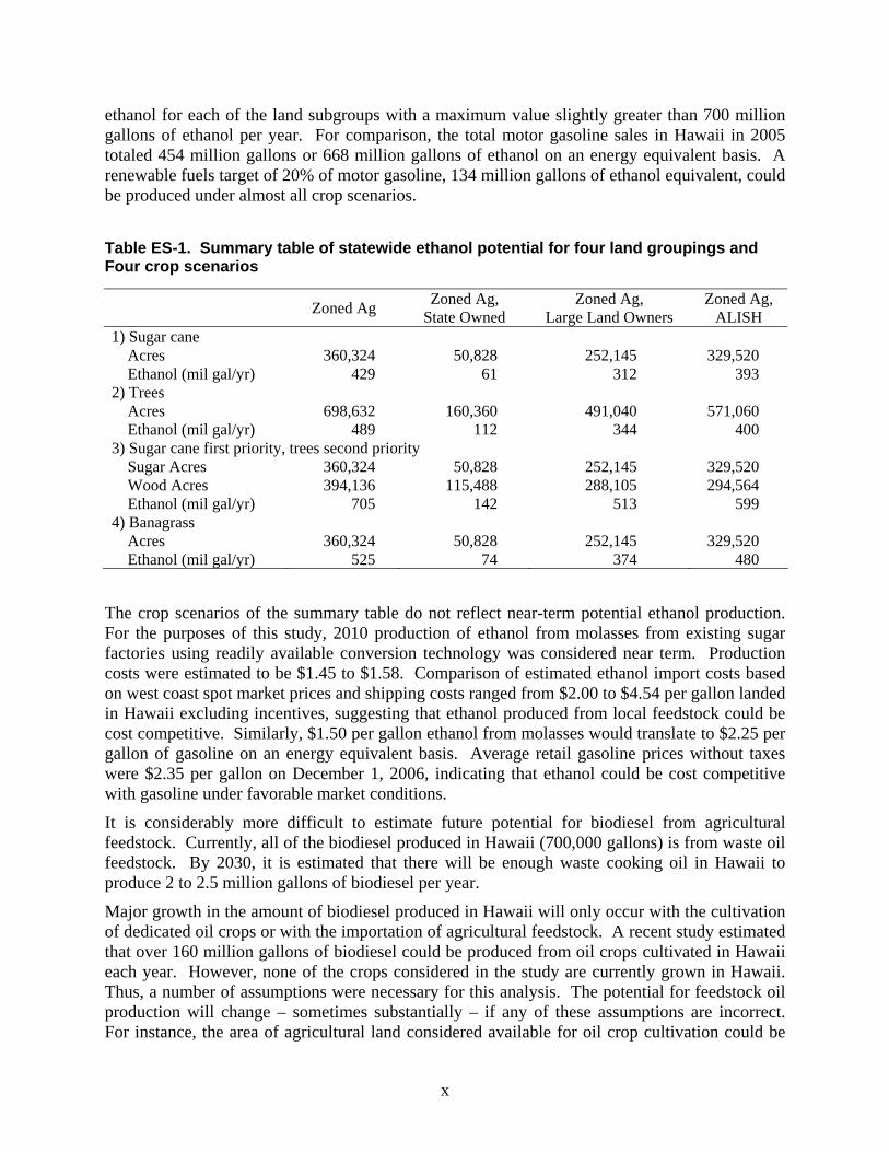
ethanol for each of the land subgroups with a maximum value slightly greater than 700 million gallons of ethanol per year. For comparison, the total motor gasoline sales in Hawaii in 2005 totaled 454 million gallons or 668 million gallons of ethanol on an energy equivalent basis. A renewable fuels target of 20% of motor gasoline, 134 million gallons of ethanol equivalent, could be produced under almost all crop scenarios. Table ES-1. Summary table of statewide ethanol potential for four land groupings and Four crop scenarios

Zoned Ag Zoned Ag, State Owned

Zoned Ag, Large Land Owners

Zoned Ag, ALISH

1) Sugar cane Acres 360,324 50,828 252,145 329,520 Ethanol (mil gal/yr) 429 61 312 393 2) Trees Acres 698,632 160,360 491,040 571,060 Ethanol (mil gal/yr) 489 112 344 400 3) Sugar cane first priority, trees second priority Sugar Acres 360,324 50,828 252,145 329,520 Wood Acres 394,136 115,488 288,105 294,564 Ethanol (mil gal/yr) 705 142 513 599 4) Banagrass Acres 360,324 50,828 252,145 329,520 Ethanol (mil gal/yr) 525 74 374 480

The crop scenarios of the summary table do not reflect near-term potential ethanol production. For the purposes of this study, 2010 production of ethanol from molasses from existing sugar factories using readily available conversion technology was considered near term. Production costs were estimated to be $1.45 to $1.58. Comparison of estimated ethanol import costs based on west coast spot market prices and shipping costs ranged from $2.00 to $4.54 per gallon landed in Hawaii excluding incentives, suggesting that ethanol produced from local feedstock could be cost competitive. Similarly, $1.50 per gallon ethanol from molasses would translate to $2.25 per gallon of gasoline on an energy equivalent basis. Average retail gasoline prices without taxes were $2.35 per gallon on December 1, 2006, indicating that ethanol could be cost competitive with gasoline under favorable market conditions.

It is considerably more difficult to estimate future potential for biodiesel from agricultural feedstock. Currently, all of the biodiesel produced in Hawaii (700,000 gallons) is from waste oil feedstock. By 2030, it is estimated that there will be enough waste cooking oil in Hawaii to produce 2 to 2.5 million gallons of biodiesel per year.

Major growth in the amount of biodiesel produced in Hawaii will only occur with the cultivation of dedicated oil crops or with the importation of agricultural feedstock. A recent study estimated that over 160 million gallons of biodiesel could be produced from oil crops cultivated in Hawaii each year. However, none of the crops considered in the study are currently grown in Hawaii. Thus, a number of assumptions were necessary for this analysis. The potential for feedstock oil production will change – sometimes substantially – if any of these assumptions are incorrect. For instance, the area of agricultural land considered available for oil crop cultivation could be

x

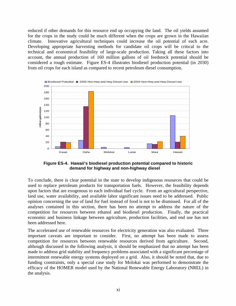
reduced if other demands for this resource end up occupying the land. The oil yields assumed for the crops in the study could be much different when the crops are grown in the Hawaiian climate. Innovative agricultural techniques could increase the oil potential of each acre. Developing appropriate harvesting methods for candidate oil crops will be critical to the technical and economical feasibility of large-scale production. Taking all these factors into account, the annual production of 160 million gallons of oil feedstock potential should be considered a rough estimate. Figure ES-4 illustrates biodiesel production potential (in 2030) from oil crops for each island as compared to recent petroleum diesel consumption.

0

20

40

60

80

100

120

140

160

180

200

Kauai Oahu Molokai Lanai Maui Hawaii

mill

ion

gallo

ns/y

ea

Biodiesel Potential 2005 Non-Hwy and Hwy Diesel Use 2004 Non-Hwy and Hwy Diesel Use

Figure ES-4. Hawaii’s biodiesel production potential compared to historic

demand for highway and non-highway diesel To conclude, there is clear potential in the state to develop indigenous resources that could be used to replace petroleum products for transportation fuels. However, the feasibility depends upon factors that are exogenous to each individual fuel cycle. From an agricultural perspective, land use, water availability, and available labor significant issues need to be addressed. Public opinion concerning the use of land for fuel instead of food is not to be dismissed. For all of the analyses contained in this section, there has been no attempt to address the nature of the competition for resources between ethanol and biodiesel production. Finally, the practical economic and business linkage between agriculture, production facilities, and end use has not been addressed here.

The accelerated use of renewable resources for electricity generation was also evaluated. Three important caveats are important to consider. First, no attempt has been made to assess competition for resources between renewable resources derived from agriculture. Second, although discussed in the following analysis, it should be emphasized that no attempt has been made to address grid stability and frequency problems associated with a significant percentage of intermittent renewable energy systems deployed on a grid. Also, it should be noted that, due to funding constraints, only a special case study for Molokai was performed to demonstrate the efficacy of the HOMER model used by the National Renewable Energy Laboratory (NREL) in the analysis.

xi

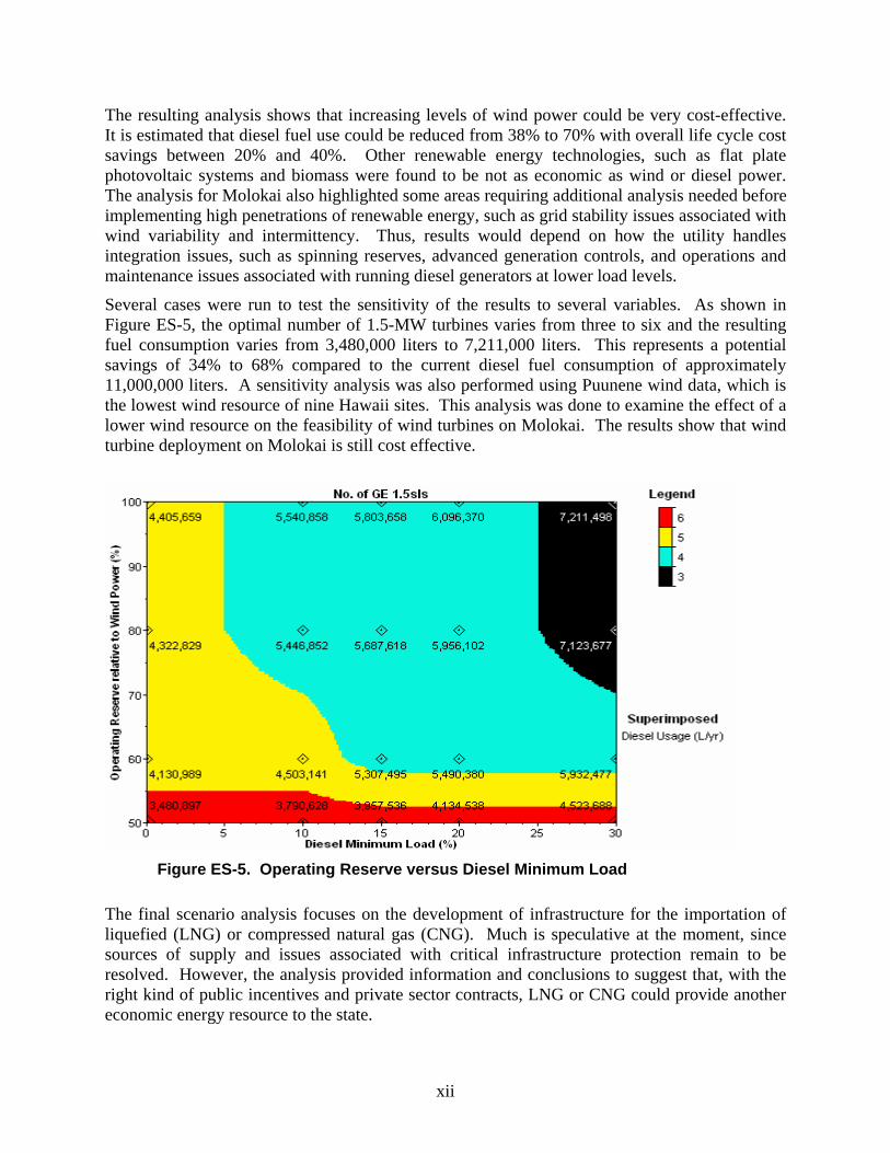
The resulting analysis shows that increasing levels of wind power could be very cost-effective. It is estimated that diesel fuel use could be reduced from 38% to 70% with overall life cycle cost savings between 20% and 40%. Other renewable energy technologies, such as flat plate photovoltaic systems and biomass were found to be not as economic as wind or diesel power. The analysis for Molokai also highlighted some areas requiring additional analysis needed before implementing high penetrations of renewable energy, such as grid stability issues associated with wind variability and intermittency. Thus, results would depend on how the utility handles integration issues, such as spinning reserves, advanced generation controls, and operations and maintenance issues associated with running diesel generators at lower load levels.

Several cases were run to test the sensitivity of the results to several variables. As shown in Figure ES-5, the optimal number of 1.5-MW turbines varies from three to six and the resulting fuel consumption varies from 3,480,000 liters to 7,211,000 liters. This represents a potential savings of 34% to 68% compared to the current diesel fuel consumption of approximately 11,000,000 liters. A sensitivity analysis was also performed using Puunene wind data, which is the lowest wind resource of nine Hawaii sites. This analysis was done to examine the effect of a lower wind resource on the feasibility of wind turbines on Molokai. The results show that wind turbine deployment on Molokai is still cost effective.

Figure ES-5. Operating Reserve versus Diesel Minimum Load

The final scenario analysis focuses on the development of infrastructure for the importation of liquefied (LNG) or compressed natural gas (CNG). Much is speculative at the moment, since sources of supply and issues associated with critical infrastructure protection remain to be resolved. However, the analysis provided information and conclusions to suggest that, with the right kind of public incentives and private sector contracts, LNG or CNG could provide another economic energy resource to the state.

xii

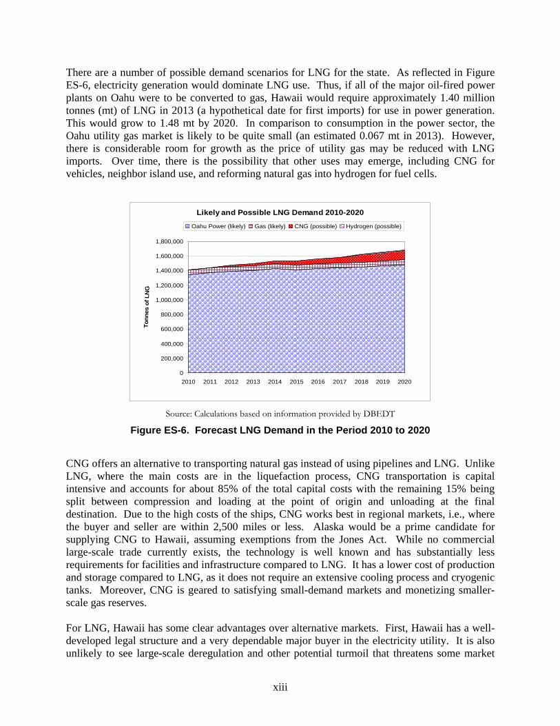
There are a number of possible demand scenarios for LNG for the state. As reflected in Figure ES-6, electricity generation would dominate LNG use. Thus, if all of the major oil-fired power plants on Oahu were to be converted to gas, Hawaii would require approximately 1.40 million tonnes (mt) of LNG in 2013 (a hypothetical date for first imports) for use in power generation. This would grow to 1.48 mt by 2020. In comparison to consumption in the power sector, the Oahu utility gas market is likely to be quite small (an estimated 0.067 mt in 2013). However, there is considerable room for growth as the price of utility gas may be reduced with LNG imports. Over time, there is the possibility that other uses may emerge, including CNG for vehicles, neighbor island use, and reforming natural gas into hydrogen for fuel cells.

Likely and Possible LNG Demand 2010-2020

0

200,000

400,000

600,000

800,000

1,000,000

1,200,000

1,400,000

1,600,000

1,800,000

2010 2011 2012 2013 2014 2015 2016 2017 2018 2019 2020

Tonn

es o

f LN

G

Oahu Power (likely) Gas (likely) CNG (possible) Hydrogen (possible)

Source: Calculations based on information provided by DBEDT

Figure ES-6. Forecast LNG Demand in the Period 2010 to 2020

CNG offers an alternative to transporting natural gas instead of using pipelines and LNG. Unlike LNG, where the main costs are in the liquefaction process, CNG transportation is capital intensive and accounts for about 85% of the total capital costs with the remaining 15% being split between compression and loading at the point of origin and unloading at the final destination. Due to the high costs of the ships, CNG works best in regional markets, i.e., where the buyer and seller are within 2,500 miles or less. Alaska would be a prime candidate for supplying CNG to Hawaii, assuming exemptions from the Jones Act. While no commercial large-scale trade currently exists, the technology is well known and has substantially less requirements for facilities and infrastructure compared to LNG. It has a lower cost of production and storage compared to LNG, as it does not require an extensive cooling process and cryogenic tanks. Moreover, CNG is geared to satisfying small-demand markets and monetizing smaller-scale gas reserves. For LNG, Hawaii has some clear advantages over alternative markets. First, Hawaii has a well-developed legal structure and a very dependable major buyer in the electricity utility. It is also unlikely to see large-scale deregulation and other potential turmoil that threatens some market

xiii

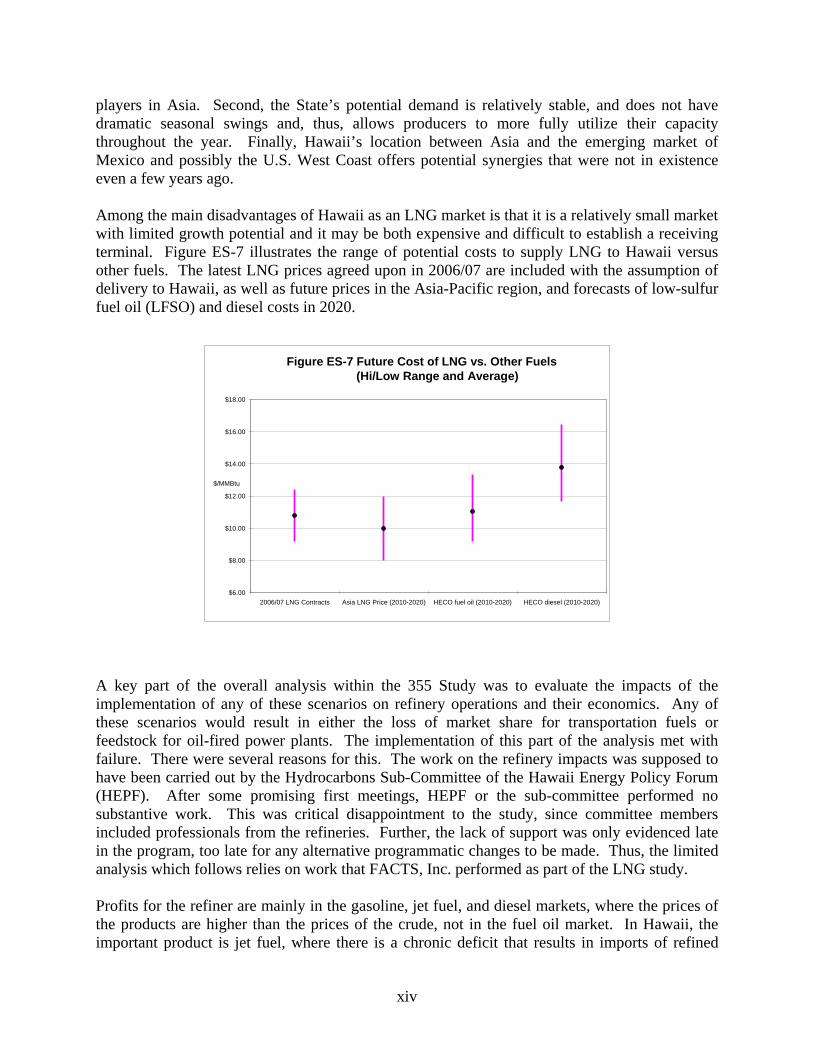
players in Asia. Second, the State’s potential demand is relatively stable, and does not have dramatic seasonal swings and, thus, allows producers to more fully utilize their capacity throughout the year. Finally, Hawaii’s location between Asia and the emerging market of Mexico and possibly the U.S. West Coast offers potential synergies that were not in existence even a few years ago. Among the main disadvantages of Hawaii as an LNG market is that it is a relatively small market with limited growth potential and it may be both expensive and difficult to establish a receiving terminal. Figure ES-7 illustrates the range of potential costs to supply LNG to Hawaii versus other fuels. The latest LNG prices agreed upon in 2006/07 are included with the assumption of delivery to Hawaii, as well as future prices in the Asia-Pacific region, and forecasts of low-sulfur fuel oil (LFSO) and diesel costs in 2020.

Figure ES-7 Future Cost of LNG vs. Other Fuels (Hi/Low Range and Average)

$6.00

$8.00

$10.00

$12.00

$14.00

$16.00

$18.00

2006/07 LNG Contracts Asia LNG Price (2010-2020) HECO fuel oil (2010-2020) HECO diesel (2010-2020)

$/MMBtu

A key part of the overall analysis within the 355 Study was to evaluate the impacts of the implementation of any of these scenarios on refinery operations and their economics. Any of these scenarios would result in either the loss of market share for transportation fuels or feedstock for oil-fired power plants. The implementation of this part of the analysis met with failure. There were several reasons for this. The work on the refinery impacts was supposed to have been carried out by the Hydrocarbons Sub-Committee of the Hawaii Energy Policy Forum (HEPF). After some promising first meetings, HEPF or the sub-committee performed no substantive work. This was critical disappointment to the study, since committee members included professionals from the refineries. Further, the lack of support was only evidenced late in the program, too late for any alternative programmatic changes to be made. Thus, the limited analysis which follows relies on work that FACTS, Inc. performed as part of the LNG study. Profits for the refiner are mainly in the gasoline, jet fuel, and diesel markets, where the prices of the products are higher than the prices of the crude, not in the fuel oil market. In Hawaii, the important product is jet fuel, where there is a chronic deficit that results in imports of refined

xiv

product from as far away as the Middle East. The two Hawaiian refineries are both relatively small facilities by current world standards; today, world-scale refineries are typically 125-250 thousand barrels per day (kb/d) in size. The Chevron refinery, the older of the two, is about 54 kb/d. The newer Tesoro refinery is about 93 kb/d. The refineries are both equipped with cracking facilities and other units to assist in upgrading the output slate into more valuable products. The Chevron refinery is equipped with catalytic cracking, a technology that breaks part of the fuel oil into gasoline (and also creates ‘cycle oils,’ which are blended back into the remaining fuel oil to lower the viscosity). Chevron also has alkylation and isomerization units, which take some of the gases from processing and turn them into high-octane blendstocks for gasoline.

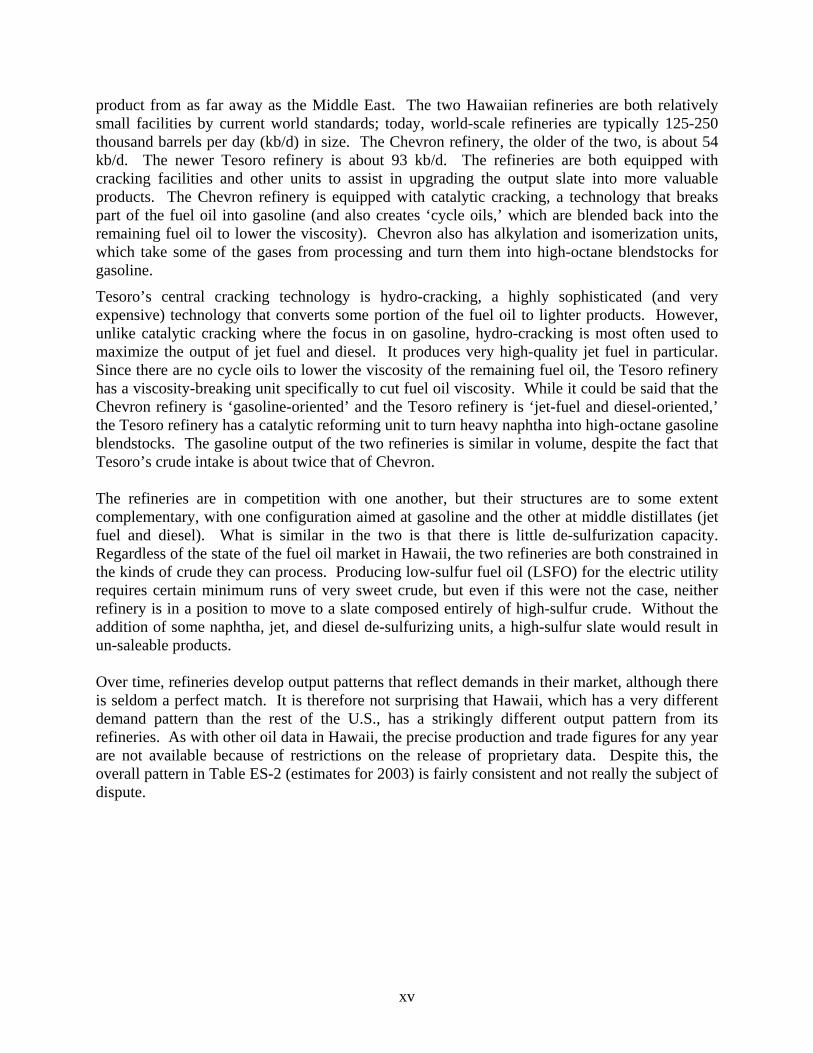
Tesoro’s central cracking technology is hydro-cracking, a highly sophisticated (and very expensive) technology that converts some portion of the fuel oil to lighter products. However, unlike catalytic cracking where the focus in on gasoline, hydro-cracking is most often used to maximize the output of jet fuel and diesel. It produces very high-quality jet fuel in particular. Since there are no cycle oils to lower the viscosity of the remaining fuel oil, the Tesoro refinery has a viscosity-breaking unit specifically to cut fuel oil viscosity. While it could be said that the Chevron refinery is ‘gasoline-oriented’ and the Tesoro refinery is ‘jet-fuel and diesel-oriented,’ the Tesoro refinery has a catalytic reforming unit to turn heavy naphtha into high-octane gasoline blendstocks. The gasoline output of the two refineries is similar in volume, despite the fact that Tesoro’s crude intake is about twice that of Chevron. The refineries are in competition with one another, but their structures are to some extent complementary, with one configuration aimed at gasoline and the other at middle distillates (jet fuel and diesel). What is similar in the two is that there is little de-sulfurization capacity. Regardless of the state of the fuel oil market in Hawaii, the two refineries are both constrained in the kinds of crude they can process. Producing low-sulfur fuel oil (LSFO) for the electric utility requires certain minimum runs of very sweet crude, but even if this were not the case, neither refinery is in a position to move to a slate composed entirely of high-sulfur crude. Without the addition of some naphtha, jet, and diesel de-sulfurizing units, a high-sulfur slate would result in un-saleable products. Over time, refineries develop output patterns that reflect demands in their market, although there is seldom a perfect match. It is therefore not surprising that Hawaii, which has a very different demand pattern than the rest of the U.S., has a strikingly different output pattern from its refineries. As with other oil data in Hawaii, the precise production and trade figures for any year are not available because of restrictions on the release of proprietary data. Despite this, the overall pattern in Table ES-2 (estimates for 2003) is fairly consistent and not really the subject of dispute.

xv

Table ES-2 Typical Recent Oil Balances in Hawaii (kb/d)Demand Production Imports* Exports*

LPG 1. 6 1.6 Naphtha 6. 0 1 3.5 7 .5 Gasoline 29 .0 2 9.0 Jet Fuel 41 .0 3 2.5 8 .5 Diesel 26 .0 2 6.0 Fuel Oil 33 .0 3 0.5 2 .5 Other 1. 5 1.5

1 38.1 1 34.6 1 1.0 7 .5 *Imports and exports are on a net basis; there are smallmovements in and out for commercial reasons whichare not captured in this table

Compared to many supply/demand systems around the world, the Hawaiian refinery system is surprisingly well balanced (apart for the substantial jet fuel deficit). The system is also running fairly close to capacity. While economics might seem to favor production of more jet fuel, it is impossible to produce more jet fuel without also producing a small surplus of other products. If a Hawaii refinery were to shut down, there are a number of potential drawbacks that should be considered. First, consider energy security. If any of these scenarios leads to the closure of a refinery, the State would have to import larger quantities of refined petroleum products. The State would require a variety of products, which may not be as widely traded as crude oil. For the case of the refinery staying open, some immediate effects could include a change in the crude slate, a further shift to light crude, and a decline in overall crude runs to avoid large exports of fuel oil, such as in the case of the LNG scenario. Several outcomes for the refining industry are possible if portions of the petroleum products market are eliminated. The industry can retrench and adapt. New investments might be undertaken to allow the refiners more flexibility in the crude diet. Or, at the extreme, the industry might be consolidated, expanded, and upgraded to meet the needs of the export market in addition to remaining local demands. What needs to be stressed is that a number of outcomes are possible. Slashing the demand for LFSO or for gasoline will put new pressure on the refiners, but it is only one of many challenges they face. The closure of one or both refineries is neither inevitable nor does it necessarily lower the competitiveness of the market in Hawaii. Indeed, if steps are taken to ensure that a wider selection of fuel suppliers have access to the market (especially in terms of import infrastructure), then price competition might actually be strengthened. It should be noted, however, that this might not happen through purely market forces. The State might have to take a role in ensuring wider access to terminals and tankage. Conclusions and Comments While there are some very useful analyses contained in this report, it is seriously flawed. The primary reason for this serious flaw is that the key point – the economic impact to the state due to changes in oil resource requirements – was not examined. Specifically, there can no true analysis of the impact to the state’s economy based on any one of the three scenarios contained

xvi

in Section 355 without being able to examine the impact on refinery operations. Thus, any analysis, other than hypothesis and conjecture, would need to be based on a set of assumptions that have yet to be validated. Thus, a qualitative evaluation of the impact to the state’s economy is lacking and this is a serious drawback to the overall study. It should also be noted that the scenarios contained within Section 355 do not provide for an analysis of one of the more obvious approaches to reduction in petroleum dependency. All of the scenarios are supply-side scenarios and do not address opportunities with demand-side technologies. Specifically, such a scenario would focus on end-use energy efficiency and peak-demand reduction. Improvements in technologies in both cases would lead to a significant reduction in petroleum dependency. Any future analyses must necessarily examine end-use energy-efficiency scenarios. The following is the summary of conclusions sorted by the three categories highlighted in the Scope of Work. Category 1 products are intended to illustrate that sufficient work had been done to preclude a need for further analysis. The current state of the state, in terms of energy use and supply, has been examined. However, there is an on-going need to continue this work. This is because changes in state policy, technological advances, national policy, and geo-political supply and demand issues require a continual re-evaluation of the state’s energy situation. These analyses must support development of policies by government that ensure sound economic and environmental approaches for maintaining energy supplies as a result of price volatility and security issues. Category 2 products are those for which there are sufficient data to reach conclusions, but for which additional evaluation or data gathering is required to make the final results more robust. Although University of Hawaii Economic Research Organization (UHERO) models work reasonably well in forecasting future impacts associated with price volatility and increases, it is also clear, after exercising these modeling systems, that additional funding is needed to make them more robust for future analyses. The more robust nature of modeling systems can be an important attribute for supporting state policies and increasing the intellectual capacity and technical capabilities of institutions within the state. Per the study in which the UHERO models were utilized, analyses showed that both longer-term linear oil price increases and volatile oil prices have a significant impact on the state economy. Further, for industrial sectors, such as petroleum refining and electricity, that would stand to gain from high energy prices, it was shown that these gains in real dollar terms are illusory. It was also illustrated that volatility appeared to have a greater impact on the economy than slower, but steady, increases in oil prices.

For the renewable resources for transportation scenario, it was shown that under a certain set of assumptions, ethanol production in the state could provide most, if not all, of the transportation fuel needs for the state. However, these assumptions were made without regard to exogenous requirements, such as those for water, land, and labor. A similar conclusion cannot be reached for biodiesel fuel production. Feedstock to produce biodiesel for transportation fuels could be grown in the state. However, too little is known about the economics and the related agricultural requirements about any feedstock to make an accurate assessment as to the potential for future production.

xvii

xviii

For the liquefied natural gas (LNG) scenario, a rigorous analysis determined that there is the potential for LNG to displace low-sulfur fuel oil as the energy resource for fossil-fired power plants in the state and, in particular, on Oahu. The need for more analysis would center on the economic ability and societal interest to develop the necessary infrastructure to accept LNG, the surety of supplies from foreign sources, and the potential of using compressed natural gas due to smaller investment needs for infrastructure development.

For the renewable resources for electricity generation scenario, it was shown that the NREL models can be used to provide an analysis of renewable energy system penetration for displacement of fossil fuel for small-scale island systems, such as Molokai. This analysis demonstrated that wind turbines, even with a substantial amount of spinning reserve requirements, could displace substantial amounts of diesel power.

Category 3 products are those where sufficiently robust data are lacking for reasonable conclusions or recommendations. Due to the lack of information on refinery impacts, there was no substantive analytical work performed as part of this study on the effects of any of the scenarios on the operations, economics, and modified product mix associated with either of the state-based refineries. The lack of information prevents the completion of the final integrated analysis of impacts to the economy resulting from significant reduction of petroleum demand in the state. The results from this integrated assessment would provide public policy makers with a set of information that could be used to develop policies to reduce the state’s dependence on petroleum, while minimizing exogenous economic impacts that would result from changes in the energy resource mix. Recommendation Lacking sufficient key information, there is a clear need to continue these efforts. The lack of support from some groups on the original team notwithstanding, the overall effort allowed for the development of a strong project team that included two University of Hawaii organizations, the National Renewable Energy Laboratory, and FACTS Global Research. It is the bottom-line recommendation of the study that this work be continued to closure with the current study team. This team possesses the requisite skills, expertise, and analytical tools and models to bring the overall effort to a successful close. The result will be what was originally intended in the EPACT Section 355 legislation: specifically, to develop a set of recommendations to be used by public policy decision-makers for new approaches for reducing the dependence of the state on petroleum.

Integrated Summary Report: Evaluation of Economic Impacts Due to Changes in Petroleum Prices and Utilization 1.0 Introduction and Background

Hawaii is the most isolated island archipelago in the world. Its nearest continental neighbor is North America, nearly 2,400 miles away [1]. This isolation gives rise to certain challenges with respect to energy supply and security. Hawaii relied on fossil fuels for almost 95% of its energy needs as of 2005 [2]. Having no fossil fuel resources of its own, Hawaii must import all of its fossil fuel from abroad. This heavy reliance on imported energy puts the state in a vulnerable position with respect to energy security. Because of this fact, Section 355 of the Energy Policy Act of 2005 (EPACT) contains language which requires the examination of the impacts on the state that currently result from excessive dependence on fossil fuels and the potential impacts on the state’s economy which might result from a decreased dependence on these fuels.

The focus of the analysis within this effort is on energy security for the state of Hawaii, with the clear emphasis on addressing impacts related to decreased reliance of the state on petroleum products. In addition, while not explicit, there is clearly a relationship between these analyses and scenarios with addressing mechanisms for reducing global climate change impacts. All three scenarios, either by using renewable resources or by using liquefied natural gas address various forms of resource or fuel switching, resulting in fewer carbon dioxide emission per unit of energy produced.

While originally an authorization within EPACT, the State of Hawaii Congressional delegation requested that Secretary of Energy Bodman fund a study which would examine the impacts on the state’s economy that would arise from the possible implementation of the three scenarios specified within Section 355 of EPACT [3,4].

The first two scenarios were based on an evaluation of accelerated use of renewable resources for a) transportation fuels, and b) electricity generation. The third scenario required an evaluation of incorporation of liquefied natural gas (LNG) into the energy resource mix in Hawaii. The analyses performed as part of this study examined each of these resource scenarios separately. That is, there was no attempt to evaluate possible interactions and trade-offs between these scenarios.

Given the basic shortcoming in the study scope and design, the Scope of Work was written explicitly to address what might be anticipated as shortcomings in the report. Therefore, the conclusions of the report have been written in a way that outlines three sets of conclusions. The first set is one in which the analysis and data contained therein were sufficiently robust to warrant rather firm conclusions. The second area is one in which some conclusions can be made, with additional commentary on the need for future technical evaluation and analysis. The third area outlines those topics which are

1

important to the study, but for which no conclusions can be made due to the lack of data or inability to obtain information for the analyses.

In order to develop the best set of data and to conduct appropriate analyses for these scenarios, a team was assembled in 2006 to address these issues. Many of these organizations then led the development of the documentation for the analyses that form the basis for this integrating report. These organizations included:

- University of Hawaii, Hawaii Natural Energy Institute (HNEI), - University of Hawaii, Economic Research Organization (UHERO), - National Renewable Energy Laboratory (NREL), - FACTS Global Research, as supported by funding from this program and

from the Office of Hawaiian Affairs (OHA), and - Hawaii Energy Policy Forum (HEPF).

HNEI was in charge of the overall study. The contributions of the individual organizations will be highlighted in the following chapters. The chapters are arranged as follows. Chapter 2 provides a brief overview of the state energy situation with an emphasis on oil. Chapter 3 examines economic impacts to the state based on the volatility of oil prices and the longer-term trends towards increasing prices for petroleum. Chapter 4 provides a summary of the analyses performed that examine the impacts to the state associated with implementation of the scenarios described previously. Chapter 5 will offer some conclusions, observations, and recommendations that have resulted from this effort. 2.0 The Current Energy Situation in Hawaii The following discussion focuses on the importation and utilization of petroleum by the refineries and by the state. While it is important to understand that other resources are available to the state (e.g., coal, solar, geothermal, and energy efficient technologies), the nature of the Section 355 analysis requires a focus on petroleum use. Thus, this chapter offers an overview that stresses the current dependence on petroleum by the state.

2.1 State Imports of Petroleum

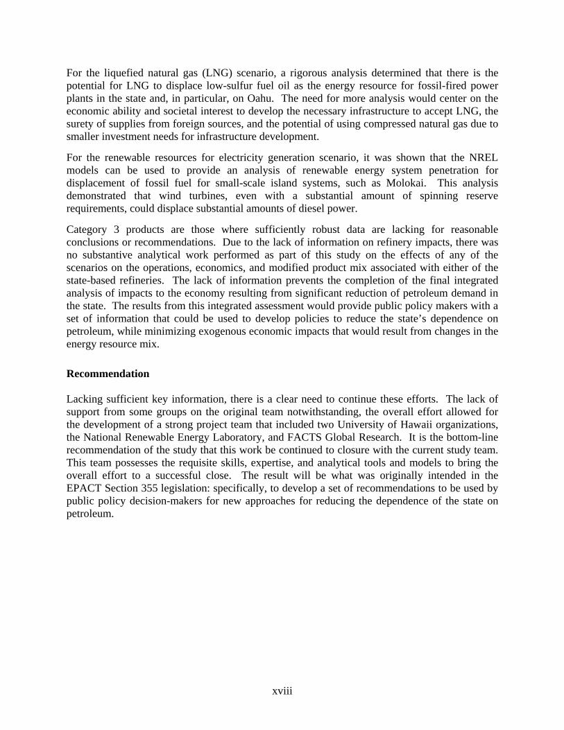
The two refineries in the state, Chevron Hawaii and Tesoro, currently (2006) import over 51 million barrels of oil per year (51,340,000 according to DBEDT). These supplies come from a number of countries. In order of descending amounts, the top ten suppliers in 2006 were Vietnam, Saudi Arabia, Brunei, Indonesia, China, Thailand, Libya, Ecuador, Angola, and United Arab Emirates. Figure 1 below shows the contributions from the major countries supplying crude oil to Hawaii.

2

Sources: State of Hawaii Strategic Industries Division, and U.S. Energy Information Agency - 2007: Preliminary - May 2007

VietnamSaudi ArabiaBruneiIndonesiaChinaThailandLibyaEquadorAngolaUnited Arab EmiratesOther

Figure 1 Major Countries Supplying Crude Oil to Hawaii, 2006

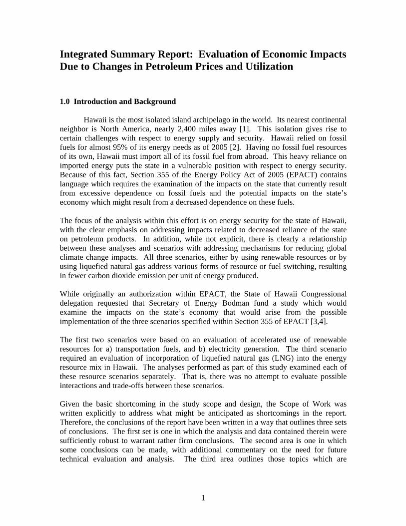
Figure 2 on the following page shows the history of crude oil sources for Hawaii, 1992-2006. Some trends are a bit disturbing. Domestic (primarily Alaska) levels of petroleum importation have gone from 44% in 1992 to less than 1% in 2006 (see Figure 3 below). By country, imports from Middle East sources increased from 0.4% in 1992 to 24.1% in 2006. The biggest increases during that time came from Vietnam, Saudi Arabia, Brunei, and China, with a significant percentage decrease from Indonesia. Note that recent increases in supplies from the Middle East are due to the new requirement for low sulfur oil. The state-based refineries are not set up to produce products from feedstock that contains a substantial amount of sulfur.

19922006

Domestic Supply

Foreign Suppliers

0.0%10.0%20.0%30.0%40.0%50.0%60.0%70.0%80.0%90.0%

100.0%

Sources: State of Hawaii Strategic Industries Division, and U.S. Energy Information Agency - 2007: Preliminary - May 2007

DomesticSupply

ForeignSuppliers

Figure 3 Change in Contribution of Domestic Crude Oil

Supply to the Total Supply

3

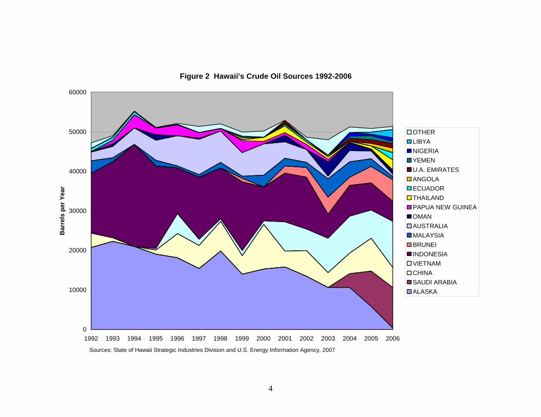
Figure 2 Hawaii's Crude Oil Sources 1992-2006

0

10000

20000

30000

40000

50000

60000

1992 1993 1994 1995 1996 1997 1998 1999 2000 2001 2002 2003 2004 2005 2006

Bar

rels

per

Yea

r

OTHERLIBYANIGERIAYEMENU.A. EMIRATESANGOLAECUADORTHAILANDPAPUA NEW GUINEAOMANAUSTRALIAMALAYSIABRUNEIINDONESIAVIETNAMCHINASAUDI ARABIAALASKA

Sources: State of Hawaii Strategic Industries Division and U.S. Energy Information Agency, 2007

4

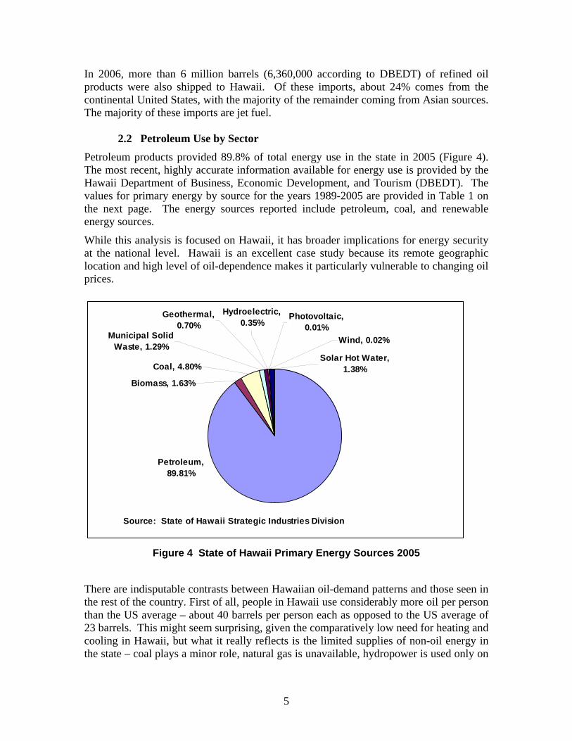
In 2006, more than 6 million barrels (6,360,000 according to DBEDT) of refined oil products were also shipped to Hawaii. Of these imports, about 24% comes from the continental United States, with the majority of the remainder coming from Asian sources. The majority of these imports are jet fuel. 2.2 Petroleum Use by Sector Petroleum products provided 89.8% of total energy use in the state in 2005 (Figure 4). The most recent, highly accurate information available for energy use is provided by the Hawaii Department of Business, Economic Development, and Tourism (DBEDT). The values for primary energy by source for the years 1989-2005 are provided in Table 1 on the next page. The energy sources reported include petroleum, coal, and renewable energy sources.

While this analysis is focused on Hawaii, it has broader implications for energy security at the national level. Hawaii is an excellent case study because its remote geographic location and high level of oil-dependence makes it particularly vulnerable to changing oil prices.

Source: State of Hawaii Strategic Industries Division

Petroleum, 89.81%

Coal, 4.80%

Biomass, 1.63%

Municipal Solid Waste, 1.29%

Solar Hot Water, 1.38%

Photovoltaic, 0.01%

Hydroelectric, 0.35%

Geothermal, 0.70%

Wind, 0.02%

Figure 4 State of Hawaii Primary Energy Sources 2005

There are indisputable contrasts between Hawaiian oil-demand patterns and those seen in the rest of the country. First of all, people in Hawaii use considerably more oil per person than the US average – about 40 barrels per person each as opposed to the US average of 23 barrels. This might seem surprising, given the comparatively low need for heating and cooling in Hawaii, but what it really reflects is the limited supplies of non-oil energy in the state – coal plays a minor role, natural gas is unavailable, hydropower is used only on

5

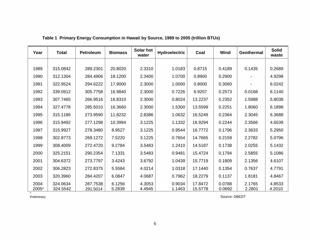
Table 1 Primary Energy Consumption in Hawaii by Source, 1989 to 2005 (trillion BTUs)

Year Total Petroleum Biomass Solar hot water Hydroelectric Coal Wind Geothermal Solid

waste

1989 315.0842 289.2301 20.8020 2.3310 1.0183 0.8715 0.4189 0.1435 0.2689

1990 312.1304 284.4906 18.1200 2.3400 1.0700 0.8900 0.2900 - 4.9298

1991 322.9524 294.6222 17.9000 2.3000 1.0000 0.8000 0.3060 - 6.0242

1992 339.0912 305.7758 16.9840 2.3000 0.7226 6.9207 0.2573 0.0168 6.1140

1993 307.7465 266.9516 16.8310 2.3000 0.8024 13.2237 0.2352 1.5988 5.8038

1994 327.4778 285.5010 16.3660 2.3000 1.5300 13.5599 0.2251 1.8060 6.1898

1995 315.1186 273.9590 11.8232 2.8386 1.0632 16.5249 0.2364 2.3045 6.3688

1996 315.9492 277.1298 10.3994 3.1225 1.1332 16.9294 0.2244 2.3566 4.6539

1997 315.9927 278.3480 8.9527 3.1225 0.9544 16.7772 0.1796 2.3633 5.2950

1998 302.8773 269.1272 7.5220 3.1225 0.7654 14.7665 0.2159 2.2782 5.0796

1999 308.4009 272.4720 9.2784 3.5483 1.2410 14.5187 0.1738 2.0255 5.1432

2000 325.2151 290.2354 7.1331 3.5483 0.9481 15.4724 0.1794 2.5855 5.1086

2001 304.6372 273.7797 3.4243 3.6792 1.0439 15.7719 0.1809 2.1356 4.6107

2002 306.2823 272.8375 5.5584 4.0214 1.0318 17.1440 0.1354 0.7637 4.7791

2003 320.3960 284.4207 6.0847 4.0687 0.7962 18.2279 0.1137 1.8181 4.8467

2004 324.0634 287.7538 6.1256 4.3053 0.9034 17.8472 0.0788 2.1765 4.8533 2005* 324.5542 291.5014 5.2839 4.4945 1.1463 15.5778 0.0692 2.2801 4.2010

* Preliminary Source: DBEDT

6

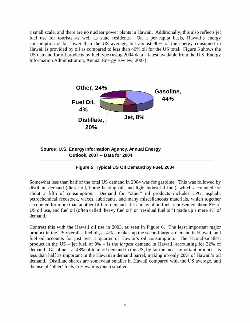
a small scale, and there are no nuclear power plants in Hawaii. Additionally, this also reflects jet fuel use for tourists as well as state residents. On a per-capita basis, Hawaii’s energy consumption is far lower than the US average, but almost 90% of the energy consumed in Hawaii is provided by oil as compared to less than 40% oil for the US total. Figure 5 shows the US demand for oil products by fuel type (using 2004 data – latest available from the U.S. Energy Information Administration, Annual Energy Review, 2007).

Source: U.S. Energy Information Agency, Annual Energy Outlook, 2007 -- Data for 2004

Gasoline, 44%

Jet, 8%Distillate, 20%

Fuel Oil, 4%

Other, 24%

Figure 5 Typical US Oil Demand by Fuel, 2004

Somewhat less than half of the total US demand in 2004 was for gasoline. This was followed by distillate demand (diesel oil, home heating oil, and light industrial fuel), which accounted for about a fifth of consumption. Demand for “other” oil products includes LPG, asphalt, petrochemical feedstock, waxes, lubricants, and many miscellaneous materials, which together accounted for more than another fifth of demand. Jet and aviation fuels represented about 8% of US oil use, and fuel oil (often called ‘heavy fuel oil’ or ‘residual fuel oil’) made up a mere 4% of demand. Contrast this with the Hawaii oil use in 2003, as seen in Figure 6. The least important major product in the US overall – fuel oil, at 4% – makes up the second-largest demand in Hawaii, and fuel oil accounts for just over a quarter of Hawaii’s oil consumption. The second-smallest product in the US – jet fuel, at 9% – is the largest demand in Hawaii, accounting for 32% of demand. Gasoline – at 48% of total oil demand in the US, by far the most important product – is less than half as important in the Hawaiian demand barrel, making up only 20% of Hawaii’s oil demand. Distillate shares are somewhat smaller in Hawaii compared with the US average, and the use of ‘other’ fuels in Hawaii is much smaller.

7

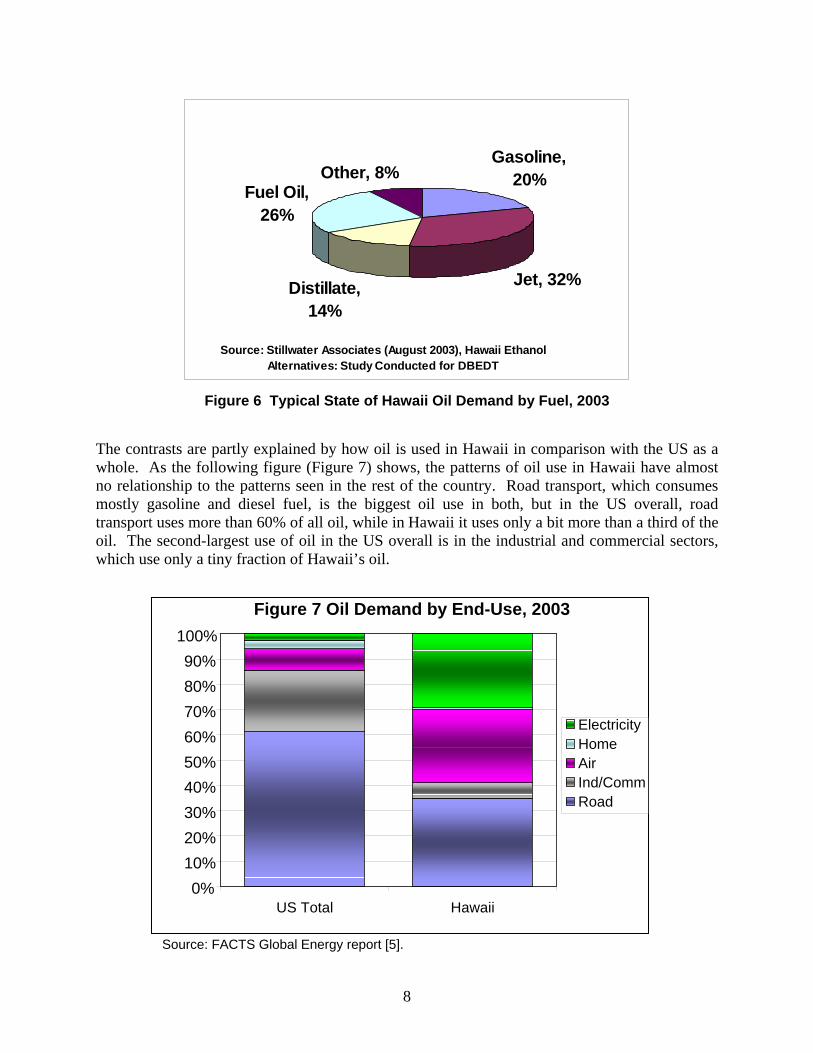
Source: Stillwater Associates (August 2003), Hawaii Ethanol Alternatives: Study Conducted for DBEDT

Gasoline, 20%

Jet, 32%Distillate, 14%

Fuel Oil, 26%

Other, 8%

Figure 6 Typical State of Hawaii Oil Demand by Fuel, 2003

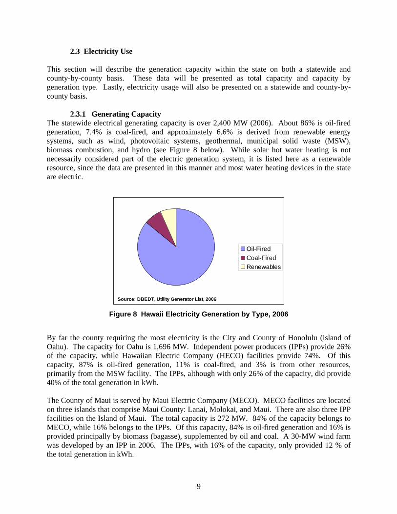
The contrasts are partly explained by how oil is used in Hawaii in comparison with the US as a whole. As the following figure (Figure 7) shows, the patterns of oil use in Hawaii have almost no relationship to the patterns seen in the rest of the country. Road transport, which consumes mostly gasoline and diesel fuel, is the biggest oil use in both, but in the US overall, road transport uses more than 60% of all oil, while in Hawaii it uses only a bit more than a third of the oil. The second-largest use of oil in the US overall is in the industrial and commercial sectors, which use only a tiny fraction of Hawaii’s oil.

Figure 7 Oil Demand by End-Use, 2003

0%

ElectricityHome AirInd/Comm Road

HawaiiUS Total

100% 90% 80% 70% 60% 50% 40% 30% 20% 10%

Source: FACTS Global Energy report [5].

8

2.3 Electricity Use This section will describe the generation capacity within the state on both a statewide and county-by-county basis. These data will be presented as total capacity and capacity by generation type. Lastly, electricity usage will also be presented on a statewide and county-by-county basis.

2.3.1 Generating Capacity

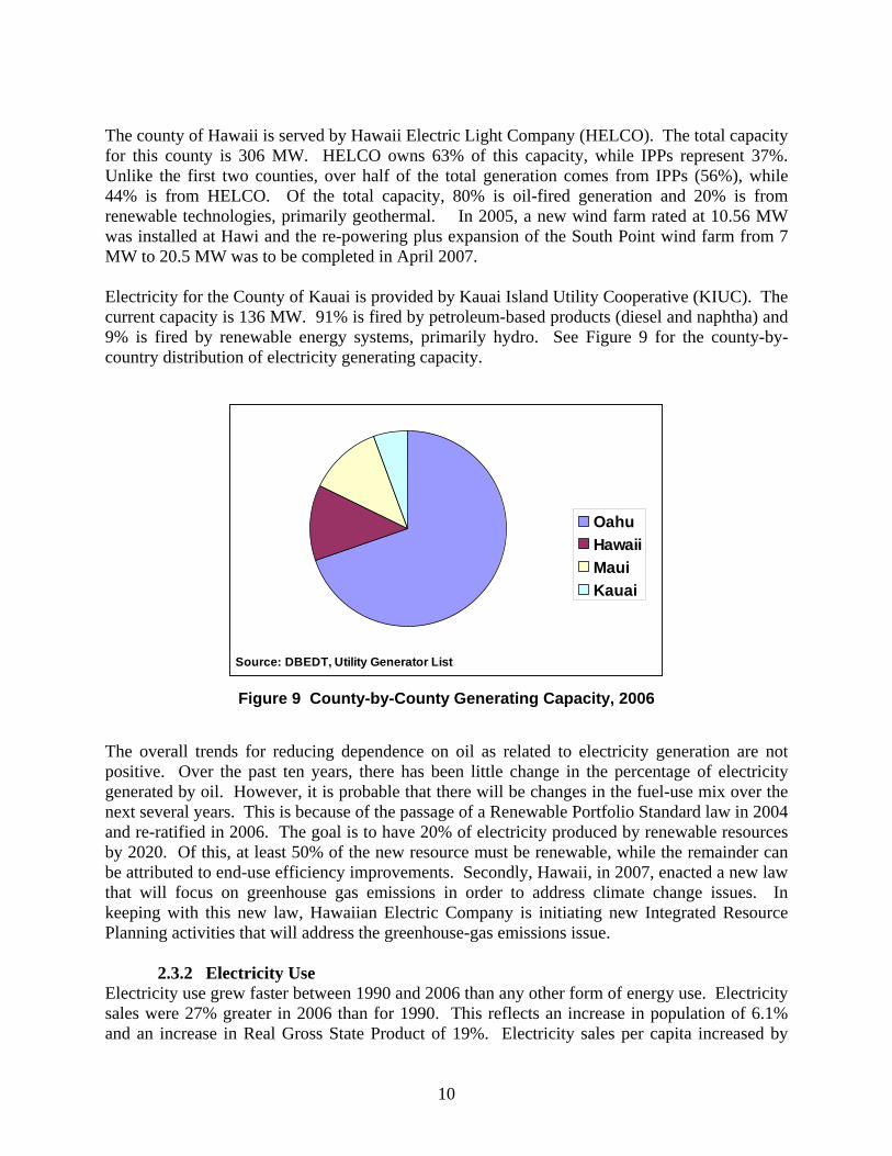
The statewide electrical generating capacity is over 2,400 MW (2006). About 86% is oil-fired generation, 7.4% is coal-fired, and approximately 6.6% is derived from renewable energy systems, such as wind, photovoltaic systems, geothermal, municipal solid waste (MSW), biomass combustion, and hydro (see Figure 8 below). While solar hot water heating is not necessarily considered part of the electric generation system, it is listed here as a renewable resource, since the data are presented in this manner and most water heating devices in the state are electric.

Source: DBEDT, Utility Generator List, 2006

Oil-FiredCoal-FiredRenewables

Figure 8 Hawaii Electricity Generation by Type, 2006

By far the county requiring the most electricity is the City and County of Honolulu (island of Oahu). The capacity for Oahu is 1,696 MW. Independent power producers (IPPs) provide 26% of the capacity, while Hawaiian Electric Company (HECO) facilities provide 74%. Of this capacity, 87% is oil-fired generation, 11% is coal-fired, and 3% is from other resources, primarily from the MSW facility. The IPPs, although with only 26% of the capacity, did provide 40% of the total generation in kWh. The County of Maui is served by Maui Electric Company (MECO). MECO facilities are located on three islands that comprise Maui County: Lanai, Molokai, and Maui. There are also three IPP facilities on the Island of Maui. The total capacity is 272 MW. 84% of the capacity belongs to MECO, while 16% belongs to the IPPs. Of this capacity, 84% is oil-fired generation and 16% is provided principally by biomass (bagasse), supplemented by oil and coal. A 30-MW wind farm was developed by an IPP in 2006. The IPPs, with 16% of the capacity, only provided 12 % of the total generation in kWh.

9

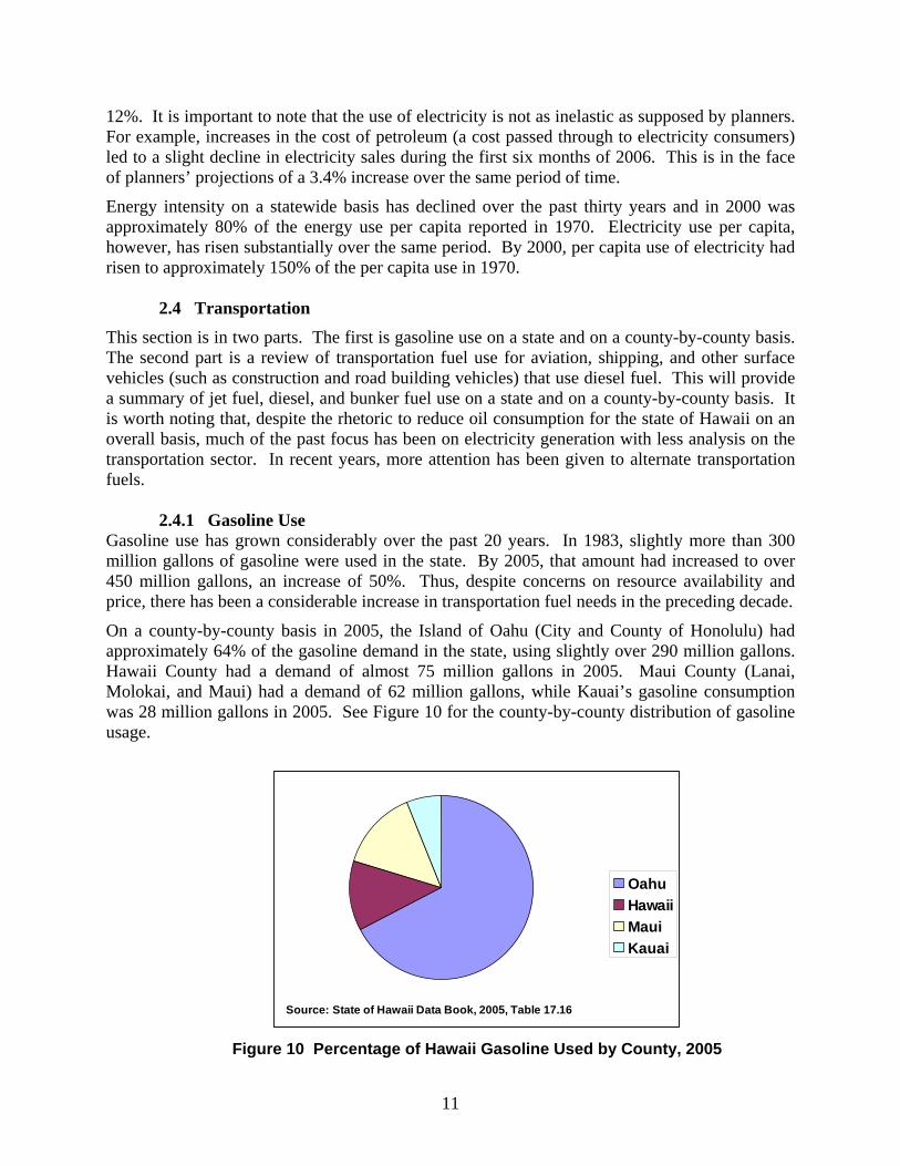
The county of Hawaii is served by Hawaii Electric Light Company (HELCO). The total capacity for this county is 306 MW. HELCO owns 63% of this capacity, while IPPs represent 37%. Unlike the first two counties, over half of the total generation comes from IPPs (56%), while 44% is from HELCO. Of the total capacity, 80% is oil-fired generation and 20% is from renewable technologies, primarily geothermal. In 2005, a new wind farm rated at 10.56 MW was installed at Hawi and the re-powering plus expansion of the South Point wind farm from 7 MW to 20.5 MW was to be completed in April 2007. Electricity for the County of Kauai is provided by Kauai Island Utility Cooperative (KIUC). The current capacity is 136 MW. 91% is fired by petroleum-based products (diesel and naphtha) and 9% is fired by renewable energy systems, primarily hydro. See Figure 9 for the county-by-country distribution of electricity generating capacity.

Source: DBEDT, Utility Generator List

OahuHawaiiMauiKauai

Figure 9 County-by-County Generating Capacity, 2006

The overall trends for reducing dependence on oil as related to electricity generation are not positive. Over the past ten years, there has been little change in the percentage of electricity generated by oil. However, it is probable that there will be changes in the fuel-use mix over the next several years. This is because of the passage of a Renewable Portfolio Standard law in 2004 and re-ratified in 2006. The goal is to have 20% of electricity produced by renewable resources by 2020. Of this, at least 50% of the new resource must be renewable, while the remainder can be attributed to end-use efficiency improvements. Secondly, Hawaii, in 2007, enacted a new law that will focus on greenhouse gas emissions in order to address climate change issues. In keeping with this new law, Hawaiian Electric Company is initiating new Integrated Resource Planning activities that will address the greenhouse-gas emissions issue.

2.3.2 Electricity Use Electricity use grew faster between 1990 and 2006 than any other form of energy use. Electricity sales were 27% greater in 2006 than for 1990. This reflects an increase in population of 6.1% and an increase in Real Gross State Product of 19%. Electricity sales per capita increased by

10

12%. It is important to note that the use of electricity is not as inelastic as supposed by planners. For example, increases in the cost of petroleum (a cost passed through to electricity consumers) led to a slight decline in electricity sales during the first six months of 2006. This is in the face of planners’ projections of a 3.4% increase over the same period of time.

Energy intensity on a statewide basis has declined over the past thirty years and in 2000 was approximately 80% of the energy use per capita reported in 1970. Electricity use per capita, however, has risen substantially over the same period. By 2000, per capita use of electricity had risen to approximately 150% of the per capita use in 1970.

2.4 Transportation

This section is in two parts. The first is gasoline use on a state and on a county-by-county basis. The second part is a review of transportation fuel use for aviation, shipping, and other surface vehicles (such as construction and road building vehicles) that use diesel fuel. This will provide a summary of jet fuel, diesel, and bunker fuel use on a state and on a county-by-county basis. It is worth noting that, despite the rhetoric to reduce oil consumption for the state of Hawaii on an overall basis, much of the past focus has been on electricity generation with less analysis on the transportation sector. In recent years, more attention has been given to alternate transportation fuels. 2.4.1 Gasoline Use Gasoline use has grown considerably over the past 20 years. In 1983, slightly more than 300 million gallons of gasoline were used in the state. By 2005, that amount had increased to over 450 million gallons, an increase of 50%. Thus, despite concerns on resource availability and price, there has been a considerable increase in transportation fuel needs in the preceding decade.

On a county-by-county basis in 2005, the Island of Oahu (City and County of Honolulu) had approximately 64% of the gasoline demand in the state, using slightly over 290 million gallons. Hawaii County had a demand of almost 75 million gallons in 2005. Maui County (Lanai, Molokai, and Maui) had a demand of 62 million gallons, while Kauai’s gasoline consumption was 28 million gallons in 2005. See Figure 10 for the county-by-county distribution of gasoline usage.

Source: State of Hawaii Data Book, 2005, Table 17.16

OahuHawaiiMauiKauai

Figure 10 Percentage of Hawaii Gasoline Used by County, 2005

11

2.4.2 Other Petroleum Products for Transportation Unlike all of the other states in the country, Hawaii has a substantively different usage mix for transportation fuels. In particular, the percentage of fuel used for air travel is significantly greater than that for other states. Similarly, its location in the middle of the Pacific Ocean requires a considerable amount of materials to be shipped in and out of the state via marine transportation. Thus, bunker fuel usage on a state per-capita or GSP basis is greater than for most other states, including coastal states. Total jet fuel consumption was 7.7 million barrels in 2005. As discussed in Section 2.2, this amounted to approximately 30% of the petroleum use in the state. This compares to approximately 10% of petroleum use on a nation-wide basis. This consumption includes jet fuel refined in the state and refined product shipped directly into the state. Oahu consumed 69% of the jet-fuel total, Maui 19%, Hawaii County 8.5%, and Kauai 3.6%. In addition to the Mainland and international flights leaving Honolulu, airliners flying inter-island routes are re-fueled only in Honolulu, based on discussions with airport officials as part of a different part of the program. Total diesel use amounted to approximately 4.5 million barrels per year (2005). This is approximately 20% of the total petroleum use in the state. Oahu accounts for 71% of the total diesel fuel usage, Hawaii County 11%, Kauai 11%, and Maui 7%. As described in earlier sections, a considerable amount of residual fuel oil results from refinery operations. While most of this is utilized for electricity generation, approximately 10% is used as bunker fuel for marine shipping. This is significant in that approximately 25% of petroleum usage in the state is residual fuel oil as compared to the national average of 5% [5]. A small amount of liquefied petroleum gas (LPG) is used for transportation (some City and County of Honolulu vehicles), but this amounts to less than 0.1% of all petroleum liquids. LPG use in buildings will be discussed in the next section.

2.5 Petroleum Product Use in Buildings

This section covers fuels (i.e., LPG and synthetic natural gas – SNG) that are used in buildings for a variety of purposes, such as water heating, cooking, space heating, and absorption chilling. The total statewide usage of these fuels in 2005 amounted to an equivalent of about 3.1 trillion Btu, with 93% of this total coming from SNG, which is consumed only on Oahu. The SNG usage would be equivalent to about 21 million gallons of diesel fuel (using a standard value of 139,000 Btu/gallon of diesel) and this would be equal to just over 2% of all petroleum liquids. Due to Hawaii’s location, these fuel types are used to a much lesser degree as compared to the rest of the country. This is also due to the fact that, since there are no natural gas pipelines as in the continental United States, certain functions that use natural gas on the Mainland, such as water heating, frequently use electricity in Hawaii. Further, a considerable number of solar water heating systems have also been deployed in the state. Thus, the percentage of the use of these fuel types is much lower (about 2% of total energy consumption) versus the nation as a whole (over 15%).

12

2.6 Other Energy-related Activities and Products from State-Based Refineries The summary of petroleum product usage is not complete unless products that are used for economic activities other than energy systems are included. Other products are also produced in the state-based refineries that are extremely important to the state’s economy. Two of these products are liquid asphalt and lubricants. In fuel-use models employed by the state, two metrics are given for calculating the production of these materials in a manner consistent with that for energy products. The total number of barrels of petroleum used for the production of asphalt and lubricants is almost 450,000 barrels per year. This is slightly less than 1% of overall imports. In a similar manner, calculations done on a Btu basis also show that approximately 1% of the oil usage goes to the production of these materials. While this is a small percentage, closure of the state-based refineries would potentially lead to significant problems in the construction and road-building sectors should these products not be available locally. 3.0 Analysis of Petroleum Price Impacts on the State Economy A considerable body of literature is available for evaluating the most reasonable methodology for evaluating projected impacts to the economy based on the volatility and/or the long-term increase in petroleum prices. The extensive background that supports the following analyses is presented in “Analysis of the Impact of Petroleum Prices on the State of Hawaii’s Economy” by M. Coffman et al. This paper was developed as part of this overall Section 355 Study. Specific to Hawaii’s situation, Gopalakrishnan, Tian, and Tran [6] studied the impact of oil price shocks on Hawaii’s economy from 1974 to 1986 using an econometric vector auto-regression model. Their model looks at the effect of changing oil prices on several national variables (interest rates and real GNP) as well as several local variables (local prices, total civilian labor force, and real personal income). Similar to other analyses in this area, Gopalakrishnan et. al. find that initial impacts are more intense and dissipate over time. On a national level, they find that oil price shocks have negative effects on interest rates and real GNP. Locally, oil price shocks are found to have an immediate inflationary effect, although this effect lessens considerably over time. Real personal income similarly decreases rapidly and then normalizes. An interesting and somewhat counter-intuitive finding is that oil price shocks increase employment, at least initially. Gopalakrishnan et al. explain that this result “lies in factor substitution occurring in different sectors of Hawaii’s economy, leading to the replacement of energy-intensive practices by labor-intensive ones” [6, p. 304]. The shift of Hawaii’s economy away from agriculture and towards service-related industries may change this result in future analyses. Hawaii’s geographically remote nature and tourism-dependent economy make service-sectors highly (indirectly) oil-dependent and unlikely to substitute energy with labor.

3.1 Data Sources for the Economic Analyses To assess the economic effects on Hawaii’s economy of increasing oil prices over time, a number of inputs to the UHERO models of the State economy were required. The main dataset used to calibrate the model is based on the DBEDT 1997 Hawaii State Input-Output (I-O) Study.1 The State of Hawaii I-O Table has been updated to reflect information from the 2000 1 Although an updated 2002 table exists, this dataset was not used for two reasons. The first is that the 2002 I-O table is much less in-depth (with only 67 sectors) and the specific industries targeted in the analysis, namely petroleum manufacturing and the electric sector, are not entirely represented. Also, in an earlier paper for the 355

13

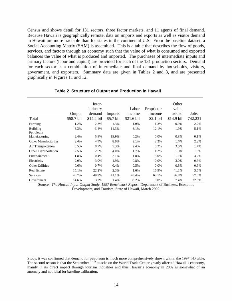
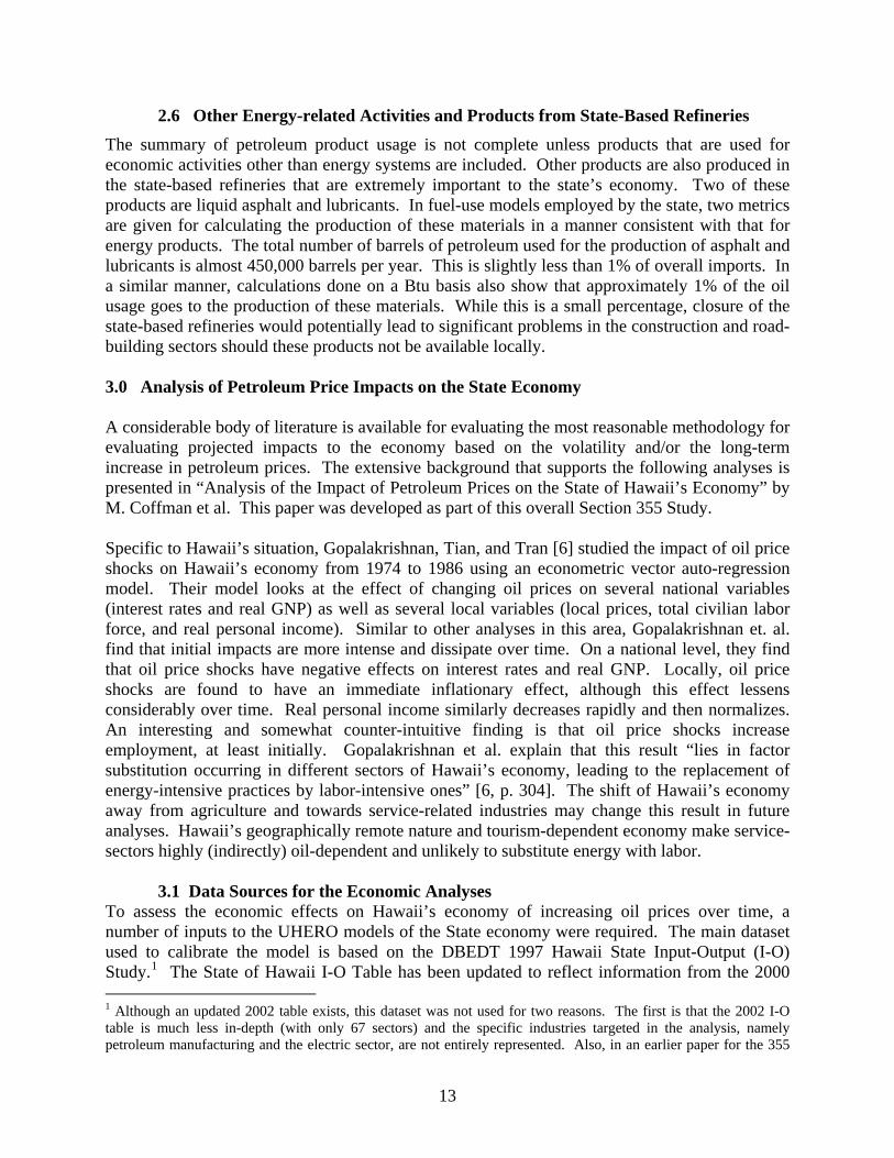
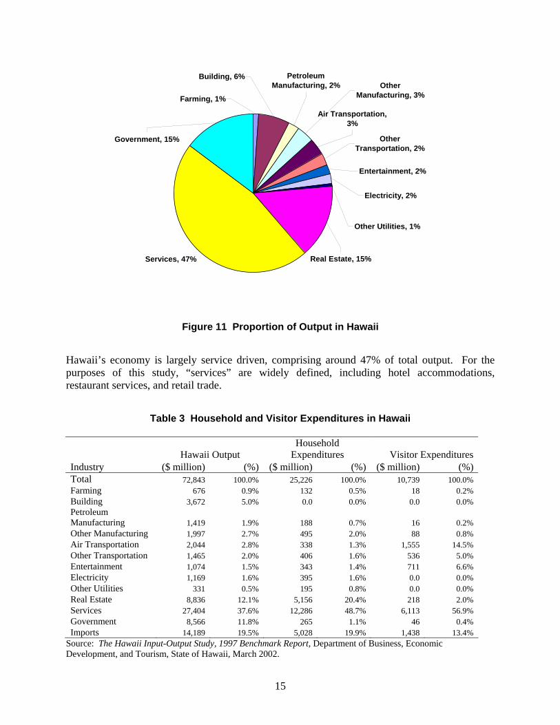
Census and shows detail for 131 sectors, three factor markets, and 11 agents of final demand. Because Hawaii is geographically remote, data on imports and exports as well as visitor demand in Hawaii are more tractable than for states in the continental U.S. From the baseline dataset, a Social Accounting Matrix (SAM) is assembled. This is a table that describes the flow of goods, services, and factors through an economy such that the value of what is consumed and exported balances the value of what is produced and imported. The purchases of intermediate inputs and primary factors (labor and capital) are provided for each of the 131 production sectors. Demand for each sector is a combination of intermediate and final demand by households, visitors, government, and exporters. Summary data are given in Tables 2 and 3, and are presented graphically in Figures 11 and 12.

Table 2 Structure of Output and Production in Hawaii

Output

Inter-industry demand Imports

Labor income

Proprietor income

Other value added Jobs

Total $58.7 bil $14.4 bil $5.7 bil $21.6 bil $2.1 bil $14.9 bil 742,231Farming 1.2% 2.3% 1.3% 1.0% 1.3% 0.9% 2.2% Building 6.3% 3.4% 11.3% 6.1% 12.1% 1.9% 5.1% Petroleum Manufacturing 2.4% 5.8% 19.9% 0.2% 0.0% 0.8% 0.1% Other Manufacturing 3.4% 4.9% 8.9% 2.1% 2.2% 1.6% 2.3% Air Transportation 3.5% 0.7% 5.3% 2.4% 0.3% 3.5% 1.4% Other Transportation 2.5% 2.5% 4.0% 1.7% 1.2% 1.3% 1.9% Entertainment 1.8% 0.4% 2.1% 1.8% 3.0% 1.1% 3.2% Electricity 2.0% 3.9% 1.9% 0.8% 0.0% 3.0% 0.3% Other Utilities 0.6% 0.7% 0.4% 0.5% 0.0% 0.8% 0.3% Real Estate 15.1% 22.2% 2.3% 1.6% 16.9% 41.1% 3.6% Services 46.7% 49.9% 41.1% 48.4% 63.1% 36.8% 57.5% Government 14.6% 3.2% 1.4% 33.2% 0.0% 7.4% 22.0%

Source: The Hawaii Input-Output Study, 1997 Benchmark Report, Department of Business, Economic Development, and Tourism, State of Hawaii, March 2002.

Study, it was confirmed that demand for petroleum is much more comprehensively shown within the 1997 I-O table. The second reason is that the September 11th attacks on the World Trade Center greatly affected Hawaii’s economy, mainly in its direct impact through tourism industries and thus Hawaii’s economy in 2002 is somewhat of an anomaly and not ideal for baseline calibration.

14

Services, 47%

Other Transportation, 2%

Entertainment, 2%

Air Transportation, 3%

Other Manufacturing, 3%

Petroleum Manufacturing, 2%

Building, 6%

Farming, 1%

Government, 15%

Electricity, 2%

Other Utilities, 1%

Real Estate, 15%

Figure 11 Proportion of Output in Hawaii

Hawaii’s economy is largely service driven, comprising around 47% of total output. For the purposes of this study, “services” are widely defined, including hotel accommodations, restaurant services, and retail trade.

Table 3 Household and Visitor Expenditures in Hawaii

Hawaii Output Household

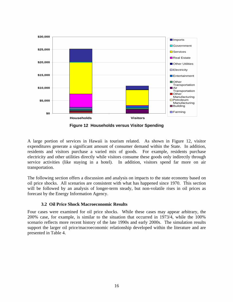
Expenditures Visitor ExpendituresIndustry ($ million) (%) ($ million) (%) ($ million) (%)Total 72,843 100.0% 25,226 100.0% 10,739 100.0% Farming 676 0.9% 132 0.5% 18 0.2% Building 3,672 5.0% 0.0 0.0% 0.0 0.0% Petroleum Manufacturing 1,419 1.9% 188 0.7% 16 0.2% Other Manufacturing 1,997 2.7% 495 2.0% 88 0.8% Air Transportation 2,044 2.8% 338 1.3% 1,555 14.5% Other Transportation 1,465 2.0% 406 1.6% 536 5.0% Entertainment 1,074 1.5% 343 1.4% 711 6.6% Electricity 1,169 1.6% 395 1.6% 0.0 0.0% Other Utilities 331 0.5% 195 0.8% 0.0 0.0% Real Estate 8,836 12.1% 5,156 20.4% 218 2.0% Services 27,404 37.6% 12,286 48.7% 6,113 56.9% Government 8,566 11.8% 265 1.1% 46 0.4% Imports 14,189 19.5% 5,028 19.9% 1,438 13.4%

Source: The Hawaii Input-Output Study, 1997 Benchmark Report, Department of Business, Economic Development, and Tourism, State of Hawaii, March 2002.

15

$0

$5,000

$10,000

$15,000

$20,000

$25,000

$30,000

Households Visitors

Imports

Government

Services

Real Estate

Other Utilities

Electricity

Entertainment

OtherTransportationAirTransportationOtherManufacturingPetroleumManufacturingBuilding

Farming

Figure 12 Households versus Visitor Spending

A large portion of services in Hawaii is tourism related. As shown in Figure 12, visitor expenditures generate a significant amount of consumer demand within the State. In addition, residents and visitors purchase a varied mix of goods. For example, residents purchase electricity and other utilities directly while visitors consume these goods only indirectly through service activities (like staying in a hotel). In addition, visitors spend far more on air transportation.

The following section offers a discussion and analysis on impacts to the state economy based on oil price shocks. All scenarios are consistent with what has happened since 1970. This section will be followed by an analysis of longer-term steady, but non-volatile rises in oil prices as forecast by the Energy Information Agency.

3.2 Oil Price Shock Macroeconomic Results

Four cases were examined for oil price shocks. While these cases may appear arbitrary, the 200% case, for example, is similar to the situation that occurred in 1973/4, while the 100% scenario reflects more recent history of the late 1990s and early 2000s. The simulation results support the larger oil price/macroeconomic relationship developed within the literature and are presented in Table 4.

16

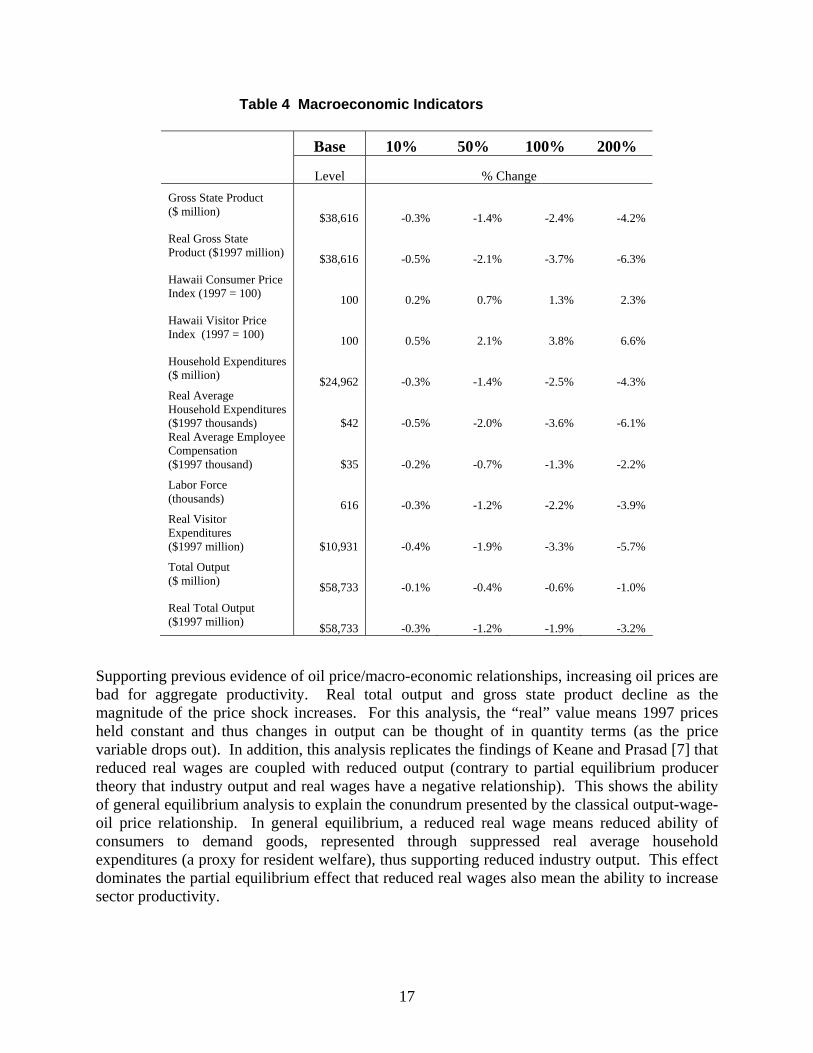
Table 4 Macroeconomic Indicators

Base 10% 50% 100% 200% Level % Change Gross State Product ($ million) $38,616 -0.3% -1.4% -2.4% -4.2%

Real Gross State Product ($1997 million) $38,616 -0.5% -2.1% -3.7% -6.3%

Hawaii Consumer Price Index (1997 = 100) 100 0.2% 0.7% 1.3% 2.3%

Hawaii Visitor Price Index (1997 = 100) 100 0.5% 2.1% 3.8% 6.6%

Household Expenditures ($ million) $24,962 -0.3% -1.4% -2.5% -4.3% Real Average Household Expenditures ($1997 thousands) $42 -0.5% -2.0% -3.6% -6.1% Real Average Employee Compensation ($1997 thousand) $35 -0.2% -0.7% -1.3% -2.2%

Labor Force (thousands) 616 -0.3% -1.2% -2.2% -3.9% Real Visitor Expenditures ($1997 million) $10,931 -0.4% -1.9% -3.3% -5.7%

Total Output ($ million) $58,733 -0.1% -0.4% -0.6% -1.0%

Real Total Output ($1997 million) $58,733 -0.3% -1.2% -1.9% -3.2%

Supporting previous evidence of oil price/macro-economic relationships, increasing oil prices are bad for aggregate productivity. Real total output and gross state product decline as the magnitude of the price shock increases. For this analysis, the “real” value means 1997 prices held constant and thus changes in output can be thought of in quantity terms (as the price variable drops out). In addition, this analysis replicates the findings of Keane and Prasad [7] that reduced real wages are coupled with reduced output (contrary to partial equilibrium producer theory that industry output and real wages have a negative relationship). This shows the ability of general equilibrium analysis to explain the conundrum presented by the classical output-wage-oil price relationship. In general equilibrium, a reduced real wage means reduced ability of consumers to demand goods, represented through suppressed real average household expenditures (a proxy for resident welfare), thus supporting reduced industry output. This effect dominates the partial equilibrium effect that reduced real wages also mean the ability to increase sector productivity.

17

These results are also what one would intuitively expect. Since crude oil is an import and a factor of production, when its price increases, this causes an increase in production costs and the costs of goods; hence demand falls and there is loss of output and hence loss of jobs.

Unlike Gopalakrishnan et al. [6], oil prices increases lead to increased unemployment in the State. This could result from structural changes in the economy since Gopalakrishnan et al.’s study was conducted and also because of the assumption that the shock occurs in the short-run.

The Consumer Price Index (CPI), which represents the composite price of the basket of residential consumer goods (better thought of as the Resident Price Index), is less inflationary than the Visitor Price Index (VPI). This shows how visitor consumption patterns are more oil-intensive than resident consumption patterns, particularly in the consumption of air travel.

There is an overall inflationary effect shown through the CPI, supporting the econometric literature. There are, however, competing deflationary effects caused by an increase in world oil prices. The primary and dominant effect is inflationary, occurring from an exogenous price increase in a factor of production. A competing deflationary effect is that an increase in world oil prices leads to a reduction in real visitor expenditures. Visitor expenditures have an inflationary effect within an economy because they act as an exogenous infusion of dollars within the State. Increased oil prices mean that traveling to and visiting Hawaii becomes more expensive in real terms (as represented by a rising VPI) and visitors purchase relatively less (as represented by decreasing real visitor expenditures).2 While this has other welfare impacts, particularly on industry demand, it also has this deflationary aspect. The second competing effect, stems from consumers (residents and visitors) shifting demand away from petroleum-intensive sectors (see Table 8 and 9). Resident welfare, as represented through real average household expenditures, decreases under all scenarios. This means that the inflationary effect dominates throughout. This finding suggests the presence of a “threshold” [8].

3.2.1 Sector Level Results Table 5 shows output levels in constant 1997 prices for farming, building, petroleum manufacturing, other manufacturing, air transportation, other transportation, entertainment, real estate & rentals, electricity, other utilities, services and government in the “Base” case as well as the “% change from the Base” case for each oil price shock scenario. As expected, an increase in the world price of crude oil has the largest effect on the petroleum manufacturing industry (the sector which directly absorbs the shock within the model).3

2 The static model presented does not consider global effects. In reality, an increase in world oil prices would affect nominal visitor expenditures. This would have an even larger impact on real visitor expenditures than presented above. A simulation that assumes decreased nominal visitor expenditures in Hawaii under each oil price scenario was run, where larger oil price shocks meant less nominal visitor expenditures. The results reinforce the premise that visitor expenditures are inflationary within Hawaii’s economy and decreased nominal visitor expenditures similarly have deflationary effects, which would further decrease Hawaii’s CPI. There are, of course, other negative effects on Hawaii’s economy, particularly debilitating to visitor-related sectors. 3 The Hawaii CGE model assumes homogeneous products within sectors. This means it does not consider the impact of differentiated products within the petroleum manufacturing industry. For example, the petroleum manufacturing sector sells jet fuel to the airline industry, gasoline to the transportation industry, and residual fuel oil to the electric sector. The production function of petroleum manufacturing in reality does not smoothly transition from serving the air transportation market to the electricity market but is rather constrained by differentiated products where residual fuel oil is a byproduct of jet fuel production.

18

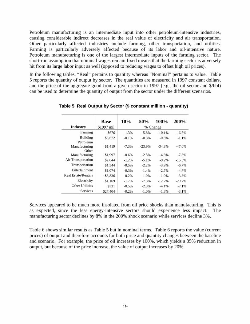
Petroleum manufacturing is an intermediate input into other petroleum-intensive industries, causing considerable indirect decreases in the real value of electricity and air transportation. Other particularly affected industries include farming, other transportation, and utilities. Farming is particularly adversely affected because of its labor and oil-intensive nature. Petroleum manufacturing is one of the largest intermediate inputs of the farming sector. The short-run assumption that nominal wages remain fixed means that the farming sector is adversely hit from its large labor input as well (opposed to reducing wages to offset high oil prices).

In the following tables, “Real” pertains to quantity whereas “Nominal” pertains to value. Table 5 reports the quantity of output by sector. The quantities are measured in 1997 constant dollars, and the price of the aggregate good from a given sector in 1997 (e.g., the oil sector and $/bbl) can be used to determine the quantity of output from the sector under the different scenarios.

Table 5 Real Output by Sector ($ constant million - quantity)

Base 10% 50% 100% 200% Industry $1997 mil % Change

Farming $676 -1.3% -5.8% -10.1% -16.5% Building $3,672 -0.1% -0.3% -0.6% -1.1%

Petroleum Manufacturing $1,419 -7.3% -23.9% -34.8% -47.0%

Other Manufacturing $1,997 -0.6% -2.5% -4.6% -7.8%

Air Transportation $2,044 -1.2% -5.1% -9.2% -15.5% Transportation $1,544 -0.5% -2.2% -3.9% -6.7% Entertainment $1,074 -0.3% -1.4% -2.7% -4.7%

Real Estate/Rentals $8,836 -0.2% -1.0% -1.9% -3.3% Electricity $1,169 -1.7% -7.3% -12.7% -20.7%

Other Utilities $331 -0.5% -2.3% -4.1% -7.1% Services $27,404 -0.2% -1.0% -1.8% -3.1%

Services appeared to be much more insolated from oil price shocks than manufacturing. This is as expected, since the less energy-intensive sectors should experience less impact. The manufacturing sector declines by 8% in the 200% shock scenario while services decline 3%.

Table 6 shows similar results as Table 5 but in nominal terms. Table 6 reports the value (current prices) of output and therefore accounts for both price and quantity changes between the baseline and scenario. For example, the price of oil increases by 100%, which yields a 35% reduction in output, but because of the price increase, the value of output increases by 20%.

19

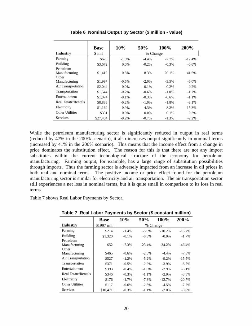
Table 6 Nominal Output by Sector ($ million - value)

Base 10% 50% 100% 200% Industry $ mil % Change Farming $676 -1.0% -4.4% -7.7% -12.4% Building $3,672 0.0% -0.2% -0.3% -0.6% Petroleum Manufacturing $1,419 0.5% 8.3% 20.1% 41.5% Other Manufacturing $1,997 -0.5% -2.0% -3.5% -6.0% Air Transportation $2,044 0.0% -0.1% -0.2% -0.2% Transportation $1,544 -0.2% -0.6% -1.0% -1.7% Entertainment $1,074 -0.1% -0.3% -0.6% -1.1% Real Estate/Rentals $8,836 -0.2% -1.0% -1.8% -3.1% Electricity $1,169 0.9% 4.3% 8.2% 15.3% Other Utilities $331 0.0% 0.0% 0.1% 0.3% Services $27,404 -0.2% -0.7% -1.3% -2.2%

While the petroleum manufacturing sector is significantly reduced in output in real terms (reduced by 47% in the 200% scenario), it also increases output significantly in nominal terms (increased by 41% in the 200% scenario). This means that the income effect from a change in price dominates the substitution effect. The reason for this is that there are not any import substitutes within the current technological structure of the economy for petroleum manufacturing. Farming output, for example, has a large range of substitution possibilities through imports. Thus the farming sector is adversely impacted from an increase in oil prices in both real and nominal terms. The positive income or price effect found for the petroleum manufacturing sector is similar for electricity and air transportation. The air transportation sector still experiences a net loss in nominal terms, but it is quite small in comparison to its loss in real terms.

Table 7 shows Real Labor Payments by Sector.

Table 7 Real Labor Payments by Sector ($ constant million) Base 10% 50% 100% 200% Industry $1997 mil % Change Farming $214 -1.4% -5.9% -10.2% -16.7% Building $1,320 -0.1% -0.5% -0.9% -1.7% Petroleum Manufacturing $52 -7.3% -23.4% -34.2% -46.4% Other Manufacturing $465 -0.6% -2.5% -4.4% -7.5% Air Transportation $527 -1.2% -5.2% -9.2% -15.5% Transportation $371 -0.5% -2.2% -3.9% -6.7% Entertainment $393 -0.4% -1.6% -2.9% -5.1% Real Estate/Rentals $346 -0.3% -1.1% -2.0% -3.5% Electricity $176 -1.7% -7.3% -12.7% -20.7% Other Utilities $117 -0.6% -2.5% -4.5% -7.7% Services $10,471 -0.3% -1.1% -2.0% -3.6%

20

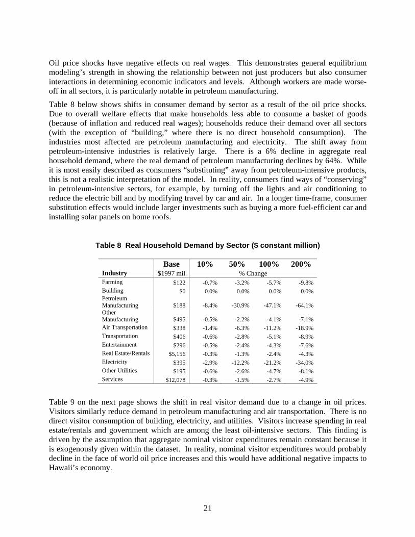
Oil price shocks have negative effects on real wages. This demonstrates general equilibrium modeling’s strength in showing the relationship between not just producers but also consumer interactions in determining economic indicators and levels. Although workers are made worse-off in all sectors, it is particularly notable in petroleum manufacturing.

Table 8 below shows shifts in consumer demand by sector as a result of the oil price shocks. Due to overall welfare effects that make households less able to consume a basket of goods (because of inflation and reduced real wages); households reduce their demand over all sectors (with the exception of “building,” where there is no direct household consumption). The industries most affected are petroleum manufacturing and electricity. The shift away from petroleum-intensive industries is relatively large. There is a 6% decline in aggregate real household demand, where the real demand of petroleum manufacturing declines by 64%. While it is most easily described as consumers “substituting” away from petroleum-intensive products, this is not a realistic interpretation of the model. In reality, consumers find ways of “conserving” in petroleum-intensive sectors, for example, by turning off the lights and air conditioning to reduce the electric bill and by modifying travel by car and air. In a longer time-frame, consumer substitution effects would include larger investments such as buying a more fuel-efficient car and installing solar panels on home roofs.

Table 8 Real Household Demand by Sector ($ constant million)

Base 10% 50% 100% 200% Industry $1997 mil % Change Farming $122 -0.7% -3.2% -5.7% -9.8% Building $0 0.0% 0.0% 0.0% 0.0% Petroleum Manufacturing $188 -8.4% -30.9% -47.1% -64.1% Other Manufacturing $495 -0.5% -2.2% -4.1% -7.1% Air Transportation $338 -1.4% -6.3% -11.2% -18.9% Transportation $406 -0.6% -2.8% -5.1% -8.9% Entertainment $296 -0.5% -2.4% -4.3% -7.6% Real Estate/Rentals $5,156 -0.3% -1.3% -2.4% -4.3% Electricity $395 -2.9% -12.2% -21.2% -34.0% Other Utilities $195 -0.6% -2.6% -4.7% -8.1% Services $12,078 -0.3% -1.5% -2.7% -4.9%

Table 9 on the next page shows the shift in real visitor demand due to a change in oil prices. Visitors similarly reduce demand in petroleum manufacturing and air transportation. There is no direct visitor consumption of building, electricity, and utilities. Visitors increase spending in real estate/rentals and government which are among the least oil-intensive sectors. This finding is driven by the assumption that aggregate nominal visitor expenditures remain constant because it is exogenously given within the dataset. In reality, nominal visitor expenditures would probably decline in the face of world oil price increases and this would have additional negative impacts to Hawaii’s economy.

21

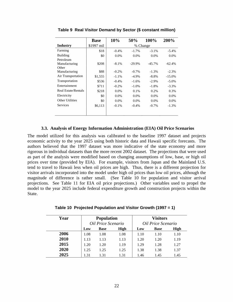
Table 9 Real Visitor Demand by Sector ($ constant million)

Base 10% 50% 100% 200% Industry $1997 mil % Change Farming $18 -0.4% -1.7% -3.1% -5.4% Building $0 0.0% 0.0% 0.0% 0.0% Petroleum Manufacturing $208 -8.1% -29.9% -45.7% -62.4% Other Manufacturing $88 -0.2% -0.7% -1.3% -2.3% Air Transportation $1,555 -1.1% -4.9% -8.8% -15.0% Transportation $536 -0.4% -1.6% -2.9% -5.0% Entertainment $711 -0.2% -1.0% -1.8% -3.3% Real Estate/Rentals $218 0.0% 0.1% 0.2% 0.3% Electricity $0 0.0% 0.0% 0.0% 0.0% Other Utilities $0 0.0% 0.0% 0.0% 0.0% Services $6,113 -0.1% -0.4% -0.7% -1.3%

3.3. Analysis of Energy Information Administration (EIA) Oil Price Scenarios The model utilized for this analysis was calibrated to the baseline 1997 dataset and projects economic activity to the year 2025 using both historic data and Hawaii specific forecasts. The authors believed that the 1997 dataset was more indicative of the state economy and more rigorous in individual datasets than the more recent 2002 dataset. The projections that were used as part of the analysis were modified based on changing assumptions of low, base, or high oil prices over time (provided by EIA). For example, visitors from Japan and the Mainland U.S. tend to travel to Hawaii less when oil prices are high. Thus, there is a different projection for visitor arrivals incorporated into the model under high oil prices than low oil prices, although the magnitude of difference is rather small. (See Table 10 for population and visitor arrival projections. See Table 11 for EIA oil price projections.) Other variables used to propel the model to the year 2025 include federal expenditure growth and construction projects within the State.

Table 10 Projected Population and Visitor Growth (1997 = 1)

Year Population Visitors Oil Price Scenario Oil Price Scenario Low Base High Low Base High

2006 1.08 1.08 1.08 1.10 1.10 1.10 2010 1.13 1.13 1.13 1.20 1.20 1.19 2015 1.20 1.20 1.19 1.29 1.28 1.27 2020 1.25 1.25 1.25 1.38 1.38 1.37 2025 1.31 1.31 1.31 1.46 1.45 1.45

22

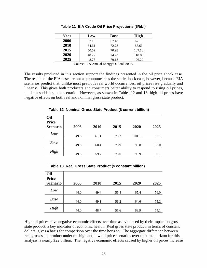
Table 11 EIA Crude Oil Price Projections ($/bbl)

Year Low Base High 2006 67.18 67.18 67.18 2010 64.61 72.78 87.66 2015 50.52 70.98 107.16 2020 48.77 74.23 118.89 2025 48.77 79.18 126.20

Source: EIA Annual Energy Outlook 2006. The results produced in this section support the findings presented in the oil price shock case. The results of the EIA case are not as pronounced as the static shock case, however, because EIA scenarios predict that, unlike most previous real world occurrences, oil prices rise gradually and linearly. This gives both producers and consumers better ability to respond to rising oil prices, unlike a sudden shock scenario. However, as shown in Tables 12 and 13, high oil prices have negative effects on both real and nominal gross state product.

Table 12 Nominal Gross State Product ($ current billion)

Oil Price Scenario 2006 2010 2015 2020 2025

Low 49.8 61.1 78.2 101.1 133.1

Base 49.8 60.4 76.9 99.8 132.0

High 49.8 59.7 76.0 98.9 130.1 Table 13 Real Gross State Product ($ constant billion)

Oil Price Scenario 2006 2010 2015 2020 2025

Low 44.0 49.4 56.8 65.4 76.0

Base 44.0 49.1 56.2 64.6 75.2

High 44.0 48.7 55.6 63.9 74.1

High oil prices have negative economic effects over time as evidenced by their impact on gross state product, a key indicator of economic health. Real gross state product, in terms of constant dollars, gives a basis for comparison over the time horizon. The aggregate difference between real gross state product under the high and low oil price scenarios over the time horizon for this analysis is nearly $22 billion. The negative economic effects caused by higher oil prices increase

23

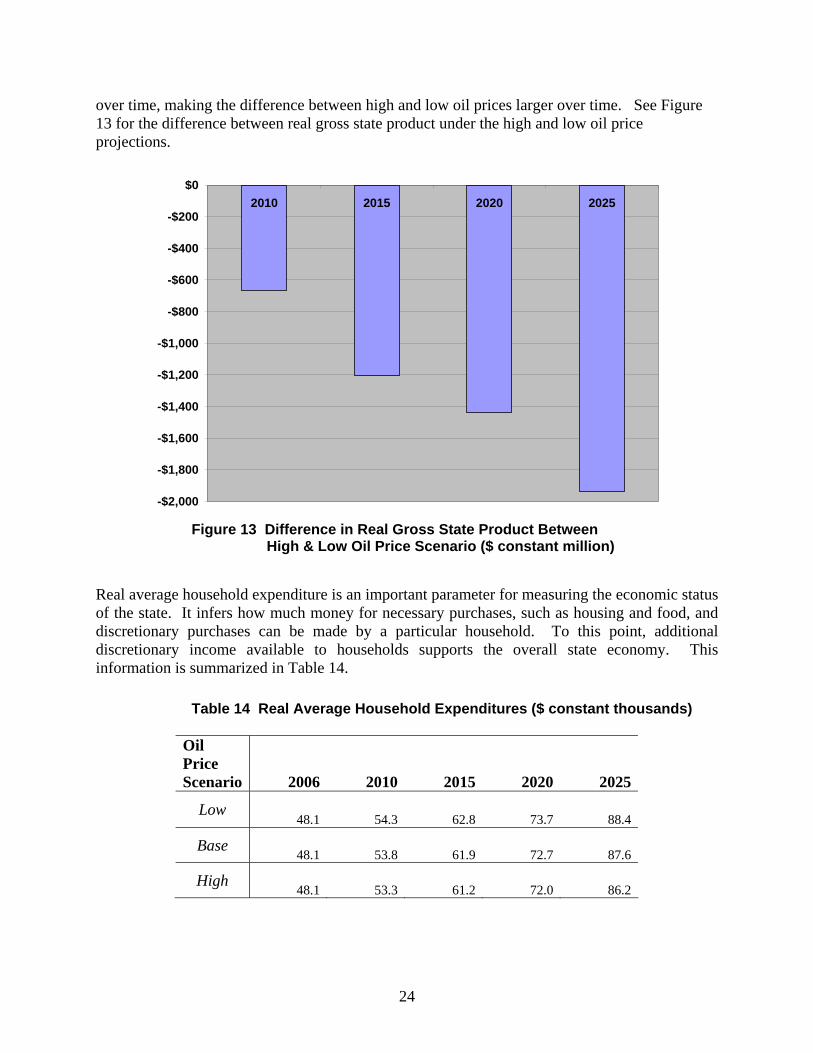
over time, making the difference between high and low oil prices larger over time. See Figure 13 for the difference between real gross state product under the high and low oil price projections.

-$2,000

-$1,800

-$1,600

-$1,400

-$1,200

-$1,000

-$800

-$600

-$400

-$200

$02010 2015 2020 2025

Figure 13 Difference in Real Gross State Product Between

High & Low Oil Price Scenario ($ constant million) Real average household expenditure is an important parameter for measuring the economic status of the state. It infers how much money for necessary purchases, such as housing and food, and discretionary purchases can be made by a particular household. To this point, additional discretionary income available to households supports the overall state economy. This information is summarized in Table 14.

Table 14 Real Average Household Expenditures ($ constant thousands)

Oil Price Scenario 2006 2010 2015 2020 2025

Low 48.1 54.3 62.8 73.7 88.4

Base 48.1 53.8 61.9 72.7 87.6

High 48.1 53.3 61.2 72.0 86.2

24

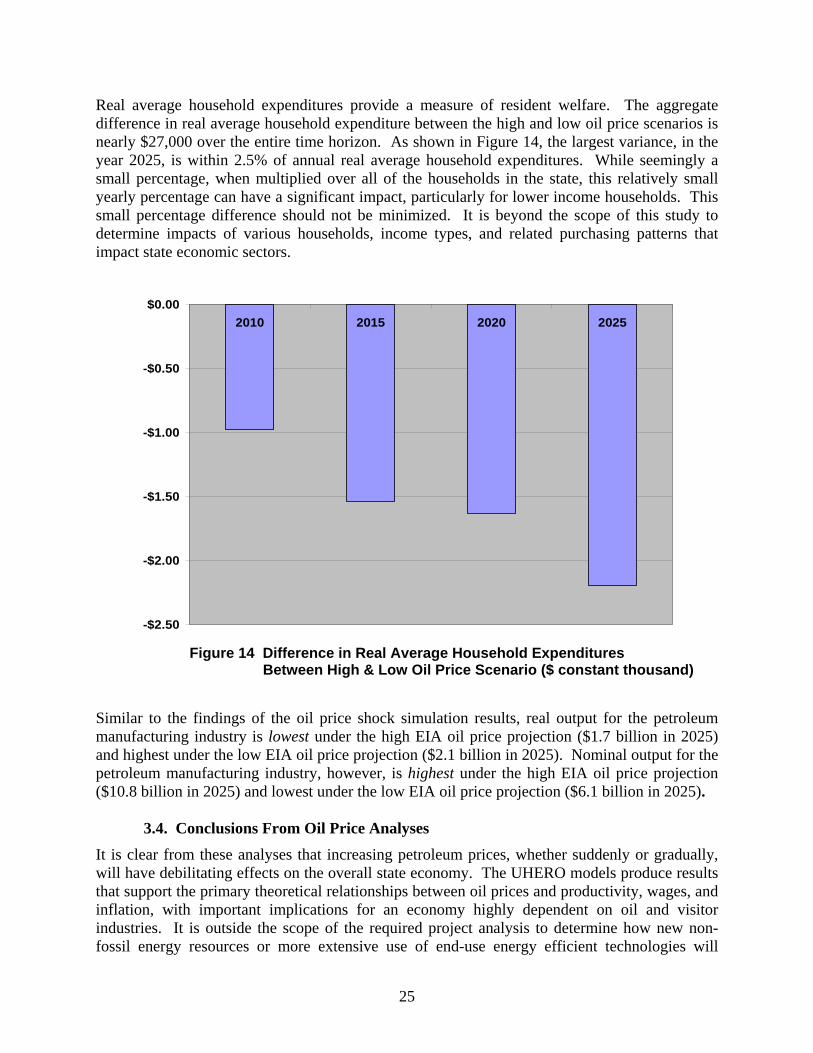
Real average household expenditures provide a measure of resident welfare. The aggregate difference in real average household expenditure between the high and low oil price scenarios is nearly $27,000 over the entire time horizon. As shown in Figure 14, the largest variance, in the year 2025, is within 2.5% of annual real average household expenditures. While seemingly a small percentage, when multiplied over all of the households in the state, this relatively small yearly percentage can have a significant impact, particularly for lower income households. This small percentage difference should not be minimized. It is beyond the scope of this study to determine impacts of various households, income types, and related purchasing patterns that impact state economic sectors.

-$2.50

-$2.00

-$1.50

-$1.00

-$0.50

$0.002010 2015 2020 2025

Figure 14 Difference in Real Average Household Expenditures

Between High & Low Oil Price Scenario ($ constant thousand)

Similar to the findings of the oil price shock simulation results, real output for the petroleum manufacturing industry is lowest under the high EIA oil price projection ($1.7 billion in 2025) and highest under the low EIA oil price projection ($2.1 billion in 2025). Nominal output for the petroleum manufacturing industry, however, is highest under the high EIA oil price projection ($10.8 billion in 2025) and lowest under the low EIA oil price projection ($6.1 billion in 2025).

3.4. Conclusions From Oil Price Analyses

It is clear from these analyses that increasing petroleum prices, whether suddenly or gradually, will have debilitating effects on the overall state economy. The UHERO models produce results that support the primary theoretical relationships between oil prices and productivity, wages, and inflation, with important implications for an economy highly dependent on oil and visitor industries. It is outside the scope of the required project analysis to determine how new non-fossil energy resources or more extensive use of end-use energy efficient technologies will

25

penetrate the market in the face of higher petroleum prices and serve to ease the burden placed on Hawaii’s economy by higher oil prices. The analyses of various oil price shock scenarios lead to a number of conclusions:

1). The oil price/macro-economic relationship developed in this analysis is consistent with econometric literature. That is, sudden oil price shocks decrease real productivity, decrease real wages across sectors, and are inflationary overall. In the 100% increase scenario, a doubling of world oil prices, real gross state product declines by 3.7%, real wages decline by 1.3%, and the Hawaii consumer price index rises by 1.3%.

2). While oil price shocks lead to inflationary pressure within an economy, both consumer demand shifts and the reduction in real visitor spending mean that oil price increases are associated with deflationary effects. The inflationary effect nonetheless dominates throughout all examined shock levels.

3). Oil price increases mean a direct reduction in real petroleum manufacturing output (a decline of 34% in the 100% scenario) yet an increase in nominal petroleum manufacturing output (an increase of 20% in the 100% scenario). This shows the income effect of a price increase dominates the substitution effect away from petroleum products.

4). Increased oil prices indirectly affect the electricity sector through intermediate purchases from the petroleum manufacturing industry. Electricity output declines in real terms (a decline of 13% in the 100% scenario) and increases in nominal terms (an increase of 8%). As with the petroleum manufacturing sector, the income effect of the price increase dominates the substitution effect away from petroleum products.

5). Output of air transportation declines by 9% in real terms and by 0.2% in nominal terms in the 100% scenario. This has an implicit impact on the tourism industry in the state.

Similar to the findings of Cunado and de Gracia [9], increasing oil prices have a larger effect in the short-run than the long-run. This analysis shows how oil price volatility has large real economic impacts. In the short-run, even a 10% increase in world oil prices can have negative real economic impacts, for instance a 0.5% decrease in real gross state product and a 0.16% increase in inflation.

Analyses of long-run impacts imply that the economy better adjusts, in comparison to the short-run price shocks, to changing oil prices in the high oil price EIA scenario. Increasing differences in oil prices over time between low and high cases have increasing negative effects on the economy. The largest difference occurs in the final year of analysis, 2025, with over a $2 billion difference in real gross state product between the high and low oil price scenarios. For Hawaii’s $70 billion dollar economy (measured in constant dollars as predicted for the year 2025), this is a sizable difference in economic performance due to a change in the price of a single factor of production, oil.

To conclude this section, it should be noted that there have been no refereed journal articles regarding recent oil price increases and Hawaii’s macroeconomic performance. From 2002 to 2006 world oil prices doubled, from $26 to $67 per barrel.4 Regular gasoline prices in Hawaii rose from roughly $1.80/gal to over $3.50/gal.5 However, Gross State Product has been growing 4 EIA data used for dynamic Hawaii CGE model. 5 http://www.hawaiigasprices.com/retail_price_chart.aspx

26

rapidly and unemployment was at a low of 2% in 2006. An updated econometric analysis similar to Gopalakrishnan et al. [6] could identify the recent relationship between rising oil prices and Hawaii’s economy. 4.0 Scenario Analyses Results Pursuant to language in Section 355 of EPACT, three scenarios were evaluated as to their feasibility and potential. These evaluations were followed by an attempt at analyzing the operational and economic impact to state-based refinery operations. These next sub-sections provide a summary of the results of these analyses.

4.1 Accelerated Use of Renewable Resources for Transportation Fuels This analysis is summarized from a report of the same title, by S. Turn et al., prepared as part of this overall study. Certain caveats are important to point out when considering the conclusions of this report. First, there is a reasonable amount of literature discussing the use of ethanol as a fuel. The basis for the analysis concerning ethanol is a recent report produced by HNEI for DBEDT [10]. The study relies on accepted literature and adds to the body of knowledge concerning ethanol use in the state.

The analysis for biodiesel, however, reflects the paucity of information currently available on the subject. For biodiesel, unlike for ethanol, there are currently no oil-bearing crops under cultivation in the state that could be used for feedstock for biodiesel fuel. Thus, the current analysis more properly reflects a state of science and a level of knowledge from which no rigorous economic analyses are available.

In the way of preamble, it is also important to note that the projections made for ethanol and biodiesel are made independently of one another. Thus, the conclusions for each of these fuels are not additive. The commercial developments of the crops and infrastructure supporting the production of these fuels will necessarily compete with one another. The land use, water, and labor demands for each of these fuels will overlap. In addition, utilization of these same resources for other uses (food crops, residential development, etc.) was not factored into the analysis.

In addition, competition for fiber resources may also play a role. Technology pathways exist that can produce either ethanol or biodiesel from fiber, thus setting up potential competition for limited biogenic fiber resources. It is possible that future fuel use in the state may reflect a mix of biodiesel and ethanol. This will be based on the suitability of land for specific agricultural practices, the availability of water as this relates to the requirements of various crops, and the “critical mass” of crops necessary to achieve the development of an economically-viable industry.

The issue of resource competition carries over to renewable resources for the electricity scenario analyses required under Section 355. Specifically, the accelerated use of renewable resources for electricity generation implies substantive use of biomass resources for electricity production.

27

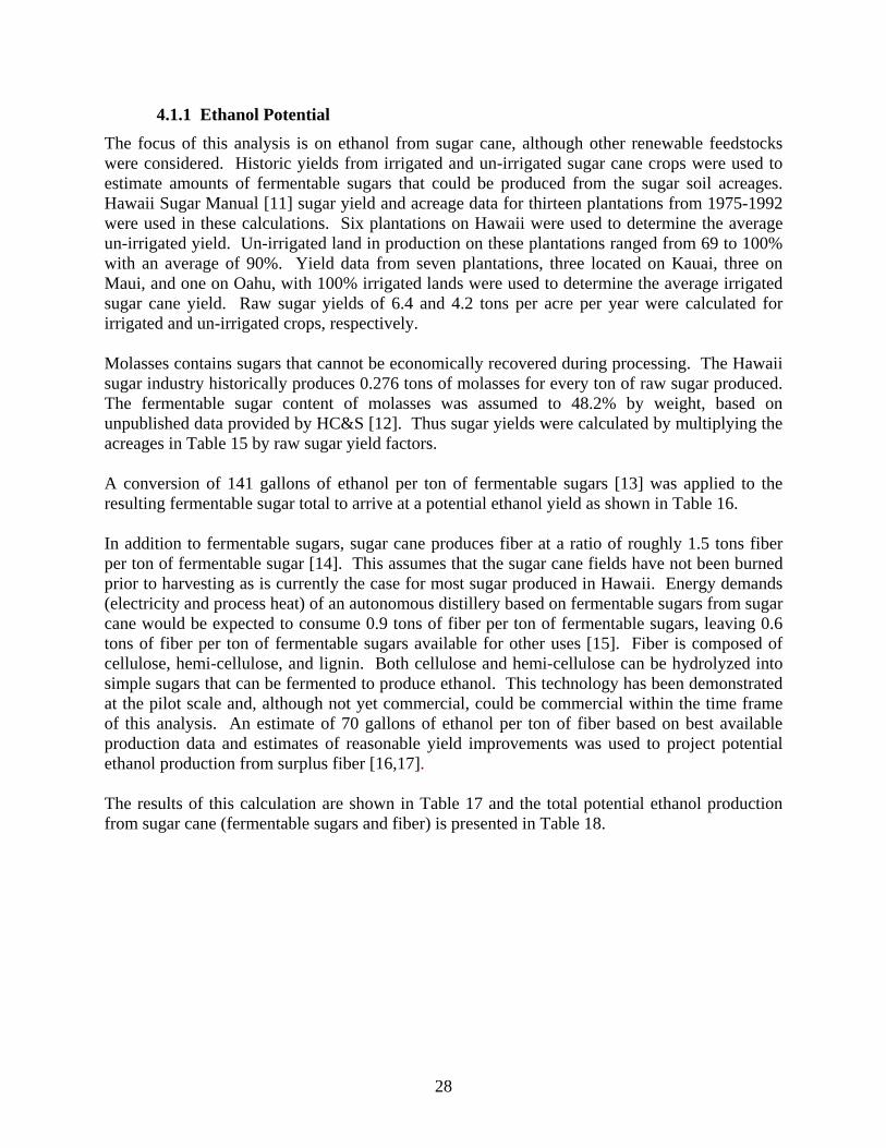
4.1.1 Ethanol Potential The focus of this analysis is on ethanol from sugar cane, although other renewable feedstocks were considered. Historic yields from irrigated and un-irrigated sugar cane crops were used to estimate amounts of fermentable sugars that could be produced from the sugar soil acreages. Hawaii Sugar Manual [11] sugar yield and acreage data for thirteen plantations from 1975-1992 were used in these calculations. Six plantations on Hawaii were used to determine the average un-irrigated yield. Un-irrigated land in production on these plantations ranged from 69 to 100% with an average of 90%. Yield data from seven plantations, three located on Kauai, three on Maui, and one on Oahu, with 100% irrigated lands were used to determine the average irrigated sugar cane yield. Raw sugar yields of 6.4 and 4.2 tons per acre per year were calculated for irrigated and un-irrigated crops, respectively. Molasses contains sugars that cannot be economically recovered during processing. The Hawaii sugar industry historically produces 0.276 tons of molasses for every ton of raw sugar produced. The fermentable sugar content of molasses was assumed to 48.2% by weight, based on unpublished data provided by HC&S [12]. Thus sugar yields were calculated by multiplying the acreages in Table 15 by raw sugar yield factors. A conversion of 141 gallons of ethanol per ton of fermentable sugars [13] was applied to the resulting fermentable sugar total to arrive at a potential ethanol yield as shown in Table 16. In addition to fermentable sugars, sugar cane produces fiber at a ratio of roughly 1.5 tons fiber per ton of fermentable sugar [14]. This assumes that the sugar cane fields have not been burned prior to harvesting as is currently the case for most sugar produced in Hawaii. Energy demands (electricity and process heat) of an autonomous distillery based on fermentable sugars from sugar cane would be expected to consume 0.9 tons of fiber per ton of fermentable sugars, leaving 0.6 tons of fiber per ton of fermentable sugars available for other uses [15]. Fiber is composed of cellulose, hemi-cellulose, and lignin. Both cellulose and hemi-cellulose can be hydrolyzed into simple sugars that can be fermented to produce ethanol. This technology has been demonstrated at the pilot scale and, although not yet commercial, could be commercial within the time frame of this analysis. An estimate of 70 gallons of ethanol per ton of fiber based on best available production data and estimates of reasonable yield improvements was used to project potential ethanol production from surplus fiber [16,17]. The results of this calculation are shown in Table 17 and the total potential ethanol production from sugar cane (fermentable sugars and fiber) is presented in Table 18.

28

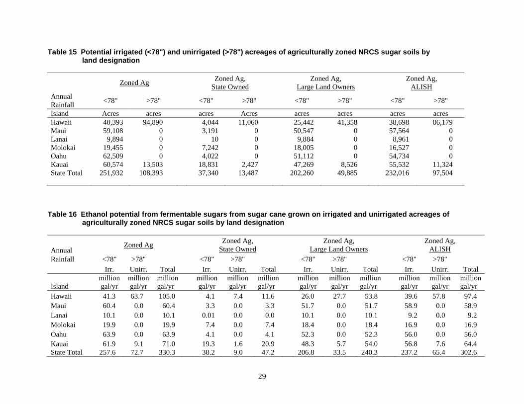
Table 15 Potential irrigated (<78") and unirrigated (>78") acreages of agriculturally zoned NRCS sugar soils by land designation

Zoned Ag, State Owned Zoned Ag,

Large Land Owners Zoned Ag, ALISH Zoned Ag

Annual Rainfall <78" >78" <78" >78" <78" >78" <78" >78"

Island Acres acres acres Acres acres acres acres acres Hawaii 40,393 94,890 4,044 11,060 25,442 41,358 38,698 86,179 Maui 59,108 0 3,191 0 50,547 0 57,564 0 Lanai 9,894 0 10 0 9,884 0 8,961 0 Molokai 19,455 0 7,242 0 18,005 0 16,527 0 Oahu 62,509 0 4,022 0 51,112 0 54,734 0 Kauai 60,574 13,503 18,831 2,427 47,269 8,526 55,532 11,324 State Total 251,932 108,393 37,340 13,487 202,260 49,885 232,016 97,504

Table 16 Ethanol potential from fermentable sugars from sugar cane grown on irrigated and unirrigated acreages of agriculturally zoned NRCS sugar soils by land designation

Zoned Ag, State Owned Zoned Ag,

Large Land Owners Zoned Ag, ALISHAnnual

Zoned Ag

Rainfall <78" >78" <78" >78" <78" >78" <78" >78" Irr. Unirr. Total Irr. Unirr. Total Irr. Unirr. Total Irr. Unirr. Total

Island million gal/yr

million gal/yr

million gal/yr

million gal/yr

million gal/yr

million gal/yr

million gal/yr

million gal/yr

million gal/yr

million gal/yr

million gal/yr

million gal/yr

Hawaii 41.3 63.7 105.0 4.1 7.4 11.6 26.0 27.7 53.8 39.6 57.8 97.4 Maui 60.4 0.0 60.4 3.3 0.0 3.3 51.7 0.0 51.7 58.9 0.0 58.9 Lanai 10.1 0.0 10.1 0.01 0.0 0.0 10.1 0.0 10.1 9.2 0.0 9.2 Molokai 19.9 0.0 19.9 7.4 0.0 7.4 18.4 0.0 18.4 16.9 0.0 16.9 Oahu 63.9 0.0 63.9 4.1 0.0 4.1 52.3 0.0 52.3 56.0 0.0 56.0 Kauai 61.9 9.1 71.0 19.3 1.6 20.9 48.3 5.7 54.0 56.8 7.6 64.4 State Total 257.6 72.7 330.3 38.2 9.0 47.2 206.8 33.5 240.3 237.2 65.4 302.6

29

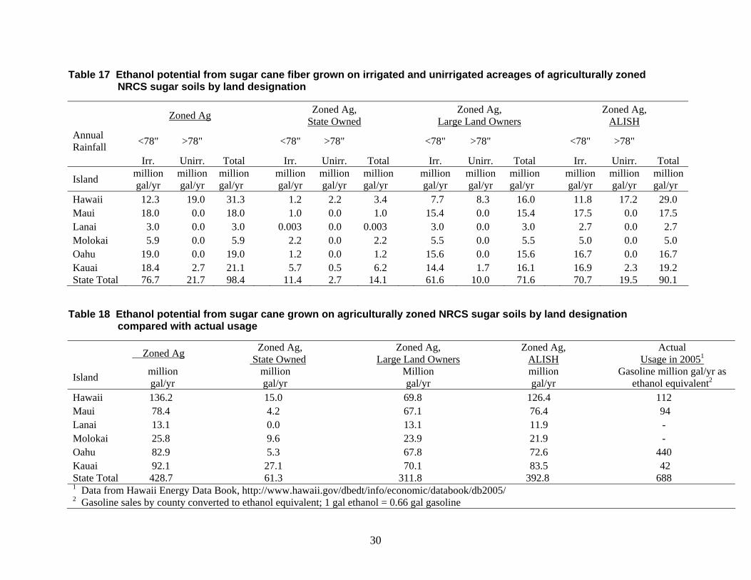
30

Table 17 Ethanol potential from sugar cane fiber grown on irrigated and unirrigated acreages of agriculturally zoned NRCS sugar soils by land designation

Zoned Ag Zoned Ag, State Owned

Zoned Ag, Large Land Owners

Zoned Ag, ALISH

Annual Rainfall <78" >78" <78" >78" <78" >78" <78" >78"

Irr. Unirr. Total Irr. Unirr. Total Irr. Unirr. Total Irr. Unirr. Total

Island million gal/yr

million gal/yr

million gal/yr million

gal/yr million gal/yr

million gal/yr million

gal/yr million gal/yr

million gal/yr million

gal/yr million gal/yr

million gal/yr

Hawaii 12.3 19.0 31.3 1.2 2.2 3.4 7.7 8.3 16.0 11.8 17.2 29.0 Maui 18.0 0.0 18.0 1.0 0.0 1.0 15.4 0.0 15.4 17.5 0.0 17.5 Lanai 3.0 0.0 3.0 0.003 0.0 0.003 3.0 0.0 3.0 2.7 0.0 2.7 Molokai 5.9 0.0 5.9 2.2 0.0 2.2 5.5 0.0 5.5 5.0 0.0 5.0 Oahu 19.0 0.0 19.0 1.2 0.0 1.2 15.6 0.0 15.6 16.7 0.0 16.7 Kauai 18.4 2.7 21.1 5.7 0.5 6.2 14.4 1.7 16.1 16.9 2.3 19.2 State Total 76.7 21.7 98.4 11.4 2.7 14.1 61.6 10.0 71.6 70.7 19.5 90.1

Table 18 Ethanol potential from sugar cane grown on agriculturally zoned NRCS sugar soils by land designation compared with actual usage

Zoned Ag

Zoned Ag, State Owned

Zoned Ag, Large Land Owners

Zoned Ag, ALISH

Actual Usage in 20051

Island million gal/yr million

gal/yr Million gal/yr million

gal/yr Gasoline million gal/yr as ethanol equivalent2

Hawaii 136.2 15.0 69.8 126.4 112 Maui 78.4 4.2 67.1 76.4 94 Lanai 13.1 0.0 13.1 11.9 - Molokai 25.8 9.6 23.9 21.9 - Oahu 82.9 5.3 67.8 72.6 440 Kauai 92.1 27.1 70.1 83.5 42 State Total 428.7 61.3 311.8 392.8 688 1 Data from Hawaii Energy Data Book, http://www.hawaii.gov/dbedt/info/economic/databook/db2005/ 2 Gasoline sales by county converted to ethanol equivalent; 1 gal ethanol = 0.66 gal gasoline

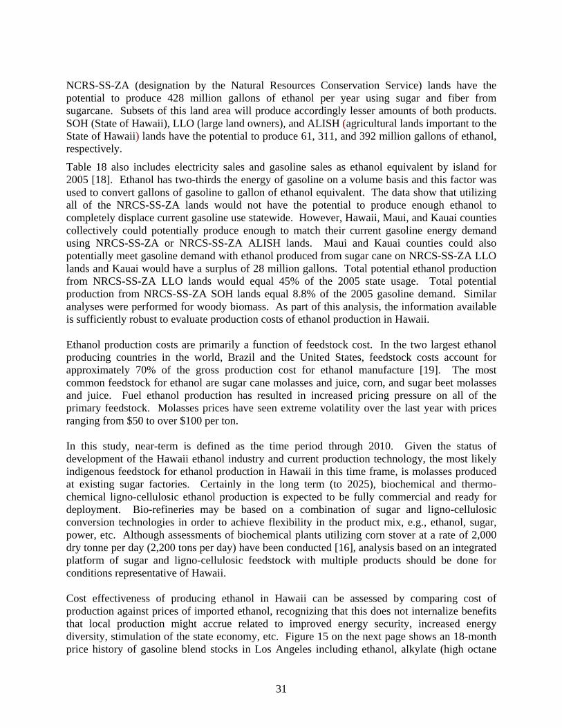
NCRS-SS-ZA (designation by the Natural Resources Conservation Service) lands have the potential to produce 428 million gallons of ethanol per year using sugar and fiber from sugarcane. Subsets of this land area will produce accordingly lesser amounts of both products. SOH (State of Hawaii), LLO (large land owners), and ALISH (agricultural lands important to the State of Hawaii) lands have the potential to produce 61, 311, and 392 million gallons of ethanol, respectively.

Table 18 also includes electricity sales and gasoline sales as ethanol equivalent by island for 2005 [18]. Ethanol has two-thirds the energy of gasoline on a volume basis and this factor was used to convert gallons of gasoline to gallon of ethanol equivalent. The data show that utilizing all of the NRCS-SS-ZA lands would not have the potential to produce enough ethanol to completely displace current gasoline use statewide. However, Hawaii, Maui, and Kauai counties collectively could potentially produce enough to match their current gasoline energy demand using NRCS-SS-ZA or NRCS-SS-ZA ALISH lands. Maui and Kauai counties could also potentially meet gasoline demand with ethanol produced from sugar cane on NRCS-SS-ZA LLO lands and Kauai would have a surplus of 28 million gallons. Total potential ethanol production from NRCS-SS-ZA LLO lands would equal 45% of the 2005 state usage. Total potential production from NRCS-SS-ZA SOH lands equal 8.8% of the 2005 gasoline demand. Similar analyses were performed for woody biomass. As part of this analysis, the information available is sufficiently robust to evaluate production costs of ethanol production in Hawaii. Ethanol production costs are primarily a function of feedstock cost. In the two largest ethanol producing countries in the world, Brazil and the United States, feedstock costs account for approximately 70% of the gross production cost for ethanol manufacture [19]. The most common feedstock for ethanol are sugar cane molasses and juice, corn, and sugar beet molasses and juice. Fuel ethanol production has resulted in increased pricing pressure on all of the primary feedstock. Molasses prices have seen extreme volatility over the last year with prices ranging from $50 to over $100 per ton.

In this study, near-term is defined as the time period through 2010. Given the status of development of the Hawaii ethanol industry and current production technology, the most likely indigenous feedstock for ethanol production in Hawaii in this time frame, is molasses produced at existing sugar factories. Certainly in the long term (to 2025), biochemical and thermo-chemical ligno-cellulosic ethanol production is expected to be fully commercial and ready for deployment. Bio-refineries may be based on a combination of sugar and ligno-cellulosic conversion technologies in order to achieve flexibility in the product mix, e.g., ethanol, sugar, power, etc. Although assessments of biochemical plants utilizing corn stover at a rate of 2,000 dry tonne per day (2,200 tons per day) have been conducted [16], analysis based on an integrated platform of sugar and ligno-cellulosic feedstock with multiple products should be done for conditions representative of Hawaii.

Cost effectiveness of producing ethanol in Hawaii can be assessed by comparing cost of production against prices of imported ethanol, recognizing that this does not internalize benefits that local production might accrue related to improved energy security, increased energy diversity, stimulation of the state economy, etc. Figure 15 on the next page shows an 18-month price history of gasoline blend stocks in Los Angeles including ethanol, alkylate (high octane

31

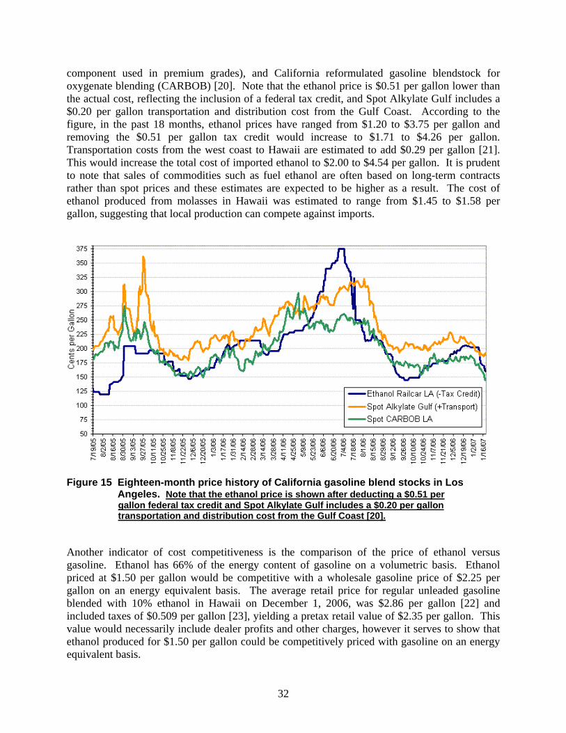
component used in premium grades), and California reformulated gasoline blendstock for oxygenate blending (CARBOB) [20]. Note that the ethanol price is $0.51 per gallon lower than the actual cost, reflecting the inclusion of a federal tax credit, and Spot Alkylate Gulf includes a $0.20 per gallon transportation and distribution cost from the Gulf Coast. According to the figure, in the past 18 months, ethanol prices have ranged from $1.20 to $3.75 per gallon and removing the $0.51 per gallon tax credit would increase to $1.71 to $4.26 per gallon. Transportation costs from the west coast to Hawaii are estimated to add $0.29 per gallon [21]. This would increase the total cost of imported ethanol to $2.00 to $4.54 per gallon. It is prudent to note that sales of commodities such as fuel ethanol are often based on long-term contracts rather than spot prices and these estimates are expected to be higher as a result. The cost of ethanol produced from molasses in Hawaii was estimated to range from $1.45 to $1.58 per gallon, suggesting that local production can compete against imports.

Figure 15 Eighteen-month price history of California gasoline blend stocks in Los Angeles. Note that the ethanol price is shown after deducting a $0.51 per gallon federal tax credit and Spot Alkylate Gulf includes a $0.20 per gallon transportation and distribution cost from the Gulf Coast [20]. Another indicator of cost competitiveness is the comparison of the price of ethanol versus gasoline. Ethanol has 66% of the energy content of gasoline on a volumetric basis. Ethanol priced at $1.50 per gallon would be competitive with a wholesale gasoline price of $2.25 per gallon on an energy equivalent basis. The average retail price for regular unleaded gasoline blended with 10% ethanol in Hawaii on December 1, 2006, was $2.86 per gallon [22] and included taxes of $0.509 per gallon [23], yielding a pretax retail value of $2.35 per gallon. This value would necessarily include dealer profits and other charges, however it serves to show that ethanol produced for $1.50 per gallon could be competitively priced with gasoline on an energy equivalent basis.

32

As part of the complete analysis, sugar cane, banagrass, Leucaena, and Eucalyptus were selected as potential ethanol feedstock crops based on historical crop production in Hawaii or extensive energy crop research trials and demonstrations conducted over the past 30 years. Sugar cane provides fermentable sugars and fiber, whereas the latter three crops are grown for fiber only. Crop water requirements were compared with annual rainfall for the selected land areas. It was assumed that sugar and banagrass would at least require 78 inches of irrigation annually, via rainfall or mechanical application; thus, lands receiving less than 78 inches of rainfall would need some applied irrigation to supplement rainfall. It was assumed that Leucaena and Eucalyptus would be grown without applied irrigation, that Leucaena was suitable for drier locations (20 to 40 inches), and that Eucalyptus was suitable for the areas receiving more than 40 inches of annual rainfall. Historic production data for un-irrigated and irrigated sugar cane in Hawaii were used to calculate average raw sugar yields of 4.2 and 6.4 tons per acre per year, respectively. Based on these values and molasses and fiber data, associated total fermentable sugar and fiber yields were calculated to be 4.6 and 7.1 tons per acre per year for un-irrigated sugar cane and 7.0 and 10.9 tons per acre per year for irrigated sugar cane. Un-irrigated banagrass and irrigated banagrass fiber yields were assumed to be 18 and 22 tons per acre per year, respectively. Fiber yields from Leucaena and Eucalyptus were estimated to be 10 tons per acre per year based on field trials and demonstration plantings. Yields of ethanol from sugar and fiber were assumed to be 141 gallons per ton of fermentable sugars and 70 gallons per ton of fiber, respectively. These were used to calculate total potential statewide ethanol production as shown in Table 19. Four crop scenarios were investigated: 1) sugar cane grown on all soils suitable for sugar, 2) Leucaena and Eucalyptus grown on all soils suitable for trees, 3) sugar cane given first priority, grown on all soils suitable for sugar, and Leucaena and Eucalyptus given second priority, grown on remaining soils suitable for trees, and 4) banagrass grown on all soils suitable for sugar. The third crop scenario produced the most ethanol for each of the land subgroups with a maximum value slightly greater than 700 million gallons of ethanol per year. For comparison, the total motor gasoline sales in Hawaii in 2005 totaled 454 million gallons or 668 million gallons of ethanol on an energy equivalent basis. A renewable fuels target of 20% of motor gasoline, 134 million gallons of ethanol equivalent, could be produced under all crop scenarios with the exception of state owned lands under scenarios 1, 2, and 4. The crop scenarios of the summary table do not reflect near-term potential ethanol production. For the purposes of this study, 2010 production of ethanol from molasses from existing sugar factories using readily available conversion technology was considered near term. Production costs were estimated to be $1.45 to $1.58. Comparison of estimated ethanol import costs based on west coast spot market prices and shipping costs ranged from $2.00 to $4.54 per gallon landed in Hawaii excluding incentives, suggesting that ethanol produced from local feedstock could be cost competitive. Similarly, $1.50 per gallon ethanol from molasses would translate to $2.25 per gallon of gasoline on an energy equivalent basis. Average retail gasoline prices without taxes were

33

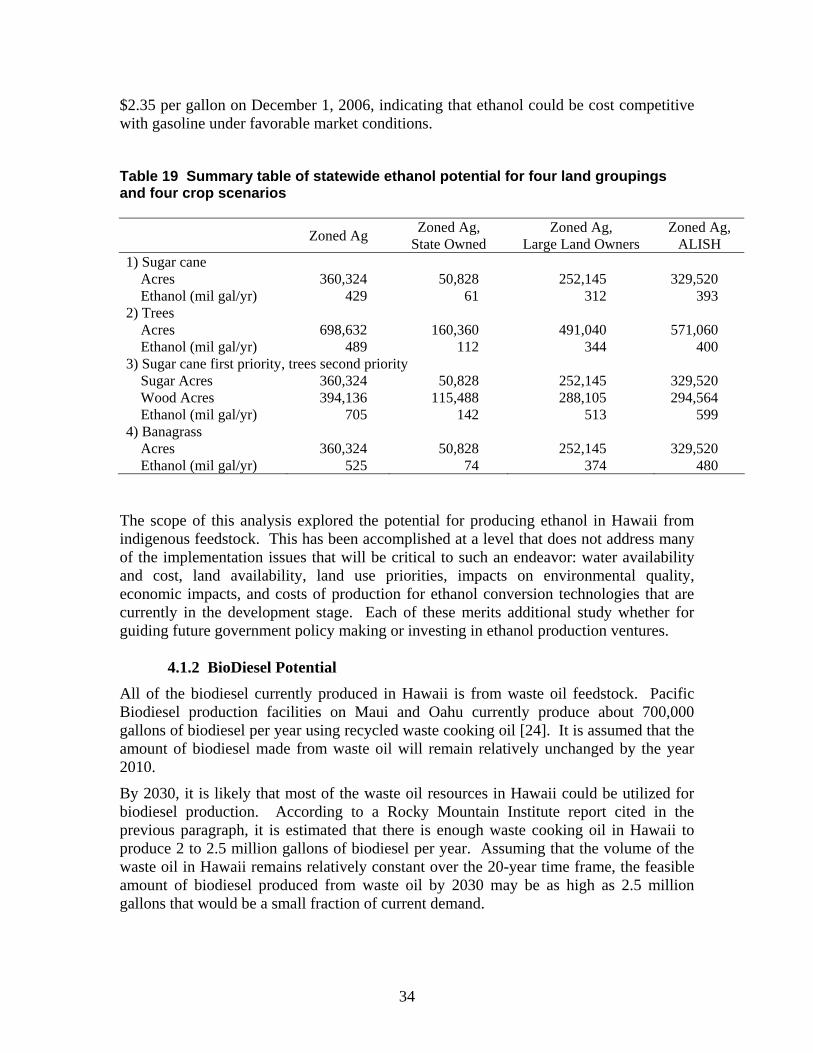
$2.35 per gallon on December 1, 2006, indicating that ethanol could be cost competitive with gasoline under favorable market conditions. Table 19 Summary table of statewide ethanol potential for four land groupings and four crop scenarios

Zoned Ag Zoned Ag, State Owned

Zoned Ag, Large Land Owners

Zoned Ag, ALISH

1) Sugar cane Acres 360,324 50,828 252,145 329,520 Ethanol (mil gal/yr) 429 61 312 393 2) Trees Acres 698,632 160,360 491,040 571,060 Ethanol (mil gal/yr) 489 112 344 400 3) Sugar cane first priority, trees second priority Sugar Acres 360,324 50,828 252,145 329,520 Wood Acres 394,136 115,488 288,105 294,564 Ethanol (mil gal/yr) 705 142 513 599 4) Banagrass Acres 360,324 50,828 252,145 329,520 Ethanol (mil gal/yr) 525 74 374 480

The scope of this analysis explored the potential for producing ethanol in Hawaii from indigenous feedstock. This has been accomplished at a level that does not address many of the implementation issues that will be critical to such an endeavor: water availability and cost, land availability, land use priorities, impacts on environmental quality, economic impacts, and costs of production for ethanol conversion technologies that are currently in the development stage. Each of these merits additional study whether for guiding future government policy making or investing in ethanol production ventures.

4.1.2 BioDiesel Potential

All of the biodiesel currently produced in Hawaii is from waste oil feedstock. Pacific Biodiesel production facilities on Maui and Oahu currently produce about 700,000 gallons of biodiesel per year using recycled waste cooking oil [24]. It is assumed that the amount of biodiesel made from waste oil will remain relatively unchanged by the year 2010.

By 2030, it is likely that most of the waste oil resources in Hawaii could be utilized for biodiesel production. According to a Rocky Mountain Institute report cited in the previous paragraph, it is estimated that there is enough waste cooking oil in Hawaii to produce 2 to 2.5 million gallons of biodiesel per year. Assuming that the volume of the waste oil in Hawaii remains relatively constant over the 20-year time frame, the feasible amount of biodiesel produced from waste oil by 2030 may be as high as 2.5 million gallons that would be a small fraction of current demand.

34

Major growth in the amount of biodiesel produced in Hawaii will only occur with the cultivation of dedicated oil crops or with the importation of agricultural feedstock. A Hawaii Department of Agriculture report prepared by the Hawaii Agriculture Research Center (HARC) examined the potential for oil crop cultivation in Hawaii [25]. The amount of available agricultural land was analyzed on an island by island basis. Factors such as the availability of irrigation water, land slope, and the climatic conditions of the area were taken into account to determine the oil crop best suited for each particular plot of available land.

In total, over 160 million gallons of biodiesel can potentially be produced from oil crops cultivated in Hawaii each year based on the HARC study. This figure is contingent on each island developing its agricultural lands and on the oil crops producing theoretical yields as detailed in the HARC report. None of the crops considered in the study are currently produced on a large agricultural scale in Hawaii, so a number of assumptions were necessary for this quantitative analysis. The potential for feedstock oil production can be altered – sometimes substantially – if any of these assumptions are incorrect. For instance, the area of agricultural land considered available for oil crop cultivation could be reduced if other demands for this resource end up occupying the land. If more of Hawaii’s agricultural lands become available in the future due to a reduction in current agricultural land use, however, the potential for oil production could increase. The oil yields assumed for the crops in the study could be much different when the crops are grown in the Hawaiian climate. Innovative agricultural techniques, such as layering several oil producing species on a plot of land, could increase the oil potential of each acre. Developing appropriate harvesting methods for candidate oil crops will be critical to the technical and economical feasibility of large-scale production. Taking all these factors into account, the annual production of 160 million gallons of oil feedstock potential should be considered a rough estimate. The HARC report does not give an estimate on the time frame needed to implement a statewide agricultural production system capable of supplying 160 million gallons of oil per year. It does state that it will take five to ten years for researchers to determine the best crops and locations for oil production. All of the crops considered in the HARC report take less than ten years to reach production, so it is reasonable to conclude that by 2030, 160 million gallons of oil could be produced per year. It is assumed that there will be no biodiesel production from locally grown oil crops by 2010.

Figure 16 illustrates biodiesel production potential (in 2030) from oil crops for each island as compared to recent petroleum diesel consumption. The total biodiesel production potential is found to be nearly 165 million gallons when the potential for 2.5 million gallons of biodiesel from waste cooking oil is added to the potential for biodiesel production from cultivated oil. If the potential level of biodiesel production is obtained, and if diesel demand remains consistent, Hawaii could be able to replace a reasonable percentage of highway and non-highway diesel used in the state with domestically produced biodiesel.

35

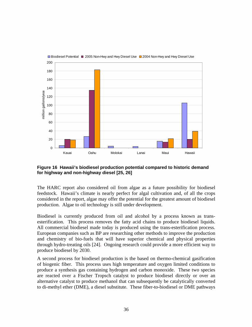
0

20

40

60

80

100

120

140

160

180

200

Kauai Oahu Molokai Lanai Maui Hawaii

mill

ion

gallo

ns/y

ear

Biodiesel Potential 2005 Non-Hwy and Hwy Diesel Use 2004 Non-Hwy and Hwy Diesel Use

Figure 16 Hawaii’s biodiesel production potential compared to historic demand for highway and non-highway diesel [25, 26] The HARC report also considered oil from algae as a future possibility for biodiesel feedstock. Hawaii’s climate is nearly perfect for algal cultivation and, of all the crops considered in the report, algae may offer the potential for the greatest amount of biodiesel production. Algae to oil technology is still under development. Biodiesel is currently produced from oil and alcohol by a process known as trans-esterification. This process removes the fatty acid chains to produce biodiesel liquids. All commercial biodiesel made today is produced using the trans-esterification process. European companies such as BP are researching other methods to improve the production and chemistry of bio-fuels that will have superior chemical and physical properties through hydro-treating oils [24]. Ongoing research could provide a more efficient way to produce biodiesel by 2030.

A second process for biodiesel production is the based on thermo-chemical gasification of biogenic fiber. This process uses high temperature and oxygen limited conditions to produce a synthesis gas containing hydrogen and carbon monoxide. These two species are reacted over a Fischer Tropsch catalyst to produce biodiesel directly or over an alternative catalyst to produce methanol that can subsequently be catalytically converted to di-methyl ether (DME), a diesel substitute. These fiber-to-biodiesel or DME pathways

36

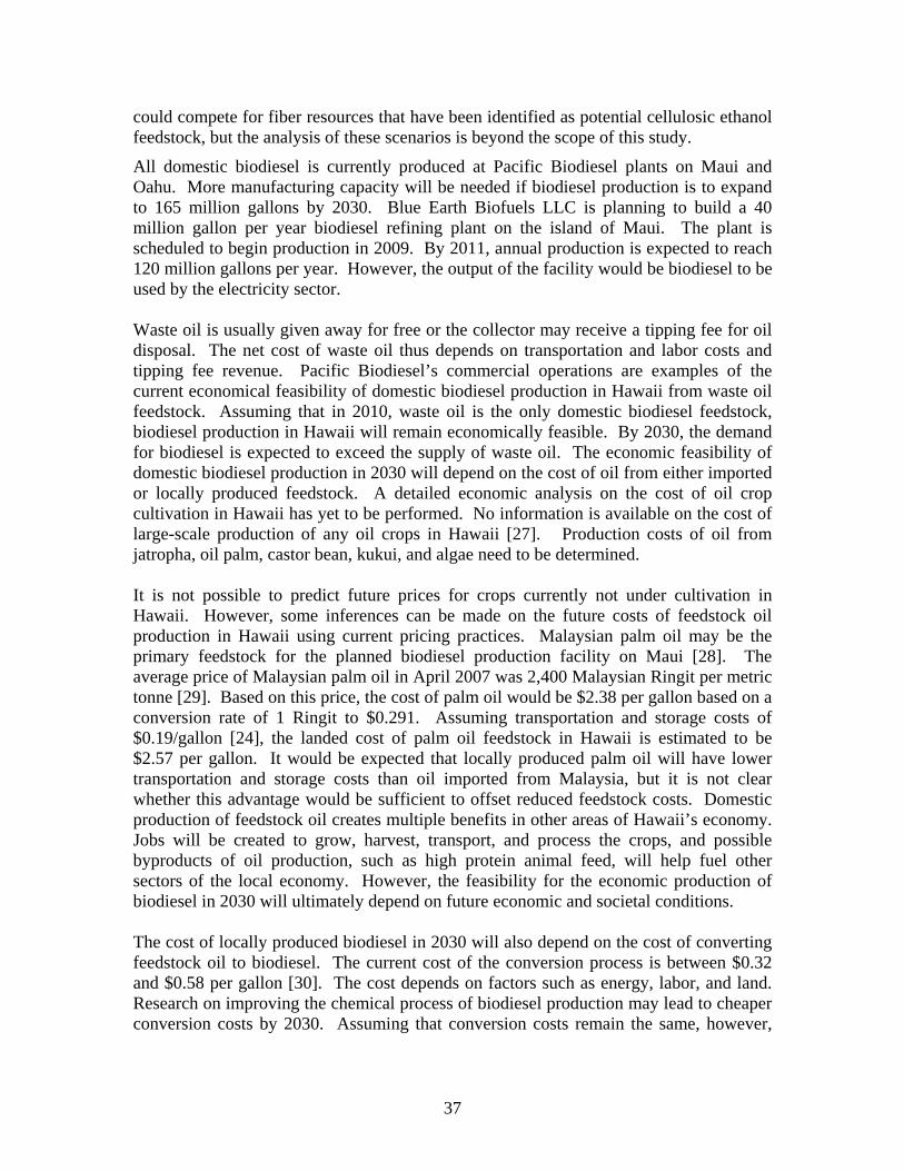
could compete for fiber resources that have been identified as potential cellulosic ethanol feedstock, but the analysis of these scenarios is beyond the scope of this study.

All domestic biodiesel is currently produced at Pacific Biodiesel plants on Maui and Oahu. More manufacturing capacity will be needed if biodiesel production is to expand to 165 million gallons by 2030. Blue Earth Biofuels LLC is planning to build a 40 million gallon per year biodiesel refining plant on the island of Maui. The plant is scheduled to begin production in 2009. By 2011, annual production is expected to reach 120 million gallons per year. However, the output of the facility would be biodiesel to be used by the electricity sector.

Waste oil is usually given away for free or the collector may receive a tipping fee for oil disposal. The net cost of waste oil thus depends on transportation and labor costs and tipping fee revenue. Pacific Biodiesel’s commercial operations are examples of the current economical feasibility of domestic biodiesel production in Hawaii from waste oil feedstock. Assuming that in 2010, waste oil is the only domestic biodiesel feedstock, biodiesel production in Hawaii will remain economically feasible. By 2030, the demand for biodiesel is expected to exceed the supply of waste oil. The economic feasibility of domestic biodiesel production in 2030 will depend on the cost of oil from either imported or locally produced feedstock. A detailed economic analysis on the cost of oil crop cultivation in Hawaii has yet to be performed. No information is available on the cost of large-scale production of any oil crops in Hawaii [27]. Production costs of oil from jatropha, oil palm, castor bean, kukui, and algae need to be determined.

It is not possible to predict future prices for crops currently not under cultivation in Hawaii. However, some inferences can be made on the future costs of feedstock oil production in Hawaii using current pricing practices. Malaysian palm oil may be the primary feedstock for the planned biodiesel production facility on Maui [28]. The average price of Malaysian palm oil in April 2007 was 2,400 Malaysian Ringit per metric tonne [29]. Based on this price, the cost of palm oil would be $2.38 per gallon based on a conversion rate of 1 Ringit to $0.291. Assuming transportation and storage costs of $0.19/gallon [24], the landed cost of palm oil feedstock in Hawaii is estimated to be $2.57 per gallon. It would be expected that locally produced palm oil will have lower transportation and storage costs than oil imported from Malaysia, but it is not clear whether this advantage would be sufficient to offset reduced feedstock costs. Domestic production of feedstock oil creates multiple benefits in other areas of Hawaii’s economy. Jobs will be created to grow, harvest, transport, and process the crops, and possible byproducts of oil production, such as high protein animal feed, will help fuel other sectors of the local economy. However, the feasibility for the economic production of biodiesel in 2030 will ultimately depend on future economic and societal conditions.

The cost of locally produced biodiesel in 2030 will also depend on the cost of converting feedstock oil to biodiesel. The current cost of the conversion process is between $0.32 and $0.58 per gallon [30]. The cost depends on factors such as energy, labor, and land. Research on improving the chemical process of biodiesel production may lead to cheaper conversion costs by 2030. Assuming that conversion costs remain the same, however,

37

and assuming a local feedstock cost of $2.57 per gallon (import parity), the price of locally produced biodiesel in 2030 is projected to be between $2.89 and $3.15 per gallon.

The economic analysis of local biodiesel manufacturing should take into account the economic benefits of its production. Construction costs for the planned biodiesel manufacturing plant on Maui are expected to total $61 million dollars [28]. The construction of the refinery is expected to employ 100 workers and will also provide 40 permanent jobs upon reaching full operating capacity [31].

To conclude, the technical and economic feasibilities for domestic biodiesel production in Hawaii were evaluated and found to depend on the volume of feedstock oil, the biodiesel production technologies, and the availability of manufacturing facilities. The domestic biodiesel production potential in 2010 was found to remain the same as current levels, which is about 700,000 gallons per year. The estimated production assumes the use of current biodiesel manufacturing technology and facilities and use of recycled waste oil as feedstock.

By 2030, biodiesel production from recycled waste oil and cultivated oil feedstock was projected to have statewide production potential of 165 million gallons annually. This estimate depends on specific oil crop cultivation on seven Hawaiian Islands. The 2030 biodiesel potential could be increased if higher yielding oil crops were developed and if more agricultural land becomes available. Large biodiesel production facilities will be needed to create this volume of fuel.

The economic feasibility of domestic biodiesel depends on the costs of production. By 2030 larger-scale domestic biodiesel production will depend on oil crop production. With feedstock costs accounting for more than 60% of biodiesel production costs, the economic feasibility of biodiesel production is heavily dependent on competitively produced oil crops. Domestic oil production will only be feasible if the costs are competitive with global prices of feedstock oil. Since the current price of imported Malaysian palm oil is $2.57 per gallon, domestic crop oil should target a similar price. If feedstock is available for $2.57 per gallon, locally produced biodiesel will cost between $2.89 and $3.15 per gallon. The multiplication of economic benefits associated with domestic oil crop and biodiesel production should also be considered as part of the analysis.

4.1.3 Summary Statement: Transportation Fuels from Renewable Resources

To conclude this analysis of the potential for accelerated renewable resources for transportation fuels, there is clear potential in the state to develop indigenous resources that could be used to replace petroleum products. However, the feasibility depends upon factors that are exogenous to each individual fuel cycle. From an agricultural perspective, land use, water availability, and available labor significant issues need to be addressed. Public opinion concerning the use of land for fuel instead of food is not to be dismissed. For all of the analyses contained in this section, there has been no attempt to address the nature of the competition for resources between ethanol and biodiesel production. Finally, there needs to be a clear linkage between agriculture, production facilities, and end use. These are practical economic and business issues that have not been addressed here.

38

4.2 Renewable Power Options for Electricity Generation

This section addresses another scenario required under Section 355, specifically the evaluation of accelerated use of renewable resources for electricity generation. This section is a summary of a larger report produced as part of the 355 program by P. Lilienthal et al. Three important caveats are important to consider at the beginning of this section. First, similar to the previous section, no attempt has been made to assess competition for resources between renewable resources derived from agriculture. Second, although discussed in the following analysis, it should be emphasized that no attempt has been made to address grid stability and frequency problems associated with a significant percentage of intermittent renewable energy systems deployed on a grid.

Finally, due to funding issues early in the project, the lead for this effort, the National Renewable Energy Laboratory (NREL), was unable to complete the entire analysis in the time required under this contract. It is noted here that DBEDT was notified of this fact when it became apparent that not all of the analyses could be completed on time. Thus, the focus of the early part of the work was to evaluate the ability of the NREL model, HOMER, to be used in the broader analysis. Therefore, an intensive evaluation was performed on one island, Molokai, to assess the model’s efficacy for the rest of the study. NREL has now been funded to complete the remainder of the study by the Department of Energy under a separate contract.

NREL worked with Maui Electric Company to gather data necessary to run an initial test case for the island of Molokai. The resulting analysis shows that increasing levels of wind power could be very cost-effective. It is estimated that diesel fuel use could be reduced from 38% to 70% with overall life cycle cost savings between 20% and 40%. Other renewable energy technologies, such as flat-plate photovoltaic systems and biomass were not found to be as economic as wind or diesel power.

The analysis for Molokai also highlighted some areas requiring additional analysis needed before implementing high penetrations of renewable energy. This is because there is an awareness of grid stability issues associated with wind variability and intermittency on other islands in the state. Thus, results would depend on how the utility handles integration issues, such as spinning reserves, advanced generation controls, and operations and maintenance issues associated with running diesel generators at lower load levels. It should be pointed out that this analysis did not attempt to treat the Molokai grid as part of the larger Maui electric company system. Rather, this was examined as a stand-alone system.

Several cases were run to test the sensitivity of the results to several variables. Some of these variables are uncertain, while others would be embedded in decisions that MECO must make over how to dispatch the diesel generators within their system, which can have a substantial effect on the integration of wind power into the system. As shown in Figure 17 on the next page, the optimal number of 1.5-MW turbines varies from three to six and the resulting fuel consumption varies from 3,480,000 liters to 7,211,000 liters.

39

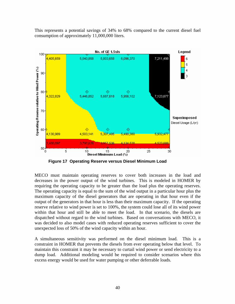
This represents a potential savings of 34% to 68% compared to the current diesel fuel consumption of approximately 11,000,000 liters.

Figure 17 Operating Reserve versus Diesel Minimum Load

MECO must maintain operating reserves to cover both increases in the load and decreases in the power output of the wind turbines. This is modeled in HOMER by requiring the operating capacity to be greater than the load plus the operating reserves. The operating capacity is equal to the sum of the wind output in a particular hour plus the maximum capacity of the diesel generators that are operating in that hour even if the output of the generators in that hour is less than their maximum capacity. If the operating reserve relative to wind power is set to 100%, the system could lose all of its wind power within that hour and still be able to meet the load. In that scenario, the diesels are dispatched without regard to the wind turbines. Based on conversations with MECO, it was decided to also model cases with reduced operating reserves sufficient to cover the unexpected loss of 50% of the wind capacity within an hour. A simultaneous sensitivity was performed on the diesel minimum load. This is a constraint in HOMER that prevents the diesels from ever operating below that level. To maintain this constraint it may be necessary to curtail wind power or send electricity to a dump load. Additional modeling would be required to consider scenarios where this excess energy would be used for water pumping or other deferrable loads.

40

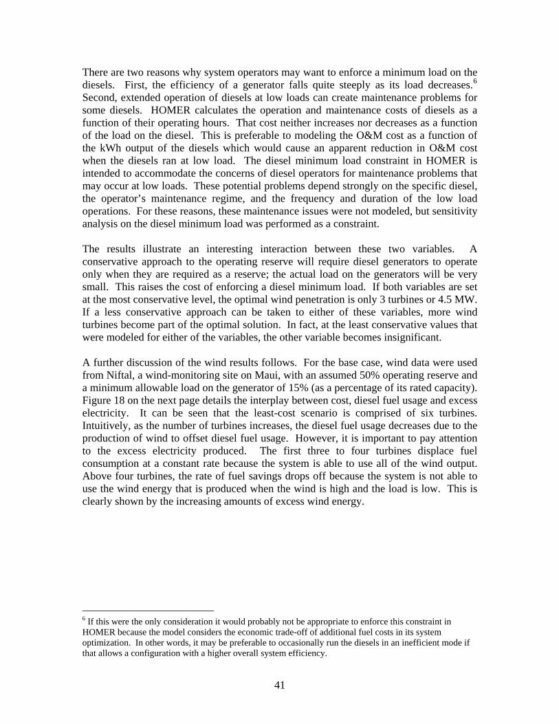
There are two reasons why system operators may want to enforce a minimum load on the diesels. First, the efficiency of a generator falls quite steeply as its load decreases.6 Second, extended operation of diesels at low loads can create maintenance problems for some diesels. HOMER calculates the operation and maintenance costs of diesels as a function of their operating hours. That cost neither increases nor decreases as a function of the load on the diesel. This is preferable to modeling the O&M cost as a function of the kWh output of the diesels which would cause an apparent reduction in O&M cost when the diesels ran at low load. The diesel minimum load constraint in HOMER is intended to accommodate the concerns of diesel operators for maintenance problems that may occur at low loads. These potential problems depend strongly on the specific diesel, the operator’s maintenance regime, and the frequency and duration of the low load operations. For these reasons, these maintenance issues were not modeled, but sensitivity analysis on the diesel minimum load was performed as a constraint. The results illustrate an interesting interaction between these two variables. A conservative approach to the operating reserve will require diesel generators to operate only when they are required as a reserve; the actual load on the generators will be very small. This raises the cost of enforcing a diesel minimum load. If both variables are set at the most conservative level, the optimal wind penetration is only 3 turbines or 4.5 MW. If a less conservative approach can be taken to either of these variables, more wind turbines become part of the optimal solution. In fact, at the least conservative values that were modeled for either of the variables, the other variable becomes insignificant.

A further discussion of the wind results follows. For the base case, wind data were used from Niftal, a wind-monitoring site on Maui, with an assumed 50% operating reserve and a minimum allowable load on the generator of 15% (as a percentage of its rated capacity). Figure 18 on the next page details the interplay between cost, diesel fuel usage and excess electricity. It can be seen that the least-cost scenario is comprised of six turbines. Intuitively, as the number of turbines increases, the diesel fuel usage decreases due to the production of wind to offset diesel fuel usage. However, it is important to pay attention to the excess electricity produced. The first three to four turbines displace fuel consumption at a constant rate because the system is able to use all of the wind output. Above four turbines, the rate of fuel savings drops off because the system is not able to use the wind energy that is produced when the wind is high and the load is low. This is clearly shown by the increasing amounts of excess wind energy.

6 If this were the only consideration it would probably not be appropriate to enforce this constraint in HOMER because the model considers the economic trade-off of additional fuel costs in its system optimization. In other words, it may be preferable to occasionally run the diesels in an inefficient mode if that allows a configuration with a higher overall system efficiency.

41

Figure 18 Molokai 50% Operating Reserve, 15% Min Load, $0.35/Liter Fuel Price

Million ($, Liters, kWh)

60 50 40 30 20 10 0

0 2 3 1 4 5 6 7 8 9

# of GE 1.5 MW Turbines

Net Present Cost(Million $)Diesel Fuel Usage(Million Liters)Excess Electricity(Million kWh)

A sensitivity analysis was also performed using Puunene wind data, which is the lowest wind resource of the nine Hawaii sites. This analysis was done to examine the effect of a lower wind resource on the feasibility of wind turbines on Molokai. The results show that wind turbine deployment on Molokai is still cost effective. However, the least-cost system comprises four turbines and uses almost 7.5 million liters of fuel when a weaker wind resource is available. Thus, even if Molokai has a weaker wind resource than assumed in the base-case scenario, wind is still cost effective, but on a smaller scale. In addition to identifying the least-cost system, HOMER can also perform a constrained optimization. This constrained optimization was used to identify the least-cost approach to achieving additional diesel fuel savings. In order to achieve greater fuel savings, the use of large-scale vanadium redox flow batteries was considered. It should be noted that this analysis could also be performed using other energy storage systems, such as sodium-sulfur systems. The results in the following graph refer only to the busbar cost of electricity and do not include distribution or administrative costs. In the base-case analysis, the lowest cost system contained six turbines and no storage and consumed approximately 4,000,000 liters of fuel.

Preliminary analysis was performed on the cost-effectiveness of photovoltaic (PV) systems. A sensitivity analysis was performed in HOMER that illustrated that PV was not part of the optimal solution until its capital cost was less than $1.50 per watt, including inverter and installation costs. The exceptionally good wind resource reduces the comparative cost-effectiveness of PV. When all of the cost-effective wind is installed, there are substantial periods of time when excess energy is available. During these periods, any power produced by PV would not be usable. These results could change with the use of more load management or storage and could be examined further in a more detailed analysis.

42

There is considerable opportunity for load management on Molokai. In particular, there is a substantial water pumping load which is currently being managed by pumping at night. This is an appropriate load-management practice for the current system and is partly responsible for the high load factor of the Molokai system. A more detailed analysis should be performed to identify ways to modify this strategy under a scenario with a high level of wind penetration. The analysis in this section has demonstrated that the NREL HOMER approach can be used to evaluate the potential for renewable energy systems for electricity generation on other islands. That work is now proceeding. However, for the purposes of this report, not enough data are available to allow for an evaluation of widespread displacement of oil-fired generation with renewable resources. This is because the electricity system on Molokai is substantively different from that of the major islands. So, it is unclear how much of these results would transfer to these other islands. Specifically the level of wind penetration could be much lower, since Molokai has the advantage of diesel generators that can ramp up and down very quickly. For these reasons, no information from this part of the study was used for additional analyses.

4.3 Liquefied Natural Gas (LNG)

There has been considerable interest in the development of infrastructure to add natural gas to the mix of energy resources for the state of Hawaii. Much of this must remain speculative at the moment, since sources of supply and issues associated with critical infrastructure protection remain to be resolved. However, the analysis provided information and conclusions to suggest that, with the right kind of public incentives and private sector contracts, LNG or compressed natural gas (CNG) could provide another economic energy resource to the state. This study, entitled “Evaluating Natural Gas Import Options for the State of Hawaii” by FACTS Global Research [5] is summarized in this section.

There are a number of possible demand scenarios for LNG for the state. As reflected in Figure 19 on the next page, electricity generation would likely dominate LNG use. According to the studies estimates, if all of the major oil fired power plants on Oahu were to be converted to gas, Hawaii would require approximately 1.40 million tonnes (mt) of LNG in 2013 (a hypothetical date for first imports) for use in power generation. This would grow to 1.48 mt by 2020. In comparison to consumption in the power sector, the Oahu utility gas market is likely to be quite small (an estimated 0.067 mt in 2013). However, there is considerable room for growth as the price of utility gas may be reduced with LNG imports. Over time, there is the possibility that other uses may emerge, including CNG for vehicles, neighbor island use, and reforming natural gas into hydrogen for fuel cells.

43

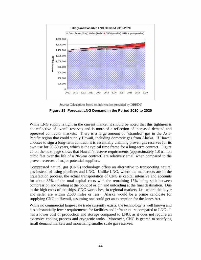
Likely and Possible LNG Demand 2010-2020

0

200,000

400,000

600,000

800,000

1,000,000

1,200,000

1,400,000

1,600,000

1,800,000

2010 2011 2012 2013 2014 2015 2016 2017 2018 2019 2020

Tonn

es o

f LN

G

Oahu Power (likely) Gas (likely) CNG (possible) Hydrogen (possible)

Source: Calculations based on information provided by DBEDT

Figure 19 Forecast LNG Demand in the Period 2010 to 2020 While LNG supply is tight in the current market, it should be noted that this tightness is not reflective of overall reserves and is more of a reflection of increased demand and squeezed contractor markets. There is a large amount of “stranded” gas in the Asia-Pacific region that could supply Hawaii, including domestic gas from Alaska. If Hawaii chooses to sign a long-term contract, it is essentially claiming proven gas reserves for its own use for 20-30 years, which is the typical time frame for a long-term contract. Figure 20 on the next page shows that Hawaii’s reserve requirements (approximately 1.8 trillion cubic feet over the life of a 20-year contract) are relatively small when compared to the proven reserves of major potential suppliers.

Compressed natural gas (CNG) technology offers an alternative to transporting natural gas instead of using pipelines and LNG. Unlike LNG, where the main costs are in the liquefaction process, the actual transportation of CNG is capital intensive and accounts for about 85% of the total capital costs with the remaining 15% being split between compression and loading at the point of origin and unloading at the final destination. Due to the high costs of the ships, CNG works best in regional markets, i.e., where the buyer and seller are within 2,500 miles or less. Alaska would be a prime candidate for supplying CNG to Hawaii, assuming one could get an exemption for the Jones Act.

While no commercial large-scale trade currently exists, the technology is well known and has substantially fewer requirements for facilities and infrastructure compared to LNG. It has a lower cost of production and storage compared to LNG, as it does not require an extensive cooling process and cryogenic tanks. Moreover, CNG is geared to satisfying small demand markets and monetizing smaller scale gas reserves.

44

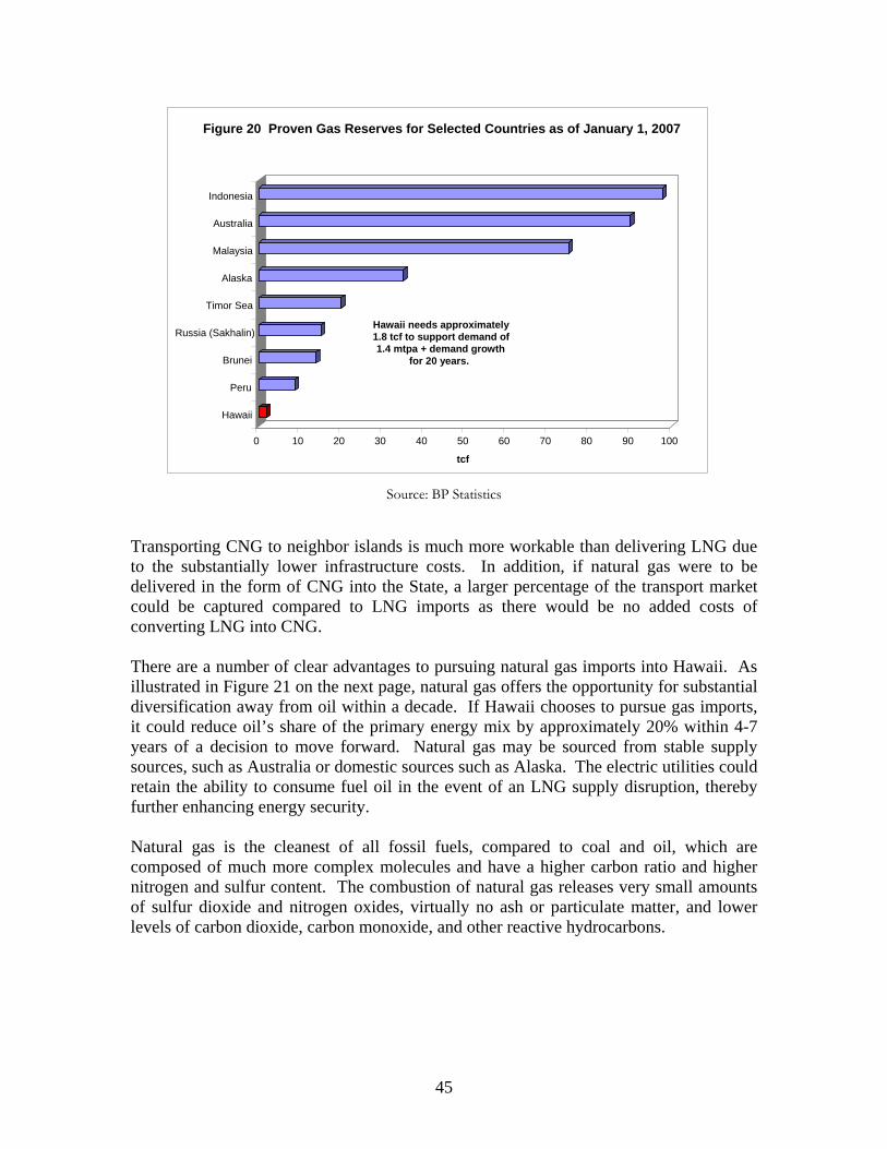
0 10 20 30 40 50 60 70 80 90 100

tcf

Hawaii Peru

Brunei

Russia (Sakhalin)

Timor Sea

Alaska

Malaysia Australia

Indonesia

Figure 20 Proven Gas Reserves for Selected Countries as of January 1, 2007

Hawaii needs approximately 1.8 tcf to support demand of 1.4 mtpa + demand growth

for 20 years.

Source: BP Statistics

Transporting CNG to neighbor islands is much more workable than delivering LNG due to the substantially lower infrastructure costs. In addition, if natural gas were to be delivered in the form of CNG into the State, a larger percentage of the transport market could be captured compared to LNG imports as there would be no added costs of converting LNG into CNG. There are a number of clear advantages to pursuing natural gas imports into Hawaii. As illustrated in Figure 21 on the next page, natural gas offers the opportunity for substantial diversification away from oil within a decade. If Hawaii chooses to pursue gas imports, it could reduce oil’s share of the primary energy mix by approximately 20% within 4-7 years of a decision to move forward. Natural gas may be sourced from stable supply sources, such as Australia or domestic sources such as Alaska. The electric utilities could retain the ability to consume fuel oil in the event of an LNG supply disruption, thereby further enhancing energy security. Natural gas is the cleanest of all fossil fuels, compared to coal and oil, which are composed of much more complex molecules and have a higher carbon ratio and higher nitrogen and sulfur content. The combustion of natural gas releases very small amounts of sulfur dioxide and nitrogen oxides, virtually no ash or particulate matter, and lower levels of carbon dioxide, carbon monoxide, and other reactive hydrocarbons.

45

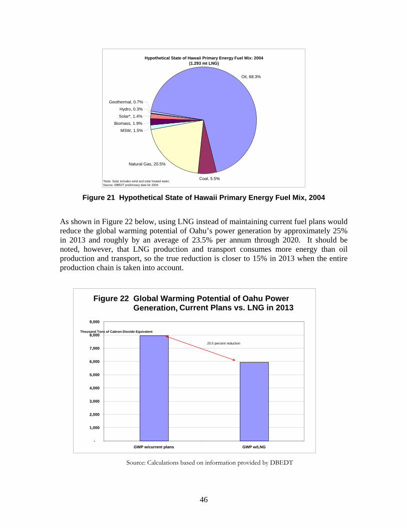
Hypothetical State of Hawaii Primary Energy Fuel Mix: 2004(1.293 mt LNG)

Oil, 68.3%

Coal, 5.5%

Natural Gas, 20.5%

MSW, 1.5%

Biomass, 1.9%

Solar*, 1.4%

Hydro, 0.3%

Geothermal, 0.7%

*Note: Solar includes wind and solar heated water.Source: DBEDT preliminary data for 2004.

Figure 21 Hypothetical State of Hawaii Primary Energy Fuel Mix, 2004 As shown in Figure 22 below, using LNG instead of maintaining current fuel plans would reduce the global warming potential of Oahu’s power generation by approximately 25% in 2013 and roughly by an average of 23.5% per annum through 2020. It should be noted, however, that LNG production and transport consumes more energy than oil production and transport, so the true reduction is closer to 15% in 2013 when the entire production chain is taken into account.

Figure 22 Global Warming Potential of Oahu Power Generation, Current Plans vs. LNG in 2013

-

1,000

2,000

3,000

4,000

5,000

6,000

7,000

8,000

9,000

GWP w/current plans GWP w/LNG

Thousand Tons of Cabron-Dioxide Equivalent 25.5 percent reduction

Source: Calculations based on information provided by DBEDT

46

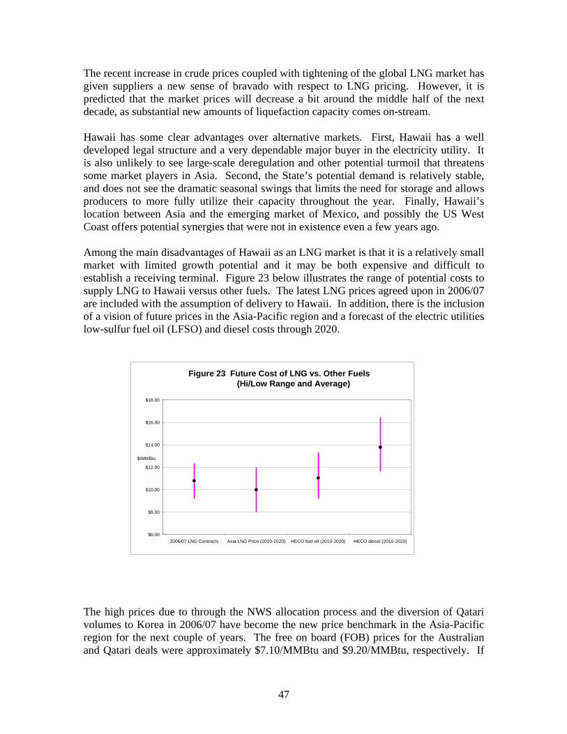
The recent increase in crude prices coupled with tightening of the global LNG market has given suppliers a new sense of bravado with respect to LNG pricing. However, it is predicted that the market prices will decrease a bit around the middle half of the next decade, as substantial new amounts of liquefaction capacity comes on-stream. Hawaii has some clear advantages over alternative markets. First, Hawaii has a well developed legal structure and a very dependable major buyer in the electricity utility. It is also unlikely to see large-scale deregulation and other potential turmoil that threatens some market players in Asia. Second, the State’s potential demand is relatively stable, and does not see the dramatic seasonal swings that limits the need for storage and allows producers to more fully utilize their capacity throughout the year. Finally, Hawaii’s location between Asia and the emerging market of Mexico, and possibly the US West Coast offers potential synergies that were not in existence even a few years ago. Among the main disadvantages of Hawaii as an LNG market is that it is a relatively small market with limited growth potential and it may be both expensive and difficult to establish a receiving terminal. Figure 23 below illustrates the range of potential costs to supply LNG to Hawaii versus other fuels. The latest LNG prices agreed upon in 2006/07 are included with the assumption of delivery to Hawaii. In addition, there is the inclusion of a vision of future prices in the Asia-Pacific region and a forecast of the electric utilities low-sulfur fuel oil (LFSO) and diesel costs through 2020.

Figure 23 Future Cost of LNG vs. Other Fuels(Hi/Low Range and Average)

$6.00

$8.00

$10.00

$12.00

$14.00

$16.00

$18.00

2006/07 LNG Contracts Asia LNG Price (2010-2020) HECO fuel oil (2010-2020) HECO diesel (2010-2020)

$/MMBtu

The high prices due to through the NWS allocation process and the diversion of Qatari volumes to Korea in 2006/07 have become the new price benchmark in the Asia-Pacific region for the next couple of years. The free on board (FOB) prices for the Australian and Qatari deals were approximately $7.10/MMBtu and $9.20/MMBtu, respectively. If

47

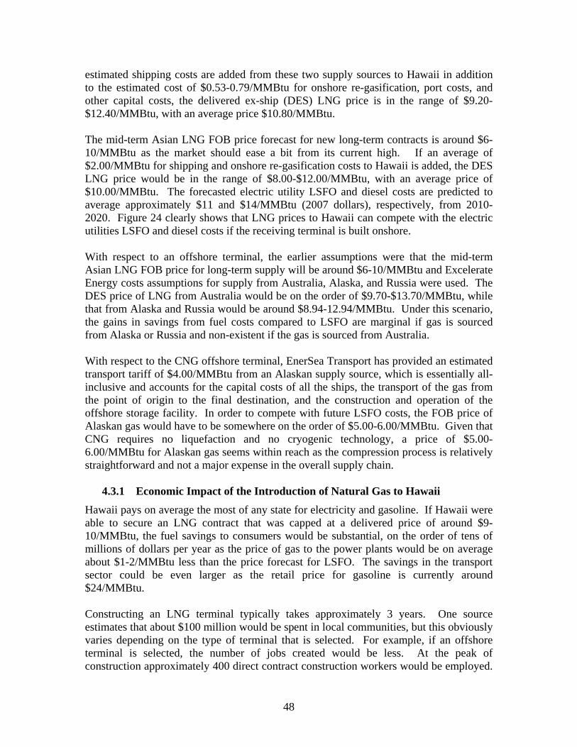
estimated shipping costs are added from these two supply sources to Hawaii in addition to the estimated cost of $0.53-0.79/MMBtu for onshore re-gasification, port costs, and other capital costs, the delivered ex-ship (DES) LNG price is in the range of $9.20-$12.40/MMBtu, with an average price $10.80/MMBtu. The mid-term Asian LNG FOB price forecast for new long-term contracts is around $6-10/MMBtu as the market should ease a bit from its current high. If an average of $2.00/MMBtu for shipping and onshore re-gasification costs to Hawaii is added, the DES LNG price would be in the range of $8.00-$12.00/MMBtu, with an average price of $10.00/MMBtu. The forecasted electric utility LSFO and diesel costs are predicted to average approximately $11 and $14/MMBtu (2007 dollars), respectively, from 2010-2020. Figure 24 clearly shows that LNG prices to Hawaii can compete with the electric utilities LSFO and diesel costs if the receiving terminal is built onshore. With respect to an offshore terminal, the earlier assumptions were that the mid-term Asian LNG FOB price for long-term supply will be around $6-10/MMBtu and Excelerate Energy costs assumptions for supply from Australia, Alaska, and Russia were used. The DES price of LNG from Australia would be on the order of $9.70-$13.70/MMBtu, while that from Alaska and Russia would be around $8.94-12.94/MMBtu. Under this scenario, the gains in savings from fuel costs compared to LSFO are marginal if gas is sourced from Alaska or Russia and non-existent if the gas is sourced from Australia.

With respect to the CNG offshore terminal, EnerSea Transport has provided an estimated transport tariff of $4.00/MMBtu from an Alaskan supply source, which is essentially all-inclusive and accounts for the capital costs of all the ships, the transport of the gas from the point of origin to the final destination, and the construction and operation of the offshore storage facility. In order to compete with future LSFO costs, the FOB price of Alaskan gas would have to be somewhere on the order of $5.00-6.00/MMBtu. Given that CNG requires no liquefaction and no cryogenic technology, a price of $5.00-6.00/MMBtu for Alaskan gas seems within reach as the compression process is relatively straightforward and not a major expense in the overall supply chain.

4.3.1 Economic Impact of the Introduction of Natural Gas to Hawaii

Hawaii pays on average the most of any state for electricity and gasoline. If Hawaii were able to secure an LNG contract that was capped at a delivered price of around $9-10/MMBtu, the fuel savings to consumers would be substantial, on the order of tens of millions of dollars per year as the price of gas to the power plants would be on average about $1-2/MMBtu less than the price forecast for LSFO. The savings in the transport sector could be even larger as the retail price for gasoline is currently around $24/MMBtu. Constructing an LNG terminal typically takes approximately 3 years. One source estimates that about $100 million would be spent in local communities, but this obviously varies depending on the type of terminal that is selected. For example, if an offshore terminal is selected, the number of jobs created would be less. At the peak of construction approximately 400 direct contract construction workers would be employed.

48

If all direct, indirect, and induced jobs (i.e., the employment multiplier) are included, almost 900 jobs could be created over the course of the construction period. An LNG terminal would have approximately 45 direct full-time employees once it is in operation. Because it is not an established industry in the state, it is not clear what the employment multiplier is for LNG, but if the employment multiplier for the power industry (3.10) and the job multiplier for the petroleum industry (4.63) are taken as guidelines, between 140 and 208 jobs would be created in the overall economy.7 With respect to investment, end-use activities are likely the best area in the chain for locally-based investment opportunities. The primary sectors for end-use are power, industrial, residential/commercial, and transportation. Investment in the transport sector is the most intriguing as there will be a need for businesses that can be contracted to convert vehicles and to maintain and service vehicles running on natural gas. Such businesses will also need to cover refueling, which means increasing the number of service stations or piggybacking on existing ones.

4.3.2 The Hydrogen Option

Title 8 of the 2005 Energy Policy Act coupled with the Advanced Energy Initiative and the President’s Hydrogen Fuel Initiative has helped to reduce many of the costs associated with hydrogen production, though substantial cost reductions are still necessary for hydrogen to be cost competitive with existing fuel sources. Hawaii is arguably among the best sites in the US to explore this technology – electricity generated via geothermal, solar, and wind power has long been viewed as the ideal, albeit currently expensive, emissions-free means of producing hydrogen for fuel cells (via electrolysis of water). In spite of its promise, the high cost of producing hydrogen and developing a hydrogen infrastructure is a considerable roadblock along the path towards an emissions-free hydrogen economy. There is, however, a possible solution in bridging the gap towards a Hawaii hydrogen economy – natural gas. Natural gas is currently the least expensive feedstock for producing hydrogen (see Figure 24 on the next page). However, it should be pointed out that natural gas is not viewed as a viable long-term feedstock for hydrogen production because it is not emissions free, it is not a renewable resource, its price is volatile, and there are competing demands for supply in other sectors (power, residential, commercial, and industrial). Eventually, the hope would be to move away from a dependence on natural gas and to produce hydrogen using electricity that is generated from renewable sources. It was beyond the funding level for this overall study to properly analyze the potential for hydrogen production and use for the state of Hawaii.

7 Source: Eugene Tian, DBEDT

49

Dollars/Gallon of Gasoline Equivalent

10

9

8

7

6

5

4

3

2

1

0Natural Gas Biomass

GasificationCoal

GasificationDistributed

Wind Centralized

Wind

Production Method

Figure 24 Average Hydrogen Production Costs*

*excluding state and federal taxes, Dept of Energy, 2005.

4.3.3. Summary of Natural Gas Option Analysis

If Hawaii was developing its energy infrastructure from scratch, natural gas, whether in the form of LNG or CNG, would be an ideal fuel. It would allow the State to limit its dependence on oil, it is cleaner burning than oil and coal, and it could serve as a useful ‘bridge’ fuel as the state looks to develop other technologies, such as fuel cells. Also, natural gas is price competitive with alternative fuels that are currently being consumed in the power and transport sectors. Of course, Hawaii is not developing its energy infrastructure from scratch. Natural gas would displace existing fuels, and, as a result, its introduction could be disruptive to the existing infrastructure, including the possible closure of a refinery, although the refineries face challenges even in the current environment. In addition, any fuel switching strategy would require considerable capital expenditures on the part of the electricity generating company. To conclude, Hawaii is not in a position to procure “cheap” natural gas in the form of LNG, as the market has recently switched in favor of the sellers. However, given the current prices paid by the electric utilities and this report’s price forecasts for LSFO and diesel, it is believed that natural gas in the form of LNG can be competitive if the terminal is built onshore. An offshore LNG terminal using the Excelerate Energy’s business model is cost prohibitive given the current market. The best solution in terms of economics, security of supply, and possible use for the neighbor islands would be to import CNG from Alaska via EnerSea Transport’s V-ships.

4.4 The Potential Impact of Section 355 Scenarios on the Refineries

A key part of the overall analysis within this program was to evaluate the impacts of the implementation of any of these scenarios on refinery operations and their economics. Any of these scenarios would result in either the loss of market share for transportation

50

fuels or loss of market share for the production of feedstock for oil-fired power plants. The actual implementation of this part of the analysis met with failure. There were several reasons for this that will be described briefly here. The work on the refinery impacts was supposed to have been carried out by the Hydrocarbons (now Energy Security) Sub-Committee of the Hawaii Energy Policy Forum (HEPF). After some promising first meetings, no substantive work or communication was provided by HEPF or the sub-committee. This was a critical disappointment to the study, since committee members included professionals from the refineries. Their expertise was necessary to evaluate possible impacts to the refineries as a result of the implementation of one or more of the Section 355 scenarios. When it was apparent that no help would be forthcoming from the HEPF, the refineries were contacted directly. In one instance, the refinery experts proved extremely helpful in providing their expertise to the analyses. However, due to corporate policy, the results of these analyses are not available for release as the deadline for this project approaches. As a result, the best analysis that is available and that directly relates to refinery impacts was performed as part of the LNG study cited in the previous section. Their analysis follows. An important point to note at the outset is that profits for the refiner are mainly in the gasoline, jet fuel, and diesel markets, where the prices of the products are higher than the prices of the crude, and not in the fuel oil market. In Hawaii, where the amount of road travel is inherently limited, the important product is jet fuel, where there is a chronic deficit that often results in imports of refined product from as far away as the Middle East. Gasoline and, to a lesser extent, fuel oil, get all the attention in the press and the Legislature, but jet fuel is where the action is. The two Hawaiian refineries are both relatively small facilities by current world standards; today, world-scale refineries are typically 125-250 thousand barrels per day (kb/d) in size. The Chevron refinery, the older of the two, is about 54 kb/d. The newer Tesoro refinery is about 93 kb/d. (The “size” of a refinery refers to the average daily intake of crude oil and is thus roughly the same as the size of the crude distillation unit’s daily capacity.) As Table 20 illustrates, the refineries are both equipped with cracking facilities and other expensive units to assist in upgrading the output slate into more valuable products. To some extent, the choice of technologies may reflect the age of the facilities. The Chevron refinery is equipped with catalytic cracking, a technology that breaks part of the fuel oil into gasoline (and also creates ‘cycle oils,’ which are blended back into the remaining fuel oil to lower the viscosity). Chevron also has alkylation and isomerization units, which take some of the gases from processing and turn them into high-octane blendstocks for gasoline. Some portion of Chevron’s fuel oil is diverted to asphalt manufacturing for the paving of roads.

51

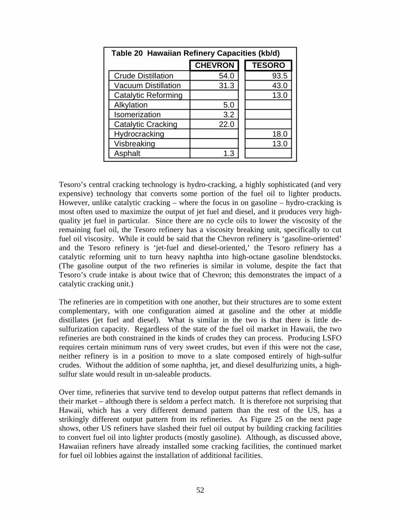
Table 20 Hawaiian Refinery Capacities (kb/d)CHEVRON TESORO

5 93.5 Crude Distillation 4.03 43.0 Vacuum Distillation 1.3

13.0 Catalytic Reforming5 Alkylation .03 Isomerization .2

2 Catalytic Cracking 2.018.0 Hydrocracking13.0 Visbreaking

1 Asphalt .3

Tesoro’s central cracking technology is hydro-cracking, a highly sophisticated (and very expensive) technology that converts some portion of the fuel oil to lighter products. However, unlike catalytic cracking – where the focus in on gasoline – hydro-cracking is most often used to maximize the output of jet fuel and diesel, and it produces very high-quality jet fuel in particular. Since there are no cycle oils to lower the viscosity of the remaining fuel oil, the Tesoro refinery has a viscosity breaking unit, specifically to cut fuel oil viscosity. While it could be said that the Chevron refinery is ‘gasoline-oriented’ and the Tesoro refinery is ‘jet-fuel and diesel-oriented,’ the Tesoro refinery has a catalytic reforming unit to turn heavy naphtha into high-octane gasoline blendstocks. (The gasoline output of the two refineries is similar in volume, despite the fact that Tesoro’s crude intake is about twice that of Chevron; this demonstrates the impact of a catalytic cracking unit.) The refineries are in competition with one another, but their structures are to some extent complementary, with one configuration aimed at gasoline and the other at middle distillates (jet fuel and diesel). What is similar in the two is that there is little de-sulfurization capacity. Regardless of the state of the fuel oil market in Hawaii, the two refineries are both constrained in the kinds of crudes they can process. Producing LSFO requires certain minimum runs of very sweet crudes, but even if this were not the case, neither refinery is in a position to move to a slate composed entirely of high-sulfur crudes. Without the addition of some naphtha, jet, and diesel desulfurizing units, a high-sulfur slate would result in un-saleable products. Over time, refineries that survive tend to develop output patterns that reflect demands in their market – although there is seldom a perfect match. It is therefore not surprising that Hawaii, which has a very different demand pattern than the rest of the US, has a strikingly different output pattern from its refineries. As Figure 25 on the next page shows, other US refiners have slashed their fuel oil output by building cracking facilities to convert fuel oil into lighter products (mostly gasoline). Although, as discussed above, Hawaiian refiners have already installed some cracking facilities, the continued market for fuel oil lobbies against the installation of additional facilities.

52

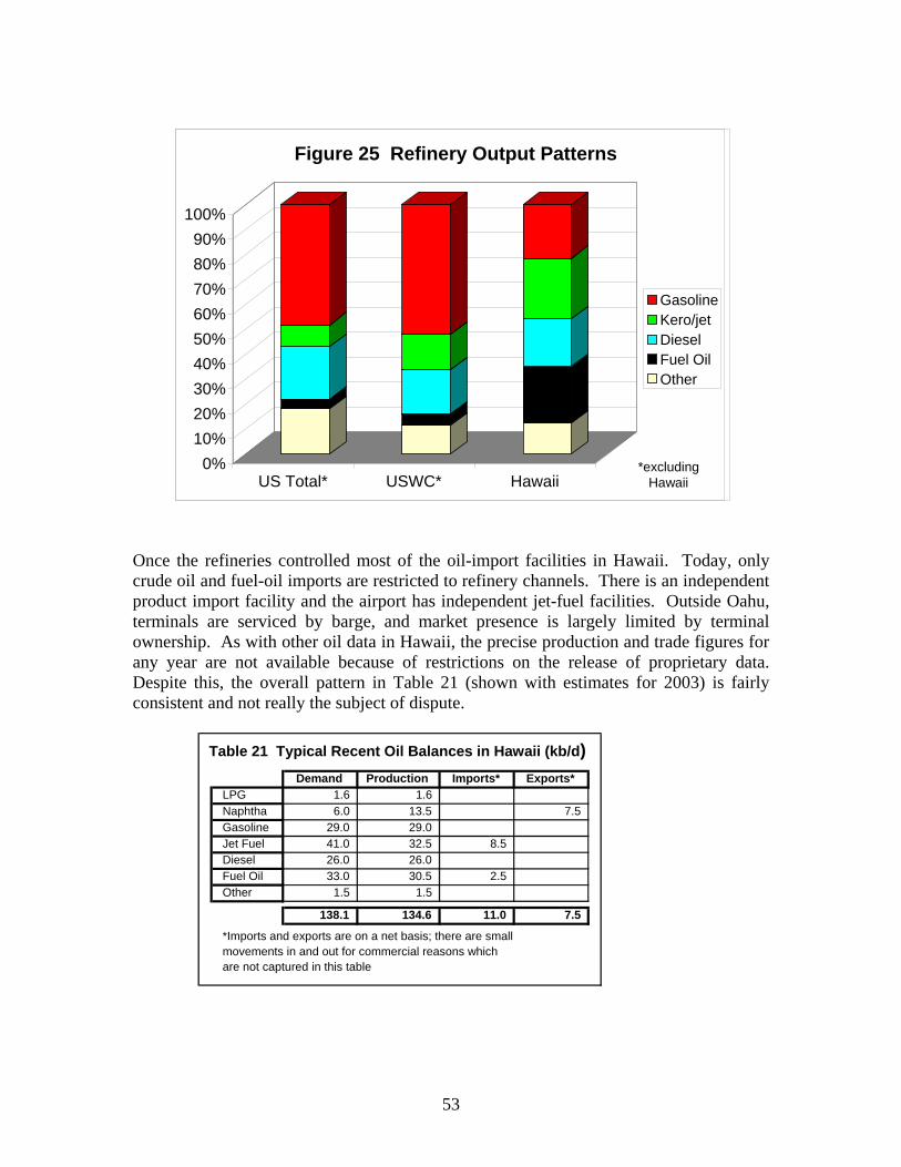
Figure 25 Refinery Output Patterns

100% 90%80%70%

Gasoline60% Kero/jet50% Diesel

Fuel Oil40%Other30%

20%10%

0%

Once the refineries controlled most of the oil-import facilities in Hawaii. Today, only crude oil and fuel-oil imports are restricted to refinery channels. There is an independent product import facility and the airport has independent jet-fuel facilities. Outside Oahu, terminals are serviced by barge, and market presence is largely limited by terminal ownership. As with other oil data in Hawaii, the precise production and trade figures for any year are not available because of restrictions on the release of proprietary data. Despite this, the overall pattern in Table 21 (shown with estimates for 2003) is fairly consistent and not really the subject of dispute.

US Total* USWC* Hawaii*excluding

Hawaii

Table 21 Typical Recent Oil Balances in Hawaii (kb/d)Demand Production Imports* Exports*

LPG 1 .6 1.6 Naphtha 6 .0 1 3.5 7 .5 Gasoline 29 .0 2 9.0 Jet Fuel 41 .0 3 2.5 8 .5

26 .0 2 6.0Diesel Fuel Oil 33 .0 3 0.5 2 .5 Other 1 .5 1.5

13 8.1 1 34.6 1 1.0 7 .5 *Imports and exports are on a net basis; there are smallmovements in and out for commercial reasons whichare not captured in this table

53

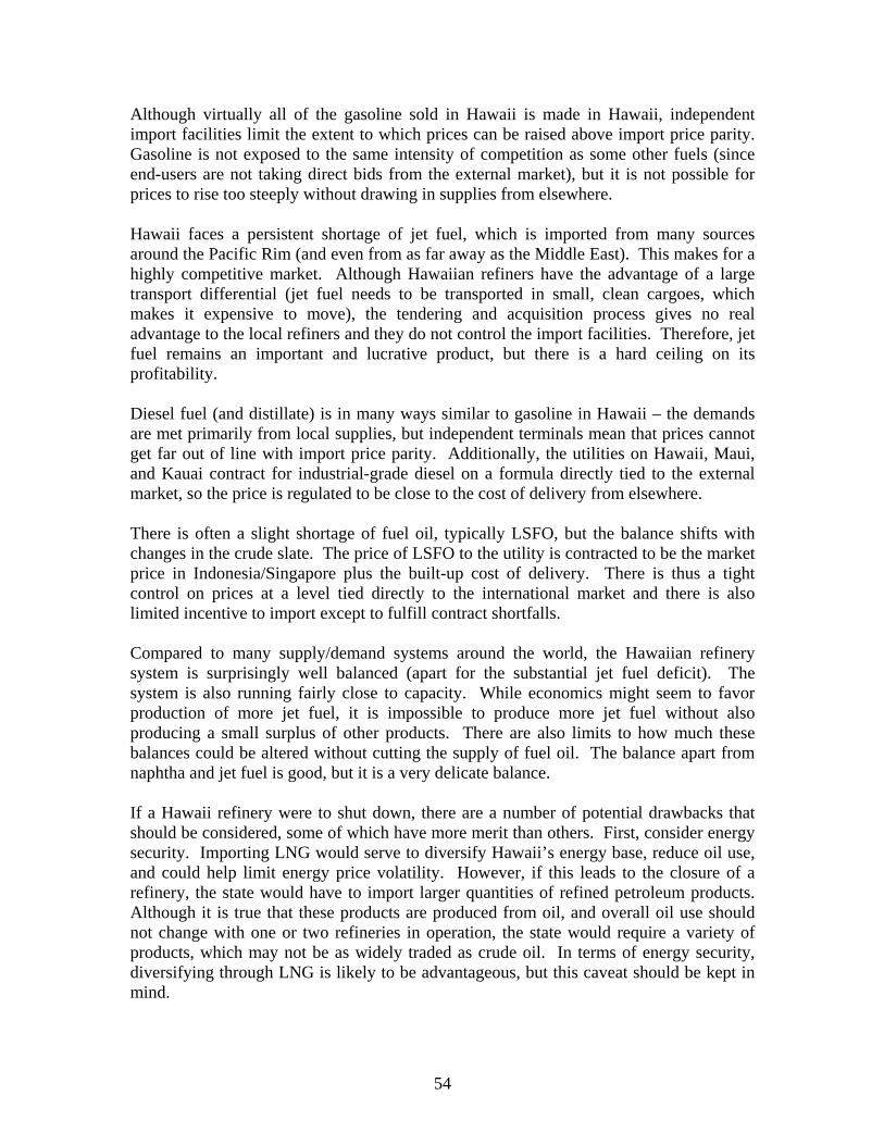
Although virtually all of the gasoline sold in Hawaii is made in Hawaii, independent import facilities limit the extent to which prices can be raised above import price parity. Gasoline is not exposed to the same intensity of competition as some other fuels (since end-users are not taking direct bids from the external market), but it is not possible for prices to rise too steeply without drawing in supplies from elsewhere. Hawaii faces a persistent shortage of jet fuel, which is imported from many sources around the Pacific Rim (and even from as far away as the Middle East). This makes for a highly competitive market. Although Hawaiian refiners have the advantage of a large transport differential (jet fuel needs to be transported in small, clean cargoes, which makes it expensive to move), the tendering and acquisition process gives no real advantage to the local refiners and they do not control the import facilities. Therefore, jet fuel remains an important and lucrative product, but there is a hard ceiling on its profitability. Diesel fuel (and distillate) is in many ways similar to gasoline in Hawaii – the demands are met primarily from local supplies, but independent terminals mean that prices cannot get far out of line with import price parity. Additionally, the utilities on Hawaii, Maui, and Kauai contract for industrial-grade diesel on a formula directly tied to the external market, so the price is regulated to be close to the cost of delivery from elsewhere. There is often a slight shortage of fuel oil, typically LSFO, but the balance shifts with changes in the crude slate. The price of LSFO to the utility is contracted to be the market price in Indonesia/Singapore plus the built-up cost of delivery. There is thus a tight control on prices at a level tied directly to the international market and there is also limited incentive to import except to fulfill contract shortfalls. Compared to many supply/demand systems around the world, the Hawaiian refinery system is surprisingly well balanced (apart for the substantial jet fuel deficit). The system is also running fairly close to capacity. While economics might seem to favor production of more jet fuel, it is impossible to produce more jet fuel without also producing a small surplus of other products. There are also limits to how much these balances could be altered without cutting the supply of fuel oil. The balance apart from naphtha and jet fuel is good, but it is a very delicate balance. If a Hawaii refinery were to shut down, there are a number of potential drawbacks that should be considered, some of which have more merit than others. First, consider energy security. Importing LNG would serve to diversify Hawaii’s energy base, reduce oil use, and could help limit energy price volatility. However, if this leads to the closure of a refinery, the state would have to import larger quantities of refined petroleum products. Although it is true that these products are produced from oil, and overall oil use should not change with one or two refineries in operation, the state would require a variety of products, which may not be as widely traded as crude oil. In terms of energy security, diversifying through LNG is likely to be advantageous, but this caveat should be kept in mind.

54

Nonetheless, having the Oahu fuel-oil demand vanish owing to the import of LNG would change the economic landscape of refining in Hawaii. The first immediate effect would probably be a change in the crude slate, shifting away from such a sweet diet to one higher in sulfur. The second immediate effect would probably be a further shift to light crudes (although the present slate is already fairly light). The third immediate effect would probably be a decline in overall crude runs to avoid large exports of fuel oil – though this would depend heavily on market conditions. In the latter case, it is likely that imports of light products would increase. Thus, several outcomes for the refining industry are possible if the Oahu utility fuels market is eliminated. The industry might retrench and adapt. Modest new investments might be undertaken, possibly over many years, to allow the refiners more flexibility in the crude diet. Or, at the extreme, the industry might be consolidated, expanded, and upgraded to meet the needs of the export market on top of existing local demands. What needs to be stressed is that any of these outcomes is possible with or without the displacement of Oahu’s utility fuel-oil demand. Slashing the demand for LSFO could put new pressure on the refiners (though it also allows them additional room to maneuver), but it is only one of many challenges they face and maintaining the existing market for fuel oil is no guarantee that one or both refiners will continue to operate. To summarize, the closure of one or both refineries is neither inevitable nor does it necessarily lower the competitiveness of the market in Hawaii; indeed, if steps are taken to ensure that a wider selection of fuel suppliers have access to the market (especially in terms of import infrastructure), then price competition might actually be strengthened. It should be noted, however, that this might not happen through purely market forces. The state might have to take a role in ensuring wider access to terminals and tankage. Whether natural gas comes to Hawaii or not in the longer term, both refineries face challenges in terms of changing environmental specifications (sulfur standards continue to tighten everywhere and the refiners have limited ability to cope with these), scale (the refineries are on the small side), and high operating costs (industrial business in Hawaii is difficult). These challenges remain irrespective of natural gas entering Hawaii. 5.0 Conclusions and Comments There are a number of statements that can be made as a result of this study. These will be discussed in terms of the anticipated outcomes and the needs for future analysis, research, and assessment as outlined in the original Scope of Work. First and foremost, it should be understood that, while there are some very useful analyses contained in this report, it is seriously flawed. The primary reason for this serious flaw is that the key point – the economic impact to the state due to changes in oil resource requirements – was not examined. Specifically, there is no true analysis of the impact to the state’s economy based on any one of the three scenarios contained in Section 355. This is due to the lack of information that was able to be obtained for refinery operations due to problems that were outlined in

55

Section 4.4. Thus, any analysis of a scenario would need to be based on a set of assumptions that have not yet been validated. It should be pointed out that the FACTS analysis, in Section 4.3, does provide information on possible outcomes related to at least one of the scenarios. However, a more detailed look at the impact to the state’s economy is lacking and is a serious drawback to the overall study. While not explicitly called for in Section 355, it should also be noted that the scenarios contained within that Section do not provide for an analysis of one of the more obvious sets of approaches for the reduction in petroleum dependency. All of the scenarios are supply-side scenarios and do not address opportunities with demand-side technologies. Specifically, such a scenario would focus on end-use energy efficiency and on peak-demand reduction. Improvements in technologies in both cases would lead to a significant reduction in petroleum demand and dependency. Any future analyses must necessarily examine end-use energy-efficiency scenarios. In addition, no analysis was required for impacts of re-powering existing power plants. This may become an important issue in the future as it may be difficult to get new technologies commercialized. If constraints to siting fossil-fired power plants remain in place, re-powering becomes a viable option, both economically and for the reduction of oil use. Per the original Scope of Work, there are few Category 1 Products that have been produced as part of this analysis. These products were intended to illustrate that sufficient work had been done to preclude a need for further analysis. Certainly, the current state of the state, in terms of energy use and supply, has been examined in detail. However, there is an on-going need to continue to do this work. This is because changes in state policy, in technological advances, in national policy, and in geo-political supply and demand issues require a continual re-evaluation of the state’s energy situation. These analyses must necessarily feed into the development of policies by the state government that would ensure a relatively economic and environmentally-sound approach for maintaining energy supplies in the face of price volatility and security of supplies. Per the Scope of Work, there are a number of Category 2 Products that have been produced as part of this study. These products are defined as those for which there are a sufficient set of data to reach conclusions, but for which additional evaluation or data gathering is required to make the final results more robust. The first product is an acknowledgement that the UHERO models work reasonably well in forecasting future impacts associated with price volatility and increases. However, it is also very clear, after exercising these modeling systems, that additional funding is needed to make them more robust for future analyses that are in the state’s public-goods and public-policy interests. The increased robust nature of these modeling systems can be an important attribute for supporting state policies and increasing the intellectual capacity and technical capabilities of institutions within the state. Per the study in which the UHERO models were utilized, a reasonable set of information was provided (Section 3). It was shown that volatile oil prices appear to have a significant impact on the state economy. Further, for industrial sectors, such as petroleum refining and electricity, it is incorrect to conclude that they will gain from high

56

energy prices, since the analyses determined that these gains in real dollar terms are illusory. It was also illustrated that volatility appeared to have a greater impact on the economy than slow, but steady, increases in oil prices. It should be noted that the comparison of the EIA High case to the baseline case in 2025 shows about a 60% increase in crude oil price. The analysis shows to a 1.5% decline in GSP as a result. This seems to compare closely with the static 50% crude price increase, which shows a GSP loss of 1.4%. This comparison illustrates the similar import of increased petroleum prices in both cases that were evaluated with tow different UHERO models. For the renewable resources for transportation scenario, it was shown that under a certain set of assumptions, ethanol production in the state could provide most, if not all, of the transportation fuel needs for the state. However, these assumptions were made without regard to exogenous requirements, such as those for water, land, and labor. A similar conclusion cannot be reached for biodiesel fuel production. The feedstock that could produce biodiesel for transportations fuels could be grown in the state. However, too little is known about the economics and the related agricultural or aqua-cultural requirements about the feedstock to make an accurate assessment as to the potential for future production for state needs. Additional work would be necessary to evaluate competition for resources and comparative advantages of these technologies. For the liquefied natural gas (LNG) scenario, a rigorous analysis determined that the potential exists for LNG (or CNG) to displace low-sulfur fuel oil as the energy resource for fossil-fired power plants in the state in general and on Oahu in particular. The need for more analysis would center on the economic ability and societal interest to develop the necessary infrastructure to accept LNG, the surety of supplies from foreign sources, and the associated potential of utilizing compressed natural gas due to the need for a smaller investment in infrastructure. For the renewable resources for electricity generation scenario, it was shown that the models such as HOMER, which are transferable to state entities, such as the University of Hawaii, can be used to provide an analysis of renewable energy system penetration for displacement of diesel fuel for small-scale island systems, such as Molokai. This analysis further demonstrated that wind turbines, even with a substantial amount of spinning reserve requirements, could displace diesel on Molokai. However, additional analyses are required in order to determine the impact to grid stability caused by widespread use of intermittent renewable energy systems. The Products listed under Category 3 are, unfortunately, the most important for the overall study. Products that fall into this category are those where sufficiently robust data are lacking that in turn limit any reasonable conclusions or recommendations that would flow from the analysis. There is a domino effect associated with these last two products. Due to the lack of information on refinery impacts, there has been no substantive analytical work performed as part of this study on the effects of any of the scenarios on the operations, economics, and modified product mix associated with either of the state-

57

based refineries. That fact leads to the second product in this category. This is the final integrated analysis, coupled with study recommendations and conclusions. The final analysis was supposed to provide public policy makers with a set of information that could be used to development new policy instruments, as necessary, to reduce the state’s dependence on petroleum, while minimizing exogenous economic impacts that would result from this change in energy resource mix. This analysis could not be done. Lacking this information, there is a clear need to continue these efforts. The lack of support from some groups on the original team notwithstanding, the overall effort allowed for the development of a strong project team that included two University of Hawaii organizations, the National Renewable Energy Laboratory, and FACTS Global Research. It is the bottom-line recommendation of the study that this work be continued to closure with the current study team. This team possesses the requisite skills, expertise, and analytical tools and models to bring the overall effort to a successful close. The result will provide the analysis that was originally intended in the EPACT Section 355 legislation. Specifically, a set of recommendations can be provided to public policy decision-makers for developing new approaches for reducing the dependence of the state on foreign energy supplies and, in the bargain, reduce the state’s overall greenhouse gas emissions.

58

References

1. Macdonald, G. A., A. T. Abbott, and F. L. Peterson., 1984. Volcanoes in the Sea. The Geology of Hawaii, 2nd edition. University of Hawaii Press, Honolulu.

2. State of Hawaii Energy Resources Coordinator Annual Report, 2006. State of Hawaii Department of Business, Economic Development and Tourism, viewed at (http://www.hawaii.gov/dbedt/info/energy/publications/erc06.pdf)

3. U.S. Senators Daniel Akaka and Daniel Inouye, April 26, 2006, letter to U.S. Secretary of Energy Samuel W. Bodman.

4. Energy Policy Act of 2005 (P.L. 109-58).

5. FACTS Global Energy, April 2007. Evaluating Natural Gas Options for the State of Hawaii. Prepared by FACTS Inc. for the Hawaii Natural Energy Institute, subsequently submitted to the State of Hawaii Department of Business, Economic Development and Tourism.

6. Gopalakrishnan, C., X. Tian, and D. Tran,1993. The Impact of Oil-Price Shocks on Hawaii’s Economy: A Case Study Using Vector Autoregression, Energy Systems and Policy 15, 295-305.

7. Keane, M., and E. Prasad,1996. The Employment and Wage Effects of Oil Price changes: A Sectoral Analysis, Review of Economics and Statistics 78(3), 389-400.

8. Huang, B., M.J. Hwang, H. Peng, 2005. The asymmetry of the impact of oil price shocks on economic activities: An application of the multivariate threshold model, Energy Economics 27, 455-476.

9. Cunado, J., F.P. de Gracia, 2005. Oil prices, economic activity and inflation: evidence from some Asian countries, The Quarterly Review of Economics and Finance 48, 65-83.

10 Keffer, V., D. Evans, S. Turn. December 2006. Potential for Ethanol Production in Hawaii. Prepared by the Hawaii Natural Energy Institute for the State of Hawaii Department of Business, Economic Development and Tourism.

11. Anon. 1968-1994. Hawaiian Sugar Manual. Hawaii Sugar Planters' Association, Aiea, HI. 12. Jakeway, L. 2006. Unpublished analysis of sugars in molasses from Hawaiian Commercial & Sugar. Puunene, HI.

13. Shappouri, H. and M. Salassi. 2006. The economic feasibility of ethanol production from sugar in the United States. United States Department of Agriculture, Washington DC.

14. Kinoshita, C. 1988. Composition and processing of burned and unburned cane in Hawaii. International Sugar Journal, (90) 1070, pp. 34-37.

15. Macedo, I., M. Leal, J. Silva. 2004. Assessment of greenhouse gas emissions in the production and use of fuel ethanol in Brazil. Secretariat of the Environment, Government of the State of Sao Paulo, Brazil.

59

16. Aden, A., M. Ruth, K. Ibsen, J. Jechura, K. Neeves, J. Sheehan, B. Wallace, L. Montague, A. Slayton, and J. Lukas. 2002. Lignocellulosic biomass to ethanol process design and economics utilizing co-current dilute acid prehydrolysis and enzymatic hydrolysis for corn stover. National Renewable Energy Laboratory. NREL/TP-510-32438.

17. Sheehan J., A. Aden, K. Paustian, K.. Killian, J. Brenner, M. Walsh, and R. Nelson. 2004. Energy and environmental aspects of using corn stover for fuel ethanol. Journal of Industrial Ecology. Volume 7, No. 3-4, pp. 117-146

18. Anon. 2005. 2005 State of Hawaii Data Book, Section 17: Energy and Science. State of Hawaii, Department of Business, Economic Development & Tourism. Viewed December 27, 2006 at (http://www.hawaii.gov/dbedt/info/economic/databook/db2005/)

19. Anon. 2004. Ethanol Production Costs, A World Wide Survey. F.O. Lichts, Agra Informa Ltd., United Kingdom.

20. Anon. 2006. Recent California reformulated gasoline blendstock prices. California Energy Commission. Viewed at (http://www.energy.ca.gov/gasoline/graphs/component_prices.html)

21. Maloney, W. 2006. Ethanol from sugarcane: A Hawaiian perspective & comparative analysis. Presented at the American Sugar Alliance, 23rd International Sweetner Symposium, August 4-9, 2006.

22. Anon. 2006. AAA's media site for retail gasoline prices. American Automobile Association website. (http://www.fuelgaugereport.com/sbsavg.asp)

23. Hao, S. 2006. Gas tax rising 11¢. Honolulu Advertiser. December 20, 2006. Honolulu, HI.

24. Anon. 2006. Hawaii Biofuel)s Summit Briefing Book. Prepared by the Rocky Mountain Institute for the State of Hawaii Department of Business, Economic Development, & Tourism. Available at: http://www.hawaii.gov/dbedt/info/energy/publications/BiofuelBriefingBook2006.pdf

25. Poteet, Michael D. 2006. Biodiesel Crop Implementation in Hawaii. Prepared by the Hawaii Agriculture Research Center. Aiea, HI for State of Hawaii Department of Agriculture.

26. Anon. 2007. Liquid Fuel Tax Base & Tax Collections, Calendar Year Ending December 31, 2005. Prepared by the Hawaii State Department of Taxation, Tax Research & Planning. Available at: http://www.hawaii.gov/tax/a5_3txcolrptarchive.htm

27. Poteet, Michael D. 2006. Personal communication with S. Turn.

28. Wilson, Christie. 2007. “$61M Biodiesel Plant Outlined.” Honolulu Advertiser. February 18, 2007.

29. Malaysian Palm Oil Board. 2007. Daily Palm Oil Market Price on 03/04/2007. Available at: http://econ.mpob.gov.my/upk/daily/20070403latest.htm.

60

61

30. Anon. 2007a. Annual Report 2006, Country Eligibility for Borrowing from the World Bank. World Bank, Washington DC. Viewed at http://go.worldbank.org/QSMTKY2TE0.

31. Eagar, Harry. 2007. “$61 Million Project a Start to Ending Use of Petroleum.” The Maui News. February 18, 2007. “Energy Company Exploring Oahu for Biodiesel Plant.” The Maui News. April 07, 2007.