Journal of Geodesy (2020) 94:96https://doi.org/10.1007/s00190-020-01424-1

ORIG INAL ART ICLE

Integrated processing of ground- and space-based GPS observations:improving GPS satellite orbits observed with sparse ground networks

Wen Huang1,2 · Benjamin Männel1 · Pierre Sakic1 ·Maorong Ge1,2 · Harald Schuh1,2

Received: 29 January 2019 / Accepted: 19 August 2020 / Published online: 10 October 2020© The Author(s) 2020

AbstractThe precise orbit determination (POD) of Global Navigation Satellite System (GNSS) satellites and low Earth orbiters (LEOs)are usually performed independently. It is a potential way to improve the GNSS orbits by integrating LEOs onboard observa-tions into the processing, especially for the developing GNSS, e.g., Galileo with a sparse sensor station network and Beidouwith a regional distributed operating network. In recent years, few studies combined the processing of ground- and space-basedGNSS observations. The integrated POD of GPS satellites and seven LEOs, including GRACE-A/B, OSTM/Jason-2, Jason-3and, Swarm-A/B/C, is discussed in this study. GPS code and phase observations obtained by onboard GPS receivers of LEOsand ground-based receivers of the International GNSS Service (IGS) tracking network are used together in one least-squaresadjustment. The POD solutions of the integrated processing with different subsets of LEOs and ground stations are analyzedin detail. The derived GPS satellite orbits are validated by comparing with the official IGS products and internal comparisonbased on the differences of overlapping orbits and satellite positions at the day-boundary epoch. The differences between theGPS satellite orbits derived based on a 26-station network and the official IGS products decrease from 37.5 to 23.9mm (34%improvement) in 1D-mean RMS when adding seven LEOs. Both the number of the space-based observations and the LEOorbit geometry affect the GPS satellite orbits derived in the integrated processing. In this study, the latter one is proved tobe more critical. By including three LEOs in three different orbital planes, the GPS satellite orbits improve more than fromadding seven well-selected additional stations to the network. Experiments with a ten-station and regional network show animprovement of the GPS satellite orbits from about 25cm to less than five centimeters in 1D-mean RMS after integrating theseven LEOs.

Keywords POD · Integrated processing · Sparse ground network · GPS · LEOs · GRACE · Jason · Swarm

1 Introduction

The precise orbit determination (POD) of Global Naviga-tion Satellite System (GNSS) satellites is mainly performedwith ground-based observations by a dynamic approach (e.g.,Montenbruck and Gill 2000; Hackel et al. 2015; Zhao et al.2018). The weighted RMS of individual GPS orbit productsprovided by the International GNSS Service (IGS, Johnstonet al. 2018) Analysis Centers with respect to the combined

B Wen Huangwen.huang@gfz-potsdam.de

1 Deutsches GeoForschungsZentrum GFZ, Telegrafenberg14473, Potsdam, Germany

2 Institute of Geodesy and Geoinformation Science, TechnischeUniversität Berlin, Strasse des 17. Juni 135, Berlin 10623,Germany

solution is 6.3mm to 11mm (Choi 2014). Orbits of lowEarthorbiters (LEOs) are usually determined by introducing GPSorbit and clock products to process the onboard GNSS obser-vations. With a reduced dynamic strategy (Wu et al. 1991),the orbits of different LEOs are determined to an accuracylevel of one to three centimeters (e.g., Haines et al. 2004;Jäggi et al. 2007; Montenbruck et al. 2018).

There are also some studies on the integrated processing ofground- and space-based observations, mainly focusing onthe estimation of Earth parameters, including gravity fieldparameters (König et al. 2005), the geocenter (Kuang et al.2015; Männel and Rothacher 2017), and the terrestrial ref-erence frame (König 2018). The integrated POD of GPSsatellites and LEOs was also performed by several studies.Zhu et al. (2004) and König et al. (2005) compared twoPOD approaches for GPS, the Gravity Recovery and ClimateExperiment (GRACE), and the Challenging Minisatellite

123

96 Page 2 of 13 W. Huang et al.

Payload (CHAMP) satellites. In the first approach named‘one-step’, the orbits of the above-mentioned satellites areestimated simultaneously. In the other approach, the orbitsof the GPS satellites and the LEOs are determined sequen-tially. The authors concluded that the orbits determined bythe ‘one-step’ approach aremore accurate. Geng et al. (2008)shown that the GPS satellite orbits derived by supplement-ing a 21-station networkwithGRACEandCHAMP satellitesare more accurate than the solution based on a 43-station net-work. Otten et al. (2012) combined various GNSS satellitesand LEOs at the observation level including GNSS, DopplerOrbitography and Radiopositioning Integrated by Satellite(DORIS), and Satellite Laser Ranging (SLR). Zoulida et al.(2016) and Zhao et al. (2017) performed an integrated PODfor OSTM/Jason-2 and FengYun-3C with GPS and Beidou,respectively. These studies reported the benefits of integrat-ing LEOs into the POD in different aspects. However, onlyone or two LEO missions that have GNSS data were consid-ered in the above-mentioned studies.

In this study, we considered seven LEOs, includingGRACE-A, GRACE-B, OSTM/Jason-2, Jason-3, Swarm-A,Swarm-B, andSwarm-C. For the selection of ground stations,the characteristics of the ground segments ofGalileo andBei-dou are taken into consideration. The Galileo Sensor Station(GSS) network includes 16 sites (Sakic et al. 2018) and Bei-dou has a regionally distributed ground segment (Yang2018).It is a potential way to supplement the limited ground seg-ment by integrating LEOs in joint POD processing. Basedon the integrated processing of different subsets of groundstations and LEOs, the impact of integrating LEOs on theGPS satellite orbits is discussed.

In Sect. 2, the integrated processing is introduced briefly.The characteristics of the LEOs and their data selection arepresented. The processing days are selected based on thedata status of the LEOs. Two main sparse subsets of theavailable IGS stations are selected based on the motivationof our study. The strategy of our processing and analysisand all the designed scenarios are explained in detail. Allthe results and analysis are given in Sect. 3. It includesfour parts. Firstly, the impact of the number of LEOs andtheir orbital planes on GPS satellite orbits is discussed. Sec-ondly, internal comparisons of the orbit quality based on thedifferences of overlapping orbits and satellite positions atday-boundary epochs are performed. Thirdly, the effects ofsupplementing a sparse and non-homogeneously distributedstation network by seven carefully selected additional sta-tions or three LEOs in different orbital planes are compared.Fourthly, we present an additional experiment to show theGPS satellite orbit improvement by adding seven LEOs to aregional ground network. The conclusions are given basedon the above-mentioned results and analysis in Sect. 4.

2 Integrated POD of GPS satellites and LEOs

2.1 Themethod of integrated POD

The method of the integrated POD applied in this study isknown as the one-stepmethod (Montenbruck and Gill 2000).The approximate initial epoch status of GPS satellites andLEOs are computed from broadcast ephemerides and by sin-gle point positioning, respectively. Based on the equations ofmotion of GPS satellites and LEOs, the initial orbits of GPSand LEOs are delivered by numerical integration. The stateequation reads

xi = T (ti , t0)x0 + S(ti , t0) f , (1)

where xi is the state vector of the satellite at epoch ti , x0 is theinitial epoch state vector, f contains the force model param-eters, and T (ti , t0) and S(ti , t0) are transition matrices andsensitivity matrices, respectively. In the one-step estimation,the ground- and space-based observation equations at epochti read

Lgpssta = Fgps

sta (xgps, xsta,Cgps, csta, T

gpssta , I gpssta , Agps

sta , ti )

+ vgpssta ,

Lgpsleo = Fleo

sta (xleo, xgps,Cgps, cleo, T

gpsleo , I gpsleo , Agps

leo , ti )

+ vgpsleo , (2)

where Lsta and Lleo are ground- and space-based measure-ments, xgps and xleo are the positions of GPS satellites andLEOs at the current epoch, xsta is the static position ofthe ground station, c denotes the receiver clock offset, Cdenotes the GPS satellite clock offset, T is the tropospheredelay, I is the ionosphere delay, Agps

sta and Agpsleo are carrier

phase ambiguities of stations and LEOs, and vgpssta and v

gpsleo

contain unmodeled effects andmeasurement errors. The esti-mation is performed by inserting Eq. 1 to linearized Eq. 2.The accurate initial epoch states and force model parametersof GPS satellites and LEOs are estimated in a least-squaresadjustment by using ground-based and LEOs onboard obser-vations simultaneously. It has to bementioned thatwe formedionosphere-free linear combinations of the measurements.

Figure 1 presents the flowchart of the whole process-ing. Before the one-step estimation, all the observations arecleaned based on the TurboEdit algorithm (Blewitt 1990).Several iterations of estimation are performed to improve thesolution. After each estimation, the orbits of GPS satellitesand LEOs are updated by orbit integration based on the newsolution of initial epoch states and force model parameters.Meanwhile, the data are cleaned based on the residuals ofobservations. After completing the data cleaning, the ambi-guities of the ground station observations are fixed to improvethe solution. After one more iteration of estimation and orbit

123

Integrated processing of ground- and space-based GPS observations: improving GPS… Page 3 of 13 96

GPSbroadcastephemeris

Ground- andSpace-based GPS

observations

Initial orbitspreparation

Data cleaningbased on turboedit

Initial dynamicorbits of GPS and

LEO satellites

Cleanedobservations

Least squares estimation

Orbits updating

Updated orbits

Data cleaningbased on residuals

Data cleaningcompleted?

Ground station ambiguity fixing

Least squares estimation

Orbits updating

Final orbits of GPS and LEO satellites

No

Yes

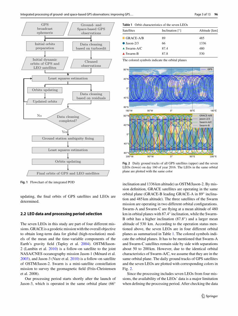
Fig. 1 Flowchart of the integrated POD

updating, the final orbits of GPS satellites and LEOs aredetermined.

2.2 LEO data and processing period selection

The seven LEOs in this study are part of four different mis-sions.GRACE is ageodeticmissionwith theoverall objectiveto obtain long-term data for global (high-resolution) mod-els of the mean and the time-variable components of theEarth’s gravity field (Tapley et al. 2004). OSTM/Jason-2 (Lambin et al. 2010) is a follow-on satellite to the jointNASA/CNES oceanography mission Jason-1 (Ménard et al.2003), and Jason-3 (Vaze et al. 2010) is a follow-on satelliteof OSTM/Jason-2. Swarm is a mini-satellite constellationmission to survey the geomagnetic field (Friis-Christensenet al. 2008).

Our processing period starts shortly after the launch ofJason-3, which is operated in the same orbital plane (66◦

Table 1 Orbit characteristics of the seven LEOs

Satellites Inclination [◦] Altitude [km]

GRACE-A/B 89 485

Jason-2/3 66 1336

Swarm-A/C 87.4 480

Swarm-B 87.8 530

The colored symbols indicate the orbital planes

Fig. 2 Daily ground tracks of all GPS satellites (upper) and the sevenLEOs (lower) on day 160 of year 2016. The LEOs in the same orbitalplane are plotted with the same color

inclination and 1336km altitude) as OSTM/Jason-2. Bymis-sion definition, GRACE satellites are operating in the sameorbital plane (GRACE-B leading GRACE-A in 89◦ inclina-tion and 485km altitude). The three satellites of the Swarmmission are operating in two different orbital configurations.Swarm-A and Swarm-C are flying at a mean altitude of 480km in orbital planes with 87.4◦ inclination, while the Swarm-B orbit has a higher inclination (87.8◦) and a larger meanaltitude of 530 km. According to the operation status men-tioned above, the seven LEOs are in four different orbitalplanes as summarized in Table 1. The colored symbols indi-cate the orbital planes. It has to be mentioned that Swarm-Aand Swarm-C satellites remain side by side with separationsabout 50 to 200km. However, due to the identical orbitalcharacteristics of Swarm-A/C, we assume that they are in thesame orbital plane. The daily ground tracks of GPS satellitesand the seven LEOs are plotted with corresponding colors inFig. 2.

Since the processing includes seven LEOs from four mis-sions, the availability of the LEOs’ data is a major limitationwhen defining the processing period. After checking the data

123

96 Page 4 of 13 W. Huang et al.

Fig. 3 Status of data availability in the processing period

Table 2 The RMS of the orbit differences between our LEO PODsolutions and the official orbit products averaged over 112 processeddays

LEO G-A G-B J-2 J-3 S-A S-B S-C

RMS [mm] 33.0 36.3 37.5 42.0 33.5 33.5 33.8

The daily RMS is computed over epochs and three orbital directions(along-track, cross-track, and radial)

availability of the seven LEOs, we choose day of year (DOY)115 to 260 in 2016 as our processing period. In this period, allseven LEOs were in operation. GRACE satellites were at theend of their operating life, but the quaternion data of Jason-3started to be available from DOY 115 in 2016. To check theLEOs’ data quality, a daily POD of each LEO is processedwith a 300-second data sampling rate. The IGS final orbitand clock products are introduced as a priori information.We noticed missing data (onboard GPS observation or atti-tude) for some days. Some additional days were excluded formaneuvering or low data quality caused by spacecraft prob-lems. Please note thatwe excluded these days completely alsoin the following integrated processing. In the integrated pro-cessing, we also excluded maneuvering GPS satellites basedon the information provided in the GPS NANU Messages.Finally, 112 days are selected for the integrated processingand are indicated by green dots in Fig. 3. The LEOs’ dailyorbits are compared with the official orbit products (Caseet al. 2002; Dumont et al. 2009, 2016; Olsen 2019). TheRMS of the orbit differences is computed over the epochsand three orbital directions in a daily solution. The averageof the daily RMS values over the 112 days are presented inTable 2. We abbreviate the LEOs as G-A/B (GRACE-A/B),J-2/3 (OSTM/Jason-2 and Jason3), and S-A/B/C (Swarm-A/B/C). The larger RMS of Jason-3 compared to that ofOSTM/Jason-2 is related to orbit modeling issues, as weapplied the model of OSTM/Jason-2 to Jason-3, since somedetailed information of Jason-3, for instance, the receiverantenna phase center location, are not yet available. Com-pared with previous studies and considering the 300-seconddata sampling rate, a comparable accuracy level of the LEOorbits is achieved.

Fig. 4 Available IGS stations (in total 319) for the 112 selected pro-cessing days

Fig. 5 A subset of the available IGS stations including 33 homoge-neously and sparsely distributed stations (blue triangles). The numberof stations in sight of a potential GPS satellite position (Depth of Cov-erage) is presented as a colored bin (2◦ × 2◦ resolution, 20,200kmaltitude)

2.3 Ground networks selection

There are 319 IGS stations available during the selected 112processing days. The distribution of the 319 stations is pre-sented in Fig. 4. The operation of allGNSS ismainly based ontheir own ground segments and tracking stations. For exam-ple, as mentioned in Sect. 1, there are only 16 sites withGSS operating for Galileo. Considering this situation, weselected a sparse and homogeneously distributed subset fromthe 319 available IGS stations to study the sparse-network-based POD. This network contains 33 stations which areplotted as blue triangles in Fig. 5. The color of the bins inFigs. 5 and 6 presents the number of stations in sight of apotentialGPS satellite positionwith an altitude of 20, 200kmand an inclination of 57◦ (i.e., Depth of Coverage, DoC). Ingeneral, more than five stations are visible, and this is alsowhat we expected based on the selection criteria.

Despite the large and dense IGS tracking network incertain circumstances, depending on constellations and fre-quencies, onemight be confrontedwith large regionswithouttracking stations, especially over the oceans andAfrica. Seenfrom Fig. 4, although 319 stations are globally available,there are regions with only a few tracking stations. More-over, IGS stations could be unavailable for various reasons,

123

Integrated processing of ground- and space-based GPS observations: improving GPS… Page 5 of 13 96

Fig. 6 A subset of the available IGS stations including 26 non-homogeneously and sparsely distributed stations (blue triangles). Thered triangles are the seven excluded stations. The number of stationsin sight of a potential GPS satellite position (Depth of Coverage) ispresented as a colored bin (2◦ × 2◦ resolution, 20,200km altitude)

and it might happen to Galileo Sensor Stations as well, forinstance, caused by the withdrawal of the United Kingdomfrom the European Union (Gutierrez 2018). To investigatehow the LEOs could contribute to the GPS POD, we selecteda sparser station network (see Fig. 6) by excluding seven (redtriangles) of the 33 stations mentioned above. Consequently,gaps in some regions of the Pacific Ocean, the Indian Ocean,and Africa are visible. There are large areas where a fictitiousGPS satellite could be tracked by only two to four (yellowbins) stations. Although two simultaneous observations cansupport the estimation of satellite clock corrections and orbitparameters in a dynamic solution, the fewer observations stilllead to a reduced contribution.

The GPS satellite orbits derived from the two sparse net-works mentioned above are our benchmark which will becompared with different integrated solutions. All selectedstations are used to define the datum. Since we applied aHelmert transformation when comparing our orbits with theIGS final products, there will be little systematic effect whenwe analyze the RMS of the orbit differences compared tothese two benchmark results.

To investigate the performance of the integrated PODwithregional networks, another network including stationsmainlylocated in China will be introduced in Sect. 3.4.

2.4 Processing and analysis strategy

We use the software PANDA (Liu and Ge 2003) to doall the processing. PANDA is capable of GNSS satelliteand LEO orbit modeling. Separated and integrated POD ofGNSS satellites and LEOs can be performed. For this study,the implementation of OSTM/Jason-2, Jason-3, and Swarm-A/B/C data formats (observation, attitude, and precise orbit)was necessary. Table 3 shows the dynamic models used forthe orbit integration of GPS satellites and LEOs. Table 4introduces the processing configuration and the estimatedparameters.

To investigate the impact of the number of integratedLEOs and their orbital planes on the determinedGPS satelliteorbits,we applied a total of 26 different scenarios for the PODprocessing. All the scenarios are summarized in Table 5. Thefirst two are the GPS-only POD by applying the two sparsestation networks which are described in Sect. 2.3. The other24 scenarios are the integrated POD of GPS satellites andLEOs, and all of them supplement the sparser network with26 stations by including different subsets of the seven LEOs.We compared the estimated GPS satellite orbits of all scenar-ios to the IGS final products to show the orbit quality and thedifferences between the scenarios. Due to the large numberof satellites and scenarios, we computed statistical measuresof the orbit comparisons to quantify the result of each sce-nario. The statistical computation is shown in Fig. 7. For eachdaily orbit comparison, we computed the RMS of orbit dif-ferences in three orbital directions (along-track, cross-track,and radial) and the 1D-mean RMS. The RMS in three orbitaldirections is computed over epochs and satellites. The 1D-mean RMS is computed over epochs, satellites, and the threeorbital directions. Based on the 112-day solutions, we com-puted the mean and the empirical standard deviation of thetime series of the above-mentioned RMS values. The statis-tical measures mentioned above are highlighted in green inFig. 7, and the analysis in Sect. 3.1 is mainly based on thesemeasures.

Besides the external orbit comparison, internal compar-isons are performed in two different ways. The first one is

Table 3 Dynamic orbit models of GPS satellites and LEOs

Dynamic Models GPS LEOs

Atmosphere drag Not applied DTM94 (Berger et al. 1998)

Earth gravity field EIGEN-GRACE02S (12 × 12, Reigber et al. 2005) EIGEN-GRACE02S (120 × 120)

Earth radiation pressure Box-wing (Marshall et al. 1992) Not applied

N-body perturbation JPL DE405 (Standish 1998) JPL DE405

Relativity IERS 2010 (Petit and Luzum 2010) IERS 2010

Solid Earth, ocean, pole tide IERS 2010 IERS 2010

Solar radiation pressure reduced ECOM (Springer et al. 1999) Box-wing

123

96 Page 6 of 13 W. Huang et al.

Table 4 Processing configurations and estimated parameters

Arc length 24 hours (expanding 3 hours to the previous and the next day for overlapping comparison)

Cut-off elevation 7◦

GPS Antenna PCO/PCV IGS08.atx (Schmid et al. 2016)

LEOs Antenna PCO/PCV PCO values are offered by mission operators, and PCV is not applied

LEOs attitude Quaternion data provided by mission operators

Observation type Undifferenced ionosphere-free phase and code measurements

Weighting Ground and space-based observations are equally weighted

Sampling rate Five minutes for both ground and onboard observations

Datum definition IGS weekly solution of station coordinates aligned to ITRF2008 (Rebischung et al. 2012)

Ambiguity fixing Only within ground stations

Parameters

Station coordinate Highly constrained

GPS satellite orbit Six orbital elements and five solar radiation pressure parameters

LEOs orbit Six orbital elements; piece-wise empirical and atmosphere drag parameters

Earth rotation Rotation pole coordinates and UT1 for 24h intervals; piece-wise linear modeling

Tropospheric delay For each ground station; piece-wise constant zenith delays for 1h intervals; piece-wise constant horizontalgradients for 4h intervals

Phase ambiguities Fixed for ground observations; float for space-based observations

Clock offsets Satellites and receivers; epoch-wise; pre-eliminated

IGS finalorbit products

GPS satellite orbitdaily solutions

Orbit comparison

Epochwise orbit differences inthree directions of each satellite

Root mean squareover epochs

Root mean squareover epochs, direc-tions and satellites

1D-RMS ofeach satellite inthree directions

1D-mean RMS

Root mean squareover satellites

Times series(mean and stan-dard deviation)

AlongRMS

CrossRMS

RadialRMS

epoch-wise orbit differ-ences of each satellite

Fig. 7 Flowchart of the statistical computation. The green and yellowoutputs are the values used in the analysis of this study

the comparison of the orbit overlaps.We expand the POD arclength of scenarios 1, 2, and 26 from 24 hours to 30 hours(three hours to both the previous and the next day). Conse-quently, a pair of 6-hour overlapping orbit arcs derived by realdata processing is generated between two adjacent days. The1D-mean RMS of the orbit differences of the 6-hour overlapis computed. Another comparison is about the satellite posi-tion differences at the day-boundary epoch of two adjacent24-hour orbits at midnight. We extrapolate one more epochfrom a 24-hour orbit by orbit integration, then the GPS satel-lite positions at the extrapolated epoch are compared withthe estimated satellite positions in the first epoch of the next24-hour orbit. The RMS of the satellite position differencesis computed over the satellites and the three orbital directionsat the day-boundary epochs. The detailed discussion will begiven in Sect. 3.2.

Based on a geolocated comparison of epoch-wise satelliteorbit differences (yellow box in Fig. 7) between scenarios1, 2, and 19, we will discuss the different effects of sup-plementing a sparse station network with additional stationsand LEOs in Sect. 3.3. An additional experiment is designedto show the GPS satellite orbit improvement by adding theseven LEOs to a small and mainly regionally distributed sta-tion network. The 1D-mean RMS of the GPS satellite orbitdifferences compared to IGS final products will be used forthe analysis in Sect. 3.4.

123

Integrated processing of ground- and space-based GPS observations: improving GPS… Page 7 of 13 96

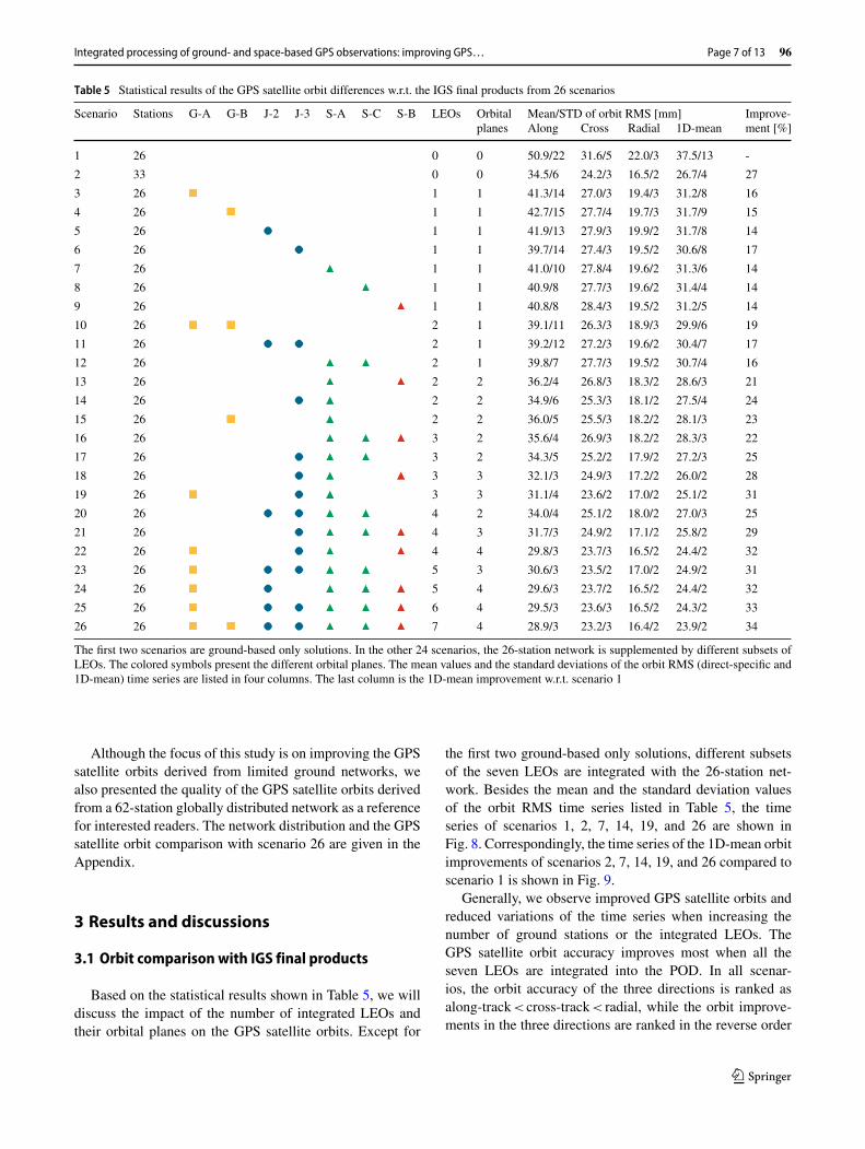
Table 5 Statistical results of the GPS satellite orbit differences w.r.t. the IGS final products from 26 scenarios

Scenario Stations G-A G-B J-2 J-3 S-A S-C S-B LEOs Orbital Mean/STD of orbit RMS [mm] Improve-planes Along Cross Radial 1D-mean ment [%]

1 26 0 0 50.9/22 31.6/5 22.0/3 37.5/13 -

2 33 0 0 34.5/6 24.2/3 16.5/2 26.7/4 27

3 26 1 1 41.3/14 27.0/3 19.4/3 31.2/8 16

4 26 1 1 42.7/15 27.7/4 19.7/3 31.7/9 15

5 26 1 1 41.9/13 27.9/3 19.9/2 31.7/8 14

6 26 1 1 39.7/14 27.4/3 19.5/2 30.6/8 17

7 26 1 1 41.0/10 27.8/4 19.6/2 31.3/6 14

8 26 1 1 40.9/8 27.7/3 19.6/2 31.4/4 14

9 26 1 1 40.8/8 28.4/3 19.5/2 31.2/5 14

10 26 2 1 39.1/11 26.3/3 18.9/3 29.9/6 19

11 26 2 1 39.2/12 27.2/3 19.6/2 30.4/7 17

12 26 2 1 39.8/7 27.7/3 19.5/2 30.7/4 16

13 26 2 2 36.2/4 26.8/3 18.3/2 28.6/3 21

14 26 2 2 34.9/6 25.3/3 18.1/2 27.5/4 24

15 26 2 2 36.0/5 25.5/3 18.2/2 28.1/3 23

16 26 3 2 35.6/4 26.9/3 18.2/2 28.3/3 22

17 26 3 2 34.3/5 25.2/2 17.9/2 27.2/3 25

18 26 3 3 32.1/3 24.9/3 17.2/2 26.0/2 28

19 26 3 3 31.1/4 23.6/2 17.0/2 25.1/2 31

20 26 4 2 34.0/4 25.1/2 18.0/2 27.0/3 25

21 26 4 3 31.7/3 24.9/2 17.1/2 25.8/2 29

22 26 4 4 29.8/3 23.7/3 16.5/2 24.4/2 32

23 26 5 3 30.6/3 23.5/2 17.0/2 24.9/2 31

24 26 5 4 29.6/3 23.7/2 16.5/2 24.4/2 32

25 26 6 4 29.5/3 23.6/3 16.5/2 24.3/2 33

26 26 7 4 28.9/3 23.2/3 16.4/2 23.9/2 34

The first two scenarios are ground-based only solutions. In the other 24 scenarios, the 26-station network is supplemented by different subsets ofLEOs. The colored symbols present the different orbital planes. The mean values and the standard deviations of the orbit RMS (direct-specific and1D-mean) time series are listed in four columns. The last column is the 1D-mean improvement w.r.t. scenario 1

Although the focus of this study is on improving the GPSsatellite orbits derived from limited ground networks, wealso presented the quality of the GPS satellite orbits derivedfrom a 62-station globally distributed network as a referencefor interested readers. The network distribution and the GPSsatellite orbit comparison with scenario 26 are given in theAppendix.

3 Results and discussions

3.1 Orbit comparison with IGS final products

Based on the statistical results shown in Table 5, we willdiscuss the impact of the number of integrated LEOs andtheir orbital planes on the GPS satellite orbits. Except for

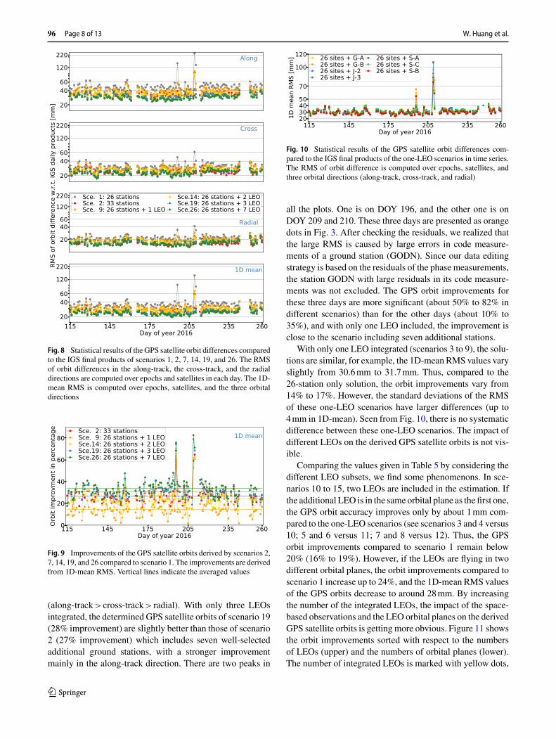
the first two ground-based only solutions, different subsetsof the seven LEOs are integrated with the 26-station net-work. Besides the mean and the standard deviation valuesof the orbit RMS time series listed in Table 5, the timeseries of scenarios 1, 2, 7, 14, 19, and 26 are shown inFig. 8. Correspondingly, the time series of the 1D-mean orbitimprovements of scenarios 2, 7, 14, 19, and 26 compared toscenario 1 is shown in Fig. 9.

Generally, we observe improved GPS satellite orbits andreduced variations of the time series when increasing thenumber of ground stations or the integrated LEOs. TheGPS satellite orbit accuracy improves most when all theseven LEOs are integrated into the POD. In all scenar-ios, the orbit accuracy of the three directions is ranked asalong-track<cross-track< radial, while the orbit improve-ments in the three directions are ranked in the reverse order

123

96 Page 8 of 13 W. Huang et al.

Fig. 8 Statistical results of the GPS satellite orbit differences comparedto the IGS final products of scenarios 1, 2, 7, 14, 19, and 26. The RMSof orbit differences in the along-track, the cross-track, and the radialdirections are computed over epochs and satellites in each day. The 1D-mean RMS is computed over epochs, satellites, and the three orbitaldirections

Fig. 9 Improvements of the GPS satellite orbits derived by scenarios 2,7, 14, 19, and 26 compared to scenario 1. The improvements are derivedfrom 1D-mean RMS. Vertical lines indicate the averaged values

(along-track>cross-track> radial). With only three LEOsintegrated, the determined GPS satellite orbits of scenario 19(28% improvement) are slightly better than those of scenario2 (27% improvement) which includes seven well-selectedadditional ground stations, with a stronger improvementmainly in the along-track direction. There are two peaks in

Fig. 10 Statistical results of the GPS satellite orbit differences com-pared to the IGS final products of the one-LEO scenarios in time series.The RMS of orbit difference is computed over epochs, satellites, andthree orbital directions (along-track, cross-track, and radial)

all the plots. One is on DOY 196, and the other one is onDOY 209 and 210. These three days are presented as orangedots in Fig. 3. After checking the residuals, we realized thatthe large RMS is caused by large errors in code measure-ments of a ground station (GODN). Since our data editingstrategy is based on the residuals of the phase measurements,the station GODN with large residuals in its code measure-ments was not excluded. The GPS orbit improvements forthese three days are more significant (about 50% to 82% indifferent scenarios) than for the other days (about 10% to35%), and with only one LEO included, the improvement isclose to the scenario including seven additional stations.

With only one LEO integrated (scenarios 3 to 9), the solu-tions are similar, for example, the 1D-mean RMS values varyslightly from 30.6mm to 31.7mm. Thus, compared to the26-station only solution, the orbit improvements vary from14% to 17%. However, the standard deviations of the RMSof these one-LEO scenarios have larger differences (up to4mm in 1D-mean). Seen from Fig. 10, there is no systematicdifference between these one-LEO scenarios. The impact ofdifferent LEOs on the derived GPS satellite orbits is not vis-ible.

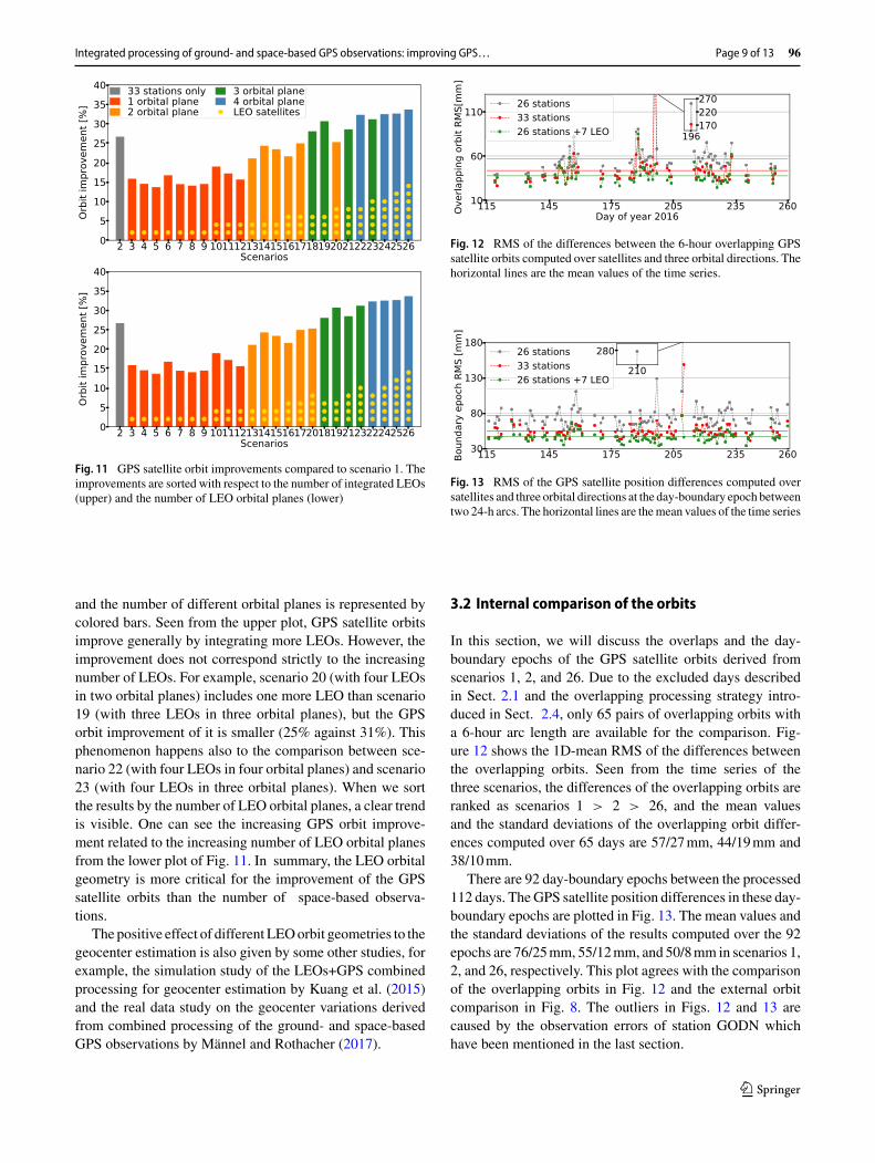
Comparing the values given in Table 5 by considering thedifferent LEO subsets, we find some phenomenons. In sce-narios 10 to 15, two LEOs are included in the estimation. Ifthe additional LEO is in the same orbital plane as the first one,the GPS orbit accuracy improves only by about 1mm com-pared to the one-LEO scenarios (see scenarios 3 and 4 versus10; 5 and 6 versus 11; 7 and 8 versus 12). Thus, the GPSorbit improvements compared to scenario 1 remain below20% (16% to 19%). However, if the LEOs are flying in twodifferent orbital planes, the orbit improvements compared toscenario 1 increase up to 24%, and the 1D-mean RMS valuesof the GPS orbits decrease to around 28mm. By increasingthe number of the integrated LEOs, the impact of the space-based observations and the LEO orbital planes on the derivedGPS satellite orbits is getting more obvious. Figure 11 showsthe orbit improvements sorted with respect to the numbersof LEOs (upper) and the numbers of orbital planes (lower).The number of integrated LEOs is marked with yellow dots,

123

Integrated processing of ground- and space-based GPS observations: improving GPS… Page 9 of 13 96

Fig. 11 GPS satellite orbit improvements compared to scenario 1. Theimprovements are sorted with respect to the number of integrated LEOs(upper) and the number of LEO orbital planes (lower)

and the number of different orbital planes is represented bycolored bars. Seen from the upper plot, GPS satellite orbitsimprove generally by integrating more LEOs. However, theimprovement does not correspond strictly to the increasingnumber of LEOs. For example, scenario 20 (with four LEOsin two orbital planes) includes one more LEO than scenario19 (with three LEOs in three orbital planes), but the GPSorbit improvement of it is smaller (25% against 31%). Thisphenomenon happens also to the comparison between sce-nario 22 (with four LEOs in four orbital planes) and scenario23 (with four LEOs in three orbital planes). When we sortthe results by the number of LEO orbital planes, a clear trendis visible. One can see the increasing GPS orbit improve-ment related to the increasing number of LEO orbital planesfrom the lower plot of Fig. 11. In summary, the LEO orbitalgeometry is more critical for the improvement of the GPSsatellite orbits than the number of space-based observa-tions.

The positive effect of different LEOorbit geometries to thegeocenter estimation is also given by some other studies, forexample, the simulation study of the LEOs+GPS combinedprocessing for geocenter estimation by Kuang et al. (2015)and the real data study on the geocenter variations derivedfrom combined processing of the ground- and space-basedGPS observations by Männel and Rothacher (2017).

Fig. 12 RMS of the differences between the 6-hour overlapping GPSsatellite orbits computed over satellites and three orbital directions. Thehorizontal lines are the mean values of the time series.

Fig. 13 RMS of the GPS satellite position differences computed oversatellites and three orbital directions at the day-boundary epoch betweentwo 24-h arcs. The horizontal lines are themean values of the time series

3.2 Internal comparison of the orbits

In this section, we will discuss the overlaps and the day-boundary epochs of the GPS satellite orbits derived fromscenarios 1, 2, and 26. Due to the excluded days describedin Sect. 2.1 and the overlapping processing strategy intro-duced in Sect. 2.4, only 65 pairs of overlapping orbits witha 6-hour arc length are available for the comparison. Fig-ure 12 shows the 1D-mean RMS of the differences betweenthe overlapping orbits. Seen from the time series of thethree scenarios, the differences of the overlapping orbits areranked as scenarios 1 > 2 > 26, and the mean valuesand the standard deviations of the overlapping orbit differ-ences computed over 65 days are 57/27mm, 44/19mm and38/10mm.

There are 92 day-boundary epochs between the processed112 days. TheGPS satellite position differences in these day-boundary epochs are plotted in Fig. 13. The mean values andthe standard deviations of the results computed over the 92epochs are 76/25mm, 55/12mm, and 50/8mm in scenarios 1,2, and 26, respectively. This plot agrees with the comparisonof the overlapping orbits in Fig. 12 and the external orbitcomparison in Fig. 8. The outliers in Figs. 12 and 13 arecaused by the observation errors of station GODN whichhave been mentioned in the last section.

123

96 Page 10 of 13 W. Huang et al.

Fig. 14 GPS satellite orbit improvements of scenarios 2 w.r.t. scenario1. IGS final products are reference. The color of each bin presents theaverage value of the epoch-wise solutions located in the bin. The unitof the color bar is [mm]

Fig. 15 GPS satellite orbit improvements of scenarios 19w.r.t. scenario1. IGS final products are reference. The color of each bin presents theaverage value of the epoch-wise solutions located in the bin. The unitof the color bar is [mm]

3.3 Geolocated visualization of orbit comparison

In Sect. 2.3, we explained that the seven additional stationsin scenario 2 were selected in the regions with few stationsin scenario 1. For the analysis regarding station distributions,the GPS satellite orbit improvements of scenarios 2 and 19compared to scenario 1 are projected to the surface of theEarth. Based on the epoch-wise orbit difference of each GPSsatellite compared to the IGSfinal products, we computed theimprovements of theGPSsatellite orbits of scenarios 2 and19compared to scenario 1 with a 900-second sampling rate forall GPS satellites in 112 days (approximate 344,064 epoch-wise solutions). The results are presented in Figs. 14 and 15.In these two figures, the potential GPS satellite position areais divided into geographical 2◦ × 2◦ bins (10,260 in total).We computed the average of all the epoch-wise solutionslocated in the same bin. These geolocated statistical resultsare presented as the color of the corresponding bins. Greenmeans the satellite orbits are closer to the IGS final products(improvement), and red means getting further (degradation).Additionally, the ground tracks of GPS satellites are alsovisible in the plots.

In general, with seven well-selected additional stations(scenario 2) or three LEOs (scenario 19), the GPS satelliteorbits improve globally (as indicated by the green bins). The

Fig. 16 Density distributions of all the epoch-wise solutions of satelliteorbit improvements from scenario 1 to scenario 2 (red) and 19 (green).Positive means getting closer to the IGS final products

improvements are more clearly presented in Fig. 16. Thedensity distributions of all the epoch-wise solutions fromboth comparisons are mainly positive. However, there arestill regions without significant improvement (as indicatedby the yellow bins), and there are only a few bins in red withdegradation caused by the additional observations. Compar-ing Figs. 14 and 15, there are more dark-green bins and fewerred bins in the plot of scenario 19. Correspondingly, the den-sity distribution of the epoch-wise solutions of scenario 19 islocated on the right of that of scenario 2 in Fig. 16. Therefore,compared to scenario 1, the GPS satellite orbits derived inscenario 19 improve more than those of scenario 2. Particu-larly in some regions of the Pacific Ocean, the Indian Ocean,and Africa, seen from the color of the bins, the improvementof scenario 19 is more significant than that of scenario 2. Insummary, to a sparsely and non-homogeneously distributednetwork of ground stations, the derived GPS satellite orbitsare improved more by supplementing the network with threeLEOs in different orbital planes than with seven well locatedadditional stations, especially for the orbit arcs above theregions lacking stations.

3.4 Results about regional station network

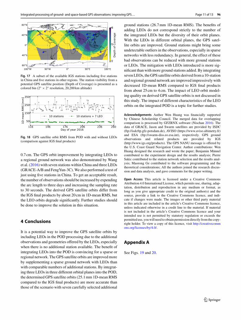
To show the potential benefits of supplementing a region-ally distributed ground network by integrating LEOs, weselected an additional subset of the available IGS stations.Figure 17 represents the network with five stations in Chinaand another five stations in other regions. The figure showsthat about two-thirds of potential GPS satellite positions(2◦ × 2◦ resolution, 20,200km altitude) can be observed byonly two or even fewer stations. The GPS-only and seven-LEO-integrated PODwere performedwith this network. The1D-mean RMS of the GPS satellite orbit differences com-pared to the IGS final products are presented in Fig. 18.Enhanced by seven LEOs, the 1D-mean RMS decreases sig-nificantly from about 25cm to 4cm. Also, the variations ofthe time series are reduced significantly from about 4.3cm to

123

Integrated processing of ground- and space-based GPS observations: improving GPS… Page 11 of 13 96

Fig. 17 A subset of the available IGS stations including five stationsin China and five stations in other regions. The station visibility from apotential GPS satellite position (Depth of Coverage) is presented as acolored bin (2◦ × 2◦ resolution, 20,200km altitude)

Fig. 18 GPS satellite orbit RMS from POD with and without LEOs(comparison against IGS final products)

0.7 cm. The GPS orbit improvement by integrating LEOs toa regional ground network was also demonstrated by Wanget al. (2016) with seven stations within China and three LEOs(GRACE-A/B and FengYun-3C).We also performed a test ofjust using five stations in China. To get an acceptable result,the number of observations should be increased by expendingthe arc length to three days and increasing the sampling rateto 30 seconds. The derived GPS satellite orbits differ fromthe IGS final products by about 20cm in 1D-mean RMS, butthe LEO orbits degrade significantly. Further studies shouldbe done to improve the solution in this situation.

4 Conclusions

It is a potential way to improve the GPS satellite orbits byincluding LEOs in the POD processing due to the additionalobservations and geometries offered by the LEOs, especiallywhen there is no additional station available. The benefit ofintegrating LEOs into the POD is convincing for a sparse orregional network. TheGPS satellite orbits are improvedmoreby supplementing a sparse ground network with LEOs thanwith comparable numbers of additional stations. By integrat-ing three LEOs in three different orbital planes into the POD,the determined GPS satellite orbits (25.1mm 1D-mean RMScompared to the IGS final products) are more accurate thanthose of the scenario with seven carefully selected additional

ground stations (26.7mm 1D-mean RMS). The benefits ofadding LEOs do not correspond strictly to the number ofthe integrated LEOs but the diversity of their orbit planes.With the LEOs in different orbital planes, the GPS satel-lite orbits are improved. Ground stations might bring someundetectable outliers in the observations, especially in sparsenetworks with less redundancy. In general, the effect of thesebad observations can be reduced with more ground stationsor LEOs. The mitigation with LEOs introduced is more sig-nificant thanwithmore ground stations added. By integratingsevenLEOs, theGPSsatellite orbits derived froma10-stationand regional ground network are improved impressively withdecreased 1D-mean RMS compared to IGS final productsfrom about 25cm to 4cm. The impact of LEO orbit model-ing quality on derived GPS satellite orbits is not discussed inthis study. The impact of different characteristics of the LEOorbits on the integrated POD is a topic for further studies.

Acknowledgements Author Wen Huang was financially supportedby Chinese Scholarship Council. The merged data for overlappingcomparison is processed by GFZRNX software (Nischan 2016). Thedata of GRACE, Jason and Swarm satellites are provided by ISDC(ftp://isdcftp.gfz-potsdam.de), AVISO (https://www.aviso.altimetry.fr)and ESA (ftp://swarm-diss.eo.esa.int), respectively. GPS groundobservations and related products are provided by IGS(http://www.igs.org/products). The GPS NANU message is offered bythe U.S. Coast Guard Navigation Center. Author contributions: WenHuang designed the research and wrote the paper; Benjamin Männelcontributed to the experiment design and the results analysis; PierreSakic contributed to the station network selection and the results anal-ysis; Maorong Ge contributed to the software programming and thetheoretical considerations; All the authors joined the research discus-sion and data analysis, and gave comments for the paper writing.

Open Access This article is licensed under a Creative CommonsAttribution 4.0 International License, which permits use, sharing, adap-tation, distribution and reproduction in any medium or format, aslong as you give appropriate credit to the original author(s) and thesource, provide a link to the Creative Commons licence, and indi-cate if changes were made. The images or other third party materialin this article are included in the article’s Creative Commons licence,unless indicated otherwise in a credit line to the material. If materialis not included in the article’s Creative Commons licence and yourintended use is not permitted by statutory regulation or exceeds thepermitted use, youwill need to obtain permission directly from the copy-right holder. To view a copy of this licence, visit http://creativecommons.org/licenses/by/4.0/.

Appendix A

See Figs. 19 and 20.

123

96 Page 12 of 13 W. Huang et al.

Fig. 19 A dense subset of the IGS ground stations with 62 globallydistributed stations

Fig. 20 Statistical results of the GPS satellite orbit differences w.r.t.the IGS final products of 62-station scenario and 26-station+7-LEOscenario. The RMS of orbit differences in the along-track, the cross-track, and the radial directions are computed over epochs and satellitesin each day. The 1D-mean RMS is computed over epochs, satellites,and the three orbital directions

References

Berger C, Biancale R, Barlier F, Ill M (1998) Improvement of theempirical thermospheric model DTM: DTM94: a comparativereview of various temporal variations and prospects in spacegeodesy applications. J Geod 72(3):161–178. https://doi.org/10.1007/s001900050158

Blewitt G (1990) An automatic editing algorithm for GPSdata. Geophys Res Lett 17(3):199–202. https://doi.org/10.1029/GL017I003P00199

Case K, Kruizinga G, Wu S (2002) Grace level 1b data product userhandbook. Technical report, JPL

ChoiKK (2014) Status of core products of the international gnss service.AGU Fall Meeting Abstr 2014:G21A–0426

Dumont J, Rosmorduc V, Picot N, Desai S, Bonekamp H, Figa J, Lil-libridge J, Scharroo R (2009) Ostm/jason-2 products handbook.Technical representative, CNES and EUMETSAT and JPL andNOAA/NESDIS

Dumont J, Rosmorduc V, Carrere L, Picot N, Bronner E, Couhert A,Guillot A, Desai S, Bonekamp H, Figa J et al (2016) Jason-3 prod-ucts handbook. Technical representative, CNES and EUMETSATand JPL and NOAA/NESDIS

Friis-Christensen E, Lühr H, Knudsen D, Haagmans R (2008) Swarm:an earth observation mission investigating geospace. Adv SpaceRes 41(1):210–216. https://doi.org/10.1016/J.ASR.2006.10.008

Geng JH, Shi C, Zhao QL, Ge MR, Liu JN (2008) Integrated adjust-ment of LEO and GPS in precision orbit determination. IntAssoc Geod Symp 132:133–137. https://doi.org/10.1007/978-3-540-74584-6_20

Gutierrez P (2018) Brexit and Galileo - Plenty of rumblings,but Where’s the Beef? https://insidegnss.com/brexit-and-galileo-plenty-of-rumblings-but-wheres-the-beef/, online article of insid-egnss.com

Hackel S, Steigenberger P, Hugentobler U, UhlemannM,MontenbruckO (2015) Galileo orbit determination using combined GNSSand SLR observations. GPS Solut 19(1):15–25. https://doi.org/10.1007/s10291-013-0361-5

Haines B, Bar-Sever Y, Bertiger W, Desai S, Willis P (2004) One-centimeter orbit determination for Jason-1: newGPS-based strate-gies. Mar Geod. https://doi.org/10.1080/01490410490465300

Jäggi A, Hugentobler U, Bock H, Beutler G (2007) Precise orbit deter-mination for GRACE using undifferenced or doubly differencedGPS data. Adv Space Res 39(10):1612–1619. https://doi.org/10.1016/j.asr.2007.03.012

JohnstonG,NeilanR,CraddockA,DachR,MeertensC,RizosC (2018)The international GNSS service 2018 update. In: EGU GeneralAssembly Conference Abstracts, vol 20, p 19675

KönigD (2018)A terrestrial reference frame realised on the observationlevel using a GPS-LEO satellite constellation. J Geod. https://doi.org/10.1007/s00190-018-1121-7

König R, Reigber C, Zhu S (2005) Dynamic model orbits and Earthsystem parameters from combined GPS and LEO data. Adv SpaceRes 36(3):431–437. https://doi.org/10.1016/J.ASR.2005.03.064

Kuang D, Bar-Sever Y, Haines B (2015) Analysis of orbital config-urations for geocenter determination with GPS and low-Earthorbiters. J Geod 89(5):471–481. https://doi.org/10.1007/s00190-015-0792-6

Lambin J, Morrow R, Fu LL, Willis JK, Bonekamp H, LillibridgeJ, Perbos J, Zaouche G, Vaze P, Bannoura W, Parisot F, Thou-venot E, Coutin-Faye S, Lindstrom E, Mignogno M (2010) TheOSTM/Jason-2 mission. Mar Geod 10(1080/01490419):491030

Liu J, Ge M (2003) PANDA software and its preliminary resultof positioning and orbit determination. Wuhan Univ J Nat Sci8(2):603–609. https://doi.org/10.1007/BF02899825

Männel B, Rothacher M (2017) Geocenter variations derived froma combined processing of LEO- and ground-based GPS obser-vations. J Geod 91(8):933–944. https://doi.org/10.1007/s00190-017-0997-y

Marshall JA, Antreasian PG, Rosborough GW, Putney BH (1992)Modeling radiation forces acting on satellites for precision orbitdetermination. Adv Astron Sci 76(pt 1):73–96. https://doi.org/10.2514/3.26408

Ménard Y, Fu LL, Escudier P, Parisot F, Perbos J, Vincent P, DesaiS, Haines B, Kunstmann G (2003) The jason-1 mission specialissue: Jason-1 calibration/validation. Mar Geod 26(3–4):131–146.https://doi.org/10.1080/714044514

123

Integrated processing of ground- and space-based GPS observations: improving GPS… Page 13 of 13 96

Montenbruck O, Gill E (2000) Satellite orbits: models, methods, andapplications, 1st edn. Springer, Berlin. https://doi.org/10.1007/978-3-642-58351-3

Montenbruck O, Hackel S, van den Ijssel J, Arnold D (2018) Reduceddynamic and kinematic precise orbit determination for the Swarmmission from 4 years of GPS tracking. GPS Solut 22(3):79. https://doi.org/10.1007/s10291-018-0746-6

Nischan T (2016)GFZRNX-RINEXGNSS data conversion andmanip-ulation toolbox (Version 1.05). GFZData Services. https://doi.org/10.5880/GFZ.1.1.2016.002

Olsen PEH (2019) Swarm l1b product definition. National Space Insti-tute Technical University of Denmark, Technical report

Otten M, Flohrer C, Springer T, Enderle W (2012) Multi-techniquecombination at observation level with napeos: combining GPS,GLONASS and leo satellites. In: EGU general assembly confer-ence abstracts, vol 14, p 7925

Petit G, Luzum B (2010) IERS conventions (2010). Technical report,Bureau international des poids et mesures sevres (France)

Rebischung P, Griffiths J, Ray J, Schmid R, Collilieux X, GaraytB (2012) IGS08: the IGS realization of ITRF2008. GPS Solut16(4):483–494. https://doi.org/10.1007/s10291-011-0248-2

Reigber C, Schmidt R, Flechtner F, König R, Meyer U, NeumayerKH, Schwintzer P, Zhu SY (2005) An earth gravity field modelcomplete to degree and order 150 from grace: Eigen-grace02s. JGeodyn 39(1):1–10. https://doi.org/10.1016/j.jog.2004.07.001

Sakic P, Männel B, Nischan T (2018) Operational geodetic prod-ucts determination and combination for Galileo. In: EGU generalassembly conference abstracts, vol 20, p 17515

Schmid R, Dach R, CollilieuxX, Jäggi A, SchmitzM,Dilssner F (2016)Absolute IGS antenna phase center model igs08.atx: status andpotential improvements. J Geod 90(4):343–364

Springer T, Beutler G, Rothacher M (1999) A new solar radiation pres-sure model for GPS satellites. GPS Solut 2(3):50–62. https://doi.org/10.1007/PL00012757

Standish EM (1998) JPL planetary and lunar ephemerides,DE405/LE405. Jpl Iom 312F-98-048

Tapley BD, Bettadpur S, Ries JC, Thompson PF, Watkins MM (2004)GRACE measurements of mass variability in the Earth system.Science. https://doi.org/10.1126/science.1099192

Vaze P, Neeck S, BannouraW,Green J,WadeA,MignognoM, ZaoucheG, Couderc V, Thouvenot E, Parisot F (2010) The Jason-3 mis-sion: completing the transition of ocean altimetry from researchto operations. In: Sensors, systems, and next-generation satellitesXIV, International Society for Optics and Photonics, vol 7826, p78260Y

Wang L, Zhang Q, Huang G, Yan X, Qin Z (2016) Combining regionalmonitoring stations with space-based data to determine the MEOsatellite orbit. Acta Geod Cartograph Sin 45(S2):101

WuSC,YunckTP, ThorntonCL (1991)Reduced-dynamic technique forprecise orbit determination of low earth satellites. J Guid ControlDyn 14(1):24–30. https://doi.org/10.2514/3.20600

Yang Y (2018) Introduction to BeiDou-3 navigation satellite system.Presented in IGS workshop October 2018, Wuhan, China

Zhao Q, Wang C, Guo J, Yang G, Liao M, Ma H, Liu J (2017)Enhanced orbit determination for BeiDou satellites with FengYun-3C onboard GNSS data. GPS Solut 21(3):1179–1190. https://doi.org/10.1007/s10291-017-0604-y

Zhao Q, Wang C, Guo J, Wang B, Liu J (2018) Precise orbit and clockdetermination for BeiDou-3 experimental satellites with yaw atti-tude analysis. GPS Solut 22(1):4. https://doi.org/10.1007/s10291-017-0673-y

Zhu S, Reigber C, König R (2004) Integrated adjustment of CHAMP,GRACE, and GPS data. J Geod 78(1–2):103–108. https://doi.org/10.1007/s00190-004-0379-0

ZoulidaM, Pollet A, Coulot D, Perosanz F, Loyer S, Biancale R, Rebis-chung P (2016) Multi-technique combination of space geodesyobservations: impact of the Jason-2 satellite on the GPS satelliteorbits estimation. Adv Space Res 58(7):1376–1389. https://doi.org/10.1016/j.asr.2016.06.019

123