INTEGRATED MEASURES OFSALES, MERCHANDISING, AND DISTRIBUTION

John D.C. Little

M.I.T. Sloan School of Management, Cambridge, MA 02142, U.S.A.

Sloan Working Paper # 3997July 1998

ABSTRACT

Managers track marketing performance with measures of sales, distribution, andmerchandising. These can be calculated at different levels of aggregation with respect togeographic areas, time periods, and products. To be most useful, performance measuresshould have parallel and consistent meanings across the different levels. Starting from thedecomposition of sales into base and incremental volume as provided by data suppliers at theunderlying level of item-store-week, we define a set of performance measures that fit togetherinto a simple model. It is shown that these definitions permit consistent aggregation intoanalogous measures and models at higher levels. An example drawing on Ocean SprayCranberries data illustrates the advantages of the measures for comparing marketingperformance across levels of aggregation.

Key words: scanner data, distribution, merchandising, aggregation

Forthcoming in International Journal of Research in Marketing

1. Introduction

The most frequently quoted numbers from scanner databases are aggregate statistics.Although bar code readers generate huge amounts of detailed data, the sheer quantity ofnumbers forces a search for meaningful summaries. These should express, in simple andsensible ways, what is happening to a brand or product line over broad geographic regionsand time periods. Such aggregates provide top line information about market status andcustomer response and so assist marketers in managing their brands. The same measures areused by senior managers and others, inside and outside a company, who need to stay abreastof market trends.

Summary measures answer such questions as: "How is a brand or product lineperforming overall? Have our products increased in national distribution over the past sixmonths? How effective has our trade support been?" Answers often trigger deeper studiesthat drill down in the databases for further insight. Because the most commonly usednumbers throughout a company are summaries, their construction merits scrutiny forconsistency and clarity.

Marketing scientists have exploited scanner data to study many important phenomena,but have done relatively little with aggregation issues. Exceptions are Christen, Gupta,Porter, Staelin, and Wittink (1997), Gupta, Chintagunta, Kaul, and Wittink (1996), Foekens,Leeflang, and Wittink (1994), Link (1995), and Allenby and Rossi (1991). These authorsinvestigate biases introduced by applying econometric techniques to data that has beenassembled by aggregating from individuals to stores or stores to markets.

The focus here, however, is quite different and not econometric at all. Most of theaggregate information produced by the suppliers of scanner data is more analogous toaccounting reports than to econometric modeling. Relatively simple arithmetic sums andweighted averages serve to accumulate data over products, geographical areas, and timeperiods. The measures commonly produced have the important advantage that they arerelatively transparent in their calculation and interpretation. Such numbers are viewed bythousands of marketers and salespeople daily.

1.1 Scanner Databases.

To give perspective, we briefly sketch the size and scope of the retail store datacollected by the two principal suppliers of scanner data to the consumer packaged goodsindustry in the U.S. and Europe, namely, Information Resources, Inc. (IRI) and theA.C.Nielsen Company (Nielsen). Using the U.S. as a benchmark, the universe of storesbeing monitored consists of approximately 31,000 supermarkets, 38,000 drug stores, 6,400mass merchandise outlets, and 140,000 convenience stores. There are eight million UniversalProduct Codes (UPCs) in IRI's data dictionary, each representing an identifiably differentproduct. Many of them are inactive at any given time, but over 3 million show productmovement during a year. The samples of stores in the IRI and Nielsen services are quitelarge. For example, in mid-1997 IRI's InfoScan contained about 4,515 stores, consisting ofapproximately 3,050 supermarkets, 600 drug stores, 290 mass merchandisers, and 575convenience stores. Typically, the raw data arrives from the stores as weekly sales totals indollars and units by UPC. A store might stock 30,000 UPCs. In addition, stores in the

1

sample are monitored weekly for displays and features. Each store generates from six to tenpermanently retained measures per week per UPC carried. These basic measures areanalyzed in various ways and combined with information from other sources into over 800different measures available to clients.

To swell the data further, information is increasingly collected from all stores in aretail chain, not just a sample. Such census data is replacing samples for many applications.In particular, for a manufacturer's sales force dealing with retail chains, it helps two-waycommunication between manufacturer and retailer when both work from the same, completedata. In 1997 IRI collected information from over 24,000 stores and its online databaseexceeded two terrabytes.

In other countries the number of products, although not quite as large, has a similarorder of magnitude. A chief difference is that the size of the country determines the numberof stores. Different countries also have different mixes of store types and may have differentproduct codes. In Europe products are identified by European Article Numbers (EAN), inJapan by Japanese Article Numbers (JAN).

Individual store data for, say, a half dozen measures over two years by item and weekfor a major category runs into billions of records and is prohibitively time consuming to workwith except for special studies. Therefore, Nielsen and IRI perform a first step of aggregatingdata across stores into markets or other useful groupings before delivery. In the case ofsample data, such aggregation involves projection.

To bring some order into the large number of UPCs, products are partitioned intocategories. Although over 820 categories are in common use and many UPCs are not active,this still leaves many products per category. For example, a large category such as cereals orcarbonated soft drinks would contain several tens of thousands of individual products.Further organization is required. Products within a category are therefore groupedhierarchically, for example, by manufacturer, brand, sub-brand, size, package, and flavor, thescope and order being specified by the client requesting the data. Each level in such ahierarchy is a candidate for aggregation.

1.2 Aggregation

Marketers want aggregations over at least three dimensions: geography, time, andproduct. Projections and aggregations often require weighting store data by the size of thestore. In such cases size is usually measured in terms of a store's all commodity volume(ACV), which would be expressed, for example, in millions of dollars per year. Thisprocedure is standard and will be assumed, although other methods could be used andsometimes are necessary for special purposes. Aggregation over time usually means adding(or averaging) over weeks. We shall argue that this should be done in certain cases where itis not done now. Aggregation over products is a less obvious process and will be a majorconcern of the paper.

Sales. Sales themselves are usually easy to add up, even when they include items ofdifferent sizes. Most manufacturers define a physical unit, such as kilograms or liters, orother "equivalent volume." Equivalent units make different sizes comparable. We assume

2

that this step has been taken for all products being aggregated so that sales of items across aproduct line or category add to meaningful totals. Adding sales across time periods is alsostraightforward.

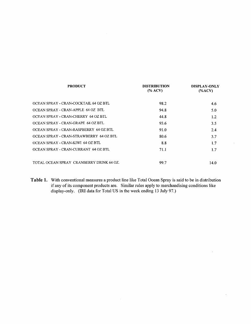
More troublesome, however, are distribution and merchandising. Both IRI's Infoscanservice and Nielsen's Scantrack produce widely disseminated "non-additive" measures fordistribution and merchandising. As an example, Table 1 shows a week's data for a productline, Total Ocean Spray Cranberry Drinks 64 Oz, and eight items that make it up. Shown arethe distribution and display measures for the individual items and, as would commonly bereported, for the line as a whole. The measures are called non-additive because their valuesfor aggregates are not simple sums or averages of their components.

Distribution. Distribution for an individual item is the percentage of stores with non-zero sales of the item, where each store is weighted by its size as measured by all commodityvolume (ACV). Therefore distribution has units of %ACV. In Table 1, for example, 98.2%ACV distribution for Ocean Spray Cran-Cocktail 64 Oz means that this product was sold ina set of stores that constituted 98.2% of the all commodity volume in the geographic areaunder consideration.

Merchandising. Merchandising is a generic name for promotional activity conductedby a store to increase sales. Data companies report four mutually exclusive types ofmerchandising: (1) display only, (2) feature only, (3) display andfeature together, and (4)unsupported price cuts. Several of these can be subdivided further, if desired. Features areadvertisements in newspapers or store flyers. Unsupported price cuts refer to temporary shelfprice reductions in the absence of special display or feature.

For illustrative purposes, consider display-only. Measures of merchandising activitycan be defined analogously to those for distribution. For example, in Table 1, the value of4.6 %ACV with display-only for Ocean Spray Cran-Cocktail 64 Oz means that this producthad a display (but no feature) in a set of stores that represent 4.6% of all commodity volumein the region under consideration.

Questions arise, however, about the rules for aggregating distribution andmerchandising. For example, the display of a product line like Total Ocean Spray CranberryDrink 64 Oz is commonly determined as follows: The line is considered to be on display in astore for the week if any of its component items are on display. Similarly, the product line isin distribution in a store if any of its components are in distribution.

Thus, in Table 1, we see that Total Ocean Spray Cranberry Drink 64 Oz has 99.7%distribution even though one of its individual items is in stores representing only 8.8% ofACV. Similarly, the display-only measure for the aggregate is much larger than any of itsindividual items.

An analogous rule is commonly used for time aggregation. Take, for example, a 12-week period. The 64 ounce bottle of Cran-Grape is said to be on display in a store during theperiod if it was on display during any of the 12 weeks. (Strict enforcement of this definitionrequires excessive computation and so data companies use an approximation, but the resultsare similar.)

3

PRODUCT DISTRIBUTION DISPLAY-ONLY(% ACV) (%ACV)

OCEAN SPRAY - CRAN-COCKTAIL 64 OZ BTL 98.2 4.6

OCEAN SPRAY - CRAN-APPLE 64 OZ BTL 94.8 5.0

OCEAN SPRAY - CRAN-CHERRY 64 OZ BTL 44.8 1.2

OCEAN SPRAY - CRAN-GRAPE 64 OZ BTL 93.6 3.5

OCEAN SPRAY - CRAN-RASPBERRY 64 OZ BTL 91.0 2.4

OCEAN SPRAY - CRAN-STRAWBERRY 64 OZ BTL 80.6 3.7

OCEAN SPRAY - CRAN-KIWI 64 OZ BTL 8.8 1.7

OCEAN SPRAY - CRAN-CURRANT 64 OZ BTL 71.1 1.7

TOTAL OCEAN SPRAY CRANBERRY DRINK 64 OZ. 99.7 14.0

Table 1. With conventional measures a product line like Total Ocean Spray is said to be in distributionif any of its component products are. Similar rules apply to merchandising conditions likedisplay-only. (IRI data for Total US in the week ending 13 July 97.)

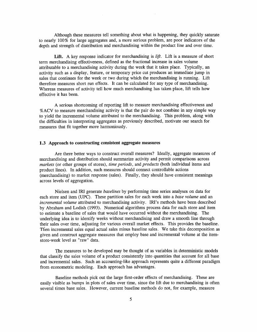
Although these measures tell something about what is happening, they quickly saturateto nearly 100% for large aggregates and, a more serious problem, are poor indicators of thedepth and strength of distribution and merchandising within the product line and over time.

Lift. A key response indicator for merchandising is lift. Lift is a measure of shortterm merchandising effectiveness, defined as the fractional increase in sales volumeattributable to a merchandising activity during the week that it takes place. Typically, anactivity such as a display, feature, or temporary price cut produces an immediate jump insales that continues for the week or two during which the merchandising is running. Lifttherefore measures short run effects. It can be calculated for any type of merchandising.Whereas measures of activity tell how much merchandising has taken place, lift tells howeffective it has been.

A serious shortcoming of reporting lift to measure merchandising effectiveness and%ACV to measure merchandising activity is that the pair do not combine in any simple wayto yield the incremental volume attributed to the merchandising. This problem, along withthe difficulties in interpreting aggregates as previously described, motivate our search formeasures that fit together more harmoniously.

1.3 Approach to constructing consistent aggregate measures

Are there better ways to construct overall measures? Ideally, aggregate measures ofmerchandising and distribution should summarize activity and permit comparisons acrossmarkets (or other groups of stores), time periods, and products (both individual items andproduct lines). In addition, such measures should connect controllable actions(merchandising) to market response (sales). Finally, they should have consistent meaningsacross levels of aggregation.

Nielsen and IRI generate baselines by performing time series analyses on data foreach store and item (UPC). These partition sales for each week into a base volume and anincremental volume attributed to merchandising activity. IRI's methods have been describedby Abraham and Lodish (1993). Numerical algorithms process data for each store and itemto estimate a baseline of sales that would have occurred without the merchandising. Theunderlying idea is to identify weeks without merchandising and draw a smooth line throughtheir sales over time, adjusting for various overall market effects. This provides the baseline.Tlhen incremental sales equal actual sales minus baseline sales. We take this decomposition asgiven and construct aggregate measures that employ base and incremental volume at the item-store-week level as "raw" data.

The measures to be developed may be thought of as variables in deterministic modelsthat classify the sales volume of a product consistently into quantities that account for all baseand incremental sales. Such an accounting-like approach represents quite a different paradigmfrom econometric modeling. Each approach has advantages.

Baseline methods pick out the large first-order effects of merchandising. These areeasily visible as bumps in plots of sales over time, since the lift due to merchandising is oftenseveral times base sales. However, current baseline methods do not, for example, measure

5

the complex influences that the merchandising of one product may have on related products.Such effects can often be estimated by econometric modeling in studies designed for thepurpose. Econometric techniques also permit the examination of other issues not addressed instandard IRI and Nielsen measures. Foekens, Leeflang, and Wittink (1994) present a type ofmultiplicative model that is frequently employed. Such models can often yield valuableinformation about complex market responses.

Econometric and baseline approaches have different characteristics. An econometricmodel will ordinarily estimate parameter values from many pieces of data. For example, asingle display effectiveness parameter would normally be estimated from data containing manymerchandising events. In contrast, Nielsen and IRI baseline methods estimate a separatedisplay effectiveness for each event. Since events differ in their execution, the individualevent analysis often provides important information. Furthermore many marketers like tohave values of sales and incremental sales that add up to total actual sales in an accounting-like way. Econometric models yield estimates that ordinarily do not do this. On the otherhand, econometric models are good at measuring more subtle phenomena than can bediscerned by the current baseline approaches. Marketers often want both kinds of informationand so use both types of analysis.

The focus here is on improving the consistency and meaningfulness of accounting-likemeasures of sales, distribution, and merchandising and so takes as given the time-seriesdecomposition into base and incremental volume. If methods are devised that produce bettercalculations of these inputs, they can be substituted in what follows.

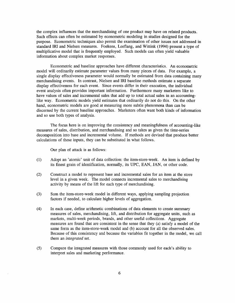
Our plan of attack is as follows:

(1) Adopt an 'atomic' unit of data collection: the item-store-week. An item is defined byits finest grain of identification, normally, its UPC, EAN, JAN, or other code.

(2) Construct a model to represent base and incremental sales for an item at the storelevel in a given week. The model connects incremental sales to merchandisingactivity by means of the lift for each type of merchandising.

(3) Sum the item-store-week model in different ways, applying sampling projectionfactors if needed, to calculate higher levels of aggregation.

(4) In each case, define arithmetic combinations of data elements to create summarymeasures of sales, merchandising, lift, and distribution for aggregate units, such asmarkets, multi-week periods, brands, and other useful collections. Aggregatemeasures are found that are consistent in the sense that they (a) satisfy a model of thesame form as the item-store-week model and (b) account for all the observed sales.Because of this consistency and because the variables fit together in the model, we callthem an integrated set.

(5) Compare the integrated measures with those commonly used for each's ability tointerpret sales and marketing performance.

6

2. Analytic Development

The simple ideas that we use repeatedly are: (1) sales volume = base volume +incremental volume, (2) incremental volume = (base volume) x (merchandising activity) x(lift due to merchandising activity), and (3) base volume = (base volume per unit ofdistribution) x (distribution).

2.1 Store level data and model

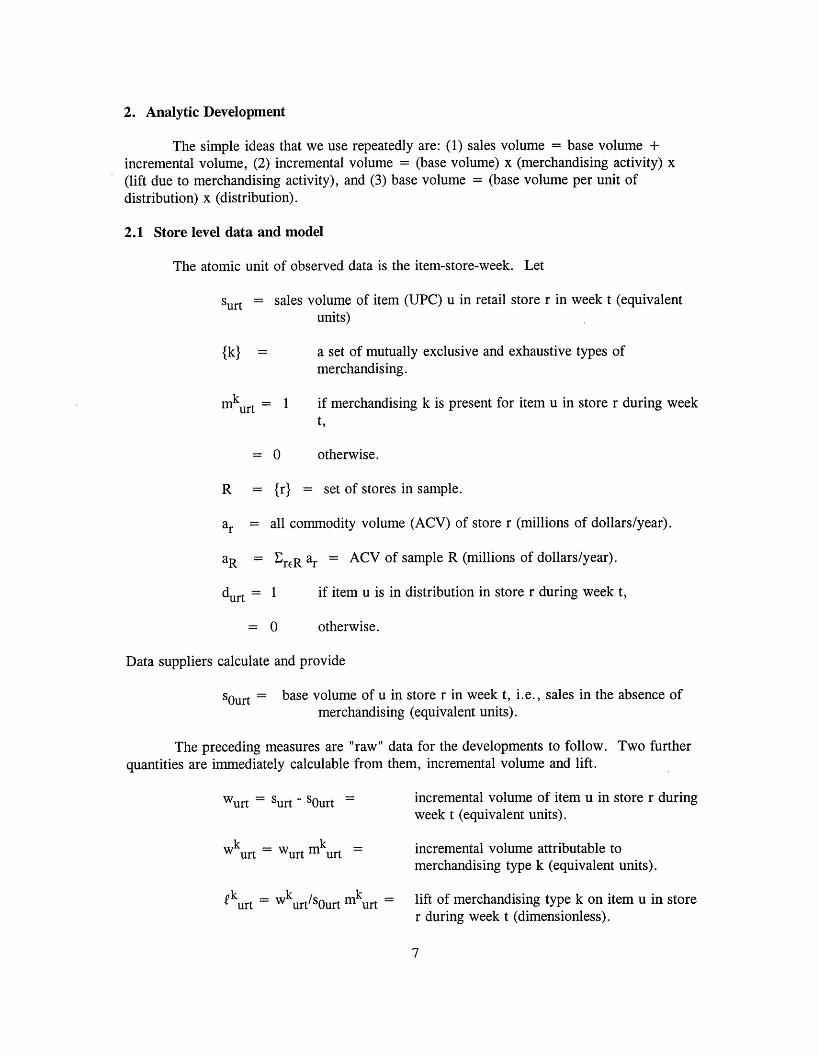
The atomic unit of observed data is the item-store-week. Let

surt = sales volume of item (UPC) u in retail store r in week t (equivalentunits)

{k} a set of mutually exclusive and exhaustive types ofmerchandising.

mkurt = 1 if merchandising k is present for item u in store r during week

= 0 otherwise.

R = {r} = set of stores in sample.

ar = all commodity volume (ACV) of store r (millions of dollars/year).

aR = reR ar = ACV of sample R (millions of dollars/year).

durt = 1

= 0

if item u is in distribution in store r during week t,

otherwise.

Data suppliers calculate and provide

SOurt = base volume of u in store r in week t, i.e., sales in the absence ofmerchandising (equivalent units).

The preceding measures are "raw" data for the developments to follow. Two furtherquantities are immediately calculable from them, incremental volume and lift.

Wurt = Surt- SOurt =

wkrt = Wurt mkurt

ekurt = wkurt/sOurt mkurt =

incremental volume of item u in store r duringweek t (equivalent units).

incremental volume attributable tomerchandising type k (equivalent units).

lift of merchandising type k on item u in storer during week t (dimensionless).

7

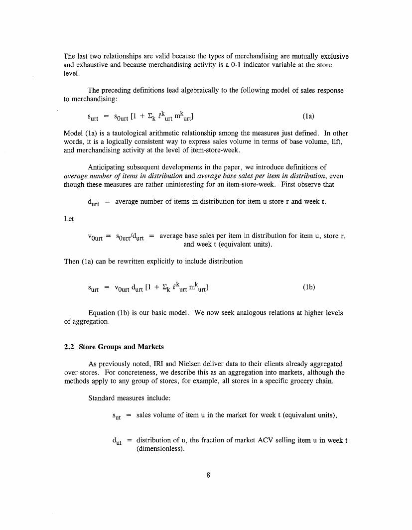
The last two relationships are valid because the types of merchandising are mutually exclusiveand exhaustive and because merchandising activity is a 0-1 indicator variable at the storelevel.

The preceding definitions lead algebraically to the following model of sales responseto merchandising:

Surt = SOurt [1 + Sk ekurt mkurt] (la)

Model (la) is a tautological arithmetic relationship among the measures just defined. In otherwords, it is a logically consistent way to express sales volume in terms of base volume, lift,and merchandising activity at the level of item-store-week.

Anticipating subsequent developments in the paper, we introduce definitions ofaverage number of items in distribution and average base sales per item in distribution, eventhough these measures are rather uninteresting for an item-store-week. First observe that

durt = average number of items in distribution for item u store r and week t.

Let

VOurt = Sourt/durt = average base sales per item in distribution for item u, store r,and week t (equivalent units).

Then (la) can be rewritten explicitly to include distribution

Surt = V0Ourt durt [1 + k fkurt mkurt] (lb)

Equation (lb) is our basic model. We now seek analogous relations at higher levelsof aggregation.

2.2 Store Groups and Markets

As previously noted, IRI and Nielsen deliver data to their clients already aggregatedover stores. For concreteness, we describe this as an aggregation into markets, although themethods apply to any group of stores, for example, all stores in a specific grocery chain.

Standard measures include:

sut = sales volume of item u in the market for week t (equivalent units),

dut = distribution of u, the fraction of market ACV selling item u in week t(dimensionless).

8

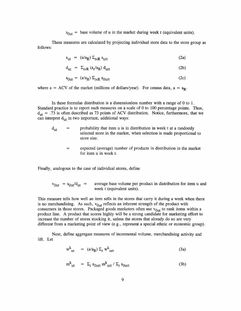
sOut = base volume of u in the market during week t (equivalent units).

These measures are calculated by projecting individual store data to the store group asfollows:

Sut = (a/aR) EreR Surt (2a)

dut = EreR (ar/aR) durt (2b)

sOut = (a/aR) EreR SOurt (2c)

where a = ACV of the market (millions of dollars/year). For census data, a = aR.

In these formulas distribution is a dimensionless number with a range of 0 to 1.Standard practice is to report such measures on a scale of 0 to 100 percentage points. Thus,dUt = .73 is often described as 73 points of ACV distribution. Notice, furthermore, that wecan interpret dut in two important, additional ways:

dut = probability that item u is in distribution in week t at a randomlyselected store in the market, when selection is made proportional tostore size.

expected (average) number of products in distribution in the marketfor item u in week t.

Finally, analogous to the case of individual stores, define

VOut = sut/dut = average base volume per product in distribution for item u andweek t (equivalent units).

This measure tells how well an item sells in the stores that carry it during a week when thereis no merchandising. As such, vut reflects an inherent strength of the product withconsumers in those stores. Packaged goods marketers often use vou t to rank items within aproduct line. A product that scores highly will be a strong candidate for marketing effort toincrease the number of stores stocking it, unless the stores that already do so are verydifferent from a marketing point of view (e.g., represent a special ethnic or economic group).

Next, define aggregate measures of incremental volume, merchandising activity andlift. Let

wkut = (a/aR) Er wkurt (3a)

mkut = ur S0u rt m rSurt (3b)

9

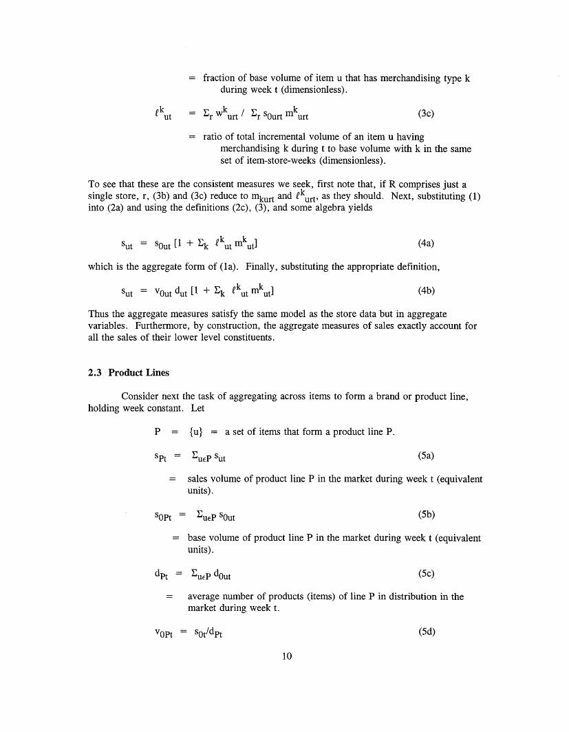
= fraction of base volume of item u that has merchandising type kduring week t (dimensionless).

ek kkut = Er wkurt / 'r sOur t (3c)

= ratio of total incremental volume of an item u havingmerchandising k during t to base volume with k in the sameset of item-store-weeks (dimensionless).

To see that these are the consistent measures we seek, first note that, if R comprises just asingle store, r, (3b) and (3c) reduce to mkurt and Ek urt, as they should. Next, substituting (1)into (2a) and using the definitions (2c), (3), and some algebra yields

Sut = S0Out [1 + Sk lkut mkut] (4a)

which is the aggregate form of (la). Finally, substituting the appropriate definition,

Sut = VOut dut [1 + k ekut mkut] (4b)

Thus the aggregate measures satisfy the same model as the store data but in aggregatevariables. Furthermore, by construction, the aggregate measures of sales exactly account forall the sales of their lower level constituents.

2.3 Product Lines

Consider next the task of aggregating across items to form a brand or product line,holding week constant. Let

P = {u} = a set of items that form a product line P.

SPt = ueP Sut (5a)

= sales volume of product line P in the market during week t (equivalentunits).

SOPt = EueP SOut (5b)

= base volume of product line P in the market during week t (equivalentunits).

dpt = ueP dOut (5c)

= average number of products (items) of line P in distribution in themarket during week t.

Vopt = Sot/dpt (5d)

10

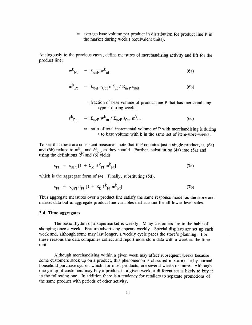
= average base volume per product in distribution for product line P inthe market during week t (equivalent units).

Analogously to the previous cases, define measures of merchandising activity and lift for theproduct line:

wkpt = ueP wkut (6a)

mkPt = ueP Sout mkt / EuEP ut (6b)

= fraction of base volume of product line P that has merchandisingtype k during week t

fkpt = ueP wkut / ueP S0ut (6c)

= ratio of total incremental volume of P with merchandising k duringt to base volume with k in the same set of item-store-weeks.

To see that these are consistent measures, note that if P contains just a single product, u, (6a)and (6b) reduce to mk ut and kut, as they should. Further, substituting (4a) into (5a) andusing the definitions (5) and (6) yields

Spt = sOpt [1 + k ekpt mkpt] (7a)

which is the aggregate form of (4). Finally, substituting (5d),

spt = vOpt dpt [1 + k fkpt mkpt] (7b)

Thus aggregate measures over a product line satisfy the same response model as the store andmarket data but in aggregate product line variables that account for all lower level sales.

2.4 Time aggregates

The basic rhythm of a supermarket is weekly. Many customers are in the habit ofshopping once a week. Feature advertising appears weekly. Special displays are set up eachweek and, although some may last longer, a weekly cycle paces the store's planning. Forthese reasons the data companies collect and report most store data with a week as the timeunit.

Although merchandising within a given week may affect subsequent weeks becausesome customers stock up on a product, this phenomenon is obscured in store data by normalhousehold purchase cycles, which, for most products, are several weeks or more. Althoughone group of customers may buy a product in a given week, a different set is likely to buy itin the following one. In addition there is a tendency for retailers to separate promotions ofthe same product with periods of other activity.

11

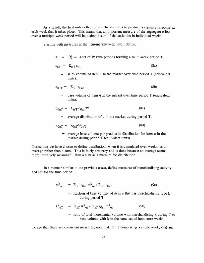
As a result, the first order effect of merchandising is to produce a separate response ineach week that it takes place. This means that an important measure of the aggregate effectover a multiple week period will be a simple sum of the activities in individual weeks.

Starting with measures at the item-market-week level, define:

T = {t} = a set of W time periods forming a multi-week period T.

SuT = EteT Sut (8a)

= sales volume of item u in the market over time period T (equivalentunits).

SOuT = ZteT SOut (8b)

= base volume of item u in the market over time period T (equivalentunits).

dOuT = 1teT dOut/W (8c)

= average distribution of u in the market during period T.

VOuT = SOuT/dOuT (8d)

= average base volume per product in distribution for item u in themarket during period T (equivalent units).

Notice that we have chosen to define distribution, when it is cumulated over weeks, as anaverage rather than a sum. This is fairly arbitrary and is done because an average seemsmore intuitively meaningful than a sum as a measure for distribution.

In a manner similar to the previous cases, define measures of merchandising activityand lift for the time period:

mkUT = EteT S0ut mkut / EteT SOut (9a)

= fraction of base volume of item u that has merchandising type kduring period T

fkuT = teT wkut / gteT SOut mkut (9b)

= ratio of total incremental volume with merchandising k during T tobase volume with k in the same set of item-store-weeks.

To see that these are consistent measures, note that, for T comprising a single week, (9a) and

12

(9b) reduce to mkut and kut, as desired. Further, substituting (4a) into (8a) and using thedefinitions (8) and (9) yields

SuT = sOuT [1 + Sk fkuT mkuT] (10a)

which is the aggregate form of (4a). Finally, substituting (8d),

SuT = VOuT duT [1 + k kuT mkuT] (10b)

Thus the aggregate measures for multi-week period T satisfy the same model as the store andmarket data but in multi-week variables that account for all single week sales.

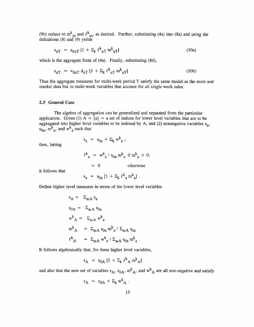
2.5 General Case

The algebra of aggregation can be generalized and separated from the particularapplication. Given (1) A = {a} = a set of indices for lower level variables that are to beaggregated into higher level variables to be indexed by A, and (2) nonnegative variables s a ,s0a, mka, and wka such that

Sa = SOa + k wa;then, letting

ka = wka / SOa mka if mka > 0;

= 0 otherwiseit follows that

a = SOa [1 + k fk a m k a] .

Define higher level measures in terms of the lower level variables

SA = ;aeA Sa

SOA = aeA SOa

wkA = aeA wk a

mkA = EaeA SOa mka / aeA SOa

A = aeA w ka / EaeA SOa mka -

It follows algebraically that, for these higher level variables,

SA = SOA [1 + lk kA m kA]

and also that the new set of variables sA, s0A, mkA, and wkA are all non-negative and satisfy

SA = SOA + kwk A

13

This last expression shows that the aggregation process is recursive. Therefore, wecan take any level of product aggregation and create a higher one in a consistent manner. Forexample, a set of product lines can be aggregated into a product "portfolio". Furthermore,having aggregated on one dimension, we can aggregate on another and obtain parallelformulas.

3. Empirical comparisons

Tables 2 and 3 compare integrated measures with conventional ones for the OceanSpray products considered previously. Data is for Total US Food sales in the period ending13 July 1997, as reported by IRI.

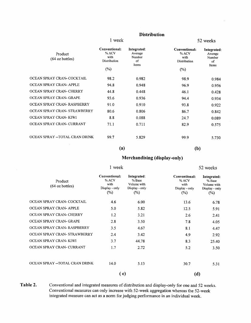
Distribution. Tables 2a and 2b compare distribution measures for one-week and 52-week periods.

One-week. Our integrated measure is average number of items in distribution, whichis to be compared with the conventional %ACV with distribution. For an individual item, thetwo are identical except for the decimal point. They are just two interpretations of the samenumber, as may be seen in Table 2a. The difference comes at aggregation, exemplified hereby the product line, Total Cranberry Drinks. The integrated average number of items indistribution is simply the sum over the items and equals 5.83. This seems like a usefulsummary of how widely available in stores are the 8 items of the product line. Such ameasure can be watched from week to week as marketing tactics unfold.

The conventional, non-additive measure, which considers the product line to bepresent whenever any of its items are present, has the value 99.7%. This is a high value,crowding 100%, that does not seem to add much information not already contained in theindividual items, since one them has 98.2% distribution. Of course, the conventional measurewill sometimes be interesting and useful since it describes a different aspect of the data.However, if a choice must be made between the two measures in the interests of brevity, theintegrated version seems to tell more. The conventional measure could remain in thebackground, obtainable by drill down.

52-weeks. Time aggregation illustrates the utility of the integrated measures asnorms. We can make such statements as, "In the current week, the average numbers of itemsin distribution for Cran Cherry and Cran Currant are ahead of their 52-week values but CranStrawberry is behind. Furthermore, the product line, Total Cranberry Drinks, is ahead." Bycontrast, the conventional measure, %ACV with distribution, because of the way it is defined,can only increase with aggregation and so cannot perform the analogous role. For example,the %ACV with distribution of Total Cranberry Drinks for the current week is 99.7%, whichis behind (rather than ahead of) the 52-week value of 99.9%. These numbers also show howsaturation toward 100% reduces the meaningfulness of the conventional measure.

14

Distribution1 week 52 weeks

Conventional: Integrated: Conventional: Integrated:Product % ACV Average % ACV Average

with Number with Number(64 oz bottles) Distribution of Distribution ofItems Items

(%) (%)

OCEAN SPRAY CRAN- COCKTAIL 98.2 0.982 98.9 0.984

OCEAN SPRAY CRAN- APPLE 94.8 0.948 96.9 0.956

OCEAN SPRAY CRAN- CHERRY 44.8 0.448 46.1 0.428

OCEAN SPRAY CRAN- GRAPE 93.6 0.936 94.4 0.934

OCEAN SPRAY CRAN- RASPBERRY 91.0 0.910 93.8 0.922

OCEAN SPRAY CRAN- STRAWBERRY 80.6 0.806 86.7 0.842

OCEAN SPRAY CRAN- KIWI 8.8 0.088 24.7 0.089

OCEAN SPRAY CRAN- CURRANT 71.1 0.711 82.9 0.575

OCEAN SPRAY --TOTAL CRAN DRINK 99.7 5.829 99.9 5.730

(a) (b)

Merchandising (display-only)

1 week 52 weeks

Conventional: Integrated: Conventional: Integrated:Product % ACV % Base % ACV % Base

with Volume with with Volume withDisplay - only Display - only Display -only Display -only

(%) (%) (%) (%)

OCEAN SPRAY CRAN- COCKTAIL 4.6 6.00 13.6 6.78

OCEAN SPRAY CRAN- APPLE 5.0 5.82 12.5 5.91

OCEAN SPRAY CRAN- CHERRY 1.2 3.21 2.6 2.41

OCEAN SPRAY CRAN- GRAPE 2.8 3.50 7.8 4.05

OCEAN SPRAY CRAN- RASPBERRY 3.5 4.67 8.1 4.47

OCEAN SPRAY CRAN- STRAWBERRY 2.4 3.42 4.9 2.92

OCEAN SPRAY CRAN- KIWI 3.7 44.78 8.3 25.40

OCEAN SPRAY CRAN- CURRANT 1.7 2.72 5.2 3.50

OCEAN SPRAY --TOTAL CRAN DRINK 14.0 5.13 30.7 5.31

(c) (d)

Table 2. Conventional and integrated measures of distribution and display-only for one and 52 weeks.Conventional measures can only increase with 52-week aggregation whereas the 52-weekintegrated measure can act as a norm for judging performance in an individual week.

Merchandising. The integrated measure for merchandising activity is quite differentfrom the conventional one. Its construction achieves consistency and also makes it a relevantnorm across levels of aggregation. Tables 2c and 2d show one-week and 52-weekcomparisons.

One-week. Looking first at the conventional measure, %ACV with display-only, forthe product line, Total Cranberry Drink, we find its value to be 14.0%. This is several timesthat for any individual item. Therefore, 14.0% does not provide a norm against which theindividual items can be judged. Neither is it related in any simple way to the incrementalsales generated by display-only conditions. In contrast, the integrated measure, % of basevolume with display-only, has a value 5.13% for the product line. This provides a referencepoint for comparing the performance of the individual items. For example, only 3.50% ofthe base volume of Cran Grape has display-only during this week. Furthermore, because ofthe way 5.13 % for the product line is constructed, it combines with other data in a consistentway to generate the total incremental sales attributed to display-only.

52-week. A similar situation holds for the 52-week time aggregate. The conventionalaggregate neither provides a standard for single week performance nor tells how display-onlyworked to generate extra sales for the item. As an illustration, the 52-week value for Cran-Cocktail is 13.6% for the conventional measure. Although this may be compared with itssingle week value of 4.6%, the comparison seems less useful than the corresponding one forthe integrated measure. In the latter case, the 52-week value of 6.78% can act as a standardand we see that the latest single week value of 6.00% is noticeably below the 52-weekaverage. Furthermore, the integrated measure combines with lift factors and base volume toplay back the incremental sales attributed to display-only conditions.

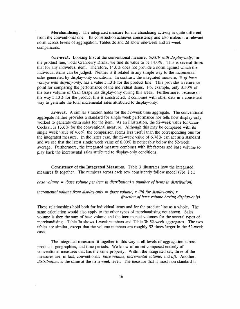
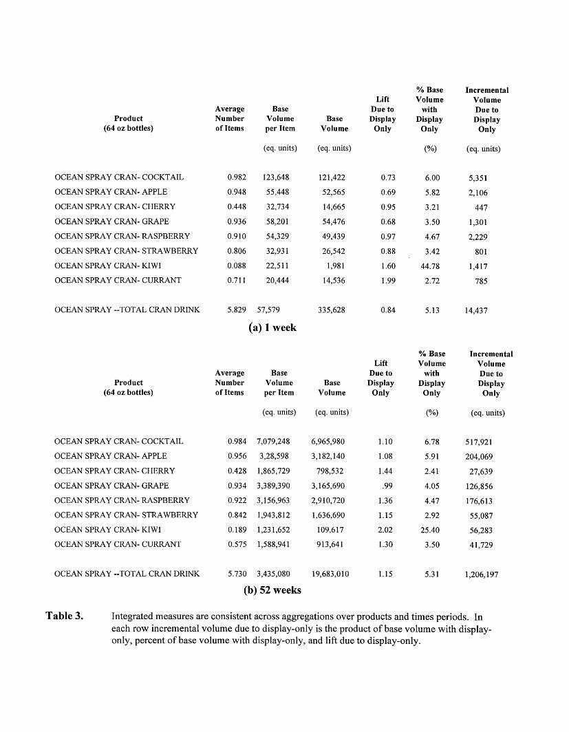
Consistency of the Integrated Measures. Table 3 illustrates how the integratedmeasures fit together. The numbers across each row consistently follow model (7b), i.e.:

base volume = (base volume per item in distribution) x (number of items in distribution)

incremental volume from display-only = (base volume) x (lift for display-only) x(fraction of base volume having display-only)

These relationships hold both for individual items and for the product line as a whole. Thesame calculation would also apply to the other types of merchandising not shown. Salesvolume is then the sum of base volume and the incremental volumes for the several types ofmerchandising. Table 3a shows 1-week numbers and Table 3b 52-week aggregates. The twotables are similar, except that the volume numbers are roughly 52 times larger in the 52-weekcase.

The integrated measures fit together in this way at all levels of aggregation acrossproducts, geographies, and time periods. We know of no set composed entirely ofconventional measures that has the same property. Within the integrated set, three of themeasures are, in fact, conventional: base volume, incremental volume, and lift. Another,distribution, is the same at the item-week level. The measure that is most non-standard is

16

% Base IncrementalLift Volume Volume

Average Base Due to with Due toProduct Number Volume Base Display Display Display

(64 oz bottles) of Items per Item Volume Only Only Only

(eq. units) (eq. units) (0%) (eq. units)

OCEAN SPRAY CRAN- COCKTAIL 0.982 123,648 121,422 0.73 6.00 5,351

OCEAN SPRAY CRAN- APPLE 0.948 55,448 52,565 0.69 5.82 2,106

OCEAN SPRAY CRAN- CHERRY 0.448 32,734 14,665 0.95 3.21 447

OCEAN SPRAY CRAN- GRAPE 0.936 58,201 54,476 0.68 3.50 1,301

OCEAN SPRAY CRAN- RASPBERRY 0.910 54,329 49,439 0.97 4.67 2,229

OCEAN SPRAY CRAN- STRAWBERRY 0.806 32,931 26,542 0.88 3.42 801

OCEAN SPRAY CRAN- KIWI 0.088 22,511 1,981 1.60 44.78 1,417

OCEAN SPRAY CRAN- CURRANT 0.711 20,444 14,536 1.99 2.72 785

OCEAN SPRAY --TOTAL CRAN DRINK 5.829 57,579 335,628 0.84 5.13 14,437

(a) 1 week

% Base IncrementalLift Volume Volume

Average Base Due to with Due toProduct Number Volume Base Display Display Display

(64 oz bottles) of Items per Item Volume Only Only Only

(eq. units) (eq. units) (0%) (eq. units)

OCEAN SPRAY CRAN- COCKTAIL 0.984 7,079,248 6,965,980 1.10 6.78 517,921

OCEAN SPRAY CRAN- APPLE 0.956 3,28,598 3,182,140 1.08 5.91 204,069

OCEAN SPRAY CRAN- CHERRY 0.428 1,865,729 798,532 1.44 2.41 27,639

OCEAN SPRAY CRAN- GRAPE 0.934 3,389,390 3,165,690 .99 4.05 126,856

OCEAN SPRAY CRAN- RASPBERRY 0.922 3,156,963 2,910,720 1.36 4.47 176,613

OCEAN SPRAY CRAN- STRAWBERRY 0.842 1,943,812 1,636,690 1.15 2.92 55,087

OCEAN SPRAY CRAN- KIWI 0.189 1,231,652 109,617 2.02 25.40 56,283

OCEAN SPRAY CRAN- CURRANT 0.575 1,588,941 913,641 1.30 3.50 41,729

OCEAN SPRAY --TOTAL CRAN DRINK 5.730 3,435,080 19,683,010 1.15 5.31 1,206,197

(b) 52 weeks

Table 3. Integrated measures are consistent across aggregations over products and times periods. Ineach row incremental volume due to display-only is the product of base volume with display-only, percent of base volume with display-only, and lift due to display-only.

merchandising activity. This variable knits the others together and permits the simpledecomposition of sales volume into its components at all levels of aggregation.

4. Conclusions

In order to understand and discuss market performance, managers and analysts needsummary measures of sales, distribution and merchandising. Aggregation must be possibleover time, geographic areas, and products. Good measures of merchandising and distributionare ones that are intuitively meaningful and fit together in consistent ways.

We have presented a class of integrated measures that start with information routinelyprovided by data suppliers: the decomposition of sales into base and incremental volume, asattributed to mutually exclusive and exhaustive types of merchandising. The decomposition isexpressed in a deterministic, accounting-like model at the item-store-week level. Each of itsvariables is then aggregated analytically to store groups, product lines, and multi-weekperiods. The model retains its algebraic form at each level of aggregation.

The advantages of the integrated measures are (1) interpretability: in certain instancesthe integrated measures seem more meaningful than conventional ones, (2) utility as norms:higher levels of aggregation provide reference values for judging performance at lower levels,(3) transparency: a simple mental model of how the measures fit together is the actual modeland works consistently at all levels of aggregation, and (4) extensibility: new aggregationsover products, store groups, and time periods can be created analogously without difficulty.

It is not suggested that the underlying model captures all merchandising issues ofinterest and, in fact, examples of missing phenomena have been cited. Differences in themeasures show up across all dimensions, since individual stores and items respond in differentways. Marketers will interpret these differences in light of their knowledge about eventstaking place in the market and will draw inferences about the effectiveness of their programs.Differences and anomalies will trigger further analysis. Thus aggregate measures will oftenbe the starting point for drilling deeper into the immense detail offered by scanner data andwill stimulate other types of statistical studies.

ACKNOWLEDGEMENT

The author thanks Gordon Armstrong and Eugenie Murray-Brown of Ocean SprayCranberries, Inc. for data, helpful discussions, and good suggestions.

18

REFERENCES

Abraham, M.M. and L.M. Lodish (1993), "An implemented system for improving promotionproductivity using store scanner data," Marketing Science, 12, 248-269.

Allenby, G.M. and P.E. Rossi (1991), "There is no aggregation bias: why macro logit modelswork," Journal of Business and Economic Statistics, 9, 1-11.

Christen, M., S. Gupta, J.C. Porter, R. Staelin, and D.R. Wittink (1997), "Using market-level data to understand promotion effects in a nonlinear model," Journal ofMarketing Research, 34, 322-346.

Foekens, E.W., P.S.H. Leeflang, and D.R. Wittink (1994), "A comparison and explorationof the forecasting accuracy of nonlinear models at different levels of aggregation,"International Journal of Forecasting, 10, 245-261.

Gupta, S., P. Chintagunta, A. Kaul, and D.R. Wittink (1996), "Do household scanner panelsprovide representative inferences from brand choices: a comparison with store data,"Journal of Marketing Research, 33, 383-398.

IRI (1997), InfoScan Measure Selection Guide, Information Resources, Inc., Chicago.

Link, R. (1995), "Are aggregate scanner data models biased?" Journal of AdvertisingResearch, 35, RC8-12, (Sept-Oct).

19