Automatica 45 (2009) 601–610

Contents lists available at ScienceDirect

Automatica

journal homepage: www.elsevier.com/locate/automatica

Integrated marketing communications in markets with uncertaintyand competitionI

Ashutosh Prasad, Suresh P. Sethi ∗The University of Texas at Dallas, Richardson, TX 75080, USA

a r t i c l e i n f o

Article history:Received 27 November 2007Received in revised form30 April 2008Accepted 12 September 2008Available online 19 December 2008

Keywords:AdvertisingDynamicsBudgetingIntegrated Marketing CommunicationsUncertaintyOptimization

a b s t r a c t

Firms frequently utilize multiple communications instruments as part of their marketing campaign.Interactions between these instruments suggest that firms should apply Integrated MarketingCommunications (IMC) to benefit from the synergies. We review different IMC models and then presenta stochastic IMC model for which explicit closed-loop solutions of the optimal advertising and marketshare are obtained. This enables us to understand the role of firm and market parameters such assynergy on the optimal advertising budget and allocation. For the proposed and existing IMC models,we show that the budget and allocation decisions can be made independently, greatly simplifying theimplementation of IMC.We also show that there is an optimal long-runmarket share that the firm shouldtry to maintain through appropriate use of IMC. Finally, the model and results are generalized to multiple(>2) instruments and multiple competitors.

© 2008 Elsevier Ltd. All rights reserved.

1. Introduction

Firms frequently utilize multiple communications instruments,for example, advertising through multiple media outlets such asTV and print (Jagpal, 1981; Naik & Raman, 2003), concurrentadvertising and promotion (Naik, Raman, & Winer, 2005), andconcurrent advertising and detailing (Chintagunta & Vilcassim,1994; Fruchter & Kalish, 1998; Gatignon & Hanssens, 1987;Gopalakrishna & Chatterjee, 1992). Empirical research has shownthat the effects of these instruments are not independent of eachother. For example, Naik and Raman (2003) report strong supportfor a positive interaction between print and television advertisingon the sales of Dockers Khaki pants.Gopalakrishna and Chatterjee(1992) estimate the interaction of advertising and personal sellingusing data from an electric cables firm and also find a significantpositive effect.Interaction between the instruments of the communications

mix targeted at the same market segments creates synergy —an increase in the effectiveness of each instrument due to thepresence of the other instruments. In other words, the combined

I This paper was not presented at any IFAC meeting. This paper wasrecommended for publication in revised form by Associate Editor Pirooz Vakiliunder the direction of Editor Berç Rüstem.∗ Corresponding author. Tel.: +1 972 883 6245; fax: +1 972 883 5905.E-mail addresses: aprasad@utdallas.edu (A. Prasad), sethi@utdallas.edu

(S.P. Sethi).

0005-1098/$ – see front matter© 2008 Elsevier Ltd. All rights reserved.doi:10.1016/j.automatica.2008.09.018

effect of a communications mix is greater than the sum of theparts (Naik & Raman, 2003). The presence of synergy shouldideally lead firms to use Integrated Marketing Communications(IMC) (Schultz, 1993). IMC can be defined as the strategy ofcoordinating advertising, personal selling, sales promotion, publicrelations, and other promotional activities, with the goal ofproviding clarity, consistency, and maximum communicationsimpact (Schultz, 1993). Practically, a company might place all itsmedia decisions under one agency to allow for coordination andconsistency between brand messages.From a budgetary standpoint, IMC requires not only determin-

ing the total communications budget but also the allocation of thebudget among different instruments, including the different me-dia or the vehicleswithinmedia. For example, a salespersonwhosecompany and products are well known is likely to get a better re-sponse. A firm may spend too little on advertising if this interac-tion effect is ignored. Absent IMC, not just over-advertising (Aaker& Carman, 1982) but also wrong allocation of the communicationsmix could take place (Gopalakrishna & Chatterjee, 1992). Researchshows that proper allocation of advertising acrossmedia and prod-ucts can have a bigger impact on profit than the level of the total adbudget (Doyle & Saunders, 1990). Thus, the research issueswe con-sider are to determine optimal IMC budgeting over time, the opti-mal dynamic allocation to different communications instruments,and the dependence of these decisions on firm andmarket charac-teristics.Despite the importance of IMC, analytical study has only

recently begun to take off, because the interaction effects and

602 A. Prasad, S.P. Sethi / Automatica 45 (2009) 601–610

dynamics tend to make these models difficult to analyze. Inthis paper we propose an IMC model where the firm makestwo advertising spending decisions that are synergistic. Themodel is tractable even under random disturbances. We provideexplicit, closed-loop solutions of the optimal advertising spendingdecisions andmarket share. Comparative statics are presented. Theanalysis leads to a discussion of the impact of synergies on thetotal advertising budget and allocation among the instruments.Part confirms existing results and part provides new answers. Wefind that there is an optimal, long-run market share that the firmshould try to maintain and it should reduce deviations from thiscaused by share decay and randomness through appropriate useof IMC.We then extend the model to multiple (>2) instruments and

show that the insights are unaffected. A general result is obtainedthat encompasses many IMC models in the literature, showingthat allocation and budgeting decisions can be made separately.This result simplifies the application of IMC effects and enables usto extend the analysis to the situation with multiple competitorswhere the competing firms adopt IMC strategies.The remainder of the paper is organized as follows. In Section 2

we survey relevant background literature on IMC. Section 3 buildson this information to conceptualize themodel. In Sections 4 and 5we provide the analysis, followed by an illustration and discussion.In Section 6 we extend the analysis to the case where there aremore than twomedia andmore than one firm. Section 7 concludesthe paper along with suggestions for future research. Proofs of allresults are in the Appendix.

2. Literature review

We examine advertising budgeting and allocation decisions inthe presence of multiple instruments (synonymously, channels,vehicles, or media). The sales response approach to advertising hasbeen studied by many researchers (Assmus, Farley, & Lehmann,1984; Vakratsas, Feinberg, Bass, & Kalyanaram, 2004). Due to thecarryover effect of advertising, optimal advertising budgets areobtained using dynamic optimization techniques (Erickson, 2003;Jorgensen & Zaccour, 2004). In the presence ofmultiple advertisinginstruments, one approach may be to select the best amongthem (Buratto, Grosset, & Viscolani, 2006). Not many models haveconsidered advertising in them simultaneously (Feichtinger, Hartl,& Sethi, 1994). We review these models in this section.We begin by recalling themodel of Vidale andWolfe (1957) that

relates sales to advertising in the following manner:

dx(t)/dt = ρu(t)(1− x(t))− δx(t), x(0) = x0, (1)

where x(t) is the sales rate (expressed as a fraction of the totalmarket) at time t , u(t) is the advertising expenditure rate, ρis a response constant and δ is a market share decay constant.The parameter ρ determines the effectiveness of advertising,while δ determines the rate at which consumers are lost dueto product obsolescence, forgetting, and background competition.This formulation has several desirable properties, for example,market share has a concave response to advertising, and there isa saturation level (Little, 1979). Sethi (1973) provides the optimaladvertising path for the Vidale–Wolfe model.Extensions from this baseline model have been made, for

example, the Lanchester framework where the decay term isreplaced by explicit competitive effects. Notable for our purposes,the Vidale–Wolfe model allows for only one advertising decision.It was extended to two advertising decisions in a duopoly settingby Chintagunta and Vilcassim (1994). This was further extended tomultiple advertising decisions in an oligopoly setting by Fruchter

and Kalish (1998). The firm’s problem and the market sharedynamics in their model are given as

MaxuiVi =

∫∞

0e−rt

(mixi(t)−

M∑j=1

u2ij

)dt,

dxi(t)dt=

M∑j=1

ρijuij(t)− xi(t)N∑n=1

M∑j=1

ρnjunj(t),

xi(0) = xi0, i = 1, . . . ,N,

(2)

where i = 1, . . . ,N indexes the firms and j = 1, . . . ,M indexesthe elements of the communications mix. Note that mi, ui(t) andxi(t) denote the profit margin, the vector of advertising decisions,and the market share of firm i, respectively. Results from theanalysis are summarized as follows: (i) The proportion of thebudget allocated to any instrument is constant and proportional tothe square of that instrument’s effectiveness share. (ii) The relativebudget allocation between two instruments is equal to the ratio ofsquared effectiveness parameters of the instruments.As Naik et al. (2005) point out, however, neither the Chinta-

gunta and Vilcassim (1994) model nor the model of Fruchter andKalish (1998) consider interaction effects between elements ofthe marketing mix. Another such model is Buratto and Grosset(2006), which however has the feature that one of the advertisinginstruments can influence the diffusion term in the sales response.The model of Naik and Raman (2003) explicitly models the

interaction between communications instruments. Their model,based on the Nerlove and Arrow (1962) framework, is

Maxu(t),v(t)

J =∫∞

0e−rt

(mS(t)− u(t)2 − v(t)2

)dt,

dS(t)dt= ρuu(t)+ ρvv(t)+ ku(t)v(t)− (1− a)S(t).

(3)

This can be solved to give

u∗ =m(ρvkm+ 2ρu(1+ r − a))4(1+ r − a)2 − k2m2

,

v∗ =m(ρukm+ 2ρv(1+ r − a))4(1+ r − a)2 − k2m2

(4)

from which it is simple to obtain the ratio of optimal advertisingcontrols u∗/v∗ and the total media budget. Furthermore, the anal-ysis extends to a multimedia setting with pairwise interactions.Examination of the expressions shows that: (i) As synergy k in-creases, advertisers should not only increase the total advertisingbudget but should also allocate a larger proportion of the budgetto the less effective activity. (ii) In the absence of synergy, the me-dia budget should be allocated to various activities in proportionto their relative effectiveness. In the presence of synergy, as carry-over a increases, the advertiser should decrease the proportion ofbudget allocated to the more effective activity.In the extension paper by Raman and Naik (2004), a stochastic

term is added to the dynamics. However, in both models theoptimal decisions are constant and do not depend on timeor market share. Interaction of any kind between sales andadvertising expenditures, present in the Vidale–Wolfe model, isnot allowed. However, the results represent a significant step inunderstanding IMC and the role of synergy.The paper by Naik et al. (2005) returns to the Lanchester

extension of the Vidale–Wolfe model but looks at interactionbetween price promotions vi(t) and advertising ui(t), for i =1, . . . ,N firms, rather than two advertising media. The model iswritten below:dxi(t)dt= (1− xi(t))fi − xi(t)

∑j6=i

fj,

xi(0) = xi0, i = 1, . . . ,N,fi ≡ ρuiui(t)+ ρvivi(t)+ kiui(t)vi(t).

(5)

A. Prasad, S.P. Sethi / Automatica 45 (2009) 601–610 603

Using this dynamics, Naik, Raman and Winer estimate theparameters on advertising, price and market share data of fivebrands in the detergent category (Wisk, Tide, Bold, Era and Solo)using a Kalman filter method. The main surprises are that theinteraction coefficient is negative for Tide, and insignificant for theothers.Their further theoretical results are based on the model

Maxui(t)≥0,vi(t)∈[0,v̄i]

J =∫ T

0e−rt((pi − vi(t))xi(t)

− (bui(t)+ ui(t)2/2))dt, subject to (5). (6)Since the Hamiltonian is linear in vi, a bang-bang solution is

obtained for that control. They observe that when the interactioneffect is absent, advertising plans do not directly depend onpromotion plans. For the rest, a two-point boundary value problem(TPBVP) can be analyzed through simulations, using the parametervalues estimated in the first part. Some interesting results are thatWisk and Tide should maintain a constant high price, Bold shouldalso have a high price but pulse if synergy is excluded from themodel, Solo should have a constant low price, and Era should haveprice pulses.Finally, in the paper by Gopalakrishna and Chatterjee (1992),

advertising u(t) complements the selling effort v(j, t) by salespeo-ple to J segments of consumers:

maxT∑t=1

δt

[−ut +

J∑j=1

(mjxjt − vjt)

],

xjt = θjxjt−1 + (1− θj)Cjt/(δ + Cjt),Cjt = αj1ut + αj2vjt + αj3utvjt .The dynamic equation is discretewith θ being the carryover and

δ is a measure of the static background competition, normalizedto 1. Using nonlinear least squares procedure on electric cablesales data, θ and the α’s are estimated, and then a simulation withthree segments and five time periods provides the recommendedexpenditures.With this summary of the literature,we note that in IMCmodels

for managerial and theoretical reasons, it is desirable to havean integrated analysis of (i) nondegenerate closed-loop strategieswhere the IMC expenditure depends on the state of themarket, (ii)inclusion of uncertainty, (iii) explicit solutions that are both easilyimplemented and estimated, (iv) more than two instruments, (v)strategic competitors, and (vi) verification of those existing resultswhere the models make overlapping predictions to increase ourbelief in their robustness. This paper seeks to implement thesefactors.

3. Model

We consider a firm in a mature product category where sales,expressed as a fraction of the potential market, are positivelyinfluenced through advertising spending. We denote the marketshare at time t as x(t).We begin with the advertising model of Sethi (1983), a variant

of the Vidale–Wolfe model. This formulation is given by the Itôequation

dx(t) =(ρu(x(t), t)

√1− x(t)− δx(t)

)dt + σ(x(t))dw(t),

x(0) = x0 (7)where σ(x) represents the standard deviation term and w(t)represents the standard Wiener process. The specification of thedynamics given by Eq. (7) has the same desirable properties ofconcave response with saturation as the Vidale–Wolfe model.The market share is non-decreasing with own advertising, andsubject to decay. Also, market shares are subject to disturbanceσ(x)dw. The formulation has the useful feature in that it has abasic resemblance to the Vidale–Wolfe model and at the same

time, it permits an explicit solution to the advertising spendingdecision. The model has been previously used, e.g., by Bass,Krishnamoorthy, Prasad, and Sethi (2005) and references therein. Ithas been empirically validated in studies such as Chintagunta andJain (1995) and as a variant of Naik, Prasad, and Sethi (2008).We wish to extend the Sethi model to incorporate multiple

advertising decisions. Our extension is

dx(t) =(U(u(x(t), t), v(x(t), t))

√1− x(t)− δx(t)

)dt

+ σ(x(t))dw(t), x(0) = x0 ∈ [0, 1]. (8)

Following standard practice, we shall henceforth suppressthe time arguments. The market share is bounded in [0, 1] aslong as U(u(x), v(x)) and σ(x) are continuous functions andU(u(x), v(x)) ≥ 0, x ∈ [0, 1], and σ(x) > 0, x ∈ (0, 1) and σ(0) =σ(1) = 0, which shall be assumed. Due to σ(0) = σ(1) = 0, ata market share of zero (no market) or one (full market), the noiseterm is zero because the market share cannot go beyond 0 or 1 bydefinition.The decision problem for the firm is given by

Maxu,v≥0

{V (x0) = E

∫∞

0e−rt(mx− u2 − v2)dt

},

dx =[U(u, v)

√1− x− δx

]dt + σ(x)dw, x(0) = x0,

U(u, v) ≡ ρuu+ ρvv + k√uv,

r,m, δ, ρu, ρv > 0, k ≥ 0, x0 ∈ [0, 1].

(9)

Here E(·) is the expectation operator,m is the profit margin andr is the discount rate. We chose a specific form for the combinedadvertising effect U(u, v) such that the square root term

√uv

ensures that all coefficients are measured on the same units, i.e., ifu2 and v2 are in millions of dollars, uv is also in millions of dollars.Following the existing literature (e.g., Naik and Raman (2003) andNaik et al. (2005)), synergy is captured by the interaction term,with synergy parameter k. Finally, it is of no loss of generalityto have the cost coefficients of u2 and v2 to be one, as long asthe effectiveness parameters are on a per unit cost basis. Thus,the firm selects its advertising decisions to maximize its expected,discounted profit stream subject to themarket share dynamics. Aninfinite horizon is modeled here, consistent with the idea that thefirm is long-lived (see e.g., Raman (2006) for a discussion on theeffect of horizon length).

4. Analysis

To find the optimal closed-loop policy, we form the Hamil-ton–Jacobi–Bellman (HJB) equation (Sethi & Thompson, 2000,27–29):

rV = maxu,v{mx− u2 − v2 + Vx((ρuu+ ρvv

+ k√uv)√1− x− δx)+ σ(x)2Vxx/2} (10)

where Vx = dV/dx and Vxx = d2V/dx2. Performing themaximization, we get the following result.

Proposition 1. The optimal advertising controls u and v are positiveand satisfy the necessary and sufficient conditions:

−2u+ Vx

(ρu +

k√v

2√u

)√1− x = 0,

−2v + Vx

(ρv +

k√u

2√v

)√1− x = 0.

The fact that advertising spending is positive is not unusual. Theconcavity of the objective function normally ensures an interior

604 A. Prasad, S.P. Sethi / Automatica 45 (2009) 601–610

solution.1 However, what is surprising is that even if an instrumentis completely ineffectual, e.g., ρu = 0 in the first equation, theexpenditure u on that instrument is not necessarily zero as long ask > 0. In fact, it will have a positive value implying that advertisingshould be done even in a media that would be totally ineffective inisolation, as long as it provides synergy to other communicationsinstruments.We next consider how the budget should be allocated between

the two types of advertising. It is convenient to define a newvariable

y ≡√u/v. (11)

Thus, y is the square root of the ratio of the two advertisingcontrols.

Proposition 2. (i) The ratio y2 of optimal advertising controls is aconstant determined solely by model parameters. It is given by thepositive root of the quartic equation ky4 + 2ρvy3 − 2ρuy − k = 0,which is unique and always exists.(ii) y is greater than, less than, orequal to one, depending on whether ρu is greater than, less than, orequal to ρv , respectively.It is interesting to note that the ratio y is independent of t ,

the market share x and the marginal valuation Vx. In other words,the allocation decision can be separated from the current marketconditions and from the determination of the total IMC budget. Inother words, the allocation decision and the budget decision canbe viewed as independent of one another. Also note that if thetwo instruments are identical in their effectiveness parameters,i.e., ρu = ρv = ρ, then y = 1, implying equal spending on bothinstruments.A special case to consider is that of k = 0. In this case the

quartic equation reduces to ρvy2 − ρu = 0, i.e., u/v = ρu/ρv .Here we recover the result of Naik and Raman (2003) and Ramanand Naik (2004) that in the absence of synergy, the media budgetshould be allocated to various activities in proportion to theirrelative effectiveness. To be precise, the ratio of media budgets isu2/v2 = ρ2u/ρ

2v , making these results congruent with Fruchter and

Kalish (1998)’s observation that budgets should be proportional tothe square of the instrument’s effectiveness. We should note thatin our case the result still holds with uncertainty present in themodel.These special cases provide interesting insights. However, to

see in general how the allocation depends on the parameters,additional comparative statics are required.

Proposition 3. The ratio y of optimal advertising controls changesin the following manner to the effectiveness of advertising (ρu, ρv),industry sales (m), the synergy (k), the decay rate (δ) and the discountrate (r):dydρu

> 0,dydρv

< 0,dydm= 0,

dydδ= 0,

dydr= 0.

Also,

sgn(dy/dk) = sgn(ρv − ρu).

Owing to the increase in marginal benefits, if the effectivenessof an instrument increases, or its cost decreases, its budgetaryallocation should increase. The decay rate captures the competitiveenvironment, forgetting etc. (Prasad & Sethi, 2004). However,neither it nor the discount rate plays a role in allocation. Ofparticular interest is the last result which states that increase

1 Sasieni (1971) discusses the optimality of a constant advertising rate forconcave advertising response functions. In contrast, some studies assume an S-shaped response function (e.g., Mahajan and Muller (1986), Sasieni (1989) andVillas-Boas (1993)). Owing to its convex region, corner solutions can occur, leadingto advertising chattering or pulsing policies. Note that pulsing is similar tochattering except that the transition is at finite speed. Feinberg (1992) discusseswhy pulsing can be optimal for real world situations.

in synergy disproportionately helps the allocation to the weakerinstrument. (Explanation: From Proposition 2, ρu > ρv ⇒ y > 1,but the change in allocation decreases y and vice versa.) However,y will never decrease to 1 since that would not satisfy the quarticequation in Proposition 2 with k > 0. Normal allocation practicewould be to favor the more effective communications instrument,but the quintessential aspect of IMC is to favor the less effectiveactivities (Naik & Raman, 2003).Continuing the analysis, we obtain the following proposition.

Proposition 4. The optimization problem (9) has a unique, closed-loop solution where:The optimal advertising decisions are

u = β(2ρuy+ k4y

)√1− x, v = β

(2ρv + ky4

)√1− x.

The value function is V = α + βx and the total discounted profit isV = α + βx0.Here y is given by the earlier proposition, and

α =mr

(1−

2

1+√1+ 4Bm/(r + δ)2

)

β =2m

(r + δ)+√(r + δ)2 + 4Bm

B ≡(2ρuy+ k4y

)2+

(2ρv + ky4

)2.

The solutions are explicit. Note that y is the positive solutionof a quartic equation, so it has an explicit formula. But due to thelength of the formula, it is omitted here. The advertising controlsshould be proportional to

√1− x, i.e., advertising budgets should

be proportional to (1− x). In other words, when the market shareis higher, there should be less advertising than when it is lower.Thus, the benefit of advertising is greatest at the beginning, overthe steepest part of the response function, rather than when itis closer to saturation. This contrasts with common methods ofadvertising budgeting such as the affordability method (Joseph &Richardson, 2002), the percentage of sales method also known asthe ratio rule in which advertising increases with sales (Raman,1990), and the model of Naik and Raman (2003) and Raman andNaik (2004) where it is constant. Although the exact dependenceon the square root form is due to the specification of themodel, formarkets satisfying approximately these specifications, includingthe Vidale–Wolfe model, it is unlikely that the intuition willbe greatly affected. Sorger (1989) noted that the square rootspecification has the desirable property of capturing word-of-mouth effect since

√1− x ≈ (1 − x) + x(1 − x). Unlike

most analytical and econometrics models that assume somesort of linearity in the beginning, the present model assumesthe nonlinear

√1− x term at the beginning but obtains an

intermediate linear result, V = α + βx, where it is most needed,i.e., during the attempt at solving the nonlinear HJB equation.Comparative statics are given in Table 1. The comparative

statics confirm existing results and also reveal some intuitiveinsights. An increase in the margin has unambiguous positiveeffect on the amount of advertising and profits. This is becausethe marginal returns to advertising have increased. Similarly, thediscount rate and the decay rate have unambiguously negativeeffects. These results are consistent with those in Prasad andSethi (2004) and other papers. Table 1 shows that the allocationdecision is not affected by the margin, discount rate or decay rate.When the effectiveness of a communications instrument increases,the advertising on that instrument, and the total advertisingbudget should be increased but that the advertising on the other

A. Prasad, S.P. Sethi / Automatica 45 (2009) 601–610 605

Table 1Comparative statics.

Variables Parameters

ρu, ρv m k δ rAllocation of budget, y ≡

√u/v +,− = sgn(ρv − ρu) = =

Advertising control, u +, ? + ? − −

Advertising control, v ?,+ + ? − −

Advertising budget, u2 + v2 +,+ + + − −

Intermediate term B +,+ = + = =

Component of profit function, α +,+ + + − −

Parameter for profit function, β −,− + − − −

Value (profit) function, V = α + βx +,+ + + − −

instrument does not necessarily increase. Profits clearly increase.Synergy has a similar positive effect on the total budget andprofits. We do not find that increase in synergy unambiguouslyleads to increased expenditure to all instruments. It increases thetotal budget, but may or may not increase the expenditure on allinstruments.Using the results in Proposition 4 in Eq. (9), we obtain the

dynamics of the optimal market share as

dx = [C(1− x)− δx] dt + σ(x)dw, x(0) = x0, (12)

where C ≡ 2βB is a constant that depends on model parameters.Furthermore, we shall assume that σ(x) = σ

√x(1− x), σ >

0 as in Prasad and Sethi (2004). The stochastic differentialequation (12) has a corresponding Fokker–Plank equation, derivedin the Appendix, that can be solved for the market shareprobability density. The Fokker–Plank equation is a nonlinearpartial differential equation that in general does not have anexplicit solution but for specific cases, e.g., Raman (1990). For ourspecification, it can be explicitly solved for the steady state, asshown in Proposition 5.

Proposition 5. (a) The long-run stationary mean market share isgiven by x = C/(C + δ).(b) The long-run stationary mean marketshare decreases with r and δ, and increases with m, ρu, ρv andk.(c) The density of the stationary distribution of the firm’s marketshare is given by the Beta density

f (x) =Γ (2C/σ 2 + 2δ/σ 2)Γ (2C/σ 2)Γ (2δ/σ 2)

x2C/σ2−1(1− x)2δ/σ

2−1

where Γ denotes the Gamma function.

The long-run stationary mean market share resembles anattraction model and its probability distribution is the Betadistribution. In comparison, the equilibrium sales density functionfor the stochastic advertising model of Raman (1990) waslognormal. The Beta density is quite flexible and it can takea unimodal shape such as the lognormal, to fit to data. Moreimportantly, the lognormal is not bounded in [0, 1] but takespositive value over the entire positive real number line. This isproblematic if market share is the dependent variable, as in ourcase, because by nature it must be bounded in [0, 1], but is less ofan issue when sales is the dependent variable as in Raman (1990).Knowledge about the market share distribution has the value

that it provides a diagnostic tool for management to handlemarket share fluctuations. Whereas minor fluctuations within theconfidence bands may call for cursory examination, oversteppingthe bands signals the need for a detailed review. This is because itmay be indicative of a shift in underlying market parameters andhence, requires a reevaluation of the advertising spending policies.

5. Illustration

In this section we discuss issues relating to the various featuresof the model and results. Specifically, we focus on some of thedifferences between this model and others.

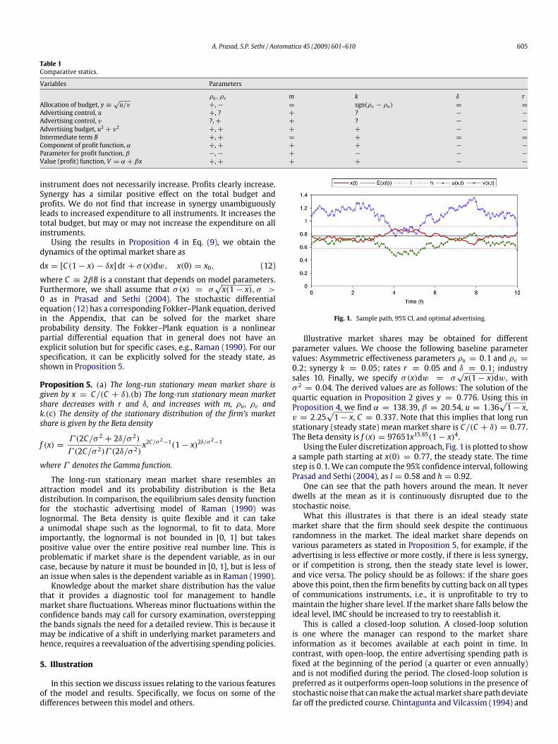
Fig. 1. Sample path, 95% CI, and optimal advertising.

Illustrative market shares may be obtained for differentparameter values. We choose the following baseline parametervalues: Asymmetric effectiveness parameters ρu = 0.1 and ρv =0.2; synergy k = 0.05; rates r = 0.05 and δ = 0.1; industrysales 10. Finally, we specify σ(x)dw = σ

√x(1− x)dw, with

σ 2 = 0.04. The derived values are as follows: The solution of thequartic equation in Proposition 2 gives y = 0.776. Using this inProposition 4, we find α = 138.39, β = 20.54, u = 1.36

√1− x,

v = 2.25√1− x, C = 0.337. Note that this implies that long run

stationary (steady state) mean market share is C/(C + δ) = 0.77.The Beta density is f (x) = 97651x15.85(1− x)4.Using the Euler discretization approach, Fig. 1 is plotted to show

a sample path starting at x(0) = 0.77, the steady state. The timestep is 0.1.We can compute the 95% confidence interval, followingPrasad and Sethi (2004), as l = 0.58 and h = 0.92.One can see that the path hovers around the mean. It never

dwells at the mean as it is continuously disrupted due to thestochastic noise.What this illustrates is that there is an ideal steady state

market share that the firm should seek despite the continuousrandomness in the market. The ideal market share depends onvarious parameters as stated in Proposition 5, for example, if theadvertising is less effective or more costly, if there is less synergy,or if competition is strong, then the steady state level is lower,and vice versa. The policy should be as follows: if the share goesabove this point, then the firm benefits by cutting back on all typesof communications instruments, i.e., it is unprofitable to try tomaintain the higher share level. If the market share falls below theideal level, IMC should be increased to try to reestablish it.This is called a closed-loop solution. A closed-loop solution

is one where the manager can respond to the market shareinformation as it becomes available at each point in time. Incontrast, with open-loop, the entire advertising spending path isfixed at the beginning of the period (a quarter or even annually)and is not modified during the period. The closed-loop solution ispreferred as it outperforms open-loop solutions in the presence ofstochastic noise that canmake the actualmarket share pathdeviatefar off the predicted course. Chintagunta and Vilcassim (1994) and

606 A. Prasad, S.P. Sethi / Automatica 45 (2009) 601–610

Erickson (1992) provide evidence that a closed-loop solution fitsempirical data better than its open-loop counterpart. Raman andNaik (2004) compute a closed-loop solution, but the nature ofthe dynamics there ensures that advertising is independent ofsales. Closed-loop solutions for IMC models where advertisingdepends on sale have not been previously computed due to theirdifficulty, and it is a useful feature of themodel and the underlyingframework, that all the analysis goes through.

6. Generalizations

In this section we shall extend the model to multipleinstruments and multiple competitors. First we show a generalresult. Consider the IMC model

Maxu1(t),u2(t),...,un(t)

J

=

∫∞

0e−rt (mx(t)− C(u1(t), u2(t), . . . , un(t))) dt,

s.t. dx(t) = G(U(u1(t), u2(t), . . . , un(t)), x(t), t)dt+ σ(x(t))dw(t).

(13)

Here G is increasing in U , and C and U in their arguments.Almost all existing IMC models fit in this framework as evidentfrom the literature review, the exception is Naik et al. (2005)wherethe promotion control affects the margin. For example, the formsC(u, v) = u2 + v2 (Chintagunta & Vilcassim, 1994; Fruchter &Kalish, 1998; Naik & Raman, 2003; Raman &Naik, 2004), C(u, v) =u+ v (Gopalakrishna & Chatterjee, 1992), U(u, v) = ρuu+ ρvv +kuv (all reviewed IMCmodels), or U(u, v) = ρuu+ρvv+ k

√uv as

in the proposed model, have all been used. We then observe thatthe following result will hold:

Proposition 6. The optimization problem (13) is equivalent to thefollowing two sub-problems:• The allocation problem

Maxu1(t),u2(t),...,un(t)

U(u1(t), u2(t), . . . , un(t)),

s.t. C(u1(t), u2(t), . . . , un(t)) = b(t)2.(14)

• The budgeting problem

Maxb(t)J =

∫∞

0e−rt

(mx(t)− b(t)2

)dt,

s.t. dx(t) = G(f (b(t)), x(t), t)dt + σ(x(t))dw(t).(15)

Here, we follow the convention of keeping the budget termb(t)2 in squared form. The sub-problems state; given a budgetwhat is its best allocation among the instruments, and given theoptimized allocation (IMC) what size of budget should be picked.Whereas the budgeting problem has been studied for a long time,it is the allocation problem that truly captures the unique goal ofIMC— coordinating the instruments to provide clarity, consistencyand maximum communications impact.It is useful to see that the allocation problem can be solved in a

staticmanner. There are great implementation benefits to realizingthat the allocation and budgeting problems can be independent.For example, in simulations of the type done by Gopalakrishnaand Chatterjee (1992), which could have been done with a singledynamic control instead of four, the simulation would be simplerand more accurate, particularly over a larger number of periods.

6.1. Multiple instruments

So far we have considered the situation where the firmadvertises in two media, which is the minimum number forinteraction effects to occur. The purpose of this section is to extendthe model and analysis to the case of three or more media. Given

the great range of media options — TV, radio, internet, billboardsetc., it is not uncommon that a firm would be advertising in morethan two. Hence,wewould like to extend the previously developedtheory to cover these cases. Since the expressions can becomequite lengthy, we shall focus primarily on the three-media case.However, from the symmetry of the equations, it will be clearthat the same technique can be used to study cases with a largernumber of media.Let u, v and w represent the three advertising decisions.

Analogous to the two media case, the objective function for thefirm is given by

Maxu,v,w≥0

{V (x0) = E

∫∞

0e−rt(mx− u2 − v2 − w2)dt

},

s.t. dx =[U(u, v, w)

√1− x− δx

]dt + σ(x)dw, x(0) = x0,

U(u, v, w) ≡ ρuu+ ρvv + ρww + ρuv√uv + ρuw

√uw

+ ρvw√vw + ρuvw(uvw)1/3,

r,m, δ, ρu, ρv, ρw, ρuv, ρuw, ρvw, ρuvw > 0, x0 ∈ [0, 1].

(16)

As before, the firm selects its advertising decisions to maximizeits expected, discounted profit stream subject to the market sharedynamics. But, here, there is more than one synergy parameter;in fact there are four ways in which the media can interact twoor three at a time. In contrast to previous literature, three-way orhigher interactions can be analyzed. With nmedia, the number ofinteraction terms will be 2n − n − 1. It should also be noted thatthe units are kept consistent, i.e., we have the term (uvw)1/3 in thethree-media case, whereas in the four-media case, there will be afourth root term.Consider the allocation problem first. Note that the fact that the

problem can be broken into two sub-problems does not guaranteethat it can be easily solved. While the allocation problem isstatic, there is no guarantee that the function f (b) will be simple.Preferablywewould like it to be linear so that the problem reducesto a single control problem that has been examined in the literatureand leads to a solvable dynamic optimization problem, e.g., to theSethi (1983) model, which among models of a single instrument,allows for inclusion of stochasticity, competition, closed loop andexplicit solutions.It should be remarked that the selectedU(u, v, w) specification

is the only one that has this property. This is because with thedesire that f (b) should be linear in b, we require each term in theoptimized U(u, v, w) to be linear in b. Thus if u = φ1b, v = φ2b,w = φ3b, then the remaining terms will be linear only with theuse of the square root (for 2 variable interactions) and cube root(for 3-variable interaction). Thus unnecessary nonlinearities arenot introduced into the analysis.Collecting the results of the analysis, we get Proposition 7which

bears a close correspondence with the analysis of the two-mediacase.

Proposition 7. The optimization problem has a unique, closed-loopsolution. In particular,(a) the optimal advertising controls are positive and given by,

u = βA1√1− x, v = βA2

√1− x, w = βA3

√1− x

(b) the value function is V (x) = α + βx and the total discountedprofit is V (x0) = α + βx0,(c) the long-run stationary mean market share is given by x =

C/(C + δ), where the parameters α, β , C , A1, A2 and A3 are given by

α =mr

(1−

2

1+√1+ 4Bm/(r + δ)2

)

β =2m

(r + δ)+√(r + δ)2 + 4Bm

A. Prasad, S.P. Sethi / Automatica 45 (2009) 601–610 607

and where, B ≡ A21 + A22 + A

23, and C ≡ 2βB, and A1, A2 and A3

simultaneously solve

ρuA1 + ρuv√A1A2/2+ ρuw

√A1A3/2+ ρuvw(A1A2A3)1/3/3 = 2A21,

ρvA2 + ρuv√A1A2/2+ ρvw

√A2A3/2+ ρuvw(A1A2A3)1/3/3 = 2A22,

ρwA3+ ρuw√A1A3/2+ ρvw

√A2A3/2+ ρuvw(A1A2A3)1/3/3 = 2A23.

Thus the dynamic optimization problem is reduced to thesimpler problem of finding the solutions of the three simultaneousequations (or n simultaneous equations in the n-media case.) Thiscan be done by numerical methods, such as the Gauss–Seidelalgorithm, which converges rapidly given that the objective isglobally concave. The form of the results is similar to the two-control case since the budgeting sub-problem in both cases isthe single variable Sethi (1983) model. Extending this to evenmore instruments is straightforward, so this is a flexible theory toanalyze multi-media problems involving synergy.

6.2. Competition

The advantage of separating the problem into a static allocationproblem and dynamic budgeting problem is that the dynamicproblem becomes a single control problem. And by using thespecification

U(u, v, w) ≡ ρuu+ ρvv + ρww + ρuv√uv + ρuw

√uw

+ ρvw√vw + ρuvw(uvw)1/3

the allocation sub-problem will provide a solution that leads to adynamic equation that can be linear in the control (e.g., if G is alsolinear in U and C is quadratic).As such, inclusion of competition is not complicated because

there already exist many stochastic differential games of a singlecontrol variable that can be readily applied. In particular, we canuse the duopoly model discussed in Chintagunta and Jain (1995),Prasad and Sethi (2004) and Sorger (1989):

Maxu1≥0

{V1(x0) = E

∫∞

0e−r1t [m1x(t)− b1(t)2]dt

},

Maxu2>0

{V2(x0) = E

∫∞

0e−r2t [m2(1− x(t))− b2(t)2]dt

},

s.t., dx = [ρ1b1(x)√1− x− ρ2b2(x)

√x]dt + σ(x)dw, x(0) = x0 ∈

[0, 1], where x is the market share of firm 1 and (1 − x) is themarket share of firm 2. Since the dynamic equation constraint forfirm 2 is totally captured by the dynamic equation for firm 1, thereis no need to write it as part of the problem. Here b1 and b2 are thesolutions from each firm’s allocation sub-problem as before. ThePrasad and Sethi (2004) paper also has a term that captures churneffects, which we need not discuss here, but it can be included ifneeded. The explicit solution is provided in that paper and hencewe omit it here to save space.To summarize, the paper developed a generalmodel of IMC that

combines several relevant factors, such as stochasticity, strategiccompetition andmultiple instruments, and is explicitly solvable forclosed loop strategies.

7. Conclusions

The concept of Integrated Marketing Communications (IMC)has become very important for advertisers and decision makersin the last decade. IMC seeks to leverage the synergy betweendifferent communications activities. There is no doubt that IMCis a well established theory. Empirical studies have shown thatsynergy between communicationsmix elements can be significant.A number of marketing mix models have operationalized synergyas an interaction term. Such models can be quite difficult to

solve analytically or even numerically, particularly when a closed-loop solution and/or presence of uncertainty are called for. Andincluding competition or more than 2 instruments is also adifficult task. Yet ignoring synergy when it exists is obviouslysuboptimal too.In this paper we are able to develop an IMC model where

explicit closed-loop solutions can be obtained for a firm withmultiple communications instruments, even in the presence ofuncertainty. Uncertainty in advertising is modeled through thewell-known stochastic differential equation approach. The paperextends the work of Fruchter and Kalish (1998) to include IMCand explicit solutions, and of Naik and Raman (2003) to multiplemedia, and of both to advertising interaction with sales, strategiccompetitors and stochastic analysis.Stochastic differential equations are hard to analyze, even

numerically. The reason is that for each guess of the optimaladvertising path, several sample market share paths must bedrawn in order to compute the expected profit. Analysis isfrequently done by excluding uncertainty in the theory butinserting it in the estimation stage. In contrast, the proposedmodel allows stochasticity to be handled analytically. The optimaladvertising decision depends only on the market share and noton the nature of the disturbance. In other words, the advertisingdecisions are robust to increase or decrease in uncertainty in themarket response to advertising. The intuition is that on average theincrease in profit from better response cancels out the decrease inprofits from poor responses.We find that positive expenditure on all communications

instruments is optimal if synergy exists, even if the instrumentis ineffectual in isolation (Proposition 1). In contrast to allocationin the absence of synergy, the ratio of advertising expendituresdoes not vary as the ratio of the square of the effectiveness ofthe advertising, but that the weaker instrument is allocated adisproportionately higher share of the budget (Proposition 2). Wefind that the allocation depends on factors such as the effectivenessof the different advertising, but that it is independent of factorssuch as discount rate or decay caused by forgetting, backgroundcompetition etc. (Proposition 3).We obtain a closed-loop solutionwhere the optimal advertising

depends on the current market share of the firm (Proposition 4).Results showed that the firm should do more advertising whenthe market share drops than when it is high, in contrast tothe affordability method or the percentage of sales methods ofadvertising budgeting (Proposition 4). The comparative statics inTable 1 summarize the effects of synergy. The total IMC budgetwould be lower and profitability would be lower if synergy werepresent in the marketplace but ignored in the firm’s analysis. Thefirm would be seeking a lower steady state market share. It isnot the case, however, that the expenditure on all instrumentswould drop. It might actually be higher in some, following fromthe discussion after Proposition 2, but there would be an incorrectallocation to the different media instruments.The steady state market share takes the form of an attraction

model, and its distribution, due to uncertainties in the market,follows a Beta distribution (Proposition 5). We show that thedecision on how much to allocate on different instruments ormedia is independent of the total IMC budget (Proposition 6). Weextend the model to multiple media and show that it can still besolved (Proposition 7). Finally, the model can include competitionwithout difficulty.Future research can extend the model to consider adding

penalty of modifying ad buys, or the premium for spot adbuying (Raman & Naik, 2004). Another generalization is to haveadvertising influence the noise term of the state equation inaddition to influencing the drift term as in the present case. Recentwork in this area has been done by Buratto and Grosset (2006)for a linear-quadratic, finite horizon model, with two advertisingcontrols where one control also affects the diffusion term.

608 A. Prasad, S.P. Sethi / Automatica 45 (2009) 601–610

The model can be empirically tested. Methods of estimatingstochastic differential equations (SDE) using discrete observationsare used in Finance for analyzing stocks, bonds and currenciestime series, and in Electrical engineering, for signal processing. Thesimplest method is Euler discretization followed by time-seriesestimation, the problembeing thatwithout adequate correction forunrecorded noise between the discrete time intervals, estimatescan be biased. If the SDE is linear (i.e., the drift componentis linear) one uses the Kalman Filter, as in Naik and Raman(2003). With nonlinear SDEs, as in our case, if the SDE can besolved,MaximumLikelihood estimation canbeused. Other optionsinclude the Extended Kalman Filter (e.g., Naik et al. (2008)),Method of SimulatedMoments,MCMCmethods, orNonparametricmethods.

Acknowledgements

The authors thank seminar participants at the University ofCalifornia Davis, Bond University, the University of Sydney, andthe 2005Marketing Science Conference in Atlanta for their helpfulcomments and suggestions.

Appendix A. Proof of propositions

Proof of Proposition 1. Weemploy the following standard proce-dure. In proving Proposition 1, we suppose that the value functionwe seek must satisfy Vx > 0. Later, in Proposition 3, we obtain thevalue function as the only solution of theHJB equationwith Vx > 0.The first-order conditions for a maximum are

−2u+ Vx

(ρu +

k√v

2√u

)√1− x = 0,

−2v + Vx

(ρv +

k√u

2√v

)√1− x = 0.

(A.1)

Note that the solutions are bounded away from zero, since theleft hand side of the first (respectively, second) equation goes to+∞ in the limit as u → 0 (respectively, v → 0), assuring aninterior solution. The second-order conditions for a maximum arealso satisfied.

Proof of Proposition 2. We express the first-order conditions interms of y. The conditions are

Vx

(ρu +

k2y

)√1− x = 2u and

Vx

(ρv +

ky2

)√1− x = 2v.

Dividing the two equations, since Vx > 0, and simplifying, we get

ky4 + 2ρvy3 − 2ρuy− k = 0. (A.2)

The solution depends only on the model parameters.The following calculations establish the second part of the

proposition. Starting with (A.2),

k(y4 − 1) = 2y(ρu − ρvy2)⇒ k(y− 1)(y+ 1)(y2 + 1) = 2y(

√ρu −√ρvy)(√ρu +√ρvy)

⇒ sgn(y− 1) = sgn(√ρu −√ρvy)

∴ y > 1⇒ ρu > ρv; y = 1⇒ ρu = ρv; y < 1⇒ ρu < ρv.

Finally, we show that there exists a unique, positive solution tothe quartic equation f (y) ≡ ky4 + 2ρvy3 − 2ρuy − k = 0. Bycontinuity, since f (0) is negative and f (∞) = +∞, there must

exist at least one root on the positive real number line. To showuniqueness, we show that f ′(y) > 0 at any solution point asfollows:

f ′(y)|f (y)=0 = 4ky3 + 6ρvy2 − 2ρu= 3ky3 + 4ρvy2 + (ky4 + 2ρvy3 − 2ρuy− k)+ k= 3ky3 + 4ρvy2 + k > 0. �

Proof of Proposition 3. From the proof of Proposition 2, we notethat f (y) ≡ ky4 + 2ρvy3 − 2ρuy − k = 0 and f ′(y) > 0 atthe solution point. Thus, for any parameter θ , from the implicitfunction theorem,

sgn(dydθ

)= −sgn

(∂ f∂θ

).

Hence, we get

dydρu

> 0,dydρv

< 0,dydm= 0,

dydδ= 0,

dydr= 0,

and

sgn(dy/dk) = −sgn(y4 − 1) = sgn(1− y) = sgn(ρv − ρu).

The last equality follows from Proposition 2. �

Appendix B

Proof of Proposition 4. We rewrite the first-order conditionsfrom Proposition 1 as

u2 =Vx2

(ρuu+

k√uv2

)√1− x,

v2 =Vx2

(ρvv +

k√uv2

)√1− x.

(B.1)

Hence,

2(u2 + v2) = Vx(ρuu+ ρvv + k√uv)√1− x (B.2)

and the HJB equation can be written as

rV = mx+ u2 + v2 − Vxδx+ σ(x)2Vxx/2. (B.3)

From the first-order conditions, using y ≡√u/v, we get

u = Vx

(2ρuy+ k4y

)√1− x,

v = Vx

(2ρv + ky4

)√1− x,

(B.4)

and insert them into the HJB equation to obtain the Hamil-ton–Jacobi equation

rV = mx+ V 2x

[(2ρuy+ k4y

)2+

(2ρv + ky4

)2](1− x)− Vxδx

+ σ(x)2Vxx/2. (B.5)

It can be seen that the linear value function

V = α + βx (B.6)

satisfies this equation. Inserting it into the Hamilton–Jacobiequation, we get

rα + rβx = mx+ β2B(1− x)− βδx, (B.7)

where we denoted the term in square brackets in (B.5) as B.Comparing coefficients of like powers, we get

α = β2B/r and (r + δ)β = m− β2B. (B.8)

A. Prasad, S.P. Sethi / Automatica 45 (2009) 601–610 609

Thus, we see α > 0. As for β , we take the positive root. Thus, thesolution is

β =−(r + δ)+

√(r + δ)2 + 4Bm2B

=2m

(r + δ)+√(r + δ)2 + 4Bm

(B.9)

α = (m− (r + δ)β)/r =mr

(1−

2

1+√1+ 4Bm/(r + δ)2

).

(B.10)

For the third part of the proposition, note that the comparativestatics for m, r and δ can be assessed simply by viewing theexpressions (B.4)–(B.10).For the remaining parameters (ρu, ρv and k), we sketch some

proofs below and the rest may be obtained from the authors toconserve space.We first examine the intermediate termB. Note that ∂α/∂B > 0,

∂β/∂B < 0, and ∂V/∂B > 0. Using f (y) = 0, we can rewrite B inthree ways, i.e.,

B =(2ρuy+ k4y

)2+

(2ρv + ky4

)2= (y4 + 1)

(ρv

2+ky4

)2=

(1y4+ 1

)(ρu

2+k4y

)2.

We will use whichever expression is most convenient forgetting unambiguous comparative statics. For example, themiddleexpression gives ∂B/∂ρu > 0. Similarly, ∂B/∂ρv > 0 and∂B/∂k > 0. Hence, we get all the remaining comparative statics,save those for the controls, which could not always be signed.However, note that the budget u2+v2 can bewritten asβ2B(1−

x) or as (β√B)2(1− x). The term

β√B = 2m

(r+δ)/√B+√(r+δ)2/B+4m

,and it is clear that it will have

the same comparative statics for ρu, ρv and k as B. �

Appendix C

Proof of Proposition 5. Using (B.2) and defining C = 2βB, we canwrite the optimal state dynamics

dx = [C(1− x)− δx] dt + σ(x)dw, x(0) = x0, (C.1)

as the stochastic integral equation

x(t) = x0 +∫ t

0(C − x(s) (C + δ)) ds+

∫ t

0σ(x)dw. (C.2)

The mean evolution path is independent of the nature of thestochastic disturbance. Specifically,

E[x(t)] = x0 +∫ t

0(C − E[x(s)] (C + δ)) ds. (C.3)

This can be expressed as an ordinary differential equation inE[x(t)], with the initial condition E[x(0)] = x0, whose solution isgiven by

E[x(t)] = exp[−(C + δ)t]x0 + (1− exp[−(C + δ)t])C/(C + δ).(C.4)

The long-run stationarymeanmarket share is limt→∞ E[x(t)] =C/(C + δ).This can bewritten as 1/(1+δ(r+δ+

√(r + δ)2 + 4Bm)/4mB).

By inspection, the long-run stationary mean market sharedecreases with r , δ, and increases with m and B. Also, recall that

∂B/∂ρu > 0, ∂B/∂ρv > 0 and ∂B/∂k > 0. It follows that the long-run stationary mean market share increases with ρu, ρv and k.For the final part, the solution x(t) of the Itô stochastic

differential equation

dx(t) = a(x, t)dt + b(x, t)dw(t), x(s) = z,

is aMarkov process, where the density of the transition probabilityp(t, x; s, z) for going frommarket share z at time s to market sharex at time t > s, satisfies the Fokker–Planck equation

∂p∂t+∂

∂x(ap)−

12∂2

∂x2(b2p) = 0,

p(t, x; t, z) = δ(x− z).

For the steady state density f (x) = limt→∞ p(t, x), we ignorethe initial transient part of the solution and set ∂p/∂t = 0.Writingthe Fokker–Planck equation for our case, we get the second-orderordinary differential equation

σ 2x(x− 1)2

d2fdx2+ ((2σ 2 − (C + δ))x+ C − σ 2)

dfdx

+ (σ 2 − (C + δ))f = 0.

This is identifiable as a Gaussian hypergeometric equationwith thesolution

f (x) = x2Cσ2−1(1− x)

2δσ2−1(C1 + C2

∫x−

2Cσ2 (1− x)

−2δσ2 dx

).

This corresponds to the Beta distribution

f (x) =Γ (2C/σ 2 + 2δ/σ 2)Γ (2C/σ 2)Γ (2δ/σ 2)

x2C/σ2−1(1− x)2δ/σ

2−1

where Γ denotes the Gamma function. Note that the densityintegrates to 1 by definition, while the mean of the distribution isgiven by C/(C + δ). �

Proof of Proposition 6. This follows the discussion in Sethi andZhang (1994, Section 5.4)).

Proof of Proposition 7. The HJB equation is given by

rV = Maxu,v,w>0

mx− u2 − v2 − w2 + Vx[(ρuu+ ρvv + ρww+ ρuv

√uv + ρuw

√uw + ρvw

√vw

+ ρuvw(uvw)1/3)√1− x− δx] + σ 2Vxx/2.

(D.1)

The first-order conditions are

−2u+ Vx

[ρu + ρuv

√v

2√u+ ρuw

√w

2√u

+ ρuvw(vw)1/3

3u2/3

]√1− x = 0,

−2v + Vx

[ρv + ρuv

√u

2√v+ ρvw

√w

2√v

+ ρuvw(uw)1/3

3v2/3

]√1− x = 0,

−2w + Vx

[ρw + ρuw

√u

2√w+ ρvw

√v

2√w

+ ρuvw(uv)1/3

3w2/3

]√1− x = 0.

(D.2)

We note that the objective function is globally concave in u, vandw.

610 A. Prasad, S.P. Sethi / Automatica 45 (2009) 601–610

The terms inside square brackets in the first-order conditionsare independent of Vx or x, and depend only on model parameterssince the equations are satisfied by

u = A1Vx√1− x, v = A2Vx

√1− x,

w = A3Vx√1− x.

(D.3)

The constants A1, A2 and A3 solve the three equations in theProposition. Multiplying the equations in (D.2) by u, v and w andadding them, we can rewrite the HJB equation as rV = mx+ u2 +v2 + w2 − Vxδx+ σ 2Vxx/2, or

rV = mx+ (1− x)V 2x (A21 + A

22 + A

23)− Vxδx+ σ

2Vxx/2. (D.4)

We use the linear value function V = α + βx. Comparingcoefficients of like terms, we find, as before,

α = β2B/r and (r + δ)β = m− β2B, (D.5)

where B ≡ A21 + A22 + A

23. The solution for β is

β =−(r + δ)+

√(r + δ)2 + 4Bm2B

=2m

(r + δ)+√(r + δ)2 + 4Bm

α = (m− (r + δ)β)/r =mr

(1−

2

1+√1+ 4Bm/(r + δ)2

).

We can write the state dynamics as (15), where C ≡ 2βB. Thesteady state market share is C/(C + δ), and we can follow theprevious analysis to obtain the Beta density function for it.

References

Aaker, A., & Carman, J. M. (1982). Are you overadvertising? Journal of AdvertisingResearch, 22(4), 57–70.

Assmus, G., Farley, J. U., & Lehmann, D. R. (1984). How advertising affects sales:Meta-analysis of econometric results. Journal of Marketing Research, 21(1),65–74.

Bass, F. M., Krishnamoorthy, A., Prasad, A., & Sethi, S. P. (2005). Generic and brandadvertising strategies in a dynamic duopoly.Marketing Science, 24(4), 556–568.

Buratto, A., & Grosset, L. (2006). A communication mix for an event planning:A linear quadratic approach. Central European Journal of Operations Research,14(3), 247–259.

Buratto, A., Grosset, L., & Viscolani, B. (2006). Advertising channel selection in asegmented market. Automatica, 42(8), 1343–1347.

Chintagunta, P. K., & Jain, D. C. (1995). Empirical analysis of a dynamic duopolymodel of competition. Journal of Economics and Management Strategy, 4(1),109–131.

Chintagunta, P. K., & Vilcassim, N. J. (1994). Marketing investment decisions ina dynamic duopoly: A model and empirical analysis. International Journal ofResearch in Marketing , 11(3), 287–306.

Doyle, P., & Saunders, J. (1990). Multiproduct advertising budgeting. MarketingScience, 9(2), 97–113.

Erickson, G. M. (1992). Empirical analysis of closed-loop duopoly advertisingstrategies.Management Science, 38(2), 1732–1749.

Erickson, G. M. (2003). Dynamic models of advertising competition. Norwell, MA:Kluwer Academic Publishers.

Feichtinger, G., Hartl, R. F., & Sethi, S. P. (1994). Dynamic optimal control models inadvertising: Recent developments.Management Science, 40(2), 195–226.

Feinberg, F. M. (1992). Pulsing policies for aggregate advertising models.MarketingScience, 11(3), 221–234.

Fruchter, G. E., & Kalish, S. (1998). Dynamic promotional budgeting and mediaallocation. European Journal of Operations Research, 111(1), 15–27.

Gatignon, H., & Hanssens, D. M. (1987). Modeling marketing interactions withapplications to salesforce effectiveness. Journal of Marketing Research, 24(3),247–257.

Gopalakrishna, S., & Chatterjee, R. (1992). A communications response model for amature industrial product: Applications and implications. Journal of MarketingResearch, 29(2), 189–200.

Jagpal, H. S. (1981). Measuring joint advertising effects in multiproduct firms.Journal of Advertising Research, 21(1), 65–69.

Jorgensen, S., & Zaccour, G. (2004). Differential games in marketing. Norwell, MA:Kluwer Academic Publishers.

Joseph, K., & Richardson, V. J. (2002). Free cash flow, agency costs and theaffordability method of advertising budgeting. Journal of Marketing , 66(1),94–107.

Little, J. D. C. (1979). Aggregate advertising models: The state of the art. OperationsResearch, 27(4), 629–667.

Mahajan, V., & Muller, E. (1986). Advertising pulsing policies for generatingawareness for new products.Marketing Science, 5(2), 86–106.

Naik, P. A., Prasad, A., & Sethi, S. P. (2008). Building brand awareness in dynamicoligopoly markets.Management Science, 54(1), 129–138.

Naik, P. A., & Raman, K. (2003). Understanding the impact of synergy onmultimediacommunications. Journal of Marketing Research, 40(4), 375–388.

Naik, P. A., Raman, K., & Winer, R. S. (2005). Planning marketing-mix strategies inthe presence of interactions.Marketing Science, 24(1), 25–34.

Nerlove, M., & Arrow, K. J. (1962). Optimal advertising policy under dynamicconditions. Economica, 29(114), 129–142.

Prasad, A., & Sethi, S. P. (2004). Competitive advertising under uncertainty: Astochastic differential game approach. Journal of Optimization Theory andApplications, 123(1), 163–185.

Raman, K. (1990). Stochastically optimal advertising policies under dynamicconditions: The ratio rule. Optimal Control Applications and Methods, 11(3),283–288.

Raman, K. (2006). Boundary value problems in stochastic optimal control ofadvertising. Automatica, 42(8), 1357–1362.

Raman, K., & Naik, P. A. (2004). Long-term profit impact of integrated marketingcommunications program. Review of Marketing Science, 2(1), Article 8.

Schultz, D. E. (1993). Integrated marketing communications: Maybe definition is inthe point of view.Marketing News, 27(2), 17.

Sasieni, M. W. (1971). Optimal advertising expenditure.Management Science, 18(4),P64–P72.

Sasieni, M. W. (1989). Optimal advertising strategies. Marketing Science, 8(4),358–370.

Sethi, S. P. (1973). Optimal control of the Vidale–Wolfe advertising model.Operations Research, 21(4), 998–1013.

Sethi, S. P. (1983). Deterministic and stochastic optimization of a dynamicadvertising model. Optimal Control Applications and Methods, 4(2), 179–184.

Sethi, S. P., & Thompson, G. L. (2000). Optimal control theory: Applications tomanagement science and economics (2nd ed.). Boston, MA: Kluwer.

Sethi, S. P., & Zhang, Q. (1994). Hierarchical decision making in stochasticmanufacturing systems. Boston, MA: Birkhäuser.

Sorger, G. (1989). Competitive dynamic advertising: A modification of the casegame. Journal of Economics Dynamics and Control, 13(1), 55–80.

Vakratsas, D., Feinberg, F. M., Bass, F. M., & Kalyanaram, G. (2004). The shapeof advertising response functions revisited: A model of dynamic probabilisticthresholds.Marketing Science, 23(1), 109–119.

Vidale, M. L., & Wolfe, H. B. (1957). An operations research study of sales responseto advertising. Operations Research, 5(3), 370–381.

Villas-Boas, M. J. (1993). Predicting advertising pulsing policies in an oligopoly: Amodel and empirical test.Marketing Science, 12, 88–102.

Ashutosh Prasad is Associate Professor of Marketing atUT Dallas. He holds a Ph.D. in Marketing and M.S. in Eco-nomics from UT Austin. His research interests are in pric-ing and advertising strategies, the economics of informa-tion, and software marketing. He also actively researchessalesforce management issues such as compensation de-sign, internalmarketing, training andmotivation.Hisworkhas appeared in journals such as Marketing Science, Man-agement Science, Journal of Business, IJRM and Experi-mental Economics. His dissertation won the the IJRM bestpaper award. He also received the UTD outstanding un-

dergraduate teacher award. He serves as a reviewer for all the leading marketingjournals.

Suresh P. Sethi is Charles &Nancy DavidsonDistinguishedProfessor of Operations Management and Director of theCenter for Intelligent Supply Networks at TheUniversity ofTexas atDallas. Hehaswritten 5books andpublishedmorethan 300 research papers in the fields of manufacturingand operations management, finance and economics,marketing, and optimization theory. He teaches a courseon optimal control theory/applications and organizes aseminar series on operations research topics. Recenthonors include: IITB Distinguished Alum (2008), POMSFellow (2005), INFORMS Fellow (2003), AAAS Fellow

(2003), IEEE Fellow (2001). Two conferences were organized and two books editedin his honor in 2005–6.