Embed Size (px)
Citation preview

This work is licensed under a Creative Commons Attribution 4.0 International License
Newcastle University ePrints - eprint.ncl.ac.uk
Gao ZC, Chin CS, Woo WL, Jia JB. Integrated Equivalent Circuit and Thermal
Model for Simulation of Temperature-Dependent LiFePO4 Battery in Actual
Embedded Application. Energies 2017, 10(1), 85-85.
Copyright:
This is an open access article distributed under the Creative Commons Attribution License which permits
unrestricted use, distribution, and reproduction in any medium, provided the original work is properly
cited. (CC BY 4.0).
DOI link to article:
http://dx.doi.org/10.3390/en10010085
Date deposited:
26/01/2017

energies
Article
Integrated Equivalent Circuit and Thermal Model forSimulation of Temperature-Dependent LiFePO4Battery in Actual Embedded Application
Zuchang Gao 1, Cheng Siong Chin 2,*, Wai Lok Woo 3 and Junbo Jia 1
1 School of Engineering, Temasek Polytechnic, 21 Tampines Avenue 1, Singapore 529757, Singapore;[email protected] (Z.G.); [email protected] (J.J.)
2 School of Marine Science and Technology, Newcastle University, Newcastle upon Tyne NE1 7RU, UK3 School of Electrical and Electronic Engineering, Newcastle University, Newcastle upon Tyne NE1 7RU, UK;
[email protected]* Correspondence: [email protected]; Tel.: +44-65-6908-6013
Academic Editor: William HolderbaumReceived: 11 October 2016; Accepted: 4 January 2017; Published: 11 January 2017
Abstract: A computational efficient battery pack model with thermal consideration is essential forsimulation prototyping before real-time embedded implementation. The proposed model provides acoupled equivalent circuit and convective thermal model to determine the state-of-charge (SOC) andtemperature of the LiFePO4 battery working in a real environment. A cell balancing strategy appliedto the proposed temperature-dependent battery model balanced the SOC of each cell to increase thelifespan of the battery. The simulation outputs are validated by a set of independent experimentaldata at a different temperature to ensure the model validity and reliability. The results show a rootmean square (RMS) error of 1.5609 × 10⁻⁵ for the terminal voltage and the comparison between thesimulation and experiment at various temperatures (from 5 ◦C to 45 ◦C) shows a maximum RMSerror of 7.2078 × 10⁻⁵.
Keywords: lithium-ion battery; battery management system; convective thermal model; cell model;state-of-charge
1. Introduction
In recent years, interest has increased for lithium-ion (Li-ion) batteries [1–3] in power generationand renewable energy applications such as solar energy systems, wave-operated electrical generationsystems, wind turbines, battery electric vehicles (BEVs), and portable power storage devices. Comparedwith other commonly used batteries like lead acid, nickel cadmium (NiCd) and nickel metal hydride(NiMH), LiFePO4 is popular due to its high capacity, low self-discharge current, wide temperatureoperation range, and long service life that make them better candidates for many applications.However, lithium-ion batteries are sensitive to overcharging or discharging that could deteriorate theperformance resulting in a shorter lifetime [4]. The accurate SOC estimation is, therefore, necessary fora properly functioning LiFePO4 battery power system.
Since there is no sensor available to measure SOC directly, it is estimated from physicalmeasurements (such as the current, voltage and temperature) via the battery management system(BMS). Currently, a large variety of methods for battery SOC estimation is proposed in the literature.First, the standard measurement-based estimation approaches, such as the coulomb counting methodor ampere-hour (Ah) methods, as well as the open-circuit voltage (OCV) and impedance measurementmethods [5–9] give a more intuitive and reliable estimation. Second, the machine learning-basedestimation method (also called black-box method), such as artificial neural network (ANN) and
Energies 2017, 10, 85; doi:10.3390/en10010085 www.mdpi.com/journal/energies
Energies 2017, 10, 85 2 of 22
fuzzy logic (FL) methods [10–17] require high computational effort for extensive training on a largedataset. Lastly, the state-space model-based estimation using Kalman filter (KF) [18–20] increasesthe computational load of the BMS. Hence, these methods have its advantages and disadvantages.They mostly focus on estimating the SOC of a single cell and terminal voltage estimation withoutconsidering the SOC and temperature differences between the cells in a battery [13]. Few works havebeen performed to explore the SOC predictions of the battery pack (or multiple cells) system withtemperature variations due to the ambient condition and cells. However, the temperature-dependentbattery model with the convective heat transfer between the cells are often too complicated to realizefor the actual application, and the simulation model is not available.
In this paper, the battery pack model is proposed to simulate the influence of temperature [14,15]between cells and the effect of ambient temperature acting on the cells that are necessary for developinga more reliable SOC estimation and cell balancing algorithm. A total of 12 LiFePO4 cells in a series areused for the modeling and parameter identification process. The parameters are estimated online by aseries of lookup tables to provide a good compromise between the high fidelity and computationaleffort for integrated BMS implementation, where the lookup table uses an array of data to map inputvalues to output values, approximating a mathematical function. If the lookup table encountersan input that does not match any of the table’s pre-defined input values, the block interpolatesor extrapolates the output values based on nearby table values. Since table lookups and simpleestimations can be faster than mathematical function evaluations, using the lookup table methodcan result in a faster computational time. The SOC estimation algorithm of the battery pack andcell balancing strategy are implemented and validated using the experimental data collected in alaboratory. The battery model under different temperatures is included to improve the battery model.The experiment results show the feasibility of the proposed model for simulation prototyping beforethe actual implementation.
In summary, the contributions of the paper include a 12-cell temperature-dependent batterymodel with the convective heat transfer between cells to estimate the SOC of each cell for automaticpassive cell balancing. This work also provides a battery simulation prototyping platform to allowdifferent algorithms and battery cells to be simulated and implemented quickly using the SimulinkCoder to generate and execute C code from Simulink with less programming needed. The experimentsverify the battery model in both near zero and room temperatures (from 5 ◦C to 45 ◦C) using the actualduty cycle.
The paper is organized as follows: Section 2 models the battery pack. It is followed by Section 3that deals with the experimental setup and data acquisition. The simulation model validation usingindependent experimental data, SOC estimation of the proposed battery pack and cell balancing arepresented in Section 4. Finally, Section 5 concludes the work with the future plan.
2. Battery Cell Model Description
The electrochemical model is the most accurate battery model for estimating the SOC. However,the electrochemical models are quite complex and involve partial differential equations [13] to solvein real-time. The black-box models using machine learning have recently been proposed. However,they use much computational effort for training large datasets for real-time embedded applicationsthat slow down the system’s output and performance in real-time. The alternative approach is to usethe equivalent circuit models (ECM) with a combination of voltage sources, resistors, and capacitorsto model the battery behaviors that will provide an interpretable structure for online estimationand implementation.
2.1. Equivalent Circuit Model
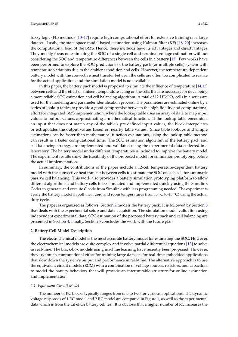
The number of RC blocks typically ranges from one to two for various applications. The dynamicvoltage responses of 1 RC model and 2 RC model are compared in Figure 1, as well as the experimentaldata which is from the LiFePO4 battery cell test. It is obvious that a higher number of RC increases the
Energies 2017, 10, 85 3 of 22
computational resources without significantly improving the model accuracy. Therefore, 1 RC batterycell model is proposed for the embedded applications in this paper, the model structure is shown inFigure 2.Energies 2017, 10, 85 3 of 22
Figure 1. Comparison of 1 RC and 2 RC fitting.
I
U1
UOC
R1
C1
R0
Rsd
Cb
UsocIUL
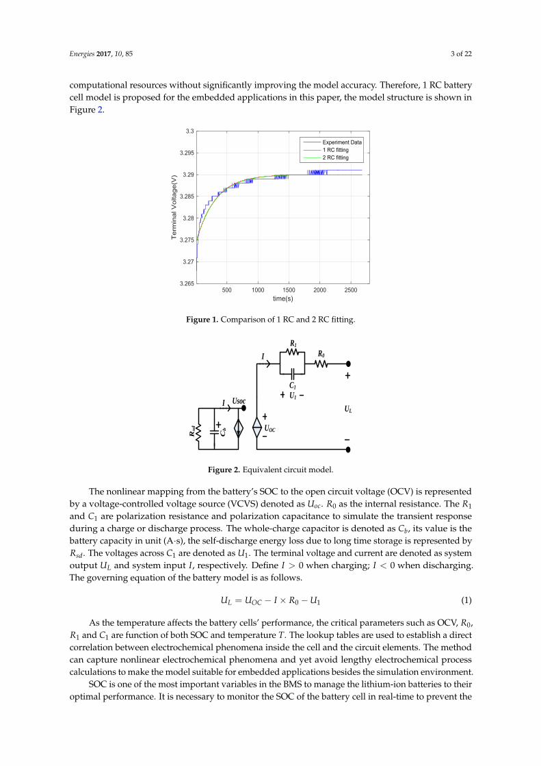
Figure 2. Equivalent circuit model
The nonlinear mapping from the battery’s SOC to the open circuit voltage (OCV) is represented
by a voltage-controlled voltage source (VCVS) denoted as 𝑈𝑜𝑐. 𝑅0 as the internal resistance. The 𝑅1
and 𝐶1 are polarization resistance and polarization capacitance to simulate the transient response
during a charge or discharge process. The whole-charge capacitor is denoted as 𝐶𝑏, its value is the
battery capacity in unit (A ∙ s), the self-discharge energy loss due to long time storage is represented
by 𝑅𝑠𝑑. The voltages across 𝐶1 are denoted as 𝑈1. The terminal voltage and current are denoted as
system output 𝑈𝐿 and system input 𝐼 , respectively. Define 𝐼 > 0 when charging; 𝐼 < 0 when
discharging. The governing equation of the battery model is as follows.
𝑈𝐿 = 𝑈𝑂𝐶 − 𝐼 × 𝑅0 − 𝑈1 (1)
As the temperature affects the battery cells’ performance, the critical parameters such as OCV,
𝑅0, 𝑅1 and 𝐶1 are function of both SOC and temperature 𝑇. The lookup tables are used to establish
a direct correlation between electrochemical phenomena inside the cell and the circuit elements. The
method can capture nonlinear electrochemical phenomena and yet avoid lengthy electrochemical
process calculations to make the model suitable for embedded applications besides the simulation
environment.
SOC is one of the most important variables in the BMS to manage the lithium-ion batteries to
their optimal performance. It is necessary to monitor the SOC of the battery cell in real-time to prevent
the battery cell from either undercharging or over-discharging as any of these conditions could
damage the battery cell permanently. In this paper, the Ah method is used to compute the SOC.
Figure 1. Comparison of 1 RC and 2 RC fitting.
Energies 2017, 10, 85 3 of 22
Figure 1. Comparison of 1 RC and 2 RC fitting.
I
U1
UOC
R1
C1
R0
Rsd
Cb
UsocIUL
Figure 2. Equivalent circuit model
The nonlinear mapping from the battery’s SOC to the open circuit voltage (OCV) is represented
by a voltage-controlled voltage source (VCVS) denoted as 𝑈𝑜𝑐. 𝑅0 as the internal resistance. The 𝑅1
and 𝐶1 are polarization resistance and polarization capacitance to simulate the transient response
during a charge or discharge process. The whole-charge capacitor is denoted as 𝐶𝑏, its value is the
battery capacity in unit (A ∙ s), the self-discharge energy loss due to long time storage is represented
by 𝑅𝑠𝑑. The voltages across 𝐶1 are denoted as 𝑈1. The terminal voltage and current are denoted as
system output 𝑈𝐿 and system input 𝐼 , respectively. Define 𝐼 > 0 when charging; 𝐼 < 0 when
discharging. The governing equation of the battery model is as follows.
𝑈𝐿 = 𝑈𝑂𝐶 − 𝐼 × 𝑅0 − 𝑈1 (1)
As the temperature affects the battery cells’ performance, the critical parameters such as OCV,
𝑅0, 𝑅1 and 𝐶1 are function of both SOC and temperature 𝑇. The lookup tables are used to establish
a direct correlation between electrochemical phenomena inside the cell and the circuit elements. The
method can capture nonlinear electrochemical phenomena and yet avoid lengthy electrochemical
process calculations to make the model suitable for embedded applications besides the simulation
environment.
SOC is one of the most important variables in the BMS to manage the lithium-ion batteries to
their optimal performance. It is necessary to monitor the SOC of the battery cell in real-time to prevent
the battery cell from either undercharging or over-discharging as any of these conditions could
damage the battery cell permanently. In this paper, the Ah method is used to compute the SOC.
Figure 2. Equivalent circuit model.
The nonlinear mapping from the battery’s SOC to the open circuit voltage (OCV) is representedby a voltage-controlled voltage source (VCVS) denoted as Uoc. R0 as the internal resistance. The R1
and C1 are polarization resistance and polarization capacitance to simulate the transient responseduring a charge or discharge process. The whole-charge capacitor is denoted as Cb, its value is thebattery capacity in unit (A·s), the self-discharge energy loss due to long time storage is represented byRsd. The voltages across C1 are denoted as U1. The terminal voltage and current are denoted as systemoutput UL and system input I, respectively. Define I > 0 when charging; I < 0 when discharging.The governing equation of the battery model is as follows.
UL = UOC − I × R0 − U1 (1)
As the temperature affects the battery cells’ performance, the critical parameters such as OCV, R0,R1 and C1 are function of both SOC and temperature T. The lookup tables are used to establish a directcorrelation between electrochemical phenomena inside the cell and the circuit elements. The methodcan capture nonlinear electrochemical phenomena and yet avoid lengthy electrochemical processcalculations to make the model suitable for embedded applications besides the simulation environment.
SOC is one of the most important variables in the BMS to manage the lithium-ion batteries to theiroptimal performance. It is necessary to monitor the SOC of the battery cell in real-time to prevent the

Energies 2017, 10, 85 4 of 22
battery cell from either undercharging or over-discharging as any of these conditions could damagethe battery cell permanently. In this paper, the Ah method is used to compute the SOC.
SOC(k) = SOC(0)− TCn
∫ k
0(η.i(t)− Sd)dt (2)
where SOC(0) is the initial SOC, Cn is the nominal capacity of the battery pack, T is the samplingperiod, i(t) is the load current at time t, η is coulombic efficiency, and Sd is the self-discharging rate.For LiFePO4 battery used in this experiment, η > 0.994 under room temperature [1]. In this paper,η = 1, and Sd = 0 are assumed.
The series connected cells’ capacity is the quantity of electric charge stored in the cells.Theoretically, the series battery capacity is given by the sum of the minimum capacity that canbe charged and discharged [2]:
Cseries = min1≤i≤m
(SOCi·Ci) + min1≤i≤m
((SOCi − 1)·Ci) (3)
where Cseries is the usable capacity of the series battery pack, Ci is the capacity of the i cell, SOCi isstate of charge of the i cell, m is the number of cells connected in a series.
2.2. Lumped-Capacitance Thermal Model of the Battery Cell
In this paper, the commercial LiFePO4 26650 cylindrical cells are selected to be the research objects,which are constructed in a multilayer structure in which the radial thermal conductivity is lower thanthe axial one. Nevertheless, the thermal resistance by the radial conduction is still much less than theconvective thermal resistance, as air is used as the coolant (i.e., the Biot number, Bi = Lch f /ks < 0.1).Therefore, a lumped-capacitance thermal model for battery cells assuming a uniform temperature ineach cell is sufficient without compromising accuracy of the numerical analysis. The thermal energybalance of the battery cell is modeled by using the first law of thermodynamics:
dUdt
= Qgen(t)− Qloss(t) (4)
where U represents the internal energy and is the total energy contained by a thermodynamic system(in joules). Qgen(t) is the generating heating rate, i.e., the rate of the heat generation occurring in the cell.
On the other hand, U can be determined by the following.
dU = m × CP × dTcell (5)
where m is the mass of the cell (in kilograms), dTcell is the temperature variation of the cell with time(in kelvin), and CP is the specific heat capacity of the cell (in J/kg/K).
The volume heat generation rate in a battery body is the sum of numerous local losses such asactive heat generation, reaction heat generation, and Ohmic heat generation. In this paper, Qgen(t)is characterized only by ohmic losses because of their simplicity to the model in the embeddedapplications. Ohmic losses are expressed as follows.
Qgen(t) = R0 × (I)2 + R1 × (I1)2 (6)
where I is the battery current, I1 is the current going through by R1.Moreover, Qloss(t) is a value of all the heat transfers as a result of a temperature difference between
the cells and the connections of the cells and consists of two parts: convective heat transfer Qconv andconductive heat transfer Qcond.
Qloss = Qconv + Qcond (7)
Energies 2017, 10, 85 5 of 22
1. Convective heat transfer
The convective heat transfer Qconv from the cell to the surrounding is determined by
Qconv = hconvSarea(Tcell − Tair) (8)
where hconv is the convective heat transfer coefficient, Sarea is the area of heat exchange, Tcell isthe cell temperature and Tair is the ambient temperature.
2. Conductive heat transfer
The convective heat transfer Qcond represents the thermal diffusion through cell to cell electricconnector. It can be modeled by
Qcond =Tcell2 − Tcell1
Rcond(9)
where Tcell2 and Tcell1 are the temperature of battery cell 2 and battery cell 1, respectively. Rcond isthe thermal resistance of the connection, which includes the top and bottom connection of thebattery cell.
In Li-ion battery, the cross-plane thermal conductivity is much smaller than the in-plane thermalconductivity. Heat conduction through the top and bottom of cells are important to the practicalsystem. However, in this study, the experimental battery cells are all brand new, assuming that theyare all with good uniformity. The temperature difference ∆T = Tcell2 − Tcell1 is ignored. As a result, theconductive heat transfer is also neglected in the model in the paper.
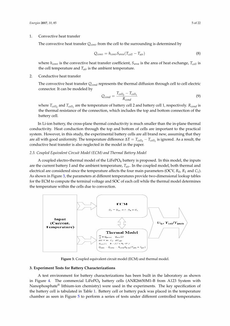
2.3. Coupled Equivalent Circuit Model (ECM) and Thermal Battery Model
A coupled electro-thermal model of the LiFePO4 battery is proposed. In this model, the inputsare the current battery I and the ambient temperature, Tair. In the coupled model, both thermal andelectrical are considered since the temperature affects the four main parameters (OCV, R0, R1 and C1).As shown in Figure 3, the parameters at different temperatures provide two-dimensional lookup tablesfor the ECM to compute the terminal voltage and SOC of each cell while the thermal model determinesthe temperature within the cells due to convection.
Energies 2017, 10, 85 5 of 22
2. Conductive heat transfer
The convective heat transfer represents the thermal diffusion through cell to cell electric connector. It can be modeled by = −
(9)
where and are the temperature of battery cell 2 and battery cell 1, respectively. is the thermal resistance of the connection, which includes the top and bottom connection
of the battery cell.
In Li-ion battery, the cross-plane thermal conductivity is much smaller than the in-plane thermal conductivity. Heat conduction through the top and bottom of cells are important to the practical system. However, in this study, the experimental battery cells are all brand new, assuming that they are all with good uniformity. The temperature difference ∆T = − is ignored. As a result, the conductive heat transfer is also neglected in the model in the paper.
2.3. Coupled Equivalent Circuit Model (ECM) and Thermal Battery Model
A coupled electro-thermal model of the LiFePO4 battery is proposed. In this model, the inputs are the current battery I and the ambient temperature, . In the coupled model, both thermal and electrical are considered since the temperature affects the four main parameters (OCV, , and ). As shown in Figure 3, the parameters at different temperatures provide two-dimensional lookup tables for the ECM to compute the terminal voltage and SOC of each cell while the thermal model determines the temperature within the cells due to convection.
Figure 3. Coupled equivalent circuit model (ECM) and thermal model
3. Experiment Tests for Battery Characterizations
A test environment for battery characterizations has been built in the laboratory as shown in Figure 4. The commercial LiFePO4 battery cells (ANR26650M1-B from A123 System with Nanophosphate® lithium-ion chemistry) were used in the experiments. The key specification of the battery cell is tabulated in Table 1. Battery cell or battery pack was placed in the temperature chamber as seen in Figure 5 to perform a series of tests under different controlled temperatures. The ambient temperatures 5 °C, 15 °C, 25 °C, 35 °C and 45 °C were used to determine the model parameters of the 12-cell battery. The load current is created using a programmable DC electronic load, and a programmable DC power supply for charging the battery cells. The power supply is utilized as a controlled voltage or current source with the output voltage from 0 to 36 V and current from 0 to 20 A. A current sensor LEM 50-P is used to measure the charge and discharge current. The NTC temperature sensors are utilized to measure the temperatures of the battery cells and the ambient temperature. The National Instruments DAQ device controlled all input and output data. The host
Figure 3. Coupled equivalent circuit model (ECM) and thermal model.
3. Experiment Tests for Battery Characterizations
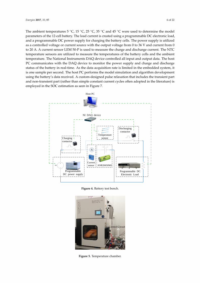
A test environment for battery characterizations has been built in the laboratory as shownin Figure 4. The commercial LiFePO4 battery cells (ANR26650M1-B from A123 System withNanophosphate® lithium-ion chemistry) were used in the experiments. The key specification ofthe battery cell is tabulated in Table 1. Battery cell or battery pack was placed in the temperaturechamber as seen in Figure 5 to perform a series of tests under different controlled temperatures.
Energies 2017, 10, 85 6 of 22
The ambient temperatures 5 ◦C, 15 ◦C, 25 ◦C, 35 ◦C and 45 ◦C were used to determine the modelparameters of the 12-cell battery. The load current is created using a programmable DC electronic load,and a programmable DC power supply for charging the battery cells. The power supply is utilizedas a controlled voltage or current source with the output voltage from 0 to 36 V and current from 0to 20 A. A current sensor LEM 50-P is used to measure the charge and discharge current. The NTCtemperature sensors are utilized to measure the temperatures of the battery cells and the ambienttemperature. The National Instruments DAQ device controlled all input and output data. The hostPC communicates with the DAQ device to monitor the power supply and charge and dischargestatus of the battery in real-time. As the data acquisition rate is limited in the embedded system, itis one sample per second. The host PC performs the model simulation and algorithm developmentusing the battery’s data received. A custom-designed pulse relaxation that includes the transient partand non-transient part (rather than simple constant current cycles often adopted in the literature) isemployed in the SOC estimation as seen in Figure 7.
Energies 2017, 10, 85 6 of 22
PC communicates with the DAQ device to monitor the power supply and charge and discharge status
of the battery in real-time. As the data acquisition rate is limited in the embedded system, it is one
sample per second. The host PC performs the model simulation and algorithm development using
the battery’s data received. A custom-designed pulse relaxation that includes the transient part and
non-transient part (rather than simple constant current cycles often adopted in the literature) is
employed in the SOC estimation as seen in Figure 7.
DC
Programmable
DC power supply
Charging
contactor
Discharging
contactor
ANR26650M1
Programmable DC
Electronic Load
A
Current
sensor
Temperature
sensor
NI DAQ device
Host PC
Figure 4. Battery test bench.
Figure 5. Temperature chamber.
Control Circuit
Figure 4. Battery test bench.
Energies 2017, 10, 85 6 of 22
PC communicates with the DAQ device to monitor the power supply and charge and discharge status
of the battery in real-time. As the data acquisition rate is limited in the embedded system, it is one
sample per second. The host PC performs the model simulation and algorithm development using
the battery’s data received. A custom-designed pulse relaxation that includes the transient part and
non-transient part (rather than simple constant current cycles often adopted in the literature) is
employed in the SOC estimation as seen in Figure 7.
DC
Programmable
DC power supply
Charging
contactor
Discharging
contactor
ANR26650M1
Programmable DC
Electronic Load
A
Current
sensor
Temperature
sensor
NI DAQ device
Host PC
Figure 4. Battery test bench.
Figure 5. Temperature chamber.
Control Circuit
Figure 5. Temperature chamber.
Energies 2017, 10, 85 7 of 22
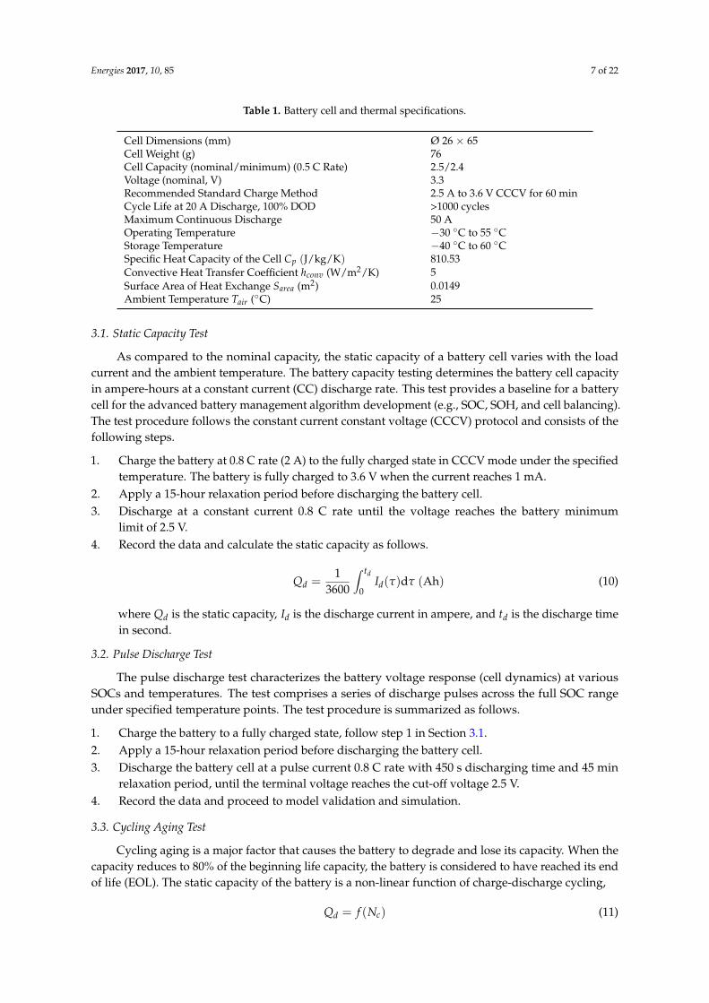
Table 1. Battery cell and thermal specifications.
Cell Dimensions (mm) Ø 26 × 65Cell Weight (g) 76Cell Capacity (nominal/minimum) (0.5 C Rate) 2.5/2.4Voltage (nominal, V) 3.3Recommended Standard Charge Method 2.5 A to 3.6 V CCCV for 60 minCycle Life at 20 A Discharge, 100% DOD >1000 cyclesMaximum Continuous Discharge 50 AOperating Temperature −30 ◦C to 55 ◦CStorage Temperature −40 ◦C to 60 ◦CSpecific Heat Capacity of the Cell Cp (J/kg/K) 810.53Convective Heat Transfer Coefficient hconv (W/m2/K) 5Surface Area of Heat Exchange Sarea (m2) 0.0149Ambient Temperature Tair (◦C) 25
3.1. Static Capacity Test
As compared to the nominal capacity, the static capacity of a battery cell varies with the loadcurrent and the ambient temperature. The battery capacity testing determines the battery cell capacityin ampere-hours at a constant current (CC) discharge rate. This test provides a baseline for a batterycell for the advanced battery management algorithm development (e.g., SOC, SOH, and cell balancing).The test procedure follows the constant current constant voltage (CCCV) protocol and consists of thefollowing steps.
1. Charge the battery at 0.8 C rate (2 A) to the fully charged state in CCCV mode under the specifiedtemperature. The battery is fully charged to 3.6 V when the current reaches 1 mA.
2. Apply a 15-hour relaxation period before discharging the battery cell.3. Discharge at a constant current 0.8 C rate until the voltage reaches the battery minimum
limit of 2.5 V.4. Record the data and calculate the static capacity as follows.
Qd =1
3600
∫ td
0Id(τ)dτ (Ah) (10)
where Qd is the static capacity, Id is the discharge current in ampere, and td is the discharge timein second.
3.2. Pulse Discharge Test
The pulse discharge test characterizes the battery voltage response (cell dynamics) at variousSOCs and temperatures. The test comprises a series of discharge pulses across the full SOC rangeunder specified temperature points. The test procedure is summarized as follows.
1. Charge the battery to a fully charged state, follow step 1 in Section 3.1.2. Apply a 15-hour relaxation period before discharging the battery cell.3. Discharge the battery cell at a pulse current 0.8 C rate with 450 s discharging time and 45 min
relaxation period, until the terminal voltage reaches the cut-off voltage 2.5 V.4. Record the data and proceed to model validation and simulation.
3.3. Cycling Aging Test
Cycling aging is a major factor that causes the battery to degrade and lose its capacity. When thecapacity reduces to 80% of the beginning life capacity, the battery is considered to have reached its endof life (EOL). The static capacity of the battery is a non-linear function of charge-discharge cycling,
Qd = f (Nc) (11)
Energies 2017, 10, 85 8 of 22
where Nc is the charge-discharge cycling number.The procedure of the one cycling test is illustrated as follows. The initial state of the battery is
assumed to be fully discharged.
1. Charge the battery to a fully charged state, follow step 1 in Section 3.1.2. Allow the battery to rest for 15 min until its temperature stabilized.3. Discharge at a constant current 0.8 C rate until the voltage reaches the battery minimum
limit of 2.5 V.4. Record the data and proceed to another cycle after the battery rests for 15 min.
Based on the cycling aging testing designed above and the manufacturer’s specifications in Table 1,the test will take around one year to perform. Thus, it is quite time-consuming to conduct such test.Since new battery cells were used in the experiment, the aging effect of the cells is therefore neglected.
4. Battery Model Identification and Results
4.1. Temperature-Dependent Battery Cell Parameters Identification
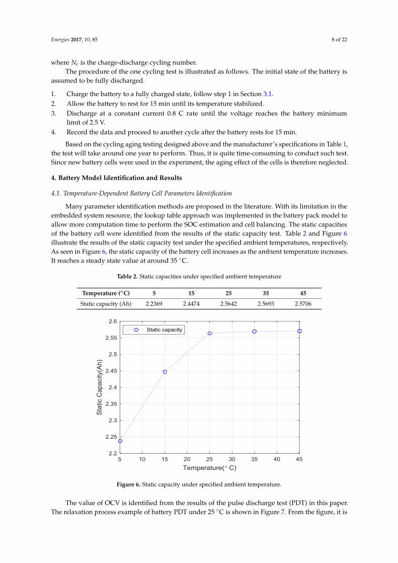
Many parameter identification methods are proposed in the literature. With its limitation in theembedded system resource, the lookup table approach was implemented in the battery pack model toallow more computation time to perform the SOC estimation and cell balancing. The static capacitiesof the battery cell were identified from the results of the static capacity test. Table 2 and Figure 6illustrate the results of the static capacity test under the specified ambient temperatures, respectively.As seen in Figure 6, the static capacity of the battery cell increases as the ambient temperature increases.It reaches a steady state value at around 35 ◦C.
Table 2. Static capacities under specified ambient temperature
Temperature (◦C) 5 15 25 35 45
Static capacity (Ah) 2.2369 2.4474 2.5642 2.5693 2.5706
Energies 2017, 10, 85 8 of 22
where 𝑁𝑐 is the charge-discharge cycling number.
The procedure of the one cycling test is illustrated as follows. The initial state of the battery is
assumed to be fully discharged.
1. Charge the battery to a fully charged state, follow step 1 in Section 3.1.
2. Allow the battery to rest for 15 min until its temperature stabilized.
3. Discharge at a constant current 0.8 C rate until the voltage reaches the battery minimum limit of
2.5 V.
4. Record the data and proceed to another cycle after the battery rests for 15 min.
Based on the cycling aging testing designed above and the manufacturer’s specifications in Table
1, the test will take around one year to perform. Thus, it is quite time-consuming to conduct such test.
Since new battery cells were used in the experiment, the aging effect of the cells is therefore neglected.
4. Battery Model Identification and Results
4.1. Temperature-Dependent Battery Cell Parameters Identification
Many parameter identification methods are proposed in the literature. With its limitation in the
embedded system resource, the lookup table approach was implemented in the battery pack model
to allow more computation time to perform the SOC estimation and cell balancing. The static
capacities of the battery cell were identified from the results of the static capacity test. Table 2 and
Figure 6 illustrate the results of the static capacity test under the specified ambient temperatures,
respectively. As seen in Figure 6, the static capacity of the battery cell increases as the ambient
temperature increases. It reaches a steady state value at around 35 °C.
Table 2. Static capacities under specified ambient temperature
Temperature (°C) 5 15 25 35 45
Static capacity (Ah) 2.2369 2.4474 2.5642 2.5693 2.5706
Figure 6. Static capacity under specified ambient temperature
Figure 6. Static capacity under specified ambient temperature.
The value of OCV is identified from the results of the pulse discharge test (PDT) in this paper.The relaxation process example of battery PDT under 25 ◦C is shown in Figure 7. From the figure, it is

Energies 2017, 10, 85 9 of 22
obvious that the difference of the terminal voltage between 45 min and 3 h is 0.02 mV (0.06% of thenominal voltage). Hence, to save the experiment time, 45 min was thought to be enough for relaxationdue to the small change in the terminal voltage after 45 min for the selected LiFeO4 battery.
Compared with low-rate current charge/discharge method, the proposed PDT method to obtainthe OCV at certain SOC intervals (e.g., 10%) can reduce the measurement time by around 90%.The comparison of C/50 low-rate discharge profile and the 10% SOC step incremental OCV curveat 25 ◦C is shown in Figure 8.
Energies 2017, 10, 85 9 of 22
The value of OCV is identified from the results of the pulse discharge test (PDT) in this paper.
The relaxation process example of battery PDT under 25 °C is shown in Figure 7. From the figure, it
is obvious that the difference of the terminal voltage between 45 min and 3 h is 0.02 mV (0.06% of the
nominal voltage). Hence, to save the experiment time, 45 min was thought to be enough for relaxation
due to the small change in the terminal voltage after 45 min for the selected LiFeO4 battery.
Compared with low-rate current charge/discharge method, the proposed PDT method to obtain
the OCV at certain SOC intervals (e.g., 10%) can reduce the measurement time by around 90%. The
comparison of C/50 low-rate discharge profile and the 10% SOC step incremental OCV curve at 25 °C
is shown in Figure 8.
Figure 7. Relaxation process example of battery pulse discharge test (PDT).
Figure 8. Comparison of C/50 low-rate discharge profile and the 10% state-of-charge (SOC) step
incremental open-circuit voltage (OCV) curve (25 °C)
Figure 9 shows a full voltage curve sample of PDT with 45 min relaxation at 25 °C. OCV
approximates the terminal voltage of the battery at equilibrium state of every relaxation period. The
Figure 7. Relaxation process example of battery pulse discharge test (PDT).
Energies 2017, 10, 85 9 of 22
The value of OCV is identified from the results of the pulse discharge test (PDT) in this paper.
The relaxation process example of battery PDT under 25 °C is shown in Figure 7. From the figure, it
is obvious that the difference of the terminal voltage between 45 min and 3 h is 0.02 mV (0.06% of the
nominal voltage). Hence, to save the experiment time, 45 min was thought to be enough for relaxation
due to the small change in the terminal voltage after 45 min for the selected LiFeO4 battery.
Compared with low-rate current charge/discharge method, the proposed PDT method to obtain
the OCV at certain SOC intervals (e.g., 10%) can reduce the measurement time by around 90%. The
comparison of C/50 low-rate discharge profile and the 10% SOC step incremental OCV curve at 25 °C
is shown in Figure 8.
Figure 7. Relaxation process example of battery pulse discharge test (PDT).
Figure 8. Comparison of C/50 low-rate discharge profile and the 10% state-of-charge (SOC) step
incremental open-circuit voltage (OCV) curve (25 °C)
Figure 9 shows a full voltage curve sample of PDT with 45 min relaxation at 25 °C. OCV
approximates the terminal voltage of the battery at equilibrium state of every relaxation period. The
Figure 8. Comparison of C/50 low-rate discharge profile and the 10% state-of-charge (SOC) stepincremental open-circuit voltage (OCV) curve (25 ◦C).
Figure 9 shows a full voltage curve sample of PDT with 45 min relaxation at 25 ◦C. OCVapproximates the terminal voltage of the battery at equilibrium state of every relaxation period.The OCV-SOC relationship curves under different temperatures are shown in Figure 10. As observedin Figure 10a, there is a higher OCV for the SOC value from 0.1 to 0.9. Also reflected in the close

Energies 2017, 10, 85 10 of 22
view as shown in Figure 10b, is a different OCV between various temperatures. When SOC is 0.2, themaximum OCV is approximately 25 mV with SOC error of 10% which is between 5 ◦C and 45 ◦C.Therefore, the OCV cannot be represented by simply a curve fitting method (that is commonly adoptedin the literature) to improve the accuracy of the OCV-SOC curve. From the Figure 8, 11 OCV datapoints can be gained for a full discharge period, which is 0~1 with the 10% SOC intervals. However,they might be insufficient to reflect all electrode features due to the low resolution. Interpolation is acommon method to yield additional data. Here, we applied interpolation method for better resolutionand as a result of reducing measurement time. Therefore, a lookup table with interpolation techniquesis applied to obtain the real-time OCV under different temperatures. The lookup table is created andstored in the embedded microcontroller. The curves of the OCV are illustrated in Figure 11. Withvarious SOCs and temperatures, the corresponding OCV can be obtained from the lookup table.
Energies 2017, 10, 85 10 of 22
OCV-SOC relationship curves under different temperatures are shown in Figure 10. As observed in
Figure 10a, there is a higher OCV for the SOC value from 0.1 to 0.9. Also reflected in the close view
as shown in Figure 10b, is a different OCV between various temperatures. When SOC is 0.2, the
maximum OCV is approximately 25 mV with SOC error of 10% which is between 5 °C and 45 °C.
Therefore, the OCV cannot be represented by simply a curve fitting method (that is commonly
adopted in the literature) to improve the accuracy of the OCV-SOC curve. From the Figure 8, 11 OCV
data points can be gained for a full discharge period, which is 0~1 with the 10% SOC intervals.
However, they might be insufficient to reflect all electrode features due to the low resolution.
Interpolation is a common method to yield additional data. Here, we applied interpolation method
for better resolution and as a result of reducing measurement time. Therefore, a lookup table with
interpolation techniques is applied to obtain the real-time OCV under different temperatures. The
lookup table is created and stored in the embedded microcontroller. The curves of the OCV are
illustrated in Figure 11. With various SOCs and temperatures, the corresponding OCV can be
obtained from the lookup table.
Figure 9. Terminal voltage of pulse discharges test.
Figure 10. (a) OCV-SOC relationship curves under different temperatures; (b) detailed view from
SOC 0.1 to 0.4.
Figure 9. Terminal voltage of pulse discharges test.
Energies 2017, 10, 85 10 of 22
OCV-SOC relationship curves under different temperatures are shown in Figure 10. As observed in
Figure 10a, there is a higher OCV for the SOC value from 0.1 to 0.9. Also reflected in the close view
as shown in Figure 10b, is a different OCV between various temperatures. When SOC is 0.2, the
maximum OCV is approximately 25 mV with SOC error of 10% which is between 5 °C and 45 °C.
Therefore, the OCV cannot be represented by simply a curve fitting method (that is commonly
adopted in the literature) to improve the accuracy of the OCV-SOC curve. From the Figure 8, 11 OCV
data points can be gained for a full discharge period, which is 0~1 with the 10% SOC intervals.
However, they might be insufficient to reflect all electrode features due to the low resolution.
Interpolation is a common method to yield additional data. Here, we applied interpolation method
for better resolution and as a result of reducing measurement time. Therefore, a lookup table with
interpolation techniques is applied to obtain the real-time OCV under different temperatures. The
lookup table is created and stored in the embedded microcontroller. The curves of the OCV are
illustrated in Figure 11. With various SOCs and temperatures, the corresponding OCV can be
obtained from the lookup table.
Figure 9. Terminal voltage of pulse discharges test.
Figure 10. (a) OCV-SOC relationship curves under different temperatures; (b) detailed view from
SOC 0.1 to 0.4. Figure 10. (a) OCV-SOC relationship curves under different temperatures; (b) detailed view fromSOC 0.1 to 0.4.

Energies 2017, 10, 85 11 of 22Energies 2017, 10, 85 11 of 22
Figure 11. OCV-SOC value curves.
In this Section, 𝑅1, 𝐶1 and 𝑅0 are identified from the results of PDT. Figure 12 is the relaxation
cycle used to identify these parameters. The DC internal resistance 𝑅0 is calculated from the
instantaneous rise of voltage using the following equation.
𝑅0,𝑛 =𝑈𝑛 − 𝑈𝑛−1
𝐼 (12)
where 𝑈𝑛 is the terminal voltage of sample 𝑛, and 𝐼 is the discharge current.
The abovementioned 𝑅0 is identified using the segment marked in red color shown in Figure
12. 𝑅1 and 𝐶1 represent the transient response of the battery voltage during the relaxation period.
The identification process starts in the segment marked in green color as shown in Figure 12. The
values of each parameter of the RC networks can be identified. The identified values will be tabulated
in the 2-D lookup tables as shown in Figures 13–15. The experiments were conducted at the following
temperatures 5 °C, 15 °C, 25 °C and 45 °C in order to include the influence of the ambient temperature
to parameters 𝑅0, 𝑅1 and 𝐶1. In this paper, a simplified lookup table with interpolation technique
is applied to obtain the real-time OCV, 𝑅1 and 𝐶1 , which is a highly efficient method for the
microcontroller in the embedded applications. Compared with other models with a complex
identified process such as adaptive least square (ALS) and extended Kalman filter (EKF), this method
reduces the burden on the processor greatly without large deficiency in performance. Table 3 shows
the comparison result of 𝑅0 identification, which obtains the 𝑅0 value by the ALS method, EKF
method and lookup table method implemented in the MATLAB environment, respectively. As
shown in Table 3, the lookup table method can save much identification time without big differences
in RMS.
Figure 12. Relaxation period after the discharge pulses.
Figure 11. OCV-SOC value curves.
In this Section, R1, C1 and R0 are identified from the results of PDT. Figure 12 is the relaxation cycleused to identify these parameters. The DC internal resistance R0 is calculated from the instantaneousrise of voltage using the following equation.
R0,n =Un − Un−1
I(12)
where Un is the terminal voltage of sample n, and I is the discharge current.
Energies 2017, 10, 85 11 of 22
Figure 11. OCV-SOC value curves.
In this Section, 𝑅1, 𝐶1 and 𝑅0 are identified from the results of PDT. Figure 12 is the relaxation
cycle used to identify these parameters. The DC internal resistance 𝑅0 is calculated from the
instantaneous rise of voltage using the following equation.
𝑅0,𝑛 =𝑈𝑛 − 𝑈𝑛−1
𝐼 (12)
where 𝑈𝑛 is the terminal voltage of sample 𝑛, and 𝐼 is the discharge current.
The abovementioned 𝑅0 is identified using the segment marked in red color shown in Figure
12. 𝑅1 and 𝐶1 represent the transient response of the battery voltage during the relaxation period.
The identification process starts in the segment marked in green color as shown in Figure 12. The
values of each parameter of the RC networks can be identified. The identified values will be tabulated
in the 2-D lookup tables as shown in Figures 13–15. The experiments were conducted at the following
temperatures 5 °C, 15 °C, 25 °C and 45 °C in order to include the influence of the ambient temperature
to parameters 𝑅0, 𝑅1 and 𝐶1. In this paper, a simplified lookup table with interpolation technique
is applied to obtain the real-time OCV, 𝑅1 and 𝐶1 , which is a highly efficient method for the
microcontroller in the embedded applications. Compared with other models with a complex
identified process such as adaptive least square (ALS) and extended Kalman filter (EKF), this method
reduces the burden on the processor greatly without large deficiency in performance. Table 3 shows
the comparison result of 𝑅0 identification, which obtains the 𝑅0 value by the ALS method, EKF
method and lookup table method implemented in the MATLAB environment, respectively. As
shown in Table 3, the lookup table method can save much identification time without big differences
in RMS.
Figure 12. Relaxation period after the discharge pulses. Figure 12. Relaxation period after the discharge pulses.
The abovementioned R0 is identified using the segment marked in red color shown in Figure 12.R1 and C1 represent the transient response of the battery voltage during the relaxation period. Theidentification process starts in the segment marked in green color as shown in Figure 12. The valuesof each parameter of the RC networks can be identified. The identified values will be tabulatedin the 2-D lookup tables as shown in Figures 13–15. The experiments were conducted at thefollowing temperatures 5 ◦C, 15 ◦C, 25 ◦C and 45 ◦C in order to include the influence of the ambienttemperature to parameters R0, R1 and C1. In this paper, a simplified lookup table with interpolationtechnique is applied to obtain the real-time OCV, R1 and C1, which is a highly efficient method forthe microcontroller in the embedded applications. Compared with other models with a complexidentified process such as adaptive least square (ALS) and extended Kalman filter (EKF), this methodreduces the burden on the processor greatly without large deficiency in performance. Table 3 shows

Energies 2017, 10, 85 12 of 22
the comparison result of R0 identification, which obtains the R0 value by the ALS method, EKF methodand lookup table method implemented in the MATLAB environment, respectively. As shown inTable 3, the lookup table method can save much identification time without big differences in RMS.
Energies 2017, 10, 85 12 of 22
Figure 13. 𝑅0 value curves.
Figure 14. 𝑅1 value curves.
Figure 15. 𝐶1 value curves.
Figure 13. R0 value curves.
Energies 2017, 10, 85 12 of 22
Figure 13. 𝑅0 value curves.
Figure 14. 𝑅1 value curves.
Figure 15. 𝐶1 value curves.
Figure 14. R1 value curves.
Energies 2017, 10, 85 12 of 22
Figure 13. 𝑅0 value curves.
Figure 14. 𝑅1 value curves.
Figure 15. 𝐶1 value curves. Figure 15. C1 value curves.
Energies 2017, 10, 85 13 of 22
Table 3. Comparison results between adaptive least square (ALS), extended Kalman filter (EKF) andlookup table methods.
R0 ALS Method EKF Method Lookup Table
RMS 0.0055 0.0042 0.0058Computation time 1.35 s 1.25 s 0.021 s
4.2. Temperature-Dependent Battery Cell Parameters Validation
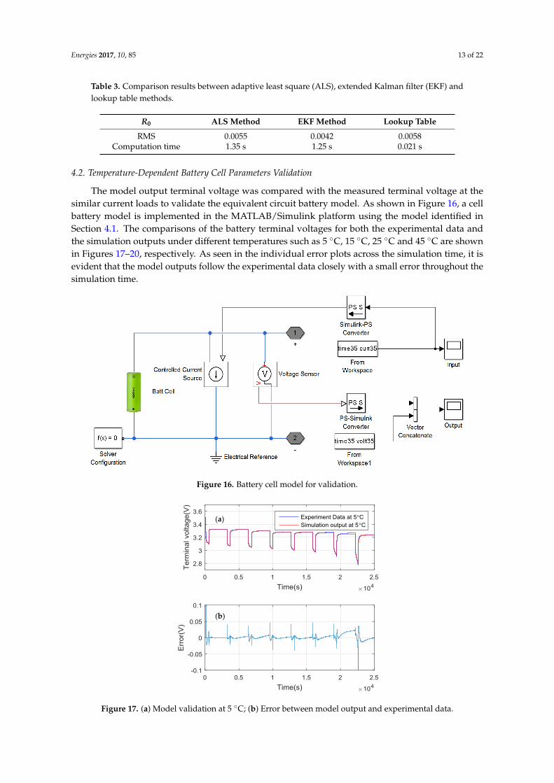
The model output terminal voltage was compared with the measured terminal voltage at thesimilar current loads to validate the equivalent circuit battery model. As shown in Figure 16, a cellbattery model is implemented in the MATLAB/Simulink platform using the model identified inSection 4.1. The comparisons of the battery terminal voltages for both the experimental data andthe simulation outputs under different temperatures such as 5 ◦C, 15 ◦C, 25 ◦C and 45 ◦C are shownin Figures 17–20, respectively. As seen in the individual error plots across the simulation time, it isevident that the model outputs follow the experimental data closely with a small error throughout thesimulation time.
Energies 2017, 10, 85 13 of 22
Table 3. Comparison results between adaptive least square (ALS), extended Kalman filter (EKF) and lookup table methods.
R0 ALS Method EKF Method Lookup Table RMS 0.0055 0.0042 0.0058
Computation time 1.35 s 1.25 s 0.021 s
4.2. Temperature-Dependent Battery Cell Parameters Validation
The model output terminal voltage was compared with the measured terminal voltage at the similar current loads to validate the equivalent circuit battery model. As shown in Figure 16, a cell battery model is implemented in the MATLAB/Simulink platform using the model identified in Section 4.1. The comparisons of the battery terminal voltages for both the experimental data and the simulation outputs under different temperatures such as 5 °C, 15 °C, 25 °C and 45 °C are shown in Figures 17–20, respectively. As seen in the individual error plots across the simulation time, it is evident that the model outputs follow the experimental data closely with a small error throughout the simulation time.
Figure 16. Battery cell model for validation.
Figure 17. (a) Model validation at 5 °C; (b) Error between model output and experimental data.
(a)
(b)
Figure 16. Battery cell model for validation.
Energies 2017, 10, 85 13 of 22
Table 3. Comparison results between adaptive least square (ALS), extended Kalman filter (EKF) and
lookup table methods.
R0 ALS Method EKF Method Lookup Table
RMS 0.0055 0.0042 0.0058
Computation time 1.35 s 1.25 s 0.021 s
4.2. Temperature-Dependent Battery Cell Parameters Validation
The model output terminal voltage was compared with the measured terminal voltage at the
similar current loads to validate the equivalent circuit battery model. As shown in Figure 16, a cell
battery model is implemented in the MATLAB/Simulink platform using the model identified in
Section 4.1. The comparisons of the battery terminal voltages for both the experimental data and the
simulation outputs under different temperatures such as 5 °C, 15 °C, 25 °C and 45 °C are shown in
Figures 17–20, respectively. As seen in the individual error plots across the simulation time, it is
evident that the model outputs follow the experimental data closely with a small error throughout
the simulation time.
Figure 16. Battery cell model for validation.
Figure 17. (a) Model validation at 5 °C; (b) Error between model output and experimental data.
(a)
(b)
Figure 17. (a) Model validation at 5 ◦C; (b) Error between model output and experimental data.
Energies 2017, 10, 85 14 of 22Energies 2017, 10, 85 14 of 22
Figure 18. (a) Model validation at 15 °C; (b) Error between model output and experimental data.
Figure 19. (a) Model validation at 25 °C; (b) Error between model output and experimental data.
For comparison purposes, the root means square errors of the terminal voltage between the
simulation and experimental results shown in Figures 17–20 at different temperatures are tabulated
in Table 4. The comparison between the simulation and experiment at various temperatures shows a
maximum RMS error of 7.2078 × 10⁻⁵. It shows the battery cell indeed operating quite poorly at a
lower temperature (a common characteristic of a battery cell). From the figures, it is evident that the
terminal voltage errors due to the suddenly changed current can be converged to around 0 quickly
(e.g., within 1.2 × 10⁻⁵ s); this means the model has a certain degree of robustness, which is relevant
to the further study of the advanced algorithms. To test the robustness of the model under different
ambient temperatures, a set of experimental data under 35 °C (not used for the parameter
(a)
(b)
(a)
(b)
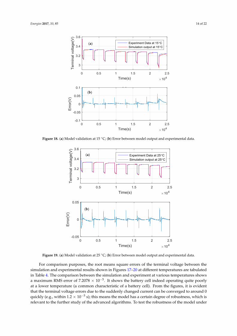
Figure 18. (a) Model validation at 15 ◦C; (b) Error between model output and experimental data.
Energies 2017, 10, 85 14 of 22
Figure 18. (a) Model validation at 15 °C; (b) Error between model output and experimental data.
Figure 19. (a) Model validation at 25 °C; (b) Error between model output and experimental data.
For comparison purposes, the root means square errors of the terminal voltage between the
simulation and experimental results shown in Figures 17–20 at different temperatures are tabulated
in Table 4. The comparison between the simulation and experiment at various temperatures shows a
maximum RMS error of 7.2078 × 10⁻⁵. It shows the battery cell indeed operating quite poorly at a
lower temperature (a common characteristic of a battery cell). From the figures, it is evident that the
terminal voltage errors due to the suddenly changed current can be converged to around 0 quickly
(e.g., within 1.2 × 10⁻⁵ s); this means the model has a certain degree of robustness, which is relevant
to the further study of the advanced algorithms. To test the robustness of the model under different
ambient temperatures, a set of experimental data under 35 °C (not used for the parameter
(a)
(b)
(a)
(b)
Figure 19. (a) Model validation at 25 ◦C; (b) Error between model output and experimental data.
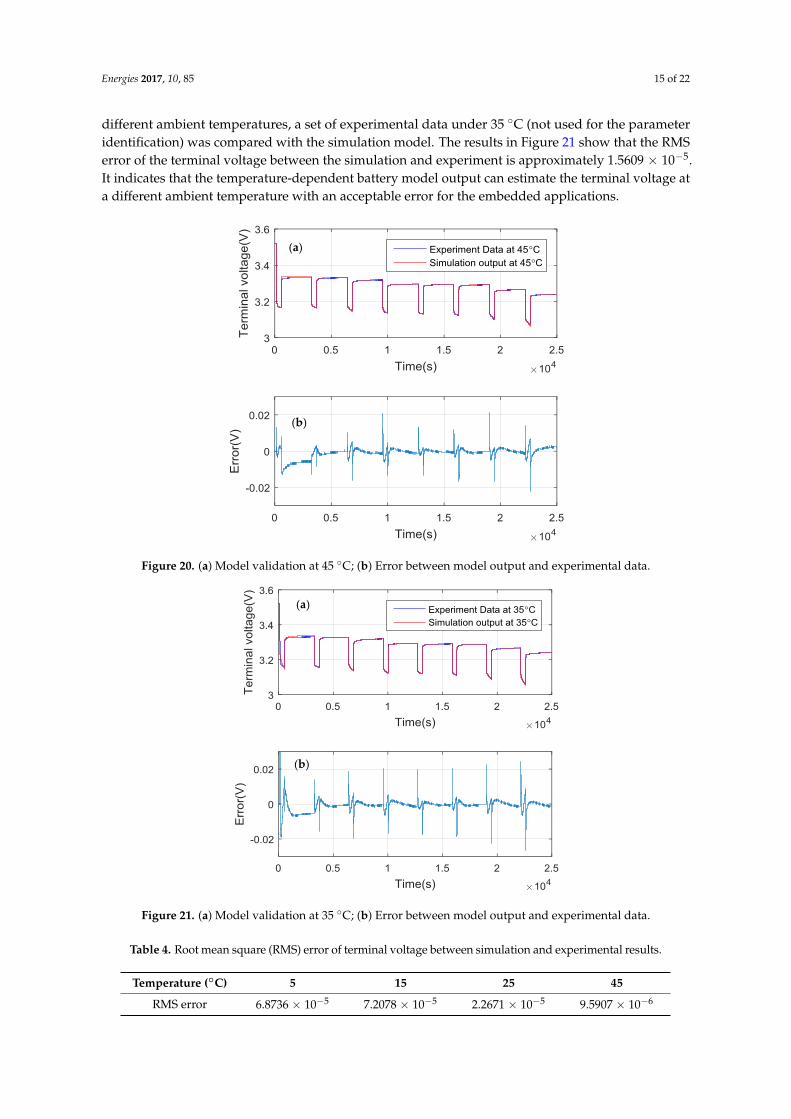
For comparison purposes, the root means square errors of the terminal voltage between thesimulation and experimental results shown in Figures 17–20 at different temperatures are tabulatedin Table 4. The comparison between the simulation and experiment at various temperatures showsa maximum RMS error of 7.2078 × 10⁻⁵. It shows the battery cell indeed operating quite poorlyat a lower temperature (a common characteristic of a battery cell). From the figures, it is evidentthat the terminal voltage errors due to the suddenly changed current can be converged to around 0quickly (e.g., within 1.2 × 10⁻⁵ s); this means the model has a certain degree of robustness, which isrelevant to the further study of the advanced algorithms. To test the robustness of the model under
Energies 2017, 10, 85 15 of 22
different ambient temperatures, a set of experimental data under 35 ◦C (not used for the parameteridentification) was compared with the simulation model. The results in Figure 21 show that the RMSerror of the terminal voltage between the simulation and experiment is approximately 1.5609 × 10⁻⁵.It indicates that the temperature-dependent battery model output can estimate the terminal voltage ata different ambient temperature with an acceptable error for the embedded applications.
Energies 2017, 10, 85 15 of 22
identification) was compared with the simulation model. The results in Figure 21 show that the RMS
error of the terminal voltage between the simulation and experiment is approximately 1.5609 × 10⁻⁵.
It indicates that the temperature-dependent battery model output can estimate the terminal voltage
at a different ambient temperature with an acceptable error for the embedded applications.
Figure 20. (a) Model validation at 45 °C; (b) Error between model output and experimental data.
Figure 21. (a) Model validation at 35 °C; (b) Error between model output and experimental data.
Table 4. Root mean square (RMS) error of terminal voltage between simulation and experimental
results.
Temperature (°C) 5 15 25 45
RMS error 6.8736 × 10⁻⁵ 7.2078 × 10⁻⁵ 2.2671 × 10⁻⁵ 9.5907 × 10⁻⁶
4.3. Temperature-Dependent 12-Cell Battery Model with Convective Heat Transfer Simulation
(a)
(b)
(a)
(b)
Figure 20. (a) Model validation at 45 ◦C; (b) Error between model output and experimental data.
Energies 2017, 10, 85 15 of 22
identification) was compared with the simulation model. The results in Figure 21 show that the RMS
error of the terminal voltage between the simulation and experiment is approximately 1.5609 × 10⁻⁵.
It indicates that the temperature-dependent battery model output can estimate the terminal voltage
at a different ambient temperature with an acceptable error for the embedded applications.
Figure 20. (a) Model validation at 45 °C; (b) Error between model output and experimental data.
Figure 21. (a) Model validation at 35 °C; (b) Error between model output and experimental data.
Table 4. Root mean square (RMS) error of terminal voltage between simulation and experimental
results.
Temperature (°C) 5 15 25 45
RMS error 6.8736 × 10⁻⁵ 7.2078 × 10⁻⁵ 2.2671 × 10⁻⁵ 9.5907 × 10⁻⁶
4.3. Temperature-Dependent 12-Cell Battery Model with Convective Heat Transfer Simulation
(a)
(b)
(a)
(b)
Figure 21. (a) Model validation at 35 ◦C; (b) Error between model output and experimental data.
Table 4. Root mean square (RMS) error of terminal voltage between simulation and experimental results.
Temperature (◦C) 5 15 25 45
RMS error 6.8736 × 10⁻⁵ 7.2078 × 10⁻⁵ 2.2671 × 10⁻⁵ 9.5907 × 10⁻⁶
Energies 2017, 10, 85 16 of 22
4.3. Temperature-Dependent 12-Cell Battery Model with Convective Heat Transfer Simulation
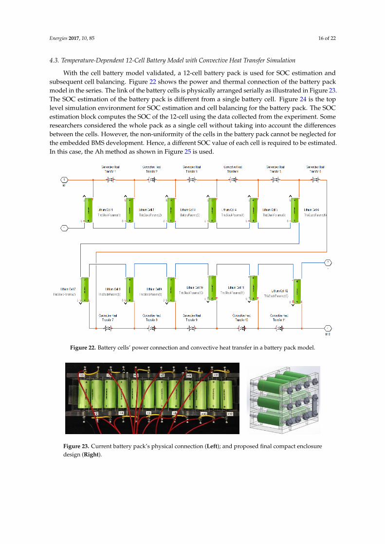
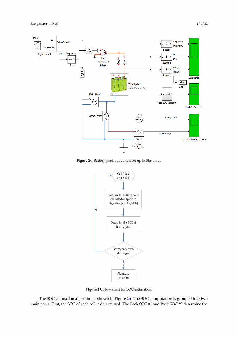
With the cell battery model validated, a 12-cell battery pack is used for SOC estimation andsubsequent cell balancing. Figure 22 shows the power and thermal connection of the battery packmodel in the series. The link of the battery cells is physically arranged serially as illustrated in Figure 23.The SOC estimation of the battery pack is different from a single battery cell. Figure 24 is the toplevel simulation environment for SOC estimation and cell balancing for the battery pack. The SOCestimation block computes the SOC of the 12-cell using the data collected from the experiment. Someresearchers considered the whole pack as a single cell without taking into account the differencesbetween the cells. However, the non-uniformity of the cells in the battery pack cannot be neglected forthe embedded BMS development. Hence, a different SOC value of each cell is required to be estimated.In this case, the Ah method as shown in Figure 25 is used.
Energies 2017, 10, 85 16 of 22
With the cell battery model validated, a 12-cell battery pack is used for SOC estimation and subsequent cell balancing. Figure 22 shows the power and thermal connection of the battery pack model in the series. The link of the battery cells is physically arranged serially as illustrated in Figure 23. The SOC estimation of the battery pack is different from a single battery cell. Figure 24 is the top level simulation environment for SOC estimation and cell balancing for the battery pack. The SOC estimation block computes the SOC of the 12-cell using the data collected from the experiment. Some researchers considered the whole pack as a single cell without taking into account the differences between the cells. However, the non-uniformity of the cells in the battery pack cannot be neglected for the embedded BMS development. Hence, a different SOC value of each cell is required to be estimated. In this case, the Ah method as shown in Figure 25 is used.
Figure 22. Battery cells’ power connection and convective heat transfer in a battery pack model.
Figure 23. Current battery pack’s physical connection (Left); and proposed final compact enclosure design (Right).
Figure 22. Battery cells’ power connection and convective heat transfer in a battery pack model.
Energies 2017, 10, 85 16 of 22
With the cell battery model validated, a 12-cell battery pack is used for SOC estimation and
subsequent cell balancing. Figure 22 shows the power and thermal connection of the battery pack
model in the series. The link of the battery cells is physically arranged serially as illustrated in Figure
23. The SOC estimation of the battery pack is different from a single battery cell. Figure 24 is the top
level simulation environment for SOC estimation and cell balancing for the battery pack. The SOC
estimation block computes the SOC of the 12-cell using the data collected from the experiment. Some
researchers considered the whole pack as a single cell without taking into account the differences
between the cells. However, the non-uniformity of the cells in the battery pack cannot be neglected
for the embedded BMS development. Hence, a different SOC value of each cell is required to be
estimated. In this case, the Ah method as shown in Figure 25 is used.
Figure 22. Battery cells’ power connection and convective heat transfer in a battery pack model.
Figure 23. Current battery pack’s physical connection (Left); and proposed final compact enclosure
design (Right). Figure 23. Current battery pack’s physical connection (Left); and proposed final compact enclosuredesign (Right).
Energies 2017, 10, 85 17 of 22Energies 2017, 10, 85 17 of 22
Figure 24. Battery pack validation set up in Simulink.
Figure 25. Flow chart for SOC estimation.
The SOC estimation algorithm is shown in Figure 26. The SOC computation is grouped into two main parts. First, the SOC of each cell is determined. The Pack SOC #1 and Pack SOC #2 determine the minimum SOC and the average SOC, respectively. The battery cell is checked for any over-
Figure 24. Battery pack validation set up in Simulink.
Energies 2017, 10, 85 17 of 22
Figure 24. Battery pack validation set up in Simulink.
Cells’ data
acquisition
Alarm and
protection
Battery pack over-
discharge?
Y
N
Calculate the SOC of every
cell based on specified
algorithm (e.g. Ah, EKF)
Determine the SOC of
battery pack
Figure 25. Flow chart for SOC estimation.
The SOC estimation algorithm is shown in Figure 26. The SOC computation is grouped into two
main parts. First, the SOC of each cell is determined. The Pack SOC #1 and Pack SOC #2 determine
the minimum SOC and the average SOC, respectively. The battery cell is checked for any over-
Figure 25. Flow chart for SOC estimation.
The SOC estimation algorithm is shown in Figure 26. The SOC computation is grouped into twomain parts. First, the SOC of each cell is determined. The Pack SOC #1 and Pack SOC #2 determine the

Energies 2017, 10, 85 18 of 22
minimum SOC and the average SOC, respectively. The battery cell is checked for any over-chargingbefore it sends out an alarm or warning signal. The SOC estimation algorithm also gives additionalSOC information for the subsequent cell balancing algorithm to prioritize the cell that needs to balancefirst. In this case, it should be the cell with the lowest SOC.
Energies 2017, 10, 85 18 of 22
charging before it sends out an alarm or warning signal. The SOC estimation algorithm also gives
additional SOC information for the subsequent cell balancing algorithm to prioritize the cell that
needs to balance first. In this case, it should be the cell with the lowest SOC.
Figure 26. (a) Current pulse; (b) simulation battery pack SOC result for battery pack SOC.
Since the SOC in each cell can be different, the cells need to be checked for over-charging and
balanced to operate for a longer endurance in embedded applications. Hence, the cell balancing
becomes an indispensable feature for real embedded BMS as it affects the lifespan and eventual safety
of the battery power system. Different types of model-based cell balancing algorithms can be
developed and validated in the MATLAB/Simulink environment using the battery pack model. For
clarity, only the battery cells #1 to #4 of the battery pack are used for comparison. Cells #1 and #2 are
employed for the passive balancing due to its simplicity and reliable performance. Cells #3 and #4 are
not used for any balancing function as shown in Figure 27. Instead, it is used to compare the cell
balancing results with cells #1 and #2 (that are not balanced). The balancing scheme is solely based
on average voltage. If the cell is not equal to the mean voltage, the cell balancing will begin to increase
the SOC. To do that, the SOC in each cell provides an input variable to the balancing decision block
(named “cell balancing block”). The initial SOC values of cells #1 to #4 are pre-set to 100%, 96%, 92%
and 81%, respectively, to show different initial SOV values. The simulation result (without the cell
balancing) is provided in Figure 28. The results indicate that battery cells with different initial states
will lead to different terminal voltages, SOC distributions, and thermal behaviors. As shown in Figure
29, cells #1 and #2 after cell balancing can maintain the SOC across each cell, and the SOC across all
the cells have improved by approximately 60% as compared to the one without the cell balancing.
Figure 26. (a) Current pulse; (b) simulation battery pack SOC result for battery pack SOC.
Since the SOC in each cell can be different, the cells need to be checked for over-charging andbalanced to operate for a longer endurance in embedded applications. Hence, the cell balancingbecomes an indispensable feature for real embedded BMS as it affects the lifespan and eventualsafety of the battery power system. Different types of model-based cell balancing algorithms can bedeveloped and validated in the MATLAB/Simulink environment using the battery pack model. Forclarity, only the battery cells #1 to #4 of the battery pack are used for comparison. Cells #1 and #2 areemployed for the passive balancing due to its simplicity and reliable performance. Cells #3 and #4are not used for any balancing function as shown in Figure 27. Instead, it is used to compare the cellbalancing results with cells #1 and #2 (that are not balanced). The balancing scheme is solely based onaverage voltage. If the cell is not equal to the mean voltage, the cell balancing will begin to increase theSOC. To do that, the SOC in each cell provides an input variable to the balancing decision block (named“cell balancing block”). The initial SOC values of cells #1 to #4 are pre-set to 100%, 96%, 92% and 81%,respectively, to show different initial SOV values. The simulation result (without the cell balancing) isprovided in Figure 28. The results indicate that battery cells with different initial states will lead todifferent terminal voltages, SOC distributions, and thermal behaviors. As shown in Figure 29, cells #1and #2 after cell balancing can maintain the SOC across each cell, and the SOC across all the cells haveimproved by approximately 60% as compared to the one without the cell balancing.

Energies 2017, 10, 85 19 of 22Energies 2017, 10, x FOR PEER REVIEW 19 of 22
Figure 27. Cell balancing algorithm development in Simulink (for clarity only show 5-cell).
Figure 27. Cell balancing algorithm development in Simulink (for clarity only show 5-cell).

Energies 2017, 10, 85 20 of 22Energies 2017, 10, x FOR PEER REVIEW 20 of 22
Figure 28. Battery pack simulation result without cell balancing: (a) current pulse (active when
charging and negative when discharging); (b) voltage response of each cell; (c) SOC of each cell; (d)
temperature of each cell.
Figure 29. Simulation result with cell balancing: (a) comparison of cell #1 to #4; (b) error between cell
voltage and average voltage of cell #1 to #4 after balancing.
In summary, the proposed battery pack model can estimate the SOC of each cell and temperature
between the cells. The passive cell balancing scheme was applied on the temperature-dependent
battery model. Although the active balancing system has attracted more attention as of late, it is quite
Figure 28. Battery pack simulation result without cell balancing: (a) current pulse (active when chargingand negative when discharging); (b) voltage response of each cell; (c) SOC of each cell; (d) temperatureof each cell.
Energies 2017, 10, x FOR PEER REVIEW 20 of 22
Figure 28. Battery pack simulation result without cell balancing: (a) current pulse (active when
charging and negative when discharging); (b) voltage response of each cell; (c) SOC of each cell; (d)
temperature of each cell.
Figure 29. Simulation result with cell balancing: (a) comparison of cell #1 to #4; (b) error between cell
voltage and average voltage of cell #1 to #4 after balancing.
In summary, the proposed battery pack model can estimate the SOC of each cell and temperature
between the cells. The passive cell balancing scheme was applied on the temperature-dependent
battery model. Although the active balancing system has attracted more attention as of late, it is quite
Figure 29. Simulation result with cell balancing: (a) comparison of cell #1 to #4; (b) error between cellvoltage and average voltage of cell #1 to #4 after balancing.
In summary, the proposed battery pack model can estimate the SOC of each cell and temperaturebetween the cells. The passive cell balancing scheme was applied on the temperature-dependent

Energies 2017, 10, 85 21 of 22
battery model. Although the active balancing system has attracted more attention as of late, it is quitecostly, possesses a sophisticated control structure and requires higher power consumption than passivecell balancing.
5. Conclusions
In this paper, a simple but effective battery model was proposed, which was suitable to beimplemented in a microcontroller with limited resources for the embedded applications. Simplifiedlookup table with interpolation technique is applied to obtain the real-time open-circuit voltage (OCV),R1 and C1, which is a highly efficient method for the microcontroller implementation in the embeddedapplications. Furthermore, based on the proposed cell model, a 12-cell series connected battery pack issystematically modeled, simulated and validated by actual experimental results. This paper mainlyfocused on the 12-cell LiFePO4 battery pack for a more realistic simulation instead of a single batterycell. As a trade-off between the high fidelity and computation effort, the conductive thermal transferis neglected in this paper. Instead of using the temperature as an external disturbance acting on thebattery power system, the thermal influence due to convective heat transfer of each cell was includedas parameters to couple both the equivalent circuit model (ECM) and the thermal model. Also, thetemperature-dependent battery model was included to estimate the SOC that was balanced by anautomatic cell balancing scheme. As compared with the experimental results, there exists a minimalroot mean square error of the terminal voltage at a different ambient temperature (from 5 ◦C to 45 ◦C).The proposed simulation model allows SOC and temperature estimation of the battery cells for theembedded implementation. It can be used to develop and validate any advanced algorithms using theproposed battery cell/pack model.
For future works, the high current rate and effects of aging will be included. More experimentalworks will be conducted. The fault diagnosis approach will be performed on the final battery model.The mechanical enclosure will be used to hold the battery pack.
Acknowledgments: This work was supported by Singapore Maritime Institute (SMI) through the project(SMI-2013-MA-05). The authors would like to thank Newcastle University, Mahesh Menon and John McCannfrom Soil Machine Dynamics (SMD) Ltd and Cham Yew Thean from Temasek Polytechnic for providingresearch supports.
Author Contributions: Zuchang Gao is credited with the majority of the theoretical formulation, simulation andexperimental works performed in this paper for his Ph.D. study and project involvement under SMI-2013-MA-05.Cheng Siong Chin who is the main supervisor defined the flow of the paper and participated in the battery powersystem simulation and verification that drove this research with Wai Lok Woo and Junbo Jia to test its relevancefor industrial applications. Wai Lok Woo and Junbo Jia provided the co-supervision and academic support duringthe project. All authors discussed and provided comments on the results at all stages to the final proofreading.
Conflicts of Interest: The authors declare no conflict of interest.
References
1. Chang, M.-H.; Huang, H.-P.; Chang, S.-W. A new state of charge estimation method for LiFePO4 batterypacks used in robots. Energies 2013, 6, 2007–2030. [CrossRef]
2. Alhanouti, M.; Gießler, M.; Blank, T.; Gauterin, F. New electro-thermal battery pack model of an electricvehicle. Energies 2016, 9. [CrossRef]
3. Zhang, C.; Li, K.; Pei, L.; Zhu, C. An integrated approach for real-time model-based state-of-charge estimationof lithium-ion batteries. J. Power Sources 2015, 283, 24–36. [CrossRef]
4. Awadallah, M.A.; Venkatesh, B. Accuracy improvement of Soc estimation in lithium-ion batteries. J. EnergyStorage 2016, 6, 95–104. [CrossRef]
5. Hansen, T.; Wang, C.-J. Support vector based battery state of charge estimator. J. Power Sources 2005, 141,351–358. [CrossRef]
6. Chaoui, H.; Golbon, N.; Hmouz, I.; Souissi, R.; Tahar, S. Lyapunov-based adaptive state of charge and stateof health estimation for lithium-ion batteries. IEEE Trans. Ind. Electron. 2015, 62, 1610–1618. [CrossRef]

Energies 2017, 10, 85 22 of 22
7. Gandolfo, D.; Brandão, A.; Patiño, D.; Molina, M. Dynamic model of lithium polymer battery—Load resistormethod for electric parameters identification. J. Energy Inst. 2015, 88, 470–479. [CrossRef]
8. Lee, J.L.; Chemistruck, A.; Plett, G.L. Discrete-time realization of transcendental impedance models, withapplication to modeling spherical solid diffusion. J. Power Sources 2012, 206, 367–377. [CrossRef]
9. Coleman, M.; Lee, C.K.; Zhu, C.; Hurley, W.G. State-of-charge determination from emf voltage estimation:Using impedance, terminal voltage, and current for lead-acid and lithium-ion batteries. IEEE Trans.Ind. Electron. 2007, 54, 2550–2557. [CrossRef]
10. Hussein, A.A. Capacity fade estimation in electric vehicle Li-ion batteries using artificial neural networks.IEEE Trans. Ind. Appl. 2015, 51, 2321–2330. [CrossRef]
11. Li, I.H.; Wang, W.Y.; Su, S.F.; Lee, Y.S. A merged fuzzy neural network and its applications in batterystate-of-charge estimation. IEEE Trans. Energy Convers. 2007, 22, 697–708. [CrossRef]
12. Charkhgard, M.; Farrokhi, M. State-of-charge estimation for lithium-ion batteries using neural networksand ekf. IEEE Trans. Ind. Electron. 2010, 57, 4178–4187. [CrossRef]
13. Gao, Z.; Chin, C.S.; Woo, W.L.; Jia, J.; Toh, W.D. Lithium-ion battery modeling and validation for smartpower system. In Proceedings of the 2015 International Conference on Computer, Communications, andControl Technology (I4CT), Kuching, Malaysia, 21–23 April 2015; pp. 269–274.
14. Liu, S.; Jiang, J.; Shi, W.; Ma, Z.; Wang, L.Y.; Guo, H. Butler–volmer-equation-based electrical model forhigh-power lithium titanate batteries used in electric vehicles. IEEE Trans. Ind. Electron. 2015, 62, 7557–7568.[CrossRef]
15. Melin, P.; Castillo, O. Intelligent control of complex electrochemical systems with a neuro-fuzzy-geneticapproach. IEEE Trans. Ind. Electron. 2001, 48, 951–955. [CrossRef]
16. Lin, H.T.; Liang, T.J.; Chen, S.M. Estimation of battery state of health using the probabilistic neural network.IEEE Trans. Ind. Inform. 2013, 9, 679–685. [CrossRef]
17. Wang, S.C.; Liu, Y.H. A pso-based fuzzy-controlled searching for the optimal charge pattern of Li-ionbatteries. IEEE Trans. Ind. Electron. 2015, 62, 2983–2993. [CrossRef]
18. Kim, J.; Cho, B.H. State-of-charge estimation and state-of-health prediction of a Li-ion degraded batterybased on an ekf combined with a per-unit system. IEEE Trans. Veh. Technol. 2011, 60, 4249–4260. [CrossRef]
19. He, W.; Williard, N.; Chen, C.; Pecht, M. State of charge estimation for Li-ion batteries using neural networkmodeling and unscented Kalman filter-based error cancellation. Int. J. Electr. Power Energy Syst. 2014, 62,783–791. [CrossRef]
20. Partovibakhsh, M.; Liu, G. An adaptive unscented Kalman filtering approach for online estimation of modelparameters and state-of-charge of lithium-ion batteries for autonomous mobile robots. IEEE Trans. ControlSyst. Technol. 2015, 23, 357–363. [CrossRef]
© 2017 by the authors; licensee MDPI, Basel, Switzerland. This article is an open accessarticle distributed under the terms and conditions of the Creative Commons Attribution(CC-BY) license (http://creativecommons.org/licenses/by/4.0/).