Integrated Control and Real­Time Scheduling

Integrated Control andReal­Time Scheduling

Anton Cervin

Department of Automatic Control

Lund Institute of Technology

Lund, April 2003

Department of Automatic ControlLund Institute of TechnologyBox 118SE-221 00 LUNDSweden

ISSN 0280–5316ISRN LUTFD2/TFRT--1065--SE

c© 2003 by Anton Cervin. All rights reserved.Printed in Sweden by Bloms i Lund Tryckeri AB.Lund 2003

Abstract

The topic of the thesis is codesign of flexible real­time control systems.Integrating control theory and real­time scheduling theory, it is possibleto achieve higher resource utilization and better control performance. Theintegration requires new tools for analysis, design, and implementation.The problem of scheduling the individual parts of a control algorithm is

studied. It is shown how subtask scheduling can reduce the input­outputlatency in a set of control tasks. Deadline assignment under differentscheduling policies is considered.A feedback scheduling architecture for control tasks is introduced. The

scheduler uses feedback from execution­time measurements and feedfor­ward from workload changes to adjust the sampling periods of a set ofcontrol tasks so that the combined performance of the controllers is opti­mized.The Control Server, a novel computational model for real­time control

tasks, is presented. The model combines time­triggered I/O with dynamic,reservation­based task scheduling. The model provides short input­outputlatencies and minimal jitter for the controllers. It also allows control tasksto be treated as scalable real­time components with predictable perfor­mance.Two MATLAB­based toolboxes for analysis and simulation of real­time

control systems have been developed. The Jitterbug toolbox evaluates aquadratic cost function for a linear control system with timing variations.The tool makes it possible to investigate the impact of delay, jitter, lostsamples, etc., on control performance. The TrueTime toolbox facilitates de­tailed cosimulation of distributed real­time control systems. The schedul­ing and execution of control tasks is simulated in parallel with the net­work communication and the continuous process dynamics.

5

Acknowledgments

First, I would like to thank my supervisor Karl­Erik Årzén. He, togetherwith Klas Nilsson and Ola Dahl, wrote the original proposal for the re­search project “Integrated Control and Scheduling”. Never short on goodideas, Karl­Erik has been an excellent advisor since the day I started mygraduate studies. He has also been a constant supplier of good music overthe years.This thesis would not have turned out half as good without the help

from several of my fellow PhD students and colleagues. Johan Eker isthe co­author of a staggering 50% of my publications. Together, we haveworked on the simulator, feedback scheduling, and, most recently, the Con­trol Server. Dan Henriksson has been the main implementer of the newversion of the simulator, called TrueTime. Bo Lincoln has implementedthe Jitterbug analysis toolbox. Thank you all for the great work!It has been wonderful to work at the Department of Automatic Control

in Lund, where the people are always friendly and helpful. The professors,the secretaries, and the technical staff keep the department running verysmoothly. I would especially like to thank the founder of the department,Karl Johan Åström, who lured me into the field of automatic control andencouraged me to become a PhD student. Also, I would like to thank myco­supervisors Bo Bernhardsson and Per Hagander.During my studies, I have had the opportunity to visit colleagues

abroad. I would like to thank Professor Lui Sha at the Department ofComputer Science, University of Illinois at Urbana­Champaign for muchinspiration and visits on two separate occasions. I would also like to thankProfessor Edward Lee at the Department of Electrical Engineering andComputer Sciences, University of California at Berkeley for a researchvisit in 2001.This research project has been a collaboration between the Department

of Automatic Control and the Department of Computer Science at LundInstitute of Technology. It has been a pleasure to work together with Klas

7

Acknowledgments

Nilsson, Patrik Persson, and Sven Gestegård Robertz.The work in this thesis has been supported by ARTES, a real­time

research network in Sweden funded by SSF. I have enjoyed visits to sev­eral summer schools, graduate student conferences, and other activitiesorganized by ARTES over the past five years.ARTES has provided funding for several conference trips and research

visits. A travel grant from the Royal Physiographic Society in Lund is alsogratefully acknowledged.Finally, I would like thank my family, friends, fellow lindy hoppers,

poker buddies, etc., for making my life so enjoyable! A special thank yougoes out to Matilda for her love and inspiration.

Anton

8

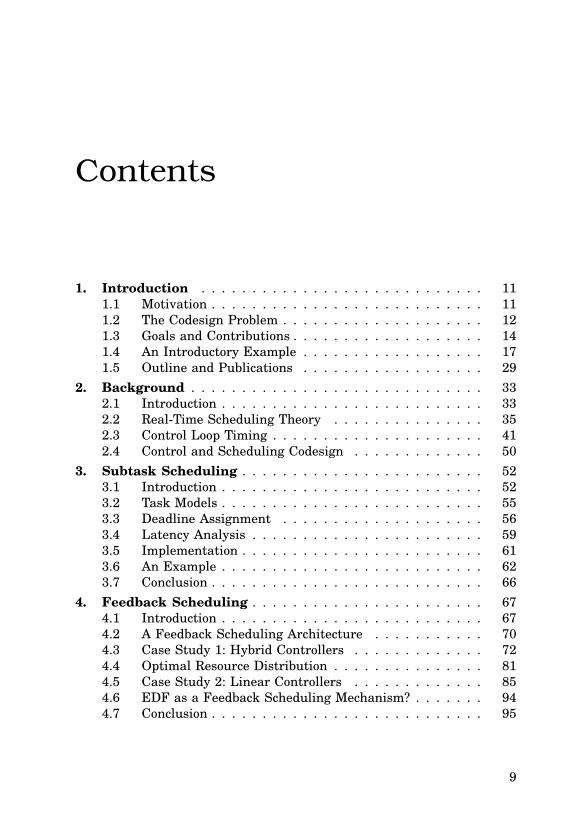
Contents

1. Introduction . . . . . . . . . . . . . . . . . . . . . . . . . . . . 111.1 Motivation . . . . . . . . . . . . . . . . . . . . . . . . . . . 111.2 The Codesign Problem . . . . . . . . . . . . . . . . . . . . 121.3 Goals and Contributions . . . . . . . . . . . . . . . . . . . 141.4 An Introductory Example . . . . . . . . . . . . . . . . . . 171.5 Outline and Publications . . . . . . . . . . . . . . . . . . 29

2. Background . . . . . . . . . . . . . . . . . . . . . . . . . . . . . 332.1 Introduction . . . . . . . . . . . . . . . . . . . . . . . . . . 332.2 Real­Time Scheduling Theory . . . . . . . . . . . . . . . 352.3 Control Loop Timing . . . . . . . . . . . . . . . . . . . . . 412.4 Control and Scheduling Codesign . . . . . . . . . . . . . 50

3. Subtask Scheduling . . . . . . . . . . . . . . . . . . . . . . . . 523.1 Introduction . . . . . . . . . . . . . . . . . . . . . . . . . . 523.2 Task Models . . . . . . . . . . . . . . . . . . . . . . . . . . 553.3 Deadline Assignment . . . . . . . . . . . . . . . . . . . . 563.4 Latency Analysis . . . . . . . . . . . . . . . . . . . . . . . 593.5 Implementation . . . . . . . . . . . . . . . . . . . . . . . . 613.6 An Example . . . . . . . . . . . . . . . . . . . . . . . . . . 623.7 Conclusion . . . . . . . . . . . . . . . . . . . . . . . . . . . 66

4. Feedback Scheduling . . . . . . . . . . . . . . . . . . . . . . . 674.1 Introduction . . . . . . . . . . . . . . . . . . . . . . . . . . 674.2 A Feedback Scheduling Architecture . . . . . . . . . . . 704.3 Case Study 1: Hybrid Controllers . . . . . . . . . . . . . 724.4 Optimal Resource Distribution . . . . . . . . . . . . . . . 814.5 Case Study 2: Linear Controllers . . . . . . . . . . . . . 854.6 EDF as a Feedback Scheduling Mechanism? . . . . . . . 944.7 Conclusion . . . . . . . . . . . . . . . . . . . . . . . . . . . 95

9

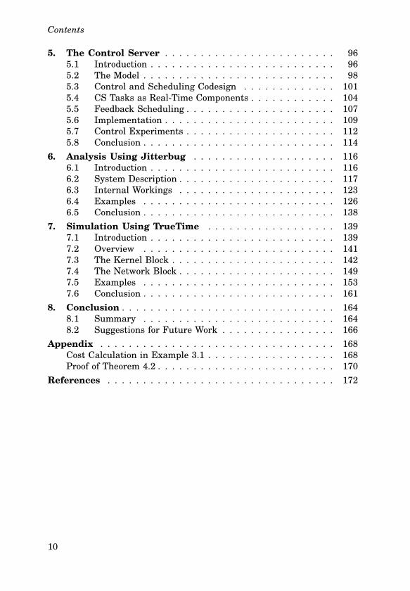
Contents

5. The Control Server . . . . . . . . . . . . . . . . . . . . . . . . 965.1 Introduction . . . . . . . . . . . . . . . . . . . . . . . . . . 965.2 The Model . . . . . . . . . . . . . . . . . . . . . . . . . . . 985.3 Control and Scheduling Codesign . . . . . . . . . . . . . 1015.4 CS Tasks as Real­Time Components . . . . . . . . . . . . 1045.5 Feedback Scheduling . . . . . . . . . . . . . . . . . . . . . 1075.6 Implementation . . . . . . . . . . . . . . . . . . . . . . . . 1095.7 Control Experiments . . . . . . . . . . . . . . . . . . . . . 1125.8 Conclusion . . . . . . . . . . . . . . . . . . . . . . . . . . . 114

6. Analysis Using Jitterbug . . . . . . . . . . . . . . . . . . . . 1166.1 Introduction . . . . . . . . . . . . . . . . . . . . . . . . . . 1166.2 System Description . . . . . . . . . . . . . . . . . . . . . . 1176.3 Internal Workings . . . . . . . . . . . . . . . . . . . . . . 1236.4 Examples . . . . . . . . . . . . . . . . . . . . . . . . . . . 1266.5 Conclusion . . . . . . . . . . . . . . . . . . . . . . . . . . . 138

7. Simulation Using TrueTime . . . . . . . . . . . . . . . . . . 1397.1 Introduction . . . . . . . . . . . . . . . . . . . . . . . . . . 1397.2 Overview . . . . . . . . . . . . . . . . . . . . . . . . . . . 1417.3 The Kernel Block . . . . . . . . . . . . . . . . . . . . . . . 1427.4 The Network Block . . . . . . . . . . . . . . . . . . . . . . 1497.5 Examples . . . . . . . . . . . . . . . . . . . . . . . . . . . 1537.6 Conclusion . . . . . . . . . . . . . . . . . . . . . . . . . . . 161

8. Conclusion . . . . . . . . . . . . . . . . . . . . . . . . . . . . . . 1648.1 Summary . . . . . . . . . . . . . . . . . . . . . . . . . . . 1648.2 Suggestions for Future Work . . . . . . . . . . . . . . . . 166

Appendix . . . . . . . . . . . . . . . . . . . . . . . . . . . . . . . . . 168Cost Calculation in Example 3.1 . . . . . . . . . . . . . . . . . . 168Proof of Theorem 4.2 . . . . . . . . . . . . . . . . . . . . . . . . . 170

References . . . . . . . . . . . . . . . . . . . . . . . . . . . . . . . . 172

10

1

Introduction

1.1 Motivation

Real­time control plays an important part in modern technology. For ex­ample, a CD or DVD player could never operate without its feedback con­trol system. Engine management systems in modern cars rely heavily onreal­time computations and feedback control to improve performance, re­duce fuel consumption, and minimize the amount of pollutant emissions.As the capacity of microcontrollers is increasing and the cost is decreasing,more and more functionality is realized in software. In an embedded con­trol system, a control task is typically executing in parallel with severalother tasks, including other control tasks. This puts focus on scheduling,i.e., the choice of which task to execute at a given time. Since the begin­ning of the 1970s, the academic interest in real­time scheduling has beenvery large. Very little of this work has, however, focused on control tasks.On the other hand, digital control theory, with its origin in the 1950s, doesnot address the problem of shared and limited resources in the computingsystem. Instead, it is commonly assumed that the controller executes asa simple loop in a dedicated computer.Real­time scheduling is sometimes dismissed as a non­problem. With

ever more powerful computers, it can be argued that most timing problemscan be solved by upgrading the CPU to a later and faster model. Whilethis might be true in some cases, developers of embedded systems willtestify that they are always struggling to add yet another function to analready heavily loaded processor. To keep production costs down, manufac­turers of consumer products tend, of course, to use the most inexpensivehardware possible. Only in extreme applications, such as nuclear powerplants, can the cost of the computing hardware be neglected in the overalldevelopment costs.

11

Introduction

This work aims at achieving the best possible control performancefrom limited computing resources. To accomplish this goal, integrationof the control design and the real­time scheduling design is necessary.Today, the design of a real­time control system is typically a two­step pro­cedure: control design followed by real­time design. Moreover, the stepsare often carried out in relative isolation and by engineers with differentbackgrounds. The control engineer designs and evaluates the control al­gorithms assuming a very simple model of the computing platform. Thecomputer scientist schedules the controllers together with other tasks andmakes design trade­offs without really knowing the controller timing re­quirements. The isolated development introduces conservatism and leadsto non­optimal solutions.There is a strong trend towards flexibility in real­time control. In the

past, developers have relied on static analysis and design, knowing thatthe controllers would execute on deterministic hardware and in a pre­dictable environment. Today, both hardware and operating systems tendto be commercial­off­the­shelf (COTS) products, sometimes poorly spec­ified, and typically optimized for high average­case performance ratherthan predictable worst­case performance. Controllers are more frequentlybeing treated as software components, expected to work in different con­figurations and being subject to on­line upgrades. Furthermore, moderncontrol systems are often distributed systems, where sensors, controllers,and actuators are located in different nodes in a network. A distributedsystem is more flexible in nature but also more nondeterministic. Com­munication protocols may introduce timing variations that influence boththe control performance and the task scheduling in the various computernodes.

1.2 The Codesign Problem

Successful development of a real­time control system requires codesignof the computer system and the control system. The computing platformmust be dimensioned such that all functionality can be accommodated,and the controllers must be designed taking the hardware limitations intoaccount. The computer system has many important aspects (numerics,memory, I/O, network, power consumption, etc.). This thesis focuses onthe scheduling of control tasks in the CPU.The control and scheduling codesign problem can be informally stated

as follows:

Given a set of processes to be controlled and a computer withlimited computational resources, design a set of controllers and

12

1.2 The Codesign Problem

schedule them as real­time tasks such that the overall controlperformance is optimized.

An alternative view of the same problem is to say that we should de­sign and schedule a set of controllers such that the least expensive im­plementation platform can be used while still meeting the performancespecifications.The nature and the degree of difficulty of the codesign problem for a

given system depend on a number of factors:

• The real­time operating system.What scheduling algorithms are sup­ported? How is I/O handled? Can the real­time kernel measure taskexecution times and detect execution overruns and missed dead­lines?

• The scheduling algorithm. Is is time­driven or event­driven, priority­driven or deadline­driven? What analytical results regarding schedu­lability and response times are available? How are task overrunshandled? What scheduling parameters can be changed on­line?

• The controller synthesis method. What design criteria are used? Arethe controllers designed in the continuous­time domain and thendiscretized or is direct discrete design used? Are the controllers de­signed to be robust against timing variations? Should they activelycompensate for timing variations?

• The execution­time characteristics of the control algorithms. Do thealgorithms have predictable worst­case execution times? Are therelarge variations in execution time from sample to sample? Do thecontrollers switch between different internal modes with differentexecution­time profiles?

• Off­line or on­line optimization. What information is available forthe off­line design and how accurate is it? What can be measured on­line? Should the system be able to handle the arrival of new tasks?Should the system be re­optimized when the workload changes?Should there be feedback from the control performance to the schedul­ing algorithm?

The problems studied in this thesis will assume a real­time operat­ing system that supports dynamic scheduling algorithms (fixed­priorityor earliest­deadline­first scheduling). We will mainly consider schedul­ing of linear controllers whose performance is evaluated by quadratic costfunctions. When on­line optimization is introduced, it will be assumed thatthe execution times of the tasks can be measured, and that the schedulingparameters can be changed on­line.

13

Introduction

1.3 Goals and Contributions

Control theory and real­time systems theory have evolved as separatefields during the last couple of decades. There is clearly a lack of commonunderstanding between the two research communities and no well­defineddesign interface. In the control community, the real­time system is viewedas a platform on which the controller can be trivially implemented. In thereal­time systems community, a controller is viewed as a piece of codecharacterized by three fixed parameters: a period, a computation time,and a deadline. This thesis aims at bridging the gap between the tworesearch areas. For this purpose, new tools and techniques for analysis,design, and implementation are needed. The goals and contributions ofthe thesis are outlined below.

New Analysis Tools

There is a need for better understanding of what happens when a con­troller is implemented and scheduled as a real­time task. For this purpose,two MATLAB­based analysis tools have been developed: TrueTime1 andJitterbug 2. The tools can be used at early design stages to determine howsensitive controllers are to scheduling­induced delays and jitter. They canalso be used at the implementation stage for trade­off analysis betweenthe tasks.TrueTime, which is based on MATLAB/Simulink, is used for detailed

co­simulation of the computer system and the control system. In thetool, time is added as a new dimension to the control algorithms. Thecontrollers are executed in a real­time operating system, which is simu­lated in parallel with the continuous­time plant dynamics. An arbitraryscheduling algorithm can be used, and the code can be simulated on atime­scale of choice. The tool is very general and can be used to investi­gate, for instance, the influence of various scheduling algorithms on thecontrol performance. Although it falls outside the main scope of this the­sis, TrueTime can also be used to simulate distributed control systems andevaluate different communication protocols from a control perspective.Simulation is a very useful tool for control systems design but there

are limitations. The user may lack exact knowledge of task executionin the target system. Also, very long simulation times may be neededto draw conclusions about performance and stability. As an alternative,Jitterbug can be used for analysis of simple models of real­time controlsystems. In the tool, the timing variations introduced by the real­timeoperating system are modeled by statistical delay distributions. Given a

1Available at http://www.control.lth.se/˜dan/truetime/2Available at http://www.control.lth.se/˜ lincoln/jitterbug/

14

1.3 Goals and Contributions

linear control system and a timing model, the tool analytically computesa quadratic performance index, or cost function. By evaluating the costfunction for a wide range of timing parameters, the designer can inves­tigate how sensitive the control loop is to timing variations. Jitterbugalso supports frequency­domain analysis in the form of spectral densitycalculations.

More Detailed Scheduling Analysis

For a given system, the analysis tools above may indicate that controllertiming is a critical issue. The implementation may introduce latency andjitter that deteriorate the performance and force the developer to use amore expensive CPU. It can then be valuable to perform a more detailedscheduling analysis in order to reduce the latencies. The remaining delaycan be compensated for using control theory.One way to reduce the input­output latency in a controller is to split

the control algorithm into two parts: Calculate Output and Update State.The Calculate Output part should only contain the operations necessaryto produce a control signal, while the rest of the operations should bepostponed to the Update State part. In the thesis, it is shown how the twoparts can be scheduled as subtasks in order to reduce the input­outputlatency for a set of controllers. The control performance improvementscome at the expense of a slightly more complex implementation.

Introduction of Feedback in the Computing System

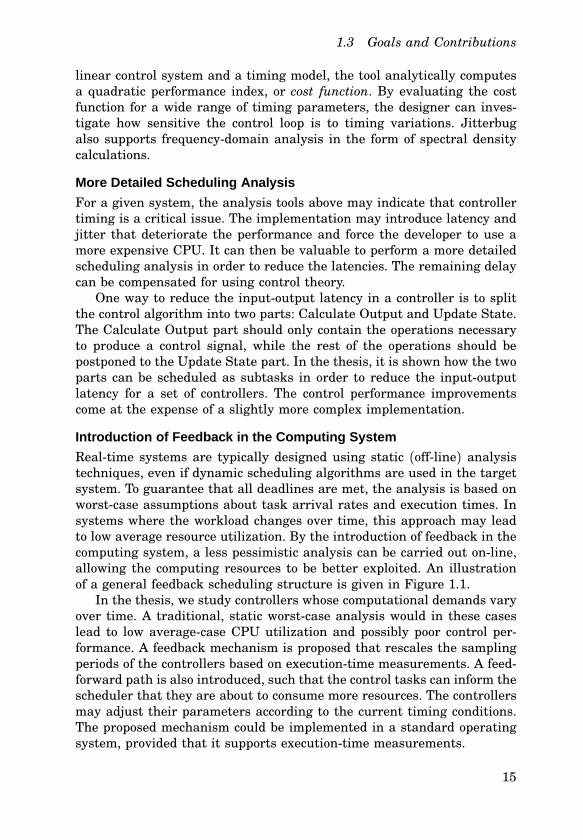
Real­time systems are typically designed using static (off­line) analysistechniques, even if dynamic scheduling algorithms are used in the targetsystem. To guarantee that all deadlines are met, the analysis is based onworst­case assumptions about task arrival rates and execution times. Insystems where the workload changes over time, this approach may leadto low average resource utilization. By the introduction of feedback in thecomputing system, a less pessimistic analysis can be carried out on­line,allowing the computing resources to be better exploited. An illustrationof a general feedback scheduling structure is given in Figure 1.1.In the thesis, we study controllers whose computational demands vary

over time. A traditional, static worst­case analysis would in these caseslead to low average­case CPU utilization and possibly poor control per­formance. A feedback mechanism is proposed that rescales the samplingperiods of the controllers based on execution­time measurements. A feed­forward path is also introduced, such that the control tasks can inform thescheduler that they are about to consume more resources. The controllersmay adjust their parameters according to the current timing conditions.The proposed mechanism could be implemented in a standard operatingsystem, provided that it supports execution­time measurements.

15

Introduction

Scheduler Tasks Resources

Feedforward

Feedback

Figure 1.1 A general feedback scheduling structure. The resources are distributedamong the tasks based on feedback from the actual resource use. The tasks can beuse feedforward to notify the scheduler about changes in their resource demands.

A Novel Computational Model

The scheduling techniques outlined above are mainly based on the fixed­priority scheduling algorithm, which is the standard scheduling mecha­nism in commercial real­time operating systems (RTOS). This algorithmhas several drawbacks, however, from both control and scheduling pointsof view. First, it introduces very irregular and hard­to­analyze delay pat­terns in the control loops. Second, the processor cannot be fully utilized,and the utilization bound depends on the task parameters in a non­trivialway. All of this makes for an extremely complicated control and schedul­ing codesign problem. In practice, the true performance of the controllercannot be known until it is running in the target system.To remedy this problem, we propose a novel computational model for

real­time control tasks, called the Control Server. The model assumes areal­time operating system that supports the earliest­deadline­first (EDF)scheduling algorithm, an optimal algorithm, which has yet to gain wide­spread use in commercial real­time operating systems. Interesting prop­erties of the model include small jitter, short input­output latencies, andisolation between unrelated tasks. A control task has a single adjustableparameter—the CPU utilization factor—that uniquely determines boththe control performance and the schedulability of the task. The utiliza­tion factor serves as a simple interface between the control design andthe real­time design.Controllers executing under the Control Server model can be viewed

as scalable real­time components with well­defined control and schedulingproperties. The model can ideally be combined with a feedback schedul­ing mechanism that optimizes the overall control performance as the sys­tem workload changes. The simple interface between the control and thescheduling design makes for a reasonably simple codesign problem to besolved on­line.

16

1.4 An Introductory Example

replacements

y1 y2 y3

u1 u2 u3

Figure 1.2 Three inverted pendulums should be stabilized using one computer.

1.4 An Introductory Example

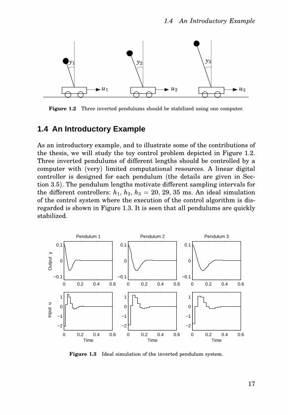
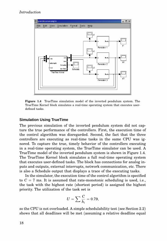
As an introductory example, and to illustrate some of the contributions ofthe thesis, we will study the toy control problem depicted in Figure 1.2.Three inverted pendulums of different lengths should be controlled by acomputer with (very) limited computational resources. A linear digitalcontroller is designed for each pendulum (the details are given in Sec­tion 3.5). The pendulum lengths motivate different sampling intervals forthe different controllers: h1, h2, h3 = 20, 29, 35 ms. An ideal simulationof the control system where the execution of the control algorithm is dis­regarded is shown in Figure 1.3. It is seen that all pendulums are quicklystabilized.

0 0.2 0.4 0.6

−0.1

0

0.1

Out

put

y

Pendulum 1

0 0.2 0.4 0.6

−0.1

0

0.1

Pendulum 2

0 0.2 0.4 0.6

−0.1

0

0.1

Pendulum 3

0 0.2 0.4 0.6

−2

−1

0

1

Time

Inpu

t u

0 0.2 0.4 0.6

−2

−1

0

1

Time0 0.2 0.4 0.6

−2

−1

0

1

Time

Figure 1.3 Ideal simulation of the inverted pendulum system.

17

Introduction

Figure 1.4 TrueTime simulation model of the inverted pendulum system. TheTrueTime Kernel block simulates a real­time operating system that executes user­defined tasks.

Simulation Using TrueTime

The previous simulation of the inverted pendulum system did not cap­ture the true performance of the controllers. First, the execution time ofthe control algorithm was disregarded. Second, the fact that the threecontrollers are executing as real­time tasks in the same CPU was ig­nored. To capture the true, timely behavior of the controllers executingin a real­time operating system, the TrueTime simulator can be used. ATrueTime model of the inverted pendulum system is shown in Figure 1.4.The TrueTime Kernel block simulates a full real­time operating systemthat executes user­defined tasks. The block has connections for analog in­puts and outputs, external interrupts, network communication, etc. Thereis also a Schedule output that displays a trace of the executing tasks.In the simulator, the execution time of the control algorithm is specified

to C = 7 ms. It is assumed that rate­monotonic scheduling is used, i.e.,the task with the highest rate (shortest period) is assigned the highestpriority. The utilization of the task set is

U =∑ C

hi= 0.79,

so the CPU is not overloaded. A simple schedulability test (see Section 2.2)shows that all deadlines will be met (assuming a relative deadline equal

18

1.4 An Introductory Example

(a)

0 0.2 0.4 0.6

−0.1

0

0.1O

utpu

t y

Pendulum 1

0 0.2 0.4 0.6

−0.1

0

0.1

Pendulum 2

0 0.2 0.4 0.6

−0.1

0

0.1

Pendulum 3

0 0.2 0.4 0.6

−2

−1

0

1

Time

Inpu

t u

0 0.2 0.4 0.6

−2

−1

0

1

Time0 0.2 0.4 0.6

−2

−1

0

1

Time

(b)

0 0.1 0.2 0.3 0.4 0.5 0.6

Tas

k 1

Time

0 0.1 0.2 0.3 0.4 0.5 0.6

Tas

k 2

0 0.1 0.2 0.3 0.4 0.5 0.6

Tas

k 3

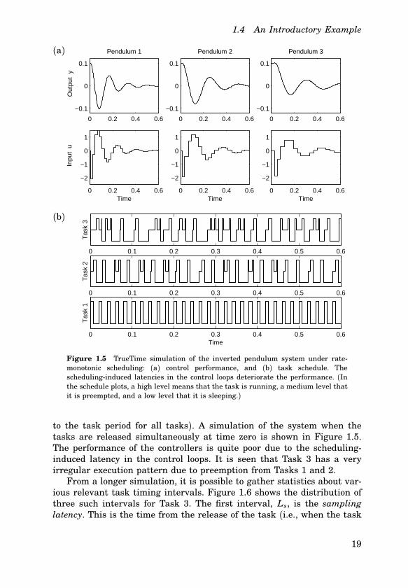
Figure 1.5 TrueTime simulation of the inverted pendulum system under rate­monotonic scheduling: (a) control performance, and (b) task schedule. Thescheduling­induced latencies in the control loops deteriorate the performance. (Inthe schedule plots, a high level means that the task is running, a medium level thatit is preempted, and a low level that it is sleeping.)

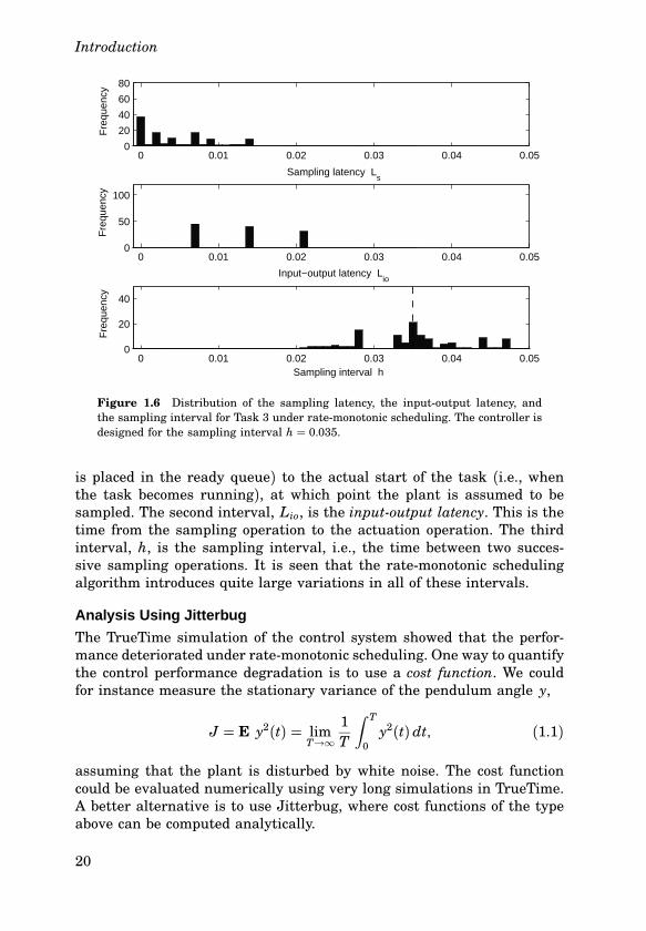
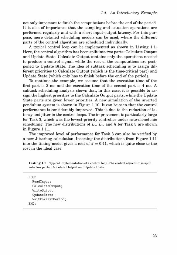
to the task period for all tasks). A simulation of the system when thetasks are released simultaneously at time zero is shown in Figure 1.5.The performance of the controllers is quite poor due to the scheduling­induced latency in the control loops. It is seen that Task 3 has a veryirregular execution pattern due to preemption from Tasks 1 and 2.From a longer simulation, it is possible to gather statistics about var­

ious relevant task timing intervals. Figure 1.6 shows the distribution ofthree such intervals for Task 3. The first interval, Ls, is the samplinglatency. This is the time from the release of the task (i.e., when the task

19

Introduction

0 0.01 0.02 0.03 0.04 0.050

20

40

60

80

Sampling latency Ls

Fre

quen

cy

0 0.01 0.02 0.03 0.04 0.050

50

100

Input−output latency Lio

Fre

quen

cy

0 0.01 0.02 0.03 0.04 0.050

20

40

Sampling interval h

Fre

quen

cy

Figure 1.6 Distribution of the sampling latency, the input­output latency, andthe sampling interval for Task 3 under rate­monotonic scheduling. The controller isdesigned for the sampling interval h = 0.035.

is placed in the ready queue) to the actual start of the task (i.e., whenthe task becomes running), at which point the plant is assumed to besampled. The second interval, Lio, is the input­output latency. This is thetime from the sampling operation to the actuation operation. The thirdinterval, h, is the sampling interval, i.e., the time between two succes­sive sampling operations. It is seen that the rate­monotonic schedulingalgorithm introduces quite large variations in all of these intervals.

Analysis Using Jitterbug

The TrueTime simulation of the control system showed that the perfor­mance deteriorated under rate­monotonic scheduling. One way to quantifythe control performance degradation is to use a cost function. We couldfor instance measure the stationary variance of the pendulum angle y,

J = E y2(t) = limT→∞

1T

∫ T

0y2(t) dt, (1.1)

assuming that the plant is disturbed by white noise. The cost functioncould be evaluated numerically using very long simulations in TrueTime.A better alternative is to use Jitterbug, where cost functions of the typeabove can be computed analytically.

20

1.4 An Introductory Example

H1(z)

H1(z)

H2(z)

H2(z)

G(s)yu

1

2

3

Ls

Lio

(a) (b)

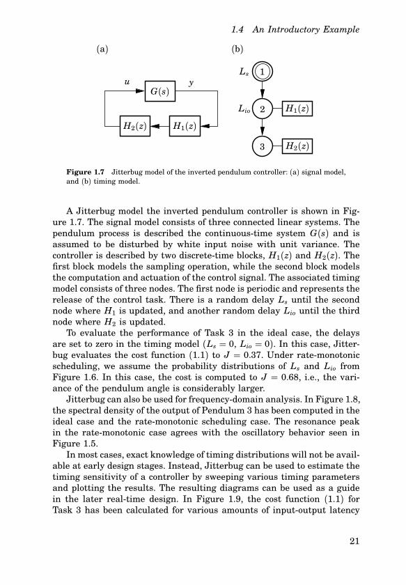
Figure 1.7 Jitterbug model of the inverted pendulum controller: (a) signal model,and (b) timing model.

A Jitterbug model the inverted pendulum controller is shown in Fig­ure 1.7. The signal model consists of three connected linear systems. Thependulum process is described the continuous­time system G(s) and isassumed to be disturbed by white input noise with unit variance. Thecontroller is described by two discrete­time blocks, H1(z) and H2(z). Thefirst block models the sampling operation, while the second block modelsthe computation and actuation of the control signal. The associated timingmodel consists of three nodes. The first node is periodic and represents therelease of the control task. There is a random delay Ls until the secondnode where H1 is updated, and another random delay Lio until the thirdnode where H2 is updated.To evaluate the performance of Task 3 in the ideal case, the delays

are set to zero in the timing model (Ls = 0, Lio = 0). In this case, Jitter­bug evaluates the cost function (1.1) to J = 0.37. Under rate­monotonicscheduling, we assume the probability distributions of Ls and Lio fromFigure 1.6. In this case, the cost is computed to J = 0.68, i.e., the vari­ance of the pendulum angle is considerably larger.Jitterbug can also be used for frequency­domain analysis. In Figure 1.8,

the spectral density of the output of Pendulum 3 has been computed in theideal case and the rate­monotonic scheduling case. The resonance peakin the rate­monotonic case agrees with the oscillatory behavior seen inFigure 1.5.In most cases, exact knowledge of timing distributions will not be avail­

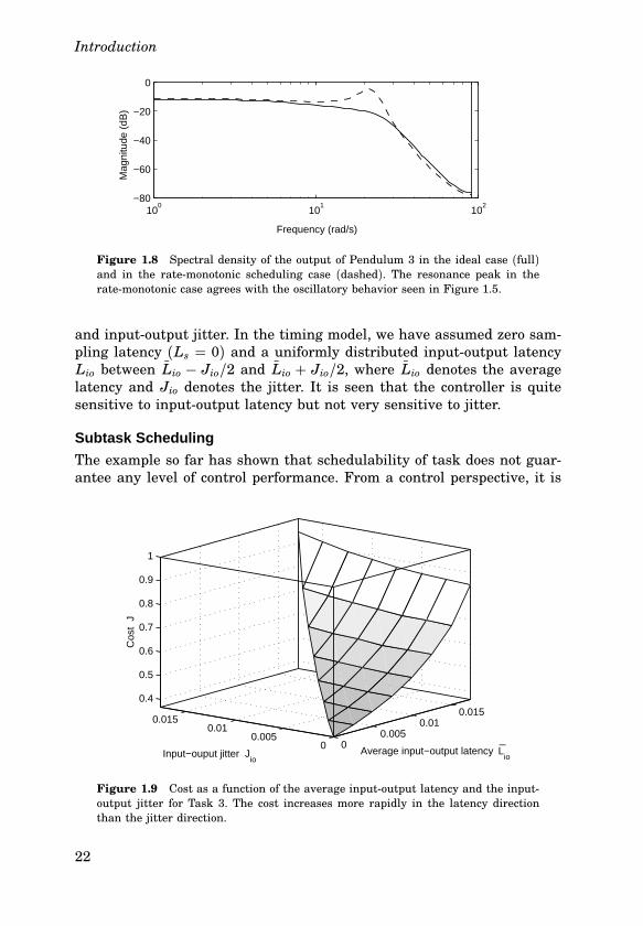
able at early design stages. Instead, Jitterbug can be used to estimate thetiming sensitivity of a controller by sweeping various timing parametersand plotting the results. The resulting diagrams can be used as a guidein the later real­time design. In Figure 1.9, the cost function (1.1) forTask 3 has been calculated for various amounts of input­output latency

21

Introduction

Frequency (rad/s)

Mag

nitu

de (

dB)

100

101

102

−80

−60

−40

−20

0

Figure 1.8 Spectral density of the output of Pendulum 3 in the ideal case (full)and in the rate­monotonic scheduling case (dashed). The resonance peak in therate­monotonic case agrees with the oscillatory behavior seen in Figure 1.5.

and input­output jitter. In the timing model, we have assumed zero sam­pling latency (Ls = 0) and a uniformly distributed input­output latencyLio between Lio − Jio/2 and Lio + Jio/2, where Lio denotes the averagelatency and Jio denotes the jitter. It is seen that the controller is quitesensitive to input­output latency but not very sensitive to jitter.

Subtask Scheduling

The example so far has shown that schedulability of task does not guar­antee any level of control performance. From a control perspective, it is

00.005

0.010.015

00.005

0.010.015

0.4

0.5

0.6

0.7

0.8

0.9

1

Average input−output latency LioInput−ouput jitter J

io

Cos

t J

_

Figure 1.9 Cost as a function of the average input­output latency and the input­output jitter for Task 3. The cost increases more rapidly in the latency directionthan the jitter direction.

22

1.4 An Introductory Example

not only important to finish the computations before the end of the period.It is also of importance that the sampling and actuation operations areperformed regularly and with a short input­output latency. For this pur­pose, more detailed scheduling models can be used, where the differentparts of the control algorithm are scheduled individually.A typical control loop can be implemented as shown in Listing 1.1.

Here, the control algorithm has been split into two parts: Calculate Outputand Update State. Calculate Output contains only the operations neededto produce a control signal, while the rest of the computations are post­poned to Update State. The idea of subtask scheduling is to assign dif­ferent priorities to Calculate Output (which is the time­critical part) andUpdate State (which only has to finish before the end of the period).To continue the example, we assume that the execution time of the

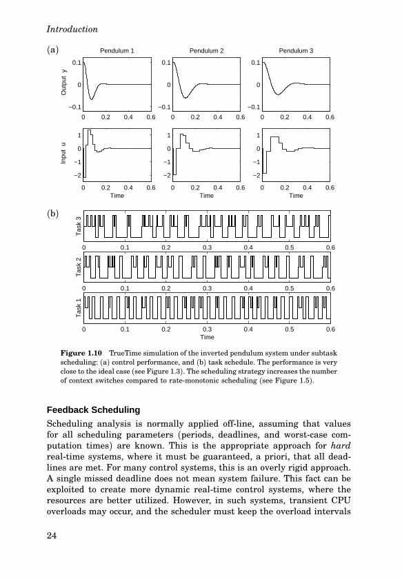
first part is 3 ms and the execution time of the second part is 4 ms. Asubtask scheduling analysis shows that, in this case, it is possible to as­sign the highest priorities to the Calculate Output parts, while the UpdateState parts are given lower priorities. A new simulation of the invertedpendulum system is shown in Figure 1.10. It can be seen that the controlperformance is considerably improved. This is due to the reduction of la­tency and jitter in the control loops. The improvement is particularly largefor Task 3, which was the lowest­priority controller under rate­monotonicscheduling. The new distributions of Ls, Lio and h for Task 3 are shownin Figure 1.11.The improved level of performance for Task 3 can also be verified by

a new Jitterbug calculation. Inserting the distributions from Figure 1.11into the timing model gives a cost of J = 0.41, which is quite close to thecost in the ideal case.

Listing 1.1 Typical implementation of a control loop. The control algorithm is splitinto two parts: Calculate Output and Update State.

LOOP

ReadInput;

CalculateOutput;

WriteOutput;

UpdateState;

WaitForNextPeriod;

END;

23

Introduction

(a)

0 0.2 0.4 0.6

−0.1

0

0.1O

utpu

t y

Pendulum 1

0 0.2 0.4 0.6

−0.1

0

0.1

Pendulum 2

0 0.2 0.4 0.6

−0.1

0

0.1

Pendulum 3

0 0.2 0.4 0.6

−2

−1

0

1

Time

Inpu

t u

0 0.2 0.4 0.6

−2

−1

0

1

Time0 0.2 0.4 0.6

−2

−1

0

1

Time

(b)

0 0.1 0.2 0.3 0.4 0.5 0.6

Tas

k 1

Time

0 0.1 0.2 0.3 0.4 0.5 0.6

Tas

k 2

0 0.1 0.2 0.3 0.4 0.5 0.6

Tas

k 3

Figure 1.10 TrueTime simulation of the inverted pendulum system under subtaskscheduling: (a) control performance, and (b) task schedule. The performance is veryclose to the ideal case (see Figure 1.3). The scheduling strategy increases the numberof context switches compared to rate­monotonic scheduling (see Figure 1.5).

Feedback Scheduling

Scheduling analysis is normally applied off­line, assuming that valuesfor all scheduling parameters (periods, deadlines, and worst­case com­putation times) are known. This is the appropriate approach for hardreal­time systems, where it must be guaranteed, a priori, that all dead­lines are met. For many control systems, this is an overly rigid approach.A single missed deadline does not mean system failure. This fact can beexploited to create more dynamic real­time control systems, where theresources are better utilized. However, in such systems, transient CPUoverloads may occur, and the scheduler must keep the overload intervals

24

1.4 An Introductory Example

0 0.01 0.02 0.03 0.04 0.050

20

40

60

80

Sampling latency Ls

Fre

quen

cy

0 0.01 0.02 0.03 0.04 0.050

50

100

Input−output latency Lio

Fre

quen

cy

0 0.01 0.02 0.03 0.04 0.050

20

40

Sampling interval h

Fre

quen

cy

Figure 1.11 Distribution of the sampling latency, the input­output latency, andthe sampling interval for Task 3 under subtask scheduling. Compared with the rate­monotonic scheduling case (Figure 1.6), the latencies are shorter and the samplinginterval is more closely centered around the nominal interval h = 0.035.

as short as possible.To continue the example, suppose that the execution time of the con­

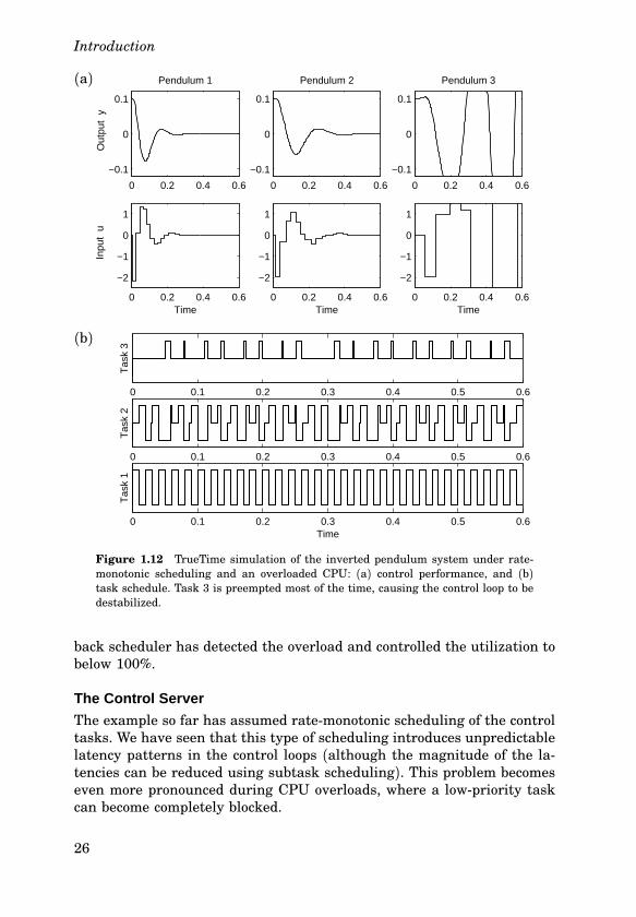
trol algorithm has been underestimated. The designer believes that theexecution time is 7 ms, while the true execution time is 10 ms. Using thesame sampling periods as before, the CPU utilization is now

U =∑ C

hi= 1.13,

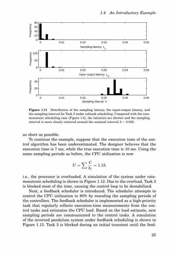
i.e., the processor is overloaded. A simulation of the system under rate­monotonic scheduling is shown in Figure 1.12. Due to the overload, Task 3is blocked most of the time, causing the control loop to be destabilized.Next, a feedback scheduler is introduced. The scheduler attempts to

control the CPU utilization to 80% by rescaling the sampling periods ofthe controllers. The feedback scheduler is implemented as a high­prioritytask that regularly collects execution­time measurements from the con­trol tasks and estimates the CPU load. Based on the load estimate, newsampling periods are communicated to the control tasks. A simulationof the inverted pendulum system under feedback scheduling is shown inFigure 1.13. Task 3 is blocked during an initial transient until the feed­

25

Introduction

(a)

0 0.2 0.4 0.6

−0.1

0

0.1O

utpu

t y

Pendulum 1

0 0.2 0.4 0.6

−0.1

0

0.1

Pendulum 2

0 0.2 0.4 0.6

−0.1

0

0.1

Pendulum 3

0 0.2 0.4 0.6

−2

−1

0

1

Time

Inpu

t u

0 0.2 0.4 0.6

−2

−1

0

1

Time0 0.2 0.4 0.6

−2

−1

0

1

Time

(b)

0 0.1 0.2 0.3 0.4 0.5 0.6

Tas

k 1

Time

0 0.1 0.2 0.3 0.4 0.5 0.6

Tas

k 2

0 0.1 0.2 0.3 0.4 0.5 0.6

Tas

k 3

Figure 1.12 TrueTime simulation of the inverted pendulum system under rate­monotonic scheduling and an overloaded CPU: (a) control performance, and (b)task schedule. Task 3 is preempted most of the time, causing the control loop to bedestabilized.

back scheduler has detected the overload and controlled the utilization tobelow 100%.

The Control Server

The example so far has assumed rate­monotonic scheduling of the controltasks. We have seen that this type of scheduling introduces unpredictablelatency patterns in the control loops (although the magnitude of the la­tencies can be reduced using subtask scheduling). This problem becomeseven more pronounced during CPU overloads, where a low­priority taskcan become completely blocked.

26

1.4 An Introductory Example

(a)

0 0.2 0.4 0.6

−0.1

0

0.1O

utpu

t y

Pendulum 1

0 0.2 0.4 0.6

−0.1

0

0.1

Pendulum 2

0 0.2 0.4 0.6

−0.1

0

0.1

Pendulum 3

0 0.2 0.4 0.6

−2

−1

0

1

Time

Inpu

t u

0 0.2 0.4 0.6

−2

−1

0

1

Time0 0.2 0.4 0.6

−2

−1

0

1

Time

(b)

0 0.1 0.2 0.3 0.4 0.5 0.6

Tas

k 1

Time

0 0.1 0.2 0.3 0.4 0.5 0.6

Tas

k 2

0 0.1 0.2 0.3 0.4 0.5 0.6

Tas

k 3

0 0.1 0.2 0.3 0.4 0.5 0.6

FB

S

Figure 1.13 TrueTime simulation of the inverted pendulum system under feed­back scheduling: (a) control performance, and (b) task schedule. The feedback sched­uler (FBS) regularly adjusts the sampling periods of the controllers, resolving theinitial overload situation.

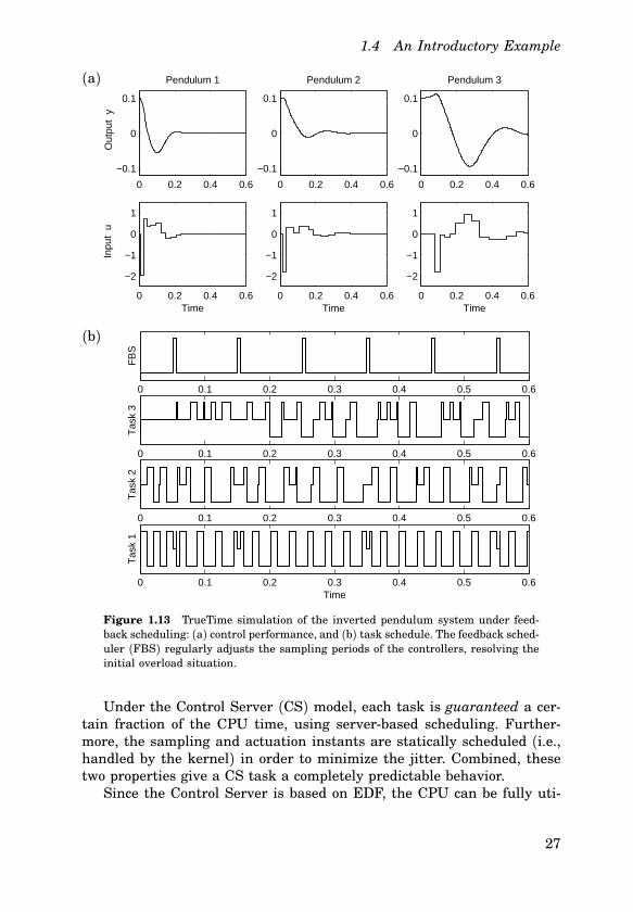
Under the Control Server (CS) model, each task is guaranteed a cer­tain fraction of the CPU time, using server­based scheduling. Further­more, the sampling and actuation instants are statically scheduled (i.e.,handled by the kernel) in order to minimize the jitter. Combined, thesetwo properties give a CS task a completely predictable behavior.Since the Control Server is based on EDF, the CPU can be fully uti­

27

Introduction

(a)

0 0.2 0.4 0.6

−0.1

0

0.1O

utpu

t y

Pendulum 1

0 0.2 0.4 0.6

−0.1

0

0.1

Pendulum 2

0 0.2 0.4 0.6

−0.1

0

0.1

Pendulum 3

0 0.2 0.4 0.6

−2

−1

0

1

Time

Inpu

t u

0 0.2 0.4 0.6

−2

−1

0

1

Time0 0.2 0.4 0.6

−2

−1

0

1

Time

(b)

0 0.1 0.2 0.3 0.4 0.5 0.6

Tas

k 1

Time

0 0.1 0.2 0.3 0.4 0.5 0.6

Tas

k 2

0 0.1 0.2 0.3 0.4 0.5 0.6

Tas

k 3

0 0.1 0.2 0.3 0.4 0.5 0.6

Ker

nel

Figure 1.14 TrueTime simulation of the inverted pendulum system under theControl Server model: (a) control performance, and (b) task schedule. The perfor­mance is very close to the ideal case (see Figure 1.3). The kernel handles the I/Ooperations of all the control tasks.

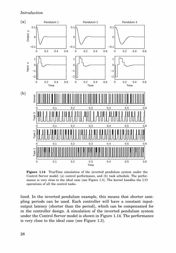
lized. In the inverted pendulum example, this means that shorter sam­pling periods can be used. Each controller will have a constant input­output latency (shorter than the period), which can be compensated forin the controller design. A simulation of the inverted pendulum systemunder the Control Server model is shown in Figure 1.14. The performanceis very close to the ideal case (see Figure 1.3).

28

1.5 Outline and Publications

1.5 Outline and Publications

The outline of the thesis is given below, together with references to relatedpublications.

Chapter 2: Background

An introduction to real­time scheduling theory is given, followed by anoverview of control loop timing. A brief survey of existing control andscheduling codesign approaches is given.

Publications

Årzén, K.­E., B. Bernhardsson, J. Eker, A. Cervin, K. Nilsson, P. Persson,and L. Sha (1999): “Integrated control and scheduling.” TechnicalReport ISRN LUTFD2/TFRT­­7586­­SE. Department of AutomaticControl, Lund Institute of Technology, Sweden.

Årzén, K.­E., A. Cervin, J. Eker, and L. Sha (2000): “An introduction tocontrol and scheduling co­design.” In Proceedings of the 39th IEEEConference on Decision and Control. Sydney, Australia.

Cervin, A. (2000): “Towards the integration of control and real­timescheduling design.” Licentiate Thesis ISRN LUTFD2/TFRT­­3226­­SE. Department of Automatic Control, Lund Institute of Technology,Sweden.

The Bluetooth jitter compensation example appears in

Eker, J., A. Cervin, and A. Hörjel (2001): “Distributed wireless controlusing Bluetooth.” In Proceedings of the IFAC Conference on NewTechnologies for Computer Control. Hong Kong, P.R. China.

Chapter 3: Subtask Scheduling

This chapter considers scheduling of simple controllers where the controlalgorithm has been split into two parts: Calculate Output and UpdateState. The goal is to reduce the input­output latencies in the control loops.Subtask deadline assignment under fixed­priority and earliest­deadlinefirst scheduling is treated. The control performance improvements areverified in an inverted pendulum example.

Publications

Cervin, A. (1999): “Improved scheduling of control tasks.” In Proceedingsof the 11th Euromicro Conference on Real­Time Systems. York, UK.

29

Introduction

Chapter 4: Feedback Scheduling

A scheduling architecture is proposed, where the CPU load is controlledby adjusting the sampling intervals of a set of controllers. The goal is tomaintain high utilization and good control performance in spite of largevariations in execution time. Feedforward from mode changes is used tofurther improve the regulation. A heuristic approach is discussed first,where simple rescaling of the nominal sampling periods to reach the uti­lization setpoint is used. The approach is exemplified on a set of hybridcontrollers. It is later shown that simple period rescaling is in fact op­timal for controllers with certain cost functions. Overloaded open­loopEDF scheduling is also discussed, and it is shown that overloaded EDF isequivalent to linear period rescaling.

Publications

Cervin, A. and J. Eker (2000): “Feedback scheduling of control tasks.”In Proceedings of the 39th IEEE Conference on Decision and Control.Sydney, Australia.

Persson, P., A. Cervin, and J. Eker (2000): “Execution­time properties ofa hybrid controller.” Technical Report ISRN LUTFD2/TFRT­­7591­­SE. Department of Automatic Control, Lund Institute of Technology,Sweden.

Cervin, A., J. Eker, B. Bernhardsson, and K.­E. Årzén (2002): “Feedback­feedforward scheduling of control tasks.” Real­Time Systems, 23:1/2.

A preliminary study of feedback scheduling of model predictive controllersis presented in

Henriksson, D., A. Cervin, J. Åkesson, and K.­E. Årzén (2002): “Feedbackscheduling of model predictive controllers.” In Proceedings of the8th IEEE Real­Time and Embedded Technology and ApplicationsSymposium. San Jose, CA.

Chapter 5: The Control Server

A new computational model for real­time control tasks is presented, withthe primary goal of simplifying the control and scheduling codesign prob­lem. The model combines time­triggered I/O and inter­task communica­tion with dynamic, reservation­based task scheduling. To facilitate shortinput­output latencies, a task may be divided into several segments. Jitteris reduced by allowing communication only at the beginning and at theend of a segment. A key property of the model is that both schedulabil­ity and control performance of a control task will depend on the reservedutilization factor only. This enables controllers to be treated as scalable

30

1.5 Outline and Publications

real­time components. The model has been implemented in a public do­main real­time kernel and validated in control experiments.

Publications

Cervin, A. and J. Eker (2003): “The Control Server: A computationalmodel for real­time control tasks.” In Proceedings of the 15th Euromi­cro Conference on Real­Time Systems. Porto, Portugal. (To appear inJune 2003.)

Chapter 6: Analysis Using Jitterbug

The MATLAB­based toolbox Jitterbug is presented. The tool allows theuser to compute a quadratic performance index for a control loop undervarious timing conditions. The control system is built from a number ofcontinuous­ and discrete­time linear systems, and the execution of thecontroller is described by a stochastic timing model. The toolbox is alsocapable of computing the spectral densities of the signals in the system.Using the tool, it is easy to investigate the impact of delays, jitter, lostsamples, aperiodic execution, etc., on the control performance. A numberof examples are given.

Publications

Lincoln, B. and A. Cervin (2002): “Jitterbug: A tool for analysis of real­time control performance.” In Proceedings of the 41st IEEE Conferenceon Decision and Control. Sydney, Australia.

Cervin, A. and B. Lincoln (2003): “Jitterbug 1.1—Reference manual.”Technical Report ISRN LUTFD2/TFRT­­7604­­SE. Department ofAutomatic Control, Lund Institute of Technology, Sweden.

(There are also two publications that describe both Jitterbug and True­Time, see below.)

Chapter 7: Simulation Using TrueTime

The MATLAB/Simulink­based simulator TrueTime is presented. The sim­ulator allows detailed co­simulation of continuous plant dynamics, real­time scheduling, control task execution, and message transmission indistributed real­time control systems. The TrueTime Kernel block is de­scribed in detail, and a number of examples are given.

Publications

Henriksson, D., A. Cervin, and K.­E. Årzén (2002): “TrueTime: Simulationof control loops under shared computer resources.” In Proceedings

31

Introduction

of the 15th IFAC World Congress on Automatic Control. Barcelona,Spain.

Henriksson, D. and A. Cervin (2003): “TrueTime 1.1—Reference manual.”Technical Report ISRN LUTFD2/TFRT­­7605­­SE. Department ofAutomatic Control, Lund Institute of Technology, Sweden.

Both Jitterbug and TrueTime are described in

Cervin, A., D. Henriksson, B. Lincoln, and K.­E. Årzén (2002): “Jitter­bug and TrueTime: Analysis tools for real­time control systems.” InProceedings of the 2nd Workshop on Real­Time Tools. Copenhagen,Denmark.

Cervin, A., D. Henriksson, B. Lincoln, J. Eker, and K.­E. Årzén (2003):“How does control timing affect performance?” IEEE Control SystemsMagazine. (To appear in June 2003.)

An old version of the simulator is described in

Eker, J. and A. Cervin (1999): “A Matlab toolbox for real­time and controlsystems co­design.” In Proceedings of the 6th International Conferenceon Real­Time Computing Systems and Applications. Hong Kong, P.R.China.

Cervin, A. (2000): “The real­time control systems simulator—Referencemanual.” Technical Report ISRN LUTFD2/TFRT­­7592­­SE. Depart­ment of Automatic Control, Lund Institute of Technology, Sweden.

Chapter 8: Conclusion

The contents of the thesis are summarized and suggestions for futurework are given.

32

2

Background

2.1 Introduction

In textbooks on real­time systems, e.g., [Burns and Wellings, 2001; Liu,2000; Buttazzo, 1997; Krishna and Shin, 1997], control systems are usedas the prime example of hard real­time systems. In a hard real­time sys­tem, the computer must respond to events within specified deadlines—otherwise, the system will fail. In the case of a control system, the com­puter must respond to incoming measurement signals, producing newcontrol signals fast enough to keep the plant within its operational limits.The controller is often just one component among many in an embed­

ded computer system. There may be several more controllers executingon the same unit, together with communication tasks, operator interfaces,tasks for data logging, etc. The concurrent activities are typically imple­mented on a microprocessor using a sequential programming languagesuch as C together with a real­time operating system, or using a moremodern language such as Ada or Java that has direct support for concur­rent programming.In an embedded system, the processor (CPU) time is a shared resource

for which the various tasks compete. To guarantee, a priori, that all taskswill meet their deadlines, static (off­line) schedulability analysis mustbe performed. The analysis assumes a certain task model and that therelevant task attributes are known. The traditional view in the hard real­time scheduling community is that a digital controller can be modeled asa task that has

• a fixed period,

• a hard deadline equal to the period, and

• a known worst­case execution time (WCET).

33

Background

Process

A­DControlAlgorithmD­A

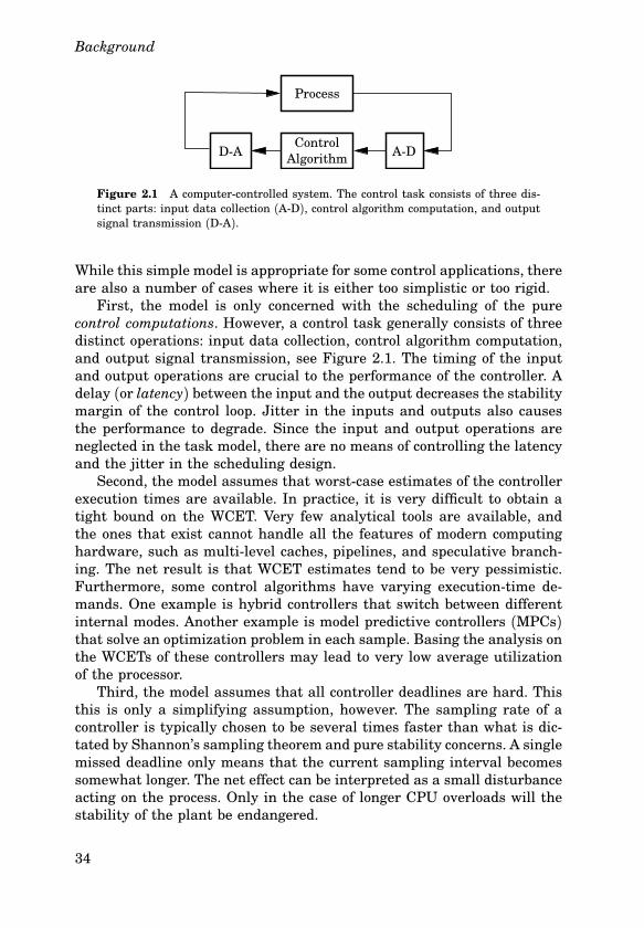
Figure 2.1 A computer­controlled system. The control task consists of three dis­tinct parts: input data collection (A­D), control algorithm computation, and outputsignal transmission (D­A).

While this simple model is appropriate for some control applications, thereare also a number of cases where it is either too simplistic or too rigid.First, the model is only concerned with the scheduling of the pure

control computations. However, a control task generally consists of threedistinct operations: input data collection, control algorithm computation,and output signal transmission, see Figure 2.1. The timing of the inputand output operations are crucial to the performance of the controller. Adelay (or latency) between the input and the output decreases the stabilitymargin of the control loop. Jitter in the inputs and outputs also causesthe performance to degrade. Since the input and output operations areneglected in the task model, there are no means of controlling the latencyand the jitter in the scheduling design.Second, the model assumes that worst­case estimates of the controller

execution times are available. In practice, it is very difficult to obtain atight bound on the WCET. Very few analytical tools are available, andthe ones that exist cannot handle all the features of modern computinghardware, such as multi­level caches, pipelines, and speculative branch­ing. The net result is that WCET estimates tend to be very pessimistic.Furthermore, some control algorithms have varying execution­time de­mands. One example is hybrid controllers that switch between differentinternal modes. Another example is model predictive controllers (MPCs)that solve an optimization problem in each sample. Basing the analysis onthe WCETs of these controllers may lead to very low average utilizationof the processor.Third, the model assumes that all controller deadlines are hard. This

this is only a simplifying assumption, however. The sampling rate of acontroller is typically chosen to be several times faster than what is dic­tated by Shannon’s sampling theorem and pure stability concerns. A singlemissed deadline only means that the current sampling interval becomessomewhat longer. The net effect can be interpreted as a small disturbanceacting on the process. Only in the case of longer CPU overloads will thestability of the plant be endangered.

34

2.2 Real­Time Scheduling Theory

In the following chapters of the thesis, modifications to the simpletask model that remedy some of the problems above will be given. Moredetailed task models allow better control of latency and jitter in the controlloops. Relaxing the requirements on known WCETs and hard deadlinesallows the computing resources to be used more efficiently. Accepting somedegree of non­determinism in real­time control systems also permits theuse of COTS hardware and software. This can lead to lower developmentcosts for embedded systems.The rest of this chapter contains background material on real­time

scheduling theory, control loop timing, and related work in the area ofcontrol and real­time scheduling codesign.

2.2 Real-Time Scheduling Theory

Real­time scheduling theory is used to predict whether the tasks in areal­time system will meet their individual timing requirements. Given atask model and a scheduling algorithm, off­line analysis is performed tocheck, for instance, whether all deadlines will be met during runtime.Two main design approaches exist: static scheduling and dynamic

scheduling. Static scheduling is an off­line approach that uses optimization­based algorithms to generate a cyclic executive. An execution table statesthe order in which the different tasks should execute and for how long theyshould execute. An advantage of the cyclic executive is that it is very sim­ple to implement. The approach also has many drawbacks [Locke, 1992].First, there is the difficulty of constructing the schedule itself. Second,it is hard to incorporate sporadic and aperiodic tasks. Third, tasks withlong execution times may have to be split in many small pieces, makingthe code error­prone and difficult to read. Fourth, very long tables maybe needed if the schedule incorporates tasks with period times that arerelative prime. Due to these drawbacks, we will mainly consider dynamicscheduling in the sequel.There exist a large number of dynamic scheduling policies. Here we

will focus on the fixed­priority (FP) and the earliest­deadline­first (EDF)scheduling policies, both introduced in the seminal paper [Liu and Lay­land, 1973]. In the scheduling analysis, a basic task model is assumed,where each task τ i is described by

• a period (or minimum inter­arrival time) Ti,• a relative deadline Di, and

• a worst­case execution time Ci.

35

Background

Furthermore, in the simplest case, it is assumed that the tasks are inde­pendent (i.e., they do not communicate or share other resources than theCPU), and that there is no kernel overhead.

Fixed-Priority Scheduling

Fixed­priority (FP) scheduling is the most common scheduling policy andis supported by most commercial real­time operating systems. Under FPscheduling, each task τ i is assigned a fixed priority Pi. If several tasksare ready to run at the same time, the task with the highest priority getsaccess to the CPU. If a task with higher priority than the running taskshould become ready, the running task is preempted by the other task.

Priority Assignment. Fixed­priority scheduling design consists of as­signing priorities to all tasks before runtime. In [Liu and Layland, 1973]it was shown that the rate­monotonic (RM) priority assignment is opti­mal when Di = Ti for all tasks. Each task is assigned a priority based onits period: the shorter the period, the higher the priority. The scheme isoptimal in the sense that, if the task set is not schedulable under the rate­monotonic priority assignment, it will not be schedulable under any otherfixed­priority assignment. By rate­monotonic scheduling, we mean fixed­priority scheduling where the tasks have been assigned rate­monotonicpriorities.In many cases, it is desirable to specify deadlines that are shorter than

the period. In the case where Di ≤ Ti for all tasks, the deadline­monotonic(DM) priority assignment scheme is optimal (in the same sense as above)[Leung and Whitehead, 1982]. Each task is assigned a priority based onits relative deadline: the shorter the deadline, the higher the priority.Note that the RM priority assignment is merely a special case of the DMpriority assignment.

Schedulability Analysis. Given a task set with known attributes (pe­riods, deadlines, execution times, and priorities), a number of differenttests can be applied to check whether all tasks will meet their deadlines.Assuming the rate­monotonic priority assignment, a sufficient (but notnecessary) schedulability test is obtained by considering the utilization ofthe task set [Liu and Layland, 1973]. Assuming a set of n tasks, all taskswill meet their deadlines if

U =n

∑

i=1

Ci

Ti≤ n(21/n − 1). (2.1)

As the number of tasks becomes large, the utilization bound approachesln 2 � 0.693.

36

2.2 Real­Time Scheduling Theory

An exact schedulability test under FP scheduling is performed by com­puting the worst­case response time Ri of each task [Joseph and Pandya,1986]. The response time of a task is defined as the time from its releaseto its completion. The maximum response time of a task occurs when allother tasks are released simultaneously. The worst­case response time ofa task τ i is given by the recursive equation

Ri = Ci +∑

j∈hp(i)

⌈

Ri

Tj

⌉

Cj (2.2)

where hp(i) is the set of tasks with higher priority than τ i and dxf denotesthe ceiling function. The task set is schedulable if and only if Ri ≤ Di forall tasks.

Extensions. Many extensions to the theory of FP scheduling exist, e.g.,[Klein et al., 1993]. The analysis has been extended to handle for in­stance common resources, release jitter, tick scheduling, nonzero context­switching times, and clock interrupts.The analysis behind the schedulability conditions is based on the no­

tion of the critical instant. This is the situation when all tasks are releasedsimultaneously. If the task set is schedulable for this worst case, it will beschedulable also for all other cases. In many cases, this assumption is un­necessarily restrictive. Tasks may have precedence constraints that makeit impossible for them to arrive at the same time. For independent tasks itis sometimes possible to introduce release offsets, to avoid the simultane­ous releases. If simultaneous releases can be avoided, the schedulabilityof the task set may increase [Audsley et al., 1993]. Formulas for exactresponse­time calculations for tasks with static release offsets is given in[Redell and Törngren, 2002]. Schedulability analysis for tasks with dy­namic offsets is discussed in [Gutierrez and Harbour, 1998]. A number ofalternative scheduling models based on serialization of task executions indifferent ways have been suggested. These include the multi­frame model[Baruah et al., 1999b] and the serially executed subtask model [Harbouret al., 1994].Recently, formulas for the best­case response time of tasks under fixed­

priority scheduling have been derived [Redell and Sanfridson, 2002]. Know­ing both the worst­case and the best­case response time of a task givesa measure of the response­time jitter. In its simplest form, the best­caseresponse time Rbi of task τ i is given by the recursive equation

Rbi = Cbi +∑

j∈hp(i)

⌈

Rbi − TjTj

⌉

Cbj (2.3)

where Cbi denotes the best­case execution time of task τ i.

37

Background

Earliest-Deadline-First Scheduling

Under EDF scheduling, the task with the shortest time to its deadlineis chosen for execution. The absolute deadline of a task can hence beinterpreted as a dynamic priority. Because of its more dynamic nature,EDF can schedule a larger set of task sets than the FP scheduling policycan. Despite its theoretical advantages, EDF has so far mainly been usedin experimental real­time operating systems. A reason for this may be thatEDF also has a number of potential drawbacks compared to FP scheduling[Burns and Wellings, 2001]:

• The implementation of EDF is slightly more complex; the dynamicpriority incurs a larger runtime overhead and requires more storage.

• It may be difficult to assign artificial deadlines to tasks that haveno explicit deadlines.

• During overloads, all tasks tend to miss their deadlines (this isknown as the domino effect).

The arguments above should not be taken too seriously. It can be arguedthat it is more difficult to assign meaningful priorities than deadlines in areal­time system. Furthermore, control tasks running under EDF schedul­ing actually tend to behave better in overload situations than under FPscheduling (see Chapter 4).

Schedulability Analysis. In the case where Di = Ti for all tasks,the schedulability of a task set under EDF is exactly determined by theprocessor utilization [Liu and Layland, 1973]. All tasks will meet theirdeadlines if and only if

U =n

∑

i=1

Ci

Ti≤ 1. (2.4)

Note that this test is much simpler than the exact schedulability test un­der FP scheduling (which requires that the response times are computed).Also note that the processor can be fully utilized under EDF.For the case Di ≤ Ti, the analysis becomes more difficult. A very

general schedulability test under EDF involves computing the loadingfactor of the tasks (see [Stankovic et al., 1998]). The analysis is performedas follows. Given an arbitrary set of tasks, let each job (task instance) jkbe described by a computation time Ck, a release time rk, and an absolutedeadline dk. Define the processor demand of the task set on a time interval[t1, t2] as

h[t1, t2] =∑

rk≥t1 ∧ dk≤t2

Ck. (2.5)

38

2.2 Real­Time Scheduling Theory

Next, define the loading factor u of the tasks as

u = max0≤t1<t2

h[t1, t2]t2 − t1

, (2.6)

where the maximization is performed over all possible time intervals. Thetask set is schedulable under EDF if and only if u ≤ 1.

Response­Time Analysis. Worst­case response­time analysis underEDF scheduling is more difficult than under FP scheduling. The mainproblem is that there is no well­defined critical instance at which the taskwill experience its maximum interference. Nevertheless, formulas havebeen derived for response­time calculations under EDF, see [Stankovicet al., 1998].

Server-Based Scheduling

Many types of tasks do not fit the simple periodic task model. These in­clude aperiodic and soft real­time tasks. To retain the guarantees of thehard real­time tasks, these types of tasks can be incorporated in the real­time system using servers. The main idea of the server­based schedulingis to have a special task, the server, for scheduling the pending aperiodicworkload (emanating from one or several aperiodic tasks). The server hasa budget that is used to schedule and execute the pending jobs. The ape­riodic tasks may execute until they finish or until the budget has been ex­hausted. Several servers have been proposed. The priority­exchange serverand the deferrable server were proposed in [Lehoczky et al., 1987]. Thesporadic server was introduced in [Sprunt et al., 1989]. The main differ­ence between the servers concerns the way the budget is replenished andthe maximum capacity of the server.The above servers have been developed for the fixed­priority case. Sim­

ilar techniques also exist for the dynamic­priority case (i.e., EDF), see,e.g., [Spuri and Buttazzo, 1996]. An EDF­based server with especially in­teresting properties is the constant bandwidth server (CBS) [Abeni andButtazzo, 1998]. Since the server will be used in Chapter 5, it is describedin detail below.

The Constant Bandwidth Server. A CBS creates the abstraction ofa virtual CPU with a given capacity (or bandwidth) Us. Tasks executingwithin the CBS cannot consume more than the reserved capacity. Hence,from the outside, the CBS will appear as an ordinary EDF task witha maximum utilization of Us. The time granularity of the virtual CPUabstraction is determined by the server period Ts.Associated with the server are two dynamic attributes: the server bud­

get cs and the server deadline ds. Jobs that arrive to the server are placed

39

Background

2

00 2 4 6 8 10 12 14

0 2 4 6 8 10 12 14

Jobs

CBSbudget

j1 j2 j3

r1 r2 r3d1 d2, d3d′1 d′

3

t

t

Figure 2.2 Example of a constant bandwidth server (CBS) with the band­width Us = 0.5 and the period Ts = 4 serving aperiodically arriving jobs. Theup arrows indicate job arrivals, and the down arrows indicate deadlines.

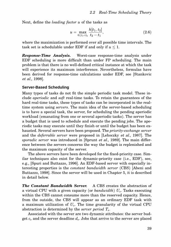
in a queue and are served on first­come, first­served basis. The first jobin the queue is always eligible for execution (as an ordinary EDF task),using the current server deadline ds. The server is initialized with cs := 0and ds := 0. The rules for updating the server are as follows:1. During the execution of a job, the budget cs is decreased at unit rate.

2. Whenever cs = 0, the budget is recharged to cs := UsTs and thedeadline is postponed one server period: ds := ds + Ts.

3. If a job arrives at a time r when the server queue is empty, and ifcs ≥ (ds − r)Us, then the budget is recharged to cs := UsTs and thedeadline is set to ds := r + Ts.

The above rules limit the server processor demand in any time in­terval [t1, t2] to Us(t2 − t1). The third rule is used to “reset” the serverafter a sufficiently long idle interval. Note that postponing the deadlinecorresponds to lowering the dynamic priority of the server.An example of CBS scheduling is given in Figure 2.2. The server is

assumed to have the bandwidth Us = 0.5 and the period Ts = 4. At t = 0,the server is empty and job j1 arrives. The budget is charged to UsTs = 2and the job is served with the deadline d1 = r1+Ts = 4 (rule 3). At t = 2,the budget is exhausted. The budget is recharged to UsTs = 2, and theremainder of j1 (one time unit) is served using the postponed deadlined′1 = d1+Ts = 8 (rule 2). At t = 7, job j2 arrives. Rule 3 is in effect, causingthe budget to be recharged and the deadline to be set to d2 = r2+Ts = 11.At t = 9, job j3 arrives. Rule 3 is not in effect, so the job is served withthe old server deadline d3 = d2 = 11. At t = 9.7, the budget is once againexhausted. The budget is recharged, and the remainder of the job (0.3units) is served using the postponed deadline d′

3 = d3 + Ts = 15.

40

2.3 Control Loop Timing

rk−1 rk rk+1

Lk−1io Lkio

hk−1 hk

Lk−1s Lks

t

III OO

Figure 2.3 Controller timing.

2.3 Control Loop Timing

A control loop consists of three main parts: input data collection, controlalgorithm computation, and output signal transmission. In the simplestcase the input and output operations consist of calls to an external I/Ointerface, e.g., A­D and D­A converters or a field­bus interface. In a morecomplex setting the input data may be received from other computationalblocks, such as noise filters, and the output signal may be sent to othercomputational blocks, e.g., other control loops in the case of set­point con­trol. The complexity of the control algorithm may range from a few linesof code implementing a PID (proportional­integral­derivative) controllerto the iterative solution of a quadratic optimization problem in the caseof model predictive control (MPC). In most cases the control is executedperiodically with a sampling interval that is determined by the dynamicsof the process that is controlled and the requirements on the closed­loopperformance. A typical rule­of­thumb [Åström and Wittenmark, 1997] isthat the sampling interval h should be selected such that

ω ch = 0.2–0.6, (2.7)

where ω c is the bandwidth of the closed­loop system. A real­time systemwhere the product ω ch is small for all control tasks will be less sensitiveto scheduling­induced latencies and jitter, but it will also consume moreCPU resources.

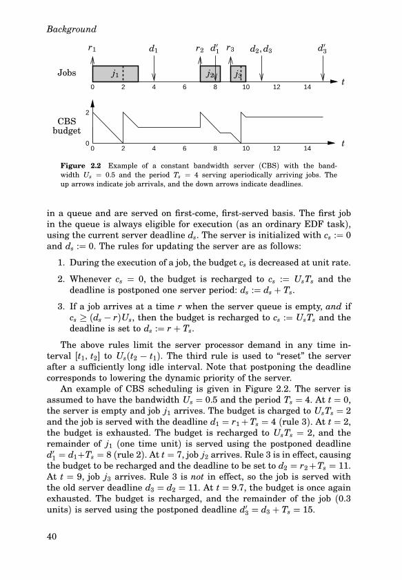
Timing Parameters

Ideally, the control algorithm should be executed with perfect periodicity,and there should be zero delay between the reading of the inputs and thewriting of the outputs. This will not be the case in a real implementation,where the execution and scheduling of tasks introduce latencies. The basictiming parameters of a control task are shown in Figure 2.3. It is assumedthat the control task is released (i.e., inserted into the ready queue of the

41

Background

real­time operating system) periodically at times given by rk = hk, whereh is the nominal sampling interval of the controller. Due to preemptionfrom other tasks in the system, the actual start of the task may be delayedfor some time Ls. This is called the sampling latency of the controller. Adynamic scheduling policy will introduce variations in this interval. Thesampling jitter is quantified by the difference between the maximum andminimum sampling latencies in all task instances,

Jsdef= Lmaxs − Lmins . (2.8)

Normally, it can be assumed that the minimum sampling latency of a taskis zero, in which case we have Js = Lmaxs . Jitter in the sampling latencywill of course also introduce jitter in the sampling interval h. From thefigure, it is seen that the actual sampling interval in period k is given by

hk = h− Lk−1s + Lks . (2.9)

The sampling interval jitter is quantified by

Jhdef= hmax − hmin. (2.10)

We can see that the sampling interval jitter is upper bounded by

Jh ≤ 2Js. (2.11)

After some computation time and possibly further preemption from othertasks, the controller will actuate the control signal. The delay from thesampling to the actuation is the input­output latency, denoted Lio. Vary­ing execution times or task scheduling will introduce variations in thisinterval. The input­output jitter is quantified by

Jiodef= Lmaxio − Lminio . (2.12)

The impact of input­output latency, input­output jitter, and sampling jitteron the control design and the scheduling design is discussed below.

Input-Output Latency

Control Design. It is well known that a constant input­output latencydecreases the phase margin of the control system, and that it introducesa fundamental limitation on the achievable closed­loop performance. Theresulting sampled­data system is time­invariant and of finite order, whichallows standard linear time­invariant (LTI) analysis to be used (see e.g.,

42

2.3 Control Loop Timing

[Åström andWittenmark, 1997]). For a given value of the latency, it is easyto predict the performance degradation due to the delay. Furthermore,it is straightforward to account for a constant latency in most controldesign methods. From this perspective, a constant input­output latencyis preferable over a varying latency.

Scheduling Design. The scheduling­induced input­output latency ofa single control task can be reduced by assigning it a higher priority (or,alternatively, under EDF scheduling, a shorter deadline). This approachwill of course not work for the whole task set.Another option is to use non­preemptive scheduling. This will guar­

antee that, once the task has started its execution, it will continue unin­terrupted until the end. The disadvantages of this approach are that thescheduling analysis for non­preemptive scheduling is quite complicated(e.g., [Klein et al., 1993; Stankovic et al., 1998]), and that the schedula­bility of other the tasks may be compromised.A standard way to achieve a short input­output latency in a control

task is to separate the algorithm calculations in two parts: Calculate Out­put and Update State. Calculate Output contains only the parts of the al­gorithm that make use of the current sample information. Update Statecontains the update of the controller states and precalculations for thenext period. Update State can therefore be executed after the output sig­nal transmission, hence, reducing the input­output latency. Further im­provements can be obtained by scheduling the two parts as subtasks. Thisis the topic of the next chapter of the thesis.

Input-Output Jitter

Control Design. A control system with a time­varying input­output la­tency is quite difficult to analyze, since the standard tools for LTI systemscannot be used. If the statistical properties of the latency are known, thentheory from jump linear systems can be used to evaluate the stability andperformance of the system (in the mean sense), see [Nilsson, 1998a]. Asimilar approach is taken in the Jitterbug toolbox (see Chapter 6), wherethe latency is described by a random variable that is assumed to be inde­pendent from sample to sample.Often, it is not possible to have exact knowledge of the input­output

latency distribution. A simple, sufficient stability test for systems whereonly the range of the latency is known is given in [Lincoln, 2002b]. As­suming zero sampling jitter, the test can guarantee stability for any input­output latencies in a given interval (whether they are time­varying, de­pendent, etc.).One approach to deal with jitter in the control design is to explicitly

43

Background

Actuatornode Process Sensor

node

Controllernode

Network

h

τ kscτ kca

u(t) y(t)

Figure 2.4 Distributed digital control system with network communication delaysτ sckand τ ca

k. From [Nilsson, 1998a].

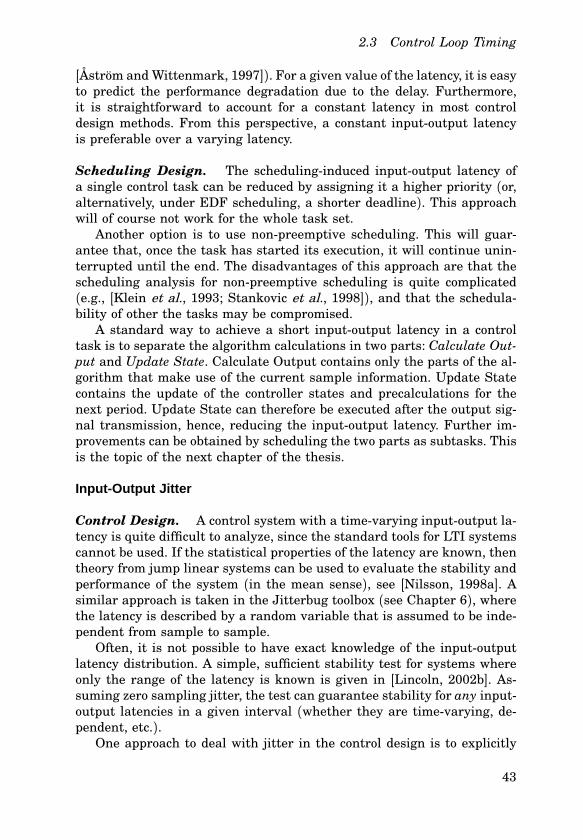
design the controller to be robust, i.e., the delay is treated as a paramet­ric uncertainty. Many robust design methods can be used, such as H∞,quantitative feedback theory (QFT) and µ­design.Another approach is to let the controller actively compensate for the

delay in each sample. An optimal, jitter­compensating controller was de­veloped in [Nilsson, 1998a]. The controller compensates for time­varyingdelays in a control loop, which is closed over a communication network.The setup is shown in Figure 2.4. The sensor node samples the processperiodically, sending the measurements over the network to the controllernode. The controller node is event­driven and computes a new control sig­nal as soon as a measurement arrives. The control signal is sent to theevent­driven actuator node, which outputs the signal to the process. TheLQ (linear­quadratic) state feedback control law has the form

u(k) = −L(τ ksc)

x(k)u(k− 1)

, (2.13)

where the feedback gain L depends on the sensor­to­controller delay τ ksc inthe current sample. The computation of the gain vector L is quite involvedand requires that the probability distributions of τ sc and τ ca are known.The above approach cannot be directly applied to scheduling­induced

delays. The problem is that the delay in the current sample (i.e., the cur­rent input­output latency) will not be known until the task has finished(and by then it is too late to compensate). A simple scheme that compen­sates for delay in the previous sample is presented in [Lincoln, 2002a].The compensator has the same basic structure as the well­known Smithpredictor, but allows for a time­varying delay.

44

2.3 Control Loop Timing

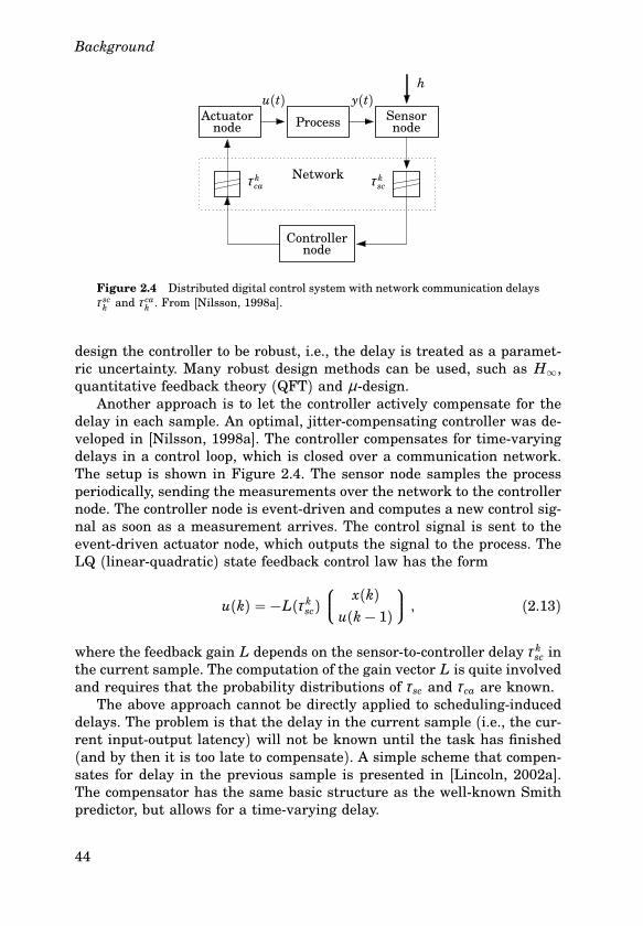
Figure 2.5 The inverted pendulum used in the Bluetooth network example. Thependulum is attached the end of a rotating arm.

Many other heuristic jitter compensation schemes have been suggested,e.g., [Hägglund, 1992; Albertos and Crespo, 1999; Marti et al., 2001]. Yetanother scheme (based on [Nilsson, 1998a]) is given in the following ex­ample.

EXAMPLE 2.1—INPUT­OUTPUT JITTER IN A BLUETOOTH NETWORKConsider a distributed control system where a rotating inverted pendulum(see Figure 2.5) should be controlled over a Bluetooth network. The exam­ple is taken from [Eker et al., 2001], where experiments on a laboratorysetup were reported.The objective of the control is to stabilize the pendulum in the upright

position by applying a torque to the rotating arm. The control designis based on a linearized, fourth­order model of the process. The full statevector (the arm and pendulum angles and their derivatives) is measurableon the process.The control system is configured according to the setup in Figure 2.4.

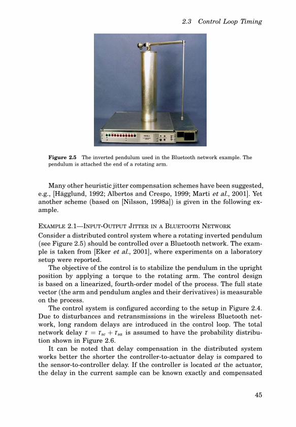
Due to disturbances and retransmissions in the wireless Bluetooth net­work, long random delays are introduced in the control loop. The totalnetwork delay τ = τ sc + τ sa is assumed to have the probability distribu­tion shown in Figure 2.6.It can be noted that delay compensation in the distributed system

works better the shorter the controller­to­actuator delay is compared tothe sensor­to­controller delay. If the controller is located at the actuator,the delay in the current sample can be known exactly and compensated

45

Background

20 30 40 50 600

0.2

0.4

τ [ms]

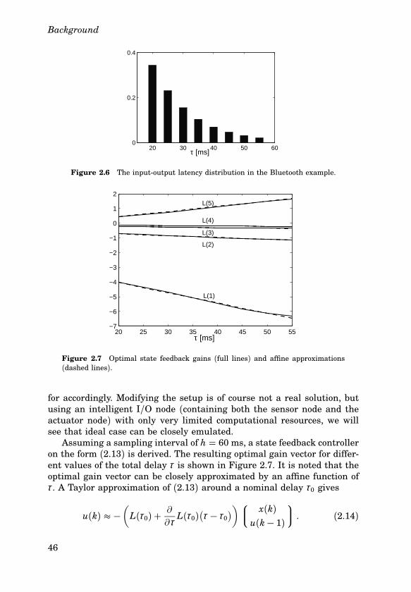
Figure 2.6 The input­output latency distribution in the Bluetooth example.

20 25 30 35 40 45 50 55−7

−6

−5

−4

−3

−2

−1

0

1

2

L(1)

L(2)

L(3)

L(4)

L(5)

τ [ms]

Figure 2.7 Optimal state feedback gains (full lines) and affine approximations(dashed lines).

for accordingly. Modifying the setup is of course not a real solution, butusing an intelligent I/O node (containing both the sensor node and theactuator node) with only very limited computational resources, we willsee that ideal case can be closely emulated.Assuming a sampling interval of h = 60 ms, a state feedback controller

on the form (2.13) is derived. The resulting optimal gain vector for differ­ent values of the total delay τ is shown in Figure 2.7. It is noted that theoptimal gain vector can be closely approximated by an affine function ofτ . A Taylor approximation of (2.13) around a nominal delay τ0 gives

u(k) � −(

L(τ0) + VVτL(τ0)

(

τ − τ0)

)

x(k)u(k− 1)

. (2.14)

46

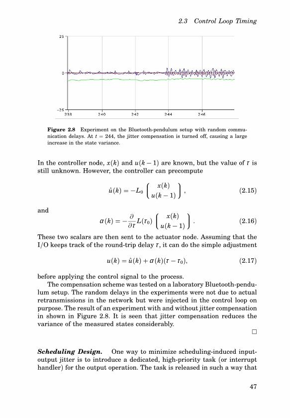
2.3 Control Loop Timing

Figure 2.8 Experiment on the Bluetooth­pendulum setup with random commu­nication delays. At t = 244, the jitter compensation is turned off, causing a largeincrease in the state variance.

In the controller node, x(k) and u(k− 1) are known, but the value of τ isstill unknown. However, the controller can precompute

u(k) = −L0

x(k)u(k− 1)

, (2.15)

and

α (k) = − VVτL(τ0)

x(k)u(k− 1)

. (2.16)

These two scalars are then sent to the actuator node. Assuming that theI/O keeps track of the round­trip delay τ , it can do the simple adjustment

u(k) = u(k) + α (k)(τ − τ0), (2.17)

before applying the control signal to the process.The compensation scheme was tested on a laboratory Bluetooth­pendu­

lum setup. The random delays in the experiments were not due to actualretransmissions in the network but were injected in the control loop onpurpose. The result of an experiment with and without jitter compensationin shown in Figure 2.8. It is seen that jitter compensation reduces thevariance of the measured states considerably.

Scheduling Design. One way to minimize scheduling­induced input­output jitter is to introduce a dedicated, high­priority task (or interrupthandler) for the output operation. The task is released in such a way that

47

Background

the latency between the input and the output is always constant. Theapproach has been suggested in various settings, e.g., [Locke, 1992; Kleinet al., 1993; Halang, 1993]. Disadvantages of the approach include a morecomplex implementation and more run­time overhead. Also, reducing jit­ter means increasing the average input­output latency. In [Balbastre et al.,2000], a design procedure that minimizes input­output jitter using high­priority input and output tasks is presented. Task attribute assignmentunder both FP and EDF scheduling is considered.Another option to reduce input­output jitter is, again, to use non­

preemptive scheduling. Given that the control algorithm has a constantexecution time, this will make the input­output latency constant. Thedrawback is that the scheduling design becomes more complicated.In [Baruah et al., 1999a], minimization of output jitter under EDF

scheduling is discussed. A list of properties that a “true” jitter minimiza­tion algorithm should fulfill is given: no new tasks should be introduced,outputs should not be suspended, etc. An algorithm is then suggestedwhere the utilizations of some tasks are increased in order to reduce thejitter.

Sampling Jitter

Control Design. As a rule of thumb, relative variations of the sam­pling interval that are smaller than ten percent of the nominal samplinginterval need not be compensated for. The simplest sampling jitter com­pensation methods are ad­hoc, but seem to work quite well, e.g., [Witten­mark and Åström, 1980; Albertos and Crespo, 1999; Marti et al., 2001].If the controller is based on a continuous­to­discrete approximation, theapproximation can be carried out in each sample, based on the previoussampling interval. The technique is illustrated on a PD (proportional­derivative) controller below.

EXAMPLE 2.2—SAMPLING JITTERConsider PD control of a DC servo. Let the servo be described by thecontinuous­time transfer function

G(s) = 1000s(s+ 1) . (2.18)

A good discrete­time implementation of the PD controller, which includesfiltering of the derivative part, is

P(k) = K (r(k) − y(k)),D(k) = adD(k− 1) + bd(y(k− 1) − y(k)),u(k) = P(k) + D(k),

(2.19)

48

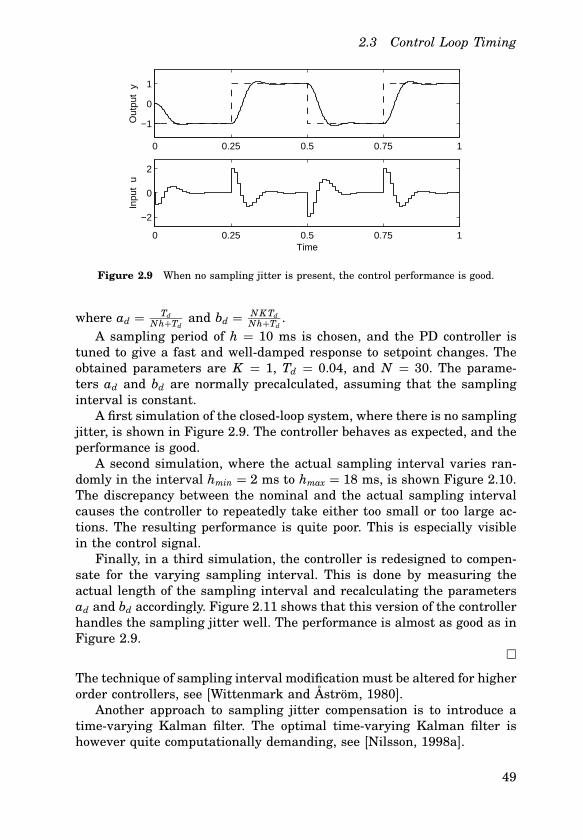
2.3 Control Loop Timing

0 0.25 0.5 0.75 1

−1

0

1

Out

put

y

0 0.25 0.5 0.75 1

−2

0

2

Inpu

t u

Time

Figure 2.9 When no sampling jitter is present, the control performance is good.

where ad = TdNh+Td and bd = NKTd

Nh+Td .A sampling period of h = 10 ms is chosen, and the PD controller is

tuned to give a fast and well­damped response to setpoint changes. Theobtained parameters are K = 1, Td = 0.04, and N = 30. The parame­ters ad and bd are normally precalculated, assuming that the samplinginterval is constant.A first simulation of the closed­loop system, where there is no sampling

jitter, is shown in Figure 2.9. The controller behaves as expected, and theperformance is good.A second simulation, where the actual sampling interval varies ran­

domly in the interval hmin = 2 ms to hmax = 18 ms, is shown Figure 2.10.The discrepancy between the nominal and the actual sampling intervalcauses the controller to repeatedly take either too small or too large ac­tions. The resulting performance is quite poor. This is especially visiblein the control signal.Finally, in a third simulation, the controller is redesigned to compen­

sate for the varying sampling interval. This is done by measuring theactual length of the sampling interval and recalculating the parametersad and bd accordingly. Figure 2.11 shows that this version of the controllerhandles the sampling jitter well. The performance is almost as good as inFigure 2.9.

The technique of sampling interval modification must be altered for higherorder controllers, see [Wittenmark and Åström, 1980].Another approach to sampling jitter compensation is to introduce a

time­varying Kalman filter. The optimal time­varying Kalman filter ishowever quite computationally demanding, see [Nilsson, 1998a].

49

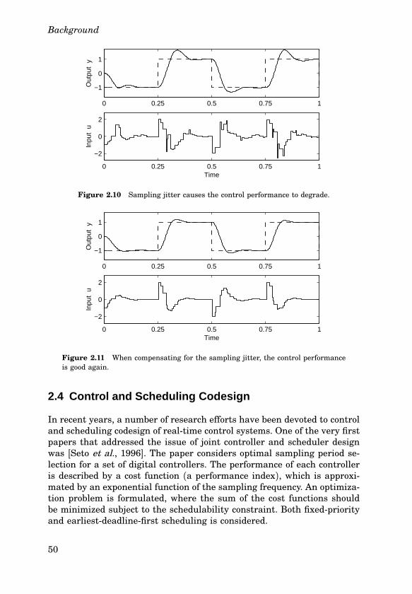
Background

0 0.25 0.5 0.75 1

−1

0

1

Out

put

y

0 0.25 0.5 0.75 1

−2

0

2

Inpu

t u

Time

Figure 2.10 Sampling jitter causes the control performance to degrade.

0 0.25 0.5 0.75 1

−1

0

1

Out

put

y

0 0.25 0.5 0.75 1

−2

0

2

Inpu

t u

Time

Figure 2.11 When compensating for the sampling jitter, the control performanceis good again.

2.4 Control and Scheduling Codesign

In recent years, a number of research efforts have been devoted to controland scheduling codesign of real­time control systems. One of the very firstpapers that addressed the issue of joint controller and scheduler designwas [Seto et al., 1996]. The paper considers optimal sampling period se­lection for a set of digital controllers. The performance of each controlleris described by a cost function (a performance index), which is approxi­mated by an exponential function of the sampling frequency. An optimiza­tion problem is formulated, where the sum of the cost functions shouldbe minimized subject to the schedulability constraint. Both fixed­priorityand earliest­deadline­first scheduling is considered.

50

2.4 Control and Scheduling Codesign

The previous paper does not consider the input­output latency in thecontrollers. An approach to joint optimization of sampling period andinput­output latency subject to performance specifications and schedula­bility constraints is presented in [Ryu et al., 1997; Ryu and Hong, 1998].The control performance is specified in terms of steady state error, over­shoot, rise time, and settling time. These performance parameters areexpressed as functions of the sampling period and the input­output la­tency. The goal of the optimization is to minimize the utilization of thetask set. A heuristic iterative algorithm is proposed for the optimizationof these parameters subject to schedulability constraints. The algorithmis based on the period calibration method (PCM) [Gerber et al., 1995] fordetermining the task attributes.Optimal sampling period selection for a set of linear­quadratic (LQ)

controllers is treated in [Eker et al., 2000]. Similar to [Seto et al., 1996],an optimization problem is formulated where the total performance ofthe controllers should be optimized subject to a schedulability constant.Analytical expressions for optimal LQ cost as a function of the samplinginterval are derived.The integration of static cyclic scheduling and optimal (LQ) control

is the topic of [Rehbinder and Sanfridson, 2000]. A number of processesshould be controlled by a set of state­feedback controllers. The perfor­mance of each controller is measured by a quadratic cost function. Acombinatorial optimization problem is formulated that, given a schedulelength, attempts to minimize the sum of the control costs. The solutioncontains the periodic task schedule as well as the state feedback gains ofthe controllers. A similar codesign problem is formulated in [Lincoln andBernhardsson, 2000]. There, the optimal switching sequence (i.e., sched­ule) for a set of controllers should be found. Unlike the previous paper,however, the obtained schedule is not necessarily periodic.In [Palopoli et al., 2002], sampling periods for a set of controllers should

be chosen such that a certain robustness measure is maximized. An opti­mization procedure is used to derive the gains of the controllers togetherwith the sampling periods, subject to a schedulability constraint. Themethod is limited in its applicability in that it only handles first­orderplants.A codesign method that assumes run­time scheduling decisions based

on current plant state information is presented in [Zhao and Zheng, 1999].There, the controller associated with the plant with the largest currentcontrol error is chosen for execution, while the other plants are fed zeros.An algorithm is given that determines the (static) state feedback laws tomeet a given performance specification.

51

3

Subtask Scheduling

3.1 Introduction

In the introductory chapter, it was shown that a naive implementation ofmultiple controllers on the same platform can introduce large amounts oflatency and jitter in the control loops. Listing 3.1 shows a straightforwardimplementation of a periodic control task. Each period, the input is read,the control algorithm is executed, and the output is written. In the bestcase, the controller has been designed to compensate for the computationaldelay in the control algorithm. When executing in the real­time system,additional, time­varying latency will be introduced by the task scheduling.Taken together, the latency and jitter degrade the control performance. Inthis chapter, we will show how the input­output latency can be reducedby more detailed scheduling analysis.It should be pointed out that input­output latency reduction is of out­

Listing 3.1 Naive implementation of a control loop. (The listings in this chapterare written in Modula­2 pseudo code.)

t := CurrentTime;

LOOP

ReadInput;

ControlAlgorithm;

WriteOutput;

t := t + h;

SleepUntil(t);

END;

52

3.1 Introduction

most importance. Even if the latency is fixed and known, delay compensa­tion can only recover part of the performance loss. This fact is illustratedby the following example:

EXAMPLE 3.1—MINIMUM­VARIANCE CONTROL OF AN INTEGRATORConsider minimum­variance control an integrator,

dx(t)dt

= u(t) + vc(t), (3.1)

where x is the state, u is the control signal, and vc is a continuous­timewhite noise process with zero mean and unit variance. A discrete­timecontroller is designed to minimize the continuous­time cost function

J = limT→∞

1T

∫ T

0x2(t) dt. (3.2)

Assuming an input­output latency of L, the cost for the optimal, delay­compensating controller is

J = 3+√3

6h+ L (� 0.79h+ L). (3.3)

(For details, see Appendix.) Note that the cost is very much affected bythe input­output latency. In this case, a one­sample latency (L = h) morethan doubles the value of the cost function compared to a controller withzero latency. To put it another way, a controller with a one­sample latencyneeds to execute more than twice as often as a controller with zero latencyto achieve the same performance.

Division into Calculate Output and Update State

A standard way to reduce the latency in a controller is to split the con­trol algorithm into two parts: Calculate Output and Update State (e.g.,[Åström and Wittenmark, 1997]), see Listing 3.2. Calculate Output con­tains only the operations immediately necessary to produce a control sig­nal, while the rest of the calculations are postponed to Update State.Consider for instance the implementation of a general linear controllerwritten in state­space form:

x(k+ 1) = Φx(k) + Γ y(k),u(k) = Cx(k) + Dy(k).

(3.4)

Here, only the calculation of Dy(k) (a scalar operation in the single­input,single­output case) and one addition needs to be performed in Calculate

53

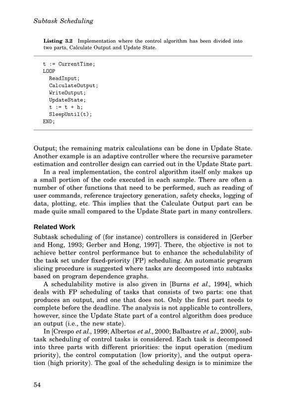
Subtask Scheduling

Listing 3.2 Implementation where the control algorithm has been divided intotwo parts, Calculate Output and Update State.

t := CurrentTime;

LOOP

ReadInput;

CalculateOutput;

WriteOutput;

UpdateState;

t := t + h;

SleepUntil(t);

END;

Output; the remaining matrix calculations can be done in Update State.Another example is an adaptive controller where the recursive parameterestimation and controller design can carried out in the Update State part.In a real implementation, the control algorithm itself only makes up

a small portion of the code executed in each sample. There are often anumber of other functions that need to be performed, such as reading ofuser commands, reference trajectory generation, safety checks, logging ofdata, plotting, etc. This implies that the Calculate Output part can bemade quite small compared to the Update State part in many controllers.

Related Work

Subtask scheduling of (for instance) controllers is considered in [Gerberand Hong, 1993; Gerber and Hong, 1997]. There, the objective is not toachieve better control performance but to enhance the schedulability ofthe task set under fixed­priority (FP) scheduling. An automatic programslicing procedure is suggested where tasks are decomposed into subtasksbased on program dependence graphs.A schedulability motive is also given in [Burns et al., 1994], which

deals with FP scheduling of tasks that consists of two parts: one thatproduces an output, and one that does not. Only the first part needs tocomplete before the deadline. The analysis is not applicable to controllers,however, since the Update State part of a control algorithm does producean output (i.e., the new state).In [Crespo et al., 1999; Albertos et al., 2000; Balbastre et al., 2000], sub­

task scheduling of control tasks is considered. Each task is decomposedinto three parts with different priorities: the input operation (mediumpriority), the control computation (low priority), and the output opera­tion (high priority). The goal of the scheduling design is to minimize the

54

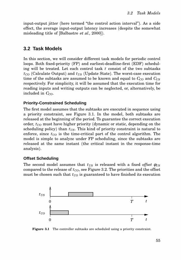
3.2 Task Models

input­output jitter (here termed “the control action interval”). As a sideeffect, the average input­output latency increases (despite the somewhatmisleading title of [Balbastre et al., 2000]).

3.2 Task Models

In this section, we will consider different task models for periodic controlloops. Both fixed­priority (FP) and earliest­deadline­first (EDF) schedul­ing will be treated. Let each control task τ consist of the two subtasksτCO (Calculate Output) and τUS (Update State). The worst­case executiontime of the subtasks are assumed to be known and equal to CCO and CUSrespectively. For simplicity, it will be assumed that the execution time forreading inputs and writing outputs can be neglected, or, alternatively, beincluded in CCO.

Priority-Constrained Scheduling

The first model assumes that the subtasks are executed in sequence usinga priority constraint, see Figure 3.1. In the model, both subtasks arereleased at the beginning of the period. To guarantee the correct executionorder, τCO must have higher priority (dynamic or static, depending on thescheduling policy) than τUS. This kind of priority constraint is natural toenforce, since τCO is the time­critical part of the control algorithm. Themodel is simple to analyze under FP scheduling, since the subtasks arereleased at the same instant (the critical instant in the response­timeanalysis).

Offset Scheduling

The second model assumes that τUS is released with a fixed offset φUScompared to the release of τCO, see Figure 3.2. The priorities and the offsetmust be chosen such that τCO is guaranteed to have finished its execution

0

0

T

T

τCO

τUSt

t

Figure 3.1 The controller subtasks are scheduled using a priority constraint.

55

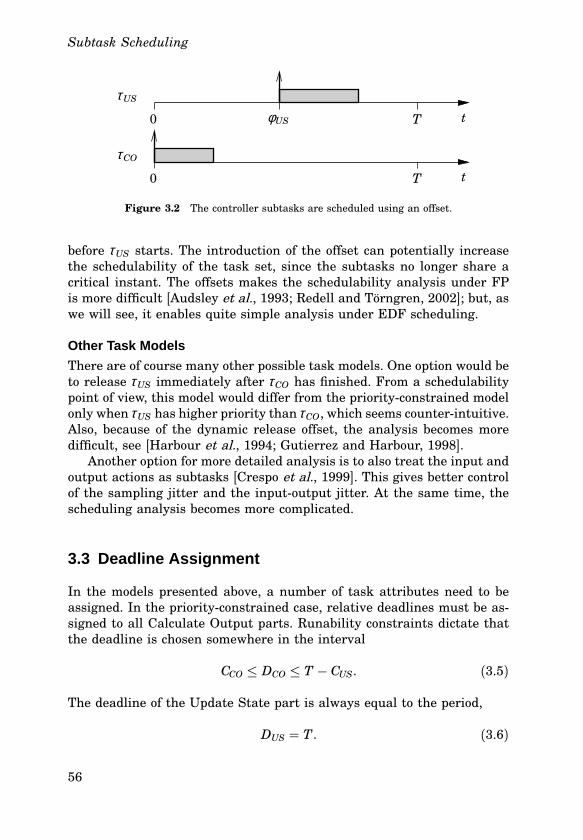
Subtask Scheduling

0

0

T

TφUS

τCO

τUSt

t

Figure 3.2 The controller subtasks are scheduled using an offset.

before τUS starts. The introduction of the offset can potentially increasethe schedulability of the task set, since the subtasks no longer share acritical instant. The offsets makes the schedulability analysis under FPis more difficult [Audsley et al., 1993; Redell and Törngren, 2002]; but, aswe will see, it enables quite simple analysis under EDF scheduling.

Other Task Models

There are of course many other possible task models. One option would beto release τUS immediately after τCO has finished. From a schedulabilitypoint of view, this model would differ from the priority­constrained modelonly when τUS has higher priority than τCO, which seems counter­intuitive.Also, because of the dynamic release offset, the analysis becomes moredifficult, see [Harbour et al., 1994; Gutierrez and Harbour, 1998].Another option for more detailed analysis is to also treat the input and

output actions as subtasks [Crespo et al., 1999]. This gives better controlof the sampling jitter and the input­output jitter. At the same time, thescheduling analysis becomes more complicated.

3.3 Deadline Assignment

In the models presented above, a number of task attributes need to beassigned. In the priority­constrained case, relative deadlines must be as­signed to all Calculate Output parts. Runability constraints dictate thatthe deadline is chosen somewhere in the interval

CCO ≤ DCO ≤ T − CUS. (3.5)

The deadline of the Update State part is always equal to the period,

DUS = T . (3.6)

56

3.3 Deadline Assignment

In the offset case, more attributes must be assigned. First, DCO must beselected according to (3.5). The offset φUS should be assigned somewherein the interval

DCO ≤ φUS ≤ T − CUS. (3.7)The relative deadline of Update State follows according to

DUS = T − φUS. (3.8)

Deadline Assignment under FP Scheduling

Both models above would in theory be applicable under both FP and EDFscheduling. However, from a designer’s perspective, we would like to usethe simplest schedulability analysis possible. For this reason, we will as­sume the priority­constrained model under FP scheduling and the offsetmodel under EDF scheduling.The ideal case under FP scheduling is when all Calculate Output parts

have higher priorities than all Update State parts. Unfortunately, sucha priority assignment might render the task set unschedulable. In caseswhere this approach does not work, the following iterative algorithm canbe used. Given a schedulable original task set, the algorithm attempts tominimize the deadlines of the Calculate Output parts while maintainingschedulability.

ALGORITHM 3.1

1. Start by assigning DUSi := Ti and DCOi := Ti − CUSi .2. Assign deadline­monotonic (DM) priorities Pi to all subtasks.3. Calculate the worst­case response times, RCOi , of the Calculate Out­put parts (see Section 2.2).

4. Assign new deadlines to the Calculate Output parts according toDCOi := RCOi .

5. Repeat from 2 until no further improvement in response times isobtained.

Some properties of the algorithm are formalized in the following theorem:

THEOREM 3.1Given a set a control tasks that is rate­monotonic (RM) schedulable, Al­gorithm 3.1 preserves schedulability in each iteration. Furthermore, thealgorithm terminates in a finite number of steps.

57

Subtask Scheduling

Proof. Schedulability in the first iteration: Since the original taskset is RM schedulable, each task must finish before its deadline Di =Ti. This implies that each Calculate Output parts must finish at leastbefore Ti − CUSi (otherwise the Update State part would not have timeto execute). Since the subtasks are schedulable under the RM deadlineassignment (i.e., both subtasks execute in sequence and with the samepriority), they must also be schedulable under the deadline­monotonic(DM) priority assignment, since that policy is optimal.Schedulability in the following iterations: After assigning new dead­

lines, the subtasks are obviously still schedulable with the old priorities(in fact, we will have RCOi = DCOi). The subtasks will be schedulable alsoafter the DM priority assignment since, again, that policy is optimal.Termination: After each iteration, the relative deadline of a Calculate

Output part can either decrease or remain the same. The relative priorityordering of the Calculate Output parts will never change, since a lowerpriority always implies a longer response time. Hence, the priority of aCalculate Output part can only increase, and the priority of an UpdateState part can only decrease. Since there are a finite number of priorityorderings, the priorities (and hence also the deadlines and the responsetimes) must converge after a finite number of steps.

Deadline Assignment under EDF

The priority­constrained model and the deadline assignment algorithmgiven above would also work under EDF scheduling. Unfortunately,response­time analysis is quite difficult under EDF. A simpler option isto use the offset model. With this model, deadlines can be assigned to thesubtasks such that the processor demand in each interval is equal to theutilization of the original task. The deadlines and the offsets are assignedaccording to

DCOi :=CCOi

CCOi + CUSiTi, (3.9)

and

DUSi :=CUSi

CCOi + CUSiTi, (3.10)

and the offset is chosen as φUSi = DCOi .Schedulability of the task set can be checked using the processor de­

mand approach (see Section 2.2). In the interval [0, φUSi ] the loadingfactor of the task is

CCOiφUSi

=CCOi + CUSi

Ti= CiTi

, (3.11)

58

3.4 Latency Analysis

and in the interval [φUSi , Ti] the loading factor is

CUSiTi − φUSi

=CCOi + CUSi

Ti= CiTi

. (3.12)

The loading factor (or utilization) of the original task was Ui = CiTi. The

subtasks are thus schedulable if and only if the original task was schedu­lable.

3.4 Latency Analysis

Once the subtask attribute assignment has been performed, response­time analysis can be applied to verify that the latencies in the controlloops have been reduced.

Latency Analysis under FP scheduling

Under fixed­priority scheduling, it is straightforward to derive bounds forthe sampling latency and the input­output latency.

Sampling Latency. Assuming that the sampling operation takes placeat the very start of the Calculate Output part, the maximum samplinglatency can be found by computing the worst­case response time of ahypothetical sampling task with a very short execution time and thesame priority as the original Calculate Output part. According to standardresponse­time analysis (see Section 2.2), the maximum sampling latencyfor task i is given by the smallest number Lmaxsi

> 0 that fulfills

Lmaxsi=

∑

j∈hp(i)

⌈

Lmaxsi

Tj

⌉

Cj . (3.13)

Here, hp(i) is the set of all subtasks or tasks with higher priority thanthe task under investigation.

Input­Output Latency. The maximum input­output latency occurswhen the task is released just prior to all other tasks in the system. Thetask has time to sample the plant but is then immediately preemptedby all higher­priority tasks. The maximum input­output latency of a con­troller is hence equal to the worst­case response time of the CalculateOutput part:

Lmaxioi= CCOi +

∑

j∈hp(i)

⌈

Lmaxioi

Tj

⌉

Cj . (3.14)

59

Subtask Scheduling

Similarly, the minimum input­output latency of a controller is equalto the best­case response time of the Calculate Output part. In the bestcase, the start of the task (i.e., the sampling operation) coincides with therelease of the task [Redell and Sanfridson, 2002]. According to the best­case response time analysis (see Section 2.2), the minimum input­outputlatency is thus given by

Lminioi= CbCOi +

∑

j∈hp(i)

⌈

Lminioi− TjTj

⌉

Cbj , (3.15)

where Cbi denotes the best­case execution time of task τ i.

Latency Analysis under EDF scheduling

Latency analysis under EDF can be performed using similar techniquesas those above. There are, however, no known formulas for the best­caseresponse times under EDF scheduling. An alternative to analysis is tasksimulation.Regarding the input­output latency, an interesting observation can be

made when comparing ordinary rate­monotonic scheduling to earliest­deadline­first scheduling (assuming Di = Ti for all tasks):

THEOREM 3.2Consider a set of control tasks implemented according to Listing 3.1 orListing 3.2. For each task, the maximum input­output latency under EDFscheduling is shorter than or equal to the corresponding maximum latencyunder RM scheduling.

Proof. Under RM scheduling, the maximum latency is given by (3.14).Now consider EDF scheduling. Assume that task τ i is released and then,possibly after some preemption, starts its execution. Once the task hasstarted, it can only be preempted by tasks with a shorter period. (Taskswith a longer period that arrive after τ i has started will have a laterdeadline than what τ i has.) Furthermore, τ i can only be preempted bytask instances that have an earlier deadline than what τ i has. This givesthe following upper bound on the input­output latency:

Lmaxioi= CCOi +

∑

j∈sp(i)

⌈

min(

Lmaxioi, Ti − Tj

)

Tj

⌉

Cj . (3.16)

Here, sp(i) is the set of tasks with shorter period than the task under in­vestigation. But this set is identical to the set hp(i) under rate­monotonicscheduling. Because of the min(⋅) operation, it follows that Lmaxioi

in (3.16)is less than or equal to Lmaxioi

in (3.14).

60

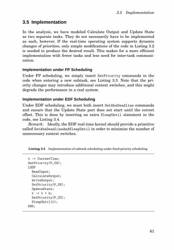
3.5 Implementation

3.5 Implementation

In the analysis, we have modeled Calculate Output and Update Stateas two separate tasks. They do not necessarily have to be implementedas such, however. If the real­time operating system supports dynamicchanges of priorities, only simple modifications of the code in Listing 3.2is needed to produce the desired result. This makes for a more efficientimplementation with fewer tasks and less need for inter­task communi­cation.

Implementation under FP Scheduling

Under FP scheduling, we simply insert SetPriority commands in thecode when entering a new subtask, see Listing 3.3. Note that the pri­ority changes may introduce additional context switches, and this mightdegrade the performance in a real system.

Implementation under EDF Scheduling

Under EDF scheduling, we must both insert SetAbsDeadline commandsand ensure that the Update State part does not start until the correctoffset. This is done by inserting an extra SleepUntil statement in thecode, see Listing 3.4.Remark: Ideally, the EDF real­time kernel should provide a primitive

called SetAbsDeadlineAndSleepUntil in order to minimize the number ofunnecessary context switches.

Listing 3.3 Implementation of subtask scheduling under fixed­priority scheduling.

t := CurrentTime;

SetPriority(P_CO);

LOOP

ReadInput;

CalculateOutput;

WriteOutput;

SetPriority(P_US);

UpdateState;

t := t + h;

SetPriority(P_CO);

SleepUntil(t);

END;

61

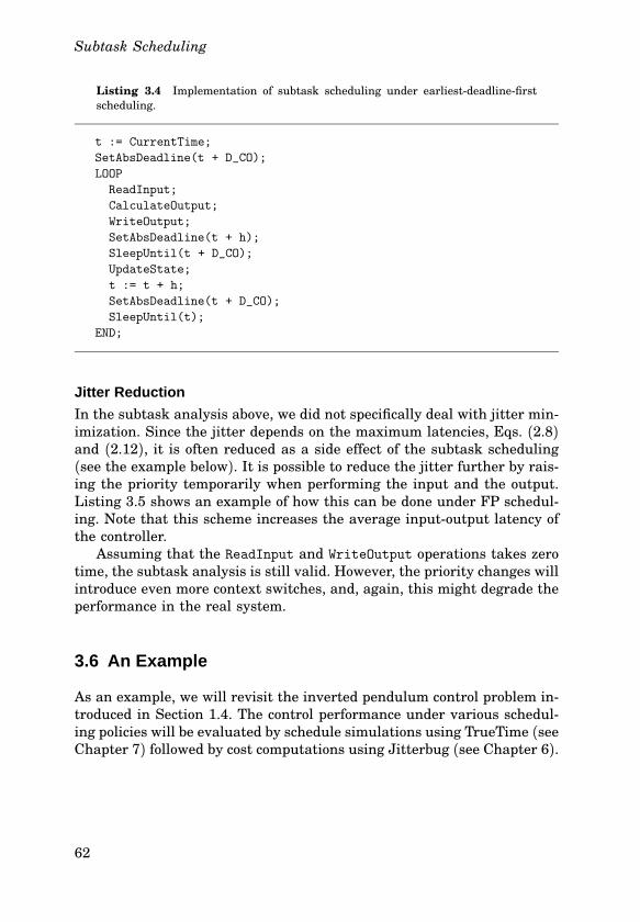
Subtask Scheduling

Listing 3.4 Implementation of subtask scheduling under earliest­deadline­firstscheduling.

t := CurrentTime;

SetAbsDeadline(t + D_CO);

LOOP

ReadInput;

CalculateOutput;

WriteOutput;

SetAbsDeadline(t + h);

SleepUntil(t + D_CO);

UpdateState;

t := t + h;

SetAbsDeadline(t + D_CO);

SleepUntil(t);

END;

Jitter Reduction

In the subtask analysis above, we did not specifically deal with jitter min­imization. Since the jitter depends on the maximum latencies, Eqs. (2.8)and (2.12), it is often reduced as a side effect of the subtask scheduling(see the example below). It is possible to reduce the jitter further by rais­ing the priority temporarily when performing the input and the output.Listing 3.5 shows an example of how this can be done under FP schedul­ing. Note that this scheme increases the average input­output latency ofthe controller.Assuming that the ReadInput and WriteOutput operations takes zero

time, the subtask analysis is still valid. However, the priority changes willintroduce even more context switches, and, again, this might degrade theperformance in the real system.

3.6 An Example

As an example, we will revisit the inverted pendulum control problem in­troduced in Section 1.4. The control performance under various schedul­ing policies will be evaluated by schedule simulations using TrueTime (seeChapter 7) followed by cost computations using Jitterbug (see Chapter 6).

62

3.6 An Example

Listing 3.5 Implementation of subtask scheduling with jitter reduction underfixed­priority scheduling.

t := CurrentTime;

SetPriority(HIGH);

LOOP

ReadInput;

SetPriority(P_CO);

CalculateOutput;

SetPriority(HIGH);

SleepUntil(t + D_CO);

WriteOutput;

SetPriority(P_US);

UpdateState;

t := t + h;

SetPriority(HIGH);

SleepUntil(t);

END;

Controller Design

Let each inverted pendulum be described by a linear transfer function,

G(s) = ω 20s2 − ω 20

, (3.17)

where ω 0 is the natural frequency of the pendulum. The different pendu­lum lengths, l = 0.1, 0.2, 0.3 m, correspond to different natural frequen­cies, ω 0 = 9.9, 7.0, 5.7 rad/s. It is assumed that the process is disturbedby a continuous­time white noise process with unit variance, and that themeasurements are disturbed by discrete­time noise with unit variance. AnLQG controller is designed to minimize the continuous­time cost function

J = limT→∞

1T

∫ T

0

y(t)u(t)

T

Q

y(t)u(t)

dt, (3.18)

where the weighting matrix Q is chosen as

Q =

1 0

0 0.002

.

The controller is designed (using the Jitterbug command lqgdesign) as­suming a constant input­output latency equal to the minimum input­output latency. The cost function (3.18) will also be used to evaluate theperformance of the controllers.

63

Subtask Scheduling

Table 3.1 First iteration of the deadline assignment algorithm.

T D C P R

τCO1 20 17 3 6 3

τUS1 20 20 4 5 7

τCO2 29 26 3 4 10

τUS2 29 29 4 3 14

τCO3 35 32 3 2 17

τUS3 35 35 4 1 28

Table 3.2 Third iteration of the deadline assignment algorithm.

T D C P R

τCO1 20 3 3 6 3

τUS1 20 20 4 3 13

τCO2 29 6 3 5 6

τUS2 29 29 4 2 17

τCO3 35 9 3 4 9

τUS3 35 35 4 1 28

Deadline Assignment

It is assumed that the execution time of the control algorithm is 7 ms.The Calculate Output part takes 3 ms, and the Update State part takes4 ms.

Fixed­Priority Scheduling Under FP scheduling, Algorithm 2.1 isused for assigning deadlines to the Calculate Output parts. In the firstiteration of the algorithm, we have the task set shown in Table 3.1. Inthe table, P denotes the priority of a subtask and R is the worst­caseresponse time (calculated according to (2.2)). After two more iterations,the values have converged, see Table 3.2. In this case, the end result isthat all Calculate Output parts have higher priority than all the UpdateState parts.

Earliest­Deadline­First Scheduling Under EDF scheduling, the sub­tasks are assigned relative deadlines according (3.9) and (3.10).

64

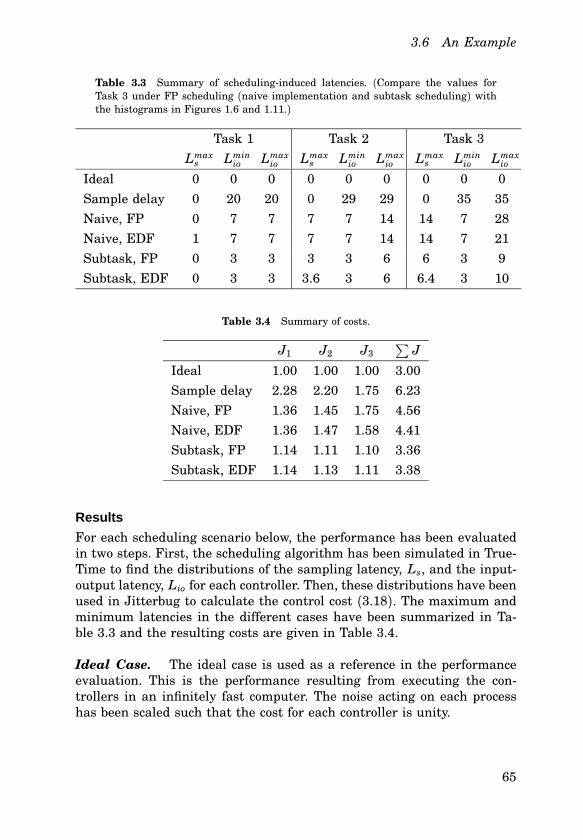
3.6 An Example

Table 3.3 Summary of scheduling­induced latencies. (Compare the values forTask 3 under FP scheduling (naive implementation and subtask scheduling) withthe histograms in Figures 1.6 and 1.11.)

Task 1 Task 2 Task 3

Lmaxs Lminio Lmaxio Lmaxs Lminio Lmaxio Lmaxs Lminio Lmaxio

Ideal 0 0 0 0 0 0 0 0 0

Sample delay 0 20 20 0 29 29 0 35 35

Naive, FP 0 7 7 7 7 14 14 7 28

Naive, EDF 1 7 7 7 7 14 14 7 21

Subtask, FP 0 3 3 3 3 6 6 3 9

Subtask, EDF 0 3 3 3.6 3 6 6.4 3 10

Table 3.4 Summary of costs.

J1 J2 J3∑

J

Ideal 1.00 1.00 1.00 3.00

Sample delay 2.28 2.20 1.75 6.23

Naive, FP 1.36 1.45 1.75 4.56

Naive, EDF 1.36 1.47 1.58 4.41

Subtask, FP 1.14 1.11 1.10 3.36

Subtask, EDF 1.14 1.13 1.11 3.38

Results

For each scheduling scenario below, the performance has been evaluatedin two steps. First, the scheduling algorithm has been simulated in True­Time to find the distributions of the sampling latency, Ls, and the input­output latency, Lio for each controller. Then, these distributions have beenused in Jitterbug to calculate the control cost (3.18). The maximum andminimum latencies in the different cases have been summarized in Ta­ble 3.3 and the resulting costs are given in Table 3.4.

Ideal Case. The ideal case is used as a reference in the performanceevaluation. This is the performance resulting from executing the con­trollers in an infinitely fast computer. The noise acting on each processhas been scaled such that the cost for each controller is unity.

65

Subtask Scheduling

Sample delay. In this implementation, there is a constant input­outputlatency of one sample for each controller. The input and output actionsare assumed to be performed in hardware, thus eliminating the jitter.Despite the exact delay compensation in the control design, the resultingperformance is poor.

Naive Implementation. In the naive implementation, the entire algo­rithm is computed before the output is written. This introduces a mini­mum input­output latency of 7 ms in all loops. The performance is com­parable under FP and EDF scheduling, but slightly better for Task 3under EDF scheduling. This is probably due to the shorter maximuminput­output latency of Task 3 under EDF scheduling (compare with The­orem 3.2).

Subtask Scheduling. Dividing the algorithm into Calculate Outputand Update state, the minimum input­output latency is decreased from7 to 3 ms. Under both FP and EDF scheduling, the maximum input­output latencies have been significantly reduced. The resulting controlperformance is quite close to the ideal case.

3.7 Conclusion

It has been shown how the performance of digital controllers can be im­proved by more detailed timing analysis. By scheduling the main parts ofa control algorithm as subtasks, it is possible to reduce the latencies in aset of control loops. The scheduling technique is simple to implement inordinary real­time operating systems.Subtask scheduling under EDF as suggested in this chapter is one of

the ideas behind the Control Server (see Chapter 5).One drawback with subtask scheduling is that more context switches

are introduced (see Figure 1.10). In the example above, the potentiallynegative effects of this were neglected. In Chapter 7, a more detailedsimulation is performed where the overhead due to context switches isaccounted for.

66

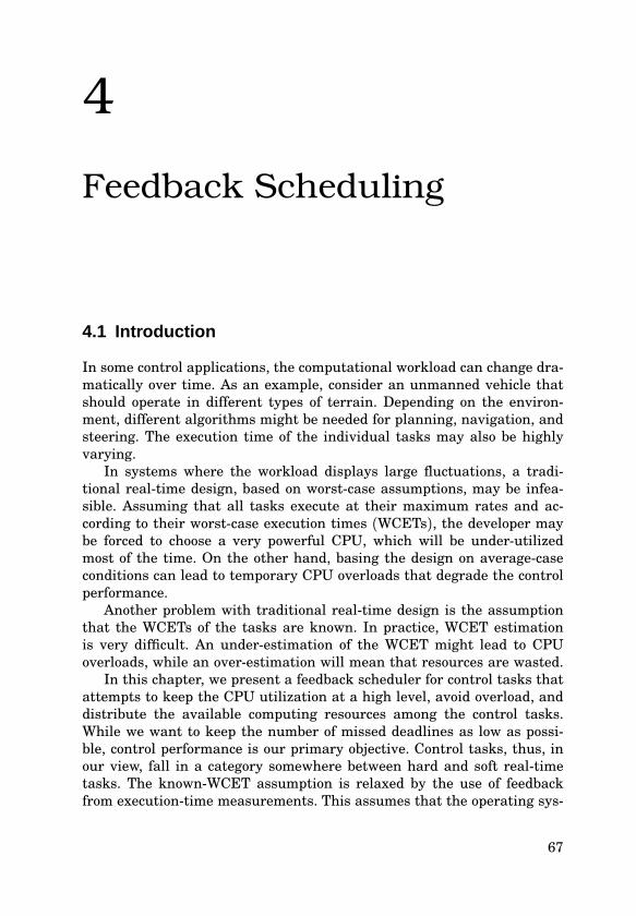
4

Feedback Scheduling

4.1 Introduction

In some control applications, the computational workload can change dra­matically over time. As an example, consider an unmanned vehicle thatshould operate in different types of terrain. Depending on the environ­ment, different algorithms might be needed for planning, navigation, andsteering. The execution time of the individual tasks may also be highlyvarying.In systems where the workload displays large fluctuations, a tradi­

tional real­time design, based on worst­case assumptions, may be infea­sible. Assuming that all tasks execute at their maximum rates and ac­cording to their worst­case execution times (WCETs), the developer maybe forced to choose a very powerful CPU, which will be under­utilizedmost of the time. On the other hand, basing the design on average­caseconditions can lead to temporary CPU overloads that degrade the controlperformance.Another problem with traditional real­time design is the assumption

that the WCETs of the tasks are known. In practice, WCET estimationis very difficult. An under­estimation of the WCET might lead to CPUoverloads, while an over­estimation will mean that resources are wasted.In this chapter, we present a feedback scheduler for control tasks that

attempts to keep the CPU utilization at a high level, avoid overload, anddistribute the available computing resources among the control tasks.While we want to keep the number of missed deadlines as low as possi­ble, control performance is our primary objective. Control tasks, thus, inour view, fall in a category somewhere between hard and soft real­timetasks. The known­WCET assumption is relaxed by the use of feedbackfrom execution­time measurements. This assumes that the operating sys­

67

Feedback Scheduling

tem supports measurements of task execution times. We also introducefeedforward to further improve the regulation of the utilization.Two simulation case studies are presented. First, we study a set of

hybrid controllers that switch mode during setpoint transitions. The com­putational resources are distributed among the tasks in an ad­hoc manner.In the second case study we consider scheduling of linear controllers thatcan be turned on and off. The CPU time is divided among the controllersin order to maximize a global cost function.

Related Work

In recent years, much research has been devoted to quality­of­service(QoS) aware real­time software, where the resource allocation in a systemis adjusted on­line in order to maximize the performance in some respect.In [Li and Nahrstedt, 1998] a general framework is proposed for control­ling the application requests for system resources using the amount ofallocated resources for feedback. It is shown that a PID controller can beused to bound the resource usage in a stable and fair way. In [Abeni andButtazzo, 1999], task models suitable for multimedia applications are de­fined. Two of these use PI control feedback to adjust the reserved fractionof CPU bandwidth. The resource allocation scheme Q­RAM is presented in[Rajkumar et al., 1997]. Several tasks are competing for finite resources,and each task is associated with a utility value, which is a function ofthe assigned resources. The system distributes the resources between thetasks to maximize the total utility of the system. In [Abdelzaher et al.,2000] a QoS renegotiation scheme is proposed as a way to allow grace­ful degradation in cases of overload, failures or violation of pre­runtimeassumptions. The mechanism permits clients to express, in their servicerequests, a range of QoS levels they can accept from the provider, and theperceived utility of receiving service at each of these levels. The approachis demonstrated in an automated flight­control system.Many scheduling techniques that allow QoS adaptation have been de­

veloped. An interesting mechanism for workload adjustments is given in[Buttazzo et al., 1998], where an elastic task model for periodic tasks ispresented. The relative sensitivities of tasks to period rescaling are ex­pressed in terms of elasticity coefficients. Schedulability analysis of thesystem under EDF scheduling is given. In [Gill et al., 1998], a mixedstatic/dynamic­priority scheduling approach for avionics systems is pre­sented. Each task is associated with a criticality parameter. In overloadsituations, tasks at the highest criticality level are allowed to executebefore other tasks. Similar ideas are used within the broader area ofvalue­based scheduling, e.g., [Burns et al., 2000].The idea of using feedback in scheduling has to some extent been previ­

ously used in general purpose operating systems, in the form of multi­level

68

4.1 Introduction

feedback queue scheduling [Kleinrock, 1970; Blevins and Ramamoorthy,1976; Potier et al., 1976]. However, this has mostly been done in an ad­hoc way. A more control­theoretical approach is taken in [Stankovic et al.,1999; Lu et al., 1999] that present a scheduling algorithm called Feed­back Control EDF (FC­EDF). A PID controller regulates the deadlinemiss­ratio for a set of soft real­time tasks with varying execution times,by adjusting their CPU utilization. It is assumed that tasks can changetheir CPU consumption by executing different versions of the same algo­rithm. An admission controller is used to accommodate larger changes inthe workload. In [Lu et al., 2000] the approach is extended. An additionalPID controller is added that instead controls the CPU utilization. Thetwo controllers are combined using a min­approach. The resulting hybridcontroller scheme, named FC­EDF2, gives good performance both duringsteady­state and under transient conditions. The framework is furthergeneralized in [Lu et al., 2002], where the feedback scheduler is brokendown in three parts: the monitor that measures the miss ratio and/orthe utilization, the control algorithm, and the QoS actuator that containsa QoS optimization algorithm to maximize the system value. In [Abeniet al., 2002], the problem of dynamically assigning bandwidths to a set ofconstant bandwidth servers [Abeni and Buttazzo, 1998] is analyzed. Theservers are modeled as discrete switched systems, and a feedback sched­uler that adjusts the server bandwidths is derived using hybrid controltheory.On­line adjustment of sampling periods in order to avoid CPU over­

loads is the topic of [Beccari et al., 1999]. A number of different rate­modulation algorithms suitable for rate­monotonic scheduling are given.A more control­theoretic approach to rate modulation is taken in [Shinand Meissner, 1999], where each controller is associated with a cost func­tion. During overloads, tasks may migrate between different CPUs in amultiprocessor in order to maximize the overall control performance.Adjustment of sampling rates is not the only way to achieve grace­

ful degradation in overloaded real­time control systems. Controllers thatare based on anytime algorithms allow a direct trade­off between theconsumed CPU time and the quality of control. A good example is model­predictive control (MPC), where the control signal is found by solving anoptimization problem in each sample. In the case of an overload, the op­timization may be terminated early and still produce acceptable results.In [Henriksson et al., 2002], scheduling of multiple MPC controllers isconsidered. Scheduling of anytime algorithms in avionics applications isdiscussed in [Agrawal et al., 2003], where the resources are dynamicallydistributed among the tasks in order to maximize the global QoS.Part of the work presented in this chapter is a continuation of the

work in [Eker et al., 2000], where a feedback scheduler for the special

69

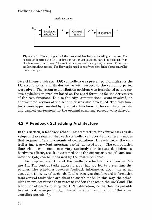
Feedback Scheduling

Usphi

mode changes

jobs ciFeedbackScheduler

ControlTasks Dispatcher

Figure 4.1 Block diagram of the proposed feedback scheduling structure. Thescheduler controls the CPU utilization to a given setpoint, based on feedback fromthe task execution times. The control is exercised through adjustment of the con­troller sampling periods. Feedforward is used to notify the scheduler about controllermode changes.

case of linear­quadratic (LQ) controllers was presented. Formulas for theLQ cost function and its derivative with respect to the sampling periodwere given. The resource distribution problem was formulated as a recur­sive optimization problem based on the exact formulas for the derivativesof the cost functions. Due to the high computational costs involved, anapproximate version of the scheduler was also developed. The cost func­tions were approximated by quadratic functions of the sampling periods,and explicit expressions for the optimal sampling periods were derived.

4.2 A Feedback Scheduling Architecture

In this section, a feedback scheduling architecture for control tasks is de­veloped. It is assumed that each controller can operate in different modesthat require different amounts of computations. In each mode, the con­troller has a nominal sampling period, denoted hnomi. The computationtime within each mode may vary randomly due to data dependencies,hardware effects, etc. It is assumed that the execution time of each taskinstance (job) can be measured by the real­time kernel.The proposed structure of the feedback scheduler is shown in Fig­

ure 4.1. The control tasks generate jobs that are fed to a run­time dis­patcher. The scheduler receives feedback information about the actualexecution time, ci, of each job. It also receives feedforward informationfrom control tasks that are about to switch mode. In this way, the sched­uler can pro­act rather than react to sudden changes in the workload. Thescheduler attempts to keep the CPU utilization, U , as close as possibleto a utilization setpoint, Usp. This is done by manipulation of the actualsampling periods, hi.

70

4.2 A Feedback Scheduling Architecture

Design Considerations

A number of design considerations exist. The utilization setpoint, Usp,must be chosen. The choice will depend on the scheduling policy of thedispatcher and on the sensitivity of the controllers to missed deadlines.A too low setpoint will give low resource utilization and poor control per­formance. A too high setpoint, on the other hand, may cause tasks to suf­fer from temporary overruns due to the varying execution times. Noticethat the well­known, guaranteed utilization bounds of 100% for deadline­driven scheduling and 69% for priority­driven scheduling [Liu and Lay­land, 1973] are not valid in this context, since the assumptions aboutknown, fixed WCETs and fixed periods are violated.The feedback scheduler itself will execute as a periodic task in the

system, and its period, hFBS, must be chosen. A shorter period will givegood control of the utilization but also consume much of the availableresources. A longer period will consume less resources but will make thescheduler respond slower to CPU load disturbances.The parameters in a digital controller typically depend on the sam­

pling interval. Hence, the controller must be aware of the current periodand adjust its parameters accordingly. On­line recalculations are often toocostly. Instead, parameters for a range of sampling periods can be calcu­lated off­line and stored in a table. Furthermore, the controller should berealized in a suitable form, such that the sampling period adjustments donot introduce transfer bumps.

Controlling the Utilization

The utilization control mechanism of the feedback scheduler consists oftwo parts: a utilization observer that estimates the current CPU utiliza­tion, and a resource allocator that divides the available resources amongthe tasks. In our architecture, the scheduler obtains execution­time esti­mates Ci from filtered job execution­time measurements,

Ci(k) = λ Ci(k− 1) + (1− λ)ci. (4.1)

Here, λ is a forgetting factor. Setting λ close to one results in a smooth, butslow estimate. A λ close to zero gives a faster, but more noisy execution­time estimate. Combining the execution­time estimates with the nominalsampling periods, the nominal utilization U can be estimated as

U =n

∑

i=1

Ci

hnomi. (4.2)

If U ≤ Usp, all tasks are allowed to execute with their nominal periods. Ifnot, the feedback scheduler assigns new sampling periods such that the

71

Feedback Scheduling

utilization setpoint is reached. This can be done in different ways. One op­tion is to apply simple linear rescaling of the task periods. Another optionis to derive optimal sampling periods for the controllers using control­theoretical arguments. Both options will be considered in the follwingsections.

Feedforward Information

The role of the feedforward information from the controllers to the feed­back scheduler is three­fold. First, the scheduler can react to suddenchanges in the workload by executing an extra time in connection witha mode change. The controller, which typically executes more frequentlythan the feedback scheduler, is responsible for signaling the scheduler assoon as a mode switch condition has been detected. If the mode changeis likely to increase the workload, and if the switching time itself is notcritical, the controller could delay the switch one or several sampling peri­ods while the scheduler recalculates the periods. Such a non­critical modeswitch could for instance be the result of an operator entering a new set­point for the controller.Second, the scheduler may need to keep track of the modes of the

controllers in order to assign suitable sampling periods. The controllercould communicate the new nominal sampling period at the mode switch,or the scheduler could keep a table of the nominal sampling periods forall the controller modes.Third, the mode information allows the scheduler to run separate

execution­time estimators in the different modes. The forgetting factorλ can then be chosen according to the execution­time variability withineach mode. At a mode change, the scheduler can immediately switch to thecurrent estimate in the new mode. This further improves the regulationof the utilization at the mode changes.

4.3 Case Study 1: Hybrid Controllers

As a first example of feedback scheduling, we will study the problemof scheduling a set of hybrid controllers that switch between differentinternal modes. The resource allocation is performed by simple rescalingof the nominal sampling periods.

A Hybrid Controller

A hybrid controller for the double­tank process, see Figure 4.2, was de­signed and implemented in [Eker and Malmborg, 1999]. The goal is tocontrol the level of the lower tank to a desired setpoint. The measurement

72

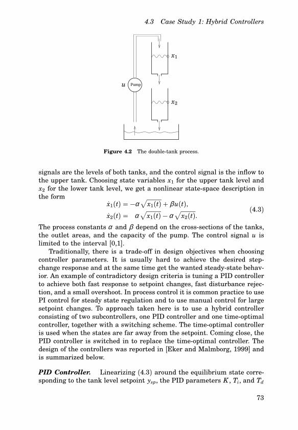
4.3 Case Study 1: Hybrid Controllers

Pump

x2

x1

u

Figure 4.2 The double­tank process.

signals are the levels of both tanks, and the control signal is the inflow tothe upper tank. Choosing state variables x1 for the upper tank level andx2 for the lower tank level, we get a nonlinear state­space description inthe form

x1(t) = −α√

x1(t) + βu(t),

x2(t) = α√

x1(t) − α√

x2(t).(4.3)

The process constants α and β depend on the cross­sections of the tanks,the outlet areas, and the capacity of the pump. The control signal u islimited to the interval [0,1].Traditionally, there is a trade­off in design objectives when choosing

controller parameters. It is usually hard to achieve the desired step­change response and at the same time get the wanted steady­state behav­ior. An example of contradictory design criteria is tuning a PID controllerto achieve both fast response to setpoint changes, fast disturbance rejec­tion, and a small overshoot. In process control it is common practice to usePI control for steady state regulation and to use manual control for largesetpoint changes. To approach taken here is to use a hybrid controllerconsisting of two subcontrollers, one PID controller and one time­optimalcontroller, together with a switching scheme. The time­optimal controlleris used when the states are far away from the setpoint. Coming close, thePID controller is switched in to replace the time­optimal controller. Thedesign of the controllers was reported in [Eker and Malmborg, 1999] andis summarized below.

PID Controller. Linearizing (4.3) around the equilibrium state corre­sponding to the tank level setpoint ysp, the PID parameters K , Ti, and Td

73

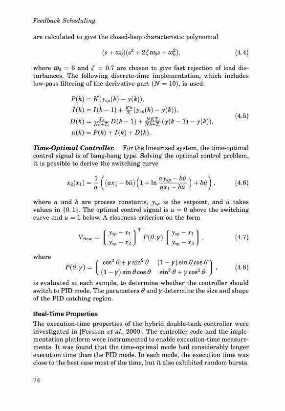
Feedback Scheduling

are calculated to give the closed­loop characteristic polynomial

(s+ ω 0)(s2 + 2ζ ω 0s+ ω 20), (4.4)

where ω 0 = 6 and ζ = 0.7 are chosen to give fast rejection of load dis­turbances. The following discrete­time implementation, which includeslow­pass filtering of the derivative part (N = 10), is used:

P(k) = K (ysp(k) − y(k)),

I(k) = I(k− 1) + KhTi

(ysp(k) − y(k)),

D(k) = TdNh+Td D(k− 1) + NKTd

Nh+Td (y(k− 1) − y(k)),

u(k) = P(k) + I(k) + D(k).

(4.5)

Time­Optimal Controller. For the linearized system, the time­optimalcontrol signal is of bang­bang type. Solving the optimal control problem,it is possible to derive the switching curve

x2(x1) = 1a

(

(

ax1 − bu)

(

1+ ln aysp − buax1 − bu

)

+ bu)

, (4.6)

where a and b are process constants, ysp is the setpoint, and u takesvalues in {0, 1}. The optimal control signal is u = 0 above the switchingcurve and u = 1 below. A closeness criterion on the form

Vclose =

ysp − x1ysp − x2

T

P(θ ,γ )

ysp − x1ysp − x2

, (4.7)

where

P(θ ,γ ) =

cos2 θ + γ sin2 θ (1− γ ) sinθ cosθ(1− γ ) sinθ cosθ sin2 θ + γ cos2 θ

, (4.8)

is evaluated at each sample, to determine whether the controller shouldswitch to PID mode. The parameters θ and γ determine the size and shapeof the PID catching region.

Real-Time Properties

The execution­time properties of the hybrid double­tank controller wereinvestigated in [Persson et al., 2000]. The controller code and the imple­mentation platform were instrumented to enable execution­time measure­ments. It was found that the time­optimal mode had considerably longerexecution time than the PID mode. In each mode, the execution time wasclose to the best case most of the time, but it also exhibited random bursts.

74

4.3 Case Study 1: Hybrid Controllers

(a) (b)

1.5 2 2.5 3 3.5 40

0.1

0.2

0.3

0.4

Execution time [ms]

Fre

quen

cy

9 10 11 12 13 14 150

0.1

0.2

0.3

0.4

Execution time [ms]

Fre

quen

cy

Figure 4.3 Assumed execution­time probability distributions in the hybrid con­troller: (a) PID mode, and (b) time­optimal mode.

For purposes of illustration, we here assume that the average executiontime in the PID mode is CPID = 2 ms and the average execution timein the time­optimal mode is COpt = 10 ms. The execution times of thealgorithms are assumed to vary randomly from invocation to invocationaccording to the probability distributions shown in Figure 4.3.

Experiments

Assume that three hybrid double­tank controllers should execute on thesame CPU. The double tanks have different physical parameters, result­ing in different rise times, Tr1, Tr2, Tr3 = 210, 180, 150 ms. Based onthe rise times, the controllers are assigned the nominal sampling inter­vals hnom1, hnom2, hnom3 = 21, 18, 15 ms. A controller has the same nom­inal sampling period in both modes. In the experiments, rate­monotonicscheduling is assumed, i.e., the task with the shortest period is assignedthe highest priority.A simulation of Task 1 executing in isolation is shown in Figure 4.4.

The process is disturbed by both input noise and measurement noise. Thecontroller displays good setpoint response and steady­state regulation. Itis seen that the CPU utilization is very low in PID mode, on averageCPID/hnom1 = 0.09. In the time­optimal mode, it is significantly higher, onaverage U = COpt/hnom1 = 0.45.Various scheduling approaches in the multiple­process case are eval­

uated by cosimulation of the scheduling algorithm and the process dy­namics using TrueTime (see Chapter 7). First, ordinary open­loop rate­monotonic scheduling is attempted. Next, a feedback scheduler is added tothe system. Finally, feedforward is introduced in the scheduler. A 4­secondsimulation cycle is constructed as follows. At time t = 0, all controllersstart in the PID mode. At t = 0.5, the worst­case scenario appears: all

75

Feedback Scheduling

0 0.5 1 1.5 2 2.5 3 3.5 4

0.1

0.15O

utpu

t

0 0.5 1 1.5 2 2.5 3 3.5 4

0

0.5

1

Inpu

t

0 0.5 1 1.5 2 2.5 3 3.5 40

1

2

Time

Util

izat

ion

Figure 4.4 Performance of Task 1 when running in isolation. The controller dis­plays good setpoint response and steady­state regulation. The CPU never becomesoverloaded.

controllers receive new setpoints and should switch to time­optimal mode.Following this, the controllers get new setpoints pairwise, and then oneby one. In each simulation, the behavior of Task 1, which is the lowest­priority controller, is plotted. Also plotted is the total CPU utilization,U =

∑

i ci/hi, where ci is the current execution time of task i, and hi isthe current period of task i.It is important to specify the behavior of the periodic tasks in the case

of missed deadlines. No matter when a task finishes, the next releasetime is set to the current release time plus the assigned period of thetask. Thus, a task that has missed many deadlines may have a releasetime that is far back in time compared to the actual starting time of thetask. This standard implementation of periodic tasks, e.g., [Liu, 2000],penalizes especially the low­priority tasks in the case of an overload.

Simulation Results

The simulation results under various scheduling strategies are presentedand discussed below.

Open­Loop Scheduling. We first consider open­loop scheduling, wherethe controllers are implemented as tasks with fixed periods equal to theirnominal sampling intervals. The simulation results are shown in Fig­ures 4.5 and 4.6.

76

4.3 Case Study 1: Hybrid Controllers

0 0.5 1 1.5 2 2.5 3 3.5 4

0.1

0.15

Out

put

0 0.5 1 1.5 2 2.5 3 3.5 4

0

0.5

1

Inpu

t

0 0.5 1 1.5 2 2.5 3 3.5 40

1

2

Time

Tot

alU

tiliz

atio

n

Figure 4.5 Performance of Task 1 under open­loop scheduling. The CPU is over­loaded during long intervals, and the controller cannot update its control signal veryoften. The result is poor control performance.

0.4 0.5 0.6 0.7 0.8 0.9

Tas

k 1

Time

0.4 0.5 0.6 0.7 0.8 0.9

Tas

k 2

0.4 0.5 0.6 0.7 0.8 0.9

Tas

k 3

Figure 4.6 Close­up of the schedule under open­loop scheduling. At t = 0.5, Task2 and 3 switch to time­optimal mode, and the CPU gets overloaded. As a result,Task 1 is preempted in a long interval.

The system easily becomes overloaded, since in the worst case, U =∑

i COpt/hnomi = 1.7. As seen in the schedule plot, Task 1 is completelyblocked in the interval t = [0.5, 0.9] because of preemption. The result isvery poor control performance.

77

Feedback Scheduling

Feedback Scheduling. Next, a feedback scheduler is introduced. Thescheduler is implemented as a high­priority task with a period of TFBS =100 ms. The utilization setpoint is set to Usp = 0.8. At each invocation,the feedback scheduler estimates the nominal utilization of the tasks bycomputing U =

∑

i Ci/hnomi. The λ factor in the execution­time estimationis set to λ = 0.9. If U > Usp, task periods are assigned according to thelinear rescaling

hi = hnomiU/Usp, (4.9)otherwise, the nominal sampling periods are used. The execution time ofthe feedback scheduler is assumed to be 2 ms. The simulation results areshown in Figures 4.7 and 4.8. The scheduler tries to keep the workloadclose to 0.8. However, there is a delay from a change in the utilizationuntil it is detected by the feedback scheduler. This results in CPU overloadpeaks at the mode change instants. For instance, Task 1 is blocked in theinterval t = [0.5, 0.58].

Feedback and Feedforward Scheduling. To increase the responsive­ness of the feedback scheduler, a feedforward mechanism is added. Whena task in PID mode detects a new setpoint, it notifies the feedback sched­uler, which is released immediately. The task periods are adjusted beforethe notifying task is allowed to continue to execute in the time­optimalmode. The execution­time estimation is improved by running separate es­timators in the different modes. A forgetting factor of λ = 0.9 is chosento give smooth estimates in both modes. The result is a more responsiveand accurate feedback scheduler. The simulation results are shown in Fig­ures 4.9 and 4.10. It is seen that the delay for Task 1 at the mode switcheshas been reduced, and that the control performance is slightly better.

Performance Evaluation and Summary. The performance of thecontrollers under different scheduling policies is evaluated using the cri­terion

Ji =∫ Tsim

0(yideali(t) − yi(t))2dt, (4.10)

where yideali is the process output when Task i is allowed to run unpre­empted at its nominal sampling interval and without any disturbances,while yi is the actual process output when Task i is running in the multi­tasking real­time system. Ten simulation cycles (Tsim = 40) are simulatedand the final accumulated costs for the controllers are summarized inTable 4.1.Under open­loop scheduling, Task 3 has a only very small cost, due

to the disturbances acting on the process. Task 2 suffers from some pre­emption from Task 3, which gives a small cost, while Task 1 is preemptedduring long intervals, which gives a very large final cost.

78

4.3 Case Study 1: Hybrid Controllers

0 0.5 1 1.5 2 2.5 3 3.5 4

0.1

0.15O

utpu

t

0 0.5 1 1.5 2 2.5 3 3.5 4

0

0.5

1

Inpu

t

0 0.5 1 1.5 2 2.5 3 3.5 40

1

2

Time

Tot

al

Util

izat

ion

Figure 4.7 Performance of Task 1 under feedback scheduling. The CPU is over­loaded in shorter intervals and the performance is better than under open­loopscheduling, cf. Figure 4.5.

0.4 0.5 0.6 0.7 0.8 0.9

Tas

k 1

Time

0.4 0.5 0.6 0.7 0.8 0.9

Tas

k 2

0.4 0.5 0.6 0.7 0.8 0.9

Tas

k 3

0.4 0.5 0.6 0.7 0.8 0.9

FB

S

Figure 4.8 Close­up of the schedule under feedback scheduling. At t = 0.5, Task 3switches to time­optimal mode, and the CPU gets overloaded. At t = 0.55, thefeedback scheduler rescales the task periods. But this allows Task 2 to switch totime­optimal mode, and the CPU gets overloaded again.

79

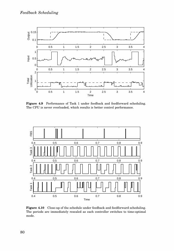
Feedback Scheduling

0 0.5 1 1.5 2 2.5 3 3.5 4

0.1

0.15O

utpu

t

0 0.5 1 1.5 2 2.5 3 3.5 4

0

0.5

1

Inpu

t

0 0.5 1 1.5 2 2.5 3 3.5 40

1

2

Time

Tot

alU

tiliz

atio

n

Figure 4.9 Performance of Task 1 under feedback and feedforward scheduling.The CPU is never overloaded, which results is better control performance.

0.4 0.5 0.6 0.7 0.8 0.9

Tas

k 1

Time

0.4 0.5 0.6 0.7 0.8 0.9

Tas

k 2

0.4 0.5 0.6 0.7 0.8 0.9

Tas

k 3

0.4 0.5 0.6 0.7 0.8 0.9

FB

S

Figure 4.10 Close­up of the schedule under feedback and feedforward scheduling.The periods are immediately rescaled as each controller switches to time­optimalmode.

80

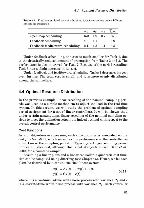
4.4 Optimal Resource Distribution

Table 4.1 Final accumulated costs for the three hybrid controllers under differentscheduling strategies.

J1 J2 J3∑

Ji

Open­loop scheduling 150 1.9 0.7 153

Feedback scheduling 4.6 1.1 1.2 6.9Feedback­feedforward scheduling 2.1 1.3 1.1 4.5

Under feedback scheduling, the cost is much smaller for Task 1, dueto the drastically reduced amount of preemption from Tasks 2 and 3. Theperformance is also improved for Task 2. Because of the period rescaling,Task 3 has a slight increase in its cost.Under feedback and feedforward scheduling, Tasks 1 decreases its cost

even further. The total cost is small, and it is more evenly distributedamong the controllers.

4.4 Optimal Resource Distribution

In the previous example, linear rescaling of the nominal sampling peri­ods was used as a simple mechanism to adjust the load in the real­timesystem. In this section, we will study the problem of optimal samplingperiod assignment for a set of linear controllers. It will be shown that,under certain assumptions, linear rescaling of the nominal sampling pe­riods to meet the utilization setpoint is indeed optimal with respect to theoverall control performance.

Cost Functions

As a quality­of­service measure, each sub­controller is associated with acost function J(h), which measures the performance of the controller asa function of the sampling period h. Typically, a longer sampling periodimplies a higher cost, although this is not always true (see [Eker et al.,2000] for a counter­example).Assuming a linear plant and a linear controller, a quadratic cost func­

tion can be computed using Jitterbug (see Chapter 6). Hence, we let eachplant be described by a continuous­time linear system,

x(t) = Ax(t) + Bu(t) + v(t),y(t) = Cx(t) + e(t),

(4.11)

where v is a continuous­time white noise process with variance R1 and eis a discrete­time white noise process with variance R2. Each controller

81

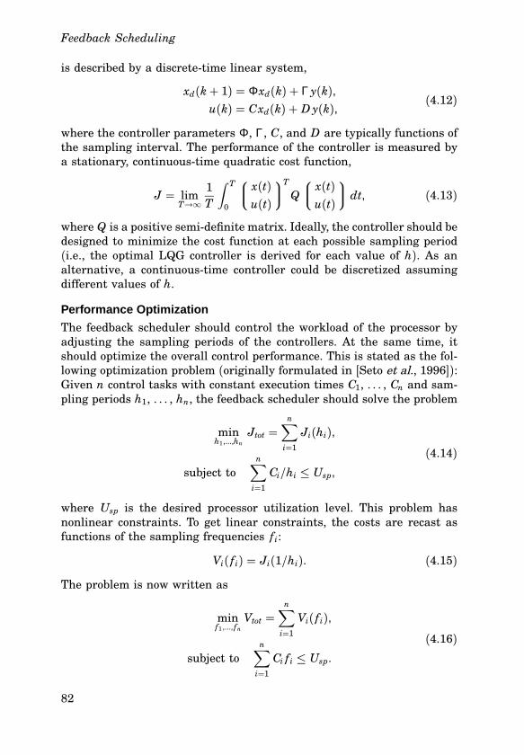
Feedback Scheduling

is described by a discrete­time linear system,

xd(k+ 1) = Φxd(k) + Γ y(k),u(k) = Cxd(k) + Dy(k),

(4.12)

where the controller parameters Φ, Γ, C, and D are typically functions ofthe sampling interval. The performance of the controller is measured bya stationary, continuous­time quadratic cost function,

J = limT→∞

1T

∫ T

0

x(t)u(t)

T

Q

x(t)u(t)

dt, (4.13)

where Q is a positive semi­definite matrix. Ideally, the controller should bedesigned to minimize the cost function at each possible sampling period(i.e., the optimal LQG controller is derived for each value of h). As analternative, a continuous­time controller could be discretized assumingdifferent values of h.

Performance Optimization

The feedback scheduler should control the workload of the processor byadjusting the sampling periods of the controllers. At the same time, itshould optimize the overall control performance. This is stated as the fol­lowing optimization problem (originally formulated in [Seto et al., 1996]):Given n control tasks with constant execution times C1, . . . , Cn and sam­pling periods h1, . . . , hn, the feedback scheduler should solve the problem

minh1,...,hn

Jtot =n

∑

i=1Ji(hi),

subject ton

∑

i=1Ci/hi ≤ Usp,

(4.14)

where Usp is the desired processor utilization level. This problem hasnonlinear constraints. To get linear constraints, the costs are recast asfunctions of the sampling frequencies f i:

Vi( f i) = Ji(1/hi). (4.15)

The problem is now written as

minf1 ,..., fn

Vtot =n

∑

i=1Vi( f i),

subject ton

∑

i=1Ci f i ≤ Usp.

(4.16)

82

4.4 Optimal Resource Distribution

Assuming that the functions V1( f1), . . . , Vn( fn) are decreasing and convex,the optimal frequencies f L

1 , . . . , fLn fulfill the Kuhn­Tucker conditions

VV f iVi( f L

i ) + λCi = 0,

λ(

Usp −n

∑

i=1Ci f

Li

)

= 0,

λ ≥ 0,

(4.17)

where λ is the Lagrange multiplier (see, e.g., [Fletcher, 1987]).Solving the optimization problem exactly can be very time­consuming.

Evaluating a cost function for a single sampling frequency involves a largeamount of computations. If the resource allocation problem is to be solvedby an on­line optimizer, the cost functions for the plants must be com­puted off­line and then approximated by simpler functions. A quadraticapproximation was suggested in [Eker et al., 2000]. Here, we also presenta linear approximation. It is shown that the solution to the approximatedproblem can in both cases be interpreted as a simple linear rescaling ofthe nominal sampling periods.

Quadratic Approximation. Assume that the cost functions can beapproximated by

Ji(hi) = α i + β ih2i , (4.18)or, equivalently,

Vi( f i) = α i + β i(1/ f i)2. (4.19)Applying the Kuhn­Tucker conditions (4.17) yields the explicit solution

f Li =

(β iCi

)1/3 Usp∑nj=1 C

2/3j β 1/3j

. (4.20)

Notice that the constants α i can be disregarded, i.e., it is sufficient toestimate the curvature of the cost functions.

Linear Approximation. Assume that the cost functions can be ap­proximated by

Ji(hi) = α i + γ ihi, (4.21)or, equivalently,

Vi( f i) = α i + γ i/ f i. (4.22)

83

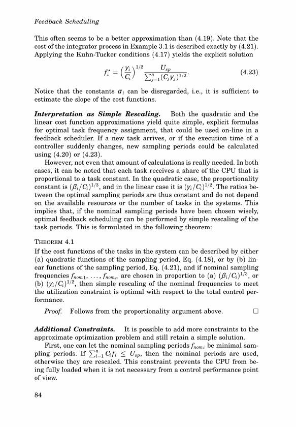
Feedback Scheduling

This often seems to be a better approximation than (4.19). Note that thecost of the integrator process in Example 3.1 is described exactly by (4.21).Applying the Kuhn­Tucker conditions (4.17) yields the explicit solution

f Li =

( γ iCi

)1/2 Usp∑nj=1(Cjγ j)1/2

. (4.23)

Notice that the constants α i can be disregarded, i.e., it is sufficient toestimate the slope of the cost functions.

Interpretation as Simple Rescaling. Both the quadratic and thelinear cost function approximations yield quite simple, explicit formulasfor optimal task frequency assignment, that could be used on­line in afeedback scheduler. If a new task arrives, or if the execution time of acontroller suddenly changes, new sampling periods could be calculatedusing (4.20) or (4.23).However, not even that amount of calculations is really needed. In both

cases, it can be noted that each task receives a share of the CPU that isproportional to a task constant. In the quadratic case, the proportionalityconstant is (β i/Ci)1/3, and in the linear case it is (γ i/Ci)1/2. The ratios be­tween the optimal sampling periods are thus constant and do not dependon the available resources or the number of tasks in the systems. Thisimplies that, if the nominal sampling periods have been chosen wisely,optimal feedback scheduling can be performed by simple rescaling of thetask periods. This is formulated in the following theorem:

THEOREM 4.1If the cost functions of the tasks in the system can be described by either(a) quadratic functions of the sampling period, Eq. (4.18), or by (b) lin­ear functions of the sampling period, Eq. (4.21), and if nominal samplingfrequencies fnom1, . . . , fnomn are chosen in proportion to (a) (β i/Ci)1/3, or(b) (γ i/Ci)1/2, then simple rescaling of the nominal frequencies to meetthe utilization constraint is optimal with respect to the total control per­formance.

Proof. Follows from the proportionality argument above.

Additional Constraints. It is possible to add more constraints to theapproximate optimization problem and still retain a simple solution.First, one can let the nominal sampling periods fnomi be minimal sam­

pling periods. If∑ni=1 Ci f i ≤ Usp, then the nominal periods are used,

otherwise they are rescaled. This constraint prevents the CPU from be­ing fully loaded when it is not necessary from a control performance pointof view.

84

4.5 Case Study 2: Linear Controllers

Second, one can impose maximum sampling periods to some tasks.This leads to an iterative solution (linear programming), where the re­maining tasks are rescaled until all constraints are met.

4.5 Case Study 2: Linear Controllers

As a second example we study the problem of simultaneously stabiliz­ing four inverted pendulums. Again, different scheduling approaches areevaluated by cosimulation of the scheduler, the control tasks, and the pen­dulums. By simulating the execution of the tasks, the effects of latencyand jitter (due to varying execution times and scheduling) on the controlperformance are also captured in the results.

Plants and Controllers

Similar to the example in Section 3.6, each inverted pendulum is describedby the system

G(s) = ω 20s2 − ω 20

, (4.24)

where ω 0 is the natural frequency of the pendulum. The pendulums havedifferent lengths that correspond to different natural frequencies, ω 0 =10, 13.3, 16.6, 20 rad/s. The processes are disturbed by continuous­timeinput noise with the variance R1 = 1/ω 0 and discrete­time measurementnoise with the variance R2 = 10−4.Discrete­time LQG­controllers for the plants are designed to minimize

the continuous­time cost function

J = limT→∞

1T

∫ T

0

(

y2(t) + u2(t))

dt. (4.25)

The costs functions for the four pendulums as functions of the samplingperiod are computed using Jitterbug (see Chapter 6) and are shown inFigure 4.11. It is seen that the cost functions can be reasonably wellapproximated by linear functions,

Ji(h) = α i + γ ih. (4.26)

The estimated slopes of the cost functions are γ = 43, 67, 95, 127. It can benoted that, the higher the natural frequency of the pendulum is, the moresensitive the controller is towards an increase in the sampling period. Thisis quite intuitive.Nominal sampling periods are chosen according to the solution of the

performance optimization problem and according to the rule of thumb

85

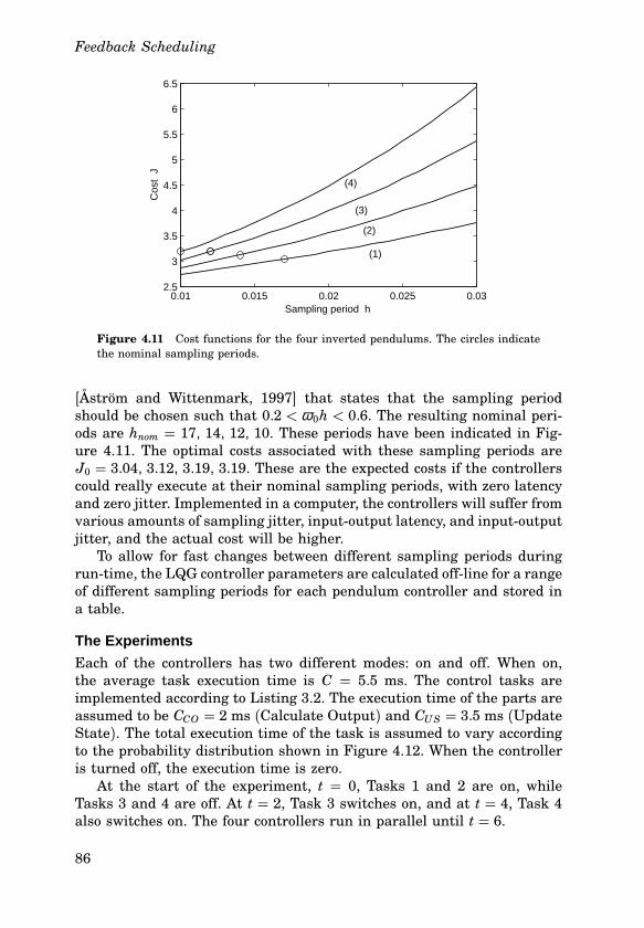
Feedback Scheduling

0.01 0.015 0.02 0.025 0.032.5

3

3.5

4

4.5

5

5.5

6

6.5

Sampling period h

Cos

t J

(1)

(2)

(3)

(4)

Figure 4.11 Cost functions for the four inverted pendulums. The circles indicatethe nominal sampling periods.

[Åström and Wittenmark, 1997] that states that the sampling periodshould be chosen such that 0.2 < ω 0h < 0.6. The resulting nominal peri­ods are hnom = 17, 14, 12, 10. These periods have been indicated in Fig­ure 4.11. The optimal costs associated with these sampling periods areJ0 = 3.04, 3.12, 3.19, 3.19. These are the expected costs if the controllerscould really execute at their nominal sampling periods, with zero latencyand zero jitter. Implemented in a computer, the controllers will suffer fromvarious amounts of sampling jitter, input­output latency, and input­outputjitter, and the actual cost will be higher.To allow for fast changes between different sampling periods during

run­time, the LQG controller parameters are calculated off­line for a rangeof different sampling periods for each pendulum controller and stored ina table.

The Experiments

Each of the controllers has two different modes: on and off. When on,the average task execution time is C = 5.5 ms. The control tasks areimplemented according to Listing 3.2. The execution time of the parts areassumed to be CCO = 2 ms (Calculate Output) and CUS = 3.5 ms (UpdateState). The total execution time of the task is assumed to vary accordingto the probability distribution shown in Figure 4.12. When the controlleris turned off, the execution time is zero.At the start of the experiment, t = 0, Tasks 1 and 2 are on, while

Tasks 3 and 4 are off. At t = 2, Task 3 switches on, and at t = 4, Task 4also switches on. The four controllers run in parallel until t = 6.

86

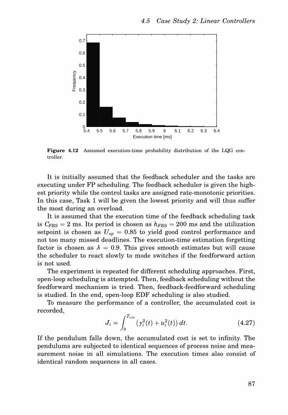
4.5 Case Study 2: Linear Controllers

5.4 5.5 5.6 5.7 5.8 5.9 6 6.1 6.2 6.3 6.40

0.1

0.2

0.3

0.4

0.5

0.6

0.7

Execution time [ms]

Fre

quen

cy

Figure 4.12 Assumed execution­time probability distribution of the LQG con­troller.

It is initially assumed that the feedback scheduler and the tasks areexecuting under FP scheduling. The feedback scheduler is given the high­est priority while the control tasks are assigned rate­monotonic priorities.In this case, Task 1 will be given the lowest priority and will thus sufferthe most during an overload.It is assumed that the execution time of the feedback scheduling task

is CFBS = 2 ms. Its period is chosen as hFBS = 200 ms and the utilizationsetpoint is chosen as Usp = 0.85 to yield good control performance andnot too many missed deadlines. The execution­time estimation forgettingfactor is chosen as λ = 0.9. This gives smooth estimates but will causethe scheduler to react slowly to mode switches if the feedforward actionis not used.The experiment is repeated for different scheduling approaches. First,

open­loop scheduling is attempted. Then, feedback scheduling without thefeedforward mechanism is tried. Then, feedback­feedforward schedulingis studied. In the end, open­loop EDF scheduling is also studied.To measure the performance of a controller, the accumulated cost is

recorded,

Ji =∫ Tsim

0

(

y2i (t) + u2i (t))

dt. (4.27)

If the pendulum falls down, the accumulated cost is set to infinity. Thependulums are subjected to identical sequences of process noise and mea­surement noise in all simulations. The execution times also consist ofidentical random sequences in all cases.

87

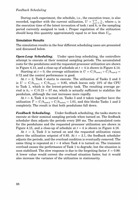
Feedback Scheduling

During each experiment, the schedule, i.e., the execution trace, is alsorecorded, together with the current utilization, U =

∑ni=1

cihi, where ci is

the execution time of the latest invocation of task i and hi is the samplingperiod currently assigned to task i. Proper regulation of the utilizationshould keep this quantity approximately equal to or less than Usp.

Simulation Results

The simulation results in the four different scheduling cases are presentedand discussed below.

Open­Loop Scheduling. Under open­loop scheduling, the controllersattempt to execute at their nominal sampling periods. The accumulatedcosts for the pendulums and the requested processor utilization are shownin Figure 4.13, and a close­up of schedule at t = 4 is shown in Figure 4.14.Starting at t = 0, the average utilization is U = C/hnom1 + C/hnom2 =

0.72 and the control performance is good.At t = 2, Task 3 starts to execute. The utilization of Tasks 2 and 3

is U = C/hnom1 + C/hnom2 = 0.85, which leaves only 15% of the CPUto Task 1, which is the lowest­priority task. The resulting average pe­riod is h1 = C/0.15 = 37 ms, which is actually sufficient to stabilize thependulum, although the cost increases more rapidly.At t = 4, Task 4 is turned on. Tasks 3 and 4 taken together have the

utilization T = C/hnom3 + C/hnom4 = 1.01, and this blocks Tasks 1 and 2completely. The result is that both pendulums fall down.

Feedback Scheduling. Under feedback scheduling, the tasks starts toexecute at their nominal sampling periods when turned on. The feedbackscheduler then adjusts the periods every 200 ms. The accumulated costsfor the pendulums and the requested processor utilization are shown inFigure 4.15, and a close­up of schedule at t = 4 is shown in Figure 4.16.At t = 2, Task 3 is turned on and the requested utilization raises

above the utilization setpoint of 0.85. At t = 2.1, the feedback scheduleradjusts the periods, and the overload condition is eventually removed. Thesame thing is repeated at t = 4 when Task 4 is turned on. The transientoverload causes the performance of Task 1 to degrade, but the situation issoon stabilized. The slow response is due to the forgetting factor λ = 0.99.A lower value would correct the overload situation faster, but it wouldalso increase the variance of the utilization in stationarity.

88

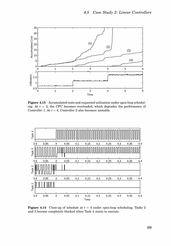
4.5 Case Study 2: Linear Controllers

0 1 2 3 4 5 60

5

10

15

20

25

30

35

Time

Acc

umul

ated

Cos

t

0 1 2 3 4 5 60.5

1

1.5

2

Time

Util

izat

ion

(1) (2)

(3)

(4)

Figure 4.13 Accumulated costs and requested utilization under open­loop schedul­ing. At t = 2, the CPU becomes overloaded, which degrades the performance ofController 1. At t = 4, Controller 2 also becomes unstable.

3.9 3.95 4 4.05 4.1 4.15 4.2 4.25 4.3 4.35 4.4

Tas

k 1

Time

3.9 3.95 4 4.05 4.1 4.15 4.2 4.25 4.3 4.35 4.4

Tas

k 2

3.9 3.95 4 4.05 4.1 4.15 4.2 4.25 4.3 4.35 4.4

Tas

k 3

3.9 3.95 4 4.05 4.1 4.15 4.2 4.25 4.3 4.35 4.4

Tas

k 4

Figure 4.14 Close­up of schedule at t = 4 under open­loop scheduling. Tasks 2and 3 become completely blocked when Task 4 starts to execute.

89

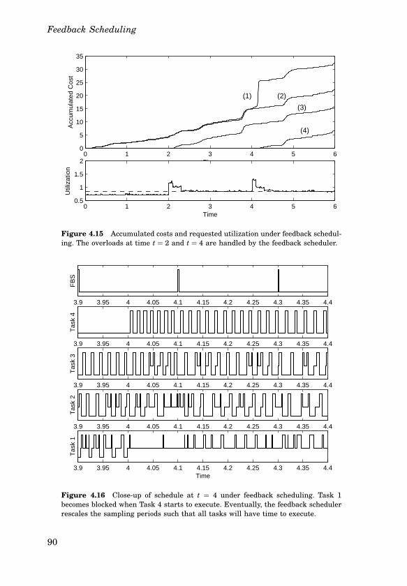
Feedback Scheduling

0 1 2 3 4 5 60

5

10

15

20

25

30

35

Time

Acc

umul

ated

Cos

t

0 1 2 3 4 5 60.5

1

1.5

2

Util

izat

ion

Time

(1) (2)

(3)

(4)

Figure 4.15 Accumulated costs and requested utilization under feedback schedul­ing. The overloads at time t = 2 and t = 4 are handled by the feedback scheduler.

3.9 3.95 4 4.05 4.1 4.15 4.2 4.25 4.3 4.35 4.4

Tas

k 1

Time

3.9 3.95 4 4.05 4.1 4.15 4.2 4.25 4.3 4.35 4.4

Tas

k 2

3.9 3.95 4 4.05 4.1 4.15 4.2 4.25 4.3 4.35 4.4

Tas

k 3

3.9 3.95 4 4.05 4.1 4.15 4.2 4.25 4.3 4.35 4.4

Tas

k 4

3.9 3.95 4 4.05 4.1 4.15 4.2 4.25 4.3 4.35 4.4

FB

S

Figure 4.16 Close­up of schedule at t = 4 under feedback scheduling. Task 1becomes blocked when Task 4 starts to execute. Eventually, the feedback schedulerrescales the sampling periods such that all tasks will have time to execute.

90

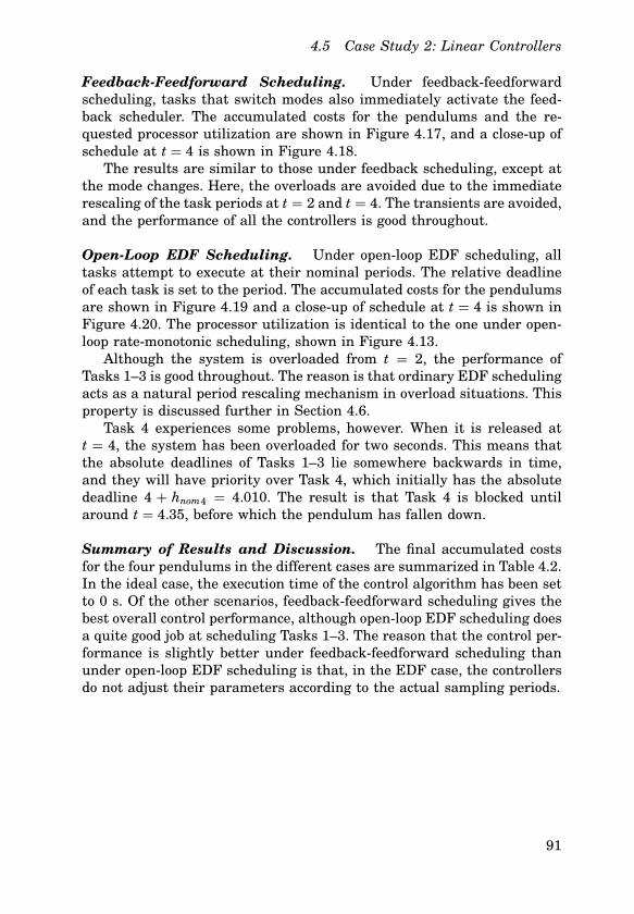
4.5 Case Study 2: Linear Controllers

Feedback­Feedforward Scheduling. Under feedback­feedforwardscheduling, tasks that switch modes also immediately activate the feed­back scheduler. The accumulated costs for the pendulums and the re­quested processor utilization are shown in Figure 4.17, and a close­up ofschedule at t = 4 is shown in Figure 4.18.The results are similar to those under feedback scheduling, except at

the mode changes. Here, the overloads are avoided due to the immediaterescaling of the task periods at t = 2 and t = 4. The transients are avoided,and the performance of all the controllers is good throughout.

Open­Loop EDF Scheduling. Under open­loop EDF scheduling, alltasks attempt to execute at their nominal periods. The relative deadlineof each task is set to the period. The accumulated costs for the pendulumsare shown in Figure 4.19 and a close­up of schedule at t = 4 is shown inFigure 4.20. The processor utilization is identical to the one under open­loop rate­monotonic scheduling, shown in Figure 4.13.Although the system is overloaded from t = 2, the performance of

Tasks 1–3 is good throughout. The reason is that ordinary EDF schedulingacts as a natural period rescaling mechanism in overload situations. Thisproperty is discussed further in Section 4.6.Task 4 experiences some problems, however. When it is released at

t = 4, the system has been overloaded for two seconds. This means thatthe absolute deadlines of Tasks 1–3 lie somewhere backwards in time,and they will have priority over Task 4, which initially has the absolutedeadline 4 + hnom4 = 4.010. The result is that Task 4 is blocked untilaround t = 4.35, before which the pendulum has fallen down.

Summary of Results and Discussion. The final accumulated costsfor the four pendulums in the different cases are summarized in Table 4.2.In the ideal case, the execution time of the control algorithm has been setto 0 s. Of the other scenarios, feedback­feedforward scheduling gives thebest overall control performance, although open­loop EDF scheduling doesa quite good job at scheduling Tasks 1–3. The reason that the control per­formance is slightly better under feedback­feedforward scheduling thanunder open­loop EDF scheduling is that, in the EDF case, the controllersdo not adjust their parameters according to the actual sampling periods.

91

Feedback Scheduling

0 1 2 3 4 5 60

5

10

15

20

25

30

35

Time

Acc

umul

ated

Cos

t

0 1 2 3 4 5 60.5

1

1.5

2

Util

izat

ion

Time

(1)

(2) (3)

(4)

Figure 4.17 Accumulated costs and requested utilization under feedback­feedforward scheduling. The feedforward action makes it possible to avoid CPUoverloads completely. The result is better control performance.

3.9 3.95 4 4.05 4.1 4.15 4.2 4.25 4.3 4.35 4.4

Tas

k 1

Time

3.9 3.95 4 4.05 4.1 4.15 4.2 4.25 4.3 4.35 4.4

Tas

k 2

3.9 3.95 4 4.05 4.1 4.15 4.2 4.25 4.3 4.35 4.4

Tas

k 3

3.9 3.95 4 4.05 4.1 4.15 4.2 4.25 4.3 4.35 4.4

Tas

k 4

3.9 3.95 4 4.05 4.1 4.15 4.2 4.25 4.3 4.35 4.4

FB

S

Figure 4.18 Close­up of schedule at t = 4 under feedback­feedforward scheduling.When Task 4 is turned on at t = 4, the feedback scheduler is immediately released.

92

4.5 Case Study 2: Linear Controllers

0 1 2 3 4 5 60

5

10

15

20

25

30

35

Time

Acc

umul

ated

Cos

t

0 1 2 3 4 5 60.5

1

1.5

2

Util

izat

ion

Time

(1)

(2)

(3)

(4)

Figure 4.19 Costs and utilization under open­loop EDF scheduling. Despite thepermanent overload from t = 2 and onwards, the performance of Controllers 1 to 3is good throughout.

3.9 3.95 4 4.05 4.1 4.15 4.2 4.25 4.3 4.35 4.4

Tas

k 1

Time

3.9 3.95 4 4.05 4.1 4.15 4.2 4.25 4.3 4.35 4.4

Tas

k 2

3.9 3.95 4 4.05 4.1 4.15 4.2 4.25 4.3 4.35 4.4

Tas

k 3

3.9 3.95 4 4.05 4.1 4.15 4.2 4.25 4.3 4.35 4.4

Tas

k 4

Figure 4.20 Close­up of schedule at t = 4 under open­loop EDF scheduling. Task 4is blocked during a long interval due to the previous overload situation.

93

Feedback Scheduling

Table 4.2 Final accumulated costs for the four pendulum controllers under thedifferent scheduling strategies.

J1 J2 J3 J4∑

Ji

Ideal 19 18 13 5 55

Open­loop scheduling ∞ ∞ 13 5 ∞Feedback scheduling 32 22 16 7 77

Feedback­feedforward scheduling 23 22 16 7 68

Open­loop EDF scheduling 23 25 19 ∞ ∞

4.6 EDF as a Feedback Scheduling Mechanism?

As seen in the simulations in the previous section, the performance ofthe controllers under open­loop EDF scheduling was quite good, despitethe system being permanently overloaded and all deadlines being missed.This can be explained by the following theorem:

THEOREM 4.2Assume a set of n periodic tasks, where each task i is described by a fixedperiod, Ti, a fixed execution time, Ci, a relative deadline, Di, and a releaseoffset, φ i. The jobs of the tasks are scheduled according to their absolutedeadlines (i.e., EDF scheduling). If U =

∑nj=1 Cj/Tj > 1, then the average

actual period of task i in stationarity, Ti, is given by Ti = TiU .Proof. See Appendix.

Theorem 4.1 and Theorem 4.2 taken together give the following:

COROLLARY 4.1An ordinary EDF scheduler can be interpreted, in stationarity, as an opti­mal feedback scheduler for control tasks that have cost functions that canbe described by quadratic or linear functions of the sampling period.

This result rests upon several assumptions, however. First, it is assumedthat the controller samples the plant when it starts to execute, and notwhen it is released. This way, the input­output latency will be bounded,even though the response time might approach infinity.Second, it is assumed that jitter has only negligible impact on the

control performance. This may not be true during a permanent overloadsituation where the tasks start to execute non­preemptively. While theaverage period of a task is given by Theorem 4.2, the jitter may be un­bounded because of the non­preemptive execution pattern. In the feedback

94

4.7 Conclusion

scheduling example in the previous section this was not a problem, sinceall the tasks had execution times and periods of the same magnitude.As seen in the example, problems may occur when tasks switch mode

(and this is when feedback scheduling is really needed). Since tasks arescheduled using old deadlines, it will take time for a resource redistribu­tion to have effect. One solution would be to reset the release time of alltasks to the current time immediately following a mode change.Another problem with the open­loop EDF approach is that the period

information is not communicated to the controllers. Thus, they cannotuse the correct control parameters, and this degrades the performance tosome degree. This could be corrected by letting the control tasks measuretheir own actual periods.

4.7 Conclusion

A scheduler architecture has been proposed that combines feedback andfeedforward action in order to optimize control performance while main­taining high resource utilization. The feedback part relaxes the require­ment on known execution­time bounds for multitasking control systems.The feedforward part allows for rapid adaptation to changing load condi­tions.The control performance, or quality of control (QoC), is considered as a

quality­of­service measure that should be maximized. Optimal adjustmentstrategies for the controller task periods have been derived for the caseswhen the cost function is a quadratic function of the sampling periodand when it is a linear function of the sampling period. The adjustmentstrategy uses linear rescaling, making it computationally efficient, andhence, possible to use on­line.The different strategies have been evaluated in simulated examples.

The proposed approach gives substantially better results than what isachieved using classical open­loop scheduling methods. A new result forperiodic tasks with EDF scheduling under overload conditions makes itpossible, in certain situations, to interpret an ordinary EDF dispatcher asa feedback scheduler for control tasks.

95

5

The Control Server

5.1 Introduction

Traditional scheduling models give poor support for codesign of real­timecontrol systems. One difficulty lies in the nonlinearity in scheduling algo­rithms such as fixed­priority (FP) or earliest­deadline­first (EDF) schedul­ing: a small change in a task parameter (period, execution time, deadline,priority, etc.) may give rise to unpredictable results in terms of latencyand jitter. While latency and jitter can to some extent be addressed withmore detailed control and scheduling analysis (see Chapters 2 and 3),the design problem quickly becomes extremely complicated. The issue be­comes critical in feedback scheduling applications (Chapter 4), where thecodesign problem should ideally be solved on­line as tasks enter or leavethe system.This chapter presents a novel computational model for control tasks,

called the Control Server. The primary goal of the model is to facilitatesimple codesign of flexible real­time control systems. In particular, themodel should provide

(R1) isolation between unrelated tasks,(R2) short input­output latencies,(R3) minimal sampling jitter and input­output jitter,(R4) a simple interface between the control design and the real­time de­

sign,

(R5) predictable control and real­time behavior, also in the case of over­runs, and

(R6) the possibility to combine several tasks (components) into a newtask (component) with predictable control and real­time behavior.

96

5.1 Introduction

Requirement (R1) is fulfilled by the use of constant bandwidth servers(CBSs) [Abeni and Buttazzo, 1998]. The servers make each task appear asif it was running on a dedicated CPU with a given fraction of the originalCPU speed. To facilitate short latencies (requirement (R2)), a task maybe divided into a number of segments, which are scheduled individually.A task may only read inputs (from the environment or from other tasks)at the beginning of a segment and write outputs (to the environment orto other tasks) at the end of a segment. All communication is handled bythe kernel and is hence not prone to jitter (requirement (R3)).Requirements (R4)–(R6) are addressed by the combination of band­

width servers and statically scheduled communication points. For peri­odic tasks with constant execution times, the model creates the illusionof a perfect division of the CPU, equivalent to the Generalized ProcessorSharing (GPS) algorithm [Parekh and Gallager, 1993]. The model makesit possible to analyze each task in isolation, from both scheduling andcontrol points of view. Like ordinary EDF, schedulability of the task set issimply determined by the total CPU utilization (ignoring context switchesand the I/O operations performed by the kernel). The performance of acontroller can also be viewed as a function of its alloted CPU share. Theseproperties make the model very suitable for feedback scheduling applica­tions.Furthermore, the model makes it possible to combine two or several

communicating tasks into a new task. The new task will consume a frac­tion of the CPU equal to the sum of the utilization of the constitutingtasks. The new task will have a predictable I/O pattern, and, hence, alsopredictable control performance. Control tasks may thus be treated asreal­time components, which can be combined into new components.

Related Work

Giotto [Henzinger et al., 2001] is an abstract programming model for theimplementation of embedded control systems. Similar to our model, I/Oand communication are time­triggered and assumed to take zero time,while the computations inbetween are assumed to be scheduled in real­time. A serious drawback with the model is that a minimum of one sampleinput­output latency is introduced in all control loops. Also, Giotto doesnot address the scheduling problem.Within the Ptolemy project [Bhattacharyya et al., 2002], a computa­

tional domain called Timed Multitasking (TM) has been developed [Liuand Lee, 2003]. In the model, tasks (or actors in the terminology ofPtolemy) may be triggered by both periodic and aperiodic events. In­puts are read when the task is triggered and outputs are written at thespecified task deadline. The computations inbetween are assumed to bescheduled by a fixed­priority dispatcher. In the case of a deadline overrun,

97

The Control Server

an overrun handler may be called. Again, the scheduling problem is notexplicitly addressed by the model.In [Caccamo et al., 2000b], a variant of the CBS server, called CBShd,

is used to schedule control tasks with varying execution times. In thecase of an execution overrun, the current period is extended and the CBSbudget is recharged in small increments until the task finishes.The idea of jitter minimization using dedicated input and output tasks

or interrupt handlers has been propsed several times, see Section 3.1.

5.2 The Model

The Control Server (CS) model assumes an underlying real­time operat­ing system with an EDF scheduler. To guarantee isolation, all tasks inthe system must belong to either one of two categories:

• CS tasks, suitable for control loops and other periodic activities withhigh demands for input/output timing accuracy.

• Tasks served by ordinary CBS servers, including aperiodic, soft andnon­real­time tasks.

CS Tasks

A CS task τ i is described by

• a CPU share Ui,

• a period Ti,

• a release offset φ i,

• a set of ni ≥ 1 segments S1i , S2i , . . . , Snii of lengths l1i , l2i , . . . , lnii such

that∑nij=1 l

ji = Ti,

• a set of inputs Ii (associated with physical inputs or shared vari­ables), and

• a set of outputs Oi (associated with physical outputs or shared vari­ables).

Associated with each segment S ji are

• a subset of the task inputs, I ji ∈ Ii,

• a code function f ji , and

• a subset of the task outputs, O ji ∈ Oi,

98

5.2 The Model

The segments can be thought of as a static cyclic schedule for the readingof inputs, the writing of outputs, and the release of jobs. At the beginningof a segment S ji , i.e., when t = φ i + ∑ j−1

k=1 lki (mod Ti), the inputs I ji are

read and a job executing f ji is released. At the end of the segment, i.e.,when t = φ i +

∑ jk=1 l

ki (mod Ti), the outputs O ji are written.

The jobs produced by a CS task τ i are served on a first­come, first­served basis by a dedicated, slightly modified CBS with the followingattributes:

• a server bandwidth equal to the CPU share Ui,

• a dynamic deadline di,

• a server budget ci, and

• a segment counter mi.

The server is initialized with ci = mi = 0 and di = φ i. The rules forupdating the server are as follows:

1. During the execution of a job, the budget ci is decreased at unit rate.

2. If ci = 0, or, if a new job arrives at time r and di = r, then– the segment counter is updated, mi := mod(mi, ni) + 1,– the deadline is moved, di := di + lmii , and– the budget is recharged to ci := Ui lmii .

The rules are somewhat simplified compared to the original CBS rules (seeSection 2.2) due to the predictable pattern of release times and deadlines.The only real difference from an ordinary CBS is that here a “dynamicserver period”, equal to the current segment length, lmii , is used.Figure 5.1 shows an example of a CS task with two segments executing

alone. This is a typical model of a control algorithm, which has been splitinto Calculate Output and Update State (see Chapter 3). The lengths ofthe segments are 2 and 4 units respectively, and the task CPU share isU = 0.5. At the beginning of the first segment, an input is read, andat the end of the first segment, an output is written. The two first jobsconsume less than their budgets (which are 1 and 2 units respectively),while the third job has an overrun at time 7. This causes the deadline to bemoved to the end of the next segment and the budget to be recharged to 2units (hence “borrowing” budget from the fourth job). In this example, thelatency is constant and equal to 2 units (the length of the first segment)despite the variation in the job execution times.Note that CS rules allow for budget recharging across the task period.

The server deadline of a task that has constant overruns will be postponedrepeatedly and eventually approach infinity.

99

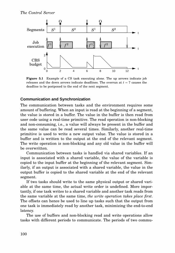
The Control Server

2

00 2 4 6 8 10 12

t

t

tSegments

Jobexecution

CBSbudget

S1 S1 S2S2

f 1f 1 f 2 f 2

II OO

Figure 5.1 Example of a CS task executing alone. The up arrows indicate jobreleases and the down arrows indicate deadlines. The overrun at t = 7 causes thedeadline to be postponed to the end of the next segment.

Communication and Synchronization

The communication between tasks and the environment requires someamount of buffering. When an input is read at the beginning of a segment,the value is stored in a buffer. The value in the buffer is then read fromuser code using a real­time primitive. The read operation is non­blockingand non­consuming, i.e., a value will always be present in the buffer andthe same value can be read several times. Similarly, another real­timeprimitive is used to write a new output value. The value is stored in abuffer and is written to the output at the end of the relevant segment.The write operation is non­blocking and any old value in the buffer willbe overwritten.Communication between tasks is handled via shared variables. If an

input is associated with a shared variable, the value of the variable iscopied to the input buffer at the beginning of the relevant segment. Sim­ilarly, if an output is associated with a shared variable, the value in theoutput buffer is copied to the shared variable at the end of the relevantsegment.If two tasks should write to the same physical output or shared vari­

able at the same time, the actual write order is undefined. More impor­tantly, if one task writes to a shared variable and another task reads fromthe same variable at the same time, the write operation takes place first.The offsets can hence be used to line up tasks such that the output fromone task is immediately read by another task, minimizing the end­to­endlatency.The use of buffers and non­blocking read and write operations allow

tasks with different periods to communicate. The periods of two commu­

100

5.3 Control and Scheduling Codesign

nicating tasks need not be harmonic, even if this makes most sense intypical applications. However, for the kernel to be able to accurately de­termine if a read and write operation really occurs simultaneously, theoffsets, periods, and segment lengths of a set of communicating tasksneed to be integer multiples of a common tick size. For this purpose, com­municating tasks are gathered into task groups. This is described furtherin the implementation section.

Scheduling Properties

From a schedulability point of view, a CS task with the CPU share Ui isequivalent to a CBS server with the bandwidth Ui. In [Abeni, 1998], it isshown that a CBS can never demand more than its reserved bandwidth.The proof is based on the processor demand approach (see Section 2.2). Bypostponing the deadline when the budget is exhausted, the loading factorof the jobs served by the CBS can never exceed Ui. The same argumentholds for the modified CBS used in the CS model. A set of CBS and CStasks is thus schedulable if and only if

∑

Ui ≤ 1. (5.1)

If the segment lengths of a CS task τ i are chosen such that

lji = C ji /Ui, (5.2)

where C ji denotes the worst­case execution time (WCET) of the code func­tion f ji , overruns will never occur (i.e., the budget will never be exhaustedbefore the end of the segment), and all latencies will be constant. For taskswith large variation in their execution time, it can sometimes be advan­tageous to assign segment lengths that are shorter than those given byEq. (5.2). This means that some deadlines will be postponed and that thetask may not always produce a new output in time, delaying the outputone or more periods. An example of when this can actually give bettercontrol performance (for a given value of Ui) is given later.

5.3 Control and Scheduling Codesign

As stated in the introductory chapter of the thesis, the control and schedul­ing codesign problem can be formulated as follows: Given a set of processesto be controlled and a computer with limited resources, a set of controllersshould be designed and scheduled as real­time tasks such that the over­all control performance is optimized. With dynamic scheduling algorithms

101

The Control Server

such as EDF and RM, the general design problem is extremely difficultdue to the complex interaction between task parameters, control param­eters, schedulability, and control performance.With our model, the link between the scheduling design and the con­

trol design is the CPU share U . Schedulability of a task set is simplydetermined by the total CPU utilization. The performance (or cost) J ofa controller executing in a real­time system can—roughly speaking—beexpressed as a function of the sampling period T , the input­output latencyLio, the sampling jitter Js, and the input­output jitter Jio:

J = J(T , Lio, Js, Jio). (5.3)

Assuming that the first segment contains the Calculate Output part ofthe control algorithm, and that the segment lengths are chosen accordingto Eq. (5.2), execution under the Control Server implies

T =∑

lk =∑

Ck/U ,

Lio = l1 = C1/U ,Js = 0,Jio = 0.

(5.4)

The only independent variable in the expressions above is U . The controlperformance can thus be expressed as a function of U only:

J = J(U). (5.5)

Assuming a linear controller, a linear plant, and a quadratic cost function,the performance of the controller for different values of U can easily becomputed using Jitterbug (see Chapter 6).The elimination of the jitter has several advantages. First, it is easy

to design a controller that compensates for a constant delay. Second, theperformance degradation associated with the jitter is removed. Third, itbecomes possible to accurately predict the performance of the controller.These properties are exploited in the codesign examples below.

Codesign Example 1: Optimal Period Selection

In this example we study the problem of optimal sampling period selectionfor a set of control loops. This type of codesign problem first appeared in[Seto et al., 1996]. A similar problem was studied in conjunction with thefeedback scheduler in Chapter 4. In those cases, however, the scheduling­induced latency and jitter was ignored.

102

5.3 Control and Scheduling Codesign

Suppose for instance that we want to control three identical integratorprocesses,

dx(t)dt

= u(t) + vc(t), (5.6)

where x is the state, u is the control signal, and vc is a continuous­timewhite noise process with zero mean and unit variance. A discrete­timecontroller is designed to minimize the continuous­time cost function

J = limT→∞

1T

∫ T

0x2(t) dt. (5.7)

assuming the sampling period h and a constant input­output latency L.As shown in Example 3.1, the cost of the optimal controller is given by

J(h, L) = 3+√3

6h+ L. (5.8)

The assumed design goal is to select sampling periods h1, h2, h3 such thata weighted sum of the cost functions,

Jtot = w1 J(h1, L1) +w2 J(h2, L2) +w3 J(h3, L3), (5.9)

is minimized subject to the utilization constraint

U = C

h1+ C

h2+ C

h3≤ 1.

Here, C is the (constant) total execution time of the control algorithm.Assigning segment lengths proportional to the parts of the algorithm, theCS model implies the same relative latency a = L/h for all controllers.Using (5.8) the objective function (5.9) can be written

Jtot =(

3+√3

6+ a

)

(w1h1 +w2h2 +w3h3).

The solution to the optimization problem is (see Eq. (4.23))

h1 = b/√w1, h2 = b/√

w2, h3 = b/√w3,

where b = C(√w1 + √w2 + √

w3). (For more general problems numericaloptimization must be performed.) Contrary to [Seto et al., 1996] (whereRM or EDF scheduling is assumed), our model allows for the latency andthe (non­existent) jitter to be accounted for in the optimization.

103

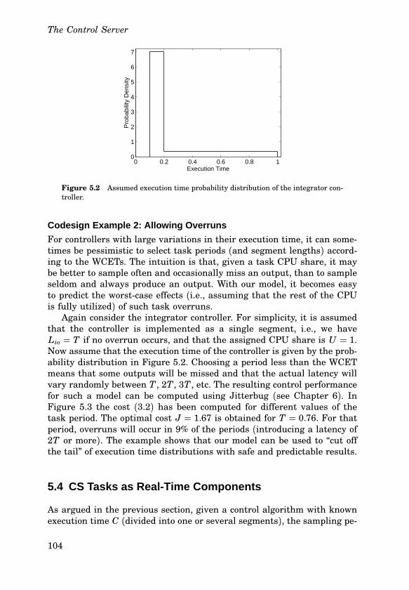
The Control Server

0 0.2 0.4 0.6 0.8 10

1

2

3

4

5

6

7

Execution Time

Pro

babi

lity

Den

sity

Figure 5.2 Assumed execution time probability distribution of the integrator con­troller.

Codesign Example 2: Allowing Overruns

For controllers with large variations in their execution time, it can some­times be pessimistic to select task periods (and segment lengths) accord­ing to the WCETs. The intuition is that, given a task CPU share, it maybe better to sample often and occasionally miss an output, than to sampleseldom and always produce an output. With our model, it becomes easyto predict the worst­case effects (i.e., assuming that the rest of the CPUis fully utilized) of such task overruns.Again consider the integrator controller. For simplicity, it is assumed

that the controller is implemented as a single segment, i.e., we haveLio = T if no overrun occurs, and that the assigned CPU share is U = 1.Now assume that the execution time of the controller is given by the prob­ability distribution in Figure 5.2. Choosing a period less than the WCETmeans that some outputs will be missed and that the actual latency willvary randomly between T , 2T , 3T , etc. The resulting control performancefor such a model can be computed using Jitterbug (see Chapter 6). InFigure 5.3 the cost (3.2) has been computed for different values of thetask period. The optimal cost J = 1.67 is obtained for T = 0.76. For thatperiod, overruns will occur in 9% of the periods (introducing a latency of2T or more). The example shows that our model can be used to “cut offthe tail” of execution time distributions with safe and predictable results.

5.4 CS Tasks as Real-Time Components

As argued in the previous section, given a control algorithm with knownexecution time C (divided into one or several segments), the sampling pe­

104

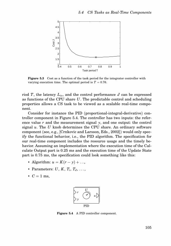
5.4 CS Tasks as Real­Time Components

0.4 0.5 0.6 0.7 0.8 0.9 11

1.5

2

2.5

3

3.5

4

4.5

5

Task period T

Cos

t J

Figure 5.3 Cost as a function of the task period for the integrator controller withvarying execution time. The optimal period is T = 0.76.

riod T , the latency Lio, and the control performance J can be expressedas functions of the CPU share U . The predictable control and schedulingproperties allows a CS task to be viewed as a scalable real­time compo­nent.Consider for instance the PID (proportional­integral­derivative) con­

troller component in Figure 5.4. The controller has two inputs: the refer­ence value r and the measurement signal y, and one output: the controlsignal u. The U knob determines the CPU share. An ordinary softwarecomponent (see, e.g., [Crnkovic and Larsson, Eds., 2002]) would only spec­ify the functional behavior, i.e., the PID algorithm. The specification forour real­time component includes the resource usage and the timely be­havior. Assuming an implementation where the execution time of the Cal­culate Output part is 0.25 ms and the execution time of the Update Statepart is 0.75 ms, the specification could look something like this:

• Algorithm: u = K (r − y) + . . .,

• Parameters: U , K , Ti, Td, . . . ,

• C = 1 ms,

r

yu

U

PID

Figure 5.4 A PID controller component.

105

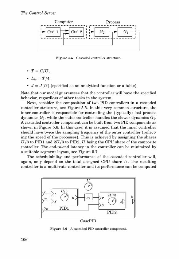
The Control Server

Ctrl 1 Ctrl 2 G2 G1

Computer Process

Figure 5.5 Cascaded controller structure.

• T = C/U ,• Lio = T/4,• J = J(U) (specified as an analytical function or a table).

Note that our model guarantees that the controller will have the specifiedbehavior, regardless of other tasks in the system.Next, consider the composition of two PID controllers in a cascaded

controller structure, see Figure 5.5. In this very common structure, theinner controller is responsible for controlling the (typically) fast processdynamics G2, while the outer controller handles the slower dynamics G1.A cascaded controller component can be built from two PID components asshown in Figure 5.6. In this case, it is assumed that the inner controllershould have twice the sampling frequency of the outer controller (reflect­ing the speed of the processes). This is achieved by assigning the sharesU/3 to PID1 and 2U/3 to PID2, U being the CPU share of the compositecontroller. The end­to­end latency in the controller can be minimized bya suitable segment layout, see Figure 5.7.The schedulability and performance of the cascaded controller will,

again, only depend on the total assigned CPU share U . The resultingcontroller is a multi­rate controller and its performance can be computed

r

rr

yy

y1

y2

u

uu

U

U/32U/3

PID1PID2

CascPID

m

Figure 5.6 A cascaded PID controller component.

106

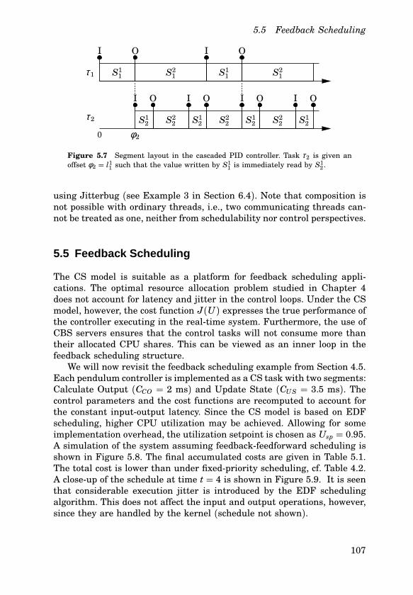
5.5 Feedback Scheduling

0

τ1

τ2

S11 S11 S21S21

S12 S12S12S12 S22S22S22

I

IIII

I

OOOO

OO

φ2

Figure 5.7 Segment layout in the cascaded PID controller. Task τ2 is given anoffset φ2 = l11 such that the value written by S11 is immediately read by S12 .

using Jitterbug (see Example 3 in Section 6.4). Note that composition isnot possible with ordinary threads, i.e., two communicating threads can­not be treated as one, neither from schedulability nor control perspectives.

5.5 Feedback Scheduling

The CS model is suitable as a platform for feedback scheduling appli­cations. The optimal resource allocation problem studied in Chapter 4does not account for latency and jitter in the control loops. Under the CSmodel, however, the cost function J(U) expresses the true performance ofthe controller executing in the real­time system. Furthermore, the use ofCBS servers ensures that the control tasks will not consume more thantheir allocated CPU shares. This can be viewed as an inner loop in thefeedback scheduling structure.We will now revisit the feedback scheduling example from Section 4.5.

Each pendulum controller is implemented as a CS task with two segments:Calculate Output (CCO = 2 ms) and Update State (CUS = 3.5 ms). Thecontrol parameters and the cost functions are recomputed to account forthe constant input­output latency. Since the CS model is based on EDFscheduling, higher CPU utilization may be achieved. Allowing for someimplementation overhead, the utilization setpoint is chosen as Usp = 0.95.A simulation of the system assuming feedback­feedforward scheduling isshown in Figure 5.8. The final accumulated costs are given in Table 5.1.The total cost is lower than under fixed­priority scheduling, cf. Table 4.2.A close­up of the schedule at time t = 4 is shown in Figure 5.9. It is seenthat considerable execution jitter is introduced by the EDF schedulingalgorithm. This does not affect the input and output operations, however,since they are handled by the kernel (schedule not shown).

107

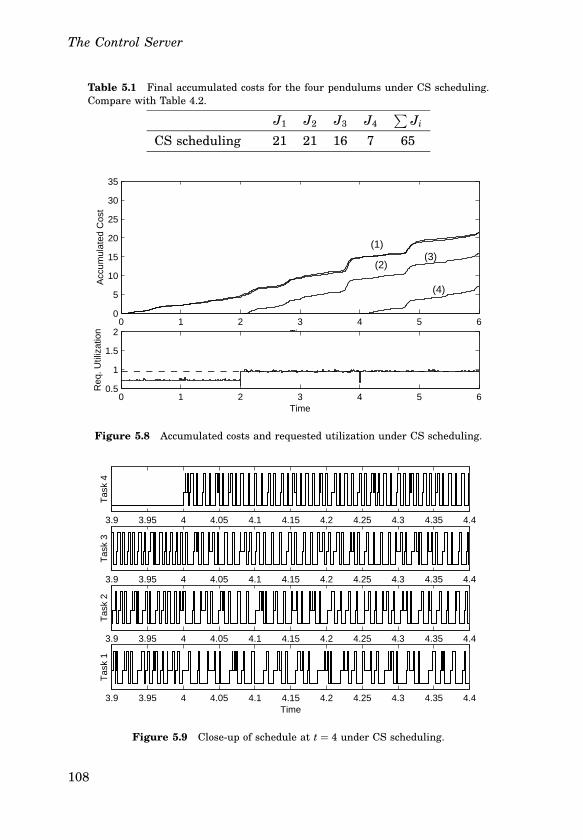
The Control Server

Table 5.1 Final accumulated costs for the four pendulums under CS scheduling.Compare with Table 4.2.

J1 J2 J3 J4∑

Ji

CS scheduling 21 21 16 7 65

0 1 2 3 4 5 60

5

10

15

20

25

30

35

Time

Acc

umul

ated

Cos

t

0 1 2 3 4 5 60.5

1

1.5

2

Req

. Util

izat

ion

Time

(1)

(2) (3)

(4)

Figure 5.8 Accumulated costs and requested utilization under CS scheduling.

3.9 3.95 4 4.05 4.1 4.15 4.2 4.25 4.3 4.35 4.4

Tas

k 1

Time

3.9 3.95 4 4.05 4.1 4.15 4.2 4.25 4.3 4.35 4.4

Tas

k 2

3.9 3.95 4 4.05 4.1 4.15 4.2 4.25 4.3 4.35 4.4

Tas

k 3

3.9 3.95 4 4.05 4.1 4.15 4.2 4.25 4.3 4.35 4.4

Tas

k 4

Figure 5.9 Close­up of schedule at t = 4 under CS scheduling.

108

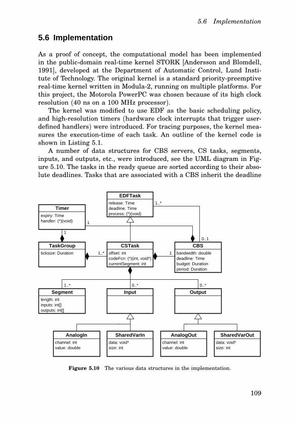
5.6 Implementation

5.6 Implementation

As a proof of concept, the computational model has been implementedin the public­domain real­time kernel STORK [Andersson and Blomdell,1991], developed at the Department of Automatic Control, Lund Insti­tute of Technology. The original kernel is a standard priority­preemptivereal­time kernel written in Modula­2, running on multiple platforms. Forthis project, the Motorola PowerPC was chosen because of its high clockresolution (40 ns on a 100 MHz processor).The kernel was modified to use EDF as the basic scheduling policy,

and high­resolution timers (hardware clock interrupts that trigger user­defined handlers) were introduced. For tracing purposes, the kernel mea­sures the execution­time of each task. An outline of the kernel code isshown in Listing 5.1.A number of data structures for CBS servers, CS tasks, segments,

inputs, and outputs, etc., were introduced, see the UML diagram in Fig­ure 5.10. The tasks in the ready queue are sorted according to their abso­lute deadlines. Tasks that are associated with a CBS inherit the deadline

CBSTaskGroup

Segment Input Output

CSTask

AnalogIn SharedVarIn AnalogOut SharedVarOut

Timer

EDFTaskrelease: Timedeadline: Timeprocess: (*)(void)expiry: Time

handler: (*)(void)

ticksize: Duration offset: intcodeFcn: (*)(int, void*)currentSegment: int

bandwidth: doubledeadline: Timebudget: Durationperiod: Duration

length: intinputs: int[]outputs: int[]

channel: intvalue: double

data: void*size: int

channel: intvalue: double

data: void*size: int

1

1

0..1

1..*

1..* 1

0..* 0..*

1..*

Figure 5.10 The various data structures in the implementation.

109

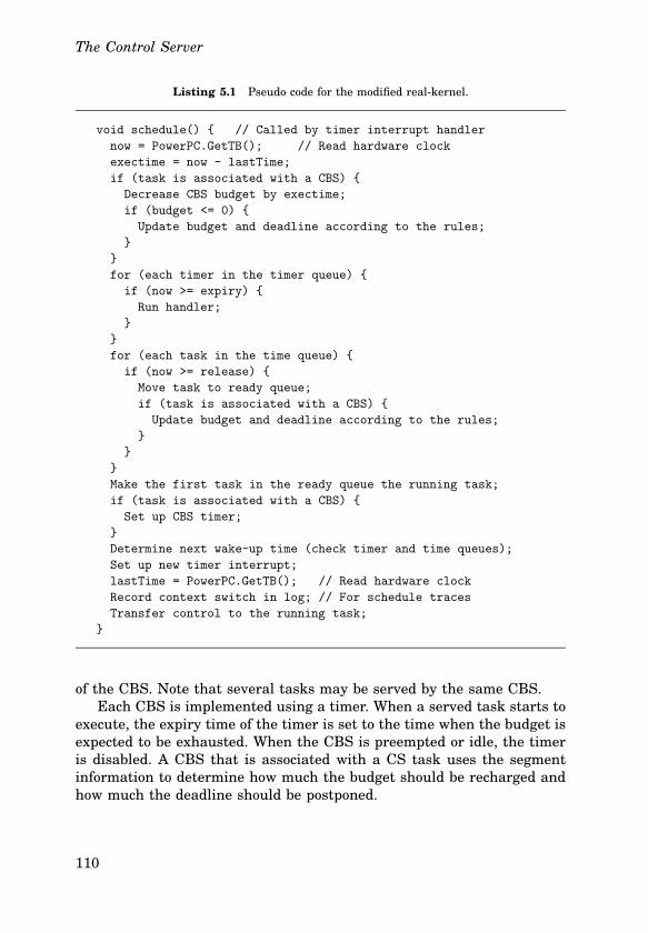
The Control Server

Listing 5.1 Pseudo code for the modified real­kernel.

void schedule() { // Called by timer interrupt handler

now = PowerPC.GetTB(); // Read hardware clock

exectime = now - lastTime;

if (task is associated with a CBS) {

Decrease CBS budget by exectime;

if (budget <= 0) {

Update budget and deadline according to the rules;

}

}

for (each timer in the timer queue) {

if (now >= expiry) {

Run handler;

}

}

for (each task in the time queue) {

if (now >= release) {

Move task to ready queue;

if (task is associated with a CBS) {

Update budget and deadline according to the rules;

}

}

}

Make the first task in the ready queue the running task;

if (task is associated with a CBS) {

Set up CBS timer;

}

Determine next wake-up time (check timer and time queues);

Set up new timer interrupt;

lastTime = PowerPC.GetTB(); // Read hardware clock

Record context switch in log; // For schedule traces

Transfer control to the running task;

}

of the CBS. Note that several tasks may be served by the same CBS.Each CBS is implemented using a timer. When a served task starts to

execute, the expiry time of the timer is set to the time when the budget isexpected to be exhausted. When the CBS is preempted or idle, the timeris disabled. A CBS that is associated with a CS task uses the segmentinformation to determine how much the budget should be recharged andhow much the deadline should be postponed.

110

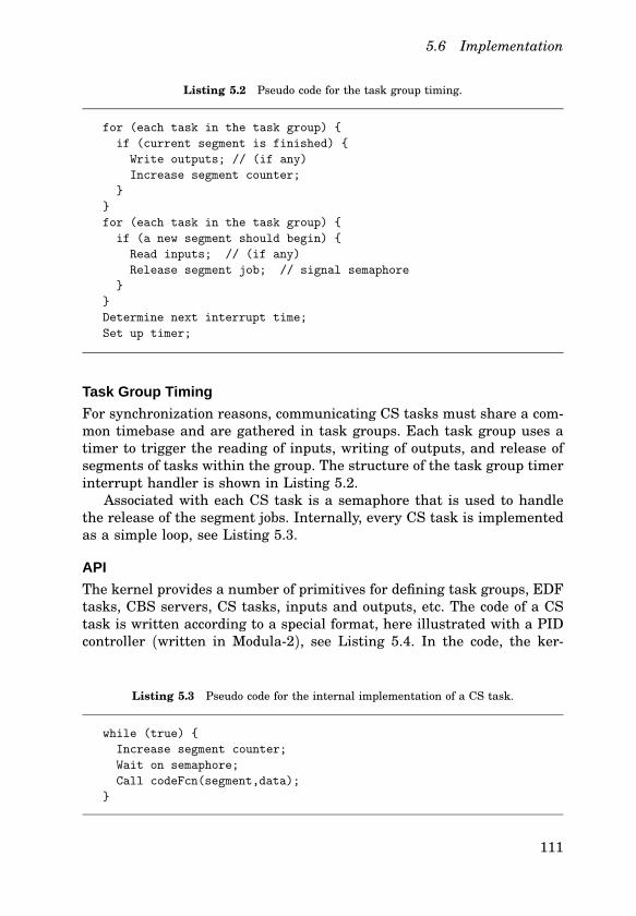
5.6 Implementation

Listing 5.2 Pseudo code for the task group timing.

for (each task in the task group) {

if (current segment is finished) {

Write outputs; // (if any)

Increase segment counter;

}

}

for (each task in the task group) {

if (a new segment should begin) {

Read inputs; // (if any)

Release segment job; // signal semaphore

}

}

Determine next interrupt time;

Set up timer;

Task Group Timing

For synchronization reasons, communicating CS tasks must share a com­mon timebase and are gathered in task groups. Each task group uses atimer to trigger the reading of inputs, writing of outputs, and release ofsegments of tasks within the group. The structure of the task group timerinterrupt handler is shown in Listing 5.2.Associated with each CS task is a semaphore that is used to handle

the release of the segment jobs. Internally, every CS task is implementedas a simple loop, see Listing 5.3.

API

The kernel provides a number of primitives for defining task groups, EDFtasks, CBS servers, CS tasks, inputs and outputs, etc. The code of a CStask is written according to a special format, here illustrated with a PIDcontroller (written in Modula­2), see Listing 5.4. In the code, the ker­

Listing 5.3 Pseudo code for the internal implementation of a CS task.

while (true) {

Increase segment counter;

Wait on semaphore;

Call codeFcn(segment,data);

}

111

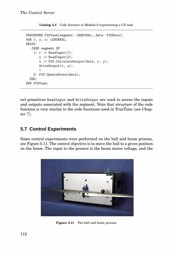
The Control Server

Listing 5.4 Code function in Modula­2 representing a CS task.

PROCEDURE PIDTask(segment: CARDINAL; data: PIDData);

VAR r, y, u: LONGREAL;

BEGIN

CASE segment OF

1: r := ReadInput(1);

y := ReadInput(2);

u := PID.CalculateOutput(data, r, y);

WriteOutput(1, u);

|

2: PID.UpdateState(data);

END;

END PIDTask;

nel primitives ReadInput and WriteOutput are used to access the inputsand outputs associated with the segment. Note that structure of the codefunction is very similar to the code functions used in TrueTime (see Chap­ter 7).

5.7 Control Experiments

Some control experiments were performed on the ball and beam process,see Figure 5.11. The control objective is to move the ball to a given positionon the beam. The input to the process is the beam motor voltage, and the

Figure 5.11 The ball and beam process.

112

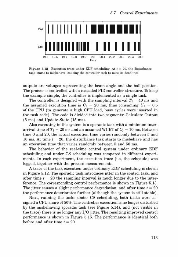
5.7 Control Experiments

19.5 19.6 19.7 19.8 19.9 20 20.1 20.2 20.3 20.4 20.5Time

Dist

Ctrl

Figure 5.12 Execution trace under EDF scheduling. At t = 20, the disturbancetask starts to misbehave, causing the controller task to miss its deadlines.

outputs are voltages representing the beam angle and the ball position.The process is controlled with a cascaded PID controller structure. To keepthe example simple, the controller is implemented as a single task.The controller is designed with the sampling interval T1 = 40 ms and

the assumed execution time is C1 = 20 ms, thus consuming U1 = 0.5of the CPU (to generate a high CPU load, busy cycles were inserted inthe task code). The code is divided into two segments: Calculate Output(5 ms) and Update State (15 ms).Also executing in the system is a sporadic task with a minimum inter­

arrival time of T2 = 20 ms and an assumed WCET of C2 = 10 ms. Betweentime 0 and 20, the actual execution time varies randomly between 5 and10 ms. At time t = 20, the disturbance task starts to misbehave and hasan execution time that varies randomly between 5 and 50 ms.The behavior of the real­time control system under ordinary EDF

scheduling and under CS scheduling was compared in different experi­ments. In each experiment, the execution trace (i.e, the schedule) waslogged, together with the process measurements.A trace of the task execution under ordinary EDF scheduling is shown

in Figure 5.12. The sporadic task introduces jitter in the control task, andafter time t = 20 the sampling interval is much longer due to the inter­ference. The corresponding control performance is shown in Figure 5.13.The jitter causes a slight performance degradation, and after time t = 20the performance deteriorates further (although the system is still stable).Next, running the tasks under CS scheduling, both tasks were as­

signed a CPU share of 50%. The controller execution is no longer disturbedby the misbehaving sporadic task (see Figure 5.14), and (not visible inthe trace) there is no longer any I/O jitter. The resulting improved controlperformance is shown in Figure 5.15. The performance is identical bothbefore and after time t = 20.

113

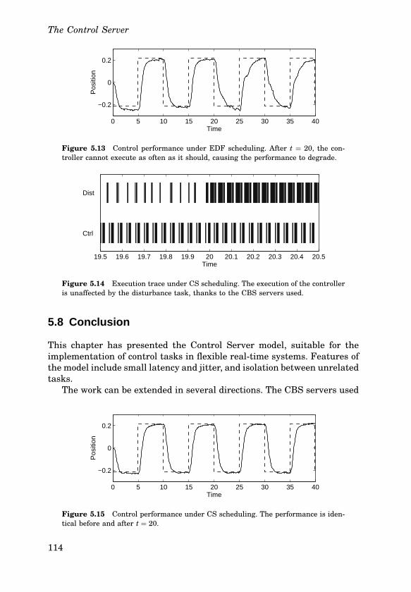
The Control Server

0 5 10 15 20 25 30 35 40

−0.2

0

0.2

Time

Pos

ition

Figure 5.13 Control performance under EDF scheduling. After t = 20, the con­troller cannot execute as often as it should, causing the performance to degrade.

19.5 19.6 19.7 19.8 19.9 20 20.1 20.2 20.3 20.4 20.5Time

Dist

Ctrl

Figure 5.14 Execution trace under CS scheduling. The execution of the controlleris unaffected by the disturbance task, thanks to the CBS servers used.

5.8 Conclusion

This chapter has presented the Control Server model, suitable for theimplementation of control tasks in flexible real­time systems. Features ofthe model include small latency and jitter, and isolation between unrelatedtasks.The work can be extended in several directions. The CBS servers used

0 5 10 15 20 25 30 35 40

−0.2

0

0.2

Time

Pos

ition

Figure 5.15 Control performance under CS scheduling. The performance is iden­tical before and after t = 20.

114

5.8 Conclusion

could be modified to use a slack stealing algorithm such as CASH [Cac­camo et al., 2000a] or GRUB [Lipari and Baruah, 2000]. This could im­prove the performance further when the system is under­utilized.We do not account for the interrupt time (including the I/O operation)

in the scheduling analysis. Possibilities for more detailed analysis arefound in [Liu and Layland, 1973] (“mixed scheduling”) and in [Jeffay andStone, 1993].

115

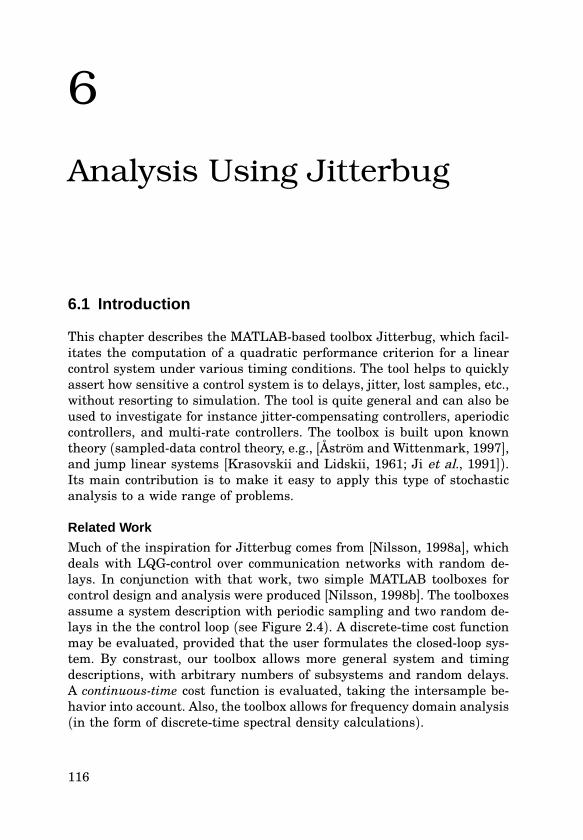
6

Analysis Using Jitterbug

6.1 Introduction

This chapter describes the MATLAB­based toolbox Jitterbug, which facil­itates the computation of a quadratic performance criterion for a linearcontrol system under various timing conditions. The tool helps to quicklyassert how sensitive a control system is to delays, jitter, lost samples, etc.,without resorting to simulation. The tool is quite general and can also beused to investigate for instance jitter­compensating controllers, aperiodiccontrollers, and multi­rate controllers. The toolbox is built upon knowntheory (sampled­data control theory, e.g., [Åström and Wittenmark, 1997],and jump linear systems [Krasovskii and Lidskii, 1961; Ji et al., 1991]).Its main contribution is to make it easy to apply this type of stochasticanalysis to a wide range of problems.

Related Work

Much of the inspiration for Jitterbug comes from [Nilsson, 1998a], whichdeals with LQG­control over communication networks with random de­lays. In conjunction with that work, two simple MATLAB toolboxes forcontrol design and analysis were produced [Nilsson, 1998b]. The toolboxesassume a system description with periodic sampling and two random de­lays in the the control loop (see Figure 2.4). A discrete­time cost functionmay be evaluated, provided that the user formulates the closed­loop sys­tem. By constrast, our toolbox allows more general system and timingdescriptions, with arbitrary numbers of subsystems and random delays.A continuous­time cost function is evaluated, taking the intersample be­havior into account. Also, the toolbox allows for frequency domain analysis(in the form of discrete­time spectral density calculations).

116

6.2 System Description

H1(z)

H1(z)

H2(z)H2(z)

H3(z)

H3(z)

G(s)yu

1

2

3

τ1

τ2

(a) (b)

Figure 6.1 A simple Jitterbug model of a computer­controlled system: (a) signalmodel and (b) timing model.

6.2 System Description

In Jitterbug, a control system is described by two parallel models: a signalmodel and a timing model. The signal model is given by a number of con­nected, linear, continuous­ and discrete­time systems. The timing modelconsists of a number of timing nodes and describes when the differentdiscrete­time systems should be updated during the control period.An example of a Jitterbug model is shown in Figure 6.1, where a

computer­controlled system is modeled by four blocks. The plant is de­scribed by the continuous­time system G, and the controller is describedby the three discrete­time systems H1, H2, and H3. The system H1 couldrepresent a periodic sampler, H2 could represent the computation of thecontrol signal, and H3 could represent the actuator. The associated tim­ing model says that, at the beginning of each period, H1 should first beexecuted (updated). Then there is a random delay τ1 until H2 is executed,and another random delay τ2 until H3 is executed. The delays could modelcomputational delays, scheduling delays, or network transmission delays.

Signal Model

The signal model consists of a number of inter­connected continuous­timeand discrete­time linear systems driven by white noise. The cost is speci­fied as a stationary, continuous­time quadratic cost function.

Continuous­Time Systems. A continuous­time system may be speci­fied in state­space form or in transfer­function form.

117

Analysis Using Jitterbug

In state­space form, the system is described by

x(t) = Ax(t) + Bu(t) + vc(t),

y0(t) = Cx(t), (continuous output)y(tk) = y0(tk) + ed(tk), (measured discrete output)

(6.1)

where vc is a continuous­time white­noise process with zero mean andcovariance1 R1c, and ed is a discrete­time white­noise process with zeromean and covariance R2d. The cost of the system is specified as

Jc = limT→∞

1T

∫ T

0

x(t)u(t)

T

Qc

x(t)u(t)

dt, (6.2)

where Qc is a positive semi­definite matrix.In transfer­function form, the system is described by

y0(t) = G(p)(

u(t) + vc(t))

, (continuous output)y(tk) = y0(tk) + ed(tk), (measured discrete output)

(6.3)

where G(p) is a strictly proper transfer function, vc is a continuous­time white­noise process with zero mean and covariance R1c, and ed isa discrete­time white­noise process with zero mean and covariance R2d.The cost of the system is specified as

Jc = limT→∞

1T

∫ T

0

y0(t)u(t)

T

Qc

y0(t)u(t)

dt, (6.4)

where Qc is a positive semi­definite matrix.Note that direct terms are not allowed (i.e., all continuous­time sys­

tems must be strictly proper). This restriction is imposed to avoid prob­lems with infinite variances and algebraic loops. Also note that there is nocontinuous­time output noise. The ability to specify discrete­time measure­ment noise in connection with the plant is only offered as a convenience.The discrete­time output noise will be translated into input noise at anyconnected discrete­time system (see Figure 6.2(c) below).

Discrete­Time Systems. A discrete­time system may be given in state­space form or in transfer­function form.

1Strictly speaking, a continuous­time white noise process has infinite variance. What wereally mean is that vc has the spectral density φ(ω ) = 1

2π R1c. See [Åström and Wittenmark,1997] for further discussion.

118

6.2 System Description

In state­space form, the system is described by

x(tk+1) = Φx(tk) + Γu(tk) + vd(tk),

y0(tk) = Cx(tk) + Du(tk), (discrete output)y(tk) = y0(tk) + ed(tk), (measured discrete output)

(6.5)

where vd and ed are discrete­time white­noise processs with zero meanand covariance

Rd = E

vd(tk)ed(tk)

vd(tk)ed(tk)

T

.

The cost of the system is specified as

Jd = limT→∞

1T

∫ T

0

x(t)y0(t)u(t)

T

Qd

x(t)y0(t)u(t)

dt, (6.6)

where Qd is a positive semi­definite matrix. Note that x(t) and y0(t) arepiecewise constant signals, while u(t) may be a continuous signal.In transfer­function form, the system is described by

y0(tk) = H(q)(

u(tk) + vd(tk))

, (discrete output)y(tk) = y0(tk) + ed(tk), (measured discrete output)

(6.7)

where H(q) is a proper transfer function, and vd and ed are discrete­timewhite­noise processs with zero mean and covariance

Rd = E

vd(tk)ed(tk)

vd(tk)ed(tk)

T

.

The cost of the system is specified as

Jd = limT→∞

1T

∫ T

0

y0(t)u(t)

T

Qd

y0(t)u(t)

dt, (6.8)

where Qd is a positive semi­definite matrix. Again, note that y0(t) is apiecewise constant signal, while u(t) may be a continuous signal.

Connecting Systems. The total system is formed by appropriatelyconnecting the inputs and outputs of a number of continuous­time anddiscrete­time systems. Throughout, multiple input­multiple output (MIMO)

119

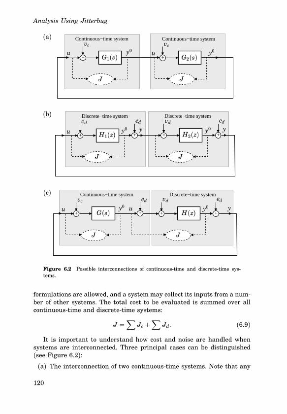
Analysis Using Jitterbug

++

Continuous−time system Continuous−time system

++ ++

Discrete−time systemDiscrete−time system

+ ++ +

Continuous−time system Discrete−time system

(a)

(b)

(c)

u

u u

u u

vc

vc vc

vd

vd vd

ed ed

ed ed

G1(s) G2(s)

H1(z) H2(z)

G(s) H(z)

J J

J J

J J

y

y y

y0y0

y0 y0

y0 y0

Figure 6.2 Possible interconnections of continuous­time and discrete­time sys­tems.

formulations are allowed, and a system may collect its inputs from a num­ber of other systems. The total cost to be evaluated is summed over allcontinuous­time and discrete­time systems:

J =∑

Jc +∑

Jd. (6.9)

It is important to understand how cost and noise are handled whensystems are interconnected. Three principal cases can be distinguished(see Figure 6.2):

(a) The interconnection of two continuous­time systems. Note that any

120

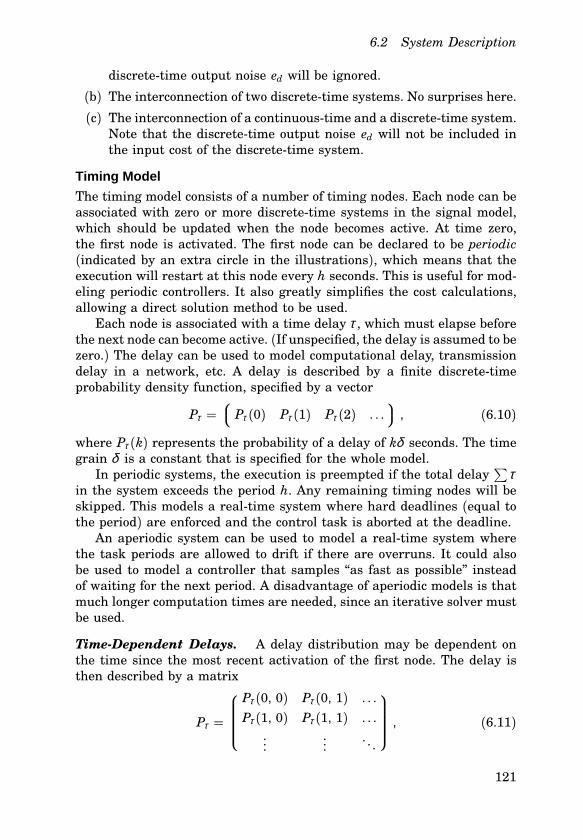
6.2 System Description

discrete­time output noise ed will be ignored.

(b) The interconnection of two discrete­time systems. No surprises here.(c) The interconnection of a continuous­time and a discrete­time system.Note that the discrete­time output noise ed will not be included inthe input cost of the discrete­time system.

Timing Model

The timing model consists of a number of timing nodes. Each node can beassociated with zero or more discrete­time systems in the signal model,which should be updated when the node becomes active. At time zero,the first node is activated. The first node can be declared to be periodic(indicated by an extra circle in the illustrations), which means that theexecution will restart at this node every h seconds. This is useful for mod­eling periodic controllers. It also greatly simplifies the cost calculations,allowing a direct solution method to be used.Each node is associated with a time delay τ , which must elapse before

the next node can become active. (If unspecified, the delay is assumed to bezero.) The delay can be used to model computational delay, transmissiondelay in a network, etc. A delay is described by a finite discrete­timeprobability density function, specified by a vector

Pτ =

Pτ (0) Pτ (1) Pτ (2) . . .

, (6.10)

where Pτ (k) represents the probability of a delay of kδ seconds. The timegrain δ is a constant that is specified for the whole model.In periodic systems, the execution is preempted if the total delay

∑

τin the system exceeds the period h. Any remaining timing nodes will beskipped. This models a real­time system where hard deadlines (equal tothe period) are enforced and the control task is aborted at the deadline.An aperiodic system can be used to model a real­time system where

the task periods are allowed to drift if there are overruns. It could alsobe used to model a controller that samples “as fast as possible” insteadof waiting for the next period. A disadvantage of aperiodic models is thatmuch longer computation times are needed, since an iterative solver mustbe used.

Time­Dependent Delays. A delay distribution may be dependent onthe time since the most recent activation of the first node. The delay isthen described by a matrix

Pτ =

Pτ (0, 0) Pτ (0, 1) . . .Pτ (1, 0) Pτ (1, 1) . . ....

.... . .

, (6.11)

121

Analysis Using Jitterbug

11

22

3

3

4

τ1τ1

τ2∑

τ < t ∑

τ ≥ t

p(2) p(3)

(a) (b)

Figure 6.3 Alternative execution paths in a Jitterbug execution model: (a) randomchoice of path and (b) choice of path depending on the time since the most recentactivation of the first node.

where Pτ ( j, k) represents the probability of a delay of kδ seconds given aprevious total delay of jδ seconds.

Node­ and Time­Dependent Update Equations. The same discrete­time system may be updated in several timing nodes. It is possible tospecify different update equations (i.e., different Φ, Γ, C and D matri­ces) in the various cases. This can be used to model a filter where theupdate equations look different depending on whether or not a measure­ment value is available. An example of this type is given later.It is also possible to make the update equations depend on the time

since the first node last became active. This can be used to model jitter­compensating controllers for example.

Random and Time­Dependent Execution Paths. For some systems,it is desirable to specify alternative execution paths (and thereby multiplenext nodes). In Jitterbug, two such cases can be modeled (see Figure 6.3):

(a) A vector n of next nodes can be specified with a probability vectorp. After the delay, execution node n(i) will be activated with proba­bility p(i). This can be used to model a sample being lost with someprobability.

(b) A vector n of next nodes can be specified with a time vector t. If thetime since the most recent activation of the first node exceeds t(i),node n(i) will be activated next. This can be used to model time­outsand various compensation schemes.

122

6.3 Internal Workings

6.3 Internal Workings

Inside Jitterbug, the states and the cost are considered in continuoustime. The inherently discrete­time states, e.g., in discrete­time controllersor filters, are treated as continuous­time states with zero dynamics. Thismeans that the total system can be written as

x(t) = Ax(t) + vc(t), (6.12)

where x collects all the states in the system, and vc is continuous­timewhite noise process with covariance Rc. To model the discrete­time changesof some states as a timing node n is activated, the state is instantaneouslytransformed by

x(t+) = Enx(t) + en(t), (6.13)where en is a discrete­time white noise process with covariance Wn.The total cost (6.9) for the system can be written as

J = limT→∞

1T

∫ T

0xT(t)Qcx(t) dt, (6.14)

where Qc is a positive semidefinite matrix.

Sampling the System

Jitterbug relies on discretized time to calculate the variance of the statesand the cost. No approximations are involved, however. Sampling thesystem (6.12) with a period of δ (the time­grain in the delay distributions)gives

x(kδ + δ ) = Φx(kδ ) + v(kδ ), (6.15)where the covariance of v is R, and the cost (6.14) becomes

J = limN→∞

1Nδ

N−1∑

k=0

(

xT (kδ )Qx(kδ ) + q)

. (6.16)

The matrices Φ, R, Q, and q are calculated as

Φ = eAδ , (6.17)

R =∫ δ

0eA(δ −τ )Rce

AT (δ −τ ) dτ , (6.18)

Q =∫ δ

0eAT tQce

At dt, (6.19)

q = tr(

Qc

∫ δ

0

∫ δ

0eA(t−τ )Rce

AT (t−τ ) dτ dt)

, (6.20)

123

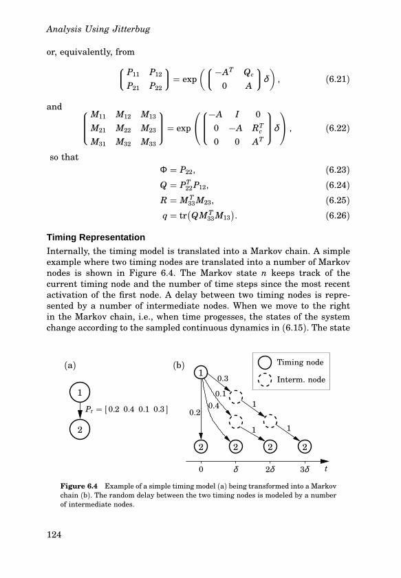
Analysis Using Jitterbug

or, equivalently, from

P11 P12

P21 P22

= exp

(

−AT Qc

0 A

δ

)

, (6.21)

and

M11 M12 M13

M21 M22 M23

M31 M32 M33

= exp

−A I 0

0 −A RTc

0 0 AT

δ

, (6.22)

so thatΦ = P22, (6.23)Q = PT22P12, (6.24)R = MT33M23, (6.25)q = tr

(

QMT33M13)

. (6.26)

Timing Representation

Internally, the timing model is translated into a Markov chain. A simpleexample where two timing nodes are translated into a number of Markovnodes is shown in Figure 6.4. The Markov state n keeps track of thecurrent timing node and the number of time steps since the most recentactivation of the first node. A delay between two timing nodes is repre­sented by a number of intermediate nodes. When we move to the rightin the Markov chain, i.e., when time progesses, the states of the systemchange according to the sampled continuous dynamics in (6.15). The state

1

1

2

2222

(a) (b)

Pτ = [ 0.2 0.4 0.1 0.3 ]

0.3

0.1

0.40.2

1

11

0 δ 2δ 3δ t

Timing node

Interm. node

Figure 6.4 Example of a simple timing model (a) being transformed into a Markovchain (b). The random delay between the two timing nodes is modeled by a numberof intermediate nodes.

124

6.3 Internal Workings

covariance P(kδ ) = E{

x(kδ )xT(kδ )}

then evolves as

P(kδ + δ ) = ΦP(kδ )ΦT + R. (6.27)

When a new timing node is visited, the states of the system change accord­ing to the discrete dynamics in (6.13). The state covariance then evolvesas

P(kδ +) = EnP(kδ )ETn +Wn, (6.28)where Wn is the covariance of the discrete­time noise en(kδ ) in node n.Combining the above, we define Φn as

Φn ={

Φ if n is an intermediate node,EnΦ if n is a timing node,

(6.29)

and similarly Rn as

Rn ={

R if n is an intermediate node,

EnRETn +Wn if n is a timing node.

(6.30)

(Note that the expressions above are not valid for the case of zero delaybetween two timing nodes—that case must be treated separately.)

Calculating Variance and Cost

Now consider all possible Markov states simultaneously. Let πn(kδ ) bethe probability of being in Markov state n at time kδ , and let Pn(kδ ) bethe covariance of the state if the system is in Markov state n at time kδ .Furthermore, let the transition matrix of the Markov chain be σ , suchthat

π (kδ + δ ) = σπ (kδ ). (6.31)The state covariance then evolves as

Pn(kδ + δ ) =∑

i

σ niπ i(kδ )(

ΦnPi(kδ )ΦTn + Rn)

, (6.32)

and the cost in time step k is given by

1δ

∑

n

πn(kδ )(

tr(

Pn(kδ )Q)

+ q)

. (6.33)

For systems without a periodic node, Eq. (6.32) must be iterated untilthe cost and variance converge. For periodic systems, the Markov state

125

Analysis Using Jitterbug

returns to the periodic timing node every h/δ time steps. Since Eq. (6.32)is affine in P, we can find the stationary covariance P1(∞) in the periodicnode by solving a linear system of n2 equations, where n is the numberof states in the total system (see [Nilsson, 1998a]). The total cost is thencalculated over the timesteps in one period. The toolbox returns the costJ = ∞ if the system is not stable (in the mean­square sense).

Calculating Spectral Densities

For periodic systems, the toolbox can compute the discrete­time spectraldensities of all outputs as observed in the periodic timing node. This can beused for frequency­domain analysis of the closed­loop system. The spectraldensity of an output y is defined as

φ y(ω ) = 12π

∞∑

k=−∞r y(k)e−ikω , (6.34)

where r y(k) is the covariance function of y. This function is computed as

r y(k) = E{

y(t)yT(t+ kh)}

= E{

Cx(t)xT(t+ kh)CT}

= E{

CΦhkhx(t)xT(t)CT}

= CΦhkhP1(∞)CT ,(6.35)

where Φ is the average transition matrix over a period, and P1(∞) isthe stationary covariance in the periodic node. The spectral density isreturned as a linear system F(z) such that φ y(ω ) = F(eiω ).

6.4 Examples

In this section, a number of examples that illustrate the use of Jitterbugare given. Note that there is no graphical user interface to Jitterbug;rather, the timing model and the signal model are defined in a scriptusing a number of MATLAB commands. Typically, the script is iteratedover a number of interesting timing parameters to produce a cost functionplot. A summary of the available commands is given in Table 6.1.

Example 1: Distributed Control System

In this example, we will study the distributed control system shown inFigure 2.4. In the control loop, the sensor, the actuator, and the controllerare distributed among different nodes in a network. The sensor node isassumed to be time­driven, whereas the controller and actuator nodes areassumed to be event­driven. At a fixed period h, the sensor samples the

126

6.4 Examples

Table 6.1 Summary of the Jitterbug commands.

Command Description

initjitterbug Initialize a new Jitterbug system.

addtimingnode Add a timing node.

addcontsys Add a continuous­time system.

adddiscsys Add a discrete­time system to a timing node.

adddiscexec Add an execution of a previously defined discrete­timesystem.

adddisctimedep Add time­dependence to a previously defined discrete­timesystem.

calcdynamics Calculate the internal dynamics of a Jitterbug system.

calccost Calculate the total cost of a Jitterbug system and, forperiodic systems, calculate the spectral densities of theoutputs.

lqgdesign Design a discrete­time LQG controller for a continuous­time plant with a constant time delay and a continuous­time cost function.

process and sends the measurement sample over the network to the con­troller node. There, the controller computes a control signal and sends itover the network to the actuator node, where it is subsequently actuated.The Jitterbug model of the system was shown in Figure 6.1. The pro­

cess to be controlled is a DC servo, described by the continuous­time sys­tem

G(s) = 1000s(s+ 1) . (6.36)

The process is driven by white continuous­time input noise. The samplerand the actuator are described by the trivial discrete­time systems

H1(z) = H3(z) = 1. (6.37)

The process is regulated by a discrete­time PD controller given by

H2(z) = K(

1+ Tdh

z− 1z

)

, (6.38)

where K = 1.5 and Td = 0.035.In the timing model, the communication delays are modeled the two

random variables τ1 (= τ sc) and τ2 (= τ ca). The input­output latency ofthe controller is thus given by Lio = τ1 +τ2. It is assumed that Lio neverexceeds h (otherwise Jitterbug would skip the remaining updates).

127

Analysis Using Jitterbug

Listing 6.1 MATLAB commands for a Jitterbug cost calculation.

G = 1000/(s*(s+1)); % Define the process

H1 = 1; % Define the sampler

H2 = -K*(1+Td/h*(z-1)/z); % Define the controller

H3 = 1; % Define the actuator

Ptau1 = [ ... ]; % Define prob. distr. 1

Ptau2 = [ ... ]; % Define prob. distr. 2

N = initjitterbug(delta,h); % Set time-grain and period

N = addtimingnode(N,1,Ptau1,2); % Define timing node 1

N = addtimingnode(N,2,Ptau2,3); % Define timing node 2

N = addtimingnode(N,3); % Define timing node 3

N = addcontsys(N,1,G,4,Q,R1,R2); % Add plant + cost and noise

N = adddiscsys(N,2,H1,1,1); % Add sampler to node 1

N = adddiscsys(N,3,H2,2,2); % Add controller to node 2

N = adddiscsys(N,4,H3,3,3); % Add actuator to node 3

N = calcdynamics(N); % Calculate internal dynamics

J = calccost(N); % Calculate the total cost

The performance of the controller is evaluted using the cost function

J = limT→∞

1T

∫ T

0

(

y2(t) + u2(t))

dt. (6.39)

An outline of the MATLAB commands needed to specify the model andcompute the value of the cost function are given in Listing 6.1.

Sampling Period and Constant Input­Ouput Latency. A controlsystem can typically give satisfactory performance over a range of sam­pling periods. In textbooks on digital control (e.g., [Åström and Witten­mark, 1997]), rules of thumb for sampling period selection are often given.One such rule suggests that the sampling interval h should be chosen suchthat 0.2 < ω bh < 0.6, whereω b is the bandwidth of the closed­loop system.In our case, a continuous­time PD controller with the given parameterswould give a bandwidth of about ω b = 80 rad/s. This would imply a sam­pling period of between 2.5 and 7.5 ms. The effect of input­output latencyis typically not considered in such rules of thumb, however. Using Jit­terbug, the combined effect of sampling period and latency can be easilyinvestigated. In Figure 6.5, the cost function (6.39) for the distributedcontrol system has been evaluated for different sampling periods in theinterval 1 to 10 milliseconds, and for constant input­output latency rang­ing from 0 to 100% of the sampling interval. As can be seen, a one­sample

128

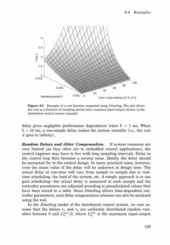
6.4 Examples

020

4060

80100

0.001

0.005

0.0101

1.5

2

2.5

3

Input−output latency (in % of h)Sampling period h

Cos

t J

Figure 6.5 Example of a cost function computed using Jitterbug. The plot showsthe cost as a function of sampling period and a constant input­output latency in thedistributed control system example.

delay gives negligible performance degradation when h = 1 ms. Whenh = 10 ms, a one­sample delay makes the system unstable (i.e., the costJ goes to infinity).

Random Delays and Jitter Compensation. If system resources arevery limited (as they often are in embedded control applications), thecontrol engineer may have to live with long sampling intervals. Delay inthe control loop then becomes a serious issue. Ideally, the delay shouldbe accounted for in the control design. In many practical cases, however,even the mean value of the delay will be unknown at design time. Theactual delay at run­time will vary from sample to sample due to real­time scheduling, the load of the system, etc. A simple approach is to usegain scheduling—the actual delay is measured in each sample and thecontroller parameters are adjusted according to precalculated values thathave been stored in a table. Since Jitterbug allows time­dependent con­troller parameters, such delay compensation schemes can also be analyzedusing the tool.In the Jitterbug model of the distributed control system, we now as­

sume that the delays τ1 and τ2 are uniformly distributed random vari­ables between 0 and Lmaxio /2, where Lmaxio is the maximum input­output

129

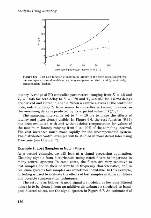
Analysis Using Jitterbug

0 20 40 60 80 1001.5

2

2.5

3

3.5

4

4.5

Maximum input−output latency (in % of h)

Cos

t J

Figure 6.6 Cost as a function of maximum latency in the distributed control sys­tem example with random delays: no delay compensation (full), and dynamic delaycompensation (dashed).

latency. A range of PD controller parameters (ranging from K = 1.5 andTd = 0.035 for zero delay to K = 0.78 and Td = 0.052 for 7.5 ms delay)are derived and stored in a table. When a sample arrives at the controllernode, only the delay τ1 from sensor to controller is known, however, sothe remaining delay is predicted by its expected value of Lmaxio /4.The sampling interval is set to h = 10 ms to make the effects of

latency and jitter clearly visible. In Figure 6.6, the cost function (6.39)has been evaluated with and without delay compensation for values ofthe maximum latency ranging from 0 to 100% of the sampling interval.The cost increases much more rapidly for the uncompensated system.The distributed control example will be studied in more detail later usingTrueTime (see Chapter 7).

Example 2: Lost Samples in Notch Filters

As a second example, we will look at a signal processing application.Cleaning signals from disturbances using notch filters is important inmany control systems. In some cases, the filters are very sensitive tolost samples due to their narrow­band frequency characteristics, and inreal­time systems lost samples are sometimes inevitable. In this example,Jitterbug is used to evaluate the effects of lost samples in different filtersand possible compensation techniques.The setup is as follows. A good signal x (modeled as low­pass filtered

noise) is to be cleaned from an additive disturbance e (modeled as band­pass filtered noise), see the signal spectra in Figure 6.7. An estimate x of

130

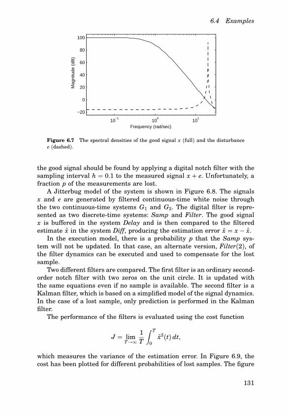
6.4 Examples

Frequency (rad/sec)

Mag

nitu

de (

dB)

10−1

100

101

−20

0

20

40

60

80

100

Figure 6.7 The spectral densities of the good signal x (full) and the disturbancee (dashed).

the good signal should be found by applying a digital notch filter with thesampling interval h = 0.1 to the measured signal x + e. Unfortunately, afraction p of the measurements are lost.A Jitterbug model of the system is shown in Figure 6.8. The signals

x and e are generated by filtered continuous­time white noise throughthe two continuous­time systems G1 and G2. The digital filter is repre­sented as two discrete­time systems: Samp and Filter. The good signalx is buffered in the system Delay and is then compared to the filteredestimate x in the system Diff, producing the estimation error x = x − x.In the execution model, there is a probability p that the Samp sys­

tem will not be updated. In that case, an alternate version, Filter(2), ofthe filter dynamics can be executed and used to compensate for the lostsample.Two different filters are compared. The first filter is an ordinary second­

order notch filter with two zeros on the unit circle. It is updated withthe same equations even if no sample is available. The second filter is aKalman filter, which is based on a simplified model of the signal dynamics.In the case of a lost sample, only prediction is performed in the Kalmanfilter.The performance of the filters is evaluated using the cost function

J = limT→∞

1T

∫ T

0x2(t) dt,

which measures the variance of the estimation error. In Figure 6.9, thecost has been plotted for different probabilities of lost samples. The figure

131

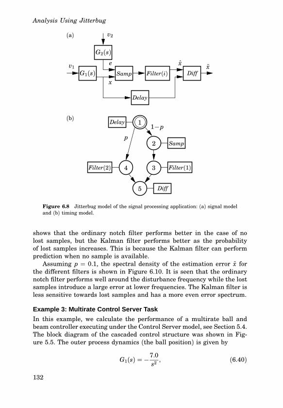
Analysis Using Jitterbug

v1

v2

e

x

xx

G1(s)

G2(s)

Samp

Samp

Diff

Diff

Delay

Delay

Filter(i)

1

2

34

5

1−pp

Filter(1)Filter(2)

(a)

(b)

Figure 6.8 Jitterbug model of the signal processing application: (a) signal modeland (b) timing model.

shows that the ordinary notch filter performs better in the case of nolost samples, but the Kalman filter performs better as the probabilityof lost samples increases. This is because the Kalman filter can performprediction when no sample is available.Assuming p = 0.1, the spectral density of the estimation error x for

the different filters is shown in Figure 6.10. It is seen that the ordinarynotch filter performs well around the disturbance frequency while the lostsamples introduce a large error at lower frequencies. The Kalman filter isless sensitive towards lost samples and has a more even error spectrum.

Example 3: Multirate Control Server Task

In this example, we calculate the performance of a multirate ball andbeam controller executing under the Control Server model, see Section 5.4.The block diagram of the cascaded control structure was shown in Fig­ure 5.5. The outer process dynamics (the ball position) is given by

G1(s) = −7.0s2

, (6.40)

132

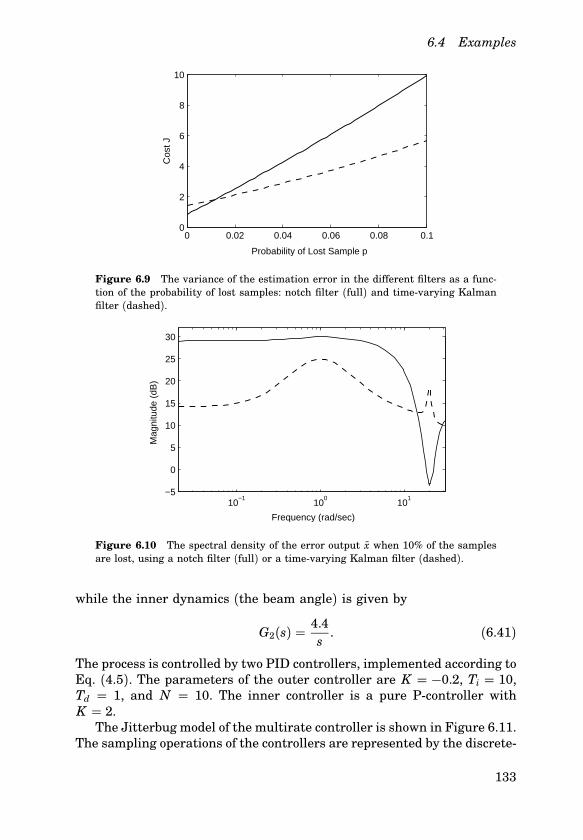
6.4 Examples

0 0.02 0.04 0.06 0.08 0.10

2

4

6

8

10

Cos

t J

Probability of Lost Sample p

Figure 6.9 The variance of the estimation error in the different filters as a func­tion of the probability of lost samples: notch filter (full) and time­varying Kalmanfilter (dashed).

Frequency (rad/sec)

Mag

nitu

de (

dB)

10−1

100

101

−5

0

5

10

15

20

25

30

Figure 6.10 The spectral density of the error output x when 10% of the samplesare lost, using a notch filter (full) or a time­varying Kalman filter (dashed).

while the inner dynamics (the beam angle) is given by

G2(s) = 4.4s

. (6.41)

The process is controlled by two PID controllers, implemented according toEq. (4.5). The parameters of the outer controller are K = −0.2, Ti = 10,Td = 1, and N = 10. The inner controller is a pure P­controller withK = 2.The Jitterbug model of the multirate controller is shown in Figure 6.11.

The sampling operations of the controllers are represented by the discrete­

133

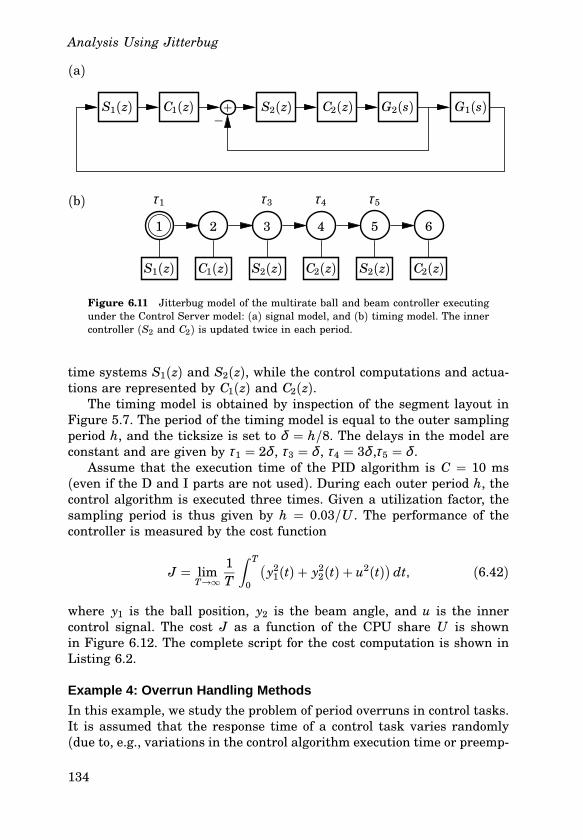
Analysis Using Jitterbug

1 2 3 4 5 6

(a)

(b)

S1(z)

S1(z)

C1(z)

C1(z)

S2(z)S2(z)

S2(z)

C2(z)C2(z)

C2(z) G2(s) G1(s)

τ1 τ3 τ4 τ5

+−

Figure 6.11 Jitterbug model of the multirate ball and beam controller executingunder the Control Server model: (a) signal model, and (b) timing model. The innercontroller (S2 and C2) is updated twice in each period.

time systems S1(z) and S2(z), while the control computations and actua­tions are represented by C1(z) and C2(z).The timing model is obtained by inspection of the segment layout in

Figure 5.7. The period of the timing model is equal to the outer samplingperiod h, and the ticksize is set to δ = h/8. The delays in the model areconstant and are given by τ1 = 2δ , τ3 = δ , τ4 = 3δ ,τ5 = δ .Assume that the execution time of the PID algorithm is C = 10 ms

(even if the D and I parts are not used). During each outer period h, thecontrol algorithm is executed three times. Given a utilization factor, thesampling period is thus given by h = 0.03/U . The performance of thecontroller is measured by the cost function

J = limT→∞

1T

∫ T

0

(

y21(t) + y22(t) + u2(t))

dt, (6.42)

where y1 is the ball position, y2 is the beam angle, and u is the innercontrol signal. The cost J as a function of the CPU share U is shownin Figure 6.12. The complete script for the cost computation is shown inListing 6.2.

Example 4: Overrun Handling Methods

In this example, we study the problem of period overruns in control tasks.It is assumed that the response time of a control task varies randomly(due to, e.g., variations in the control algorithm execution time or preemp­

134

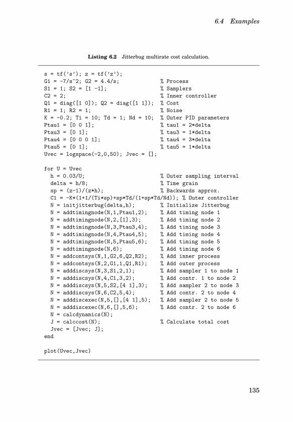
6.4 Examples

Listing 6.2 Jitterbug multirate cost calculation.

s = tf(’s’); z = tf(’z’);

G1 = -7/s^2; G2 = 4.4/s; % Process

S1 = 1; S2 = [1 -1]; % Samplers

C2 = 2; % Inner controller

Q1 = diag([1 0]); Q2 = diag([1 1]); % Cost

R1 = 1; R2 = 1; % Noise

K = -0.2; Ti = 10; Td = 1; Nd = 10; % Outer PID parameters

Ptau1 = [0 0 1]; % tau1 = 2*delta

Ptau3 = [0 1]; % tau3 = 1*delta

Ptau4 = [0 0 0 1]; % tau4 = 3*delta

Ptau5 = [0 1]; % tau5 = 1*delta

Uvec = logspace(-2,0,50); Jvec = [];

for U = Uvec

h = 0.03/U; % Outer sampling interval

delta = h/8; % Time grain

sp = (z-1)/(z*h); % Backwards approx.

C1 = -K*(1+1/(Ti*sp)+sp*Td/(1+sp*Td/Nd)); % Outer controller

N = initjitterbug(delta,h); % Initialize Jitterbug

N = addtimingnode(N,1,Ptau1,2); % Add timing node 1

N = addtimingnode(N,2,[1],3); % Add timing node 2

N = addtimingnode(N,3,Ptau3,4); % Add timing node 3

N = addtimingnode(N,4,Ptau4,5); % Add timing node 4

N = addtimingnode(N,5,Ptau5,6); % Add timing node 5

N = addtimingnode(N,6); % Add timing node 6

N = addcontsys(N,1,G2,6,Q2,R2); % Add inner process

N = addcontsys(N,2,G1,1,Q1,R1); % Add outer process

N = adddiscsys(N,3,S1,2,1); % Add sampler 1 to node 1

N = adddiscsys(N,4,C1,3,2); % Add contr. 1 to node 2

N = adddiscsys(N,5,S2,[4 1],3); % Add sampler 2 to node 3

N = adddiscsys(N,6,C2,5,4); % Add contr. 2 to node 4

N = adddiscexec(N,5,[],[4 1],5); % Add sampler 2 to node 5

N = adddiscexec(N,6,[],5,6); % Add contr. 2 to node 6

N = calcdynamics(N);

J = calccost(N); % Calculate total cost

Jvec = [Jvec; J];

end

plot(Uvec,Jvec)

135

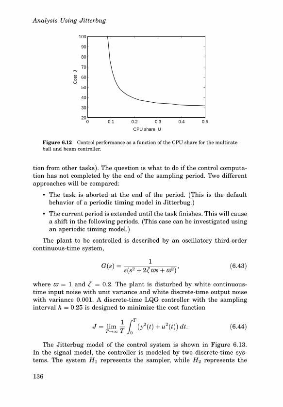
Analysis Using Jitterbug

0 0.1 0.2 0.3 0.4 0.520

30

40

50

60

70

80

90

100

CPU share U

Cos

t J

Figure 6.12 Control performance as a function of the CPU share for the multirateball and beam controller.

tion from other tasks). The question is what to do if the control computa­tion has not completed by the end of the sampling period. Two differentapproaches will be compared:

• The task is aborted at the end of the period. (This is the defaultbehavior of a periodic timing model in Jitterbug.)

• The current period is extended until the task finishes. This will causea shift in the following periods. (This case can be investigated usingan aperiodic timing model.)

The plant to be controlled is described by an oscillatory third­ordercontinuous­time system,

G(s) = 1s(s2 + 2ζ ω s+ ω 2) , (6.43)

where ω = 1 and ζ = 0.2. The plant is disturbed by white continuous­time input noise with unit variance and white discrete­time output noisewith variance 0.001. A discrete­time LQG controller with the samplinginterval h = 0.25 is designed to minimize the cost function

J = limT→∞

1T

∫ T

0

(

y2(t) + u2(t))

dt. (6.44)

The Jitterbug model of the control system is shown in Figure 6.13.In the signal model, the controller is modeled by two discrete­time sys­tems. The system H1 represents the sampler, while H2 represents the

136

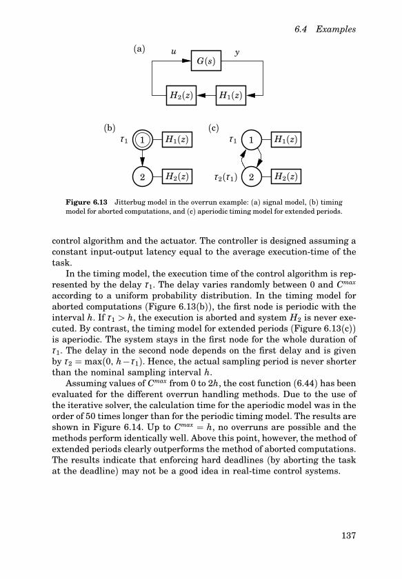
6.4 Examples

11

22

(a)

(b) (c)H1(z)

H1(z)

H1(z)

H2(z)

H2(z)

H2(z)

G(s)

τ1τ1

τ2(τ1)

u y

Figure 6.13 Jitterbug model in the overrun example: (a) signal model, (b) timingmodel for aborted computations, and (c) aperiodic timing model for extended periods.

control algorithm and the actuator. The controller is designed assuming aconstant input­output latency equal to the average execution­time of thetask.In the timing model, the execution time of the control algorithm is rep­

resented by the delay τ1. The delay varies randomly between 0 and Cmaxaccording to a uniform probability distribution. In the timing model foraborted computations (Figure 6.13(b)), the first node is periodic with theinterval h. If τ1 > h, the execution is aborted and system H2 is never exe­cuted. By contrast, the timing model for extended periods (Figure 6.13(c))is aperiodic. The system stays in the first node for the whole duration ofτ1. The delay in the second node depends on the first delay and is givenby τ2 = max(0, h−τ1). Hence, the actual sampling period is never shorterthan the nominal sampling interval h.Assuming values of Cmax from 0 to 2h, the cost function (6.44) has been

evaluated for the different overrun handling methods. Due to the use ofthe iterative solver, the calculation time for the aperiodic model was in theorder of 50 times longer than for the periodic timing model. The results areshown in Figure 6.14. Up to Cmax = h, no overruns are possible and themethods perform identically well. Above this point, however, the method ofextended periods clearly outperforms the method of aborted computations.The results indicate that enforcing hard deadlines (by aborting the taskat the deadline) may not be a good idea in real­time control systems.

137

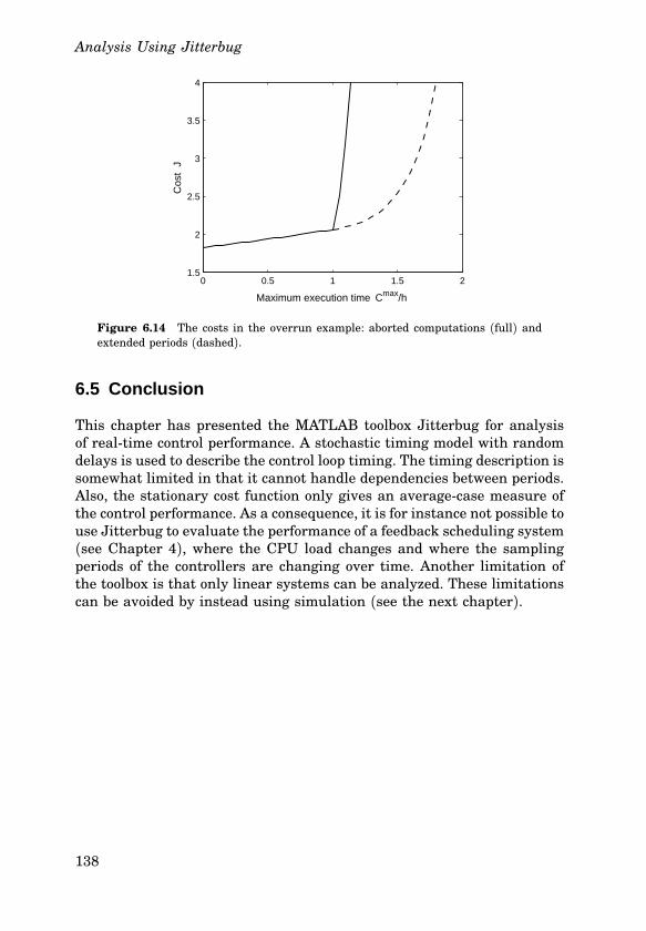
Analysis Using Jitterbug

0 0.5 1 1.5 21.5

2

2.5

3

3.5

4

Maximum execution time Cmax/h

Cos

t J

Figure 6.14 The costs in the overrun example: aborted computations (full) andextended periods (dashed).

6.5 Conclusion

This chapter has presented the MATLAB toolbox Jitterbug for analysisof real­time control performance. A stochastic timing model with randomdelays is used to describe the control loop timing. The timing description issomewhat limited in that it cannot handle dependencies between periods.Also, the stationary cost function only gives an average­case measure ofthe control performance. As a consequence, it is for instance not possible touse Jitterbug to evaluate the performance of a feedback scheduling system(see Chapter 4), where the CPU load changes and where the samplingperiods of the controllers are changing over time. Another limitation ofthe toolbox is that only linear systems can be analyzed. These limitationscan be avoided by instead using simulation (see the next chapter).

138

7

Simulation Using TrueTime

7.1 Introduction

The use of Jitterbug assumes knowledge of sampling period and latencydistributions. This information can be difficult to obtain without access tomeasurements from the true target system under implementation. Also,the analysis cannot capture all the details and nonlinearities (especiallyin the real­time scheduling) of the computer system. A natural approachis to use simulation instead. However, today’s simulation tools make itdifficult to simulate the true temporal behavior of control loops. Whatis normally done is to introduce time delays in the control loop repre­senting average­case or worst­case delays. Taking a different approach,the MATLAB/Simulink­based tool TrueTime facilitates simulation of thetemporal behavior of a multitasking real­time kernel executing controllertasks. The tasks are controlling processes that are modeled as ordinarySimulink blocks. TrueTime also makes it possible to simulate simple mod­els of communication networks and their influence on networked controlloops. Different scheduling policies may be used (e.g., fixed­priority orearliest­deadline­first scheduling).Furthermore, TrueTime can be used as an experimental platform for

research on dynamic real­time control systems. For instance, it is possibleto study compensation schemes that adjust the control algorithm basedon measurements of actual timing variations. It is also easy to experimentwith more flexible approaches to real­time scheduling of controllers, suchas feedback scheduling (see Chapter 4).In TrueTime, computer and network blocks are introduced. The com­

puter blocks are event­driven and execute user­defined tasks and inter­rupt handlers representing, e.g., I/O tasks, control algorithms, and net­work interfaces. The scheduling policy of the individual computer blocks

139

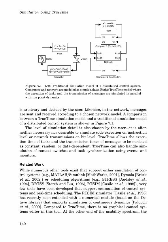
Simulation Using TrueTime

DelayDelay

x’ = Ax+Bu y = Cx+Du

Plant

y(n)=Cx(n)+Du(n)x(n+1)=Ax(n)+Bu(n)

Controller

x’ = Ax+Bu y = Cx+Du

Plant

Snd1

Snd2

Rcv1

Rcv2

Network

RcvSnd

Computer 2 (Controller)

A/D

Rcv

D/A

Snd

Computer 1 (Remote I/O)

Figure 7.1 Left: Traditional simulation model of a distributed control system.Computers and network are modeled as simple delays. Right: TrueTime model wherethe execution of tasks and the transmission of messages are simulated in parallelwith the plant dynamics.

is arbitrary and decided by the user. Likewise, in the network, messagesare sent and received according to a chosen network model. A comparisonbetween a TrueTime simulation model and a traditional simulation modelof a distributed control system is shown in Figure 7.1.The level of simulation detail is also chosen by the user—it is often

neither necessary nor desirable to simulate code execution on instructionlevel or network transmissions on bit level. TrueTime allows the execu­tion time of tasks and the transmission times of messages to be modeledas constant, random, or data­dependent. TrueTime can also handle sim­ulation of context switches and task synchronization using events andmonitors.

Related Work

While numerous other tools exist that support either simulation of con­trol systems (e.g., MATLAB/Simulink [MathWorks, 2001], Dymola [Brücket al., 2002]) or scheduling algorithms (e.g., STRESS [Audsley et al.,1994], DRTSS [Storch and Liu, 1996], RTSIM [Casile et al., 1998]), veryfew tools have been developed that support cosimulation of control sys­tems and real­time scheduling. The RTSIM simulator [Casile et al., 1998]has recently been extended with a numerical module (based on the Oc­tave library) that supports simulation of continuous dynamics [Palopoliet al., 2000]. Compared to TrueTime, there is no graphical control sys­tems editor in this tool. At the other end of the usability spectrum, the

140

7.2 Overview

simulation tool presented in [El­khoury and Törngren, 2001] is entirelybased on graphical modeling in Simulink, but is limited to predefined net­work and CPU scheduling policies (currently, CAN networks and fixed­priority scheduling). Ptolemy [Bhattacharyya et al., 2002] is a tool formodeling and simulation of heterogeneous (multi­domain) systems, suchas mixed continuous­time/discrete­event systems. The recently developedtimed multitasking (TM) domain [Liu and Lee, 2003] adds the possibilityto model fixed­priority scheduling of tasks with fixed execution times.An early, tick­based prototype of the TrueTime simulator was pre­

sented in [Eker and Cervin, 1999]. The current version is event­basedand written in C++, reducing simulation times by an order of magnitudeor more. Furthermore, the new version supports simulation of external in­terrupts, context switches, and several network medium access protocols.It also adds the possibility to model control tasks using ordinary Simulinkblock diagrams.

7.2 Overview

The TrueTime block library is shown in Figure 7.2. Two blocks are avail­able: the TrueTime Kernel block and the TrueTime Network block. Bothblocks are event­driven, with the execution determined both by internaland external events. Internal events are time­related and correspond toevents such as “a timer has expired,” “a task has finished its execution,” or“a message has completed its transmission.” External events correspondto external interrupts, such as “a message arrived on the network” or “theengine crank angle passed zero degrees.”The block inputs are assumed to be discrete­time signals, except the

signals connected to the A/D converters of the computer block, whichmay be continuous­time signals. All outputs are discrete­time signals. TheSchedule and Monitors outputs display the allocation of common resources(CPU, monitors, network) during the simulation.The blocks are implemented as variable­step, discrete­time Simulink

S­functions and are written in C++. The Simulink engine is only used fortiming and for interfacing with the rest of the model (i.e., the continuousdynamics). It should thus be easy to port the blocks to other simulationenvironments, provided that these environments support event detection(zero­crossing detection).

141

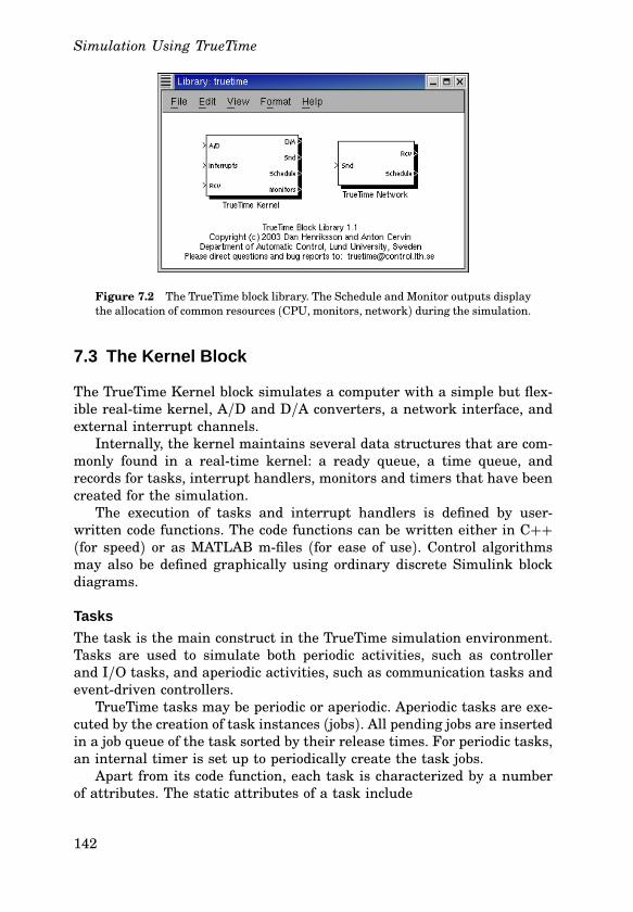
Simulation Using TrueTime

Figure 7.2 The TrueTime block library. The Schedule and Monitor outputs displaythe allocation of common resources (CPU, monitors, network) during the simulation.

7.3 The Kernel Block

The TrueTime Kernel block simulates a computer with a simple but flex­ible real­time kernel, A/D and D/A converters, a network interface, andexternal interrupt channels.Internally, the kernel maintains several data structures that are com­

monly found in a real­time kernel: a ready queue, a time queue, andrecords for tasks, interrupt handlers, monitors and timers that have beencreated for the simulation.The execution of tasks and interrupt handlers is defined by user­

written code functions. The code functions can be written either in C++(for speed) or as MATLAB m­files (for ease of use). Control algorithmsmay also be defined graphically using ordinary discrete Simulink blockdiagrams.

Tasks

The task is the main construct in the TrueTime simulation environment.Tasks are used to simulate both periodic activities, such as controllerand I/O tasks, and aperiodic activities, such as communication tasks andevent­driven controllers.TrueTime tasks may be periodic or aperiodic. Aperiodic tasks are exe­

cuted by the creation of task instances (jobs). All pending jobs are insertedin a job queue of the task sorted by their release times. For periodic tasks,an internal timer is set up to periodically create the task jobs.Apart from its code function, each task is characterized by a number

of attributes. The static attributes of a task include

142

7.3 The Kernel Block

• a relative deadline,

• a priority,

• a worst­case execution time, and

• a period (if the task is periodic).These attributes are kept constant throughout the simulation, unless ex­plicitly changed by the user. Note that the worst­case execution time doesnot determine the actual execution time of the task (see the Code sectionbelow).In addition to these attributes, each task instance has a number of

dynamic attributes. The attributes are updated by the kernel as the sim­ulation progresses. They include

• an absolute deadline,

• a release time, and

• an execution­time budget (by default equal to the worst­case execu­tion time at the release of the job).

These attributes may also be changed by the user during simulation. De­pending on the scheduling policy, the change of an attribute may leadto a context switch. For instance, under EDF scheduling, changing theabsolute deadline of a task will result in a re­sorting of the ready queue.

Interrupts and Interrupt Handlers

Interrupts may be generated in two ways: externally or internally. An ex­ternal interrupt is associated with one of the external interrupt channelsof the computer block. The interrupt is triggered when the signal of thecorresponding channel changes value. This type of interrupt may be usedto simulate combustion engine controllers that are sampled against thecrank rotation or distributed controllers that execute when measurementsarrive from the network.Internal interrupts are associated with timers. Both periodic timers

and one­shot timers can be created. The corresponding interrupt is trig­gered when the timer expires. Timers are also used internally by thekernel to implement overrun handlers (see below).When an external or internal interrupt occurs, a user­defined inter­

rupt handler is scheduled to serve the interrupt. An interrupt handlerworks much the same way as a task, but is scheduled on a higher pri­ority level. Interrupt handlers will normally perform small, less time­consuming tasks, such as generating an event or triggering the executionof a task. An interrupt handler is defined by a name, a priority, and acode function. External interrupts also have a latency during which theyare insensitive to new invocations.

143

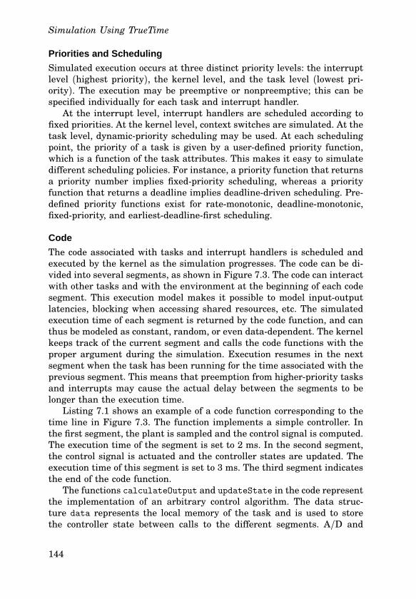
Simulation Using TrueTime

Priorities and Scheduling

Simulated execution occurs at three distinct priority levels: the interruptlevel (highest priority), the kernel level, and the task level (lowest pri­ority). The execution may be preemptive or nonpreemptive; this can bespecified individually for each task and interrupt handler.At the interrupt level, interrupt handlers are scheduled according to

fixed priorities. At the kernel level, context switches are simulated. At thetask level, dynamic­priority scheduling may be used. At each schedulingpoint, the priority of a task is given by a user­defined priority function,which is a function of the task attributes. This makes it easy to simulatedifferent scheduling policies. For instance, a priority function that returnsa priority number implies fixed­priority scheduling, whereas a priorityfunction that returns a deadline implies deadline­driven scheduling. Pre­defined priority functions exist for rate­monotonic, deadline­monotonic,fixed­priority, and earliest­deadline­first scheduling.

Code

The code associated with tasks and interrupt handlers is scheduled andexecuted by the kernel as the simulation progresses. The code can be di­vided into several segments, as shown in Figure 7.3. The code can interactwith other tasks and with the environment at the beginning of each codesegment. This execution model makes it possible to model input­outputlatencies, blocking when accessing shared resources, etc. The simulatedexecution time of each segment is returned by the code function, and canthus be modeled as constant, random, or even data­dependent. The kernelkeeps track of the current segment and calls the code functions with theproper argument during the simulation. Execution resumes in the nextsegment when the task has been running for the time associated with theprevious segment. This means that preemption from higher­priority tasksand interrupts may cause the actual delay between the segments to belonger than the execution time.Listing 7.1 shows an example of a code function corresponding to the

time line in Figure 7.3. The function implements a simple controller. Inthe first segment, the plant is sampled and the control signal is computed.The execution time of the segment is set to 2 ms. In the second segment,the control signal is actuated and the controller states are updated. Theexecution time of this segment is set to 3 ms. The third segment indicatesthe end of the code function.The functions calculateOutput and updateState in the code represent

the implementation of an arbitrary control algorithm. The data struc­ture data represents the local memory of the task and is used to storethe controller state between calls to the different segments. A/D and

144

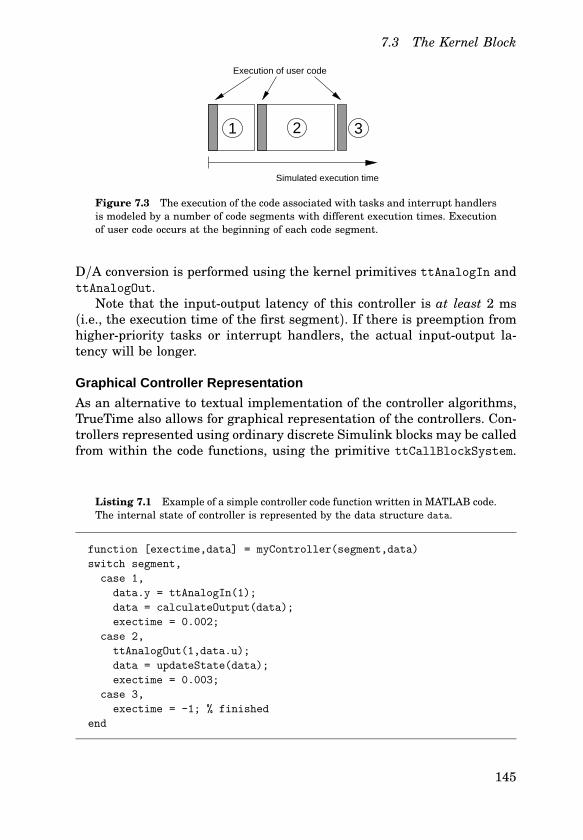
7.3 The Kernel Block

1 2 3

Simulated execution time

Execution of user code

Figure 7.3 The execution of the code associated with tasks and interrupt handlersis modeled by a number of code segments with different execution times. Executionof user code occurs at the beginning of each code segment.

D/A conversion is performed using the kernel primitives ttAnalogIn andttAnalogOut.Note that the input­output latency of this controller is at least 2 ms

(i.e., the execution time of the first segment). If there is preemption fromhigher­priority tasks or interrupt handlers, the actual input­output la­tency will be longer.

Graphical Controller Representation

As an alternative to textual implementation of the controller algorithms,TrueTime also allows for graphical representation of the controllers. Con­trollers represented using ordinary discrete Simulink blocks may be calledfrom within the code functions, using the primitive ttCallBlockSystem.

Listing 7.1 Example of a simple controller code function written in MATLAB code.The internal state of controller is represented by the data structure data.

function [exectime,data] = myController(segment,data)

switch segment,

case 1,

data.y = ttAnalogIn(1);

data = calculateOutput(data);

exectime = 0.002;

case 2,

ttAnalogOut(1,data.u);

data = updateState(data);

exectime = 0.003;

case 3,

exectime = -1; % finished

end

145

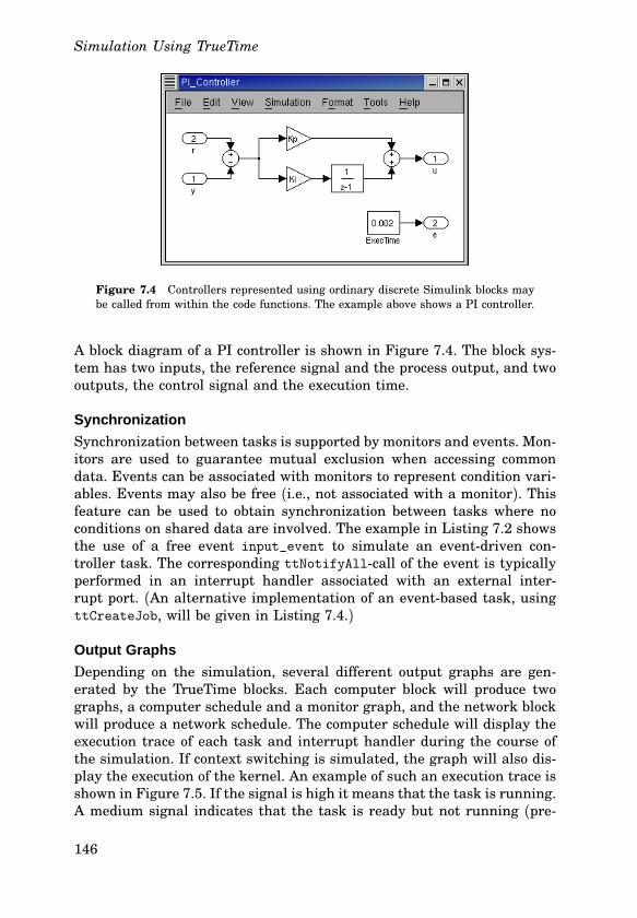
Simulation Using TrueTime

Figure 7.4 Controllers represented using ordinary discrete Simulink blocks maybe called from within the code functions. The example above shows a PI controller.

A block diagram of a PI controller is shown in Figure 7.4. The block sys­tem has two inputs, the reference signal and the process output, and twooutputs, the control signal and the execution time.

Synchronization

Synchronization between tasks is supported by monitors and events. Mon­itors are used to guarantee mutual exclusion when accessing commondata. Events can be associated with monitors to represent condition vari­ables. Events may also be free (i.e., not associated with a monitor). Thisfeature can be used to obtain synchronization between tasks where noconditions on shared data are involved. The example in Listing 7.2 showsthe use of a free event input_event to simulate an event­driven con­troller task. The corresponding ttNotifyAll­call of the event is typicallyperformed in an interrupt handler associated with an external inter­rupt port. (An alternative implementation of an event­based task, usingttCreateJob, will be given in Listing 7.4.)

Output Graphs

Depending on the simulation, several different output graphs are gen­erated by the TrueTime blocks. Each computer block will produce twographs, a computer schedule and a monitor graph, and the network blockwill produce a network schedule. The computer schedule will display theexecution trace of each task and interrupt handler during the course ofthe simulation. If context switching is simulated, the graph will also dis­play the execution of the kernel. An example of such an execution trace isshown in Figure 7.5. If the signal is high it means that the task is running.A medium signal indicates that the task is ready but not running (pre­

146

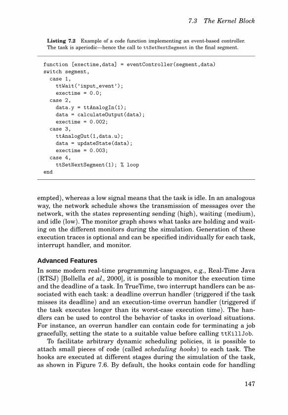
7.3 The Kernel Block

Listing 7.2 Example of a code function implementing an event­based controller.The task is aperiodic—hence the call to ttSetNextSegment in the final segment.

function [exectime,data] = eventController(segment,data)

switch segment,

case 1,

ttWait(’input_event’);

exectime = 0.0;

case 2,

data.y = ttAnalogIn(1);

data = calculateOutput(data);

exectime = 0.002;

case 3,

ttAnalogOut(1,data.u);

data = updateState(data);

exectime = 0.003;

case 4,

ttSetNextSegment(1); % loop

end

empted), whereas a low signal means that the task is idle. In an analogousway, the network schedule shows the transmission of messages over thenetwork, with the states representing sending (high), waiting (medium),and idle (low). The monitor graph shows what tasks are holding and wait­ing on the different monitors during the simulation. Generation of theseexecution traces is optional and can be specified individually for each task,interrupt handler, and monitor.

Advanced Features

In some modern real­time programming languages, e.g., Real­Time Java(RTSJ) [Bollella et al., 2000], it is possible to monitor the execution timeand the deadline of a task. In TrueTime, two interrupt handlers can be as­sociated with each task: a deadline overrun handler (triggered if the taskmisses its deadline) and an execution­time overrun handler (triggered ifthe task executes longer than its worst­case execution time). The han­dlers can be used to control the behavior of tasks in overload situations.For instance, an overrun handler can contain code for terminating a jobgracefully, setting the state to a suitable value before calling ttKillJob.To facilitate arbitrary dynamic scheduling policies, it is possible to

attach small pieces of code (called scheduling hooks) to each task. Thehooks are executed at different stages during the simulation of the task,as shown in Figure 7.6. By default, the hooks contain code for handling

147

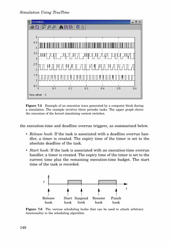
Simulation Using TrueTime

Figure 7.5 Example of an execution trace generated by a computer block duringa simulation. The example involves three periodic tasks. The upper graph showsthe execution of the kernel simulating context switches.

the execution­time and deadline overrun triggers, as summarized below.

• Release hook: If the task is associated with a deadline overrun han­dler, a timer is created. The expiry time of the timer is set to theabsolute deadline of the task.

• Start hook: If the task is associated with an execution­time overrunhandler, a timer is created. The expiry time of the timer is set to thecurrent time plus the remaining execution­time budget. The starttime of the task is recorded.

τ

t

Releasehook

Starthook

Suspendhook

Resumehook

Finishhook

Figure 7.6 The various scheduling hooks that can be used to attach arbitraryfunctionality to the scheduling algorithm.

148

7.4 The Network Block

• Suspend hook: The execution­time budget is decreased based on thetime since the last start of the task. The execution­time overruntimer is removed.

• Resume hook: The execution­time overrun timer is created again.The new start time is recorded.

• Finish hook: The execution­time budget is updated. Both overruntimers are removed.

Internal Workings

The TrueTime real­time kernel is implemented in a function runKernel

that is called by the Simulink S­function callback functions at appropriatetimes during the simulation. The workings of the kernel are describedby the pseudo code in Listing 7.3. Note that interrupt handlers are nottreated in the pseudo code; they are handled in essentially the same wayas the tasks.

Command Summary

To give an overview of the functionality of TrueTime, a summary of theavailable functions and commands is given in Table 7.1. The table is di­vided into three sections. The first section contains commands that aretypically used in the initialization script of a simulation. The second sec­tion contains commands for setting and getting task (or job) attributes.Finally, the third section contains real­time primitives that may be usedin the task code.

7.4 The Network Block

The network model is similar to the real­time kernel model, albeit simpler.The network block is event­driven and executes when messages enter orleave the network. A message contains information about the sending andthe receiving computer node, arbitrary user data (typically measurementsignals or control signals), the length of the message, and optional real­time attributes such as a priority or a deadline.In the network block, it is possible to specify the transmission rate,

the medium access control protocol (CSMA/CD, CSMA/CA, round robin,FDMA, or TDMA), and a number of other parameters. A long messagecan be split into frames that are transmitted in sequence, each with anadditional overhead. When the simulated transmission of a message hascompleted, it is put in a buffer at the receiving computer node, which isnotified by a hardware interrupt. More details on the network block canbe found in [Henriksson and Cervin, 2003].

149

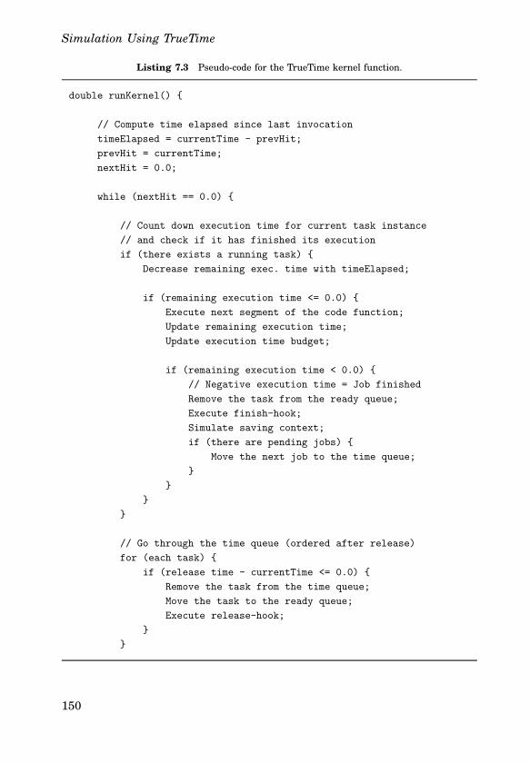
Simulation Using TrueTime

Listing 7.3 Pseudo­code for the TrueTime kernel function.

double runKernel() {

// Compute time elapsed since last invocation

timeElapsed = currentTime - prevHit;

prevHit = currentTime;

nextHit = 0.0;

while (nextHit == 0.0) {

// Count down execution time for current task instance

// and check if it has finished its execution

if (there exists a running task) {

Decrease remaining exec. time with timeElapsed;

if (remaining execution time <= 0.0) {

Execute next segment of the code function;

Update remaining execution time;

Update execution time budget;

if (remaining execution time < 0.0) {

// Negative execution time = Job finished

Remove the task from the ready queue;

Execute finish-hook;

Simulate saving context;

if (there are pending jobs) {

Move the next job to the time queue;

}

}

}

}

// Go through the time queue (ordered after release)

for (each task) {

if (release time - currentTime <= 0.0) {

Remove the task from the time queue;

Move the task to the ready queue;

Execute release-hook;

}

}

150

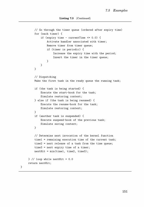
7.5 Examples

Listing 7.3 (Continued)

// Go through the timer queue (ordered after expiry time)

for (each timer) {

if (expiry time - currentTime <= 0.0) {

Activate handler associated with timer;

Remove timer from timer queue;

if (timer is periodic) {

Increase the expiry time with the period;

Insert the timer in the timer queue;

}

}

}

// Dispatching

Make the first task in the ready queue the running task;

if (the task is being started) {

Execute the start-hook for the task;

Simulate restoring context;

} else if (the task is being resumed) {

Execute the resume-hook for the task;

Simulate restoring context;

}

if (another task is suspended) {

Execute suspend-hook of the previous task;

Simulate saving context;

}

// Determine next invocation of the kernel function

time1 = remaining execution time of the current task;

time2 = next release of a task from the time queue;

time3 = next expiry time of a timer;

nextHit = min(time1, time2, time3);

} // loop while nextHit = 0.0

return nextHit;

}

151

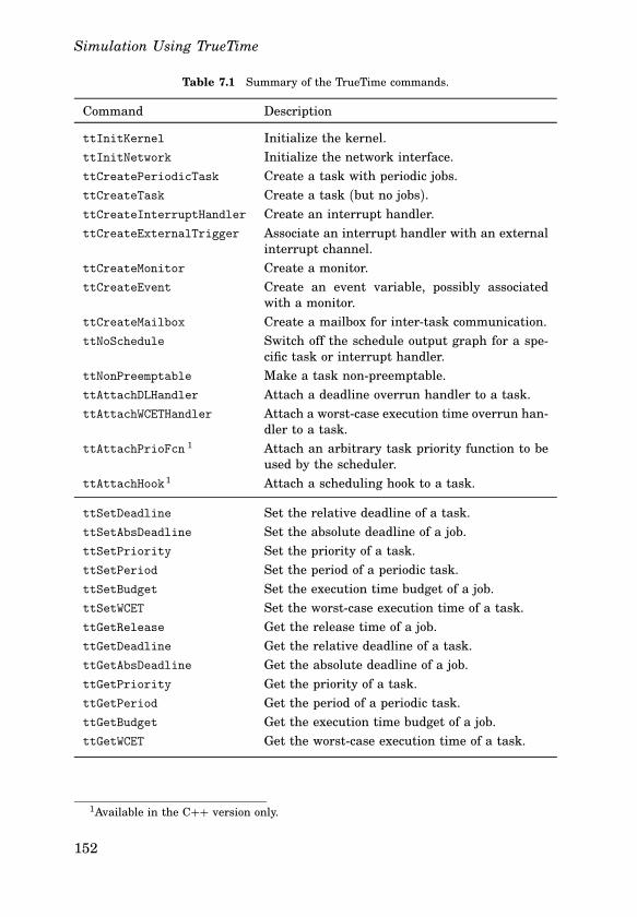
Simulation Using TrueTime

Table 7.1 Summary of the TrueTime commands.

Command Description

ttInitKernel Initialize the kernel.

ttInitNetwork Initialize the network interface.

ttCreatePeriodicTask Create a task with periodic jobs.

ttCreateTask Create a task (but no jobs).ttCreateInterruptHandler Create an interrupt handler.

ttCreateExternalTrigger Associate an interrupt handler with an externalinterrupt channel.

ttCreateMonitor Create a monitor.

ttCreateEvent Create an event variable, possibly associatedwith a monitor.

ttCreateMailbox Create a mailbox for inter­task communication.

ttNoSchedule Switch off the schedule output graph for a spe­cific task or interrupt handler.

ttNonPreemptable Make a task non­preemptable.

ttAttachDLHandler Attach a deadline overrun handler to a task.

ttAttachWCETHandler Attach a worst­case execution time overrun han­dler to a task.

ttAttachPrioFcn 1 Attach an arbitrary task priority function to beused by the scheduler.

ttAttachHook 1 Attach a scheduling hook to a task.

ttSetDeadline Set the relative deadline of a task.

ttSetAbsDeadline Set the absolute deadline of a job.

ttSetPriority Set the priority of a task.

ttSetPeriod Set the period of a periodic task.

ttSetBudget Set the execution time budget of a job.

ttSetWCET Set the worst­case execution time of a task.

ttGetRelease Get the release time of a job.

ttGetDeadline Get the relative deadline of a task.

ttGetAbsDeadline Get the absolute deadline of a job.

ttGetPriority Get the priority of a task.

ttGetPeriod Get the period of a periodic task.

ttGetBudget Get the execution time budget of a job.

ttGetWCET Get the worst­case execution time of a task.

1Available in the C++ version only.

152

7.5 Examples

Table 7.1 (Continued)

Command Description

ttCreateJob Create a job with a given release time.

ttKillJob Kill the running job of a task.

ttEnterMonitor Attempt to enter a monitor.

ttExitMonitor Exit a monitor.

ttWait Wait for an event.

ttNotifyAll Notify all tasks waiting for an event.

ttTryFetch Fetch a message from a mailbox.

ttTryPost Post a message to a mailbox.

ttCreateTimer Create a one­shot timer and associate an inter­rupt handler with the timer.

ttCreatePeriodicTimer Create a periodic timer and associate an inter­rupt handler with the timer.

ttRemoveTimer Remove a specific timer.

ttCurrentTime Get the current time in the simulation.

ttSleepUntil Put a task to sleep until a certain point in time.

ttSleep Put a task to sleep for a certain duration.

ttAnalogIn Read the value of an analog input.

ttAnalogOut Write a value to an analog output.

ttSetNextSegment Set the next segment to be executed in the codefunction.

ttInvokingTask Get the name of the task that invoked an inter­rupt handler.

ttCallBlockSystem Call a Simulink block diagram from within acode function.

ttSendMsg Send a message over the network.

ttGetMsg Get a message that has been received over thenetwork.

7.5 Examples

In this section, a number of examples that illustrate the use of TrueTimeare given.

Example 1: Distributed Control System

As a first example of simulation in TrueTime, we again turn our atten­tion to the networked control system (see Example 1 in Section 6.4). Us­ing TrueTime, detailed simulation of the distributed control system is

153

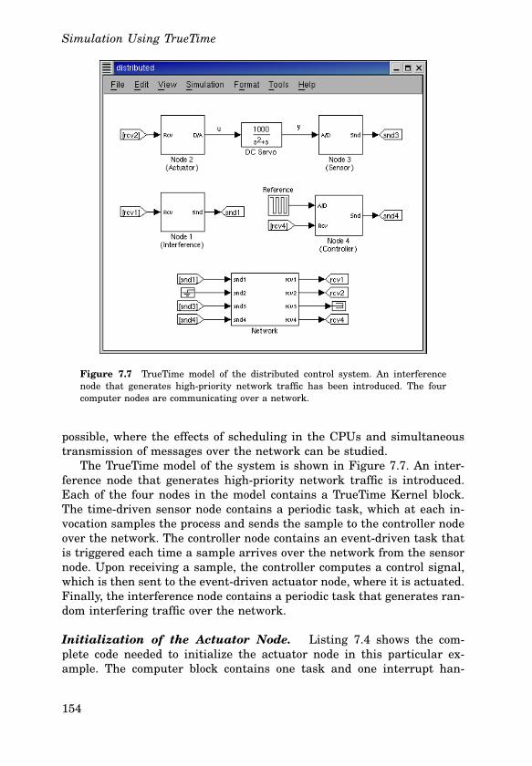
Simulation Using TrueTime

Figure 7.7 TrueTime model of the distributed control system. An interferencenode that generates high­priority network traffic has been introduced. The fourcomputer nodes are communicating over a network.

possible, where the effects of scheduling in the CPUs and simultaneoustransmission of messages over the network can be studied.The TrueTime model of the system is shown in Figure 7.7. An inter­

ference node that generates high­priority network traffic is introduced.Each of the four nodes in the model contains a TrueTime Kernel block.The time­driven sensor node contains a periodic task, which at each in­vocation samples the process and sends the sample to the controller nodeover the network. The controller node contains an event­driven task thatis triggered each time a sample arrives over the network from the sensornode. Upon receiving a sample, the controller computes a control signal,which is then sent to the event­driven actuator node, where it is actuated.Finally, the interference node contains a periodic task that generates ran­dom interfering traffic over the network.

Initialization of the Actuator Node. Listing 7.4 shows the com­plete code needed to initialize the actuator node in this particular ex­ample. The computer block contains one task and one interrupt han­

154

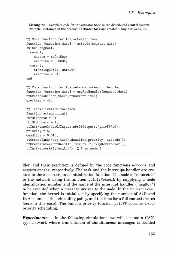
7.5 Examples

Listing 7.4 Complete code for the actuator node in the distributed control systemexample. Instances of the aperiodic actuator task are created using ttCreateJob.

%% Code function for the actuator task

function [exectime,data] = actcode(segment,data)

switch segment,

case 1,

data.u = ttGetMsg;

exectime = 0.0005;

case 2,

ttAnalogOut(1, data.u);

exectime = -1;

end

%% Code function for the network interrupt handler

function [exectime,data] = msgRcvHandler(segment,data)

ttCreateJob(’act_task’,ttCurrentTime);

exectime = -1;

%% Initialization function

function actuator_init

nbrOfInputs = 0;

nbrOfOutputs = 1;

ttInitKernel(nbrOfInputs,nbrOfOutputs,’prioFP’,0);

priority = 5;

deadline = 0.010;

ttCreateTask(’act_task’,deadline,priority,’actcode’);

ttCreateInterruptHandler(’msgRcv’,1,’msgRcvHandler’);

ttInitNetwork(2,’msgRcv’); % I am node 2

dler, and their execution is defined by the code functions actcode andmsgRcvHandler, respectively. The task and the interrupt handler are cre­ated in the actuator_init initialization function. The node is “connected”to the network using the function ttInitNetwork by supplying a nodeidentification number and the name of the interrupt handler (’msgRcv’)to be executed when a message arrives to the node. In the ttInitKernelfunction, the kernel is initialized by specifying the number of A/D andD/A channels, the scheduling policy, and the time for a full context switch(zero in this case). The built­in priority function prioFP specifies fixed­priority scheduling.

Experiments. In the following simulations, we will assume a CAN­type network where transmission of simultaneous messages is decided

155

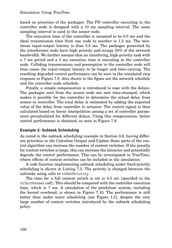
Simulation Using TrueTime

based on priorities of the packages. The PD controller executing in thecontroller node is designed with a 10 ms sampling interval. The samesampling interval is used in the sensor node.The execution time of the controller is assumed to be 0.5 ms and the

ideal transmission time from one node to another is 1.5 ms. The min­imum input­output latency is thus 3.5 ms. The packages generated bythe interference node have high priority and occupy 50% of the networkbandwidth. We further assume that an interfering, high­priority task witha 7 ms period and a 3 ms execution time is executing in the controllernode. Colliding transmissions and preemption in the controller node willthus cause the input­output latency to be longer and time­varying. Theresulting degraded control performance can be seen in the simulated stepresponse in Figure 7.8. Also shown in the figure are the network scheduleand the controller node schedule.Finally, a simple compensation is introduced to cope with the delays.

The packages sent from the sensor node are now time­stamped, whichmakes it possible for the controller to determine the actual delay fromsensor to controller. The total delay is estimated by adding the expectedvalue of the delay from controller to actuator. The control signal is thencalculated based on linear interpolation among a set of controller param­eters precalculated for different delays. Using this compensation, bettercontrol performance is obtained, as seen in Figure 7.9.

Example 2: Subtask Scheduling

As noted in the subtask scheduling example in Section 3.6, having differ­ent priorities in the Calculate Output and Update State parts of the con­trol algorithm can increase the number of context switches. If the penaltyfor context switches is large, this can increase the latencies and potentiallydegrade the control performance. This can be investigated in TrueTime,where effects of context switches can be included in the simulation.A code function implementing subtask scheduling under fixed­priority

scheduling is shown in Listing 7.5. The priority is changed between thesubtasks using calls to ttSetPriority.The time for a full context switch is set to 0.5 ms (specified in the

ttInitKernel call). This should be compared with the controller executiontime, which is 7 ms. A simulation of the pendulum system, includingthe kernel overhead, is shown in Figure 7.10. The performance is stillbetter than under naive scheduling (see Figure 1.3), despite the verylarge number of context switches introduced by the subtask schedulingpolicy.

156

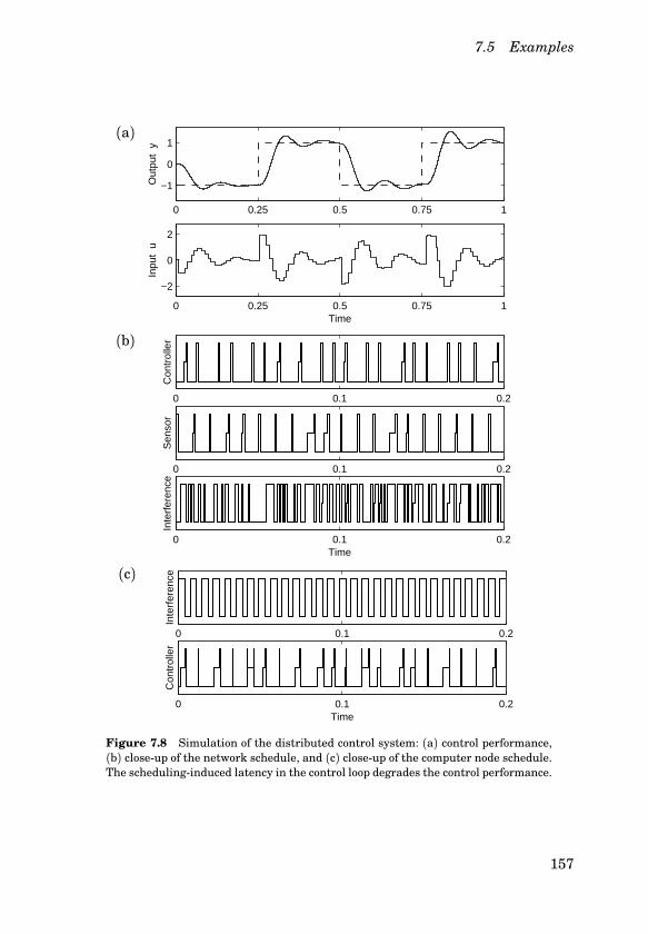
7.5 Examples

(a)

0 0.25 0.5 0.75 1

−1

0

1O

utpu

t y

0 0.25 0.5 0.75 1

−2

0

2

Inpu

t u

Time

(b)

0 0.1 0.2

Inte

rfer

ence

Time

0 0.1 0.2

Sen

sor

0 0.1 0.2

Con

trol

ler

(c)

0 0.1 0.2

Con

trol

ler

Time

0 0.1 0.2

Inte

rfer

ence

Figure 7.8 Simulation of the distributed control system: (a) control performance,(b) close­up of the network schedule, and (c) close­up of the computer node schedule.The scheduling­induced latency in the control loop degrades the control performance.

157

Simulation Using TrueTime

0 0.25 0.5 0.75 1

−1

0

1

Out

put

y

0 0.25 0.5 0.75 1

−2

0

2

Inpu

t u

Time

Figure 7.9 Simulation of the distributed control system with scheduling­induceddelays and delay­compensation. The performance is improved compared to Fig­ure 7.8.

Example 3: Execution-Time Estimation

The feedback scheduler introduced in Chapter 4 requires that the execu­tion times of the various tasks can be measured. Functionality to mea­sure execution times is provided in TrueTime through the use of budgets.When a task instance is created, the budget is set to the declared WCETof the task. As the task executes, the budget is decreased by the sameamount. When the task finishes, the actual execution time of the taskinstance can be found by comparing the remaining budget to the WCET.Execution­time estimation using a forgetting factor (see Eq. (4.1)) can beperformed in a custom finish hook (see Section 7.3) that can be reusedfor all tasks. Assuming that the task user data structure (task->data)has two fields called Chat (the estimate) and lambda (the forgetting fac­tor), a finish hook implementing the execution­time estimation is shownin Listing 7.6.

Example 4: Server-Based Scheduling

Server­based scheduling (see Section 2.2) can be used to limit the utiliza­tion of aperiodic tasks, or tasks that have unknown or unbounded exe­cution time. In Chapter 5, modified constant bandwidth servers (CBSs)were used to provide isolation between unrelated tasks in the ControlServer model. In TrueTime, general server mechanisms can be imple­mented through the use of scheduling hooks and timers. This requiresknowledge about the internal workings of the kernel and also that somecustom C++ code is written.More simple server mechanisms can be implemented using task bud­

gets and execution­time overrun handlers. In this example, we will limit

158

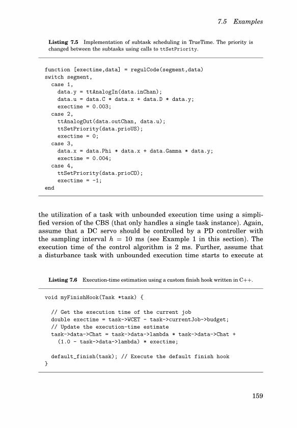
7.5 Examples

Listing 7.5 Implementation of subtask scheduling in TrueTime. The priority ischanged between the subtasks using calls to ttSetPriority.

function [exectime,data] = regulCode(segment,data)

switch segment,

case 1,

data.y = ttAnalogIn(data.inChan);

data.u = data.C * data.x + data.D * data.y;

exectime = 0.003;

case 2,

ttAnalogOut(data.outChan, data.u);

ttSetPriority(data.prioUS);

exectime = 0;

case 3,

data.x = data.Phi * data.x + data.Gamma * data.y;

exectime = 0.004;

case 4,

ttSetPriority(data.prioCO);

exectime = -1;

end

the utilization of a task with unbounded execution time using a simpli­fied version of the CBS (that only handles a single task instance). Again,assume that a DC servo should be controlled by a PD controller withthe sampling interval h = 10 ms (see Example 1 in this section). Theexecution time of the control algorithm is 2 ms. Further, assume thata disturbance task with unbounded execution time starts to execute at

Listing 7.6 Execution­time estimation using a custom finish hook written in C++.

void myFinishHook(Task *task) {

// Get the execution time of the current job

double exectime = task->WCET - task->currentJob->budget;

// Update the execution-time estimate

task->data->Chat = task->data->lambda * task->data->Chat +

(1.0 - task->data->lambda) * exectime;

default_finish(task); // Execute the default finish hook

}

159

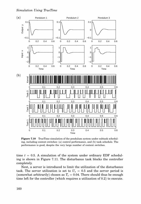
Simulation Using TrueTime

(a)

0 0.2 0.4 0.6

−0.1

0

0.1O

utpu

t y

Pendulum 1

0 0.2 0.4 0.6

−0.1

0

0.1

Pendulum 2

0 0.2 0.4 0.6

−0.1

0

0.1

Pendulum 3

0 0.2 0.4 0.6

−2

−1

0

1

Time

Inpu

t u

0 0.2 0.4 0.6

−2

−1

0

1

Time0 0.2 0.4 0.6

−2

−1

0

1

Time

(b)

0 0.1 0.2 0.3 0.4 0.5 0.6

Tas

k 1

Time

0 0.1 0.2 0.3 0.4 0.5 0.6

Tas

k 2

0 0.1 0.2 0.3 0.4 0.5 0.6

Tas

k 3

0 0.1 0.2 0.3 0.4 0.5 0.6

Ker

nel

Figure 7.10 TrueTime simulation of the pendulum system under subtask schedul­ing, including context switches: (a) control performance, and (b) task schedule. Theperformance is good, despite the very large number of context switches.

time t = 0.5. A simulation of the system under ordinary EDF schedul­ing is shown in Figure 7.11. The disturbance task blocks the controllercompletely.Next, a server is introduced to limit the utilization of the disturbance

task. The server utilization is set to Us = 0.5 and the server period is(somewhat arbitrarily) chosen as Ts = 0.04. There should thus be enoughtime left for the controller (which requires a utilization of 0.2) to execute.

160

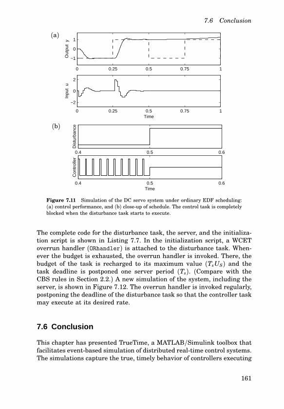
7.6 Conclusion

(a)

0 0.25 0.5 0.75 1

−1

0

1

Out

put

y

0 0.25 0.5 0.75 1

−2

0

2

Inpu

t u

Time

(b)

0.4 0.5 0.6

Con

trol

ler

Time

0.4 0.5 0.6

Dis

turb

ance

Figure 7.11 Simulation of the DC servo system under ordinary EDF scheduling:(a) control performance, and (b) close­up of schedule. The control task is completelyblocked when the disturbance task starts to execute.

The complete code for the disturbance task, the server, and the initializa­tion script is shown in Listing 7.7. In the initialization script, a WCEToverrun handler (ORhandler) is attached to the disturbance task. When­ever the budget is exhausted, the overrun handler is invoked. There, thebudget of the task is recharged to its maximum value (TsUS) and thetask deadline is postponed one server period (Ts). (Compare with theCBS rules in Section 2.2.) A new simulation of the system, including theserver, is shown in Figure 7.12. The overrun handler is invoked regularly,postponing the deadline of the disturbance task so that the controller taskmay execute at its desired rate.

7.6 Conclusion

This chapter has presented TrueTime, a MATLAB/Simulink toolbox thatfacilitates event­based simulation of distributed real­time control systems.The simulations capture the true, timely behavior of controllers executing

161

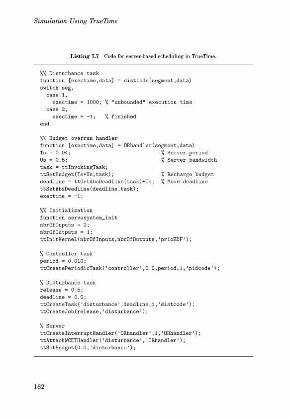
Simulation Using TrueTime

Listing 7.7 Code for server­based scheduling in TrueTime.

%% Disturbance task

function [exectime,data] = distcode(segment,data)

switch seg,

case 1,

exectime = 1000; % "unbounded" execution time

case 2,

exectime = -1; % finished

end

%% Budget overrun handler

function [exectime,data] = ORhandler(segment,data)

Ts = 0.04; % Server period

Us = 0.5; % Server bandwidth

task = ttInvokingTask;

ttSetBudget(Ts*Us,task); % Recharge budget

deadline = ttGetAbsDeadline(task)+Ts; % Move deadline

ttSetAbsDeadline(deadline,task);

exectime = -1;

%% Initialization

function servosystem_init

nbrOfInputs = 2;

nbrOfOutputs = 1;

ttInitKernel(nbrOfInputs,nbrOfOutputs,’prioEDF’);

% Controller task

period = 0.010;

ttCreatePeriodicTask(’controller’,0.0,period,1,’pidcode’);

% Disturbance task

release = 0.5;

deadline = 0.0;

ttCreateTask(’disturbance’,deadline,1,’distcode’);

ttCreateJob(release,’disturbance’);

% Server

ttCreateInterruptHandler(’ORhandler’,1,’ORhandler’);

ttAttachWCETHandler(’disturbance’,’ORhandler’);

ttSetBudget(0.0,’disturbance’);

162

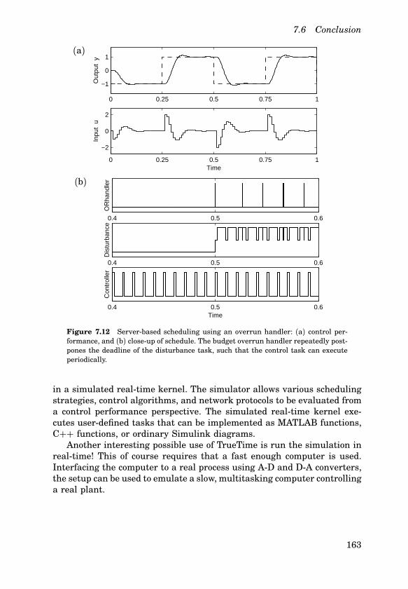
7.6 Conclusion

(a)

0 0.25 0.5 0.75 1

−1

0

1

Out

put

y

0 0.25 0.5 0.75 1

−2

0

2

Inpu

t u

Time

(b)

0.4 0.5 0.6

Con

trol

ler

Time

0.4 0.5 0.6

Dis

turb

ance

0.4 0.5 0.6

OR

hand

ler

Figure 7.12 Server­based scheduling using an overrun handler: (a) control per­formance, and (b) close­up of schedule. The budget overrun handler repeatedly post­pones the deadline of the disturbance task, such that the control task can executeperiodically.

in a simulated real­time kernel. The simulator allows various schedulingstrategies, control algorithms, and network protocols to be evaluated froma control performance perspective. The simulated real­time kernel exe­cutes user­defined tasks that can be implemented as MATLAB functions,C++ functions, or ordinary Simulink diagrams.Another interesting possible use of TrueTime is run the simulation in

real­time! This of course requires that a fast enough computer is used.Interfacing the computer to a real process using A­D and D­A converters,the setup can be used to emulate a slow, multitasking computer controllinga real plant.

163

8

Conclusion

8.1 Summary

The design of a real­time control system is essentially a codesign prob­lem. Decisions made in the real­time design affect the control design, andvice versa. For instance, the choice of scheduling policy influences the la­tency distributions in the control loops, and, ideally, this should be takeninto account in the control design. At the same time, the performance re­quirements of the individual control loops place demands on the real­timesystem with regard to, e.g., sampling periods and latencies. This thesishas dealt with various aspects of the control and scheduling codesignproblem. The work has fallen into two main categories: the developmentof tools for analysis of control timing, and the development of schedulingtechniques tailored to control tasks.

Tools for Analysis of Control Timing

A multitasking real­time control system is a very complex system. Thereare interactions between the continuous­time plant dynamics, the controltasks, and the real­time scheduling algorithm. In order to understand andanalyze these systems, new software tools are needed. This thesis has pre­sented two such tools: Jitterbug (Chapter 6) and TrueTime (Chapter 7).

Analysis Using Jitterbug. Controllers are often designed with littleregard for the real­time implementation. Using the MATLAB­based tool­box Jitterbug, the control performance degradation due to slow samplingand scheduling­induced input­output latency and jitter can be computedanalytically. The control system is built from a number of linear systems,and the performance is evaluated by a quadratic cost function. A stochas­tic timing model with random delays is used to describe the execution

164

8.1 Summary

of the controller in each period. The tool can be used at early stages inthe design process to determine how sensitive a controller is to timingvariations. Being quite general, Jitterbug is applicable to a wide range ofproblems within control and signal processing.

Simulation Using TrueTime. The MATLAB/Simulink­based simula­tor TrueTime can be used to investigate real­time control systems in moredetail. The control tasks are described by arbitrary code functions (writ­ten as MATLAB functions, C++ functions, or Simulink block diagrams),while the plant dynamics can be modeled using the full power of Simulink.In TrueTime, the internal workings of real­time kernels and communica­tions networks are simulated in parallel with the plant. Unlike Jitterbug,the tool allows for time­domain responses and transient phenomena (inboth scheduling and control) to be studied. Also, nonlinear systems maybe studied. The various scheduling techniques presented in the thesis (seebelow) have all been developed and evaluated with the aid of TrueTime.

Scheduling Techniques Tailored to Control Tasks

Vast amounts of scheduling theory has been developed over the last deca­des, but very little of it is tailored to control tasks. It has been pointedout that the performance of a controller depends on the sampling interval,the input­output latency, and the sampling and input­output jitter. Usingsubtask scheduling (Chapter 3), the input­output latency can be reduced.Feedback scheduling was introduced in Chapter 4 to dynamically adjustthe sampling periods, optimizing the overall performance. The ControlServer (Chapter 5) combines ideas from the previous chapters to createcontrol tasks with both predictable and adjustable performance.

Subtask Scheduling. Scheduling the two main parts of a control algo­rithm (Calculate Output and Update State) as separate tasks, it is possi­ble to reduce the input­output latency (and jitter) in a set of control tasks.Deadline assignment—something which is seldom treated in the schedul­ing literature—has been considered under both fixed­priority (FP) andearliest­deadline­first (EDF) scheduling. Subtask scheduling under EDFis one of the ideas behind the Control Server.

Feedback Scheduling. A simple feedback scheduling strategy hasbeen developed, where the sampling periods of a set of control tasks areadjusted based on execution­time measurements. The goal has been tokeep a high CPU utilization, providing high control performance despitevariations in the execution time of the control algorithms. Simulationcase studies on hybrid and linear controllers have been presented. Thesimulations have mainly assumed FP scheduling, which is unfair to the

165

Conclusion

lowest­priority tasks. Better performance is obtained using EDF schedul­ing. An even better alternative is to use Control Servers, which facilitateexact resource distribution among the tasks.

The Control Server. A new computational model for control tasks,called the Control Server model, has been proposed. The Control Servercreates the abstraction of a control task with a specified sampling periodand a constant input­output latency (shorter than the period), makingit possible to account for the latency in the control design. Tasks maybe combined into more complex components without loss of their indi­vidual fixed­latency properties. Based on the constant bandwidth server,the Control Server also provides isolation between unrelated tasks. Im­plementation of the Control Server requires that the real­time operatingsystem supports earliest­deadline­first scheduling.

8.2 Suggestions for Future Work

The current work can be extended in many directions. Some suggestionsfor future work are given below.

Overrun Handling. A topic that has not received much attention isthe problem of task overruns. What should be done if a control task doesnot finish before the deadline? Many alternatives exist: the task could beaborted, the computations could continue in the next period, an alterna­tive action could be taken, etc. The problem becomes especially intricatewhen the control algorithm has been divided into segments. For instance,should the Update State part be executed even if the Calculate Outputpart was aborted (or did not finish in time)? Are some controller realiza­tions more sensitive to aborted computations than others? The ControlServer model could be extended to allow various overrun handling meth­ods to be specified for different tasks.

Feedback Scheduling Structures. The feedback scheduling structureproposed in this thesis is only one of many possible. Other variables thanthe CPU utilization could be controlled, for instance the latency and jitterin each control loop. The resource distribution should ideally be based onthe current performance of the controllers, and not just a stationary costfunction. Move involved schemes could be developed, where the schedulerand the controllers negotiate for available resources at regular intervals.

Scheduling of Anytime Controllers. An interesting class of con­trollers that require new scheduling techniques are anytime controllers.

166

8.2 Suggestions for Future Work

In such controllers, the quality of the control signal is gradually refinedas the execution progresses. A good example is model­predictive control(MPC), where an optimization problem is solved by iterative techniquesin each sample. To reach the optimum, very long execution times may beneeded. Terminating the optimization early, acceptable results may stillbe obtained. There is an interesting trade­off between the input­outputlatency (due to the long execution time) and the quality of the controlsignal. A preliminary study on scheduling of MPCs is presented in [Hen­riksson et al., 2002].

Control­Theoretic Issues. Jitter and changes of sampling intervalsdue to dynamic scheduling strategies lead to many interesting control­theoretical issues. Are there analytical results regarding the sensitivityof a controller towards jitter? Can a controller be designed to be robustagainst both sampling jitter and input­output jitter?In feedback scheduling applications, the performance of a controller

should ideally be measured using a non­stationary cost function that re­flects the current status of the plant. How should these cost functions beformulated?

Scheduling of Networks. In distributed control systems, the networkbandwidth may be the bottleneck resource, and not the CPU time in thenodes. Similar to the CPU scheduling case, the network resources could bedynamically distributed among several competing control loops. Networktransmissions are typically nonpreemptive, and this makes the schedulingproblem more difficult. Also, the feedback mechanism may need to bedistributed among the nodes in the network. TrueTime is currently beingextended to simulate higher­level network protocols such as TCP.

Implementation Issues. The feedback scheduler and the Control Ser­ver presented in the thesis assume that task execution times can be mea­sured in the real­time operating system. Furthermore, the Control Serveris based on EDF scheduling. Currently, these features are not availablein many RTOSs. The Control Server was implemented in a public domainreal­time kernel [Andersson and Blomdell, 1991]. An alternative would beto base the implementation on the open source RTLinux kernel, which caneasily be modified to use EDF, e.g., [Vidal et al., 2002]. Another promisingimplementation platform is Real­Time Java [Bollella et al., 2000], which,according to the specification, supports both execution­time measurementsand various scheduling policies. Currently, there is no known Real­TimeJava implementation that supports EDF scheduling, however.

167

Appendix

Cost Calculation in Example 3.1

The delayed integrator process can be written

dx(t)dt

= u(t− L) + vc(t), 0 ≤ L ≤ h, (A.1)

where L is the input­output latency, and h is the sampling interval. Thecost function to be minimized can be written

J = 1hE

{∫ h

0x2(t) dt

}

. (A.2)

Inserting the process description (A.1) into (A.2) gives

J = 1hE

{

∫ L

0

(

x(kh) + tu(kh− h) +∫ t

0vc(s)ds

)2

dt

+∫ h

L

(

x(kh) + Lu(kh− h) + (t− L)u(kh) +∫ t

0vc(s)ds

)2

dt

}

= 1hE

x(kh)u(kh− h)u(kh)

T

Q1 Q12

QT12 Q2

x(kh)u(kh− h)u(kh)

+ Jsamp,

(A.3)

where

Q1 =

hL2

2+ (h−L)L

L2

2+ (h−L)L L3

3+ (h−L)L2

, Q12 =

(h−L)22

(h−L)22

L

,

168

Cost Calculation in Example 3.1

Q2 = (h−L)33

, Jsamp = 1h

∫ h

0

∫ t

01ds dt = h/2.

Sampling the process (A.1) with the interval h gives

x(kh+ h)u(kh)

= Φ

x(kh)u(kh− h)

+ Γu(kh) + v(kh), (A.4)

where

Φ =

1 L

0 0

, Γ =

h− L1

,

and v is a discrete­time white noise process with covariance

R =

h 0

0 0

.

Introduce the positive definite matrix S. The controller that minimizes thecost satisfies the algebraic Riccati equation (e.g. [Åström and Wittenmark,1997])

S = ΦTSΦ + Q1 −(

ΦTSΓ + Q12)(

ΓTSΓ + Q2)−1(

ΓTSΦ + QT12)

, (A.5)

with the solution

S =

L +√3 h6

L

6

(

3L −√3 h

)

L

6

(

3L −√3 h

) L3

3−

√3 L2h6

.

The optimal control law is

u(kh) = −K

x(kh)u(kh− h)

, (A.6)

where

K =(

Q2 + ΓTSΓ)−1(

ΓTSΦ + QT12)

=

1h

√3+ 32+

√3

L

h

√3+ 32+

√3

,

and the optimal cost is given by

J = 1htr SR + Jsamp = 3+

√3

6h+ L. (A.7)

169

Appendix

Proof of Theorem 4.2

The release time of job number k of task i is kTi + φ i. The deadline of jobnumber k of task i is kTi + φ i + Di. Let ki(t) be the number of finishedjobs of task i at time t. After a while, CPU is never idle, therefore,

Iidle(t) +∑

i

(ki(t)Ci + ei(t)) = t, (A.8)

where Iidle(t) is the accumulated idle time, ei is how long the currentinvocation of task i has executed. Both Iidle(t) and ei are bounded and0 ≤ ei ≤ Ci. Furthermore, due to the overload situation, tasks are finishedin the order of their deadlines. Therefore,

kl(t)Tl + Dl + φ l ≤ (ki(t) + 1)Ti + Di + φ i. (A.9)

(Otherwise task l would not have finished job number kl(t) before task ifinished job number ki(t) + 1). Symmetrically,

ki(t)Ti + Di + φ i ≤ (kl(t) + 1)Tl + Dl + φ l . (A.10)

The two equations above give

kl(t)Tl + Dl + φ l − Ti ≤ ki(t)Ti + Di + φ i ≤ (kl(t) + 1)Tl + Dl + φ l . (A.11)

Hence,

kl(t)Tl + Dl − Ti + φ lkl(t)Tl

≤ ki(t)Ti + Di + φ ikl(t)Tl

≤ (kl(t) + 1)Tl + Dl + φ lkl(t)Tl

.

(A.12)Here, the limit of the left­hand side and the right­hand side are both equalto one, so,

limt→∞

kj(t)Tjkl(t)Tl

= 1. (A.13)

170

Proof of Theorem 4.2

Rearranging the terms in (A.8) and letting t→ ∞, we have

1 = limt→∞1t

∑

i

ki(t)Ci

= limt→∞1t

∑

i

ki(t)TiCi

Ti

= limt→∞

∑

j kj(t)Tjt

∑

i

ki(t)Ti∑

j kj(t)TjCi

Ti

= limt→∞

ki(t)Ti∑

jkj(t)Tjki(t)Ti

t

∑

i

1∑

jkj(t)Tjki(t)Ti

Ci

Ti

= limt→∞

ki(t)Tint

∑

i

1n

Ci

Ti

= limt→∞

ki(t)Tit

∑

i

Ci

Ti.

(A.14)

Hence,

Ti = limt→∞

t

ki(t)= Ti

∑

j

Cj

Tj= TiU . (A.15)

171

References

Abdelzaher, T. F., E. M. Atkins, and K. Shin (2000): “QoS negotiationin real­time systems and its application to automated flight control.”IEEE Transactions on Computers, 49:11, pp. 1170–1183.

Abeni, L. (1998): “Server mechanisms for multimedia applications.”Technical Report RETIS TR98­01. Scuola Superiore S. Anna, Pisa,Italy.

Abeni, L. and G. Buttazzo (1998): “Integrating multimedia applications inhard real­time systems.” In Proceedings of the 19th IEEE Real­TimeSystems Symposium. Madrid, Spain.

Abeni, L. and G. Buttazzo (1999): “Adaptive bandwidth reservationfor multimedia computing.” In Proceedings of the 6th InternationalConference on Real­Time Computing Systems and Applications. HongKong, P.R. China.

Abeni, L., L. Palopoli, G. Lipari, and J. Walpole (2002): “Analysis ofa reservation­based feedback scheduler.” In Proceedings of the 23rdIEEE Real­Time Systems Symposium.

Agrawal, M., D. Cofer, and T. Samad (2003): “Real­time adaptive resourcemanagement for advanced avionics.” IEEE Control Systems Magazine,23:1, pp. 76–86.

Albertos, P. and A. Crespo (1999): “Real­time control of non­uniformlysampled systems.” Control Engineering Practice, 7, pp. 445–458.

Albertos, P., A. Crespo, I. Ripoll, M. Vallés, and P. Balbastre (2000):“RT control scheduling to reduce control performance degrading.” InProceedings of the 39th IEEE Conference on Decision and Control.Sydney, Australia.

Andersson, L. and A. Blomdell (1991): “A real­time programming envi­ronment and a real­time kernel.” In Asplund, Ed., National Swedish

172

Symposium on Real­Time Systems, Technical Report No 30 1991­06­21. Dept. of Computer Systems, Uppsala University, Uppsala, Sweden.

Åström, K. J. and B. Wittenmark (1997): Computer­Controlled Systems.Prentice Hall.

Audsley, N., A. Burns, M. Richardson, and A. Wellings (1994): “STRESS—A simulator for hard real­time systems.” Software—Practice andExperience, 24:6, pp. 543–564.

Audsley, N., K. Tindell, and A. Burns (1993): “The end of the line for staticcyclic scheduling.” In Proceedings of the 5th Euromicro Workshop onReal­Time Systems.

Balbastre, P., I. Ripoll, and A. Crespo (2000): “Control task delay reductionunder static and dynamic scheduling policies.” In Proceedings of the7th International Conference on Real­Time Computing Systems andApplications.

Baruah, S., G. Buttazzo, S. Gorinsky, and G. Lipari (1999a): “Schedulingperiodic task systems to minimize output jitter.” In Proceedings of the6th International Conference on Real­Time Computing Systems andApplications.

Baruah, S., D. Chen, and A. Mok (1999b): “Static­priority scheduling ofmulti­frame tasks.” In Proceedings of the 11th Euromicro Conferenceon Real­Time Systems.

Beccari, G., S. Caselli, M. Reggiani, and F. Zanichelli (1999): “Rate modu­lation of soft real­time tasks in autonomous robot control systems.” InProceedings of the 11th Euromicro Conference on Real­Time Systems,pp. 21–28. York, England.

Bhattacharyya, S. S., E. Cheong, J. Davis II, M. Goel, C. Hylands,B. Kienhuis, E. A. Lee, J. Liu, X. Liu, L. Muliadi, S. Neuendorffer,J. Reekie, N. Smyth, J. Tsay, B. Vogel, W. Williams, Y. Xiong, andH. Zheng (2002): “Heterogeneous concurrent modeling and design inJava.” Technical Report UCB/ERL M02/23. Dept. EECS, Universityof California at Berkeley.

Blevins, P. and C. Ramamoorthy (1976): “Aspects of a dynamicallyadaptive operating system.” IEEE Transactions on Computers, 25:7,pp. 713–725.

Bollella, G., B. Brosgol, P. Dibble, S. Furr, J. Gosling, D. Hardin, andM. Turnbull (2000): The Real­Time Specification for Java. Addison­Wesley.

173

References

Brück, D., H. Elmqvist, S. E. Mattsson, and H. Olsson (2002): “Dymolafor multi­engineering modeling and simulation.” In Proceedings of the2nd International Modelica Conference.

Burns, A., D. Prasad, A. Bondavalli, F. D. Giandomenico, K. Ramam­ritham, J. Stankovc, and L. Stringini (2000): “The meaning and roleof value in scheduling flexible real­time systems.” Journal of SystemsArchitecture, 46, pp. 305–325.

Burns, A., K. Tindell, and A. J. Wellings (1994): “Fixed priority schedulingwith deadlines prior to completion.” In Proceedings of the 6th Euromi­cro Workshop on Real­Time Systems, pp. 138–142.

Burns, A. and A. Wellings (2001): Real­Time Systems and ProgrammingLanguages, 3rd edition. Addison­Wesley.

Buttazzo, G., G. Lipari, and L. Abeni (1998): “Elastic task model foradaptive rate control.” In Proceedings of the 19th IEEE Real­TimeSystems Symposium, pp. 286–295.

Buttazzo, G. C. (1997): Hard Real­Time Computing Systems: PredictableScheduling Algorithms and Applications. Kluwer Academic Publishers.

Caccamo, M., G. Buttazzo, and L. Sha (2000a): “Capacity sharing foroverrun control.” In Proceedings of the IEEE Real­Time SystemsSymposium. Orlando, Florida.

Caccamo, M., G. Buttazzo, and L. Sha (2000b): “Elastic feedback control.”In Proceedings of the 12th Euromicro Conference on Real­TimeSystems, pp. 121–128. Stockholm, Sweden.

Casile, A., G. Buttazzo, G. Lamastra, and G. Lipari (1998): “Simulationand tracing of hybrid task sets on distributed systems.” In Proceedingsof the 5th International Conference on Real­Time Computing Systemsand Applications.

Crespo, A., I. Ripoll, and P. Albertos (1999): “Reducing delays in RTcontrol: The control action interval.” In Proceedings of the 14th IFACWorld Congress, pp. 257–262.

Crnkovic, I. and M. Larsson, Eds. (2002): Building Relable Component­Based Software Systems. Artech House Publishers.

Eker, J. and A. Cervin (1999): “A Matlab toolbox for real­time and controlsystems co­design.” In Proceedings of the 6th International Conferenceon Real­Time Computing Systems and Applications, pp. 320–327. HongKong, P.R. China.

174

Eker, J., A. Cervin, and A. Hörjel (2001): “Distributed wireless controlusing Bluetooth.” In Proceedings of the IFAC Conference on NewTechnologies for Computer Control. Hong Kong, P.R. China.

Eker, J., P. Hagander, and K.­E. Årzén (2000): “A feedback scheduler forreal­time control tasks.” Control Engineering Practice, 8:12, pp. 1369–1378.

Eker, J. and J. Malmborg (1999): “Design and implementation of a hybridcontrol strategy.” IEEE Control Systems Magazine, 19:4.

El­khoury, J. and M. Törngren (2001): “Towards a toolset for architecuraldesign of distributed real­time control systems.” In Proceedings of the22nd IEEE Real­Time Systems Symposium.

Fletcher, R. (1987): Practical Methods of Optimization. Wiley.Gerber, R. and S. Hong (1993): “Semantics­based compiler transforma­tions for enhanced schedulability.” In Proceedings of the 14th IEEEReal­Time Systems Symposium, pp. 232–242.

Gerber, R. and S. Hong (1997): “Slicing real­time programs for enhancedschedulabilty.” ACM Transactions on Programming Languages andSystems, 19:3, pp. 525–555.

Gerber, R., S. Hong, and M. Saksena (1995): “Guaranteeing real­timerequirements with resource­based calibration of periodic processes.”IEEE Trans on Software Engineering, 21:7.

Gill, C. D., D. L. Levine, and D. C. Schmidt (1998): “Dynamic schedulingstrategies for avionics mission computing.” In Proceedings of the 17thIEEE/AIAA Digital Avionics Systems Conference.

Gutierrez, J. and M. Harbour (1998): “Schedulability analysis for taskswith static and dynamic offsets.” In Proceedings of the 19th IEEEReal­Time Systems Symposium.

Hägglund, T. (1992): “A predictive PI controller for processes with longdead times.” IEEE Control Systems Magazine, 12:1, pp. 57–60.

Halang, W. (1993): “Achieving jitter­free and predictable real­time con­trol by accurately timed computer peripherals.” Control EngineeringPractice, 1:6, pp. 979–987.

Harbour, M. G., M. G., M. H. Klein, and J. P. Lehoczky (1994): “Timinganalysis for fixed­priority scheduling of hard real­time systems.” IEEETransactions on Software Engineering, 20:1, pp. 13–28.

175

References

Henriksson, D. and A. Cervin (2003): “TrueTime 1.1—Reference manual.”Technical Report ISRN LUTFD2/TFRT­­7605­­SE. Department ofAutomatic Control, Lund Institute of Technology, Sweden.

Henriksson, D., A. Cervin, J. Åkesson, and K.­E. Årzén (2002): “Feedbackscheduling of model predictive controllers.” In Proceedings of the8th IEEE Real­Time and Embedded Technology and ApplicationsSymposium. San Jose, CA.

Henzinger, T. A., B. Horowitz, and C. M. Kirsch (2001): “Giotto: A time­triggered language for embedded programming.” In Proceedings of theFirst International Workshop on Embedded Software.

Jeffay, K. and D. L. Stone (1993): “Accounting for interrupt handling costsin dynamic priority systems.” In Proceedings of the 14th IEEE Real­Time Systems Symposium.

Ji, Y., H. Chizeck, X. Feng, and K. Loparo (1991): “Stability and controlof discrete­time jump linear systems.” Control­Theory and AdvancedApplications, 7:2, pp. 247–270.

Joseph, M. and P. Pandya (1986): “Finding response times in a real­timesystem.” The Computer Journal, 29:5, pp. 390–395.

Klein, M. H., T. Ralya, B. Pollak, R. Obenza, and M. Gonzalez Härbour(1993): A Practitioner’s Handbook for Real­Time Analysis: Guide toRate Monotonic Analysis for Real­Time Systems. Kluwer AcademicPublisher.

Kleinrock, L. (1970): “A continuum of time­sharing scheduling algo­rithms.” In AFIPS Conference Proceedings, Spring Joint ComputerConference, pp. 453–458.

Krasovskii, N. and E. Lidskii (1961): “Analytic design of controllers insystems with random attributes, I, II, III.” Automation and RemoteControl, 22:9–11, pp. 1021–1025, 1141–1146, 1289–1294.

Krishna, C. M. and K. G. Shin (1997): Real­Time Systems. McGraw­Hill.Lehoczky, J., L. Sha, and J. Strosnider (1987): “Enhanced apriodicresponsiveness in hard real­time environment.” In Proceedings of the8th IEEE Real­Time Systems Symposium.

Leung, J. Y. T. and J. Whitehead (1982): “On the complexity of fixed­priority scheduling of periodic, real­time tasks.” Performance Evalua­tion, 2:4, pp. 237–250.

Li, B. and K. Nahrstedt (1998): “A control theoretical model for quality ofservice adaptations.” In Proceedings of the 6th International Workshopon Quality of Service, pp. 145–153.

176

Lincoln, B. (2002a): “Jitter compensation in digital control systems.” InProceedings of the 2002 American Control Conference.

Lincoln, B. (2002b): “A simple stability criterion for control systems withvarying delays.” In Proceedings of the 15th IFAC World Congress.

Lincoln, B. and B. Bernhardsson (2000): “Efficient pruning of search treesin LQR control of switched linear systems.” In Proceedings of theConference on Decision and Control.

Lipari, G. and S. Baruah (2000): “Greedy reclamation of unused band­width in constant­bandwidth servers.” In Proceedings of the EuromicroConference on Real­Time Systems. Stockholm, Sweden.

Liu, C. L. and J. W. Layland (1973): “Scheduling algorithms for multi­programming in a hard­real­time environment.” Journal of the ACM,20:1, pp. 40–61.

Liu, J. and E. Lee (2003): “Timed multitasking for real­time embeddedsoftware.” IEEE Control Systems Magazine, 23:1.

Liu, J. W. S. (2000): Real­Time Systems. Prentice Hall.Locke, C. D. (1992): “Software architecture for hard real­time appli­cations: Cyclic vs. fixed priority executives.” Real­Time Systems, 4,pp. 37–53.

Lu, C., J. Stankovic, T. Abdelzaher, G. Tao, S. Son, and M. Marley(2000): “Performance specifications and metrics for adaptive real­time systems.” In Proceedings of the 21st IEEE Real­Time SystemsSymposium, pp. 13–23.

Lu, C., J. Stankovic, G. Tao, and S. H. Son (1999): “Design and evaluationof a feedback control EDF scheduling algorithm.” In Proceedings of the20th IEEE Real­Time Systems Symposium, pp. 56–67.

Lu, C., J. A. Stankovic, S. H. Son, and G. Tao (2002): “Feedback controlreal­time scheduling: framework, modeling and algorithms.” Real­Time Systems, 23:1/2, pp. 85–126.

Marti, P., G. Fohler, K. Ramamritham, and J. M. Fuertes (2001): “Jittercompensation for real­time control systems.” In Proceedings of the22nd IEEE Real­Time Systems Symposium.

MathWorks (2001): Simulink: A Program for Simulating DynamicSystems—User’s Guide. The MathWorks Inc.

Nilsson, J. (1998a): Real­Time Control Systems with Delays. PhD thesisISRN LUTFD2/TFRT­­1049­­SE, Department of Automatic Control,Lund Institute of Technology, Sweden.

177

References

Nilsson, J. (1998b): “Two toolboxes for systems with random delays.”Technical Report ISRN LUTFD2/TFRT­­7572­­SE. Department ofAutomatic Control, Lund Institute of Technology, Sweden.

Palopoli, L., L. Abeni, and G. Buttazzo (2000): “Real­time control systemanalysis: An integrated approach.” In Proceedings of the 21st IEEEReal­Time Systems Symposium.

Palopoli, L., C. Pinello, A. Sangiovanni­Vincentelli, L. El­Ghaoui, andA. Bicchi (2002): “Synthesis of robust control systems under resourceconstraints.” In Proceedings of the Workshop on Hybrid Systems:Computation and Control.

Parekh, A. and R. Gallager (1993): “A generalized processor sharingapproach to flow control in integrated services networks: the singlenode case.” IEEE/ACM Transactions on Networking, 1:3, pp. 344–357.

Persson, P., A. Cervin, and J. Eker (2000): “Execution­time properties ofa hybrid controller.” Technical Report ISRN LUTFD2/TFRT­­7591­­SE. Department of Automatic Control, Lund Institute of Technology,Sweden.

Potier, D., E. Gelenbe, and J. Lenfant (1976): “Adaptive allocation ofcentral processing unit quanta.” Journal of the ACM, 23:1, pp. 97–102.

Rajkumar, R., C. Lee, J. Lehoczky, and D. Siewiorek (1997): “A resourcesallocation model for QoS management.” In Proceedings of the 18thIEEE Real­Time Systems Symposium, pp. 298–307.

Redell, O. and M. Sanfridson (2002): “Exact best­case response timeanalysis of fixed priority scheduled tasks.” In Proceedings of the 14thEuromicro Conference on Real­Time Systems. Vienna, Austria.

Redell, O. and M. Törngren (2002): “Calculating exact worst­case reponsetimes for static priority scheduled tasks with offsets and jitter.” InProceedings of the IEEE Real­Time and Embedded Technology andApplications Symposium. San Jose, California.

Rehbinder, H. and M. Sanfridson (2000): “Integration of off­line schedul­ing and optimal control.” In Proceedings of the 12th Euromicro Con­ference on Real­Time Systems.

Ryu, M. and S. Hong (1998): “Toward automatic synthesis of schedulablereal­time controllers.” Integrated Computer­Aided Engineering, 5:3,pp. 261–277.

178

Ryu, M., S. Hong, and M. Saksena (1997): “Streamlining real­time con­troller design: From performance specifications to end­to­end timingconstraints.” In Proceedings of the 3rd IEEE Real­Time Technologyand Applications Symposium, pp. 91–99.

Seto, D., J. P. Lehoczky, L. Sha, and K. G. Shin (1996): “On taskschedulability in real­time control systems.” In Proceedings of the 17thIEEE Real­Time Systems Symposium, pp. 13–21. Washington, DC.

Shin, K. and C. Meissner (1999): “Adaptation of control system perfor­mance by task reallocation and period modification.” In Proceedings ofthe 11th Euromicro Conference on Real­Time Systems, pp. 29–36.

Sprunt, B., L. Sha, and J. Lehoczky (1989): “Aperiodic task schedulingfor hard real­time systems.” Real­Time Systems.

Spuri, M. and G. Buttazzo (1996): “Scheduling aperiodic tasks in dynamicpriority systems.” Real­Time Systems, 10:2, pp. 179–210.

Stankovic, J. A., C. Lu, S. H. Son, and G. Tao (1999): “The case forfeedback control real­time scheduling.” In Proceedings of the 11thEuromicro Conference on Real­Time Systems, pp. 11–20.

Stankovic, J. A., M. Spuri, K. Ramamritham, and G. C. Buttazzo(1998): Deadline Scheduling for Real­Time Systems—EDF and RelatedAlgorithms. Kluwer Academic Publishers.

Storch, M. F. and J. W.­S. Liu (1996): “DRTSS: A simulation frameworkfor complex real­time systems.” In Proceedings of the 2nd IEEE Real­Time Technology and Applications Symposium.

Vidal, J., A. Crespo, and P. Balbastre (2002): “Control task implementa­tion in rtlinux.” In Proceedings of the 15th IFAC World Congress.

Wittenmark, B. and K. J. Åström (1980): “Simple self­tuning controllers.”In Unbehauen, Ed., Methods and Applications in Adaptive Control,number 24 in Lecture Notes in Control and Information Sciences,pp. 21–29. Springer­Verlag, Berlin, FRG.

Zhao, Q. C. and D. Z. Zheng (1999): “Stable and real­time scheduling of aclass of hybrid dynamic systems.” Journal of Discrete Event DynamicalSystems, 9:1, pp. 45–64.

179