Integrated analysis of land-use, energy and watersystems for ethanol production from sugarcane inBoliviaJenny Gabriela Pena Balderrama  ( gabrie@kth.se )

Royal Institute of Technology, KTHDilip Khatiwada 

Royal Institute of Technology, KTHFrancesco Gardumi 

Royal Institute of Technology, KTHThomas Alfstad 

United Nations Division of Social and Economic AffairsSilvia Ulloa Jimenez 

Stockholm Environment InstituteMark Howells 

Loughborough University https://orcid.org/0000-0001-6419-4957

Article

Keywords: Biomass, Road Transport Sector, Production Chain Sustainability, Least-cost OptimizationModel, Agricultural Intensi�cation

Posted Date: November 11th, 2020

DOI: https://doi.org/10.21203/rs.3.rs-97263/v2

License: This work is licensed under a Creative Commons Attribution 4.0 International License.  Read Full License

1

Integrated analysis of land-use, energy and water systems

for ethanol production from sugarcane in Bolivia

J. Gabriela Peña-Balderrama1,2*, Dilip Khatiwada1, Francesco Gardumi1,, Thomas Alfstad3, Silvia Ulloa-Jimenez4, Mark Howells5,6

1 KTH Royal Institute of Technology, Department of Energy Technology, Stockholm, Sweden; gabrie@kth.se;

dilip.khatiwada@energy.kth.se, gardumi@kth.se. 2 Universidad Mayor de San Simón, Facultad de Ciencias y Tecnología, Cochabamba, Bolivia. 3 United Nations Division of Social and Economic Affairs, New York, USA; thomas.alfstad@un.org. 4 Stockholm Environment Institute, Massachusetts, USA; silvia.ulloa@sei.org. 5 Department of Geography, Loughborough University, UK; m.i.howells@lboro.ac.uk. 6 Centre for Environmental Policy, Imperial College London, UK, m.i.howells@lboro.ac.uk. * Correspondence: gabrie@kth.se; Tel.: +46-076-408-8437

Abstract 1

The use of biomass for renewable energy production is one alternative to reduce the environmental 2 impacts of energy production worldwide. Sugarcane-based ethanol is one of the most widespread biofuels 3 in the road transport sector and its development has been encouraged by strong incentives on production 4 and use in several countries. The growing realization on the environmental impacts of ethanol production 5 indicates the need to increase the efficient utilization of biomass resources by optimizing the production 6 chain sustainably. This paper evaluates enhancements in the ethanol production chain quantitatively by 7 identifying opportunities for agricultural intensification and investments in advanced biorefineries in a 8 least-cost optimization model. Results of our model show that significant cost and environmental benefits 9 can be achieved by modernizing sugarcane agriculture in Bolivia. Demands for ethanol and sugar can be 10 met cost-effectively by increasing sugarcane yields from the current country-average of 55.34 ton/ha to 11 85.7 ton/ha in 2030 with a moderate cropland expansion of 11.4 thousand hectares in the period 2019-12 2030. Our results further suggest that it is cost-optimal to invest in efficient cogeneration in biorefineries 13 to maximize the renewable energy output and the economic benefits of sugarcane ethanol. Finally, biofuel 14 support in the range of 8-10 US$/GJ is required for investments in second-generation ethanol in 15 biorefineries to be cost-competitive in the medium-term. 16

1 Introduction 17

Biofuels are an alternative for meeting the world's increasing energy needs and can contribute to 18 mitigate greenhouse gas (GHG) emissions and to increase the sustainability of global energy production 19 1,2. Depending on the feedstock used for their production, biofuels can be categorized into first, second 20 and third generation. Feedstock for first-generation biofuels are limited to edible crops, such as grains 21 (maize, sorghum and wheat), sugar crops (sugarcane and sugar beet), starch crops (cassava) and oilseed 22 crops (soy, palm, rapeseed) 3. In contrast, second-generation biofuels are produced from non-edible crops, 23 including lignocellulosic residues from agriculture and forestry 4. Third-generation biofuels are produced 24 from algae, sewage sludge, and municipal solid wastes 5. 25

Worldwide, ethanol is the most widely used biofuel in the transport sector. In 2019, the global ethanol 26 production reached 110.4 billion liters (72% v/v of the global liquid biofuel production) 6 and it is expected 27 to increase to 143 billion liters by 2028 7. Among the main feedstock sources for ethanol production (corn, 28 sugarcane, wheat, sugar beet and sorghum), sugarcane is the most effective option in terms of GHG 29 emissions savings, energy requirements from fossil fuels (energy balance) and land requirements 3. 30 Sugarcane-based ethanol produced under sustainable conditions has clear advantages over gasoline in 31 reducing GHG emissions and improving air quality in metropolitan areas 8. Today, ethanol replaces 32 approximately 2% (in energy basis) of the gasoline consumed worldwide and it is projected to supply the 33 14% of global ethanol production by 2028 6,7. 34

2

In order to promote sustainable sugarcane-based ethanol production, several aspects within the supply 1 chain must be assessed. These include feedstock production 9–13, industrial production of ethanol 14–16, 2 water quality and availability 17–19, the energy balance and carbon footprint 20–23. In this article, important 3 aspects of sustainable ethanol production, viz. agricultural production of sugarcane (e.g. land use, 4 agricultural inputs) and the industrial production of ethanol in biorefineries (e.g. conversion efficiency, 5 costs) are evaluated. 6

There is a large potential to enhance the environmental benefits of ethanol production from sugarcane 7 by increasing efficiency in the agricultural production chain (increasing yields, restricting biomass 8 residues burning and using abandoned residues/wastes to produce bioenergy, among others) and thereby 9 reducing the environmental impacts 3,22,23. Reducing the gap between the actual and potential yield can be 10 achieved by reducing growth limiting factors (water and nutrients deficit) and growth reducing factors 11 (pests, diseases, weeds, insects and pollutants) by the use of irrigation, fertilization and the use of 12 agrochemicals, respectively 11,24,25. Also, agricultural mechanization can contribute to increase 13 productivity on account of timeliness of operations and more efficient utilization of agricultural inputs 14 and labor, providing environmental and economic benefits 13,26–28. 15

Higher energy yields and emissions reductions can be achieved for electricity generation and/or 16 second-generation ethanol production through the utilization of lignocellulosic residues, i.e. surplus 17 bagasse and agricultural residues (tops and trashes) 14,15,29,30. Advanced cogeneration systems lead to a 18 reduction in steam consumption, providing higher electricity generation and export potential compared to 19 traditional cogeneration systems 31–33. Further process optimization can integrate the biochemical 20 processing of surplus lignocellulosic residues for second-generation ethanol production 14,29,34. Other 21 alternative technologies to increase the electricity generation potential include the biomass integrated 22 gasifier combined cycle, BIGCC, with further surplus electricity potential of more than 250 kWh/tc 16,35. 23

This study aims to examine potential yield improvements in sugarcane production systems using a 24 tiered approach of agricultural management levels/practices (see Section 3.3) and to evaluate alternative 25 uses of sugarcane biomass residues for bioelectricity and second-generation ethanol production (see 26 Section 3.4). The study performs techno-economic optimization to evaluate cost-optimal upgrades of 27 agricultural production systems and to evaluate the location and size of different biorefinery 28 configurations. A lifecycle approach is performed to compare (in terms of energy inputs/outputs, lifecycle 29 emissions and costs) six agricultural production systems and four biorefinery configurations. In addition, 30 an integrated multi-resource modelling approach allows evaluating pressures on land and water resources. 31 The methodology is tested on a case study assessing biofuel production targets, together with land use, 32 agricultural production, and energy security in Bolivia. The suggested approach is based on open-source 33 modelling tools and can therefore be applied to other countries where biofuel production is under 34 development. 35

Following this introductory section, context information is provided. Section 2 introduces the case 36 study in Bolivia. Section 3 introduces the methods and models used in the analysis. Results are presented 37 and discussed in Section 4. Finally, concluding remarks and policy implications are described in Section 38 5. 39

2 Country context 40

To reduce its dependence on liquid fuel imports (diesel and gasoline) and to achieve greater energy 41 security, the government of Bolivia promulgated the Law N°1098/2018 to initiate liquid biofuel 42 production and blending. In 2018, an agreement between the government and the private sector (sugar 43 producers) aimed to produce 80 million liters of anhydrous ethanol in that year, with the expectation to 44 reach 380 million liters in 2025 36. The ethanol blending mandate started with 10% in 2018 and should 45 gradually increase to 25% by 2025 36. In current agreements, ethanol is to be produced using sugarcane 46 as feedstock, and the ethanol blends are mandated to increase, displacing gradually pure gasoline available 47 in the market. 48

To reach the production targets, the government of Bolivia estimates to expand the sugarcane 49 cultivated area in 155 thousand hectares in the period 2018-2025, nearly duplicating the 172.6 thousand 50

3

hectares harvested in 2019 36,37. In 2019, the country-average sugarcane yield was 55.3 tons per hectare 1 (t/ha) which is low compared to its average potential yield of 116 t/ha 1 38. In addition, the latest national 2 Census on agriculture indicates that 96.4% of the sugarcane cultivated is rainfed, therefore sensitive to 3 variations in precipitation. Several producers have narrowed the country-average yield gap with advanced 4 agricultural management practices and increased mechanization. However, further investments in 5 sustainable intensification 10,39 are required to meet the increasing demands of sugar and ethanol with 6 fewer land resources. 7

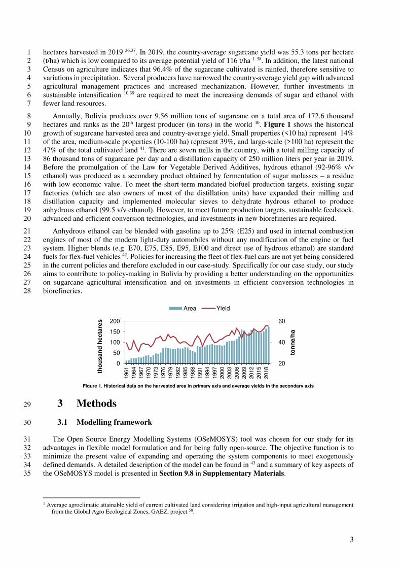
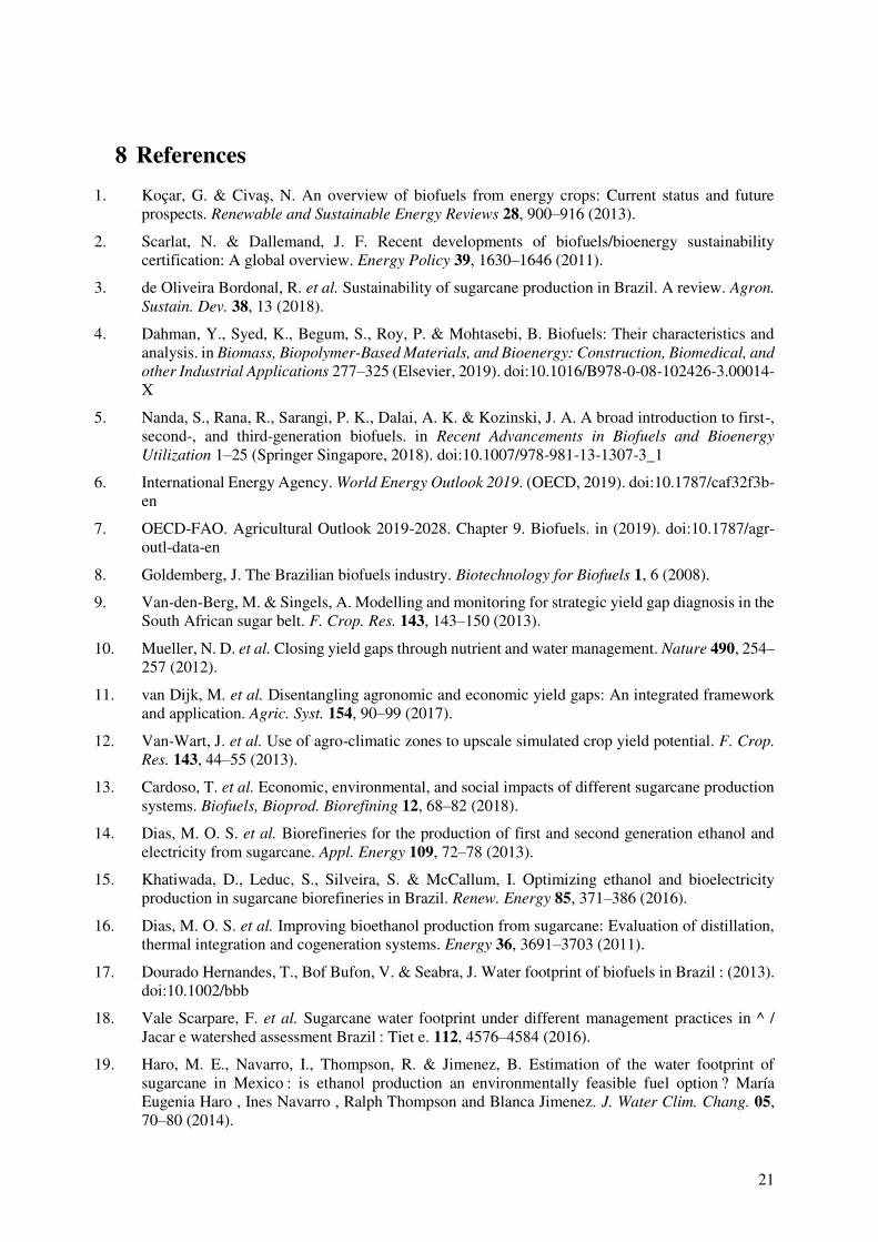
Annually, Bolivia produces over 9.56 million tons of sugarcane on a total area of 172.6 thousand 8 hectares and ranks as the 20th largest producer (in tons) in the world 40. Figure 1 shows the historical 9 growth of sugarcane harvested area and country-average yield. Small properties (<10 ha) represent 14% 10 of the area, medium-scale properties (10-100 ha) represent 39%, and large-scale (>100 ha) represent the 11 47% of the total cultivated land 41. There are seven mills in the country, with a total milling capacity of 12 86 thousand tons of sugarcane per day and a distillation capacity of 250 million liters per year in 2019. 13 Before the promulgation of the Law for Vegetable Derived Additives, hydrous ethanol (92-96% v/v 14 ethanol) was produced as a secondary product obtained by fermentation of sugar molasses – a residue 15 with low economic value. To meet the short-term mandated biofuel production targets, existing sugar 16 factories (which are also owners of most of the distillation units) have expanded their milling and 17 distillation capacity and implemented molecular sieves to dehydrate hydrous ethanol to produce 18 anhydrous ethanol (99.5 v/v ethanol). However, to meet future production targets, sustainable feedstock, 19 advanced and efficient conversion technologies, and investments in new biorefineries are required. 20

Anhydrous ethanol can be blended with gasoline up to 25% (E25) and used in internal combustion 21 engines of most of the modern light-duty automobiles without any modification of the engine or fuel 22 system. Higher blends (e.g. E70, E75, E85, E95, E100 and direct use of hydrous ethanol) are standard 23 fuels for flex-fuel vehicles 42. Policies for increasing the fleet of flex-fuel cars are not yet being considered 24 in the current policies and therefore excluded in our case-study. Specifically for our case study, our study 25 aims to contribute to policy-making in Bolivia by providing a better understanding on the opportunities 26 on sugarcane agricultural intensification and on investments in efficient conversion technologies in 27 biorefineries. 28

Figure 1. Historical data on the harvested area in primary axis and average yields in the secondary axis

3 Methods 29

3.1 Modelling framework 30

The Open Source Energy Modelling Systems (OSeMOSYS) tool was chosen for our study for its 31 advantages in flexible model formulation and for being fully open-source. The objective function is to 32 minimize the present value of expanding and operating the system components to meet exogenously 33 defined demands. A detailed description of the model can be found in 43 and a summary of key aspects of 34 the OSeMOSYS model is presented in Section 9.8 in Supplementary Materials. 35

1 Average agroclimatic attainable yield of current cultivated land considering irrigation and high-input agricultural management

from the Global Agro Ecological Zones, GAEZ, project 58.

20

40

60

0

50

100

150

200

1961

1964

1967

1970

1973

1976

1979

1982

1985

1988

1991

1994

1997

2000

2003

2006

2009

2012

2015

2018

ton

ne

/ha

tho

us

an

d h

ec

tare

s

Area Yield

4

Although OSeMOSYS was conceived as a modelling tool for energy systems analysis, its structure 1 allows for modelling any type of system. OSeMOSYS has been widely used in studies of multi-resource 2 integrated systems models (CLEWs), in which interlinkages between land-use systems (L), energy 3 systems (E), water systems (W), and effects of climate (C) are studied in conjunction 44. A recent literature 4 review by Pereira-Ramos et al. shows 23 CLEWs nexus applications using the OSeMOSYS modelling 5 tool 45. 6

In our study, the CLEWs framework was used to assess nexus interactions between the agriculture 7 sector and biorefineries with the water and energy systems. Section 3.7 details the nexus interactions 8 captured in the model. 9

3.2 Model timeframe, spatial zonation and system boundaries 10

The selected modelling timeframe is from 2013 to 2030, with a temporal resolution of one year. Since 11 the study focuses on evaluating improvements in the agricultural production of sugarcane, the base year 12 is calibrated to represent data found in statistics of the latest National Agricultural Census (year 2013, 13 each agricultural Census is conducted every ten years approximately). The end year is set 5 years after 14 the end of the medium-term ethanol production targets to further explore investment needs in the medium-15 term. 16

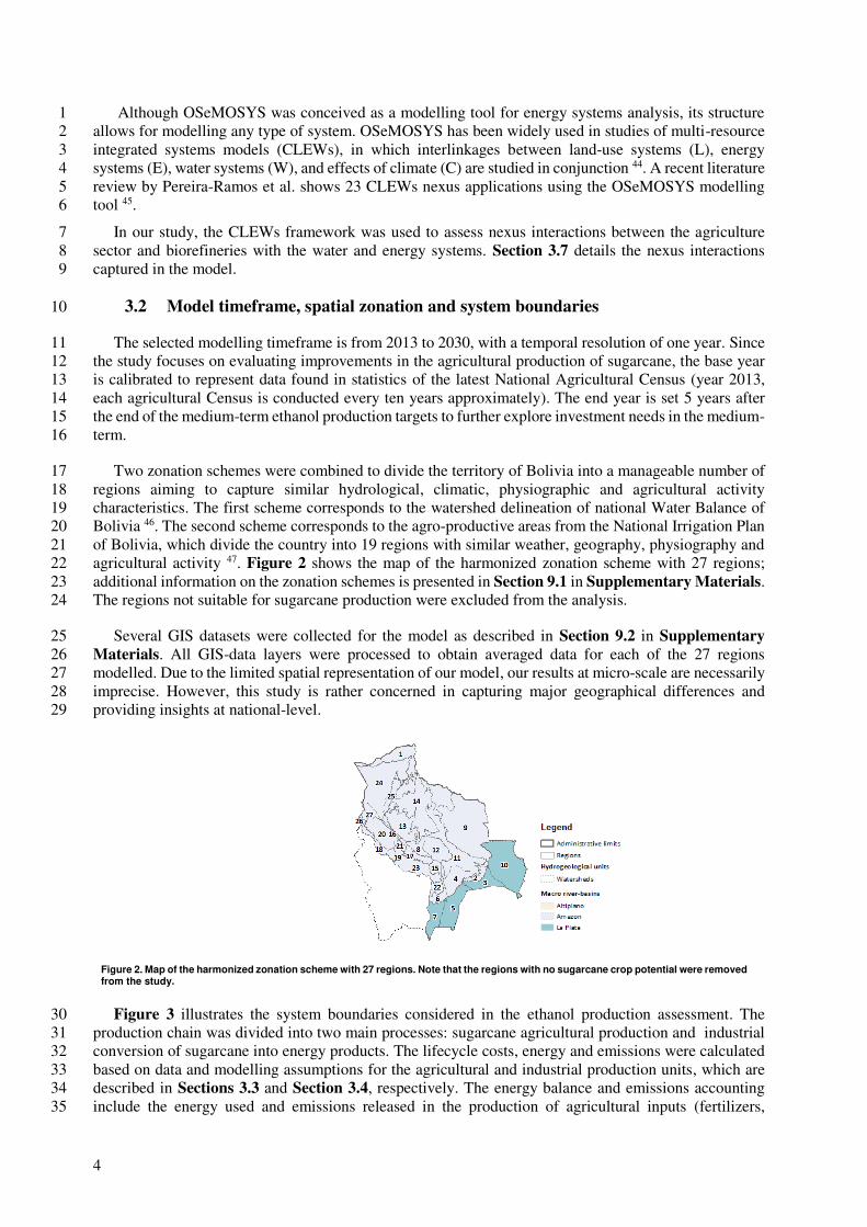
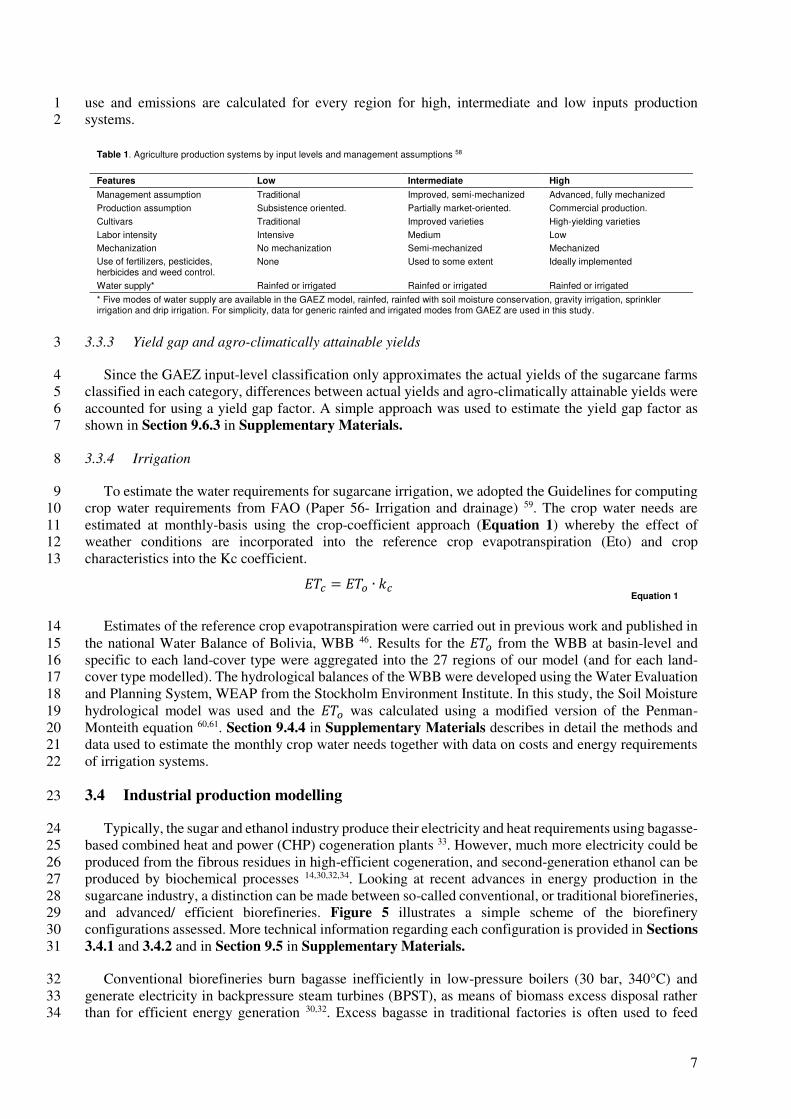
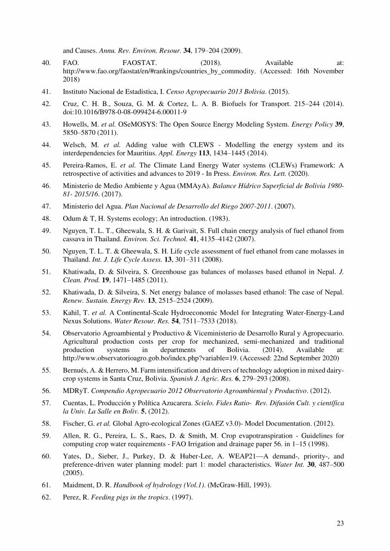
Two zonation schemes were combined to divide the territory of Bolivia into a manageable number of 17 regions aiming to capture similar hydrological, climatic, physiographic and agricultural activity 18 characteristics. The first scheme corresponds to the watershed delineation of national Water Balance of 19 Bolivia 46. The second scheme corresponds to the agro-productive areas from the National Irrigation Plan 20 of Bolivia, which divide the country into 19 regions with similar weather, geography, physiography and 21 agricultural activity 47. Figure 2 shows the map of the harmonized zonation scheme with 27 regions; 22 additional information on the zonation schemes is presented in Section 9.1 in Supplementary Materials. 23 The regions not suitable for sugarcane production were excluded from the analysis. 24

Several GIS datasets were collected for the model as described in Section 9.2 in Supplementary 25 Materials. All GIS-data layers were processed to obtain averaged data for each of the 27 regions 26 modelled. Due to the limited spatial representation of our model, our results at micro-scale are necessarily 27 imprecise. However, this study is rather concerned in capturing major geographical differences and 28 providing insights at national-level. 29

Figure 2. Map of the harmonized zonation scheme with 27 regions. Note that the regions with no sugarcane crop potential were removed from the study.

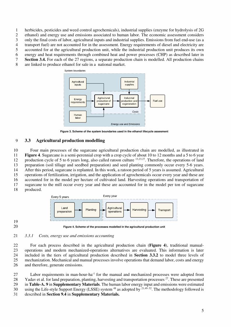
Figure 3 illustrates the system boundaries considered in the ethanol production assessment. The 30 production chain was divided into two main processes: sugarcane agricultural production and industrial 31 conversion of sugarcane into energy products. The lifecycle costs, energy and emissions were calculated 32 based on data and modelling assumptions for the agricultural and industrial production units, which are 33 described in Sections 3.3 and Section 3.4, respectively. The energy balance and emissions accounting 34 include the energy used and emissions released in the production of agricultural inputs (fertilizers, 35

5

herbicides, pesticides and weed control agrochemicals), industrial supplies (enzyme for hydrolysis of 2G 1 ethanol) and energy use and emissions associated to human labor. The economic assessment considers 2 only the final costs of labor, agricultural inputs and industrial supplies. Emissions from fuel end-use (as a 3 transport fuel) are not accounted for in the assessment. Energy requirements of diesel and electricity are 4 accounted for at the agricultural production unit, while the industrial production unit produces its own 5 energy and heat requirements through combined heat and power processes (CHP) as described later in 6 Section 3.4. For each of the 27 regions, a separate production chain is modelled. All production chains 7 are linked to produce ethanol for sale in a national market. 8

Figure 3. Scheme of the system boundaries used in the ethanol lifecycle assesment

3.3 Agricultural production modelling 9

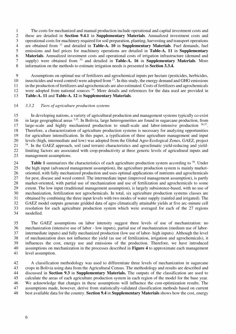
Four main processes of the sugarcane agricultural production chain are modelled, as illustrated in 10 Figure 4. Sugarcane is a semi-perennial crop with a crop cycle of about 10 to 12 months and a 5 to 6 year 11 production cycle of 5 to 6 years long, also called ratoon culture 13,23,27. Therefore, the operations of land 12 preparation (soil tillage and seedbed preparation) and seed planting commonly occur every 5-6 years. 13 After this period, sugarcane is replanted. In this work, a ratoon period of 5 years is assumed. Agricultural 14 operations of fertilization, irrigation, and the application of agrochemicals occur every year and these are 15 accounted for in the model per hectare of cultivated land. Harvesting operations and transportation of 16 sugarcane to the mill occur every year and these are accounted for in the model per ton of sugarcane 17 produced. 18

19 Figure 4. Scheme of the processes modelled in the agricultural production unit 20

3.3.1 Costs, energy use and emissions accounting 21

For each process described in the agricultural production chain (Figure 4), traditional manual-22 operations and modern mechanized-operations alternatives are evaluated. This information is later 23 included in the tiers of agricultural production described in Section 3.3.2 to model three levels of 24 mechanization. Mechanical and manual processes involve operations that demand labor, costs and energy 25 and therefore, generate emissions. 26

Labor requirements in man-hour-ha-1 for the manual and mechanized processes were adopted from 27 Yadav et al. for land preparation, planting, harvesting and transportation processes 27. These are presented 28 in Table-A. 9 in Supplementary Materials. The human labor energy input and emissions were estimated 29 using the Life-style Support Energy (LSSE) system 48 as adopted by 21,49–52. The methodology followed is 30 described in Section 9.4 in Supplementary Materials. 31

6

The costs for mechanized and manual production include operational and capital investment costs and 1 these are detailed in Section 9.4.1 in Supplementary Materials. Annualized investment costs and 2 operational costs for machinery required for soil preparation, planting, harvesting and transport operations 3 are obtained from 13 and detailed in Table-A. 10 in Supplementary Materials. Fuel demands, fuel 4 emissions and fuel prices for machinery operations are detailed in Table-A. 11 in Supplementary 5 Materials. Annualized investment costs and operational costs of irrigation infrastructure (demand and 6 supply) were obtained from 53 and detailed in Table-A. 16 in Supplementary Materials. More 7 information on the methods to estimate irrigation needs is presented in Section 3.3.4. 8

Assumptions on optimal use of fertilizers and agrochemical inputs per hectare (pesticides, herbicides, 9 insecticides and weed control) were adopted from 23. In this study, the energy demand and GHG emissions 10 in the production of fertilizers and agrochemicals are also estimated. Costs of fertilizers and agrochemicals 11 were adopted from national sources 54. More details and references for the data used are provided in 12 Table-A. 11 and Table-A. 12 in Supplementary Materials. 13

3.3.2 Tiers of agriculture production systems 14

In developing nations, a variety of agricultural production and management systems typically co-exist 15 in large geographical areas 3,55. In Bolivia, large heterogeneities are found in sugarcane production, from 16 large-scale and highly mechanized production to small-scale and labor-intensive production 56,57. 17 Therefore, a characterization of agriculture production systems is necessary for analyzing opportunities 18 for agriculture intensification. In this paper, a typification of three agriculture management and input 19 levels (high, intermediate and low) was adopted from the Global Agro-Ecological Zones, GAEZ, project 20 58. In the GAEZ approach, soil (and terrain) characteristics and agroclimatic yield-reducing and yield-21 limiting factors are associated with crop-productivity at three generic levels of agricultural inputs and 22 management assumptions. 23

Table 1 summarizes the characteristics of each agriculture production system according to 58. Under 24 the high input (advanced management assumption), the agriculture production system is mainly market-25 oriented, with fully mechanized production and uses optimal applications of nutrients and agrochemicals 26 for pest, disease and weed control. The intermediate input (improved management assumption), is partly 27 market-oriented, with partial use of mechanization and use of fertilization and agrochemicals to some 28 extent. The low input (traditional management assumption), is largely subsistence-based, with no use of 29 mechanization, fertilization nor agrochemicals. In total, six agriculture production systems classes are 30 obtained by combining the three input levels with two modes of water supply (rainfed and irrigated). The 31 GAEZ model outputs generate gridded data of agro climatically attainable yields at five arc-minute cell 32 resolution for each agriculture production system which were averaged for each of the 27 regions 33 modelled. 34

The GAEZ assumptions on labor intensity suggest three levels of use of mechanization: no 35 mechanization (intensive use of labor - low inputs), partial use of mechanization (medium use of labor- 36 intermediate inputs) and fully mechanized production (low use of labor- high inputs). Although the level 37 of mechanization does not influence the yield (as use of fertilization, irrigation and agrochemicals), it 38 influences the cost, energy use and emissions of the production. Therefore, we have introduced 39 assumptions on mechanization in the processes described in Figure 4 to approximate each management 40 level assumption. 41

A classification methodology was used to differentiate three levels of mechanization in sugarcane 42 crops in Bolivia using data from the Agricultural Census. The methodology and results are described and 43 discussed in Section 9.3 in Supplementary Materials. The outputs of the classification are used to 44 calculate the areas of each agriculture production system in each region of the model for the base year. 45 We acknowledge that changes in these assumptions will influence the cost-optimization results. The 46 assumptions made, however, derive from statistically-validated classification methods based on current 47 best available data for the country. Section 9.4 in Supplementary Materials shows how the cost, energy 48

7

use and emissions are calculated for every region for high, intermediate and low inputs production 1 systems. 2

Table 1. Agriculture production systems by input levels and management assumptions 58

Features Low Intermediate High

Management assumption Traditional Improved, semi-mechanized Advanced, fully mechanized

Production assumption Subsistence oriented. Partially market-oriented. Commercial production.

Cultivars Traditional Improved varieties High-yielding varieties

Labor intensity Intensive Medium Low

Mechanization No mechanization Semi-mechanized Mechanized

Use of fertilizers, pesticides, herbicides and weed control.

None Used to some extent Ideally implemented

Water supply* Rainfed or irrigated Rainfed or irrigated Rainfed or irrigated

* Five modes of water supply are available in the GAEZ model, rainfed, rainfed with soil moisture conservation, gravity irrigation, sprinkler irrigation and drip irrigation. For simplicity, data for generic rainfed and irrigated modes from GAEZ are used in this study.

3.3.3 Yield gap and agro-climatically attainable yields 3

Since the GAEZ input-level classification only approximates the actual yields of the sugarcane farms 4 classified in each category, differences between actual yields and agro-climatically attainable yields were 5 accounted for using a yield gap factor. A simple approach was used to estimate the yield gap factor as 6 shown in Section 9.6.3 in Supplementary Materials. 7

3.3.4 Irrigation 8

To estimate the water requirements for sugarcane irrigation, we adopted the Guidelines for computing 9 crop water requirements from FAO (Paper 56- Irrigation and drainage) 59. The crop water needs are 10 estimated at monthly-basis using the crop-coefficient approach (Equation 1) whereby the effect of 11 weather conditions are incorporated into the reference crop evapotranspiration (Eto) and crop 12 characteristics into the Kc coefficient. 13 𝐸𝑇𝑐 = 𝐸𝑇𝑜 ∙ 𝑘𝑐

Equation 1

Estimates of the reference crop evapotranspiration were carried out in previous work and published in 14 the national Water Balance of Bolivia, WBB 46. Results for the 𝐸𝑇𝑜 from the WBB at basin-level and 15 specific to each land-cover type were aggregated into the 27 regions of our model (and for each land-16 cover type modelled). The hydrological balances of the WBB were developed using the Water Evaluation 17 and Planning System, WEAP from the Stockholm Environment Institute. In this study, the Soil Moisture 18 hydrological model was used and the 𝐸𝑇𝑜 was calculated using a modified version of the Penman-19 Monteith equation 60,61. Section 9.4.4 in Supplementary Materials describes in detail the methods and 20 data used to estimate the monthly crop water needs together with data on costs and energy requirements 21 of irrigation systems. 22

3.4 Industrial production modelling 23

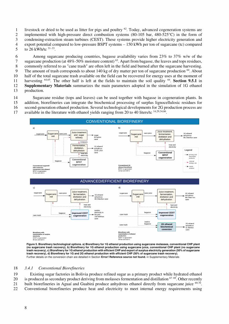
Typically, the sugar and ethanol industry produce their electricity and heat requirements using bagasse-24 based combined heat and power (CHP) cogeneration plants 33. However, much more electricity could be 25 produced from the fibrous residues in high-efficient cogeneration, and second-generation ethanol can be 26 produced by biochemical processes 14,30,32,34. Looking at recent advances in energy production in the 27 sugarcane industry, a distinction can be made between so-called conventional, or traditional biorefineries, 28 and advanced/ efficient biorefineries. Figure 5 illustrates a simple scheme of the biorefinery 29 configurations assessed. More technical information regarding each configuration is provided in Sections 30 3.4.1 and 3.4.2 and in Section 9.5 in Supplementary Materials. 31

Conventional biorefineries burn bagasse inefficiently in low-pressure boilers (30 bar, 340°C) and 32 generate electricity in backpressure steam turbines (BPST), as means of biomass excess disposal rather 33 than for efficient energy generation 30,32. Excess bagasse in traditional factories is often used to feed 34

8

livestock or dried to be used as litter for pigs and poultry 62. Today, advanced cogeneration systems are 1 implemented with high-pressure direct combustion systems (80-105 bar, 480-525°C) in the form of 2 condensing-extraction steam turbines (CEST). These systems provide higher electricity generation and 3 export potential compared to low-pressure BSPT systems – 150 kWh per ton of sugarcane (tc) compared 4 to 26 kWh/tc 31–33. 5

Among sugarcane producing countries, bagasse availability varies from 23% to 37% w/w of the 6 sugarcane production (at 48%-50% moisture content) 63. Apart from bagasse, the leaves and tops residues, 7 commonly referred to as "cane trash" are often left in the field and burned after the sugarcane harvesting. 8 The amount of trash corresponds to about 140 kg of dry matter per ton of sugarcane production 64. About 9 half of the total sugarcane trash available on the field can be recovered for energy uses at the moment of 10 harvesting 64,65. The other half is left at the fields to maintain the soil quality 64. Section 9.5.1 in 11 Supplementary Materials summarizes the main parameters adopted in the simulation of 1G ethanol 12 production. 13

Sugarcane residue (tops and leaves) can be used together with bagasse in cogeneration plants. In 14 addition, biorefineries can integrate the biochemical processing of surplus lignocellulosic residues for 15 second-generation ethanol production. Several technological developments for 2G production process are 16 available in the literature with ethanol yields ranging from 20 to 40 liters/tc 14,29,34,66. 17

Figure 5. Biorefinery technological options. a) Biorefinery for 1G ethanol production using sugarcane molasses, conventional CHP plant (no sugarcane trash recovery), b) Biorefinery for 1G ethanol production using sugarcane juice, conventional CHP plant (no sugarcane trash recovery), c) Biorefinery for 1G ethanol production with efficient CHP and export of surplus electricity generation (50% of sugarcane trash recovery), d) Biorefinery for 1G and 2G ethanol production with efficient CHP (50% of sugarcane trash recovery).

Further details on the conversion chain are detailed in Section Error! Reference source not found. in Supplementary Materials

3.4.1 Conventional Biorefineries 18

Existing sugar factories in Bolivia produce refined sugar as a primary product while hydrated ethanol 19 is produced as secondary product deriving from molasses fermentation and distillation 67–69. Other recently 20 built biorefineries in Aguaí and Guabirá produce anhydrous ethanol directly from sugarcane juice 69,70. 21 Conventional biorefineries produce heat and electricity to meet internal energy requirements using 22

9

conventional cogeneration. For simplicity, the small amount of surplus electricity generated (in the range 1 of 10-26 kWh/ton cane) 22 is neglected in our study. 2

Although some sugar factories operate in flexible conditions – by adjusting their production of sugar 3 and ethanol to market and supply/demand conditions 21 – we have introduced fixed production ratios for 4 the sake of simplicity. Conventional technologies for ethanol production were divided into two 5 configurations, as presented in Figure 5.a-b. Detailed information on technical-operation and costs are 6 presented in Section 9.5.3 in Supplementary Materials. 7

3.4.2 Advanced biorefinery configurations 8

Two advanced configurations were assessed. The first configuration (Figure 5.c) produces 1G ethanol 9 and uses efficient CHP generating electricity surplus from bagasse and trash combustion to export to the 10 grid. The second configuration (Figure 5.d) uses efficient CHP and biomass (bagasse and trash) residues, 11 which are further converted into second-generation ethanol (2G). Each configuration uses cane juice to 12 produce ethanol as the primary product. Operational and costs data from a specialized optimization model 13 carried by 14,34 are adopted and presented in Section 9.5.3 in Supplementary Materials. 14

3.5 Residual capacity and New investments in Biorefineries and Agricultural 15

production 16

For the base year, 2013, the actual cultivated area and existing biorefinery capacity are introduced as 17 residual capacity. The residual capacity refers to the production capacity invested years before the base 18 year and does not need capital investment costs to operate. Residual capacity operates until the end of the 19 lifetime of the technology. For the agricultural production technologies, the residual capacity is expressed 20 in units of area while for the industrial production technologies, the residual capacity is expressed in 21 energy units (PJ of ethanol produced annually). Investments in new capacity take place when existing 22 capacity is insufficient to meet the demand or when demand can be met more cost-efficiently with new 23 capacity than with the existing one. New investments in available technologies are optimized to minimize 24 the net present value of the entire system. 25

3.5.1 Industrial production 26

Data on the existing capacity of the different sugar factories and distilleries were collected at facility-27 level and aggregated at regional level. Section 9.5.4 in Supplementary materials shows the data gathered 28 on existing sugarcane milling capacity, sugar production capacity and distillation capacity. An operational 29 lifetime of 25 years was assumed for all biorefinery configurations 34. In our study, technological upgrades 30 in existing sugar mills 15 were not assessed. 31

3.5.2 Agricultural production 32

The outputs of the classification of sugarcane agriculture production systems are used to calculate the 33 residual capacity (in area) in each region for the base year. Section 9.3 in Supplementary Materials 34 details the results of the classification. To account for the lifetime of investments in machinery for 35 agricultural operations, a lifetime of 15 years was used as the average lifetime for the operation of the 36 main machinery. Different to investments in production assets (machinery and tools), investments in 37 agricultural land were not considered depreciable. Therefore, residual capacity and new investments in 38 additional agricultural land were modelled to not have a limited lifetime. This assumption may imply that 39 agricultural land can be reutilized continuously without degrading over time, which may not be 40 completely representative of current agricultural practices 71,72. A simple linear age-profile was employed 41 to simulate the lifetime of residual capacity in 2013. 42

3.6 Demand projections 43

In the model, demands are exogenously defined and are price-inelastic. As previously mentioned in 44 Section 3.5, investments in capacity are led by growing demands of end-products such as energy, water 45 and agricultural products. Demand projections are generated using correlations of historical data of end-46 products with macro-level growth drivers such as gross domestic product, GDP, and population. 47

10

Investments in sugarcane agricultural production and investments in biorefineries are linked to 1 exogenously-defined demands of ethanol and sugar. 2

Two demand scenarios are modelled based on different assumptions of GDP and population growth. 3 The Baseline scenario uses GDP and population projections from official sources, and an Alternative 4 scenario uses projections of higher GDP and population growth. For both scenarios, the same government 5 targets for ethanol production (in volume) in the period 2018-2025 are introduced. Note that the 6 introduction of the ethanol-gasoline blend is expected to increase steadily (in percentage in the blend and 7 in volume) while demand for pure gasoline is expected to decline in the period 2018-2025. For the period 8 2025-2030 ethanol demands are projected in both scenarios assuming that pure gasoline is no longer 9 commercialized by 2030 and is replaced by E25. To simulate a larger penetration of ethanol, the 10 alternative scenario includes a switch to E85 by 2030 in half of the freight-transport sector. Section 9.6 11 in Supplementary Materials details the methodology used to project energy demands in the transport 12 sector and results from the demand projections. 13

Projections of domestic demand of sugar were calculated by multiplying population by sugar 14 consumption per capita. Projections of average sugar consumption per capita in Latin America and the 15 Caribbean were used from FAO 73. Bolivia is a self-sufficient sugar producer, and it exported between 16 10-20% w/w of its domestic consumption between 2010-2019. A lower bound of 10% and an upper bound 17 of 20% of its domestic consumption were set for the period 2020-2030. Future exports are determined by 18 cost optimization. Other exogenously defined demand projections (e.g. domestic water demand, livestock 19 water demand and demand of other agricultural products) are detailed in Section 9.6 in Supplementary 20 Materials. 21

3.7 CLEWs nexus multi-system approach 22

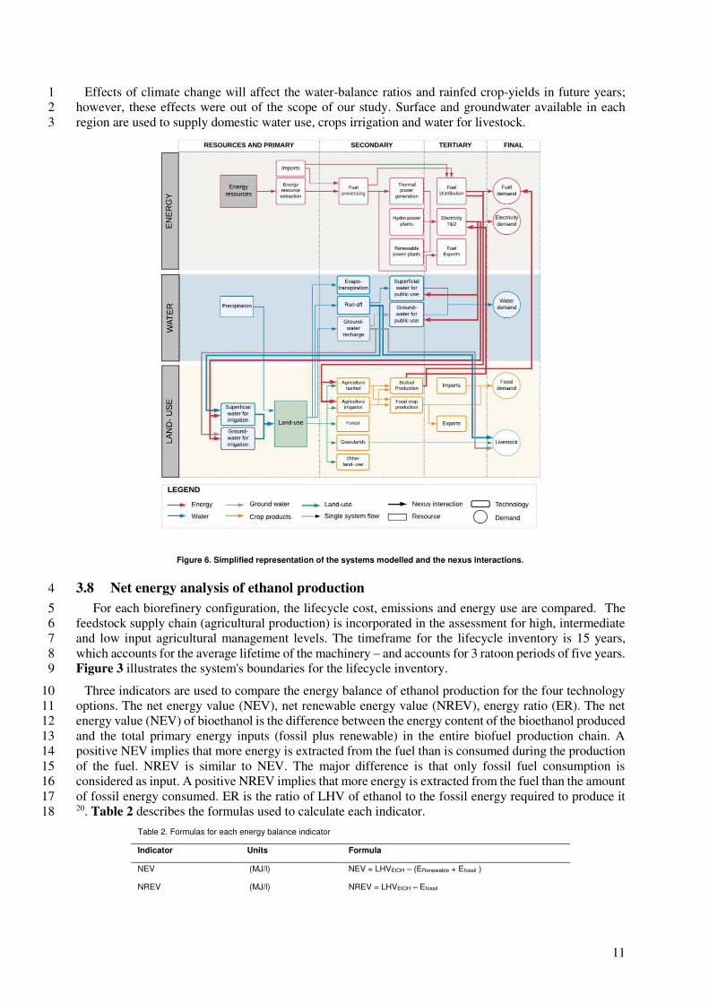
Figure 6 presents a simplified scheme of the model developed with the represented nexus interactions. 23 The main components of each system are represented in boxes, and the flows of energy/water/land 24 resources to secondary, tertiary and to final demands of commodity products are illustrated with arrows. 25 The interlinkages between land-use, water and energy systems are highlighted with thick arrows. 26 Although the main elements of our model are the agricultural production and biorefinery units, new 27 investments and operations of these units are influenced by nexus interactions with the water, energy and 28 land-use systems. 29

3.7.1 Interactions with the energy system 30

The energy system models the extraction and transformation of fossil and renewable resources to 31 generate electricity, diesel and gasoline. Section 9.9 in Supplementary Materials details the model 32 components for oil refinery and power generation. If domestic resources are not sufficient to meet the 33 domestic energy demands, the model can import these fuels at international market prices. From the 34 energy system, electricity is supplied to water pumping for residential demand, agricultural irrigation and 35 livestock. Investments in the power system affect the cost of electricity production, therefore affecting the 36 cost of agriculture production with irrigation. Electricity surplus generated by biorefineries is connected 37 to the national grid, therefore displacing gas-fired generation. Diesel is supplied to the land-use system to 38 supply machinery use, such as tractors, harvesters and mechanical planters. 39

3.7.2 Interactions with the water system 40

The water system was modelled using results from the WBB 74. The WBB model uses data from 1980 41 to 2016 to generate the water balances at basin-level (96 basins modelled). The water balance for each 42 region was calculated by overlaying the water inflows and outflows of the basins contained. The 43 components represented in our model are precipitation, evapotranspiration, groundwater recharge and 44 run-off water. Each component is introduced as a ratio of water to area, and it is specific for each land-45 cover type. Results of the hydrological model for the years 2013, 2014, 2015 and 2016 were introduced 46 directly while averages of the last ten years were used as constant values for the period 2017-2030. Section 47 9.9.2 in Supplementary Materials describes the water model more in detail. 48

11

Effects of climate change will affect the water-balance ratios and rainfed crop-yields in future years; 1 however, these effects were out of the scope of our study. Surface and groundwater available in each 2 region are used to supply domestic water use, crops irrigation and water for livestock. 3

Figure 6. Simplified representation of the systems modelled and the nexus interactions.

3.8 Net energy analysis of ethanol production 4

For each biorefinery configuration, the lifecycle cost, emissions and energy use are compared. The 5 feedstock supply chain (agricultural production) is incorporated in the assessment for high, intermediate 6 and low input agricultural management levels. The timeframe for the lifecycle inventory is 15 years, 7 which accounts for the average lifetime of the machinery – and accounts for 3 ratoon periods of five years. 8 Figure 3 illustrates the system's boundaries for the lifecycle inventory. 9

Three indicators are used to compare the energy balance of ethanol production for the four technology 10 options. The net energy value (NEV), net renewable energy value (NREV), energy ratio (ER). The net 11 energy value (NEV) of bioethanol is the difference between the energy content of the bioethanol produced 12 and the total primary energy inputs (fossil plus renewable) in the entire biofuel production chain. A 13 positive NEV implies that more energy is extracted from the fuel than is consumed during the production 14 of the fuel. NREV is similar to NEV. The major difference is that only fossil fuel consumption is 15 considered as input. A positive NREV implies that more energy is extracted from the fuel than the amount 16 of fossil energy consumed. ER is the ratio of LHV of ethanol to the fossil energy required to produce it 17 20. Table 2 describes the formulas used to calculate each indicator. 18

Table 2. Formulas for each energy balance indicator

Indicator Units Formula

NEV (MJ/l) NEV = LHVEtOH – (ERenewable + Efossil )

NREV (MJ/l) NREV = LHVEtOH – Efossil

12

ER (MJtot /MJfossil fuel ) ER = (EEtOH + Eelectricity surplus) / Efossil

3.9 Scenarios modelled 1

3.9.1 Sensitivity scenarios 2

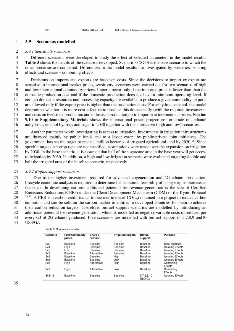
Different scenarios were developed to study the effect of selected parameters in the model results. 3 Table 3 shows the details of the scenarios developed. Scenario 0 (SC0) is the base scenario to which the 4 other scenarios are compared. Differences in the model results are investigated by scenarios isolating 5 effects and scenarios combining effects. 6

Decisions on imports and exports are based on costs. Since the decisions to import or export are 7 sensitive to international market prices, sensitivity scenarios were carried out for two scenarios of high 8 and low international commodity prices. Imports occur only if the imported price is lower than than the 9 domestic production cost and if the domestic production does not have a minimum operating level. If 10 enough domestic resources and processing capacity are available to produce a given commodity, exports 11 are allowed only if the export price is higher than the production costs. For anhydrous ethanol, the model 12 determines whether it is more cost-effective to produce this domestically (with the required investments 13 and costs on feedstock production and industrial production) or to import it at international prices. Section 14 9.10 in Supplementary Materials shows the international prices projections for crude oil, ethanol 15 anhydrous, ethanol hydrous and sugar to 2030 together with the alternative (high and low) scenarios. 16

Another parameter worth investigating is access to irrigation. Investments in irrigation infrastructures 17 are financed mainly by public funds and to a lesser extent by public-private joint initiatives. The 18 government has set the target to reach 1 million hectares of irrigated agricultural land by 2030 75. Since 19 specific targets per crop type are not specified, assumptions were made over the expansion on irrigation 20 by 2030. In the base scenario, it is assumed that half of the sugarcane area in the base year will get access 21 to irrigation by 2030. In addition, a high and low irrigation scenario were evaluated targeting double and 22 half the irrigated area of the baseline scenario, respectively. 23

3.9.2 Biofuel support scenarios 24

Due to the higher investment required for advanced cogeneration and 2G ethanol production, 25 lifecycle economic analysis is required to determine the economic feasibility of using surplus biomass as 26 feedstock. In developing nations, additional potential for revenue generation is the sale of Certified 27 Emissions Reductions (CERs) under the Clean Development Mechanism (CDM) of the Kyoto Protocol 28 76,77. A CER is a carbon credit (equal to one metric ton of CO2,eq) obtained in a project to reduce carbon 29 emissions and can be sold on the carbon market to entities in developed countries for them to achieve 30 their carbon reduction targets. Therefore, biofuel support scenarios are modelled by introducing an 31 additional potential for revenue generation, which is modelled as negative variable costs introduced per 32 every GJ of 2G ethanol produced. Five scenarios are modelled with biofuel support of 5,7,8,9 and10 33 US$/GJ. 34

Table 3. Scenarios modelled

Scenario Fuel/commodity prices

Energy demand

Irrigation targets Biofuel support

Purpose

Sc0 Baseline Baseline Baseline Baseline Base scenario Sc1 High Baseline Baseline Baseline Isolating Effects Sc2 Low Baseline Baseline Baseline Isolating Effects Sc3 Baseline Alternative Baseline Baseline Isolating Effects Sc4 Baseline Baseline High Baseline Isolating Effects Sc5 Baseline Baseline Low Baseline Isolating Effects Sc6 High Alternative High Baseline Combining

Effects Sc7 High Alternative Low Baseline Combining

Effects Sc8-12 Baseline Baseline Baseline 5,7,8,9,10

USD/GJ Isolating Effects

35

13

4 Results and discussion 1

4.1 Agricultural production 2

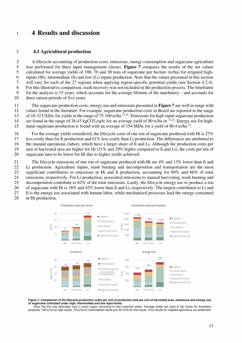
A lifecycle accounting of production costs, emissions, energy consumption and sugarcane agriculture 3 was performed for three input management classes. Figure 7 compares the results of the net values 4 calculated for average yields of 100, 70 and 30 tons of sugarcane per hectare (tc/ha) for irrigated high-5 inputs (Hi), intermediate (Ii) and low (Li) inputs production. Note that the values presented in this section 6 will vary for each of the 27 regions when applying region-specific potential yields (see Section 4.2.4). 7 For this illustrative comparison, trash recovery was not included in the production process. The timeframe 8 for the analysis is 15 years, which accounts for the average lifetime of the machinery – and accounts for 9 three ratoon periods of five years. 10

The sugarcane production costs, energy use and emissions presented in Figure 7 are well in range with 11 values found in the literature. For example, sugarcane production costs in Brazil are reported in the range 12 of 18-32 US$/tc for yields in the range of 75-100 tc/ha 13,34. Emissions for high-input sugarcane production 13 are found in the range of 38-43 kgCO2,eq/tc for an average yield of 80 tc/ha in 13,22. Energy use for high-14 input sugarcane production is found with an average of 154 MJ/tc for a yield of 86.4 tc/ha 22. 15

For the average yields considered, the lifecycle costs of one ton of sugarcane produced with Hi is 27% 16 less costly than for Ii production and 61% less costly than Li production. The differences are attributed to 17 the manual operations (labor), which have a larger share of Ii and Li. Although the production costs per 18 unit of harvested area are higher for Hi (21% and 29% higher compared to Ii and Li), the costs per ton of 19 sugarcane turn to be lower for Hi due to higher yields achieved. 20

The lifecycle emissions of one ton of sugarcane produced with Hi are 4% and 13% lower than Ii and 21 Li production. Agriculture inputs, trash burning and decomposition and transportation are the most 22 significant contributors to emissions in Hi and Ii production, accounting for 69% and 66% of total 23 emissions, respectively. For Li production, associated emissions to manual harvesting, trash burning and 24 decomposition contribute to 62% of the total emissions. Lastly, the lifecycle energy use to produce a ton 25 of sugarcane with Hi is 18% and 42% lower than Ii and Li, respectively. The largest contributor to Li and 26 Ii is the energy use associated with human labor, while mechanized processes lead the energy consumed 27 in Hi production. 28

Figure 7. Comparison of the lifecycle production costs per unit of production and per unit of harvested area, emissions and energy use of sugarcane cultivated under high, intermediate and low input levels.

- Note that the cost estimates vary in every region according to their potential yields. Average yields are used in the charts for illustrative purposes: 100 tc/ha for high-inputs, 70 tc/ha for intermediate inputs and 30 tc/ha for low-inputs. Only results for irrigated agriculture are presented.

22

30

56

-

15

30

45

60

High Intermediate Low

US

D/t

c

Production costs per tonne

Irrigation

Transportation

Harvesting

Agriculture inputs

Sugarcane farming

2 163

1 7831 668

-

500

1 000

1 500

2 000

2 500

High Intermediate Low

US

D/h

a

Production costs per hectare

Irrigation

Transportation

Harvesting

Agriculture inputs

Sugarcane farming

4648

53

-

15

30

45

60

High Intermediate Low

kgC

o2

,eq

/tc

Emissions

Irrigation

Field emissions

Trash burning and

decompositionTransportation

Harvesting

Agriculture inputs

Sugarcane farming

214

260

369

-

100

200

300

400

High Intermediate Low

MJ/

tc

Energy Use

Irrigation

Transportation

Harvesting

Agriculture inputs

Sugarcane farming

14

- Note that the charts do not show data for production with trash recovery. Additional costs of harvesting and transport are introduced together with reduced emissions estimated in 13.

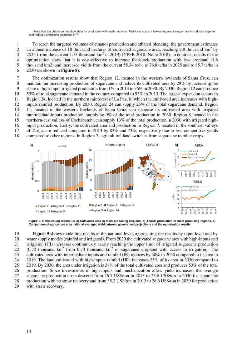
To reach the targeted volumes of ethanol production and ethanol blending, the government estimates 1 an annual increase of 18 thousand hectares of cultivated sugarcane area, reaching 2.8 thousand km2 by 2 2025 (from the current 1.73 thousand km2 in 2019) (YPFB 2018; Nolte 2018). In contrast, results of the 3 optimization show that it is cost-effective to increase feedstock production with less cropland (1.6 4 thousand km2) and increased yields from the current 55.34 tc/ha to 76.8 tc/ha in 2025 and to 85.7 tc/ha in 5 2030 (as shown in Figure 8). 6

The optimization results show that Region 12, located in the western lowlands of Santa Cruz, can 7 maintain an increasing production of sugarcane and reduce its cultivated area by 29% by increasing the 8 share of high-input irrigated production from 1% in 2013 to 56% in 2030. By 2030, Region 12 can produce 9 53% of total sugarcane demand in the country compared to 93% in 2013. The largest expansion occurs in 10 Region 24, located in the northern rainforest of La Paz, in which the cultivated area increases with high-11 inputs rainfed production. By 2030, Region 24 can supply 25% of the total sugarcane demand. Region 12 11, located in the western lowlands of Santa Cruz, can increase its cultivated area with irrigated 13 intermediate-inputs production, supplying 9% of the total production in 2030. Region 8 located in the 14 northern-east valleys of Cochabamba can supply 13% of the total production in 2030 with irrigated high-15 input production. Lastly, the cultivated area and production in Region 7, located in the southern valleys 16 of Tarija, are reduced compared to 2013 by 83% and 73%, respectively due to less competitive yields 17 compared to other regions. In Region 7, agricultural land switches from sugarcane to other crops. 18

Figure 8. Optimization results for a) Cultivated area in main producing Regions, b) Annual production of main producing regions, c) Comparison of agriculture area national averaged yield between government projections and the optimization results

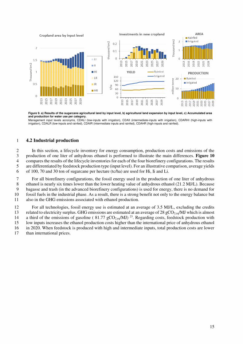
Figure 9 shows modelling results at the national level, aggregating the results by input level and by 19 water supply modes (rainfed and irrigated). From 2020 the cultivated sugarcane area with high-inputs and 20 irrigation (HI) increases continuously nearly reaching the upper limit of irrigated sugarcane production 21 (0.70 thousand km2 from 0.73 thousand km2 of sugarcane cropland with access to irrigation). The 22 cultivated area with intermediate inputs and rainfed (IR) reduces by 38% in 2030 compared to its area in 23 2019. The land cultivated with high-inputs rainfed (HR) increases 25% of its area in 2030 compared to 24 2019. By 2030, the area under irrigation is 38% of the total cultivated area and produces 53% of the total 25 production. Since investments in high-inputs and mechanization allow yield increases, the average 26 sugarcane production costs descend from 26.7 US$/ton in 2013 to 23.6 US$/ton in 2030 for sugarcane 27 production with no straw recovery and from 35.2 US$/ton in 2013 to 28.6 US$/ton in 2030 for production 28 with straw recovery. 29

15

Figure 9. a) Results of the sugarcane agricultural land by input level, b) agricultural land expansion by input level, c) Accumulated area and production for water use per category.

Management input levels acronyms, CDALI (low-inputs with irrigation), CDAII (intermediate-inputs with irrigation), CDARHI (high-inputs with irrigation), CDALR (low-inputs and rainfed), CDAIR (intermediate inputs and rainfed), CDAHR (high-inputs and rainfed).

4.2 Industrial production 1

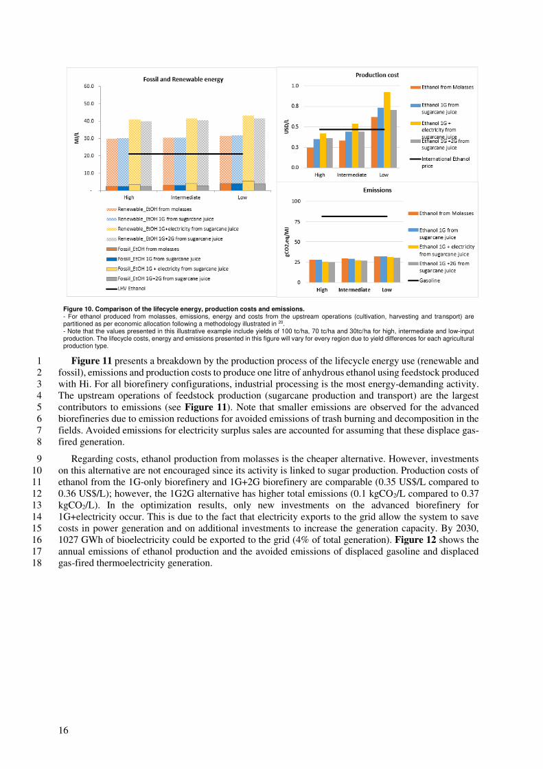
In this section, a lifecycle inventory for energy consumption, production costs and emissions of the 2 production of one liter of anhydrous ethanol is performed to illustrate the main differences. Figure 10 3 compares the results of the lifecycle inventories for each of the four biorefinery configurations. The results 4 are differentiated by feedstock production type (input level). For an illustrative comparison, average yields 5 of 100, 70 and 30 ton of sugarcane per hectare (tc/ha) are used for Hi, Ii and Li. 6

For all biorefinery configurations, the fossil energy used in the production of one liter of anhydrous 7 ethanol is nearly six times lower than the lower heating value of anhydrous ethanol (21.2 MJ/L). Because 8 bagasse and trash (in the advanced biorefinery configurations) is used for energy, there is no demand for 9 fossil fuels in the industrial phase. As a result, there is a strong benefit not only to the energy balance but 10 also in the GHG emissions associated with ethanol production. 11

For all technologies, fossil energy use is estimated at an average of 3.5 MJ/L, excluding the credits 12 related to electricity surplus. GHG emissions are estimated at an average of 28 gCO2,eq/MJ which is almost 13 a third of the emissions of gasoline ( 81.77 gCO2,eq/MJ) 23. Regarding costs, feedstock production with 14 low inputs increases the ethanol production costs higher than the international price of anhydrous ethanol 15 in 2020. When feedstock is produced with high and intermediate inputs, total production costs are lower 16 than international prices. 17

16

Figure 10. Comparison of the lifecycle energy, production costs and emissions. - For ethanol produced from molasses, emissions, energy and costs from the upstream operations (cultivation, harvesting and transport) are partitioned as per economic allocation following a methodology illustrated in 20. - Note that the values presented in this illustrative example include yields of 100 tc/ha, 70 tc/ha and 30tc/ha for high, intermediate and low-input production. The lifecycle costs, energy and emissions presented in this figure will vary for every region due to yield differences for each agricultural production type.

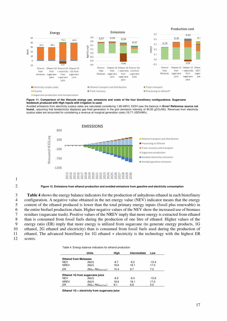
Figure 11 presents a breakdown by the production process of the lifecycle energy use (renewable and 1 fossil), emissions and production costs to produce one litre of anhydrous ethanol using feedstock produced 2 with Hi. For all biorefinery configurations, industrial processing is the most energy-demanding activity. 3 The upstream operations of feedstock production (sugarcane production and transport) are the largest 4 contributors to emissions (see Figure 11). Note that smaller emissions are observed for the advanced 5 biorefineries due to emission reductions for avoided emissions of trash burning and decomposition in the 6 fields. Avoided emissions for electricity surplus sales are accounted for assuming that these displace gas-7 fired generation. 8

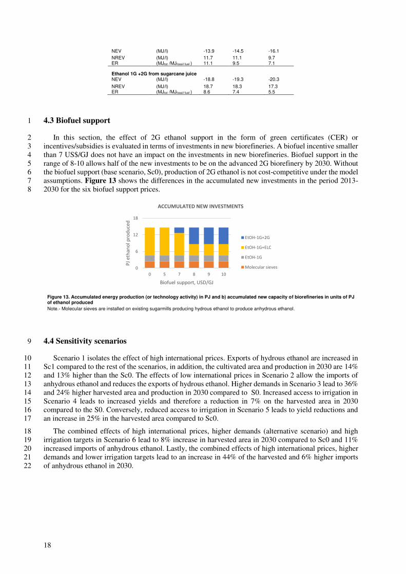
Regarding costs, ethanol production from molasses is the cheaper alternative. However, investments 9 on this alternative are not encouraged since its activity is linked to sugar production. Production costs of 10 ethanol from the 1G-only biorefinery and 1G+2G biorefinery are comparable (0.35 US$/L compared to 11 0.36 US$/L); however, the 1G2G alternative has higher total emissions (0.1 kgCO2/L compared to 0.37 12 kgCO2/L). In the optimization results, only new investments on the advanced biorefinery for 13 1G+electricity occur. This is due to the fact that electricity exports to the grid allow the system to save 14 costs in power generation and on additional investments to increase the generation capacity. By 2030, 15 1027 GWh of bioelectricity could be exported to the grid (4% of total generation). Figure 12 shows the 16 annual emissions of ethanol production and the avoided emissions of displaced gasoline and displaced 17 gas-fired thermoelectricity generation. 18

17

Figure 11. Comparison of the lifecycle energy use, emissions and costs of the four biorefinery configurations. Sugarcane feedstock produced with High inputs with irrigation is used.

Avoided emissions from electricity surplus sales are calculated considering 1.68 kWh/L EtOH (see the balance in Error! Reference source not found., assuming that bioelectricity displaces gas-fired generation in the grid (emission intensity of 90.93 gCO2/MJ). Revenues from electricity surplus sales are accounted for considering a revenue at marginal generation costs (16.71 USD/kWh).

1

Figure 12. Emissions from ethanol production and avoided emissions from gasoline and electricity consumption 2

Table 4 shows the energy balance indicators for the production of anhydrous ethanol in each biorefinery 3 configuration. A negative value obtained in the net energy value (NEV) indicator means that the energy 4 content of the ethanol produced is lower than the total primary energy inputs (fossil plus renewable) in 5 the entire biofuel production chain. Higher negative values of the NEV show the increased use of biomass 6 residues (sugarcane trash). Positive values of the NREV imply that more energy is extracted from ethanol 7 than is consumed from fossil fuels during the production of one litre of ethanol. Higher values of the 8 energy ratio (ER) imply that more energy is utilized from sugarcane (to generate energy products, 1G 9 ethanol, 2G ethanol and electricity) than is consumed from fossil fuels used during the production of 10 ethanol. The advanced biorefinery for 1G ethanol + electricity is the technology with the highest ER 11 scores. 12

Table 4. Energy balance indicators for ethanol production

Units High Intermediate Low

Ethanol from Molasses NEV (MJ/l) -8.7 -9.2 -10.4 NREV (MJ/l) 18.6 18.1 17.0

ER (MJtot /MJfossil fuel ) 10.4 9.7 7.0

Ethanol 1G from sugarcane juice NEV (MJ/l) -8.9 -9.4 -10.6

NREV (MJ/l) 18.6 18.1 17.0 ER (MJtot /MJfossil fuel ) 8.1 6.8 5.0

Ethanol 1G + electricity from sugarcane juice

Electricity surplus sales Ethanol transport and distribution Trash transport

Enzyme Trash recovery Processing to ethanol*

Sugarcane production and transportation

-1200

-700

-200

300

800

20

13

20

14

20

15

20

16

20

17

20

18

20

19

20

20

20

21

20

22

20

23

20

24

20

25

20

26

20

27

20

28

20

29

20

30

tho

usa

nd

tC

O2

,eq

EMISSIONS

Ethanol transport and distribution

Processing to Ethanol

Trash recovery and transport

Sugarcane production

Avoided electricity emissions

Avoided gasoline emissions

18

NEV (MJ/l) -13.9 -14.5 -16.1

NREV (MJ/l) 11.7 11.1 9.7 ER (MJtot /MJfossil fuel ) 11.1 9.5 7.1

Ethanol 1G +2G from sugarcane juice NEV (MJ/l) -18.8 -19.3 -20.3

NREV (MJ/l) 18.7 18.3 17.3 ER (MJtot /MJfossil fuel ) 8.6 7.4 5.5

4.3 Biofuel support 1

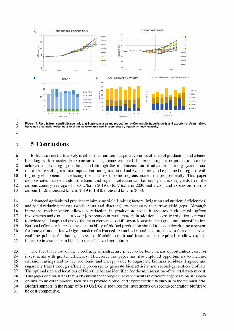
In this section, the effect of 2G ethanol support in the form of green certificates (CER) or 2 incentives/subsidies is evaluated in terms of investments in new biorefineries. A biofuel incentive smaller 3 than 7 US$/GJ does not have an impact on the investments in new biorefineries. Biofuel support in the 4 range of 8-10 allows half of the new investments to be on the advanced 2G biorefinery by 2030. Without 5 the biofuel support (base scenario, Sc0), production of 2G ethanol is not cost-competitive under the model 6 assumptions. Figure 13 shows the differences in the accumulated new investments in the period 2013-7 2030 for the six biofuel support prices. 8

Figure 13. Accumulated energy production (or technology activity) in PJ and b) accumulated new capacity of biorefineries in units of PJ of ethanol produced

Note.- Molecular sieves are installed on existing sugarmills producing hydrous ethanol to produce anhydrous ethanol.

4.4 Sensitivity scenarios 9

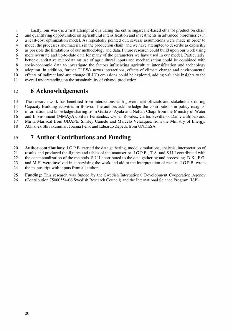
Scenario 1 isolates the effect of high international prices. Exports of hydrous ethanol are increased in 10 Sc1 compared to the rest of the scenarios, in addition, the cultivated area and production in 2030 are 14% 11 and 13% higher than the Sc0. The effects of low international prices in Scenario 2 allow the imports of 12 anhydrous ethanol and reduces the exports of hydrous ethanol. Higher demands in Scenario 3 lead to 36% 13 and 24% higher harvested area and production in 2030 compared to S0. Increased access to irrigation in 14 Scenario 4 leads to increased yields and therefore a reduction in 7% on the harvested area in 2030 15 compared to the S0. Conversely, reduced access to irrigation in Scenario 5 leads to yield reductions and 16 an increase in 25% in the harvested area compared to Sc0. 17

The combined effects of high international prices, higher demands (alternative scenario) and high 18 irrigation targets in Scenario 6 lead to 8% increase in harvested area in 2030 compared to Sc0 and 11% 19 increased imports of anhydrous ethanol. Lastly, the combined effects of high international prices, higher 20 demands and lower irrigation targets lead to an increase in 44% of the harvested and 6% higher imports 21 of anhydrous ethanol in 2030. 22

0

6

12

18

0 5 7 8 9 10

PJ

eth

an

ol

pro

du

ced

Biofuel support, USD/GJ

ACCUMULATED NEW INVESTMENTS

EtOH-1G+2G

EtOH-1G+ELC

EtOH-1G

Molecular sieves

19

1 Figure 14. Results from sensitivity scenarios. a) Sugarcane area and production. b) Commodity trade (imports and exports). c) Accumulated 2 harvested area (activity) by input level and accumulated new investments by input level (new capacity) 3

4

5 Conclusions 5

Bolivia can cost-effectively reach its medium-term targeted volumes of ethanol production and ethanol 6 blending with a moderate expansion of sugarcane cropland. Increased sugarcane production can be 7 achieved on existing agricultural land through the implementation of advanced farming systems and 8 increased use of agricultural inputs. Further agricultural land expansions can be planned in regions with 9 higher yield potentials, reducing the land use in other regions more than proportionally. This paper 10 demonstrates that demands for ethanol and sugar production can be met by increasing yields from the 11 current country-average of 55.3 tc/ha in 2019 to 85.7 tc/ha in 2030 and a cropland expansion from its 12 current 1.726 thousand km2 in 2019 to 1.840 thousand km2 in 2030. 13

Advanced agricultural practices minimizing yield-limiting factors (irrigation and nutrient deficiencies) 14 and yield-reducing factors (weds, pests and diseases) are necessary to narrow yield gaps. Although 15 increased mechanization allows a reduction in production costs, it requires high-capital upfront 16 investments and can lead to lower job creation in rural areas 13. In addition, access to irrigation is pivotal 17 to reduce yield gaps and one of the main elements to shift towards sustainable agriculture intensification. 18 National efforts to increase the sustainability of biofuel production should focus on developing a system 19 for innovation and knowledge transfer of advanced technologies and best practices to farmers 11. Also, 20 enabling policies facilitating access to affordable credit and insurance are required to allow capital-21 intensive investments in high-input mechanized agriculture. 22

The fact that most of the biorefinery infrastructure is yet to be built means opportunities exist for 23 investments with greater efficiency. Therefore, this paper has also explored opportunities to increase 24 emission savings and to add economic and energy value to sugarcane biomass residues (bagasse and 25 sugarcane trash) through efficient processes to generate bioelectricity and second-generation biofuels. 26 The optimal size and locations of biorefineries are identified for the minimization of the total system cost. 27 This paper demonstrates that with current technological advancements in efficient cogeneration, it is cost-28 optimal to invest in modern facilities to provide biofuel and export electricity surplus to the national grid. 29 Biofuel support in the range of 8-10 US$/GJ is required for investments on second-generation biofuel to 30 be cost-competitive. 31

20

Lastly, our work is a first attempt at evaluating the entire sugarcane-based ethanol production chain 1 and quantifying opportunities on agricultural intensification and investments in advanced biorefineries in 2 a least-cost optimization model. As repeatedly pointed out, several assumptions were made in order to 3 model the processes and materials in the production chain, and we have attempted to describe as explicitly 4 as possible the limitations of our methodology and data. Future research could build upon our work using 5 more accurate and up-to-date data for many of the parameters we have used in our model. Particularly, 6 better quantitative microdata on use of agricultural inputs and mechanization could be combined with 7 socio-economic data to investigate the factors influencing agriculture intensification and technology 8 adoption. In addition, further CLEWs nexus interactions, effects of climate change and environmental 9 effects of indirect land-use change (iLUC) emissions could be explored, adding valuable insights to the 10 overall understanding on the sustainability of ethanol production. 11

6 Acknowledgements 12

The research work has benefited from interactions with government officials and stakeholders during 13 Capacity Building activities in Bolivia. The authors acknowledge the contributions in policy insights, 14 information and knowledge-sharing from Gustavo Ayala and Neftali Chapi from the Ministry of Water 15 and Environment (MMAyA), Silvia Fernández, Osmar Rosales, Carlos Sevillano, Daniela Bilbao and 16 Mirna Mariscal from UDAPE, Shirley Canedo and Marcelo Velazquez from the Ministry of Energy, 17 Abhishek Shivakummar, Joanna Félix and Eduardo Zepeda from UNDESA. 18

7 Author Contributions and Funding 19

Author contributions: J.G.P.B. carried the data gathering, model simulations, analysis, interpretation of 20 results and produced the figures and tables of the manuscript. J.G.P.B., T.A. and S.U.J contributed with 21 the conceptualization of the methods. S.U.J contributed to the data gathering and processing. D.K., F.G. 22 and M.H. were involved in supervising the work and aid to the interpretation of results. J.G.P.B. wrote 23 the manuscript with inputs from all authors. 24

Funding: This research was funded by the Swedish International Development Cooperation Agency 25 (Contribution 75000554-06 Swedish Research Council) and the International Science Program (ISP). 26

21

8 References

1. Koçar, G. & Civaş, N. An overview of biofuels from energy crops: Current status and future prospects. Renewable and Sustainable Energy Reviews 28, 900–916 (2013).

2. Scarlat, N. & Dallemand, J. F. Recent developments of biofuels/bioenergy sustainability certification: A global overview. Energy Policy 39, 1630–1646 (2011).

3. de Oliveira Bordonal, R. et al. Sustainability of sugarcane production in Brazil. A review. Agron.

Sustain. Dev. 38, 13 (2018).

4. Dahman, Y., Syed, K., Begum, S., Roy, P. & Mohtasebi, B. Biofuels: Their characteristics and analysis. in Biomass, Biopolymer-Based Materials, and Bioenergy: Construction, Biomedical, and

other Industrial Applications 277–325 (Elsevier, 2019). doi:10.1016/B978-0-08-102426-3.00014-X

5. Nanda, S., Rana, R., Sarangi, P. K., Dalai, A. K. & Kozinski, J. A. A broad introduction to first-, second-, and third-generation biofuels. in Recent Advancements in Biofuels and Bioenergy

Utilization 1–25 (Springer Singapore, 2018). doi:10.1007/978-981-13-1307-3_1

6. International Energy Agency. World Energy Outlook 2019. (OECD, 2019). doi:10.1787/caf32f3b-en

7. OECD-FAO. Agricultural Outlook 2019-2028. Chapter 9. Biofuels. in (2019). doi:10.1787/agr-outl-data-en

8. Goldemberg, J. The Brazilian biofuels industry. Biotechnology for Biofuels 1, 6 (2008).

9. Van-den-Berg, M. & Singels, A. Modelling and monitoring for strategic yield gap diagnosis in the South African sugar belt. F. Crop. Res. 143, 143–150 (2013).

10. Mueller, N. D. et al. Closing yield gaps through nutrient and water management. Nature 490, 254–257 (2012).

11. van Dijk, M. et al. Disentangling agronomic and economic yield gaps: An integrated framework and application. Agric. Syst. 154, 90–99 (2017).

12. Van-Wart, J. et al. Use of agro-climatic zones to upscale simulated crop yield potential. F. Crop.

Res. 143, 44–55 (2013).

13. Cardoso, T. et al. Economic, environmental, and social impacts of different sugarcane production systems. Biofuels, Bioprod. Biorefining 12, 68–82 (2018).

14. Dias, M. O. S. et al. Biorefineries for the production of first and second generation ethanol and electricity from sugarcane. Appl. Energy 109, 72–78 (2013).

15. Khatiwada, D., Leduc, S., Silveira, S. & McCallum, I. Optimizing ethanol and bioelectricity production in sugarcane biorefineries in Brazil. Renew. Energy 85, 371–386 (2016).

16. Dias, M. O. S. et al. Improving bioethanol production from sugarcane: Evaluation of distillation, thermal integration and cogeneration systems. Energy 36, 3691–3703 (2011).

17. Dourado Hernandes, T., Bof Bufon, V. & Seabra, J. Water footprint of biofuels in Brazil : (2013). doi:10.1002/bbb

18. Vale Scarpare, F. et al. Sugarcane water footprint under different management practices in ^ / Jacar e watershed assessment Brazil : Tiet e. 112, 4576–4584 (2016).

19. Haro, M. E., Navarro, I., Thompson, R. & Jimenez, B. Estimation of the water footprint of sugarcane in Mexico : is ethanol production an environmentally feasible fuel option ? María Eugenia Haro , Ines Navarro , Ralph Thompson and Blanca Jimenez. J. Water Clim. Chang. 05, 70–80 (2014).

22

20. Khatiwada, D. & Silveira, S. Scenarios for bioethanol production in Indonesia: How can we meet mandatory blending targets? Energy 119, 351–361 (2017).

21. Khatiwada, D., Venkata, B., Silveira, S. & Johnson, F. Energy and GHG balances of ethanol production from cane molasses in Indonesia. Appl. Energy 164, 756–768 (2016).

22. Seabra, J., Macedo, I., Chum, H., Faroni, C. & Sarto, C. Life cycle assessment of Brazilian sugarcane products : GHG emissions and energy use. Biofuels, Bioproducs and Biorefining. 519–532 (2011). doi:10.1002/bbb

23. Macedo, I. C., Seabra, J. E. A. & Silva, J. E. A. R. Green house gases emissions in the production and use of ethanol from sugarcane in Brazil: The 2005/2006 averages and a prediction for 2020. Biomass and Bioenergy 32, 582–595 (2008).

24. van Ittersum, M. et al. Yield gap analysis with local to global relevance—A review. F. Crop. Res. 143, 4–17 (2013).

25. van Ittersum, M. & Rabbinge, R. Concepts in production ecology for analysis and quantification of agricultural input-output combinations. F. Crop. Res. 52, 197–208 (1997).

26. Van-Loon, J. et al. Scaling agricultural mechanization services in smallholder farming systems: Case studies from sub-Saharan Africa, South Asia, and Latin America. Agric. Syst. 180, 102792 (2020).

27. Yadav, R. N. S., Yadav, S. & Tejra, R. K. Labour Saving and Cost Reduction Machinery for Sugarcane Cultivation. Sugar Tech 5, 7–10 (2003).

28. Verma, S. R. Impact of Agricultural Mechanization on Production , Productivity , Cropping Intensity Income Generation and Employment of Labour. in Status of Farm Mechanization in

India (ed. Indian Agri. Stat. Research Indian Agri. Stat. Research Institute) 133–153 (Indian Council of Agricultural Research, 2006).

29. Dias, M. O. S. et al. Improving second generation ethanol production through optimization of first generation production process from sugarcane. Energy 43, 246–252 (2012).

30. Birru, E., Erlich, C. & Martin, A. Energy performance comparisons and enhancements in the sugar cane industry. Biomass Convers. Biorefinery 9, 267–282 (2019).

31. Birru, E. D. Process Utility Performance Evaluation and Enhancements in the Traditional Sugar

Cane Industry. (2019).

32. Deshmukh, R., Jacobson, A., Chamberlin, C. & Kammen, D. Thermal gasification or direct combustion? Comparison of advanced cogeneration systems inthe sugarcane industry. Biomass

and Bioenergy 55, 163–174 (2013).

33. ISO. Cogeneration-opportunities in the world sugar industry. (2009).

34. Dias, M. O. S. et al. Second generation ethanol in Brazil: Can it compete with electricity production? Bioresour. Technol. 102, 8964–8971 (2011).

35. Mbohwa, C. Bagasse energy cogeneration potential in the Zimbabwean sugar industry. 28, 191–204 (2003).

36. Nolte, G. E. USDA Foreign Agricultural Service. Global Agricultural Information Network.

Bolivia Enters Ethanol Era. (2018).

37. YPFB. Bolivia ingresa a la era del biocombustible. (2018). Available at: https://www.ypfb.gob.bo/en/medio-ambiente/14-noticias/841-bolivia-ingresa-a-la-era-del-biocombustible-y-ypfb-dejará-de-importar-80-millones-de-litros-de-gasolina-2.html. (Accessed: 23rd May 2020)

38. Instituto Nacional de Estadísticas. Encuesta Nacional Agropecuaria. Superficie cultivada,

producción y rendimiento. (2019).

39. Lobell, D. B., Cassman, K. G. & Field, C. B. Crop Yield Gaps: Their Importance, Magnitudes,

23

and Causes. Annu. Rev. Environ. Resour. 34, 179–204 (2009).

40. FAO. FAOSTAT. (2018). Available at: http://www.fao.org/faostat/en/#rankings/countries_by_commodity. (Accessed: 16th November 2018)

41. Instituto Nacional de Estadistica, I. Censo Agropecuario 2013 Bolivia. (2015).

42. Cruz, C. H. B., Souza, G. M. & Cortez, L. A. B. Biofuels for Transport. 215–244 (2014). doi:10.1016/B978-0-08-099424-6.00011-9

43. Howells, M. et al. OSeMOSYS: The Open Source Energy Modeling System. Energy Policy 39, 5850–5870 (2011).

44. Welsch, M. et al. Adding value with CLEWS - Modelling the energy system and its interdependencies for Mauritius. Appl. Energy 113, 1434–1445 (2014).

45. Pereira-Ramos, E. et al. The Climate Land Energy Water systems (CLEWs) Framework: A retrospective of activities and advances to 2019 - In Press. Environ. Res. Lett. (2020).

46. Ministerio de Medio Ambiente y Agua (MMAyA). Balance Hídrico Superficial de Bolivia 1980-

81- 2015/16. (2017).

47. Ministerio del Agua. Plan Nacional de Desarrollo del Riego 2007-2011. (2007).

48. Odum & T, H. Systems ecology; An introduction. (1983).

49. Nguyen, T. L. T., Gheewala, S. H. & Garivait, S. Full chain energy analysis of fuel ethanol from cassava in Thailand. Environ. Sci. Technol. 41, 4135–4142 (2007).

50. Nguyen, T. L. T. & Gheewala, S. H. Life cycle assessment of fuel ethanol from cane molasses in Thailand. Int. J. Life Cycle Assess. 13, 301–311 (2008).

51. Khatiwada, D. & Silveira, S. Greenhouse gas balances of molasses based ethanol in Nepal. J.

Clean. Prod. 19, 1471–1485 (2011).

52. Khatiwada, D. & Silveira, S. Net energy balance of molasses based ethanol: The case of Nepal. Renew. Sustain. Energy Rev. 13, 2515–2524 (2009).

53. Kahil, T. et al. A Continental-Scale Hydroeconomic Model for Integrating Water-Energy-Land Nexus Solutions. Water Resour. Res. 54, 7511–7533 (2018).

54. Observatorio Agroambiental y Productivo & Viceministerio de Desarrollo Rural y Agropecuario. Agricultural production costs per crop for mechanized, semi-mechanized and traditional production systems in departments of Bolivia. (2014). Available at: http://www.observatorioagro.gob.bo/index.php?variable=19. (Accessed: 22nd September 2020)

55. Bernués, A. & Herrero, M. Farm intensification and drivers of technology adoption in mixed dairy-crop systems in Santa Cruz, Bolivia. Spanish J. Agric. Res. 6, 279–293 (2008).

56. MDRyT. Compendio Agropecuario 2012 Observatorio Agroambiental y Productivo. (2012).

57. Cuentas, L. Producción y Política Azucarera. Scielo. Fides Ratio- Rev. Difusión Cult. y científica

la Univ. La Salle en Boliv. 5, (2012).

58. Fischer, G. et al. Global Agro-ecological Zones (GAEZ v3.0)- Model Documentation. (2012).

59. Allen, R. G., Pereira, L. S., Raes, D. & Smith, M. Crop evapotranspiration - Guidelines for computing crop water requirements - FAO Irrigation and drainage paper 56. in 1–15 (1998).

60. Yates, D., Sieber, J., Purkey, D. & Huber-Lee, A. WEAP21—A demand-, priority-, and preference-driven water planning model: part 1: model characteristics. Water Int. 30, 487–500 (2005).

61. Maidment, D. R. Handbook of hydrology (Vol.1). (McGraw-Hill, 1993).

62. Perez, R. Feeding pigs in the tropics. (1997).

24

63. Khatiwada, D., Seabra, J., Silveira, S. & Walter, A. Power generation from sugarcane biomass e A complementary option to hydroelectricity in Nepal and Brazil. Energy 48, 241–254 (2012).

64. Hassuani, S., Leal, M. & Macedo, I. Biomass Power Generation. Sugar Cane Bagasse and Trash. UNDP-UN and Centro de Tecnologia Canavieira-CTC (2005).

65. Cardoso, T. F. et al. Biomass and Bioenergy. A vertical integration simpli fi ed model for straw recovery as feedstock in sugarcane biorefineries. 81, 216–223 (2015).

66. World Energy Council- Bioenergy. World Energy Resources Bioenergy 2016. (2017).

67. UNAGRO. Memoria Institucional Unagro 2016-2018. (2019).

68. EASBA. Memoria Institucional Empresa Azucarera San Buenaventura. (2018).

69. IAGSA. Memoria Anual Ingenio Azucarero Guabira S.A. (2018).

70. Aguai. Memoria Institucional Ingenio Sucroalcoholero Aguai. (2018).

71. Southgate, D. The Causes of Land Degradation along ‘Spontaneously’ Expanding Agricultural Frontiers in the Third World. Land Econ. 66, 93–101 (1990).

72. Barbier, E. B. & Hochard, J. P. Land degradation and poverty. Nat. Sustain. 1, 623–631 (2018).

73. OECD-FAO. Agricultural Outlook 2017-2026. Commodity Snapshots. (2017). Available at: http://www.fao.org/3/a-BT092e.pdf.

74. Ministerio de Hidrocarburos. Balance Energético Nacional 2006-2018. (2019).

75. Estado Plurinacional de Bolivia. Intended Nationally determined contribution from the

Plurinational State of Bolivia,. (2015).

76. Flamos, A. et al. Bioenergy Options in the Industrialized and Developing World and Opportunities for the Clean Development Mechanism DEVELOPING WORLD AND OPPORTUNITIES FOR THE CLEAN DEVELOPMENT MECHANISM. 5075, (2010).

77. Mcnish, T., Jacobson, A., Kammen, D., Gopal, A. & Deshmukh, R. Sweet carbon : An analysis of sugar industry carbon market opportunities under the clean development mechanism. Energy

Policy 37, 5459–5468 (2009).

25

1

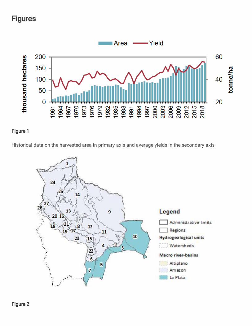
Figures

Figure 1

Historical data on the harvested area in primary axis and average yields in the secondary axis

Figure 2

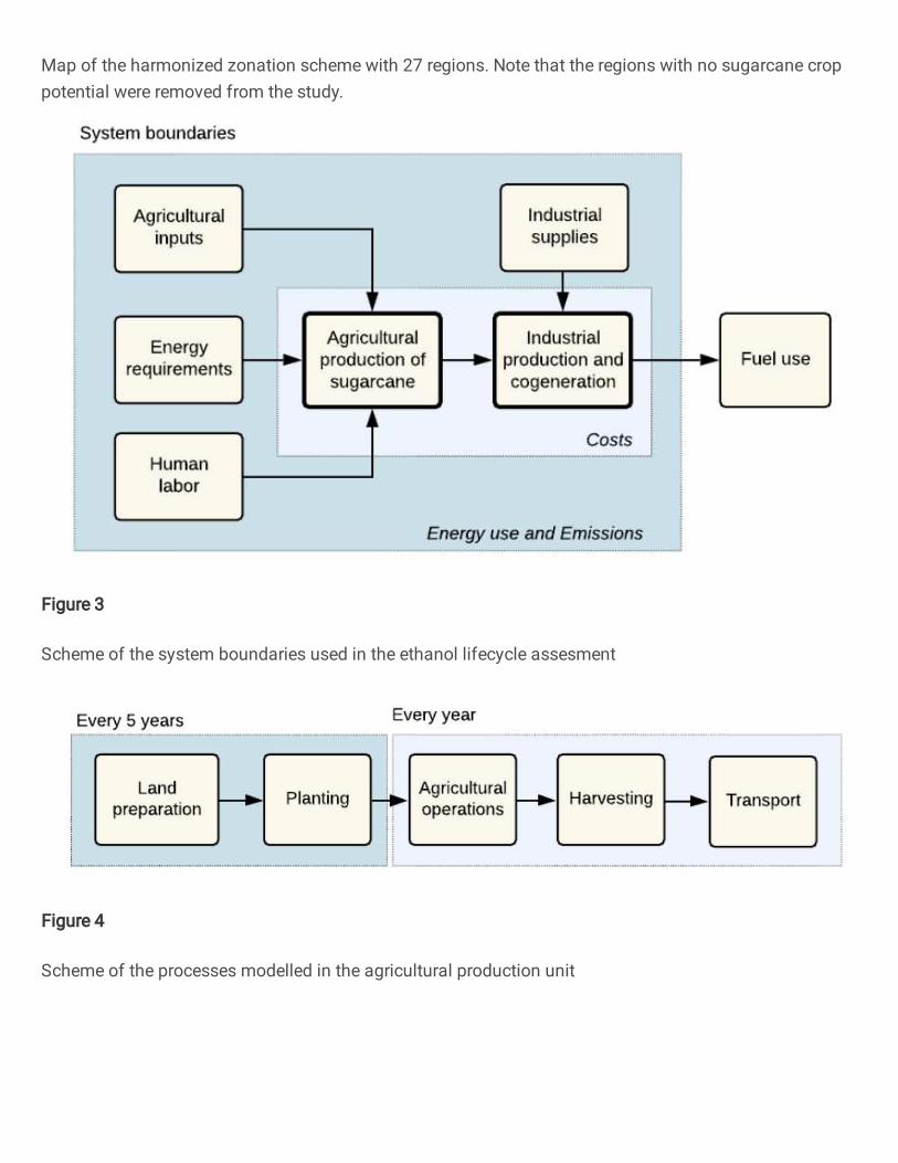
Map of the harmonized zonation scheme with 27 regions. Note that the regions with no sugarcane croppotential were removed from the study.

Figure 3

Scheme of the system boundaries used in the ethanol lifecycle assesment

Figure 4

Scheme of the processes modelled in the agricultural production unit

Figure 5

Biore�nery technological options. a) Biore�nery for 1G ethanol production using sugarcane molasses,conventional CHP plant (no sugarcane trash recovery), b) Biore�nery for 1G ethanol production usingsugarcane juice, conventional CHP plant (no sugarcane trash recovery), c) Biore�nery for 1G ethanolproduction with e�cient CHP and export of surplus electricity generation (50% of sugarcane trashrecovery), d) Biore�nery for 1G and 2G ethanol production with e�cient CHP (50% of sugarcane trashrecovery). Further details on the conversion chain are detailed in Section Error! Reference source notfound. in Supplementary Materials

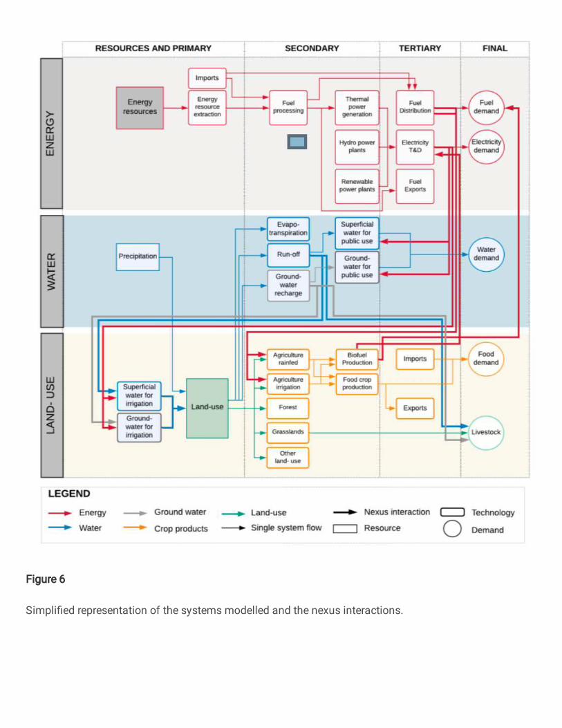
Figure 6

Simpli�ed representation of the systems modelled and the nexus interactions.

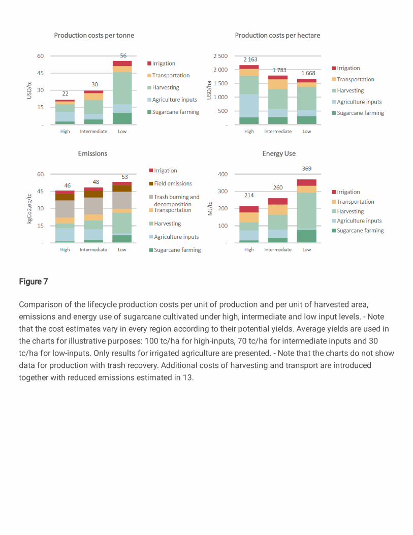
Figure 7

Comparison of the lifecycle production costs per unit of production and per unit of harvested area,emissions and energy use of sugarcane cultivated under high, intermediate and low input levels. - Notethat the cost estimates vary in every region according to their potential yields. Average yields are used inthe charts for illustrative purposes: 100 tc/ha for high-inputs, 70 tc/ha for intermediate inputs and 30tc/ha for low-inputs. Only results for irrigated agriculture are presented. - Note that the charts do not showdata for production with trash recovery. Additional costs of harvesting and transport are introducedtogether with reduced emissions estimated in 13.

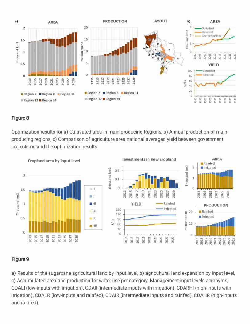
Figure 8

Optimization results for a) Cultivated area in main producing Regions, b) Annual production of mainproducing regions, c) Comparison of agriculture area national averaged yield between governmentprojections and the optimization results

Figure 9

a) Results of the sugarcane agricultural land by input level, b) agricultural land expansion by input level,c) Accumulated area and production for water use per category. Management input levels acronyms,CDALI (low-inputs with irrigation), CDAII (intermediate-inputs with irrigation), CDARHI (high-inputs withirrigation), CDALR (low-inputs and rainfed), CDAIR (intermediate inputs and rainfed), CDAHR (high-inputsand rainfed).

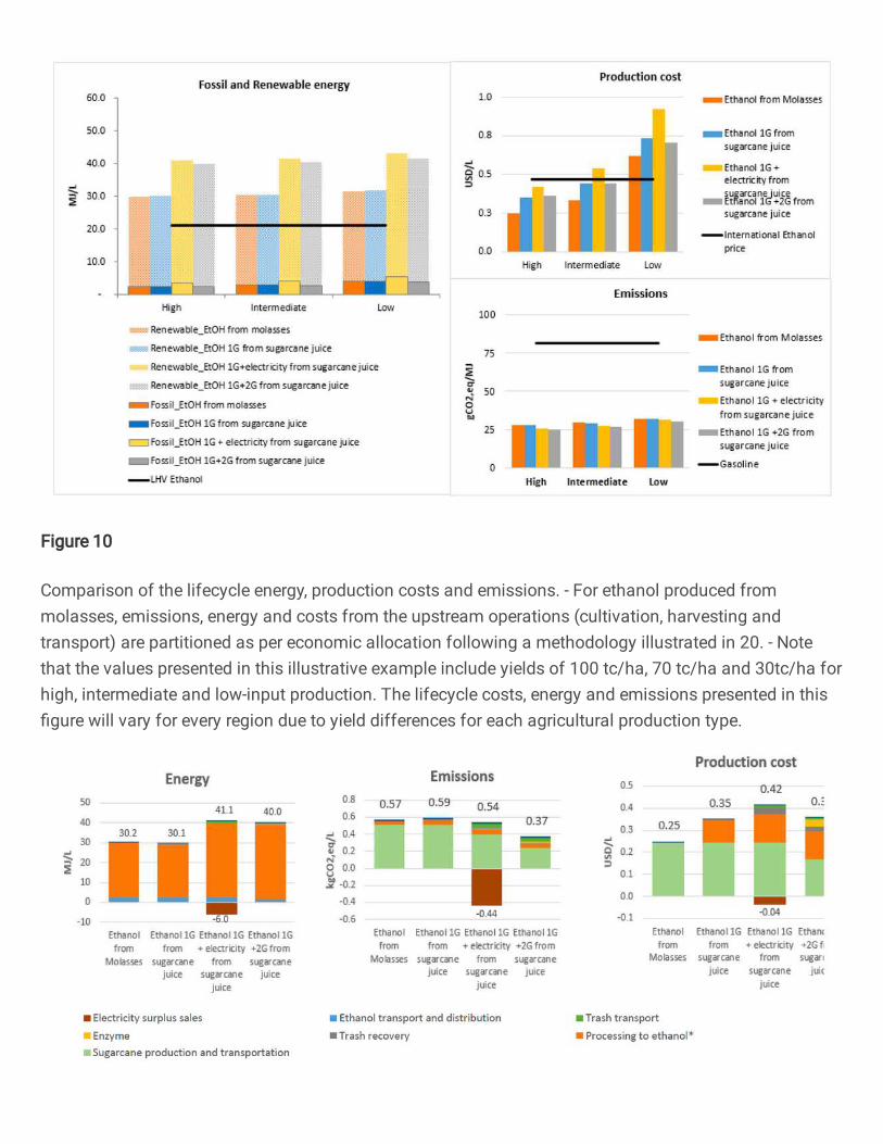
Figure 10

Comparison of the lifecycle energy, production costs and emissions. - For ethanol produced frommolasses, emissions, energy and costs from the upstream operations (cultivation, harvesting andtransport) are partitioned as per economic allocation following a methodology illustrated in 20. - Notethat the values presented in this illustrative example include yields of 100 tc/ha, 70 tc/ha and 30tc/ha forhigh, intermediate and low-input production. The lifecycle costs, energy and emissions presented in this�gure will vary for every region due to yield differences for each agricultural production type.

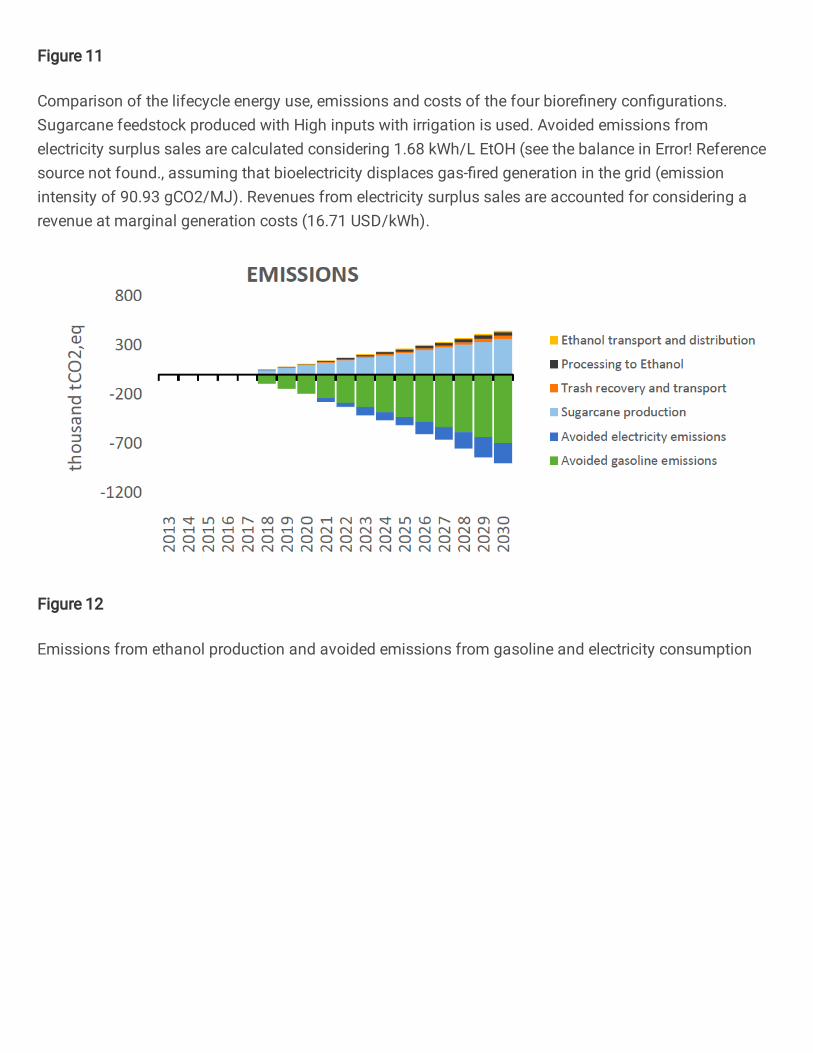
Figure 11

Comparison of the lifecycle energy use, emissions and costs of the four biore�nery con�gurations.Sugarcane feedstock produced with High inputs with irrigation is used. Avoided emissions fromelectricity surplus sales are calculated considering 1.68 kWh/L EtOH (see the balance in Error! Referencesource not found., assuming that bioelectricity displaces gas-�red generation in the grid (emissionintensity of 90.93 gCO2/MJ). Revenues from electricity surplus sales are accounted for considering arevenue at marginal generation costs (16.71 USD/kWh).

Figure 12

Emissions from ethanol production and avoided emissions from gasoline and electricity consumption

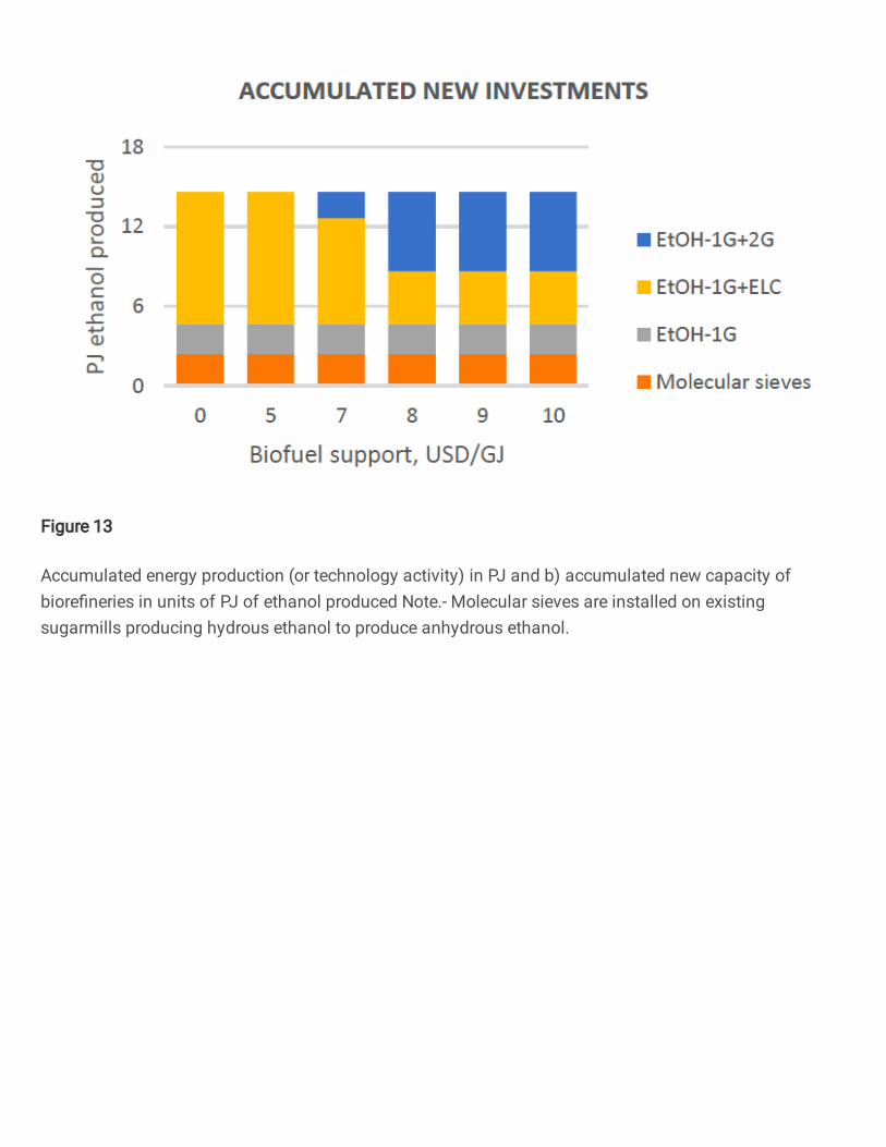
Figure 13

Accumulated energy production (or technology activity) in PJ and b) accumulated new capacity ofbiore�neries in units of PJ of ethanol produced Note.- Molecular sieves are installed on existingsugarmills producing hydrous ethanol to produce anhydrous ethanol.

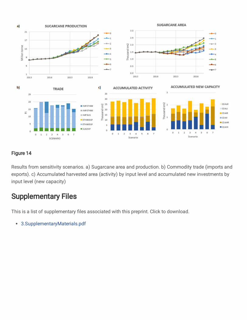
Figure 14

Results from sensitivity scenarios. a) Sugarcane area and production. b) Commodity trade (imports andexports). c) Accumulated harvested area (activity) by input level and accumulated new investments byinput level (new capacity)

Supplementary Files

This is a list of supplementary �les associated with this preprint. Click to download.

3.SupplementaryMaterials.pdf