Integrals and the Haar Measure - Project Euclid

CHAPTER 1

Integrals and the Haar Measure

In this and the next chapter, background material on integration, topological groups and group actions is presented. The concrete examples described below provide a direct connection between the rather abstract theory of Haar measure and its application to situations which are relevan't in statistical applications.

1.1. Integrals and measures. Our purpose in this section is to describe the connection between two different approaches to integration theory. The measure theory approach is commonly used in probability theory and so is familiar to most of us. However, the algebraic or linear functional approach is not so familiar. A good reference for the details of both approaches is Segal and Kunze (1978). A brief description of the linear functional approach and its relationship to the measure theory approach follows.

Let X be a locally compact topological space (Hausdorff) for which the topology has a countable base. That is, X is a topological space such that:

(i) The topology is Hausdorff. (ii) Each point of X has a compact neighborhood.

(iii) The topology has a countable base.

Throughout these notes, the word "space" refers to a topological space X satisfying (i), (ii) and (iii). In virtually all of our examples, X is an open or closed subset of a finite dimensional vector space (with the usual Euclidean topology) so that X with its inherited topology is a space.

In many discussions of integration on locally compact spaces, (iii) is not assumed. However, when (iii) does hold the a-algebra generated by the open sets (the Borel a-algebra) and the a-algebra generated by the compact sets (the Baire a-algebra) are identical. This circumstance simplifies the discussion somewhat and from our point of view is not a serious restriction of generality. The a-algebra associated with the space X is the Borel a-algebra = Baire a-algebra.

1

2 INTEGRALS AND THE HAAR MEASUHE

Given a space X, let K(X) be the set of all continuous real valued functions f defined on X which have compact support. Thus if f E K(X), there is a compact set C c X (which may vary from one f to another) such that f(x) = 0 if x $. C. For / 1, / 2 E K(X) and a 1, a 2 E R, it is clear that a1 / 1 + a 2 / 2 E K(X) so that K (X) is a real vector space.

DEFINITION 1.1. A real valued function J defined on K (X) which satisfies

(i) J(a1 / 1 + az/2 ) = a 1J(f1) + a 2J(f2 ) for /1, / 2 E K(X) and a 1, a 2 E R, (ii) J( f) ~ 0 whenever f E K(X) and f is nonnegative,

(iii) J( f) > 0 for some f E K(X)

is called an integral.

An integral J is a linear function defined on the vector space K (X) which maps nonnegative functions into nonnegative numbers. Assumption (iii) is to rule out the trivial case J = 0. Examples of integrals are easily constructed using Lebesgue measure when the space X is a subset of n dimensional Euclidean space Rn.

EXAMPLE 1.1. Assume X<;;; Rn with its inherited topology is a space and let dx denote Lebesgue measure restricted to X. If

1 dx > 0, X

define J on K (X) by

J(f ) = fx f (X) dx.

Because the Lebesgue measure of compact sets is finite, J( f ) is a well defined finite number for f E K(X). That J is an integral follows easily. However, care must be taken in some cases. For example, take X= ( -1, 1) and define a measure JL on the Borel sets of X using the function

go( X) = { ~~~ ' X =!= 0,

0, X= 0

via the equation

JL(B) = Jg0(x)dx. B

Then JL is a well defined a-finite measure on X but JL does not define an integral Vla

f --7 jt(x)JL(dx)

because there are functions in K (X) for which

jf(x)JL(dx) = +oo.

1.2. TOPOLOGICAL GROUPS 3

Of course, the problem arises because p. assigns measure + oo to some of the compact sets in X. D

In order to describe the relationship between integrals (as they are defined above) and measures, Example 1.1 shows the same sort of restriction has to be made. Here is the appropriate definition which facilitates the identification of integrals with measures and vice versa.

DEFINITION 1.2. On a space X, a measure p. defined on the Borel subsets of X is a Radon measure if p.( C) < + oo for all compact sets C s X and f.L of= 0.

THEOREM 1.1. Given an integral J defined on K(X), there is a unique Radon measure p. such that

(1.1) J(f) = jt(x)p.(dx), f E K(X).

Conversely, a Radon measure p. ¢ 0 defines an integral via (1.1).

The representation (1.1) sets up a one-to-one correspondence between integrals and Radon measures. In these notes, both representations are used with the choice being dictated by notational convenience and taste. Equation (1.1) allows the definition of an integral J to be extended to the class of functions which are p.-integrable. That is, if f is Borel-measurable and if

jl f(x)lp.(dx) < +oo,

then the right-hand side of (1.1) is well defined and so J( f) is defined via (1.1). In what follows, all integrals are automatically extended to the clas..'l of Borelmeasurable and p.-integrable functions.

1.2. Topological groups. A group is a nonempty set G together with a binary operation o such that the following conditions hold:

(i) g 1, g 2 E G implies g1 o g2 E G. (ii) (g1 o g2) o ga = g1 o (g2 o ga) for g1, g2, g3 E G.

(iii) There exists an element e E G such that e o g = g o e = g for g E G. (iv) For each g E G, there exists a unique element g- 1 E G such that

gog- 1 = g-1 o g = e.

The element e E G is called the identity and g- 1 is called the inverse of g. It is customary to suppress the symbol o when composing group elements. In this case, (ii) would be written (g1g 2)g3 = g1(g2g3 ). This custom is observed in what follows.

Now, assume that G is a group and that G is also a space as defined in Section 1.1. When the group operations fit together with the topology (i.e., are continuous), then G is a topological group. Here is the formal definition.

4 INTEGRALS AND THE HAAR MEASUHE

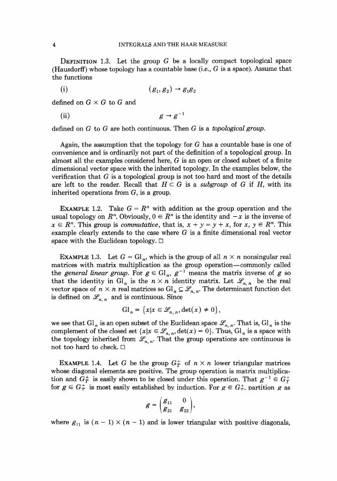
DEFINITION 1.3. Let the group G be a locally compact topological space (Hausdorff) whose topology has a countable base (i.e., G is a space). Assume that the functions

(i)

defined on G X G to G and

(ii)

defined on G to G are both continuous. Then G is a topological group.

Again, the assumption that the topology for G has a countable base is one of convenience and is ordinarily not part of the definition of a topological group. In almost all the examples considered here, G is an open or closed subset of a finite dimensional vector space with the inherited topology. In the examples below, the verification that G is a topological group is not too hard and most of the details are left to the reader. Recall that H c G is a subgroup of G if H, with its inherited operations from G, is a group.

EXAMPLE 1.2. Take G = Rn with addition as the group operation and the usual topology on Rn. Obviously, 0 ERn is the identity and -x is the inverse of x E Rn. This group is commutative, that is, x + y = y + x, for x, y E Rn. This example clearly extends to the case where G is a finite dimensional real vector space with the Euclidean topology. D

EXAMPLE 1.3. Let G = Gln, which is the group of all n X n nonsingular real matrices with matrix multiplication as the group operation-commonly called the general linear group. ForgE Gln, g- 1 means the matrix inverse of g so that the identity in Gln is the n X n identity matrix. Let .!l'n n be the real vector space of n X n real matrices so Gln ~ .!l'n n· The determina~t function det is defined on .!l'n n and is continuous. Since '

Gln = {xlx Efi>n,n,det(x) =fo 0},

we see that Gln is an open subset of the Euclidean space fi>n, n· That is, Gln is the complement of the closed set {xlx E fi>n, n• det(x) = 0}. Thus, Gln is a space with the topology inherited from fi>n, n· That the group operations are continuous is not too hard to check. D

EXAMPLE 1.4. Let G be the group G;J, of n X n lower triangular matrices whose diagonal elements are positive. The group operation is matrix multiplication and G;J, is easily shown to be closed under this operation. That g- 1 E G;J, for g E G~ is most easily established by induction. For ~ E G;f., partition p as

g = (;~~ g~J. where g 11 is (n- 1) X (n- 1) and is lower triangular with positive diagonals,

1.2. TOPOLOGICAL GROUPS 5

g 21 is 1 X (n- 1) and g 22 E (0, oo). The inverse of g is

0 ) 1 ' g:;2

which shows that g- 1 E a;. The topology for a; is that obtained by regarding a; as a subset of n(n + 1)/2 dimensional coordinate space and using the inherited topology for a;. Clearly a; is an open subset of this n(n + 1)/2 dimensional vector space. The continuity of the group operations follows from the fact that a; is a (closed) subgroup of Gln and hence inherits the continuity of the group operations from Gln. D

EXAMPLE 1.5. Let a be the group On of n X n real orthogonal matrices. Since On is a closed bounded set in .Pn n'' On is a compact space with its inherited topology. Further, On is a closed subgroup of Gln and its topology is equal to that which it inherits from Gln. Thus the group operations in On are continuous. On is called the ortlwgonal group. D

EXAMPLE 1.6. In this example, we describe what is usually called the affine group, Aln. Elements of Aln are pairs (g, x) with g E Gin and x ERn. The group operation is defined by

(gl, xl)(gz, X2) = (glgz, g1xz + X1),

where g 1g 2 is the composition of g 1 and g2 in Gln and g 1x2 + x1 means the matrix g 1 multiplied times x 2 with x1 added to g 1x 2• The identity in Aln is ( e, 0) where e is the identity in Gln so

The topology for Aln is that of the product space Gin X Rn, which is an open subset of the coordinate space .Pn n X Rn. The continuity of the group operations is left to the reader to check.' D

Finally, we mention two discrete groups which arise in statistical applications. The first of these is Pn, the group of permutation matrices. Elements of Pn are n X n matrices g such that in each row and each column of g, there is exactly one element which is equal to 1 and all the remaining elements are 0. Each g E Pn is an orthogonal matrix because gx and x have the same length for all x E Rn. Thus g- 1 = g' where g' is the transpose of g. That Pn is closed under matrix multiplication is easily checked. Of course, Pn is a topological group with the discrete topology. Obviously Pn has n! elements. Elements of Pn are called permutation matrices because for each x E Rn, gx is a vector whose coordinates are a permutation of the coordinates of x.

The group of coordinate sign changes Dn has elements g which are n X n matrices with diagonal elements equal to ± 1 and off diagonal elements 0. Obviously each g is an orthogonal matrix and Dn has 2n elements.

6 INTEGHALS AND THE HAAH MEASUHE

1.3. Haar measure. One of the most important theorems regarding topological groups asserts the existence and uniqueness (up to a positive constant) of left- and right-invariant integrals (measures). This theorem together with the relationship between left- and right-invariant integrals is described here. A more extensive discussion of these results together with proofs can be found in Nachbin (1965) and Segal and Kunze (1978).

To state things precisely let G be a topological group as in Definition 1.3. The real vector space K(G) is the set of all continuous functions with compact support defined on G. Given g E G, define the transformation Lg on K(G) to K(G) by

for g, x E G and f E K(G).

DEFINITION 1.4. An integral Jon K (G) is left-invariant if for all f E K (G),

J(Lgt) = J( f) forgE G.

If Jl is the Radon measure corresponding to a left-invariant integral, then JL satisfies

gE G,

for f E K(G) and hence for all JL-integrable f. Alternatively, this condition is sometimes written less formally as

JL(d(gx)) = JL(dx),

by simply defining JL(d(gx)) as

Here is the basic theorem.

gE G,

THEOREM 1.2. On a topological group G, there exists a left-invariant integral (measure). If J 1 and J 2 are left-invariant integrals, then there exists a positive constant c such that J 1 = cJ2 •

In these notes, we move freely between integrals and the corresponding Radon measure. If J is a left-invariant integral on K(G), the corresponding measure, denoted by v1, satisfies

J(f) = 1 f(x)v 1(dx) = 1 f(g- 1x)v1(dx) G G

for g E G. The measure v1 is often called a left Haar measure-named after A. Haar who first established the existence of invariant measures on many topological groups. Since an invariant integral is unique up to a positive constant, so is v 1•

1.3. HAAR MEASURE 7

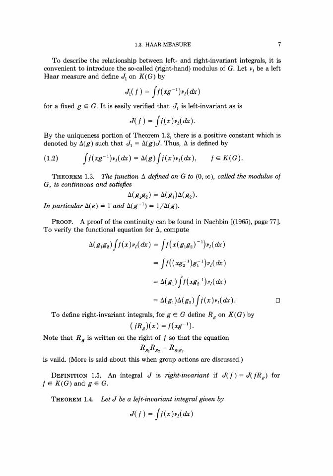
To describe the relationship between left- and right-invariant integrals, it is convenient to introduce the so-called (right-hand) modulus of G. Let v1 be a left Haar measure and define J 1 on K (G) by

for a fixed g E G. It is easily verified that J1 is left-invariant as is

J(f) = jf(x)v1(dx).

By the uniqueness portion of Theorem 1.2, there is a positive constant which is denoted by b.(g) such that J 1 = b.(g)J. Thus, b. is defined by

(1.2) feK(G).

THEOREM 1.3. The function b. defined on G to (0, oo ), called the modulus of G, is continuous and satisfies

b.(glg2) = b.(gl )b.(g2).

In particular b.( e)= 1 and b.(g- 1) = 1/b.(g).

PROOF. A proof of the continuity can be found in Nachbin [(1965), page 77]. To verify the functional equation for b., compute

b.(glg2) jf(x)vz(dx) = jf(x(g1g 2 )- 1)v1(dx)

= jf((xg2 1 )g~ 1 )v1 (dx)

= b.(g1) jf(xg2 1 )vz(dx)

= b.(gi)b.(g2) jf(x)vz(dx).

To define right-invariant integrals, forgE G define Rg on K(G) by

(fRg)(x) = f(xg- 1 ).

Note that R g is written on the right of f so that the equation

Rg,Rg2 = Rg,g2

is valid. (More is said about this when group actions are discussed.)

0

DEFINITION 1.5. An integral J is right-invariant if J( f) = J( fRg) for f E K (G) and g E G.

THEOREM 1.4. Let J be a left-invariant integral given by

J(f) = jf(x)v1(dx)

8 INTEGRALS AND THE HAAR MEASURE

and let ~ be the modulus of G. Then the integral J 1 defined by

is right-invariant and satisfies

(1.3)

for f E K(G).

PROOF. That J 1 is right-invariant follows from the definition of ~ and the calculation

J1( fRg) = jf(xg- 1 )~(x- 1 )v1 (dx)

1 = jf(xg·- 1) ~(xg-Ig) v1(dx)

1 f(xg· 1)

= ~(g) j ~(xg-1) Pz(dx)

~(g)Jf(x) = ~(g) ~(x) v1(dx) = J1(f ).

A proof of the second equation can be found in Nachbin [(1965), page 78]. D

Equation (1.3) establishes a relationship between left and right Haar measure. Namely, if v 1 is a left Haar measure, then

(1.4)

is a right Haar measure. Further if vr is a right Haar measure, a similar construction shows that

(1.5)

is a left Haar measure. Before turning to a few examples, we discuss the important special case of

compact groups. Here is a characterization of compact groups in terms of Haar measure.

THEOREM 1.5. In order that G be compact, it is necessary and sufficient that there exist a finite Haar measure [that is, p,(G) < + oo].

PROOF. See Nachbin [(1965), page 75]. D

Let ~ be the modulus of a compact group G. We claim that ~ = 1. To see this, recall that ~ is a continuous function from G into (0, oo) which satisfies

~(g1g2) = ~(g1)~(g2),

1.3. HAAR MEASURE 9

that is, Ll is a group homomorphism. Thus H = {Ll(g)jg E G} is a subgroup of the multiplicative group (0, oo ). However, Il is compact as it is the continuous image of the compact set G. If H =f=. {1 }, then there exists a E H such that a > 1. Hence an E H for n = 1, 2, .... But { an!n = 1, 2, ... } does not contain a convergent subsequence which contradicts the compactness of H. Thus L1 = 1 for any compact group G. Therefore all right Haar measures are left Haar measures and conversely. In these notes, the Haar measure on a compact group G is always normalized so that J.L( G) = 1, that is, the Haar measure is taken to be a probability measure.

Here are some examples of left and right Haar measures.

EXAMPLE 1.7. Take G to be the vector space Rn with addition as the group operation. Then ordinary Lebesgue measure on Rn is both left- and rightinvariant (the group here is commutative) and so the modulus is L1 = 1. 0

EXAMPLE 1.8. If G is any finite or denumerable discrete group, then counting measure is both left- and right-invariant and so the modulus is 1. 0

EXAMPLE 1.9. For this example, take G = Gln as in Example 1.3. Let dx denote Lebesgue measure restricted to Gln with Gln regarded as a subset of .Pn n· Since G is open in .Pn, n• Gln has positive Lebesgue measure. Define an inte~al J by

dx J(f) = jf(x)jdet(x)ln·

The claim is that J is both left- and right-invariant. To see this, first consider

dx J(Lgf) = jf(g-lx) jdet(x)jn

and make the change of variables y = g 1x so x = gy. To calculate the Jacobian of this transformation (defined by g), write x as a column vector

where xi is the ith column of x and do the same with y. In this notation, the equation x = gy becomes

g

g

where the elements not indicated in the n2 X n2 matrix are 0. Obviously this


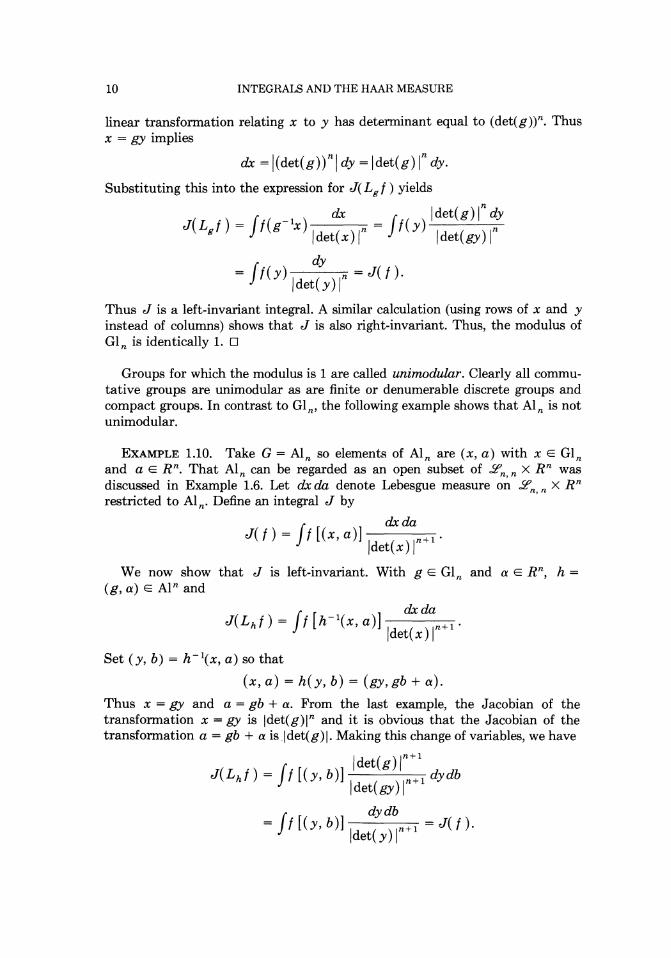
linear transformation relating x to y has determinant equal to (det(g)t. Thus x = gy implies

dx =j(det(g)tjdy =ldet(g)ln dy.

Substituting this into the expression for J(Lgf) yields

dx ldet(g) Indy J(Lgt) = jf(g-lx) ldet(x)ln = jf(y) ldet(gy)ln

dy = j f ( Y) I det( y) ( = .J(f ) ·

Thus J is a left-invariant integral. A similar calculation (using rows of x and y instead of columns) shows that J is also right-invariant. Thus, the modulus of Gln is identically 1. 0

Groups for which the modulus is 1 are called unirrwdular. Clearly all commutative groups are unimodular as are finite or denumerable discrete groups and compact groups. In contrast to Gl n' the following example shows that Al n is not unimodular.

EXAMPLE 1.10. Take G = Aln so elements of Aln are (x, a) with x E Gln and a E Rn. That Aln can be regarded as an open subset of .Pn, n X Rn was discussed in Example 1.6. Let dx da denote Lebesgue measure on .Pn n X Rn restricted to Aln. Define an integral J by '

dxda

J(f) = jt[(x,a)] ldet(x)ln+I"

We now show that J is left-invariant. With g E Gln and a ERn, h =

(g, a) E Aln and

f dxda J(Lhf)= f[h- 1(x,a)] n+l"

ldet(x) I Set (y, b)= h- 1(x, a) so that

(x, a)= h(y, b)= (gy, gb +a).

Thus x = gy and a= gb +a. From the last example, the Jacobian of the transformation x = gy is ldet(gW and it is obvious that the Jacobian of the transformation a= gb + a is ldet(g)l. Making this change of variables, we have

/det(g) /n+l J( L h f) = J f[ ( Y, b)] n + 1 dy db

/det(gy) /

f dydb = t[(y, b)] /det(y)/n+l = J(f).

1.4. MULTIPLIERS AND RELATIVELY INVARIANT INTEGRALS 11

A similar (but slightly different) calculation shows that

dxda J 1(f) = jt[(x,a)] !det(x)ln

is a right-invariant integral. From Equation (1.4), it follows that the modulus of Aln is

1 A(x, a)= !det(x)l" D

Other examples of invariant integrals are given in the next section after the discussion of multipliers and relatively invariant integrals.

1.4. Multipliers and relatively invariant integrals. The modulus A of a topological group G provides an example of a multiplier, namely a continuous homomorphism of G into the multiplicative group of (0, oo ). Multipliers play the role of Jacobians for some integrals on K(G).

DEFINITION 1.6. A function x defined on G to (0, oo) is a multiplier if x is continuous and x(g1g2 ) = x(g1)x(g2 ) for g1, g2 E G.

It is clear that x( e) = 1 and x(g1g 2 ) = x(g2g1) for any multiplier x, so that x(g 1) = 1/x(g). Further, x(G) = {x(g)jg E G} is a subgroup of (0, oo). Thus, if G is compact, x( G) must be a compact subgroup of (0, oo) and thus x( G) = { 1}. Hence the trivial multiplier, x = 1, is the only multiplier defined on a compact group.

DEFINITION 1.7. An integral Jon K(G) is relatively (left) invariant with multiplier x if for each g E G1,

J(Lgf) = jt(g- 1x)m(dx) = x(g) jt(x)m(dx) = x(g).J(f ).

The relationship between invariant and relatively invariant integrals is given in the following result.

THEOREM 1.6. Let X be a multiplier on G.

(i) If Ji I)= ff(x)m(dx) is relatively invariant with multiplier x, then

J(f) = j f(x )x(x- 1 )m( dx)

is left-invariant. (ii) If J( f)= ff(x)v1(dx) is left-invariant, then

Jl(f) = jt(x)x(x)v1(dx)

is relatively invariant with multiplier x.

12 INTEGRALS AND THE HAAH MEASURE

PROOF. Only the proof of (i) is given, as the proof of (ii) is similar. For gE G,

J(Lgt) = jf(g ___ 1x)x(x- 1 )m(d.x) = jf(g- 1x)x((g- 1x)- 1g- 1 )m(d.x)

= X ( g- 1 ) X (g) f f (X ) X (X- 1 ) m ( d.x ) = J( f ) ·

Thus, J is left invariant. D

Theorem 1.6 shows how to construct a relatively invariant integral with a given multiplier from a left-invariant measure, and conversely. In practice, it is the converse which is somewhat more useful since it provides a very useful method of constructing a left-invariant integral in some cases. Here is a rather informal description of the method which is used below to construct a leftinvariant measure on the group a; of Example 1.4. Suppose the topological group G is subset of a Euclidean space Rm such that G has positive Lebesgue measure. Define a integral on K(G) by

where d.x denotes Lebesgue measure restricted to G. If we can show that

(1.6) 1 f(g- 1x) d.x = x(g) 1 f(x) d.x forgE G, G G

then

is left-invariant. The verification of (1.6) is ordinarily carried out by changing variables and computing a Jacobian.

One can also define relatively right-invariant integrals, but their relationship to relatively left integrals follows from (1.5) and the equation

(1.7) m(d.x) = x(x)v1(d.x),

which relates the left Haar measure v1 and the measure m which defines a relatively invariant integral with multiplier X· For this reason, relatively rightinvariant integrals are not mentioned explicitly.

It follows from Theorem 1.6 that the problem of describing all the relatively invariant integrals on K(G) can be solved by first exhibiting one relatively invariant integral and then describing all the multipliers on G. This program is carried out in some examples that follow. Before turning to these examples, it is useful to describe a few general facts concerning multipliers.

THEOREM 1.7. Suppose the topological group G is the direct product G1 X G2

of two topological groups [that is, each g E G has the form g = (gp g 2) with gi E G; and the group operation is go h = (g1h1, g 2 h2 ) where g = (g1, g 2 ) and


h = (h1, h 2)]. The topology on G is assumed to be the product topology. Then x is a multiplier on G iff (1.8) X [ (gp g2)] = Xl(gl)xig2),

where Xi is a multiplier on G;, i = 1, 2.

PROOF. If x has the form (1.8), it is clear that x is a multiplier. Conversely, suppose that x is a multiplier. For g = (g1, g 2 ) E G, write

(gl, g2) = (gP ez)( el, g2),

where ei is the identity in Gi, i = 1, 2. Then consider

X1(g1) = x[(gv e2)], gl E Gv

X2(g2)=x[(ePg2)], g2EGz.

The continuity of Xi on Gi follows since xis continuous and Xi is x restricted to a closed subset of G. That (1.8) holds follows since x is a homomorphism. D

Also observe that if x is a multiplier on G and H is a closed subgroup of G, then the restriction of x to H is a multiplier on H. In particular, if H is a compact subgroup of G, then x( h) = 1 for all h E H since compact groups have only trivial multipliers.

EXAMPLE 1.11. In this example, all the relatively invariant integrals on Rn are computed. Because Rn is an n-fold product group, Theorem 1.7 shows that it is sufficient to treat the case n = 1. Thus, suppose that x 1 is a continuous function from R1 to (0, oo) which satisfies the equation

x~(x + y) = x~(x)x~(y). Taking logs of both sides of this leads to

logx 1(x + y) = f(x + y) = f(x) + f(y) for x, y E R1. This is the well known Cauchy functional eqllation which has the solution (because f is continuous)

f(x) =ex, where c is some real number. Thus,

x 1(x) = exp[cx], X E R\ where c is a fixed real number. Applying Theorem 1.7 shows that x is a multiplier on Rn iff x has the form

x(u) = exp[ ~ciul where u E Rn has coordinates u1, ... , un and c1, ... , en are fixed real numbers. Thus, a Radon measure m is relatively invariant with multiplier x given above iff

m(du) = c0x(u) du,

where c0 is a fixed constant and du is Lebesgue measure on Rn.


When G is the product multiplicative group (0, oo t, the continuous isomorphism cp: G ~ Rn given by

cp(x) =

logxn

can be used to show that the measure

X E (0, oot,

is right- and left-invariant on G. Further, x is a multiplier on G iff x has the form

n

x(x) = f1 (x;)\ i~l

where c1, ••• , en are fixed real numbers. Thus, all the relatively invariant integrals on K (G) are known. D

EXAMPLE 1.12. Consider G = Gl n as in Example 1.3 so

dx p (dx) -

1 - I det( X ) In

is left- and right-invariant. To describe all the multipliers on Gln, the functional equation

( 1.9) X ( xy) = X (X )x ( y), X, y E G l n,

must be solved. To this end, recall the singular value decomposition of an n X n matrix x E Gln; it is

x = aD/3,

where a, f3 E On and D is an n X n diagonal matrix with positive diagonal elements [for example, see Eaton (1983), page 58]. Thus if x is continuous and satisfies (1.9), then

X ( x) = X ( aD/3) = X (a )x (D) X ( /3) = X (D)

since a and /3 are both elements of the compact group on so x(a) = x(/3) = 1. Now, write D as

n

D = fiDi(dJ, i=l

where di is the ith diagonal of D and Di( di) has ith diagonal equal to di and all other diagonal elements equal to 1. Then, because Di(dJ E Gln,

x(D) = x(}]ni(dJ) = Qx(DJd;)).


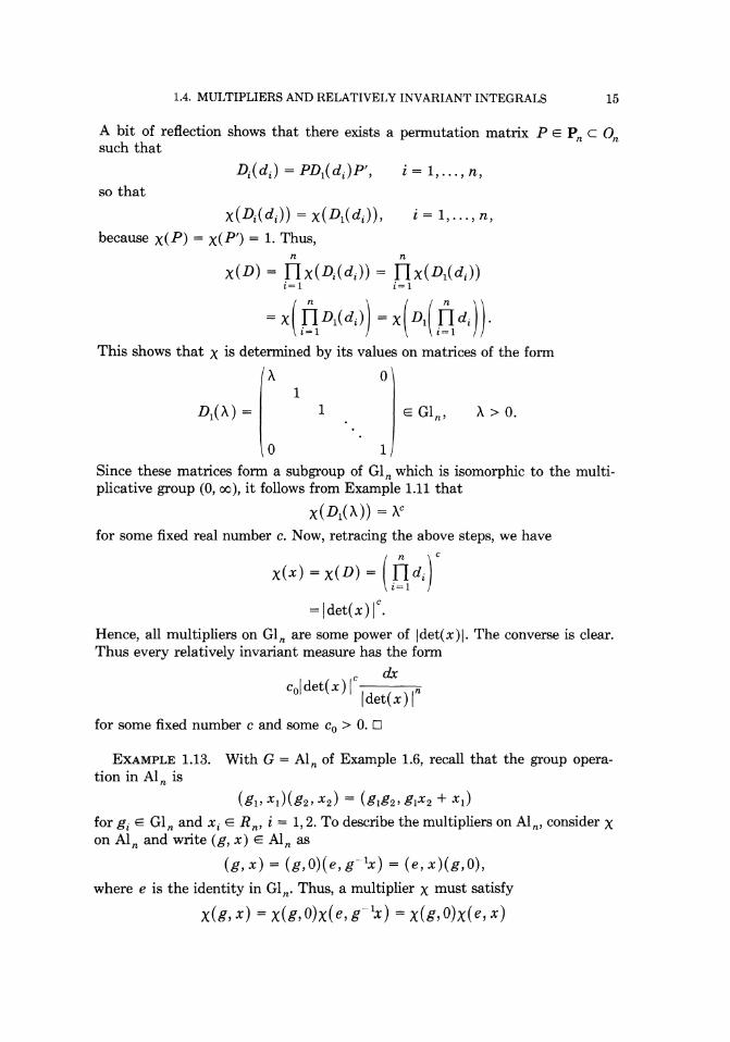
A bit of reflection shows that there exists a permutation matrix P E P c 0 n n such that

i = 1, ... , n, so that

x(Di(dJ) = x(D1(dJ), because x(P) = x(P') = 1. Thus,

i = 1, ... , n,

n n

x(D) = flx(Di(dJ) = Tix(Dl(dJ) i= 1 i= 1

This shows that x is determined by its values on matrices of the form

i\ 0 1

1 i\ > 0.

0 1

Since these matrices form a subgroup of Gln which is isomorphic to the multiplicative group (0, oo ), it follows from Example 1.11 that

x(Dl(i\)) = i\c

for some fixed real number c. Now, retracing the above steps, we have

x(x) = x(D) = (l]dir

= I det( x) I c.

Hence, all multipliers on Gln are some power of !det(x)l. The converse is clear. Thus every relatively invariant measure has the form

c dx c0 1 det( X) I n

ldet(x) I for some fixed number c and some c0 > 0. D

EXAMPLE 1.13. With G = Aln of Example 1.6, recall that the group operation in Al n is

(gu X1)(g2, x2) = (glg2, g1X2 + xl)

for gi E Gln and xi ERn, i = 1, 2. To describe the multipliers on Aln, consider X on Aln and write (g, x) E Aln as

( g, x ) = ( g, 0) ( e, g- 1x ) = ( e , x) ( g, 0) ,

where e is the identity in Gln. Thus, a multiplier x must satisfy

x(g,x) =x(g,o)x(e,g- 1x) =x(g,O)x(e,x)


so

x ( e, g 1x) = x ( e, x)

for all g E Gl,. Letting g- 1 converge to 0, the continuity of x implies that

1 = x(e,O) = x(e, x), X E R".

Hence

x(g,x) = x(g,O), g E Gl,.

But g ~ x(g, 0) defines a multiplier on Gl, so by the previous example,

x(g,x) =ldet(g)lc

for some fixed real number c. Conversely, it is clear that such a function on Al, is a multiplier. Thus, all the multipliers on Al, have been ·given. D

ExAMPLE 1.14. The final example of this chapter concerns a; c Gl,. The left and right Haar measures, the modular function and all the multipliers for a; are derived here. We are going to use the method described after the proof of Theorem 1.6. For x E a;j., x has the form

Xu D 0

X21 X22 0 x=

x,l x,2 x,,

with X;;> 0 and x;1 E R", i > j. Let dx denote Lebesgue measure restricted to the set of such x's in n(n + 1)/2 dimensional space. Define an integral Jon K(a;j.) by

J(f ) = f f (X) dx

and forgE a;, consider

With y = g-·lx sox= gy, the Jacobian of this transformation on n(n + 1)/2 coordinate space is

n

Xo(g) = TI gt;, i~l

where gw ... , g,, are the diagonal elements of g E a; [see Eaton (1983), page 171]. Hence dx = x 0(g) dy so that

J(I_,gf) = Xo(g)J( f).

From Theorem 1.6, we have that

(1.10)


is a left Haar measure on G;j. c Gln. The modulus of G~ is computed using the definition (1.2). Thus, consider

dx jf(xg- 1)v1(dx) = jf(xg- 1)-(-)

Xo x

and let y = xg ·· 1 so x = yg. The Jacobian of this transform is n

xl(g) = ngg-i+l, i= 1

where gw ... , gnn are the diagonal elements of g. Making this change of variables in the above integral yields

jf(xg- 1)vz(dx) = jf(y)x1(g) t ) Xo yg

= X1(g) jf(y)~ Xo(g) Xo(Y)

X1(g) f = -( -) f(x)v1(dx).

Xo g

Thus, by definition, the modulus of G;j. is

(l.ll) b.(g) = X1(g) = Ilgg-2i+l xo(g) i= 1

so a right Haar measure is

(1.12) 0

Here is a characterization of the multipliers on G;j. c Gln.

THEOREM 1.8. All multipliers on G;j.c Gln have the form n

x(g) = n (gi;)\ i=l

where c1, ••• , en are fixed real numbers. Conversely, any such function is a multiplier.

PROOF. That such a function is a multiplier is easily checked. To show that all multipliers have the claimed form, we argue by induction. For n = 1, G;j. = (0, oo) and the assertion follows from Example 1.11. Assume the result is true for G;j.c Gln and consider G;j.c Gln+J· ForgE G;j.c Gln+l> partition gas

g = ( ~~~ X~2)' where x11 is n X n, x21 is 1 X n and x22 is in (0, oo ). With e denoting the n x n


identity matrix, observe that

( ::: x~J = ( x~1 ~ )( x:1 x~J 0 ) (Xu 0). x 22 0 1

Thus, if x is a multiplier,

(Xu X 0

0 )x(xu x12 0 ~) so that

x( e o ) = x( e 1 X21 X22 X21Xu

Letting x111 converge to 0, the continuity of x implies that

X ( x:1 x~2 ) = X ( ~ x~2 ) • But, the function

x22~x(~ x~J defines a multiplier on (0, oo ), so

( e 0 ) = (x22rn+I X 0 x22

for some real c n + 1. Also, the function

x11 ~ X ( x~ 1 ~) defines a multiplier on a; c Gln. Since the diagonal elements of Xu are gw ... , gn, n and x22 = gn+ 1, n+ 1, using the induction hypothesis, we have

x(g)=x(;~~ x~z)=x(xo1 nx(~ x~2) (

n ) n+ 1 = f1g~· g~Yi = n g{i·

!=1 i=l

This completes the proof. 0

That the compact group On has a unique left- and right-invariant probability measure follows from the general theory of Haar measure. However, the explicit construction of this probability, in terms of a "coordinate system" for on is a bit technical and requires some familiarity with differential forms. This topic is not discussed here, but in subsequent material, it is shown how to construct a random orthogonal matrix in On whose distribution is exactly the Haar measure on On. This construction involves the multivariate normal distribution.

Documents

Integrals and the Haar Measure - Project Euclid