Integrability in QFT and AdS/CFT

Lecture Notes

ABGP Doctoral School, 2014

Niklas Beisert

c© 2014 Niklas Beisert, ETH Zurich

This document as well as its parts is protected by copyright.Reproduction of any part in any form without prior writtenconsent of the author is permissible only for private,scientific and non-commercial use.

Contents

0 Overview 40.1 Introduction . . . . . . . . . . . . . . . . . . . . . . . . . . . . . . . 40.2 Contents . . . . . . . . . . . . . . . . . . . . . . . . . . . . . . . . . 50.3 Literature . . . . . . . . . . . . . . . . . . . . . . . . . . . . . . . . 5

1 Classical Integrability 1.11.1 Hamiltonian Mechanics . . . . . . . . . . . . . . . . . . . . . . . . . 1.11.2 Integrals of Motion . . . . . . . . . . . . . . . . . . . . . . . . . . . 1.21.3 Liouville Integrability . . . . . . . . . . . . . . . . . . . . . . . . . . 1.21.4 Comparison of Classes . . . . . . . . . . . . . . . . . . . . . . . . . 1.41.5 Structures of Integrability . . . . . . . . . . . . . . . . . . . . . . . 1.5

2 Integrable Field Theory 2.12.1 Classical Field Theory . . . . . . . . . . . . . . . . . . . . . . . . . 2.12.2 Spectral Curves . . . . . . . . . . . . . . . . . . . . . . . . . . . . . 2.5

3 Integrable Spin Chains 3.13.1 Heisenberg Spin Chain . . . . . . . . . . . . . . . . . . . . . . . . . 3.13.2 Coordinate Bethe Ansatz . . . . . . . . . . . . . . . . . . . . . . . . 3.63.3 Generalisation . . . . . . . . . . . . . . . . . . . . . . . . . . . . . . 3.14

4 Quantum Integrability 4.14.1 R-Matrix Formalism . . . . . . . . . . . . . . . . . . . . . . . . . . 4.14.2 Other Types of Bethe Ansatze . . . . . . . . . . . . . . . . . . . . . 4.12

5 AdS/CFT Integrability 5.1

3

Integrability in QFT and AdS/CFT Chapter 0ABGP Doctoral School, 2014 Niklas Beisert

17. 12. 2014

0 Overview

0.1 Introduction

What is integrability?

• . . . a peculiar feature of some theoretical physics models.• . . . makes calculations in these models much more feasible in principle and in

practice; it is also known as solvability.• . . . allows to compute some quantities exactly and analytically rather than

approximately and numerically.• . . . is a hidden enhancement of symmetries which constrain the motion

substantially or completely.• . . . is the absence of chaotic motion.• . . . is a colourful mixture of many subjects and techniques from mathematics to

physical phenomena.• . . . a lot of fun.

Which classes of models are integrable?

• some classical mechanics models, e.g.: free particle, harmonic oscillator, spinningtop, planetary motion, . . . .1

• some (1 + 1)-dimensional classical field theories, e.g.: KdV, sine-Gordon,Einstein gravity, sigma models on coset spaces, classical magnets, string theory.• some quantum mechanical models, e.g. the quantum versions of the above

classical mechanics models.• some (1 + 1)-dimensional quantum field theories, e.g. most of the quantum

counterparts of the above classical field theories, except cases where integrabilityis spoiled by quantum effects.• some 2-dimensional models of statistical mechanics, e.g. 6-vertex model, 8-vertex

model, alternating sign matrices, loop models, Ising model, . . . .• D = 4 self-dual Yang–Mills theory.• D = 4, N = 4 maximally supersymmetric Yang–Mills theory in the planar limit

and the AdS/CFT dual string theory on AdS5 × S5.

One observes that integrability is a phenomenon largely restricted totwo-dimensional systems. There are some higher-dimensional exceptions, but mostof them have some implicit two-dimensionality (self-duality, planar limit).

1Most models discussed in lectures and textbooks are in fact integrable, most likely becausethey can be solved easily and exactly.

4

0.2 Contents

1. Classical Integrability (1.5h)2. Integrable Field Theory (2.5h)3. Integrable Spin Chains (4.5h)4. Quantum Integrability (3.0h)5. AdS/CFT Integrability (2.5h)

0.3 Literature

• G. Arutyunov, “Students Seminar: Classical and Quantum Integrable Systems”• O. Babelon, D. Bernard, M. Talon, “Introduction to Classical Integrable

Systems”, Cambridge University Press (2003)• N. Beisert, “The Dilatation Operator of N = 4 super Yang-Mills Theory and

Integrability”, Phys. Rept. 405, 1–202 (2004),http://arxiv.org/abs/hep-th/0407277.• N. Reshetikhin, “Lectures on the integrability of the 6-vertex model”,http://arxiv.org/abs/1010.5031.• L.D. Faddeev, “How Algebraic Bethe Ansatz Works for Integrable Model”,http://arxiv.org/abs/hep-th/9605187.• N. Beisert et al., “Review of AdS/CFT Integrability: An Overview”,http://arxiv.org/abs/1012.3982.• . . .

5

Integrability in QFT and AdS/CFT Chapter 1ABGP Doctoral School, 2014 Niklas Beisert

03. 12. 2014

1 Classical Integrability

Here we discuss integrability for a system of classical mechanics with finitely manydegrees of freedom. Although this will not be the main subject of this course, it isvery instructive because there is a clear notion of integrability in this case whichlays the foundation for the more elaborate cases of field theory and quantummechanics discussed later.

1.1 Hamiltonian Mechanics

We start by defining a classical mechanics system in Hamiltonian formulation. Itconsists of a phase space M of dimension 2n and a Hamiltonian functionH :M→ R. Phase space is defined by a set of coordinates qk and momenta pkwith k = 1, . . . , n.

A solution of the system is a curve (qk(t), pk(t)) in phase space which obeys theHamiltonian equations of motion

qk =∂H

∂pk, pk = −∂H

∂qk. (1.1)

It is convenient to introduce Poisson brackets which map a pair of functions F , Gon phase space to another function on phase space1

{F,G} :=∂F

∂pk

∂G

∂qk− ∂F

∂qk∂G

∂pk. (1.2)

The Poisson brackets are anti-symmetric and they obey the Jacobi identity{{F,G}, H

}+{{G,H}, F

}+{{H,F}, G

}= 0. (1.3)

The Poisson brackets allows to write the equations of motion in a compact anduniform fashion as

d

dtqk = {H, qk}, d

dtpk = {H, pk}. (1.4)

More generally, the time-dependence of a function F (q, p, t) evaluated on asolution (qk(t), pk(t)) reads2

d

dtF =

∂F

∂t+ {H,F}. (1.5)

1The Poisson brackets are often defined by specifying the canonical relations {pk, ql} = δklalong with the trivial ones {pk, pl} = {qk, ql} = 0.

2To make proper sense of the above equations of motion one should introduce the coordinatefunctions qk(q, p, t) := qk, pk(q, p, t) := pk whose partial derivatives w.r.t. time vanish,∂qk/∂t = ∂pk/∂t = 0.

1.1

1.2 Integrals of Motion

For a time-independent Hamiltonian, H = 0, the function H is an integral ofmotion or conserved quantity

d

dtH =

∂H

∂t+ {H,H} = 0. (1.6)

The immediate benefit is that solutions are constrained to a hypersurface of Mdefined by H = E = const. (constant energy). It is therefore easier to findsolutions.

Depending on the model, further (time-independent)3 integrals of motion Fk canexist

d

dtFk = {H,Fk}

!= 0. (1.7)

This gives additional constraints Fk = fk = const. and motion takes place on aneven lower-dimensional hypersurface which is called a level set

Mf := {x ∈M;Fk(x) = fk}. (1.8)

By construction, the Hamiltonian H is among them and one may identify F1 = H.

Additional simplifications come about when the integrals are in involution or(Poisson) commute

{Fk, Fl} = 0. (1.9)

This allows to consistently define solutions (q, p) depending on several timevariables tk such that time-dependence for any function G is determined by4

d

dtkG =

∂G

∂tk+ {Fk, G}. (1.10)

Finding integrals of motion is all but straight-forward:

• They are often found by trial and error based on a suitable ansatz.• Noether’s theorem implies the existence of a conserved quantity for each global

symmetry of the system.5

1.3 Liouville Integrability

A system with 2n-dimensional phase space M is called (Liouville) integrable if ithas

3Throughout this course we will implicitly assume that functions of phase space have noexplicit time dependence.

4 Consistency requires that d/dtk commutes with d/dtl which is guaranteed by {Fk, Fl} = 0by means of the Jacobi identity.

5Additional conserved quantities can often be regarded as a consequence of additional hiddensymmetries of the system.

1.2

• n independent6

• everywhere differentiable• integrals of motion Fk• in involution, {Fk, Fl} = 0.

Such a system is solvable by quadratures, i.e. it suffices to solve a finite number ofalgebraic equations and integrals.

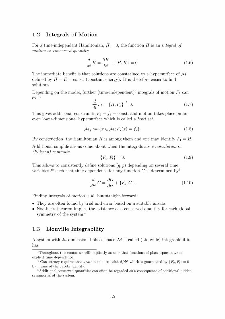
For integrable systems the following theorem holds: If the level setMf is compact,it is diffeomorphic to the n-dimensional torus T n, the so-called Liouville torus.7

MMf

(1.11)

For an integrable system, we can define a set of n time functions T k on phasespace such that {Fk, T l} = δlk. These differential equations define the T k on eachlevel set. Furthermore, the time functions can be defined across the level sets byimposing the differential equations {T k, T l} = 0. Suitable functions can beconstructed thanks to the Jacobi identities. Altogether we have

{Fk, T l} = δlk, {Fk, Fl} = {T k, T l} = 0, (1.12)

which tells us that the map (qk, pk)→ (T k, Fk) is a canonical transformation.

Note that the time functions are in general multiple-valued on phase space. Goingaround a non-trivial cycle of a level set, the times jump by a definite amount,8

given by the period matrix. In that sense, the time functions T k are uniquelydefined on the universal cover Rn of the level sets. Conversely, the level set is thequotient of Rn by the lattice defined by the periods.

T 1T 2

ω1

ω2

T 1

T 2

(1.13)

A useful corollary of integrability is that motion on the level set torus is linear since

{H,T k} = {F1, Tk} = δk1 , (1.14)

6A function of phase space is called independent of a set of functions if it cannot be written asa function of the values of the other functions. For instance, the total angular momentumJ2 = J2

x + J2y + J2

z is dependent on the components {Jx, Jy, Jz} of the angular momentum.Moreover, a constant function is always dependent, even on the empty set of functions.

7This theorem follows by considering the vector fields associated to the integral of motions Fk

defined by the operation {Fk, ·}. By construction, the vector fields act within the level set andcommute with each other. It is well-known that a compact manifold of dimension n which admitsn commuting vector fields is diffeomorphic to the torus Tn.

8The differential equations determine the time functions locally up to a constant shift.

1.3

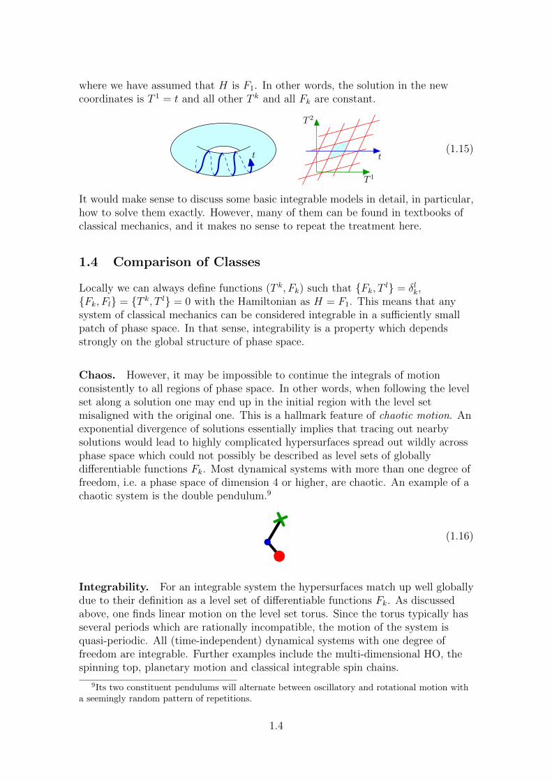
where we have assumed that H is F1. In other words, the solution in the newcoordinates is T 1 = t and all other T k and all Fk are constant.

t

T 1

t

T 2

(1.15)

It would make sense to discuss some basic integrable models in detail, in particular,how to solve them exactly. However, many of them can be found in textbooks ofclassical mechanics, and it makes no sense to repeat the treatment here.

1.4 Comparison of Classes

Locally we can always define functions (T k, Fk) such that {Fk, T l} = δlk,{Fk, Fl} = {T k, T l} = 0 with the Hamiltonian as H = F1. This means that anysystem of classical mechanics can be considered integrable in a sufficiently smallpatch of phase space. In that sense, integrability is a property which dependsstrongly on the global structure of phase space.

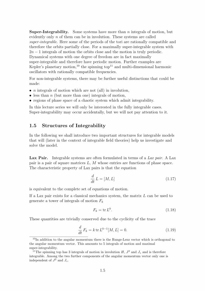
Chaos. However, it may be impossible to continue the integrals of motionconsistently to all regions of phase space. In other words, when following the levelset along a solution one may end up in the initial region with the level setmisaligned with the original one. This is a hallmark feature of chaotic motion. Anexponential divergence of solutions essentially implies that tracing out nearbysolutions would lead to highly complicated hypersurfaces spread out wildly acrossphase space which could not possibly be described as level sets of globallydifferentiable functions Fk. Most dynamical systems with more than one degree offreedom, i.e. a phase space of dimension 4 or higher, are chaotic. An example of achaotic system is the double pendulum.9

(1.16)

Integrability. For an integrable system the hypersurfaces match up well globallydue to their definition as a level set of differentiable functions Fk. As discussedabove, one finds linear motion on the level set torus. Since the torus typically hasseveral periods which are rationally incompatible, the motion of the system isquasi-periodic. All (time-independent) dynamical systems with one degree offreedom are integrable. Further examples include the multi-dimensional HO, thespinning top, planetary motion and classical integrable spin chains.

9Its two constituent pendulums will alternate between oscillatory and rotational motion witha seemingly random pattern of repetitions.

1.4

Super-Integrability. Some systems have more than n integrals of motion, butevidently only n of them can be in involution. These systems are calledsuper-integrable. Here some of the periods of the tori are rationally compatible andtherefore the orbits partially close. For a maximally super-integrable system with2n− 1 integrals of motion the orbits close and the motion is truly periodic.Dynamical systems with one degree of freedom are in fact maximallysuper-integrable and therefore have periodic motion. Further examples areKepler’s planetary motion,10 the spinning top11 and multi-dimensional harmonicoscillators with rationally compatible frequencies.

For non-integrable systems, there may be further useful distinctions that could bemade:

• n integrals of motion which are not (all) in involution,• less than n (but more than one) integrals of motion,• regions of phase space of a chaotic system which admit integrability.

In this lecture series we will only be interested in the fully integrable cases.Super-integrability may occur accidentally, but we will not pay attention to it.

1.5 Structures of Integrability

In the following we shall introduce two important structures for integrable modelsthat will (later in the context of integrable field theories) help us investigate andsolve the model.

Lax Pair. Integrable systems are often formulated in terms of a Lax pair. A Laxpair is a pair of square matrices L, M whose entries are functions of phase space.The characteristic property of Lax pairs is that the equation

d

dtL = [M,L] (1.17)

is equivalent to the complete set of equations of motion.

If a Lax pair exists for a classical mechanics system, the matrix L can be used togenerate a tower of integrals of motion Fk

Fk = trLk. (1.18)

These quantities are trivially conserved due to the cyclicity of the trace

d

dtFk = k trLk−1[M,L] = 0. (1.19)

10In addition to the angular momentum there is the Runge-Lenz vector which is orthogonal tothe angular momentum vector. This amounts to 5 integrals of motion and maximalsuper-integrability.

11The spinning top has 3 integrals of motion in involution H, J2 and Jz and is thereforeintegrable. Among the two further components of the angular momentum vector only one isindependent of J2 and Jz.

1.5

For systems with finitely many degrees of freedom, only finitely many of thegenerated charges can be independent.

Alternatively, the Lax equation is equivalent to the statement that time evolutionof L is generated by a similarity transformation. Therefore the eigenvaluespectrum and the characteristic polynomial of L are conserved. Note that thelatter is a function of the Fk.

Having a Lax pair formulation of integrability is very convenient, but

• inspiration is needed to find it,• its structure is hardly transparent,• it is not at all unique,• the size of the matrices is not immediately related to the dimensionality of the

system.

Therefore, the concept of Lax pairs does not provide a means to decide whetherany given system is integrable (unless one is lucky to find a sufficiently large Laxpair).

Classical r-matrix. For integrability we not only need sufficiently many globalintegrals of motion Fk, but they must also be in involution, {Fk, Fl} = 0. In theformulation of integrability in terms of a Lax pair L,M ∈ End(V ), this isequivalent to the statement

{L1, L2} = [r12, L1]− [r21, L2]. (1.20)

The statement is defined on the tensor product space End(V ⊗ V ) of two matrices,and the classical r-matrix r12 is a particular element of this space whose entries arefunctions on phase space.12 Furthermore, L1 := L⊗ 1, L2 := 1⊗ L, andr21 := P (r12) denotes the permutation of the two spaces for the r-matrix. Notethat the r-matrix is by no means uniquely defined by the equation.13 Much like forthe Lax pair, there is no universal method to obtain the r-matrix.

From the above equation it follows straight-forwardly that

{trLk, trLl} = 0. (1.21)

There is a useful graphical representation of the equation where matrices areobjects with one ingoing and one outgoing leg. Connecting two legs corresponds toa product of matrices, whereas two matrices side by side correspond to a tensorproduct. Consequently, the classical r-matrix will be an object with two ingoing

12The tensor product A⊗B of two matrices with elements Aac, B

bd has the elements

(A⊗B)abcd = AacB

bd, where ab and cd are combined indices enumerating a basis for the tensor

product space.13For example, one can add an operator of the form 1⊗X + L⊗ Y where X and Y are

arbitrary matrices.

1.6

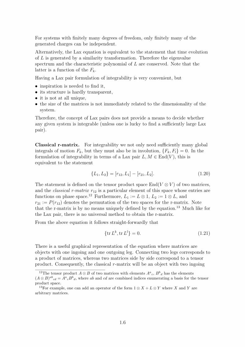
and outgoing legs, and the above equation reads

{L1 1, L2 2

}= r

L1

22

1− r

L1

22

1

− rL2

11

2+ r

L2

11

2. (1.22)

Many relationship can be conveniently expressed and proved using this graphicalnotation. We shall make extensive use of it in the context of integrable spin chains.

Example. Consider a harmonic oscillator with frequency ω. A Lax pair is givenby

L =

(+p ωqωq −p

), M =

(0 −1

2ω

+12ω 0

). (1.23)

The Lax equation is equivalent to the equation of motion of the harmonic oscillator

p = −ω2q, ωq = ωp. (1.24)

The resulting integrals of motion read

F1 = 0,

F2 = 2p2 + 2ω2q2 = 4H,

F3 = 0,

F4 = 2(p2 + ω2q2)2 = 8H2,

. . . . (1.25)

Here F1 and F3 are trivial and can be ignored. The first and only non-trivialintegral of motion F2 is the Hamiltonian. The higher even powers are merelypowers of the Hamiltonian which are not independent integrals of motion.

For this system, a classical r-matrix is given by

r12 =1

q

(0 10 0

)⊗(

0 01 0

)− 1

q

(0 01 0

)⊗(

0 10 0

). (1.26)

The above commutators with the Lax matrix L then agrees precisely with thePoisson brackets

{L1, L2} = ω

(1 00 −1

)⊗(

0 11 0

)− ω

(0 11 0

)⊗(

1 00 −1

). (1.27)

1.7

Integrability in QFT and AdS/CFT Chapter 2ABGP Doctoral School, 2014 Niklas Beisert

03. 12. 2014

2 Integrable Field Theory

2.1 Classical Field Theory

Next we consider classical mechanics of a one-dimensional field ϕ(x). Togetherwith time-evolution, this amounts to a problem of (1 + 1)-dimensional fieldsϕ(t, x). The phase space for such models is infinite-dimensional,1 thus integrabilityrequires infinitely many integrals of motion in involution. Comparing infinities issubtle, so defining integrability requires care. Since there is no clear notion ofintegrability for field theories, we will be satisfied with the availability of efficientconstructive methods for solutions. Whether or not a model is formally integrablewill be of little concern.

Most random field theory models are clearly non-integrable, but there are severalwell-known models that are integrable:

• Korteweg–de Vries (KdV) equation

u = 6uu′ − u′′′. (2.1)

This is perhaps the prototype integrable field theory. It models surface waves inshallow water.• Non-linear Schrodinger equation

iψ = −ψ′′ + 2κ|ψ|2ψ. (2.2)

• sine-Gordon equation (relativistic)

φ− φ′′ + m2

βsin(βφ) = 0. (2.3)

This equation has many generalisations: non-linear sigma models on cosetspaces.• classical Heisenberg magnet (Landau–Lifshitz equation)

~S = −κ~S × ~S ′′, ~S2 = 1. (2.4)

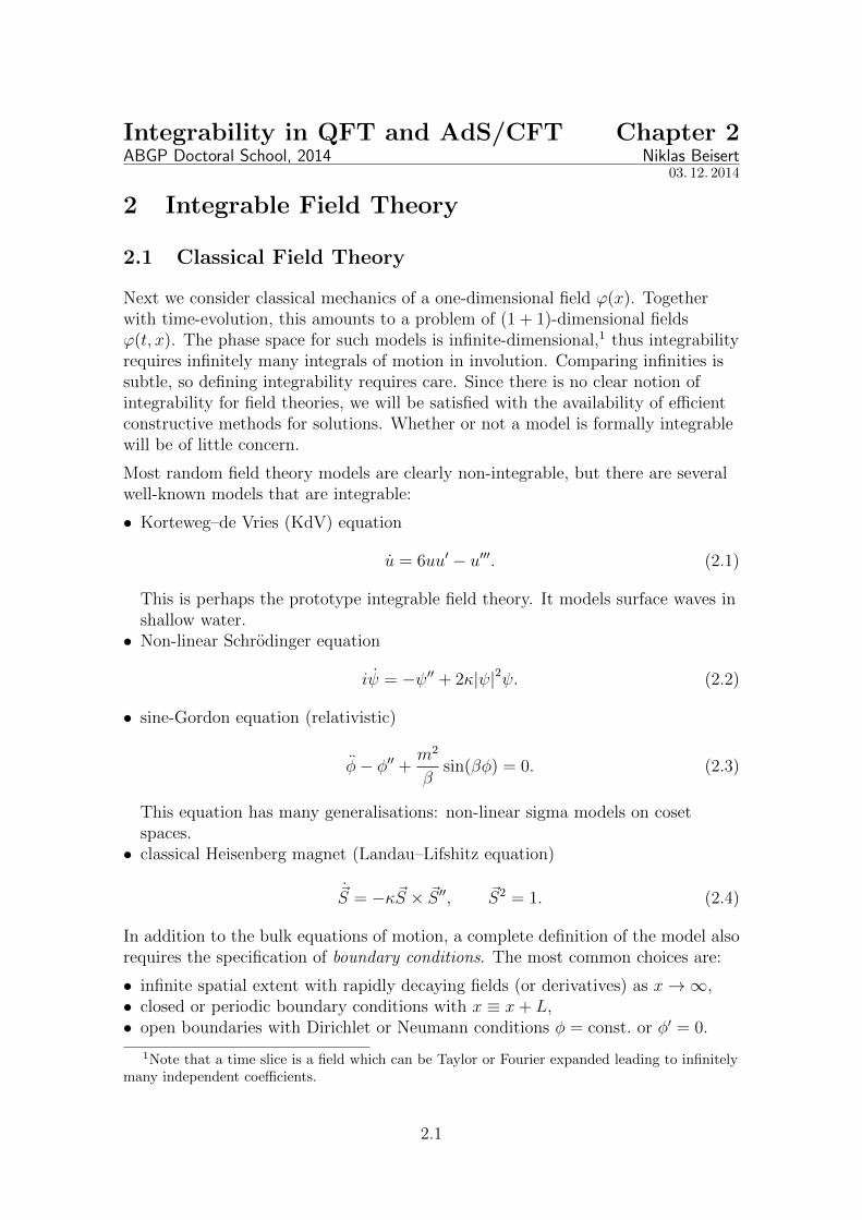
In addition to the bulk equations of motion, a complete definition of the model alsorequires the specification of boundary conditions. The most common choices are:

• infinite spatial extent with rapidly decaying fields (or derivatives) as x→∞,• closed or periodic boundary conditions with x ≡ x+ L,• open boundaries with Dirichlet or Neumann conditions φ = const. or φ′ = 0.

1Note that a time slice is a field which can be Taylor or Fourier expanded leading to infinitelymany independent coefficients.

2.1

x

t

x

t

x

t

(2.5)

Boundary conditions may also be twisted in some way or combined differently.

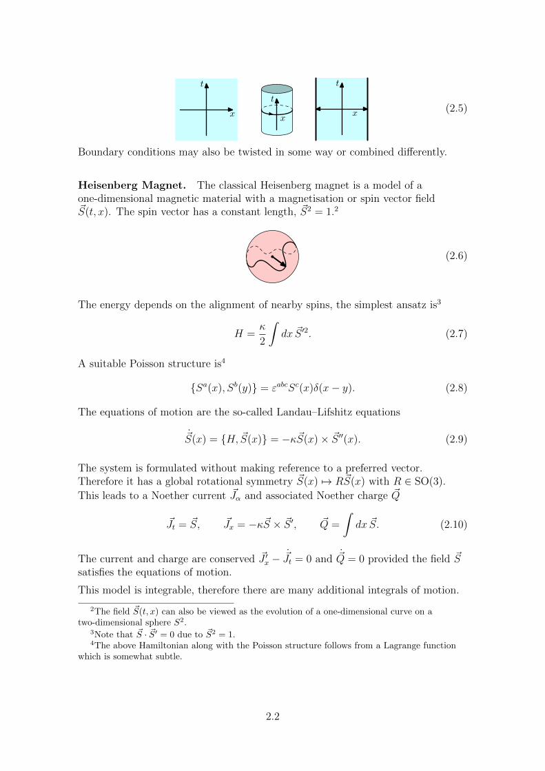
Heisenberg Magnet. The classical Heisenberg magnet is a model of aone-dimensional magnetic material with a magnetisation or spin vector field~S(t, x). The spin vector has a constant length, ~S2 = 1.2

(2.6)

The energy depends on the alignment of nearby spins, the simplest ansatz is3

H =κ

2

∫dx ~S ′2. (2.7)

A suitable Poisson structure is4

{Sa(x), Sb(y)} = εabcSc(x)δ(x− y). (2.8)

The equations of motion are the so-called Landau–Lifshitz equations

~S(x) = {H, ~S(x)} = −κ~S(x)× ~S ′′(x). (2.9)

The system is formulated without making reference to a preferred vector.Therefore it has a global rotational symmetry ~S(x) 7→ R~S(x) with R ∈ SO(3).

This leads to a Noether current ~Jα and associated Noether charge ~Q

~Jt = ~S, ~Jx = −κ~S × ~S ′, ~Q =

∫dx ~S. (2.10)

The current and charge are conserved ~J ′x − ~Jt = 0 and ~Q = 0 provided the field ~Ssatisfies the equations of motion.

This model is integrable, therefore there are many additional integrals of motion.

2The field ~S(t, x) can also be viewed as the evolution of a one-dimensional curve on atwo-dimensional sphere S2.

3Note that ~S · ~S′ = 0 due to ~S2 = 1.4The above Hamiltonian along with the Poisson structure follows from a Lagrange function

which is somewhat subtle.

2.2

Lax Connection. We want to set up a Lax pair to describe the integrals ofmotion for the field theory. In field theory we require infinitely many conservedquantities so the Lax pair has to be infinite-dimensional. Alternatively, we can setup a Lax pair with an additional continuous parameter λ, the so-called spectralparameter. Taylor expansion in λ then leads to an infinite tower of conservedquantities.

Furthermore, the we prefer to formulate in terms of local objects in a field theory.Therefore introduce the Lax connection Aα(λ; t, x)

Ax(λ) = − iλ~σ · ~S,

At(λ) =iκ

λ~σ · (~S × ~S ′) +

2iκ

λ2~σ · ~S. (2.11)

In our case, the Lax connection is a 2× 2 matrix-valued field whose entries dependon λ and are functions of phase space. Here ~σ is the triplet of 2× 2 tracelesshermitian Pauli matrices. The Lax connection satisfies the flatness condition forall λ

Ax(λ)− A′t(λ) + [Ax(λ), At(λ)] = 0 (2.12)

provided that the equations of motion hold and ~S2 = 1.

As always, the Lax connection is not unique. However, a useful recipe to constructit, is to make an ansatz in terms of the components of a Noether current, Jx and Jtin our case, and constrain the coefficients by means of the flatness condition.

It is convenient to work with the Lax connection using the language of differentialforms. It is a su(2) connection one-form A(λ) = Ax(λ)dx+ At(λ)dt which obeysdA(λ) = A(λ) ∧ A(λ).

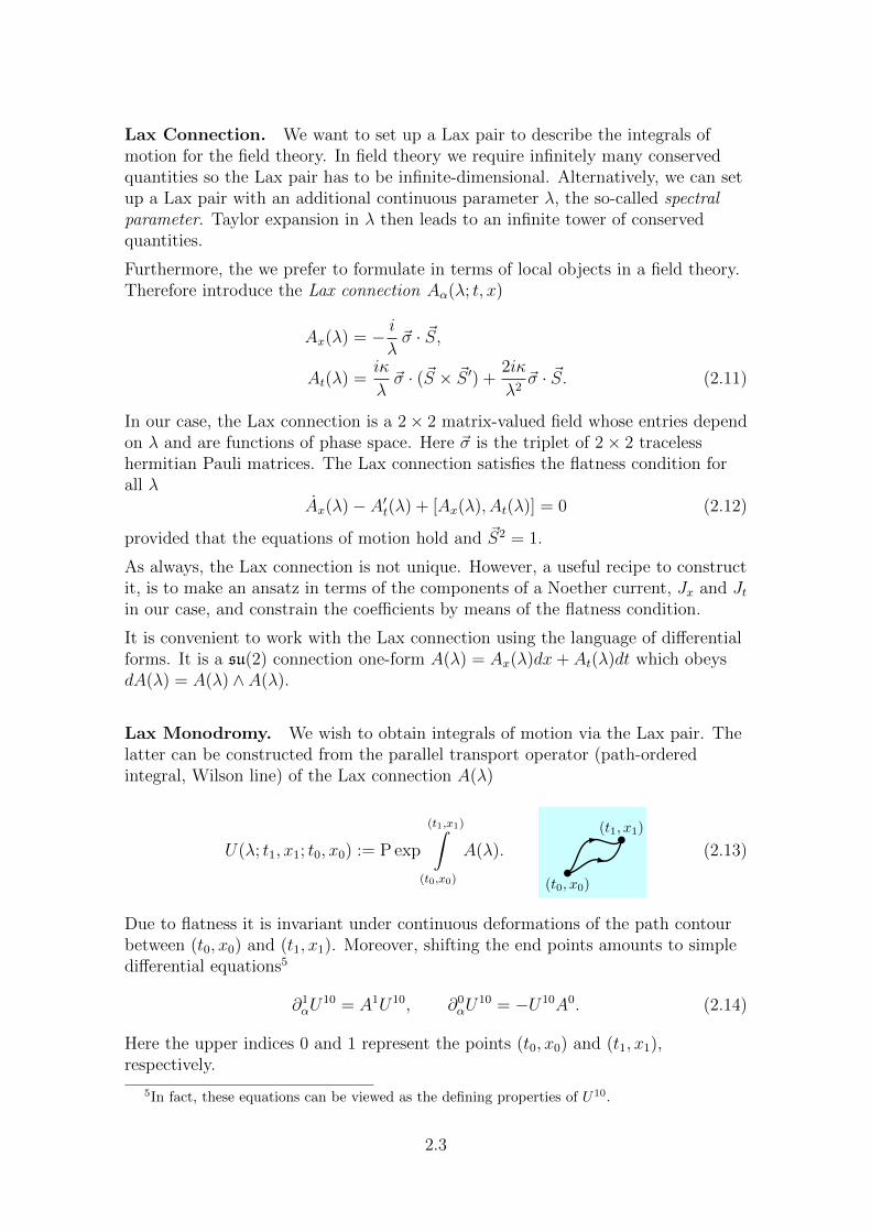
Lax Monodromy. We wish to obtain integrals of motion via the Lax pair. Thelatter can be constructed from the parallel transport operator (path-orderedintegral, Wilson line) of the Lax connection A(λ)

U(λ; t1, x1; t0, x0) := P exp

(t1,x1)∫(t0,x0)

A(λ).

(t0, x0)

(t1, x1)

(2.13)

Due to flatness it is invariant under continuous deformations of the path contourbetween (t0, x0) and (t1, x1). Moreover, shifting the end points amounts to simpledifferential equations5

∂1αU10 = A1U10, ∂0αU

10 = −U10A0. (2.14)

Here the upper indices 0 and 1 represent the points (t0, x0) and (t1, x1),respectively.

5In fact, these equations can be viewed as the defining properties of U10.

2.3

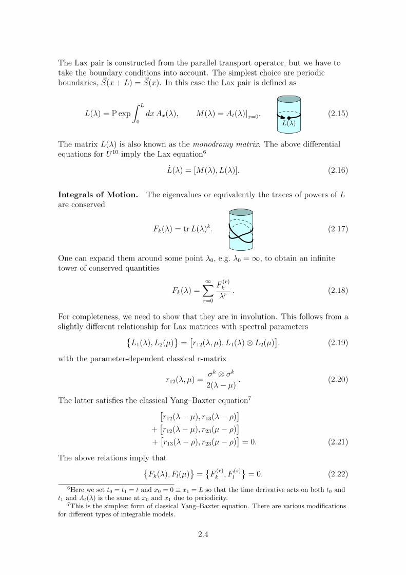
The Lax pair is constructed from the parallel transport operator, but we have totake the boundary conditions into account. The simplest choice are periodicboundaries, ~S(x+ L) = ~S(x). In this case the Lax pair is defined as

L(λ) = P exp

∫ L

0

dxAx(λ), M(λ) = At(λ)|x=0.L(λ)

(2.15)

The matrix L(λ) is also known as the monodromy matrix. The above differentialequations for U10 imply the Lax equation6

L(λ) = [M(λ), L(λ)]. (2.16)

Integrals of Motion. The eigenvalues or equivalently the traces of powers of Lare conserved

Fk(λ) = trL(λ)k. (2.17)

One can expand them around some point λ0, e.g. λ0 =∞, to obtain an infinitetower of conserved quantities

Fk(λ) =∞∑r=0

F(r)k

λr. (2.18)

For completeness, we need to show that they are in involution. This follows from aslightly different relationship for Lax matrices with spectral parameters{

L1(λ), L2(µ)}

=[r12(λ, µ), L1(λ)⊗ L2(µ)

]. (2.19)

with the parameter-dependent classical r-matrix

r12(λ, µ) =σk ⊗ σk

2(λ− µ). (2.20)

The latter satisfies the classical Yang–Baxter equation7[r12(λ− µ), r13(λ− ρ)

]+[r12(λ− µ), r23(µ− ρ)

]+[r13(λ− ρ), r23(µ− ρ)

]= 0. (2.21)

The above relations imply that{Fk(λ), Fl(µ)

}={F

(r)k , F

(s)l

}= 0. (2.22)

6Here we set t0 = t1 = t and x0 = 0 ≡ x1 = L so that the time derivative acts on both t0 andt1 and At(λ) is the same at x0 and x1 due to periodicity.

7This is the simplest form of classical Yang–Baxter equation. There are various modificationsfor different types of integrable models.

2.4

2.2 Spectral Curves

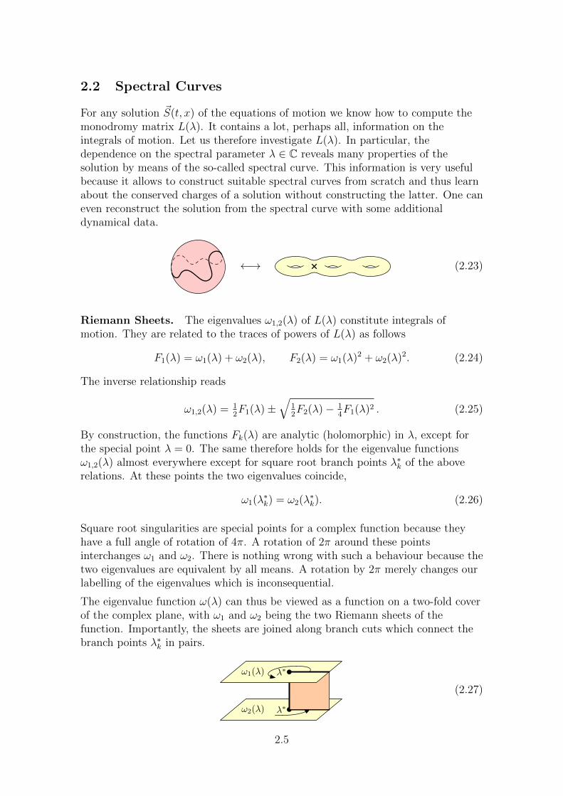
For any solution ~S(t, x) of the equations of motion we know how to compute themonodromy matrix L(λ). It contains a lot, perhaps all, information on theintegrals of motion. Let us therefore investigate L(λ). In particular, thedependence on the spectral parameter λ ∈ C reveals many properties of thesolution by means of the so-called spectral curve. This information is very usefulbecause it allows to construct suitable spectral curves from scratch and thus learnabout the conserved charges of a solution without constructing the latter. One caneven reconstruct the solution from the spectral curve with some additionaldynamical data.

←→ (2.23)

Riemann Sheets. The eigenvalues ω1,2(λ) of L(λ) constitute integrals ofmotion. They are related to the traces of powers of L(λ) as follows

F1(λ) = ω1(λ) + ω2(λ), F2(λ) = ω1(λ)2 + ω2(λ)2. (2.24)

The inverse relationship reads

ω1,2(λ) = 12F1(λ)±

√12F2(λ)− 1

4F1(λ)2 . (2.25)

By construction, the functions Fk(λ) are analytic (holomorphic) in λ, except forthe special point λ = 0. The same therefore holds for the eigenvalue functionsω1,2(λ) almost everywhere except for square root branch points λ∗k of the aboverelations. At these points the two eigenvalues coincide,

ω1(λ∗k) = ω2(λ

∗k). (2.26)

Square root singularities are special points for a complex function because theyhave a full angle of rotation of 4π. A rotation of 2π around these pointsinterchanges ω1 and ω2. There is nothing wrong with such a behaviour because thetwo eigenvalues are equivalent by all means. A rotation by 2π merely changes ourlabelling of the eigenvalues which is inconsequential.

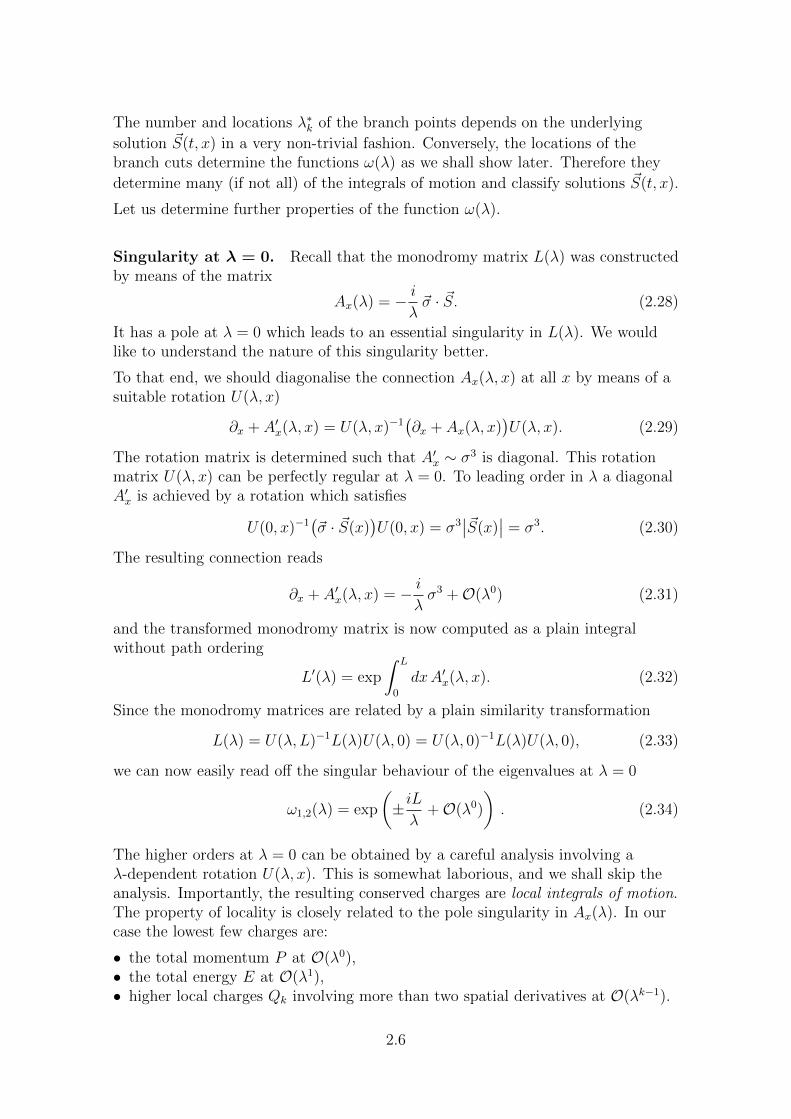
The eigenvalue function ω(λ) can thus be viewed as a function on a two-fold coverof the complex plane, with ω1 and ω2 being the two Riemann sheets of thefunction. Importantly, the sheets are joined along branch cuts which connect thebranch points λ∗k in pairs.

ω2(λ) λ∗

ω1(λ) λ∗

(2.27)

2.5

The number and locations λ∗k of the branch points depends on the underlying

solution ~S(t, x) in a very non-trivial fashion. Conversely, the locations of thebranch cuts determine the functions ω(λ) as we shall show later. Therefore they

determine many (if not all) of the integrals of motion and classify solutions ~S(t, x).

Let us determine further properties of the function ω(λ).

Singularity at λ = 0. Recall that the monodromy matrix L(λ) was constructedby means of the matrix

Ax(λ) = − iλ~σ · ~S. (2.28)

It has a pole at λ = 0 which leads to an essential singularity in L(λ). We wouldlike to understand the nature of this singularity better.

To that end, we should diagonalise the connection Ax(λ, x) at all x by means of asuitable rotation U(λ, x)

∂x + A′x(λ, x) = U(λ, x)−1(∂x + Ax(λ, x)

)U(λ, x). (2.29)

The rotation matrix is determined such that A′x ∼ σ3 is diagonal. This rotationmatrix U(λ, x) can be perfectly regular at λ = 0. To leading order in λ a diagonalA′x is achieved by a rotation which satisfies

U(0, x)−1(~σ · ~S(x)

)U(0, x) = σ3

∣∣~S(x)∣∣ = σ3. (2.30)

The resulting connection reads

∂x + A′x(λ, x) = − iλσ3 +O(λ0) (2.31)

and the transformed monodromy matrix is now computed as a plain integralwithout path ordering

L′(λ) = exp

∫ L

0

dxA′x(λ, x). (2.32)

Since the monodromy matrices are related by a plain similarity transformation

L(λ) = U(λ, L)−1L(λ)U(λ, 0) = U(λ, 0)−1L(λ)U(λ, 0), (2.33)

we can now easily read off the singular behaviour of the eigenvalues at λ = 0

ω1,2(λ) = exp

(±iLλ

+O(λ0)

). (2.34)

The higher orders at λ = 0 can be obtained by a careful analysis involving aλ-dependent rotation U(λ, x). This is somewhat laborious, and we shall skip theanalysis. Importantly, the resulting conserved charges are local integrals of motion.The property of locality is closely related to the pole singularity in Ax(λ). In ourcase the lowest few charges are:

• the total momentum P at O(λ0),• the total energy E at O(λ1),• higher local charges Qk involving more than two spatial derivatives at O(λk−1).

2.6

Quasi-Momentum and Spectral Curve. For a later reconstruction of thefunction ω(λ) the existence of essential singularities is inconvenient. They can beremoved by considering the logarithm of the function ω(λ) which is known as thequasi-momentum q(λ)

q(λ) := −i logω(λ). (2.35)

Evidently, the quasi-momentum has single poles at λ = 0 with residue ±L.

Note that the quasi-momentum q(λ) has inherited the ambiguity of the complexlogarithm, and is therefore defined only modulo shifts of 2π. Evidently, one willchoose the function to be analytic almost everywhere, but in addition to switchingsheets at the existing branch cuts of ω(λ), it can jump by multiples of 2π

q1 ↔ q2 + 2πn. (2.36)

The characteristic number n is constant along the branch cut.

To get rid of these ambiguities, it makes sense to consider the derivative of thequasi-momentum q′ or dq as a differential form,

q′(λ) = −iω′(λ)/ω(λ). (2.37)

This function has only two sheets and algebraic type singularities. It can beviewed as a complex curve, the so-called spectral curve. It is therefore ideallysuited for complex analysis and for construction purposes.

Note that the curve has inherited some properties from its construction via ω(λ).Let us list them:

• All closed periods of dq(λ) on the Riemann surface must be multiples of 2π dueto its definition as a logarithmic derivative∮

dq =

∮dλ q′(λ) ∈ 2πZ. (2.38)

• Any point-like singularities cannot have a residue, i.e. they must be poles ofhigher degree. A pole with a residue requires q(λ) to have a logarithmicsingularity and thus ω(λ) to have a pole or a zero. This is in conflict with thegroup nature of the monodromy L(λ).• There is a double pole at λ = 0 without a residue for the single pole

q′1,2(λ) = ∓ Lλ2

+0

λ+ . . . . (2.39)

• The function q′(λ) has branch cuts which end in inverse square root branchpoints.

Special Properties. The matrix L(λ) has a further special property whichfollows from a property of Ax(λ) and which influences the behaviour of ω(λ) andq(λ).

2.7

We know that Ax ∼ ~σ · ~S in a traceless matrix. After integration andexponentiation we derive

detL(λ) = 1, ω1(λ)ω2(λ) = 1, F2 = F 21 − 2. (2.40)

For the quasi-momentum it implies that the two sheets differ merely by their signand potentially by a shift of a multiple of 2π. In order to fix the shift ambiguity onone sheet, we can define the second sheet to be the negative of the first sheetwithout a shift

q2 = −q1. (2.41)

Passing through a branch cut therefore must include a potential shift by 2π

q ↔ −q + 2πn. (2.42)

Expansion at λ = ∞. Another distinguished point is λ =∞ where Ax(λ)vanishes. The expansion of L(λ) is therefore straight-forwardly the expansion ofthe exponential

L(λ) = exp

(− iλs~σ · ~Q+O(1/λ2)

), (2.43)

where ~Q is the Noether charge for rotations

~Q =

∫ L

0

dx ~Jt, ~Jt = ~S. (2.44)

For the quasi-momentum it implies

q(λ) = ±1

λ| ~Q|. (2.45)

Here we have used and fixed the freedom to shift by multiples of 2π by settingq(∞) = 0.

As an aside, the higher powers of 1/λ in L(λ) correspond to multi-local conservedcharges such as ∫ L

0

dx

∫ x

0

dx′ ~S(x)× ~S(x′). (2.46)

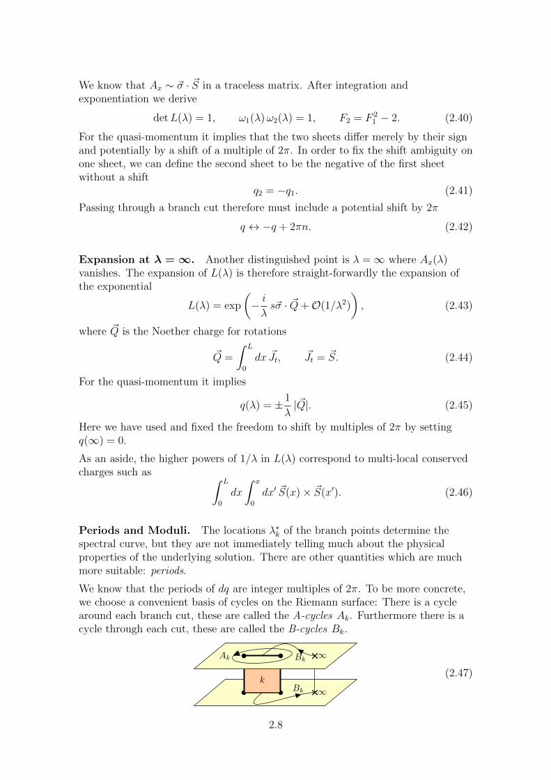
Periods and Moduli. The locations λ∗k of the branch points determine thespectral curve, but they are not immediately telling much about the physicalproperties of the underlying solution. There are other quantities which are muchmore suitable: periods.

We know that the periods of dq are integer multiples of 2π. To be more concrete,we choose a convenient basis of cycles on the Riemann surface: There is a cyclearound each branch cut, these are called the A-cycles Ak. Furthermore there is acycle through each cut, these are called the B-cycles Bk.

∞Bk

k

BkAk ∞

(2.47)

2.8

In this assignment, the distinguished point at λ =∞ can be viewed as aninfinitesimally short cut. It serves as the distinguished cut which does notcontribute to the counting of cycles because

• the combination of all A-cycles combines to an inverse cycle around theremaining singular point λ =∞ and• all B-cycles close though the “cut” at λ =∞.

All A-periods vanish while the B-periods yield integers8∮Ak

dq = 0,

∫Bk

dq = 2πnk. (2.48)

The integers nk describe the jump of the quasi-momentum q(λ) at the branch cuts.They are called mode numbers.

We can measure another characteristic number for each branch cut as the A-periodof λ dq, the so-called filling Kk

Kk =1

2πi

∮Ak

λ dq. (2.49)

It is a measure of the length of the branch cut, and unlike nk it takes continuousvalues. Note that quantisation of the classical theory renders these numbers to bequantised as integers, too.

Finite Gap Construction. Let us summarise the properties of the spectralcurve q′(λ):

• The function has two Riemann sheets, it is single-valued on the Riemannsurface, the sum of the Riemann sheets is zero.• The function has branch points λ∗k of the type 1/

√λ− λ∗k.

• There is a fixed pole ±L/λ2 + 0/λ at λ = 0.• The asymptotic behaviour at λ→ 0 is ∼ 1/λ2.•For spectral curves with finitely many cuts (“finite gap”) we can make a generalansatz as an algebraic curve

q′(λ) = ± PN(λ)

λ2√QN(λ)

, (2.50)

where PN and Q2N are polynomials of degree N and 2N , respectively, with 2N + 2free parameters in total. This ansatz automatically satisfies several of the aboveproperties, the remaining properties constrain some of the parameters as follows:

• N A-periods∮dq = 0,

• N B-periods∫dq = 2πnk,

• N fillings∮λdq ∼ Kk,

8For integer periods one can always make at least half of them vanish by a suitable choice ofindependent cycles and thus of Riemann sheets and cuts.

2.9

• 1 coefficient of the 1/λ2 pole at λ = 0,• 1 ambiguity of overall rescaling of P and

√Q.

We learn that all degrees of freedom are fixed by the knowledge of the (discrete)mode numbers nk and the (continuous) fillings Kk. All integrals of motion(momentum, energy, spin, higher charges) follow from this finite gap solution.

This classifies solutions with finite genus N . One could view the more generalspectral curves with infinitely many cuts as the limiting case N →∞.

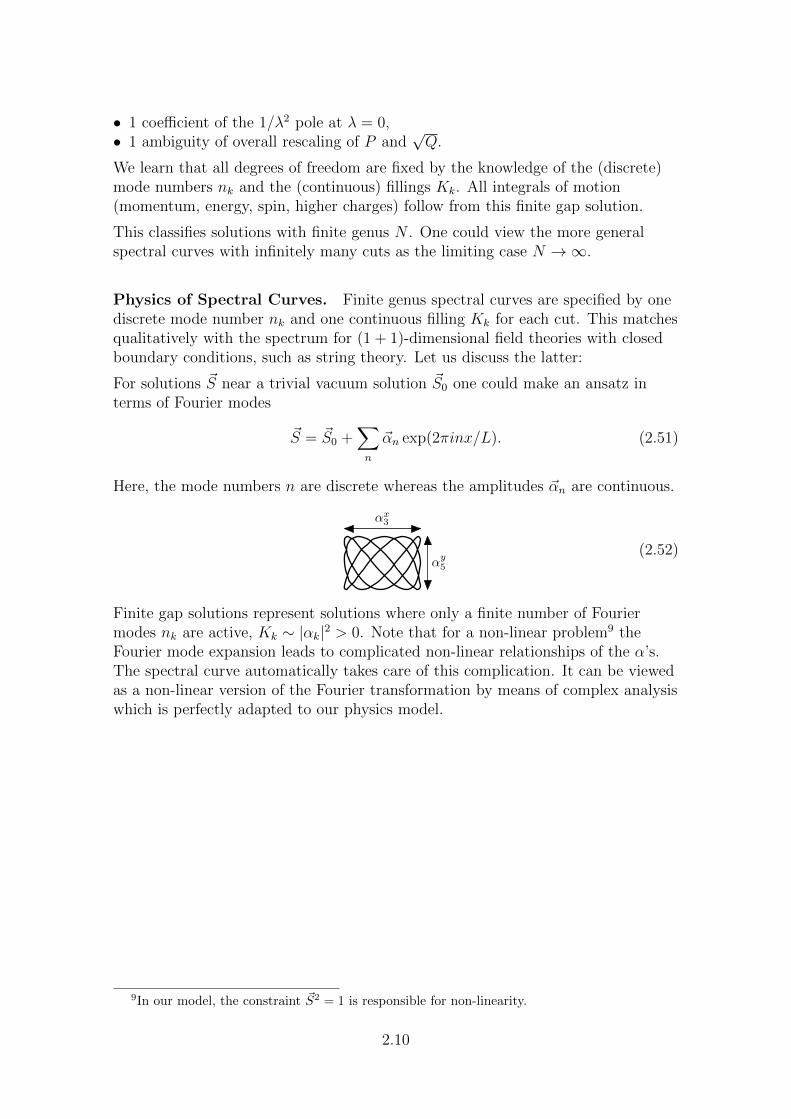
Physics of Spectral Curves. Finite genus spectral curves are specified by onediscrete mode number nk and one continuous filling Kk for each cut. This matchesqualitatively with the spectrum for (1 + 1)-dimensional field theories with closedboundary conditions, such as string theory. Let us discuss the latter:

For solutions ~S near a trivial vacuum solution ~S0 one could make an ansatz interms of Fourier modes

~S = ~S0 +∑n

~αn exp(2πinx/L). (2.51)

Here, the mode numbers n are discrete whereas the amplitudes ~αn are continuous.

αx3

αy5

(2.52)

Finite gap solutions represent solutions where only a finite number of Fouriermodes nk are active, Kk ∼ |αk|2 > 0. Note that for a non-linear problem9 theFourier mode expansion leads to complicated non-linear relationships of the α’s.The spectral curve automatically takes care of this complication. It can be viewedas a non-linear version of the Fourier transformation by means of complex analysiswhich is perfectly adapted to our physics model.

9In our model, the constraint ~S2 = 1 is responsible for non-linearity.

2.10

Integrability in QFT and AdS/CFT Chapter 3ABGP Doctoral School, 2014 Niklas Beisert

10. 12. 2014

3 Integrable Spin Chains

We now proceed to integrable quantum mechanical models. They are instructivebecause:

• they form a large class of integrable models,• they can be treated uniformly,• they have many parameters to tune,• short chains are genuine quantum mechanical models,• long chains approximate (1 + 1)D quantum field theories,• for large quantum numbers they are approximated by classical models,• they model magnetic materials.

Magnets. Ansatz: A magnetic material consists of many microscopic magnets,e.g. atoms with spin. The energy of the material depends on the configuration ofnearby spins.

nearby spins ferromagnet anti-ferromagnetopposite alignment ↑↓ high energy low energy

equal alignment ↑↑ low energy high energy(3.1)

Two well known models of magnets are:

• Ising model, a model of statistical mechanics. It consists of a lattice of spinstaking values ↑, ↓. The alignment of nearest neighbours determines the energy.• Heisenberg chain, a quantum mechanical model. It consists of a chain of spin

states |↑〉, |↓〉. The Hamiltonian acts on nearest neighbours.

In the following we shall discuss the Heisenberg spin chain in detail.

3.1 Heisenberg Spin Chain

Let us start by introducing the model and investigating its spectrum.

Setup. A single spin state can be |↓〉 or |↑〉 or any complex linear combination ofthese two. In other words, a spin is described by an element of the vector space

V = C2. (3.2)

A spin chain of length L is the L-fold tensor product

V⊗L = V1 ⊗ . . .⊗ VL. (3.3)

This space serves as the Hilbert space of our model. It has finite dimension 2L. Abasis is given by the “pure” states, e.g.

|↑↑↓↑↑↑↑↓〉. (3.4)

3.1

The Hamiltonian operator H : V⊗L → V⊗L is homogeneous and acts on nearestneighbours

H =∑

kHk,k+1, Hk,l : Vk ⊗ Vl → Vk ⊗ Vl. (3.5)

The pairwise kernel Hk,l for the Heisenberg chain reads

Hk,l = λ0(1⊗ 1) + λx(σx ⊗ σx) + λy(σ

y ⊗ σy) + λz(σz ⊗ σz). (3.6)

It is integrable for all values of the coupling constants λ0, λx, λy, λz. Several usefulcases can be distinguished:

• The most general (and most complicated) case is λx 6= λy 6= λz 6= λx: This is theso-called “XYZ” model.• Many simplifications occur for λx = λy 6= λz: This is the so-called “XXZ” model.• Symmetry is enhanced for λx = λy = λz: This is the so-called “XXX” model.

We shall mainly use the XXX model with the choice1

λ0 = −λx = −λy = −λz = 12λ. (3.7)

With this choice the Hamiltonian kernel reads

Hk,l = λ(Ik,l − Pk,l), (3.8)

where Ik,l is the identity operator and Pk,l the permutation on the two equivalentspaces Vk and Vl. Note that λ > 0 implies ferromagnetic behaviour whereas λ < 0implies anti-ferromagnetic behaviour.2

Boundary Conditions. To complete the definition of the model, we mustspecify the boundary conditions. Typical choices are

• open chain:

H =L−1∑k=1

Hk,k+1, (3.9)

• closed chain: identify sites periodically such that VL+1 = V1

H =L∑k=1

Hk,k+1, (3.10)

• infinite chain:

H =+∞∑

k=−∞

Hk,k+1. (3.11)

1The value of λ0 is largely irrelevant because it merely induces an overall shift of all energies.Our choice sets the energy of a reference state to zero.

2We shall be interested in all states of the model, hence the difference between theferromagnetic and anti-ferromagnetic case is merely an overall sign of the energy spectrum. Thedistinction between the two cases becomes relevant only when considering the ground state andits low-energy excitations.

3.2

Other choices that are sometimes encountered include:

• twists of the closed boundary conditions,• open boundary conditions with specific boundary Hamiltonians,• semi-infinite chains.

Some of these boundary conditions are compatible with integrability, others maynot.

Boundary conditions have a strong impact on the spectrum: Infinite chainsgenerally have a continuous spectrum while finite chains by have a discretespectrum by definition. This makes the spectral problem more interesting for finitechains. Here, the closed chains are typically easier to handle than open chains,therefore we shall mainly consider the former.

Spectrum. Consider a finite chain, how to obtain the spectrum?

• Enumerate a basis of V⊗L, e.g. |↓ . . . ↓↓〉, |↓ . . . ↓↑〉, . . . amounting to 2L states intotal.• Evaluate H in this basis as a 2L × 2L matrix. This uninspiring task of basic

combinatorics leads to a sparse matrix of integer entries.• Next solve the eigenvalue problem of the Hamiltonian matrix.

The problem is ideally suited for computer algebra:

• One can automatically evaluate the Hamiltonian as a matrix for fairly large L.• An exact diagonalisation in terms of algebraic numbers if feasible only for smallL.• Numerical evaluation of the eigenvalues allows slightly larger values of L.• The spectrum is a big mess.• Eigenvalues appear in multiplets.

Spectrum in Mathematica. Let us present a concise implementation of theXXX Hamiltonian in Mathematica.

First, we need to find a way to represent spin chain states. An immediate thoughtwould be to define them as vectors with 2L components. A drawback of thisapproach is that one obtains rather abstract and obscure objects which growexponentially fast with L and which are not so easy to act upon. An alternativeand more symbolic approach is to “define” a set of abstract basis vectors and allowfor linear combinations. For example, we can represent pure spin chain states byfunctions whose arguments denote the spin orientations

|↑, ↑, ↓, ↑, ↓〉 → State[1,1,0,1,0]. (3.12)

The function State is undefined by default, so it remains unevaluated and can beused to represent linear combinations, e.g.

10 State[1,1,0,1,0]− 5 State[1,0,1,1,0]. (3.13)

Next we have to represent the Hamiltonian H through some replacement operator

Ham :∑∗State[...]→

∑∗State[...]. (3.14)

3.3

A homogeneous nearest neighbour Hamiltonian can be implemented by thefollowing code:

Ham[X_] :=

X /. Psi_State :> Module[{k, L=Length[Psi]},

Sum[HamAt[Psi, k, Mod[k+1, L, 1]],

{k, L}]];

(3.15)

This function replaces (/., ReplaceAll) every occurrence of State in theargument X with the homogeneous action of the kernel HamAt. Some notes:

• Psi_State symbolises any object State[...], i.e. any object with head State.3

• The use of the replacement operator :> (RuleDelayed) as opposed to -> (Rule)is essential because it evaluates the right hand side only after insertion of Psi.• The above definition assumes that the argument X is a linear combination ofState objects. If X is not a linear combination of State objects, Ham doeswhatever it does (replace objects). Lists, vectors, matrices, nested lists of linearcombinations of State objects are permissible as arguments: Ham will act oneach element individually.• The construct Module defines a local variable k 4 and a local variable L assigned

with the length of the state Psi.

The Hamiltonian kernel for the XXX model can be defined as

HamAt[Psi_State, k_, l_] :=

Psi - Permute[Psi, Cycles[{{k,l}}]];(3.16)

It uses some pre-defined combinatorial methods to implement the permutation oftwo sites in the symbol Psi.

We are now ready to act on states. In order to obtain the complete spectrum wehave to enumerate a basis of V⊗L. As a shortcut, we can employ the binaryrepresentation of integers 0, . . . , 2L − 1:

Basis[L_] :=

Table[State @@ IntegerDigits[k, 2, L],

{k, 0, 2^L-1}];

(3.17)

Here the operator @@ (Apply) replaces the head of the binary representation of k(which is List) with State. The variable states is now a list of pure basis states.

To evaluate the Hamiltonian on the states we can use the following construct:

HamMat[states_] :=

Module[{X=Ham[states]},

Coefficient[X, #] & /@ states];

(3.18)

Some notes:3Almost all objects in Mathematica (except variables and concrete numbers) are headed lists.

They can be treated much like lists (which are in fact objects with head List).4Sometimes using the same variable names as arguments of a Sum and elsewhere can lead to

undesired interference (depending on the order of evaluation of sub-expressions). To avoid apotential interference it makes sense to make the summation variable local.

3.4

• Ham[states] evaluates Ham on every element of the list states. Usually, onewould have to explicitly declare this behaviour for the function Ham by means ofSetAttributes[Ham, Listable]. In our case, the definition via a replacementrule automatically implements this desired behaviour.• The operator & (Function) represents a pure function (a function without a

declaration) which returns Coefficient[X, #] where # is the argument passedto the function. In practice it extracts the coefficient of the argument within X.• The operator /@ (Map) evaluates the above pure function on all elements of the

list states. This is the matrix representation of Ham in the basis states.5

To finally extract the eigenvalues, generate the Hamiltonian matrix via (rememberto substitute or define L as a not too large positive integer)

emat = HamMat[Basis[L]]; (3.19)

and use Eigenvalues[emat], Eigenvalues[N[emat]] orEigenvalues[N[emat, 20]].

Symmetry. The XXX Hamiltonian has a SU(2) Lie group symmetry becausethe kernel Hk,l is formulated as a manifestly SU(2) invariant operator.

We can set up a representation J α, α = x, y, z, of the Lie algebra su(2) on spinchains

J α =L∑k=1

σαk . (3.20)

• This is a tensor product representation of L spin 1/2 irreps of su(2) given by thePauli matrices σαk acting on site k.• The Hamiltonian is invariant

[J α,H] = 0. (3.21)

• The tensor product is decomposable, for the shortest few chains one finds by thewell-known tensor product rules for su(2):

L = 2 : (1) + (0);L = 3 : (3

2) + 2(1

2);

L = 4 : (2) + 3(1) + 2(0);L = 5 : (5

2) + 4(3

2) + 5(1

2);

L = 6 : (3) + 5(2) + 9(1) + 5(0);. . . .

(3.22)

Here (s) denotes a finite irrep of spin s.• Each multiplet has one common eigenvalue.

The spectrum of the closed chain of small length L in units of λ takes a fairly

5Potentially, one should Transpose the matrix.

3.5

simple form:

L eigenvalue multiplets

2 (1)× 0, (0)× 4;3 (3

2)× 0, 2(1

2)× 3;

4 (2)× 0, 2(1)× 2, (1)× 4,(0)× 6, (0)× 2;

5 (52)× 0, 2(3

2)× 1

2(5 +

√5), 2(3

2)× 1

2(5−

√5),

(12)× 4, 2(1

2)× 4 +

√5, 2(1

2)× 4−

√5;

6 (3)× 0, 2(2)× 3, 2(2)× 1,

(2)× 4, 2(1)× 12(7 +

√17), 2(1)× 1

2(7−

√17),

2(1)× 5, (1)× 5 +√

5, (1)× 5−√

5,

(1)× 2, (0)× 5 +√

13, (0)× 5−√

13,2(0)× 4, (0)× 6;. . . .

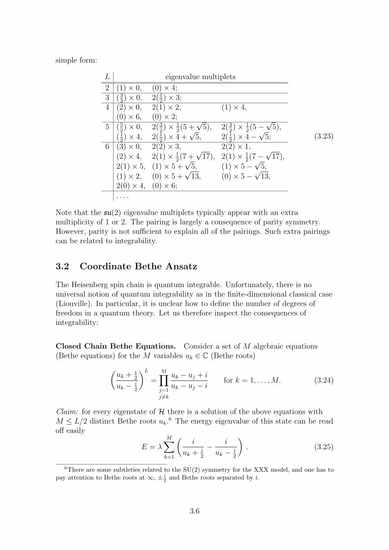
(3.23)

Note that the su(2) eigenvalue multiplets typically appear with an extramultiplicity of 1 or 2. The pairing is largely a consequence of parity symmetry.However, parity is not sufficient to explain all of the pairings. Such extra pairingscan be related to integrability.

3.2 Coordinate Bethe Ansatz

The Heisenberg spin chain is quantum integrable. Unfortunately, there is nouniversal notion of quantum integrability as in the finite-dimensional classical case(Liouville). In particular, it is unclear how to define the number of degrees offreedom in a quantum theory. Let us therefore inspect the consequences ofintegrability:

Closed Chain Bethe Equations. Consider a set of M algebraic equations(Bethe equations) for the M variables uk ∈ C (Bethe roots)(

uk + i2

uk − i2

)L=

M∏j=1

j 6=k

uk − uj + i

uk − uj − ifor k = 1, . . . ,M. (3.24)

Claim: for every eigenstate of H there is a solution of the above equations withM ≤ L/2 distinct Bethe roots uk.

6 The energy eigenvalue of this state can be readoff easily

E = λM∑k=1

(i

uk + i2

− i

uk − i2

). (3.25)

6There are some subtleties related to the SU(2) symmetry for the XXX model, and one has topay attention to Bethe roots at ∞, ± i

2 and Bethe roots separated by i.

3.6

Example: L = 6, M = 3 (corresponding to a spin singlet)

u1,2 = ±

√− 5

12+

√13

6, u3 = 0, E = λ(5 +

√13). (3.26)

Benefits:

• We have transformed a problem of linear algebra directly to algebraic equations.We can thus skip combinatorics and characteristic polynomials.• We can use the Bethe equations efficiently for approximations at large L and M .

For example, the anti-ferromagnetic ground state can be approximated at largeL in which case the Bethe equations turn into integral equations.

In the following we shall derive the Bethe equations from the coordinate Betheansatz.

Vacuum State. Start with a simple state, the ferromagnetic vacuum

|0〉 = |↓↓ . . . ↓〉. (3.27)

By construction this state has zero energy

Hk,k+1|0〉 = Ik,k+1|0〉 − Pk,k+1|0〉 = |0〉 − |0〉 = 0. (3.28)

Therefore H|0〉 = 0 and the ground state energy is zero

E = 0. (3.29)

This solves the problem for M = 0 corresponding to the multiplet (L/2).

Magnon States. Now flip one spin at site k

|k〉 = |↓ . . . ↓k

↑↓ . . . ↓〉. (3.30)

These states enumerated by k form a closed sector under the Hamiltonian due toconservation of the z-component of spin J z.

How to obtain eigenstates of H? Note that the Hamiltonian is homogeneous andcommutes with a shift of the chain by one unit.7 We can thus look forsimultaneous eigenstates of the Hamiltonian and the shift operator. Momentumeigenstates are plane waves8

|p〉 =∑

keipk|k〉. (3.31)

This state is called a magnon state. It can be viewed as a particle excitation9 ofthe above vacuum state.

7The lattice shift is a discrete version of the momentum generator.8The notation is slightly ambiguous, but it should become clear from the context whether |∗〉

refers to a position eigenstate |k〉 or a momentum eigenstate |p〉.9Here the notion of particle is an object which carries an individual momentum p.

3.7

Since there is a unique state with a given momentum p, it must already by anenergy eigenstate. We can now act with H on |p〉 and obtain (after a shift ofsummation variable to match the states on the r.h.s.)

H|p〉 = λ∑

keipk( Hk−1,k︷ ︸︸ ︷|k〉 − |k − 1〉+

Hk,k+1︷ ︸︸ ︷|k〉 − |k + 1〉

)= λ

∑keipk(1− eip + 1− e−ip

)|k〉

= e(p)|p〉 (3.32)

with the magnon dispersion relation

e(p) = 2λ(1− cos p) = 4λ sin2(12p). (3.33)

For a closed chain, the momentum is quantised by the periodic boundaryconditions to

p =2πin

L, where n = 0, . . . , L− 1. (3.34)

For an infinite chain p is a continuous parameter. Note that in both cases themomentum is defined only modulo 2π because the position k is sampled only atthe discrete lattice positions. A shift by 2π corresponds to a change of Brillouinzone which leaved the eigenstate unchanged.

This solves the problem for M = 1 corresponding to the multiplets (L/2− 1).10

Scattering Factor. We continue with states with two spin flips

|k < l〉 = |↓ . . . ↓k

↑↓ . . . ↓l

↑↓ . . . ↓〉. (3.35)

Here we make the assumption that k < l. Again, these states form a closed sectorfor the Hamiltonian, and we wish to construct eigenstates.

When the spin flips are well-separated we can treat the state as the combination oftwo individual magnons. The nearest neighbour Hamiltonian will hardly every seeboth spin flips at the same time, therefore we can make an ansatz for eigenstatesof the form

|p < q〉 =+∞∑

k<l=−∞

eipk+iql|k < l〉. (3.36)

Some comments:

• This state has overall momentum P = p+ q.• The momenta of the individual spin flips are not well-defined because their wave

functions do not extend over the whole chain, but are constrained by an orderingof the spin flips. Nevertheless we can use p and q as labels for a particular state.• The notation |p < q〉 is not meant to imply that p is less than q, but rather that

the magnon with momentum p is to the right of the magnon with momentum q.

10The state with p = 0 belongs to the multiplet (L/2) discussed in the context of the vacuum.

3.8

• For the time being we shall only consider an infinite chain so that we do nothave to worry about boundary conditions.

By construction, each of these states is almost an eigenstate with eigenvalue

E = e(p) + e(q). (3.37)

Acting with the combination H− e(p)− e(q) on |p < q〉 yields

(eip+iq − 2eiq + 1

) +∞∑k=−∞

ei(p+q)k|k < k + 1〉. (3.38)

Only a contact term∑

k ei(p+q)k|k < k + 1〉 remains and violates the eigenstate

condition. Since this state is symmetric in p and q we can act on the state |q < p〉with the magnon momenta interchanged and obtain a proportional term

(eip+iq − 2eip + 1

) +∞∑k=−∞

ei(p+q)k|k < k + 1〉. (3.39)

We can now patch together the two partial wave functions and construct an exacteigenstate11

|p, q〉 = |p < q〉+ S(p, q)|q < p〉 (3.40)

with a scattering factor S

S(p, q) = −eip+iq − 2eiq + 1

eip+iq − 2eip + 1.

p q

pqS (3.41)

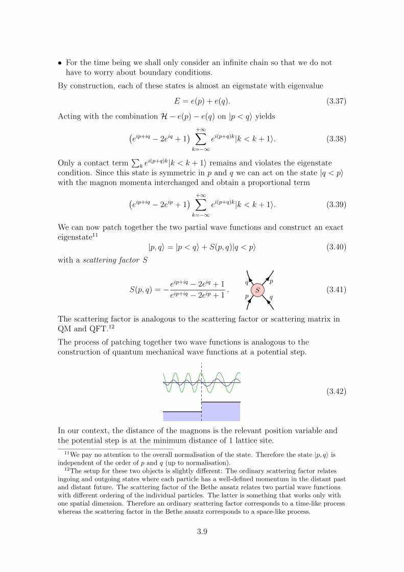
The scattering factor is analogous to the scattering factor or scattering matrix inQM and QFT.12

The process of patching together two wave functions is analogous to theconstruction of quantum mechanical wave functions at a potential step.

(3.42)

In our context, the distance of the magnons is the relevant position variable andthe potential step is at the minimum distance of 1 lattice site.

11We pay no attention to the overall normalisation of the state. Therefore the state |p, q〉 isindependent of the order of p and q (up to normalisation).

12The setup for these two objects is slightly different: The ordinary scattering factor relatesingoing and outgoing states where each particle has a well-defined momentum in the distant pastand distant future. The scattering factor of the Bethe ansatz relates two partial wave functionswith different ordering of the individual particles. The latter is something that works only withone spatial dimension. Therefore an ordinary scattering factor corresponds to a time-like processwhereas the scattering factor in the Bethe ansatz corresponds to a space-like process.

3.9

Factorised Scattering. Before considering closed chains, let us have a look atthree-magnon states. There are 6 = 3! asymptotic regions for magnons which carryone momentum pk each. A useful ansatz for an eigenstate is the so-called Betheansatz

|p1, p2, p3〉 = |p1 < p2 < p3〉+ S12S13S23|p3 < p2 < p1〉+ S12|p2 < p1 < p3〉+ S13S23|p3 < p1 < p2〉+ S23|p1 < p3 < p2〉+ S12S13|p2 < p3 < p1〉. (3.43)

All pairwise contact terms vanish by construction due to the choice of appropriatepairwise scattering factors between any two partial wave functions. There could inprinciple be a triple contact term(

H− E)|p1, p2, p3〉 ∼

∑keiPk|k < k + 1 < k + 2〉. (3.44)

Due to a miracle this contact term is absent without further ado. This miracle iscalled integrability.13 It works analogously for any number of magnons as we shalldiscuss below. We only need the two-magnon scattering factor to constructarbitrary states.

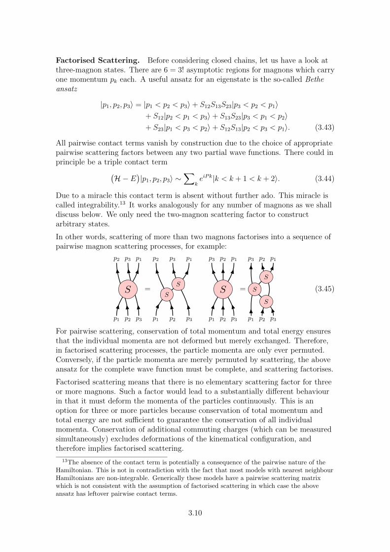
In other words, scattering of more than two magnons factorises into a sequence ofpairwise magnon scattering processes, for example:

p1 p2 p3

p1p2 p3

S =

p1 p2 p3

p1p2 p3

S

S

p1 p2 p3

p1p2p3

S =

p1 p2 p3

p1p2p3

S

S

S

(3.45)

For pairwise scattering, conservation of total momentum and total energy ensuresthat the individual momenta are not deformed but merely exchanged. Therefore,in factorised scattering processes, the particle momenta are only ever permuted.Conversely, if the particle momenta are merely permuted by scattering, the aboveansatz for the complete wave function must be complete, and scattering factorises.

Factorised scattering means that there is no elementary scattering factor for threeor more magnons. Such a factor would lead to a substantially different behaviourin that it must deform the momenta of the particles continuously. This is anoption for three or more particles because conservation of total momentum andtotal energy are not sufficient to guarantee the conservation of all individualmomenta. Conservation of additional commuting charges (which can be measuredsimultaneously) excludes deformations of the kinematical configuration, andtherefore implies factorised scattering.

13The absence of the contact term is potentially a consequence of the pairwise nature of theHamiltonian. This is not in contradiction with the fact that most models with nearest neighbourHamiltonians are non-integrable. Generically these models have a pairwise scattering matrixwhich is not consistent with the assumption of factorised scattering in which case the aboveansatz has leftover pairwise contact terms.

3.10

Solution of the Infinite Chain. We have found an explicit and exact solutionfor the eigenstates of the infinite chain with an arbitrary number of magnons.

|0〉 = |↓ . . . ↓〉, E = 0,

|p〉 =∑

keipk|. . .

k

↑ . . .〉, E = e(p),

|p, q〉 = |p < q〉+ S(p, q)|q < p〉, E = e(p) + e(q),

|pk〉 =∑π∈SM

Sπ|pπ(1) < . . . < pπ(M)〉, E =∑k

e(pk) (3.46)

The momenta pk are arbitrary numbers, therefore the spectrum is continuous.

Note:

• The ordering of the pk does not matter: magnons are identical particles.• The momenta pk are defined modulo 2π: they move on a lattice.• The momenta should be real for wave functions to be normalisable (in the

ordinary sense of plane waves).• For two identical momenta

S(p, p) = −1 =⇒ |p, p, . . .〉 = 0. (3.47)

The value of the scattering factor and the exclusion principle indicates that theparticles obey Fermi statistics. The XXX model on the infinite chain isequivalent to free fermions on a one-dimensional lattice!• Zero-momentum particles are special:

S(p, 0) = 1, e(0) = 0. (3.48)

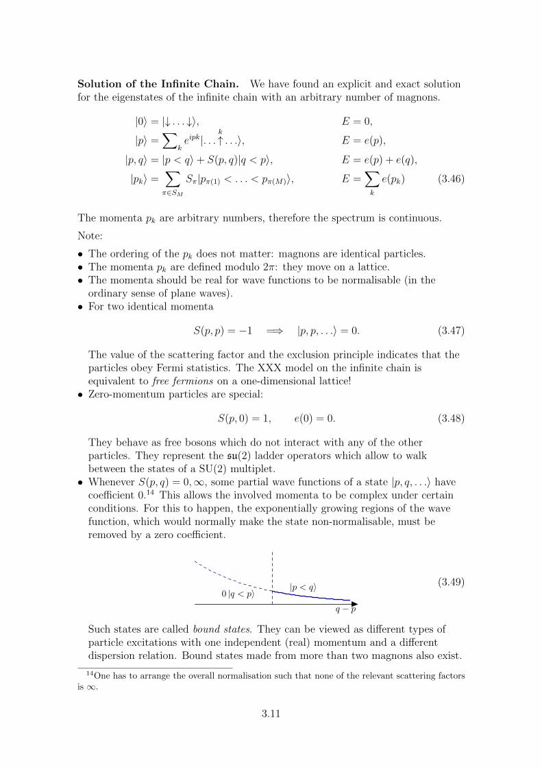
They behave as free bosons which do not interact with any of the otherparticles. They represent the su(2) ladder operators which allow to walkbetween the states of a SU(2) multiplet.• Whenever S(p, q) = 0,∞, some partial wave functions of a state |p, q, . . .〉 have

coefficient 0.14 This allows the involved momenta to be complex under certainconditions. For this to happen, the exponentially growing regions of the wavefunction, which would normally make the state non-normalisable, must beremoved by a zero coefficient.

q − p

|p < q〉0 |q < p〉

(3.49)

Such states are called bound states. They can be viewed as different types ofparticle excitations with one independent (real) momentum and a differentdispersion relation. Bound states made from more than two magnons also exist.

14One has to arrange the overall normalisation such that none of the relevant scattering factorsis ∞.

3.11

Periodicity and Bethe Equations. We know how to solve the infinite XXXchain, but we would like to understand the spectrum of the finite closed chain. Tothis end, we can compare states of the closed chain with periodic states of theinfinite chain. There are at least two conceivable notions of periodic states:

• states with periodic excitations

|. . . , k1 − L, k1, k1 + L, . . . , k2 − L, k2, k2 + L, . . .〉. (3.50)

• states with a periodic wave function

〈k, . . . |Ψ〉 = 〈k + L, . . . |Ψ〉. (3.51)

The advantage of the latter point of view is that it requires only finitely manyexcitations. Let us therefore continue along these lines:

• Consider a position space configuration where the magnons are separated by lessthan L sites.15

• Focus on the leftmost excitation and pay attention to how the wave function ofan eigenstate evolves as this excitation is shifted towards the right.• Moving the excitation by L sites generates a factor of eipkL by construction.• Along the way, it will move past all the other excitations and pick up a factor ofS(pk, pj) for each permutation.16

• The eigenstate is periodic if all the phase factors multiply to 1.• Such a periodic wave function can be lifted to the wave function on a closed

chain.17

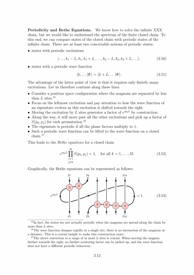
This leads to the Bethe equations for a closed chain

eipkLM∏j=1

j 6=k

S(pk, pj) = 1, for all k = 1, . . . ,M. (3.52)

Graphically, the Bethe equations can be represented as follows:

eipkL

S S

S S S S

p1 pk pM

p1 pk pM

= 1. (3.53)

15In fact, the states are not actually periodic when the magnons are spread along the chain bymore than L sites.

16The wave function changes rapidly at a single site, there is no interaction of the magnons ata distance. This is a crucial insight to make this construction exact.

17The above restriction to a range of at most L sites is crucial. When moving the magnonfurther towards the right, no further scattering factor can be picked up, and the wave functiondoes not have a different periodic behaviour.

3.12

They amount to one equation for each unknown variable pk. This effectivelyquantises the spectrum. A simple consistency requirement for the closed chainalready leads to a discrete set of solutions.

The total energy and total momentum of a solution can be read off from the set ofmagnon momenta pk

E =M∑k=1

e(pk), P =M∑k=1

pk. (3.54)

One can simply derive a useful statement on P by multiplying all Bethe equations,namely

eiPL = 1. (3.55)

This relationship follows from triviality of an overall shift by L sites where eiP isthe eigenvalue of the cyclic shift operator.

Rapidities. It is convenient to introduce a different set of variables uk instead ofthe momenta pk.

pk = 2 arccot 2uk, uk = 12

cot 12pk. (3.56)

The scattering factor simplifies to a rational function

S(u, v) =u− v − iu− v + i

. (3.57)

The Bethe equations then take the form introduced earlier(uk + i

2

uk − i2

)L=

M∏j=1

j 6=k

uk − uj + i

uk − uj − ifor k = 1, . . . ,M. (3.58)

and the energy and momentum eigenvalues are obtained via

eiP =M∏k=1

uk + i2

uk − i2

, E = λM∑k=1

(i

uk + i2

− i

uk − i2

). (3.59)

Let us mention some special points and configurations:

• The uk are real or form complex conjugate pairs.18

• All uk must be distinct except for the special value uk =∞ which can appearseveral times.• The su(2) ladder operators at pk = 0 correspond to uk =∞.• The special values uk = ± i

2where pk =∞ which typically do not appear in

physically relevant solutions. However, some relevant singular solutions exist.• There is no analog of the periodicity of the pk for the uk.• We should restrict to M ≤ 1

2L; the other states with M > 1

2L are represented

via a collection of uk =∞ added to a solution with M ≤ 12L.

• Bound states with S(uk, uj) = 0,∞ are obtained for the simple conditionuk = uj ± i. Higher bound states correspond to so-called Bethe stringsuk = u0 + ik.

18Normalisability is not an issue for finite chains.

3.13

3.3 Generalisation

Open Chains. Consider an open chain with Hamiltonian

H =L−1∑k=1

Hk,k+1. (3.60)

To quantify the effect of the boundaries, consider a semi-infinite chain starting atsite k = 1. Act with H− e(p) on a one-magnon state |+p〉.(

H− e(p))|+p〉 = (1− e+ip)|1〉. (3.61)

As for the two-magnon state, there is a residual term located at the boundary.This term can be compensated by another partial eigenstate with equal energye(p) = e(p), namely p = −p.(

H− e(p))|−p〉 = (1− e−ip)|1〉. (3.62)

Now combine the states into an exact eigenstate19 20

|p〉 = e−ip|+p〉+ e+ipKL(−p)|−p〉 (3.63)

with the boundary scattering factor

KL(−p) = −e−2ip1− e+ip

1− e−ip= e−ip. (3.64)

Similarly, one can construct exact eigenstates for a semi-infinite chain ending atsite k = L

|p〉 = e−ipL|+p〉+ e+ipLKR(+p)|−p〉 (3.65)

with boundary scattering factor

KR(+p) = e+ip. (3.66)

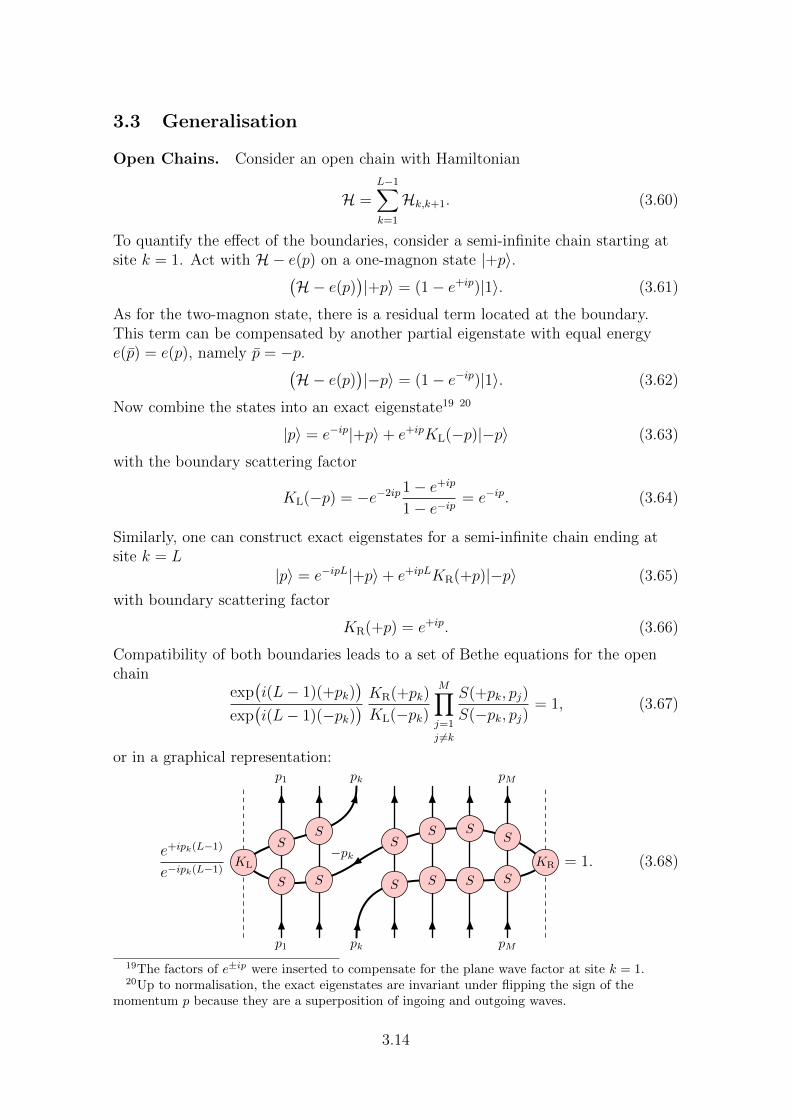
Compatibility of both boundaries leads to a set of Bethe equations for the openchain

exp(i(L− 1)(+pk)

)exp(i(L− 1)(−pk)

) KR(+pk)

KL(−pk)

M∏j=1

j 6=k

S(+pk, pj)

S(−pk, pj)= 1, (3.67)

or in a graphical representation:

e+ipk(L−1)

e−ipk(L−1)

S

S

S

S S

S

S

S

S

S

S

S

KRKL

p1 pk pM

p1 pk

−pk

pM

= 1. (3.68)

19The factors of e±ip were inserted to compensate for the plane wave factor at site k = 1.20Up to normalisation, the exact eigenstates are invariant under flipping the sign of the

momentum p because they are a superposition of ingoing and outgoing waves.

3.14

Note that these equations are invariant under flipping the sign of any momentumpj → −pj. Flipping the sign of pk inverts the equation.

The Bethe equations in rational form read(uk + i

2

uk − i2

)2L

=M∏j=1

j 6=k

uk − uj + i

uk − uj − iuk + uj + i

uk + uj − i. (3.69)

Modified boundaries lead to some additional factors in the equations.

Bethe Equations for the XXZ Model. The XXX model is part a larger XXZfamily of integrable models which are solvable by the above Bethe ansatz.21

Strictly speaking the XXZ model is the model defined above. However, we can adda few parameters while preserving the features of the original model22

Hk,k+1 = α1(1⊗ 1) + α2(σz ⊗ 1) + α3(1⊗ σz) + α2(σ

z ⊗ σz)+ α5(σ

x ⊗ σx + σy ⊗ σy) + iα6(σx ⊗ σy + σy ⊗ σx). (3.70)

The 6 free parameter have the following meaning:

• one overall shift of energies: δα1,• one trivial deformation for closed chains: δα2 = −δα3,• one shift proportional to J z: δα2 = +δα3,• one overall scaling of energies: δαk = αkδβ,• one quantum deformation parameter ~ also known as q = ei~ and the anisotropy∆ = 1

2(q + q−1),

• one magnetic flux parameter ρ.

The resulting Bethe equations for closed chains read(sin ~(uk + i

2)

sin ~(uk − i2)

)LeiρL =

M∏j=1

j 6=k

sin ~(uk − uj + i)

sin ~(uk − uj − i). (3.71)

These Bethe equations are called trigonometric as opposed to the rational Betheequations for the XXX model.23 The total momentum and energy are is given by

P =M∑k=1

p(uk), E = γ1L+ γ2M + γ3

M∑k=1

e(uk) (3.72)

21The latter is part of the even larger XYZ family, but its solution requires more advancestechniques because there is no U(1) symmetry to preserve the number of magnons.

22This is in fact the most general nearest neighbour Hamiltonian which commutes withJ z =

∑k σ

zk.

23Both sets of Bethe equations can be written in either rational or trigonometric form with asuitable choice of variables, e.g. zk = exp(i~uk) for XXZ. The distinguished set of variables,however, is where uj appears only in the combination uj − uk. Using these variables the Betheequations are rational and trigonometric for XXX and XXZ, respectively.

3.15

with

eip(u) =sin ~(u+ i

2)

sin ~(u− i2), e(u) = p′(u). (3.73)

Evidently, these equations reduce to the rational case in the limit ~→ 0.

XXX model with Higher Spin. We can also use a different Hilbert space forthe spin chain, for example a spin s = 1 representation spanned by three states |0〉,|1〉 and |2〉 corresponding to spin up, spin zero and spin down. The so-called XXX1

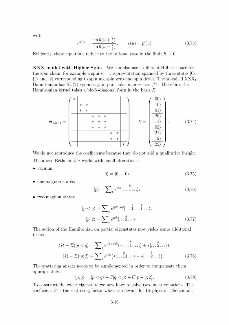
Hamiltonian has SU(2) symmetry, in particular it preserves J z. Therefore, theHamiltonian kernel takes a block-diagonal form in the basis E

Hk,k+1 =

∗∗ ∗∗ ∗

∗ ∗ ∗∗ ∗ ∗∗ ∗ ∗

∗ ∗∗ ∗

∗

, E =

|00〉|10〉|01〉|20〉|11〉|02〉|21〉|12〉|22〉

. (3.74)

We do not reproduce the coefficients because they do not add a qualitative insight.

The above Bethe ansatz works with small alterations:

• vacuum:|0〉 = |0 . . . 0〉. (3.75)

• one-magnon states:

|p〉 =∑

keipk|. . .

k

1 . . .〉. (3.76)

• two-magnon states:

|p < q〉 =∑

keipk+iql|. . .

k

1 . . .l

1 . . .〉,

|p; 2〉 =∑

keipk|. . .

k

2 . . .〉. (3.77)

The action of the Hamiltonian on partial eigenstates now yields some additionalterms

(H− E)|p < q〉 =∑

kei(p+q)k

(∗|. . .

k

11 . . .〉+ ∗|. . .k

2 . . .〉),

(H− E)|p; 2〉 =∑

keipk(∗|. . .

k

11 . . .〉+ ∗|. . .k

2 . . .〉). (3.78)

The scattering ansatz needs to be supplemented in order to compensate themappropriately.

|p, q〉 = |p < q〉+ S|q < p〉+ C|p+ q; 2〉. (3.79)

To construct the exact eigenstate we now have to solve two linear equations. Thecoefficient S is the scattering factor which is relevant for IR physics. The contact

3.16

term C is important for the solution, but it merely describes the UV physics of theeigenstate.24

The resulting Bethe equations for a closed chain read(uk + i

uk − i

)L=

M∏j=1

j 6=k

uk − uj + i

uk − uj − i, eip =

u+ i

u− i, e(u) = p′(u). (3.80)

Note that the Bethe equations are almost the same up to a different prefactor of ion the l.h.s. of the Bethe equations and likewise in the definition of the magnonmomentum.

The generalisation to arbitrary spin s representations at each site is evident (andcorrect) (

uk + is

uk − is

)L=

M∏j=1

j 6=k

uk − uj + i

uk − uj − i, eip =

u+ is

u− is. (3.81)

The corresponding model is called the XXXs model.

Bethe Ansatz at Higher Rank. Generalisation of the XXX model tohigher-rank groups exist. For example, consider a chain with SU(N) symmetryand spins in the fundamental representation

V = CN , |1〉, . . . , |N〉 ∈ V. (3.82)

An integrable nearest neighbour Hamiltonian is given by the kernel

Hk,k+1 = Ik,k+1 − Pk,k+1. (3.83)

More explicitly, this kernel acts as follows

H|ab〉 = |ab〉 − |ba〉. (3.84)

We can again perform the Bethe ansatz:

• vacuum:|0〉 = |1 . . . 1〉. (3.85)

• there are now N − 1 flavours of one-magnon states labelled by a = 2, . . . N

|p, a〉 =∑

keipk|. . . ka . . .〉. (3.86)

24The term |p+ 2; 2〉 should be viewed as a contribution when both magnons reside on a singlesite. We did not have to consider such terms before because for spin 1/2 a single site can only beexcited once.

3.17

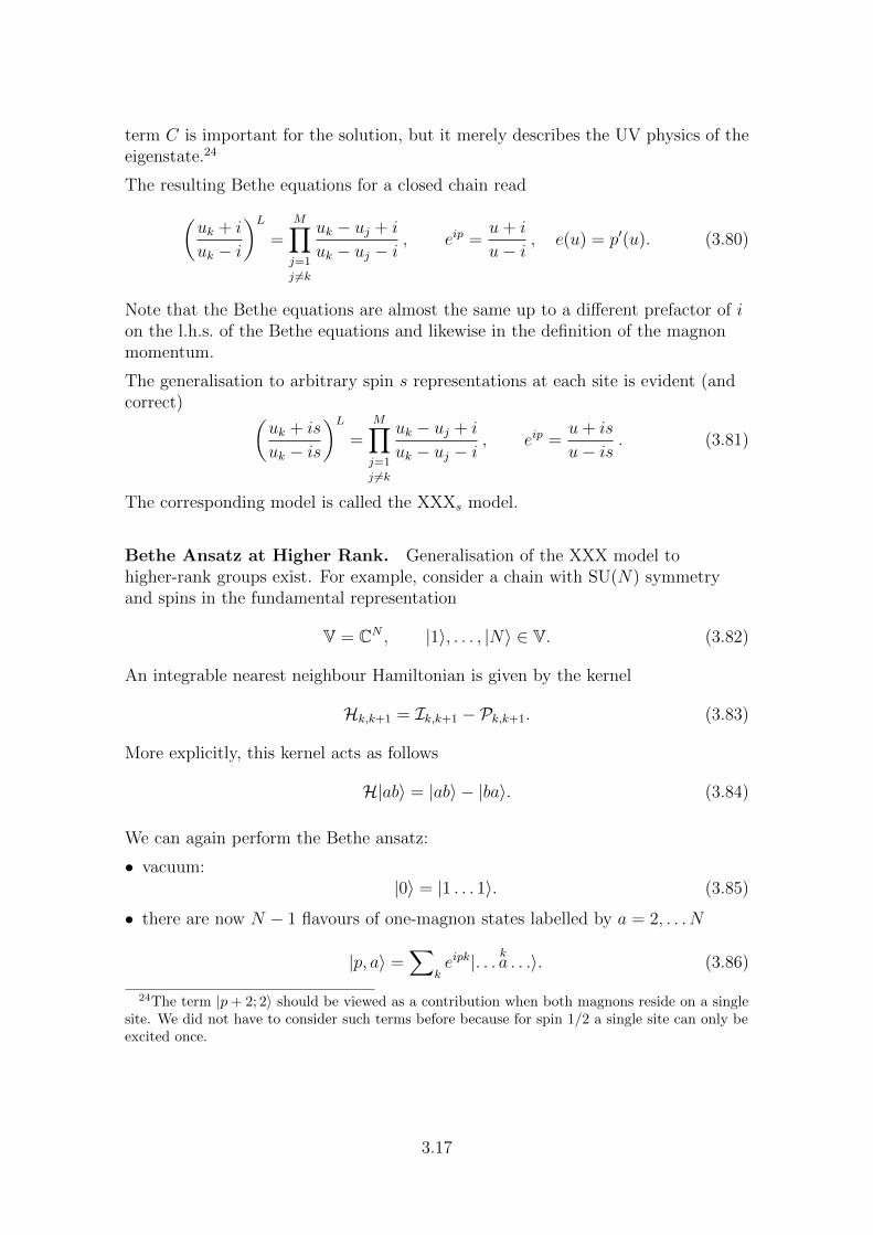
• To accommodate for the various combinations of magnon flavours, we need ascattering matrix 25 instead of a scattering factor for the definition oftwo-magnon states∣∣(p, a), (q, b)

⟩=∣∣(p, a) < (q, b)

⟩+

N∑c,d=2

Scdab(p, q)∣∣(q, d) < (p, c)

⟩. (3.87)

The S-matrix may again be represented graphically as follows:

p, a q, b

p, cq, d

S (3.88)

The scattering matrix is a new feature for models based on a higher-rank algebra.

• The matrix can be computed as before by matching all asymptotic regions. Inour case, one finds

Scdab(u, v) =(u− v)δcaδ

db + iδdaδ

cb

u− v − i. (3.89)

• It preserves the residual SU(N − 1) of the magnons on the vacuum state.• For u→∞ or v →∞ it is trivial

Scdab(∞, v) = Scdab(u,∞) = δcaδdb . (3.90)

• For equal rapidities it reads

Scdab(u, u) = −δdaδcb . (3.91)

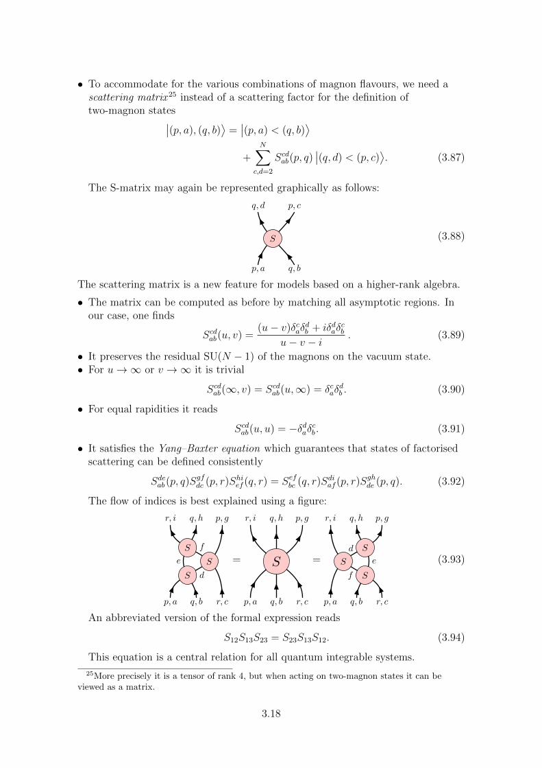
• It satisfies the Yang–Baxter equation which guarantees that states of factorisedscattering can be defined consistently

Sdeab(p, q)Sgfdc (p, r)Shief (q, r) = Sefbc (q, r)Sdiaf (p, r)S

ghde (p, q). (3.92)

The flow of indices is best explained using a figure:

p, a q, b r, c

p, gq, hr, i

e

d

f

S

S

S

=

p, a q, b r, c

p, gq, hr, i

S =

p, a q, b r, c

p, gq, hr, i

e

f

d S

S

S

(3.93)

An abbreviated version of the formal expression reads

S12S13S23 = S23S13S12. (3.94)

This equation is a central relation for all quantum integrable systems.

25More precisely it is a tensor of rank 4, but when acting on two-magnon states it can beviewed as a matrix.

3.18

Nested Bethe Ansatz. The S-matrix now changes the flavour of the particleswhich are scattering. We thus cannot (easily) set up a consistency equation forperiodic wave functions. We would like to “diagonalise” the S-matrix. However,there is no universal method to diagonalise a tensor, but this procedure has to becarefully designed for the problem in question:

• Step 1: Consider a new vacuum state

|0〉2 = |2122 . . . 2M〉 :=∣∣(p1, 2), . . . , (pM , 2)

⟩. (3.95)

The S-matrix is applied easily to this state because scattering is automatically aplain factor S22

22(p, q).• Step 2: Introduce a new types of excitations on the above vacuum

∣∣(u, a)⟩2

=M∑k=1

ψk(u)|21 . . . 2k−1ak2k+1 . . . 2M〉. (3.96)

There are now N − 2 types of excitations labelled by a = 3, . . . , N . The newwave function ψk(u) is not a plane wave because the vacuum state |0〉2 is nothomogeneous. It must be carefully chosen to enable an easy construction ofscattering states and thus it depends on all the underlying magnon momenta pk.We refrain from presenting the details.• Step 3: Constructing states with two new excitations lead to a new S-matrix S2

with (N − 2)4 components. This S-matrix has precisely the same form as theprevious one but with fewer components.

This procedure is reminiscent of the Bethe ansatz. In terms of states andexcitations, we have achieved the following:

spins

|1〉|2〉|3〉...|N〉

=⇒

magnons

|1〉|1〉 → |2〉|1〉 → |3〉

...|1〉 → |N〉

=⇒

excitations

|1〉|1〉 → |2〉|2〉 → |3〉

...|2〉 → |N〉

(3.97)

The Bethe ansatz singles out the vacuum state |1〉 and converts all other spinstates to magnon excitations |1〉 → |a〉 with a = 2, . . . N . The next step singles outone of the magnon excitations |1〉 → |2〉 and declares it as a new vacuum. Theremaining magnons are obtained as new excitations |2〉 → |a〉 of the new vacuumwith a = 3, . . . N . The procedure, called the nested Bethe ansatz can be iteratedN − 1 times in total. At the end we are left with

• the vacuum state |1〉,• the magnon excitation |1〉 → |2〉,• N − 2 higher excitations |a− 1〉 → |a〉 with a = 3, . . . , N .

3.19

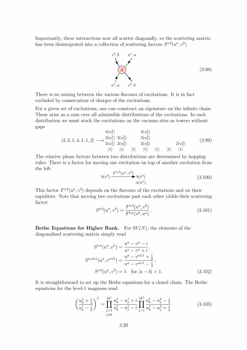
Importantly, these interactions now all scatter diagonally, so the scattering matrixhas been disintegrated into a collection of scattering factors Sa,b(ua, vb)

ua, a vb, b

ua, avb, b

S (3.98)

There is no mixing between the various flavours of excitations. It is in factexcluded by conservation of charges of the excitations.

For a given set of excitations, one can construct an eigenstate on the infinite chain.These arise as a sum over all admissible distributions of the excitations. In eachdistribution we must stack the excitations on the vacuum sites as towers withoutgaps

|4, 3, 1, 4, 1, 1, 2〉 −→

|1〉 |1〉 |1〉 |1〉 |1〉 |1〉 |1〉2(u21) 2(u22) 2(u23) 2(u24)

3(u31) 3(u32) 3(u33)

4(u41) 4(u42)

(3.99)

The relative phase factors between two distributions are determined by hoppingrules: There is a factor for moving one excitation on top of another excitation fromthe left.

a(ua)

b(vb)b(vb)F a,b(ua, vb)

(3.100)

This factor F a,b(ua, vb) depends on the flavours of the excitations and on theirrapidities. Note that moving two excitations past each other yields their scatteringfactor

Sa,b(ua, vb) =F a,b(ua, vb)

F b,a(vb, ua). (3.101)

Bethe Equations for Higher Rank. For SU(N), the elements of thediagonalised scattering matrix simply read

Sa,a(ua, va) =ua − va − iua − va + i

,

Sa,a±1(ua, va±1) =ua − va±1 + i

2

ua − va±1 − i2

,

Sa,b(ua, vb) = 1 for |a− b| > 1. (3.102)

It is straightforward to set up the Bethe equations for a closed chain. The Betheequations for the level-1 magnons read(

u1k + i2

u1k − i2

)L=

M1∏j=1

j 6=k

u1k − u1j + i

u1k − u1j − i

M2∏j=1

u1k − u2j − i2

u1k − u2j + i2

. (3.103)

3.20

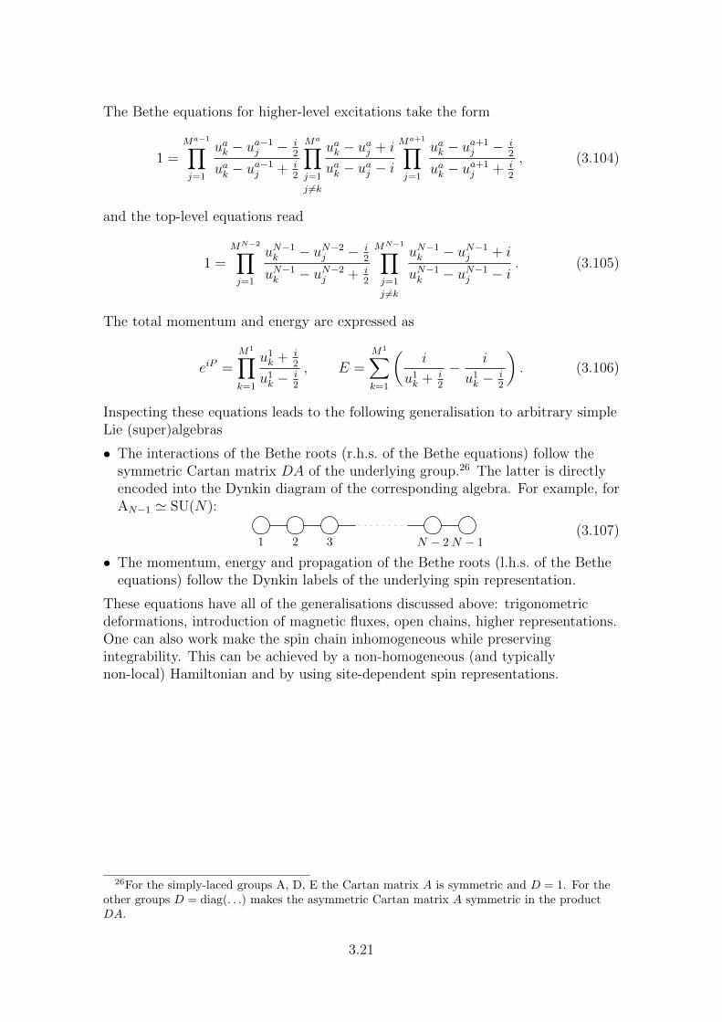
The Bethe equations for higher-level excitations take the form

1 =Ma−1∏j=1

uak − ua−1j − i2

uak − ua−1j + i

2

Ma∏j=1

j 6=k

uak − uaj + i

uak − uaj − i

Ma+1∏j=1

uak − ua+1j − i

2

uak − ua+1j + i

2

, (3.104)

and the top-level equations read

1 =MN−2∏j=1

uN−1k − uN−2j − i2

uN−1k − uN−2j + i2

MN−1∏j=1

j 6=k

uN−1k − uN−1j + i

uN−1k − uN−1j − i. (3.105)

The total momentum and energy are expressed as

eiP =M1∏k=1

u1k + i2

u1k − i2

, E =M1∑k=1

(i

u1k + i2

− i

u1k − i2

). (3.106)

Inspecting these equations leads to the following generalisation to arbitrary simpleLie (super)algebras

• The interactions of the Bethe roots (r.h.s. of the Bethe equations) follow thesymmetric Cartan matrix DA of the underlying group.26 The latter is directlyencoded into the Dynkin diagram of the corresponding algebra. For example, forAN−1 ' SU(N):

1 2 3 N − 2N − 1(3.107)

• The momentum, energy and propagation of the Bethe roots (l.h.s. of the Betheequations) follow the Dynkin labels of the underlying spin representation.

These equations have all of the generalisations discussed above: trigonometricdeformations, introduction of magnetic fluxes, open chains, higher representations.One can also work make the spin chain inhomogeneous while preservingintegrability. This can be achieved by a non-homogeneous (and typicallynon-local) Hamiltonian and by using site-dependent spin representations.

26For the simply-laced groups A, D, E the Cartan matrix A is symmetric and D = 1. For theother groups D = diag(. . .) makes the asymmetric Cartan matrix A symmetric in the productDA.

3.21

Integrability in QFT and AdS/CFT Chapter 4ABGP Doctoral School, 2014 Niklas Beisert

17. 12. 2014

4 Quantum Integrability

Next we would like to discuss a formalism to deal with a large class of quantumintegrable systems.

4.1 R-Matrix Formalism

In the above nested Bethe ansatz we have

• started with an SU(N) fundamental spin chain,• reduced it to magnons with SU(N − 1) residual symmetry,• reduced it further to excitations with SU(N − 2) residual symmetry,• . . .• obtained a final set of excitations with no residual symmetry.

An interesting observation is that in every step we obtained a scattering matrix ofthe same form

Scdab(u, v) =(u− v)δcaδ

db + iδdaδ

cb

u− v − i. (4.1)

In the first step the indices a, b, c, d = 2, . . . , N took N − 1 values, and in the laststep they were all fixed a, b, c, d = N .

Since nothing much changed in each step of the nested Bethe ansatz, we can take astep backwards from the first level and consider the so-called R-matrix

Rcdab(u, v) =

(u− v)δcaδdb + iδdaδ

cb

u− v + i, (4.2)

where a, b, c, d = 1, . . . N . This matrix enjoys the full SU(N) symmetry of the spinchain as well as a couple of features to be discussed below which make it ideallysuited for the construction and investigation of quantum integrable models. Itdiffers from the above scattering matrices by an overall prefactor of(u− v − i)/(u− v + i) which will be largely inconsequential but convenient.

R-Matrix Notations. Before we discuss the properties of R-matrices whichcome to use in the construction of integrable systems we shall introduce somenotation for combining R-matrices which is very helpful for working out identities.

The R-matrix is a linear operator acting on the tensor square of the vector spaceV = CN

R : V⊗ V→ V⊗ V. (4.3)

Moreover, it depends on one complex parameter associated to each of the twovector spaces, R = R(u, v). Here it makes sense to also allow the point at infinityu, v =∞ as a parameter value. In fact, the R-matrix depends only on the

4.1

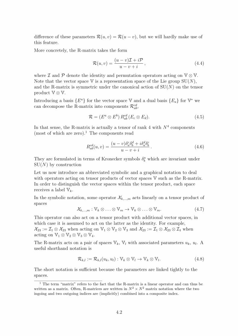
difference of these parameters R(u, v) = R(u− v), but we will hardly make use ofthis feature.

More concretely, the R-matrix takes the form

R(u, v) =(u− v)I + iPu− v + i

, (4.4)

where I and P denote the identity and permutation operators acting on V⊗ V.Note that the vector space V is a representation space of the Lie group SU(N),and the R-matrix is symmetric under the canonical action of SU(N) on the tensorproduct V⊗ V.

Introducing a basis {Ea} for the vector space V and a dual basis {Ea} for V∗ wecan decompose the R-matrix into components Rcd

ab,

R = (Ea ⊗ Eb)Rcdab (Ec ⊗ Ed). (4.5)

In that sense, the R-matrix is actually a tensor of rank 4 with N4 components(most of which are zero).1 The components read

Rcdab(u, v) =

(u− v)δcaδdb + iδdaδ

cb

u− v + i. (4.6)

They are formulated in terms of Kronecker symbols δab which are invariant underSU(N) by construction

Let us now introduce an abbreviated symbolic and a graphical notation to dealwith operators acting on tensor products of vector spaces V such as the R-matrix.In order to distinguish the vector spaces within the tensor product, each spacereceives a label Vk.

In the symbolic notation, some operator Xk,...,m acts linearly on a tensor product ofspaces

Xk,...,m : Vk ⊗ . . .⊗ Vm → Vk ⊗ . . .⊗ Vm. (4.7)

This operator can also act on a tensor product with additional vector spaces, inwhich case it is assumed to act on the latter as the identity. For example,X23 := I1 ⊗X23 when acting on V1 ⊗ V2 ⊗ V3 and X23 := I1 ⊗X23 ⊗ I4 whenacting on V1 ⊗ V2 ⊗ V3 ⊗ V4.

The R-matrix acts on a pair of spaces Vk, Vl with associated parameters uk, ul. Auseful shorthand notation is

Rk,l := Rk,l(uk, ul) : Vk ⊗ Vl → Vk ⊗ Vl. (4.8)

The short notation is sufficient because the parameters are linked tightly to thespaces.

1 The term “matrix” refers to the fact that the R-matrix is a linear operator and can thus bewritten as a matrix. Often, R-matrices are written in N2 ×N2 matrix notation where the twoingoing and two outgoing indices are (implicitly) combined into a composite index.

4.2

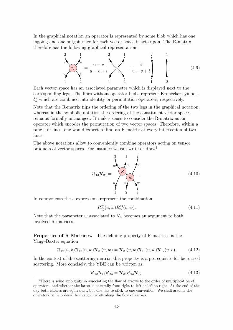
In the graphical notation an operator is represented by some blob which has oneingoing and one outgoing leg for each vector space it acts upon. The R-matrixtherefore has the following graphical representation:

1 2

12

u v

uv

R =u− v

u− v + i

1 2

12

+i

u− v + i

1 2

2 1

. (4.9)

Each vector space has an associated parameter which is displayed next to thecorresponding legs. The lines without operator blobs represent Kronecker symbolsδab which are combined into identity or permutation operators, respectively.

Note that the R-matrix flips the ordering of the two legs in the graphical notation,whereas in the symbolic notation the ordering of the constituent vector spacesremains formally unchanged. It makes sense to consider the R-matrix as anoperator which encodes the permutation of two vector spaces. Therefore, within atangle of lines, one would expect to find an R-matrix at every intersection of twolines.

The above notations allow to conveniently combine operators acting on tensorproducts of vector spaces. For instance we can write or draw2

R13R23 =

1 2 3

1 23

u v w

u vw

RR

. (4.10)

In components these expressions represent the combination

Rdfag(u,w)Reg

bc (v, w). (4.11)

Note that the parameter w associated to V3 becomes an argument to bothinvolved R-matrices.

Properties of R-Matrices. The defining property of R-matrices is theYang–Baxter equation

R12(u, v)R13(u,w)R23(v, w) = R23(v, w)R13(u,w)R12(u, v). (4.12)

In the context of the scattering matrix, this property is a prerequisite for factorisedscattering. More concisely, the YBE can be written as

R12R13R23 = R23R13R12. (4.13)

2There is some ambiguity in associating the flow of arrows to the order of multiplication ofoperators, and whether the latter is naturally from right to left or left to right. At the end of theday both choices are equivalent, but one has to stick to one convention. We shall assume theoperators to be ordered from right to left along the flow of arrows.

4.3

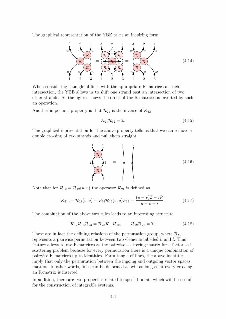
The graphical representation of the YBE takes an inspiring form

1 2 3

123

u v w

uvw

RRR

=

1 2 3

123

R

RR

R

R

=

1 2 3

123

u v w

uvw

RR

R. (4.14)

When considering a tangle of lines with the appropriate R-matrices at eachintersection, the YBE allows us to shift one strand past an intersection of twoother strands. As the figures shows the order of the R-matrices is inverted by suchan operation.

Another important property is that R21 is the inverse of R12

R21R12 = I. (4.15)

The graphical representation for the above property tells us that we can remove adouble crossing of two strands and pull them straight

1 2

12

1 2

R

R

=

1 2

1 2

. (4.16)

Note that for R12 = R12(u, v) the operator R21 is defined as

R21 := R21(v, u) = P12R12(v, u)P12 =(u− v)I − iPu− v − i

. (4.17)

The combination of the above two rules leads to an interesting structure

R12R13R23 = R23R13R12, R12R21 = I . (4.18)

These are in fact the defining relations of the permutation group, where Rk,l

represents a pairwise permutation between two elements labelled k and l. Thisfeature allows to use R-matrices as the pairwise scattering matrix for a factorisedscattering problem because for every permutation there is a unique combination ofpairwise R-matrices up to identities. For a tangle of lines, the above identitiesimply that only the permutation between the ingoing and outgoing vector spacesmatters. In other words, lines can be deformed at will as long as at every crossingan R-matrix is inserted.

In addition, there are two properties related to special points which will be usefulfor the construction of integrable systems.

4.4

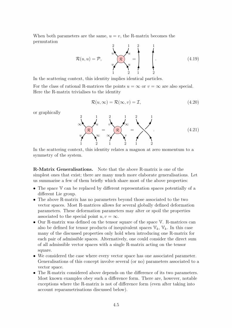
When both parameters are the same, u = v, the R-matrix becomes thepermutation

R(u, u) = P ,

1 2

12

u u

uu

R =

1 2

2 1

. (4.19)

In the scattering context, this identity implies identical particles.

For the class of rational R-matrices the points u =∞ or v =∞ are also special.Here the R-matrix trivialises to the identity

R(u,∞) = R(∞, v) = I, (4.20)

or graphically

1 2

12

u ∞

u∞R =

1 2

12

∞ v

∞v

R =

1 2

12

. (4.21)

In the scattering context, this identity relates a magnon at zero momentum to asymmetry of the system.

R-Matrix Generalisations. Note that the above R-matrix is one of thesimplest ones that exist; there are many much more elaborate generalisations. Letus summarise a few of them briefly which share most of the above properties:

• The space V can be replaced by different representation spaces potentially of adifferent Lie group.• The above R-matrix has no parameters beyond those associated to the two

vector spaces. Most R-matrices allows for several globally defined deformationparameters. These deformation parameters may alter or spoil the propertiesassociated to the special point u, v =∞.• Our R-matrix was defined on the tensor square of the space V. R-matrices can

also be defined for tensor products of inequivalent spaces Vk, Vk. In this casemany of the discussed properties only hold when introducing one R-matrix foreach pair of admissible spaces. Alternatively, one could consider the direct sumof all admissible vector spaces with a single R-matrix acting on the tensorsquare.• We considered the case where every vector space has one associated parameter.

Generalisations of this concept involve several (or no) parameters associated to avector space.• The R-matrix considered above depends on the difference of its two parameters.

Most known examples obey such a difference form. There are, however, notableexceptions where the R-matrix is not of difference form (even after taking intoaccount reparametrisations discussed below).

4.5

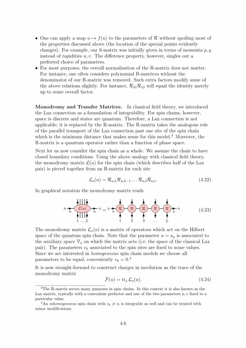
• One can apply a map u 7→ f(u) to the parameters of R without spoiling most ofthe properties discussed above (the location of the special points evidentlychanges). For example, our S-matrix was initially given in terms of momenta p, qinstead of rapidities u, v. The difference property, however, singles out apreferred choice of parameters.• For most purposes, the overall normalisation of the R-matrix does not matter.

For instance, one often considers polynomial R-matrices without thedenominator of our R-matrix was removed. Such extra factors modify some ofthe above relations slightly. For instance, R21R12 will equal the identity merelyup to some overall factor.

Monodromy and Transfer Matrices. In classical field theory, we introducedthe Lax connection as a formulation of integrability. For spin chains, however,space is discrete and states are quantum. Therefore, a Lax connection is notapplicable; it is replaced by the R-matrix. The R-matrix takes the analogous roleof the parallel transport of the Lax connection past one site of the spin chainwhich is the minimum distance that makes sense for this model.3 Moreover, theR-matrix is a quantum operator rather than a function of phase space.

Next let us now consider the spin chain as a whole. We assume the chain to haveclosed boundary conditions. Using the above analogy with classical field theory,the monodromy matrix L(u) for the spin chain (which describes half of the Laxpair) is pieced together from an R-matrix for each site

La(u) = Ra,LRa,L−1 . . .Ra,2Ra,1. (4.22)

In graphical notation the monodromy matrix reads

1 . . . L

a au u

L(u) =

1 2 3 . . . L

a au uR R R R R . (4.23)

The monodromy matrix La(u) is a matrix of operators which act on the Hilbertspace of the quantum spin chain. Note that the parameter u = ua is associated tothe auxiliary space Va on which the matrix acts (i.e. the space of the classical Laxpair). The parameters vk associated to the spin sites are fixed to some values.Since we are interested in homogeneous spin chain models we choose allparameters to be equal, conveniently vk = 0.4

It is now straight-forward to construct charges in involution as the trace of themonodromy matrix

F(u) = tra La(u). (4.24)

3The R-matrix serves many purposes in spin chains. In this context it is also known as theLax matrix, typically with a convenient prefactor and one of the two parameters u, v fixed to aparticular value.

4An inhomogeneous spin chain with vk 6= vl is integrable as well and can be treated withminor modifications.

4.6

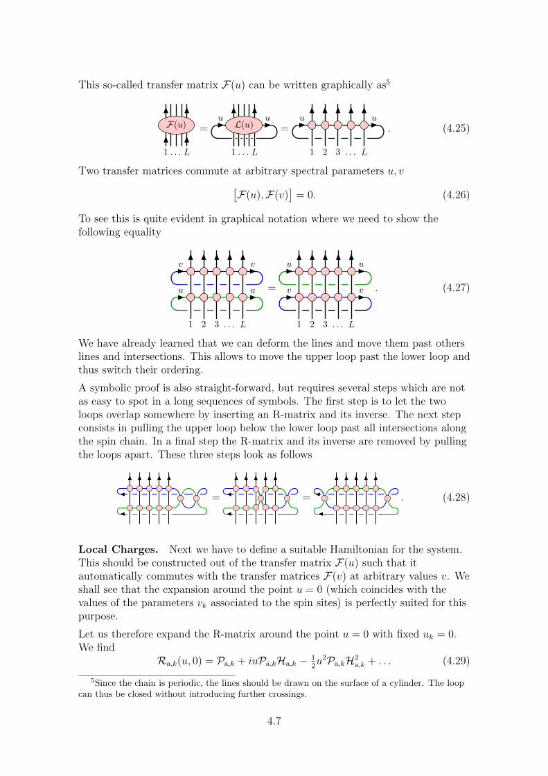
This so-called transfer matrix F(u) can be written graphically as5

1 . . . L

F(u) =

1 . . . L

u uL(u) =

1 2 3 . . . L

u u. (4.25)

Two transfer matrices commute at arbitrary spectral parameters u, v[F(u),F(v)

]= 0. (4.26)

To see this is quite evident in graphical notation where we need to show thefollowing equality

1 2 3 . . . L

u u

v v

=

1 2 3 . . . L

v v

u u

. (4.27)

We have already learned that we can deform the lines and move them past otherslines and intersections. This allows to move the upper loop past the lower loop andthus switch their ordering.

A symbolic proof is also straight-forward, but requires several steps which are notas easy to spot in a long sequences of symbols. The first step is to let the twoloops overlap somewhere by inserting an R-matrix and its inverse. The next stepconsists in pulling the upper loop below the lower loop past all intersections alongthe spin chain. In a final step the R-matrix and its inverse are removed by pullingthe loops apart. These three steps look as follows

= = . (4.28)

Local Charges. Next we have to define a suitable Hamiltonian for the system.This should be constructed out of the transfer matrix F(u) such that itautomatically commutes with the transfer matrices F(v) at arbitrary values v. Weshall see that the expansion around the point u = 0 (which coincides with thevalues of the parameters vk associated to the spin sites) is perfectly suited for thispurpose.

Let us therefore expand the R-matrix around the point u = 0 with fixed uk = 0.We find

Ra,k(u, 0) = Pa,k + iuPa,kHa,k − 12u2Pa,kH2

a,k + . . . (4.29)

5Since the chain is periodic, the lines should be drawn on the surface of a cylinder. The loopcan thus be closed without introducing further crossings.

4.7

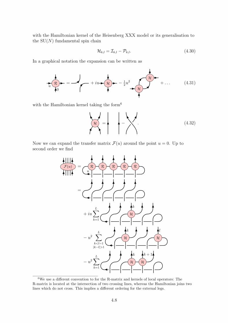
with the Hamiltonian kernel of the Heisenberg XXX model or its generalisation tothe SU(N) fundamental spin chain

Hk,l = Ik,l − Pk,l. (4.30)

In a graphical notation the expansion can be written as

u0

R = + iu H − 12u2

H

H+ . . . (4.31)

with the Hamiltonian kernel taking the form6

H = − . (4.32)

Now we can expand the transfer matrix F(u) around the point u = 0. Up tosecond order we find

F(u) =uR R R R R

=

+ iu

L∑k=1

H

k

− u2L∑

k<l=1|k−l|>1

H

k

H

l

− u2L∑k=1

H

k

H

k + 1

6We use a different convention to for the R-matrix and kernels of local operators: TheR-matrix is located at the intersection of two crossing lines, whereas the Hamiltonian joins twolines which do not cross. This implies a different ordering for the external legs.

4.8

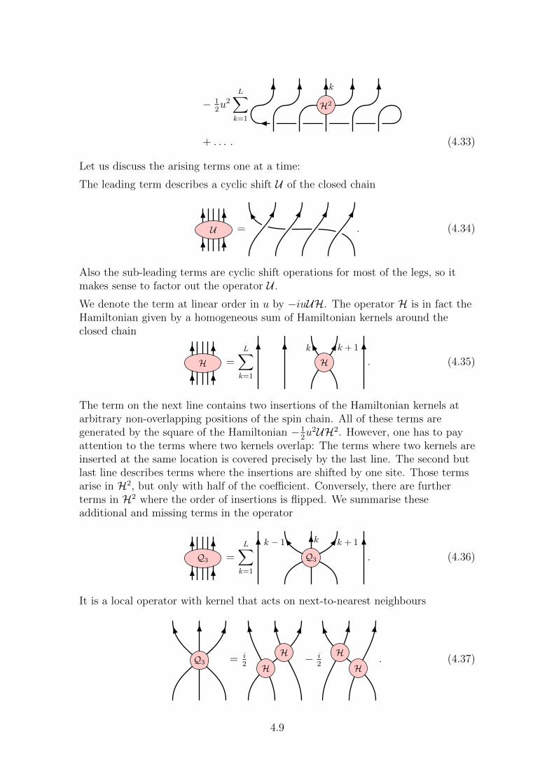
− 12u2

L∑k=1

H2

k

+ . . . . (4.33)

Let us discuss the arising terms one at a time:

The leading term describes a cyclic shift U of the closed chain

U = . (4.34)

Also the sub-leading terms are cyclic shift operations for most of the legs, so itmakes sense to factor out the operator U .

We denote the term at linear order in u by −iuUH. The operator H is in fact theHamiltonian given by a homogeneous sum of Hamiltonian kernels around theclosed chain

H =L∑k=1

k k + 1

H . (4.35)

The term on the next line contains two insertions of the Hamiltonian kernels atarbitrary non-overlapping positions of the spin chain. All of these terms aregenerated by the square of the Hamiltonian −1

2u2UH2. However, one has to pay

attention to the terms where two kernels overlap: The terms where two kernels areinserted at the same location is covered precisely by the last line. The second butlast line describes terms where the insertions are shifted by one site. Those termsarise in H2, but only with half of the coefficient. Conversely, there are furtherterms in H2 where the order of insertions is flipped. We summarise theseadditional and missing terms in the operator

Q3 =L∑k=1

k + 1kk − 1

Q3 . (4.36)

It is a local operator with kernel that acts on next-to-nearest neighbours

Q3 = i2 H

H − i2

H

H. (4.37)

4.9

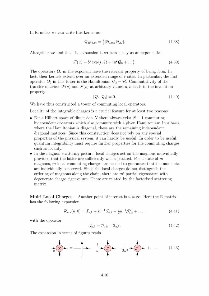
In formulas we can write this kernel as

Q3;k,l,m = i2[Hl,m,Hk,l]. (4.38)

Altogether we find that the expansion is written nicely as an exponential

F(u) = U exp(iuH + iu2Q3 + . . .

). (4.39)

The operators Qr in the exponent have the relevant property of being local. Infact, their kernels extend over an extended range of r sites. In particular, the firstoperator Q2 in this tower is the Hamiltonian Q2 = H. Commutativity of thetransfer matrices F(u) and F(v) at arbitrary values u, v leads to the involutionproperty

[Qr,Qs] = 0. (4.40)

We have thus constructed a tower of commuting local operators.

Locality of the integrable charges is a crucial feature for at least two reasons:

• For a Hilbert space of dimension N there always exist N − 1 commutingindependent operators which also commute with a given Hamiltonian: In a basiswhere the Hamiltonian is diagonal, these are the remaining independentdiagonal matrices. Since this construction does not rely on any specialproperties of the physical system, it can hardly be useful. In order to be useful,quantum integrability must require further properties for the commuting chargessuch as locality.• In the magnon scattering picture, local charges act on the magnons individually

provided that the latter are sufficiently well separated. For a state of mmagnons, m local commuting charges are needed to guarantee that the momentaare individually conserved. Since the local charges do not distinguish theordering of magnons along the chain, there are m! partial eigenstates withdegenerate charge eigenvalues. These are related by the factorised scatteringmatrix.

Multi-Local Charges. Another point of interest is u =∞. Here the R-matrixhas the following expansion

Ra,k(u, 0) = Ia,k + iu−1Ja,k − 12u−2J 2

a,k + . . . , (4.41)

with the operatorJa,k = Pa,k − Ia,k. (4.42)

The expansion in terms of figures reads

u0

R = +i

uJ − 1

2u2J 2 + . . . . (4.43)

4.10

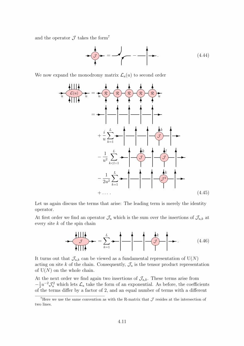
and the operator J takes the form7

J = − . (4.44)

We now expand the monodromy matrix La(u) to second order

u uL(u) = R R R R R

u u

=

+i

u

L∑k=1

Jk

− 1

u2

L∑k<l=1

Jk

Jl

− 1

2u2

L∑k=1

J 2

k

+ . . . . (4.45)

Let us again discuss the terms that arise: The leading term is merely the identityoperator.

At first order we find an operator Ja which is the sum over the insertions of Ja,k atevery site k of the spin chain

J =L∑k=1

Jk

. (4.46)

It turns out that Ja,k can be viewed as a fundamental representation of U(N)acting on site k of the chain. Consequently, Ja is the tensor product representationof U(N) on the whole chain.

At the next order we find again two insertions of Ja,k. These terms arise from−1

2u−2J 2

a which lets La take the form of an exponential. As before, the coefficientsof the terms differ by a factor of 2, and an equal number of terms with a different

7Here we use the same convention as with the R-matrix that J resides at the intersection oftwo lines.

4.11

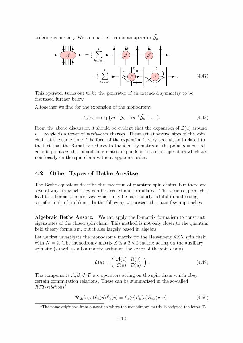
ordering is missing. We summarise them in an operator Ja

J = i2

L∑k<l=1

Jk

Jl

− i2

L∑k<l=1

J

k

J

l

. (4.47)

This operator turns out to be the generator of an extended symmetry to bediscussed further below.

Altogether we find for the expansion of the monodromy

La(u) = exp(iu−1Ja + iu−2Ja + . . .

). (4.48)

From the above discussion it should be evident that the expansion of L(u) aroundu =∞ yields a tower of multi-local charges. These act at several sites of the spinchain at the same time. The form of the expansion is very special, and related tothe fact that the R-matrix reduces to the identity matrix at the point u =∞. Atgeneric points u, the monodromy matrix expands into a set of operators which actnon-locally on the spin chain without apparent order.

4.2 Other Types of Bethe Ansatze

The Bethe equations describe the spectrum of quantum spin chains, but there areseveral ways in which they can be derived and formulated. The various approacheslead to different perspectives, which may be particularly helpful in addressingspecific kinds of problems. In the following we present the main few approaches.

Algebraic Bethe Ansatz. We can apply the R-matrix formalism to constructeigenstates of the closed spin chain. This method is not only closer to the quantumfield theory formalism, but it also largely based in algebra.

Let us first investigate the monodromy matrix for the Heisenberg XXX spin chainwith N = 2. The monodromy matrix L is a 2× 2 matrix acting on the auxiliaryspin site (as well as a big matrix acting on the space of the spin chain)

L(u) =

(A(u) B(u)C(u) D(u)

). (4.49)

The components A,B, C,D are operators acting on the spin chain which obeycertain commutation relations. These can be summarised in the so-calledRTT-relations8

Rab(u, v)La(u)Lb(v) = La(v)Lb(u)Rab(u, v). (4.50)

8The name originates from a notation where the monodromy matrix is assigned the letter T.

4.12

In the graphical notation they read

a

ab

bu

uv

vL(u)

L(v)

R =a

ab

bu

uv

v

L(u)

L(v)

R . (4.51)

They follow straight-forwardly from repeated application of the Yang–Baxterequations.9

We know that our R-matrix is invariant under SU(2), in particular, it preserves thenumber of up and down spins. Consequently, a spin flip in the auxiliary spacemust be compensated by an opposite spin flip on the spin chain. The componentsA and D do not change the number of up and down spins, whereas B and Cincrease and decrease the number of up spins by one unit, respectively.

Recalling that we treated a spin flip as a magnon particle, the above discussion isreminiscent of the framework of quantum field theory where B and C take the rolesof creation and annihilation operators, respectively, whereas A and D serve ascharges. The RTT relations provide the commutation relations which are of thesame kind as the commutation relations for (free) particles, but somewhat moreinvolved.

To construct eigenstates we start again with a ferromagnetic vacuum state

|0〉 = |↓↓ . . . ↓〉. (4.52)

This state is evidently annihilated by C(u) for any u. Excited states are generatedby acting with several B(u)’s on the vacuum.

|u1, . . . , uM〉 = B(u1) . . .B(uM)|0〉. (4.53)

This state has M up spins, and therefore it is an M -magnon state. The ukcorrespond to the magnon rapidities which are related to the magnons by therelation uk = 1

2cot(1

2pk) we used earlier to introduce the rapidity variables. The

operator B(uk) places a magnon with momentum pk on top of the existing magnon.This is done precisely in accordance with the rules to assemble multi-magnon statesdescribed above. All of this construction is neatly encoded into the R-matrix.

So far we have not specified boundary conditions because the monodromy matrixsimply end at the first and the last sites. For a closed chain the latter should berelated as any other pair of adjacent sites. This is achieved by the trace within thetransfer matrix F(u). We are thus interested in its eigenvalues which includes theenergy spectrum of the closed chain. Let us therefore act with

F(u) = A(u) +D(u) (4.54)

9The RTT-relations imply that the monodromy matrix L(u) is an R-matrix as well. ThisR-matrix is slightly more general than the one we discussed above: It acts on two inequivalentspaces, the auxiliary spin site and the Hilbert space of the spin chain. The spin chain spacesupplies not just one parameter v, but rather one parameter vk for each spin site. We merelydecided to set all these parameters to zero vk = 0.

4.13

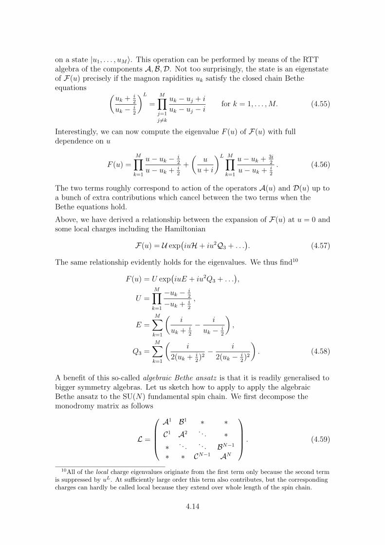
on a state |u1, . . . , uM〉. This operation can be performed by means of the RTTalgebra of the components A,B,D. Not too surprisingly, the state is an eigenstateof F(u) precisely if the magnon rapidities uk satisfy the closed chain Betheequations (

uk + i2

uk − i2

)L=

M∏j=1

j 6=k

uk − uj + i

uk − uj − ifor k = 1, . . . ,M. (4.55)

Interestingly, we can now compute the eigenvalue F (u) of F(u) with fulldependence on u

F (u) =M∏k=1

u− uk − i2

u− uk + i2

+

(u

u+ i

)L M∏k=1

u− uk + 3i2

u− uk + i2

. (4.56)

The two terms roughly correspond to action of the operators A(u) and D(u) up toa bunch of extra contributions which cancel between the two terms when theBethe equations hold.

Above, we have derived a relationship between the expansion of F(u) at u = 0 andsome local charges including the Hamiltonian

F(u) = U exp(iuH + iu2Q3 + . . .

). (4.57)

The same relationship evidently holds for the eigenvalues. We thus find10

F (u) = U exp(iuE + iu2Q3 + . . .

),

U =M∏k=1

−uk − i2

−uk + i2

,

E =M∑k=1

(i

uk + i2

− i

uk − i2

),

Q3 =M∑k=1

(i

2(uk + i2)2− i

2(uk − i2)2

). (4.58)

A benefit of this so-called algebraic Bethe ansatz is that it is readily generalised tobigger symmetry algebras. Let us sketch how to apply to apply the algebraicBethe ansatz to the SU(N) fundamental spin chain. We first decompose themonodromy matrix as follows

L =

A1 B1 ∗ ∗C1 A2 . . . ∗∗ . . . . . . BN−1∗ ∗ CN−1 AN

. (4.59)

10All of the local charge eigenvalues originate from the first term only because the second termis suppressed by uL. At sufficiently large order this term also contributes, but the correspondingcharges can hardly be called local because they extend over whole length of the spin chain.

4.14

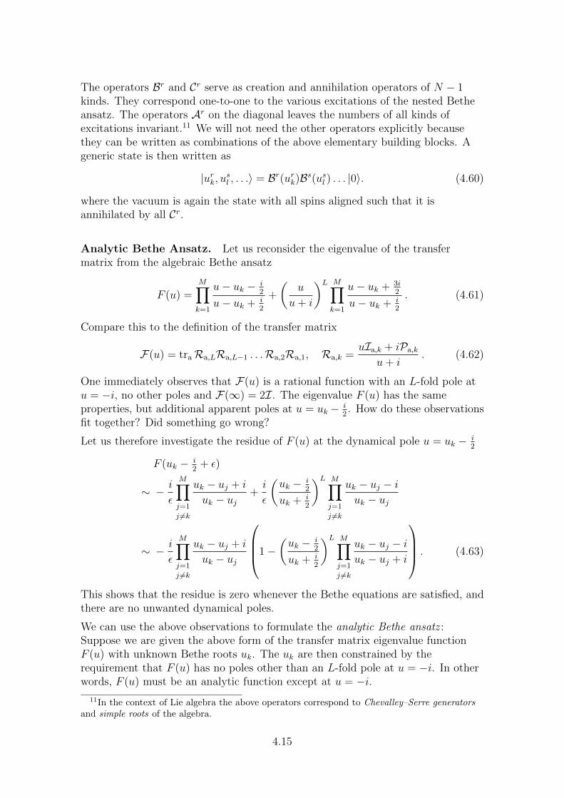
The operators Br and Cr serve as creation and annihilation operators of N − 1kinds. They correspond one-to-one to the various excitations of the nested Betheansatz. The operators Ar on the diagonal leaves the numbers of all kinds ofexcitations invariant.11 We will not need the other operators explicitly becausethey can be written as combinations of the above elementary building blocks. Ageneric state is then written as

|urk, usl , . . .〉 = Br(urk)Bs(usl ) . . . |0〉. (4.60)

where the vacuum is again the state with all spins aligned such that it isannihilated by all Cr.

Analytic Bethe Ansatz. Let us reconsider the eigenvalue of the transfermatrix from the algebraic Bethe ansatz

F (u) =M∏k=1

u− uk − i2

u− uk + i2

+

(u

u+ i

)L M∏k=1

u− uk + 3i2

u− uk + i2

. (4.61)

Compare this to the definition of the transfer matrix

F(u) = traRa,LRa,L−1 . . .Ra,2Ra,1, Ra,k =uIa,k + iPa,k

u+ i. (4.62)

One immediately observes that F(u) is a rational function with an L-fold pole atu = −i, no other poles and F(∞) = 2I. The eigenvalue F (u) has the sameproperties, but additional apparent poles at u = uk − i

2. How do these observations

fit together? Did something go wrong?

Let us therefore investigate the residue of F (u) at the dynamical pole u = uk − i2

F (uk − i2

+ ε)

∼ − i

ε

M∏j=1

j 6=k

uk − uj + i

uk − uj+i

ε

(uk − i

2

uk + i2

)L M∏j=1

j 6=k

uk − uj − iuk − uj

∼ − i

ε

M∏j=1

j 6=k

uk − uj + i

uk − uj

1−(uk − i

2

uk + i2

)L M∏j=1

j 6=k

uk − uj − iuk − uj + i

. (4.63)

This shows that the residue is zero whenever the Bethe equations are satisfied, andthere are no unwanted dynamical poles.

We can use the above observations to formulate the analytic Bethe ansatz :Suppose we are given the above form of the transfer matrix eigenvalue functionF (u) with unknown Bethe roots uk. The uk are then constrained by therequirement that F (u) has no poles other than an L-fold pole at u = −i. In otherwords, F (u) must be an analytic function except at u = −i.

11In the context of Lie algebra the above operators correspond to Chevalley–Serre generatorsand simple roots of the algebra.

4.15

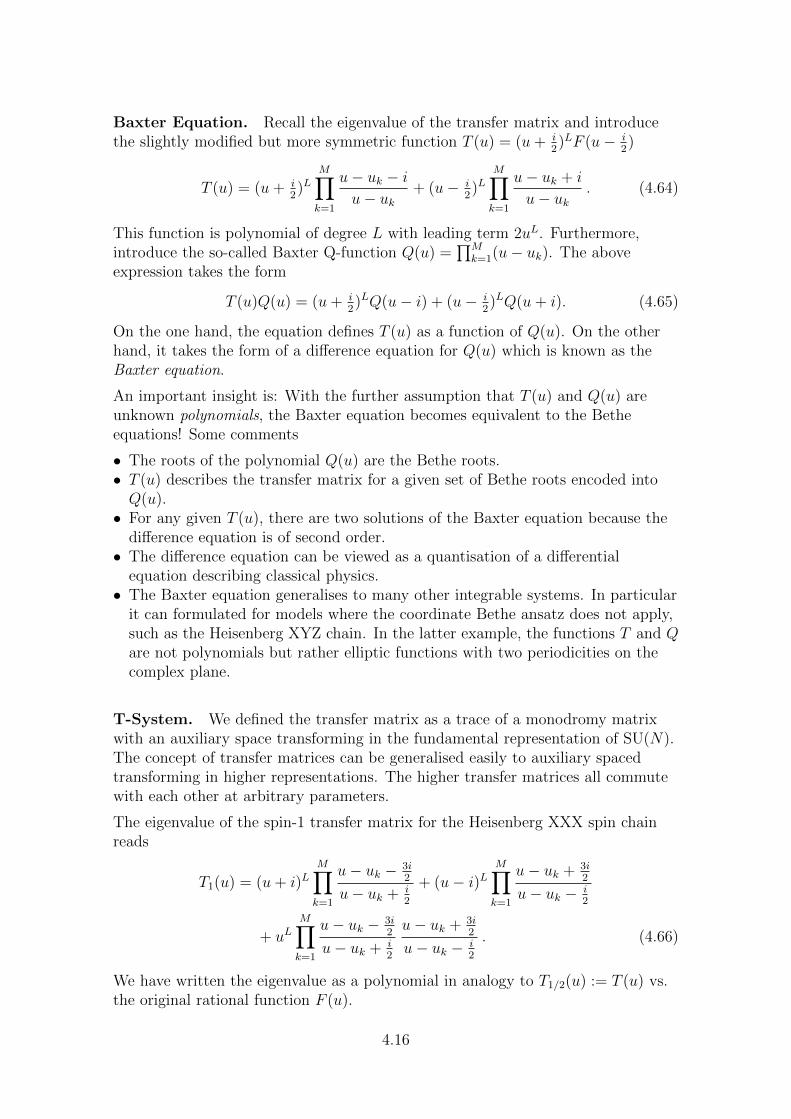
Baxter Equation. Recall the eigenvalue of the transfer matrix and introducethe slightly modified but more symmetric function T (u) = (u+ i

2)LF (u− i

2)

T (u) = (u+ i2)L

M∏k=1

u− uk − iu− uk

+ (u− i2)L

M∏k=1

u− uk + i

u− uk. (4.64)

This function is polynomial of degree L with leading term 2uL. Furthermore,introduce the so-called Baxter Q-function Q(u) =

∏Mk=1(u− uk). The above

expression takes the form

T (u)Q(u) = (u+ i2)LQ(u− i) + (u− i

2)LQ(u+ i). (4.65)

On the one hand, the equation defines T (u) as a function of Q(u). On the otherhand, it takes the form of a difference equation for Q(u) which is known as theBaxter equation.

An important insight is: With the further assumption that T (u) and Q(u) areunknown polynomials, the Baxter equation becomes equivalent to the Betheequations! Some comments

• The roots of the polynomial Q(u) are the Bethe roots.• T (u) describes the transfer matrix for a given set of Bethe roots encoded intoQ(u).• For any given T (u), there are two solutions of the Baxter equation because the

difference equation is of second order.• The difference equation can be viewed as a quantisation of a differential

equation describing classical physics.• The Baxter equation generalises to many other integrable systems. In particular

it can formulated for models where the coordinate Bethe ansatz does not apply,such as the Heisenberg XYZ chain. In the latter example, the functions T and Qare not polynomials but rather elliptic functions with two periodicities on thecomplex plane.

T-System. We defined the transfer matrix as a trace of a monodromy matrixwith an auxiliary space transforming in the fundamental representation of SU(N).The concept of transfer matrices can be generalised easily to auxiliary spacedtransforming in higher representations. The higher transfer matrices all commutewith each other at arbitrary parameters.

The eigenvalue of the spin-1 transfer matrix for the Heisenberg XXX spin chainreads

T1(u) = (u+ i)LM∏k=1

u− uk − 3i2

u− uk + i2

+ (u− i)LM∏k=1

u− uk + 3i2

u− uk − i2

+ uLM∏k=1

u− uk − 3i2

u− uk + i2

u− uk + 3i2

u− uk − i2

. (4.66)

We have written the eigenvalue as a polynomial in analogy to T1/2(u) := T (u) vs.the original rational function F (u).

4.16

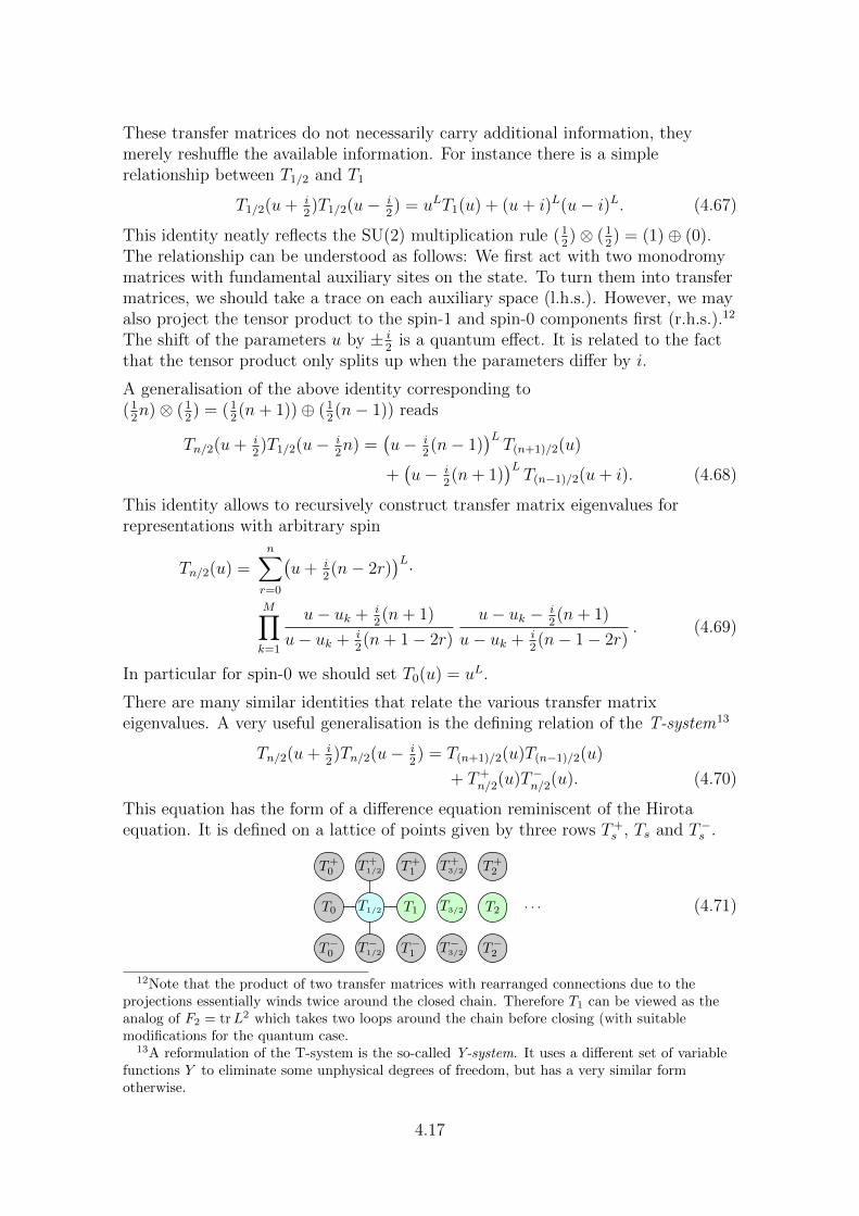
These transfer matrices do not necessarily carry additional information, theymerely reshuffle the available information. For instance there is a simplerelationship between T1/2 and T1

T1/2(u+ i2)T1/2(u− i

2) = uLT1(u) + (u+ i)L(u− i)L. (4.67)

This identity neatly reflects the SU(2) multiplication rule (12)⊗ (1

2) = (1)⊕ (0).

The relationship can be understood as follows: We first act with two monodromymatrices with fundamental auxiliary sites on the state. To turn them into transfermatrices, we should take a trace on each auxiliary space (l.h.s.). However, we mayalso project the tensor product to the spin-1 and spin-0 components first (r.h.s.).12

The shift of the parameters u by ± i2

is a quantum effect. It is related to the factthat the tensor product only splits up when the parameters differ by i.

A generalisation of the above identity corresponding to(12n)⊗ (1

2) = (1

2(n+ 1))⊕ (1

2(n− 1)) reads

Tn/2(u+ i2)T1/2(u− i

2n) =

(u− i

2(n− 1)

)LT(n+1)/2(u)

+(u− i

2(n+ 1)

)LT(n−1)/2(u+ i). (4.68)

This identity allows to recursively construct transfer matrix eigenvalues forrepresentations with arbitrary spin

Tn/2(u) =n∑r=0

(u+ i

2(n− 2r)

)L·M∏k=1

u− uk + i2(n+ 1)

u− uk + i2(n+ 1− 2r)

u− uk − i2(n+ 1)

u− uk + i2(n− 1− 2r)

. (4.69)

In particular for spin-0 we should set T0(u) = uL.

There are many similar identities that relate the various transfer matrixeigenvalues. A very useful generalisation is the defining relation of the T-system13

Tn/2(u+ i2)Tn/2(u− i

2) = T(n+1)/2(u)T(n−1)/2(u)

+ T+n/2(u)T−n/2(u). (4.70)

This equation has the form of a difference equation reminiscent of the Hirotaequation. It is defined on a lattice of points given by three rows T+

s , Ts and T−s .

T0 T1/2 T1 T3/2 T2

T+0 T+

1/2 T+1 T+

3/2 T+2

T−0 T−1/2 T−1 T−3/2 T−2

. . . (4.71)

12Note that the product of two transfer matrices with rearranged connections due to theprojections essentially winds twice around the closed chain. Therefore T1 can be viewed as theanalog of F2 = trL2 which takes two loops around the chain before closing (with suitablemodifications for the quantum case.

13A reformulation of the T-system is the so-called Y-system. It uses a different set of variablefunctions Y to eliminate some unphysical degrees of freedom, but has a very similar formotherwise.

4.17

In our case the top and bottom rows as well as the first site of the middle row aregiven by fixed boundary values

T±n/2(u) =(u± i

2(n+ 1)

)L, T0(u) = uL. (4.72)

The middle row contains the dynamical information on the system. Requiring thatall the Ts(u) are polynomials is equivalent to the Bethe equation and determinesthe spectrum of the closed Heisenberg XXX spin chain.

The benefit of the T-system equation is that it generalises to much morecomplicated systems such as integrable quantum field theories and the so-calledthermodynamic Bethe ansatz. To that end one has to set up a suitable lattice offunctions14 and specify appropriate boundary conditions. The drawback of thisapproach is that the T-system consists of infinitely many functions to be solvedsimultaneously.

14The lattice is closely related to the symmetry algebra: The vertical direction corresponds tothe Dynkin diagram; in our case there is just a single row (after removing the boundaries)corresponding to the single node of the Dynkin diagram for SU(2). The horizontal directioncorresponds to a reduced n-fold symmetric product of the fundamental representationcorresponding to one node of the Dynkin diagram; in our case this is the representation with spin(n/2).

4.18

Integrability in QFT and AdS/CFT Chapter 5ABGP Doctoral School, 2014 Niklas Beisert

17. 12. 2014

5 AdS/CFT Integrability

Topics in this chapter:

• CFT, local operators, anomalous dimensions,• SU(2) sector, spin chain picture, Hamiltonian• SL(2) = SU(1, 1) sector, Bethe equations, PSU(2, 2|4) spin chain• higher-loop corrections, long-range interactions, long-range Bethe equations• wrapping terms, Luscher Corrections, very high loop anomalous dimensions,

multiple zeta values• mirror theory, TBA, T/Y-system, NLIE, quantum curve thermodynamic limit• three-point functions, partial scalar products, determinant formulas• scattering amplitudes, null polygonal Wilson loops, worldsheet area, T-duality,

weak-weak duality, dual conformal symmetry, Yangian symmetry, problem ofdivergences

For further details, please refer to reviews on this subject.

5.1